Embed Size (px)
Citation preview

Part 11: Hypothesis Testing - 2 11-1/78
Econometrics I Professor William Greene
Stern School of Business
Department of Economics
Part 11: Hypothesis Testing - 2 11-2/78
Econometrics I
Part 11 – Hypothesis Testing
Part 11: Hypothesis Testing - 2 11-3/78
Classical Hypothesis Testing
We are interested in using the linear regression
to support or cast doubt on the validity of a
theory about the real world counterpart to our
statistical model. The model is used to test
hypotheses about the underlying data
generating process.
Part 11: Hypothesis Testing - 2 11-4/78
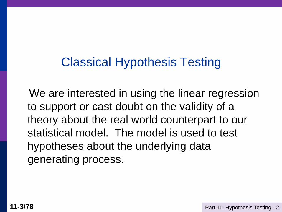
Types of Tests
Nested Models: Restriction on the parameters of a
particular model
y = 1 + 2x + 3T + , 3 = 0
(The “treatment” works; 3 0 .)
Nonnested models: E.g., different RHS variables
yt = 1 + 2xt + 3xt-1 + t
yt = 1 + 2xt + 3yt-1 + wt
(Lagged effects occur immediately or spread over time.)
Specification tests:
~ N[0,2] vs. some other distribution
(The “null” spec. is true or some other spec. is true.)
Part 11: Hypothesis Testing - 2 11-5/78
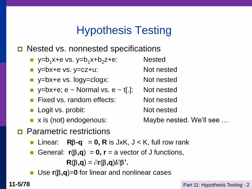
Hypothesis Testing
Nested vs. nonnested specifications
y=b1x+e vs. y=b1x+b2z+e: Nested
y=bx+e vs. y=cz+u: Not nested
y=bx+e vs. logy=clogx: Not nested
y=bx+e; e ~ Normal vs. e ~ t[.]: Not nested
Fixed vs. random effects: Not nested
Logit vs. probit: Not nested
x is (not) endogenous: Maybe nested. We’ll see …
Parametric restrictions
Linear: R-q = 0, R is JxK, J < K, full row rank
General: r(,q) = 0, r = a vector of J functions,
R(,q) = r(,q)/’.
Use r(,q)=0 for linear and nonlinear cases
Part 11: Hypothesis Testing - 2 11-6/78
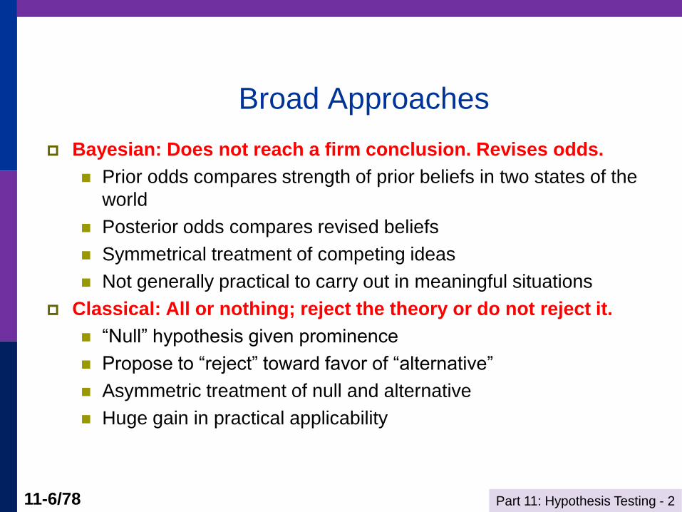
Broad Approaches
Bayesian: Does not reach a firm conclusion. Revises odds.
Prior odds compares strength of prior beliefs in two states of the
world
Posterior odds compares revised beliefs
Symmetrical treatment of competing ideas
Not generally practical to carry out in meaningful situations
Classical: All or nothing; reject the theory or do not reject it.
“Null” hypothesis given prominence
Propose to “reject” toward favor of “alternative”
Asymmetric treatment of null and alternative
Huge gain in practical applicability
Part 11: Hypothesis Testing - 2 11-7/78
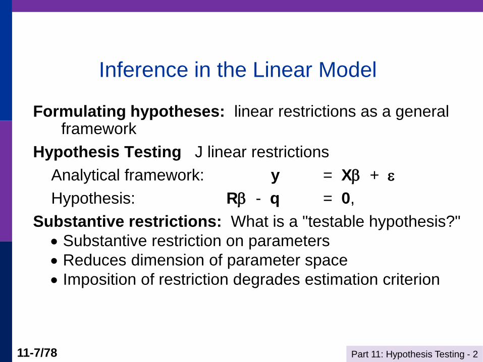
Inference in the Linear Model
Formulating hypotheses: linear restrictions as a general framework
Hypothesis Testing J linear restrictions
Analytical framework: y = X +
Hypothesis: R - q = 0,
Substantive restrictions: What is a "testable hypothesis?"
Substantive restriction on parameters
Reduces dimension of parameter space
Imposition of restriction degrades estimation criterion
Part 11: Hypothesis Testing - 2 11-8/78
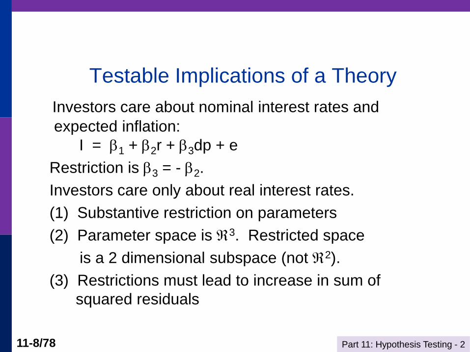
Testable Implications of a Theory
Investors care about nominal interest rates and
expected inflation:
I = 1 + 2r + 3dp + e
Restriction is 3 = - 2.
Investors care only about real interest rates.
(1) Substantive restriction on parameters
(2) Parameter space is 3. Restricted space
is a 2 dimensional subspace (not 2).
(3) Restrictions must lead to increase in sum of
squared residuals
Part 11: Hypothesis Testing - 2 11-9/78
The General Linear Hypothesis: H0: R - q = 0
A unifying departure point: Regardless of the hypothesis, least squares is unbiased.
E[b] =
The hypothesis makes a claim about the population
R – q = 0. Then, if the hypothesis is true, E[Rb – q] = 0.
The sample statistic, Rb – q will not equal zero.
Two possibilities:
Rb – q is small enough to attribute to sampling variability
Rb – q is too large (by some measure) to be plausibly attributed to
sampling variability
Large Rb – q is the rejection region.
Part 11: Hypothesis Testing - 2 11-10/78
Neyman – Pearson Classical Methodology
Formulate null and alternative hypotheses
Hypotheses are exclusive and exhaustive
Null hypothesis is of particular interest
Define “Rejection” region = sample evidence
that will lead to rejection of the null hypothesis.
Gather evidence
Assess whether evidence falls in rejection region
or not.
Part 11: Hypothesis Testing - 2 11-11/78
Testing Fundamentals - I
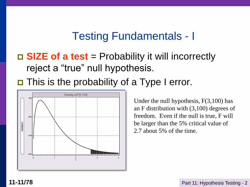
SIZE of a test = Probability it will incorrectly
reject a “true” null hypothesis.
This is the probability of a Type I error.
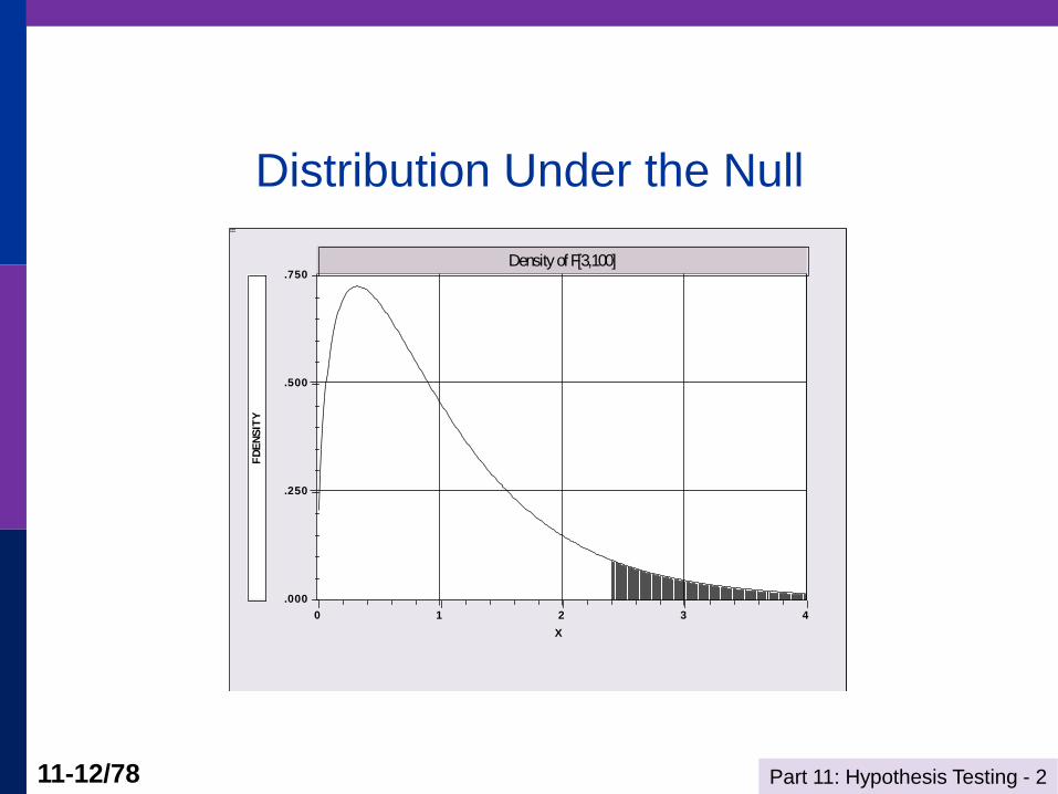
Under the null hypothesis, F(3,100) has
an F distribution with (3,100) degrees of
freedom. Even if the null is true, F will
be larger than the 5% critical value of
2.7 about 5% of the time.
Part 11: Hypothesis Testing - 2 11-12/78
Distribution Under the Null
Density of F[3,100]
X
.250
.500
.750
.000
1 2 3 40
FD
EN
SIT
Y
Part 11: Hypothesis Testing - 2 11-13/78
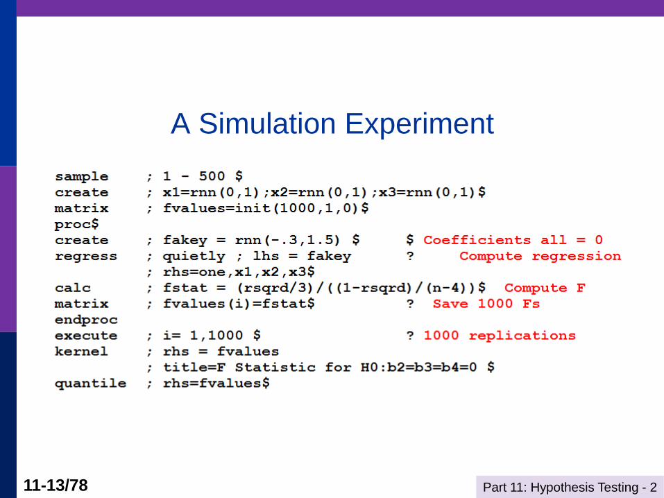
A Simulation Experiment
Part 11: Hypothesis Testing - 2 11-14/78
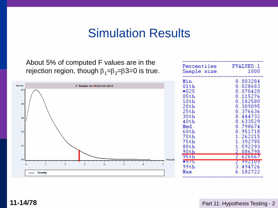
Simulation Results
About 5% of computed F values are in the
rejection region, though 1=2=3=0 is true.
Part 11: Hypothesis Testing - 2 11-15/78
Testing Fundamentals - II
POWER of a test = the probability that it will
correctly reject a “false null” hypothesis
This is 1 – the probability of a Type II error.
The power of a test depends on the specific
alternative.
Part 11: Hypothesis Testing - 2 11-16/78
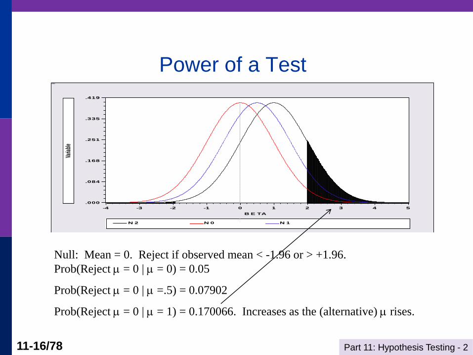
Power of a Test
Null: Mean = 0. Reject if observed mean < -1.96 or > +1.96.
Prob(Reject = 0 | = 0) = 0.05
Prob(Reject = 0 | =.5) = 0.07902
Prob(Reject = 0 | = 1) = 0.170066. Increases as the (alternative) rises.
B E TA
.084
.168
.251
.335
.419
.000
-3 -2 -1 0 1 2 3 4 5-4
N 2 N 0 N 1
Varia
ble
Part 11: Hypothesis Testing - 2 11-17/78
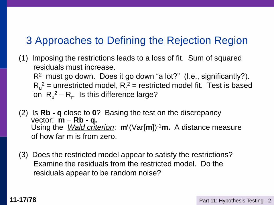
3 Approaches to Defining the Rejection Region
(1) Imposing the restrictions leads to a loss of fit. Sum of squared
residuals must increase.
R2 must go down. Does it go down “a lot?” (I.e., significantly?).
Ru2 = unrestricted model, Rr
2 = restricted model fit. Test is based
on Ru2 – Rr. Is this difference large?
(2) Is Rb - q close to 0? Basing the test on the discrepancy vector: m = Rb - q. Using the Wald criterion: m(Var[m])-1m. A distance measure
of how far m is from zero.
(3) Does the restricted model appear to satisfy the restrictions?
Examine the residuals from the restricted model. Do the
residuals appear to be random noise?
Part 11: Hypothesis Testing - 2 11-18/78
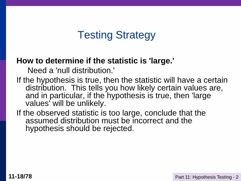
Testing Strategy
How to determine if the statistic is 'large.'
Need a 'null distribution.'
If the hypothesis is true, then the statistic will have a certain distribution. This tells you how likely certain values are, and in particular, if the hypothesis is true, then 'large values' will be unlikely.
If the observed statistic is too large, conclude that the assumed distribution must be incorrect and the hypothesis should be rejected.
Part 11: Hypothesis Testing - 2 11-19/78
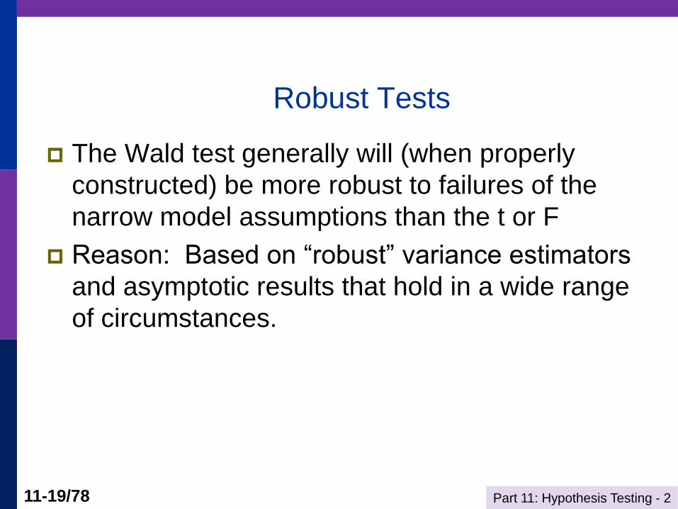
Robust Tests
The Wald test generally will (when properly
constructed) be more robust to failures of the
narrow model assumptions than the t or F
Reason: Based on “robust” variance estimators
and asymptotic results that hold in a wide range
of circumstances.
Part 11: Hypothesis Testing - 2 11-20/78
Part 11: Hypothesis Testing - 2 11-21/78
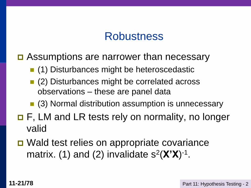
Robustness
Assumptions are narrower than necessary
(1) Disturbances might be heteroscedastic
(2) Disturbances might be correlated across
observations – these are panel data
(3) Normal distribution assumption is unnecessary
F, LM and LR tests rely on normality, no longer
valid
Wald test relies on appropriate covariance
matrix. (1) and (2) invalidate s2(X’X)-1.
Part 11: Hypothesis Testing - 2 11-22/78
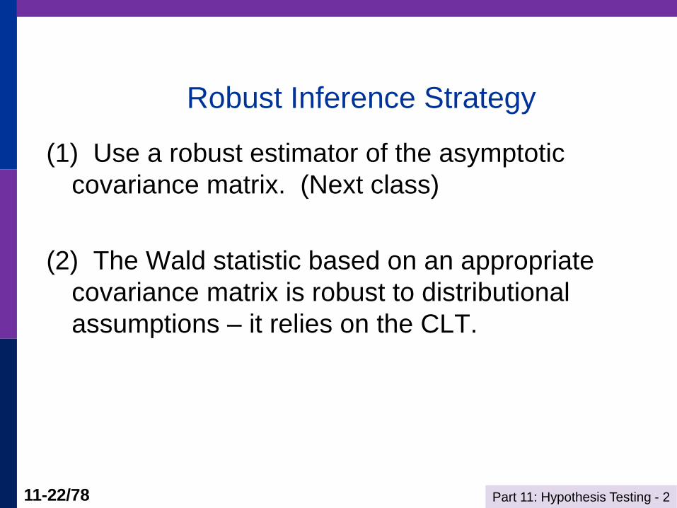
Robust Inference Strategy
(1) Use a robust estimator of the asymptotic
covariance matrix. (Next class)
(2) The Wald statistic based on an appropriate
covariance matrix is robust to distributional
assumptions – it relies on the CLT.
Part 11: Hypothesis Testing - 2 11-23/78
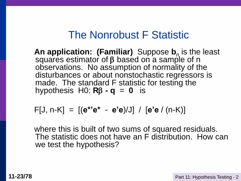
The Nonrobust F Statistic
An application: (Familiar) Suppose bn is the least squares estimator of based on a sample of n observations. No assumption of normality of the disturbances or about nonstochastic regressors is made. The standard F statistic for testing the hypothesis H0: R - q = 0 is
F[J, n-K] = [(e*’e* - e’e)/J] / [e’e / (n-K)]
where this is built of two sums of squared residuals. The statistic does not have an F distribution. How can we test the hypothesis?
Part 11: Hypothesis Testing - 2 11-24/78
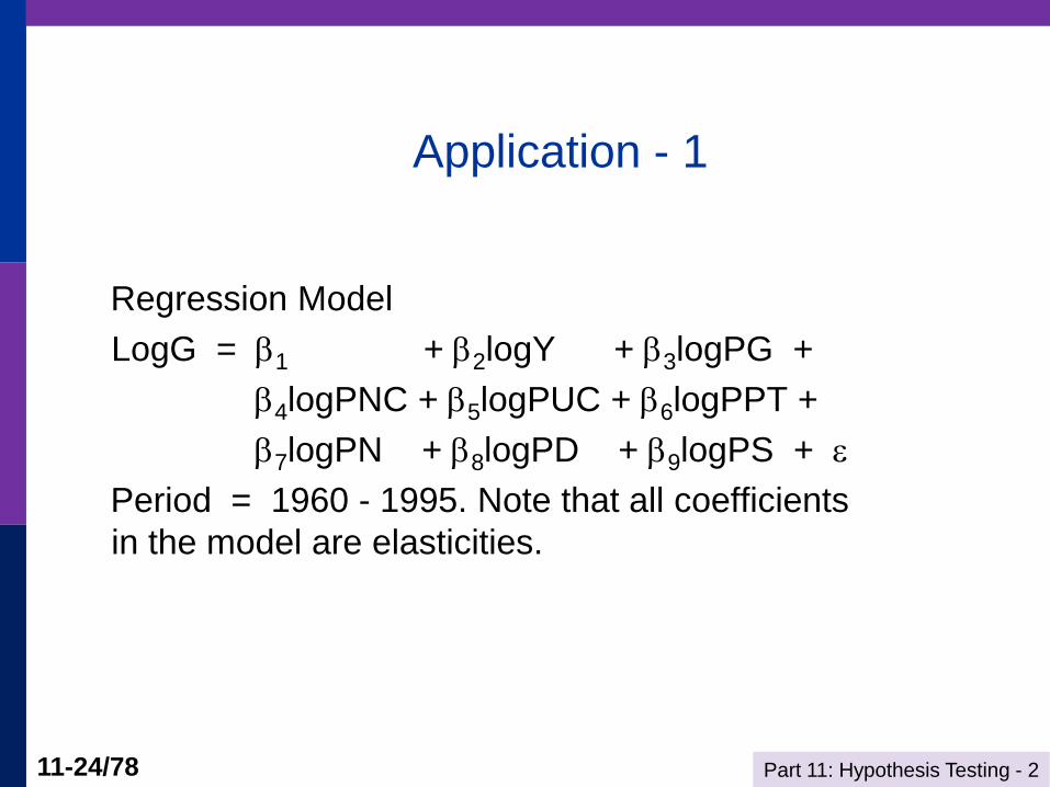
Application - 1
Regression Model
LogG = 1 + 2logY + 3logPG +
4logPNC + 5logPUC + 6logPPT +
7logPN + 8logPD + 9logPS +
Period = 1960 - 1995. Note that all coefficients
in the model are elasticities.
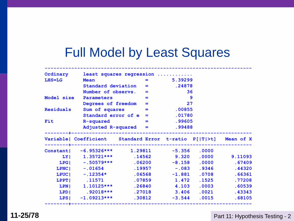
Part 11: Hypothesis Testing - 2 11-25/78
Full Model by Least Squares ----------------------------------------------------------------------
Ordinary least squares regression ............
LHS=LG Mean = 5.39299
Standard deviation = .24878
Number of observs. = 36
Model size Parameters = 9
Degrees of freedom = 27
Residuals Sum of squares = .00855
Standard error of e = .01780
Fit R-squared = .99605
Adjusted R-squared = .99488
--------+-------------------------------------------------------------
Variable| Coefficient Standard Error t-ratio P[|T|>t] Mean of X
--------+-------------------------------------------------------------
Constant| -6.95326*** 1.29811 -5.356 .0000
LY| 1.35721*** .14562 9.320 .0000 9.11093
LPG| -.50579*** .06200 -8.158 .0000 .67409
LPNC| -.01654 .19957 -.083 .9346 .44320
LPUC| -.12354* .06568 -1.881 .0708 .66361
LPPT| .11571 .07859 1.472 .1525 .77208
LPN| 1.10125*** .26840 4.103 .0003 .60539
LPD| .92018*** .27018 3.406 .0021 .43343
LPS| -1.09213*** .30812 -3.544 .0015 .68105
--------+-------------------------------------------------------------
Part 11: Hypothesis Testing - 2 11-26/78
Testing a Hypothesis Using
a Confidence Interval
Given the range of plausible values
Testing the hypothesis that a coefficient equals
zero or some other particular value:
Is the hypothesized value in the confidence
interval?
Is the hypothesized value within the range of
plausible values?
If not, reject the hypothesis.
Part 11: Hypothesis Testing - 2 11-27/78
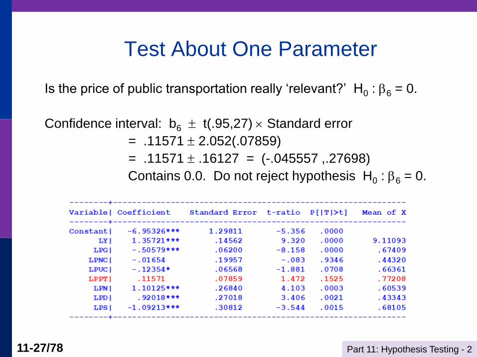
Test About One Parameter
Is the price of public transportation really ‘relevant?’ H0 : 6 = 0.
Confidence interval: b6 t(.95,27) Standard error
= .11571 2.052(.07859)
= .11571 .16127 = (-.045557 ,.27698)
Contains 0.0. Do not reject hypothesis H0 : 6 = 0.
Part 11: Hypothesis Testing - 2 11-28/78
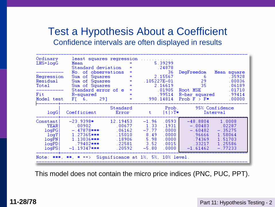
Test a Hypothesis About a Coefficient Confidence intervals are often displayed in results
This model does not contain the micro price indices (PNC, PUC, PPT).
Part 11: Hypothesis Testing - 2 11-29/78
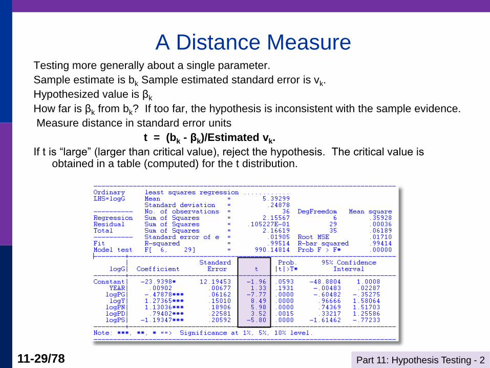
A Distance Measure Testing more generally about a single parameter.
Sample estimate is bk Sample estimated standard error is vk.
Hypothesized value is βk
How far is βk from bk? If too far, the hypothesis is inconsistent with the sample evidence.
Measure distance in standard error units
t = (bk - βk)/Estimated vk.
If t is “large” (larger than critical value), reject the hypothesis. The critical value is obtained in a table (computed) for the t distribution.
Part 11: Hypothesis Testing - 2 11-30/78
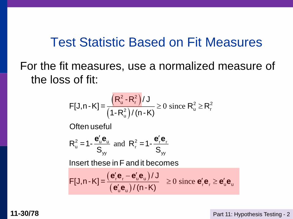
Test Statistic Based on Fit Measures
For the fit measures, use a normalized measure of
the loss of fit:
r rr
r r
r r
0 since
and
0 since
2 2
u r 2 2
u r2
u
2 2u uu
yy yy
u u
u u
u u
R -R / JF[J,n -K] = R R
1-R / (n -K)
Often useful
R =1- R =1-S S
Insert these in F and it becomes
/ JF[J,n -K] =
/ (n -K)
e e e e
e e e ee e e e
e e
Part 11: Hypothesis Testing - 2 11-31/78
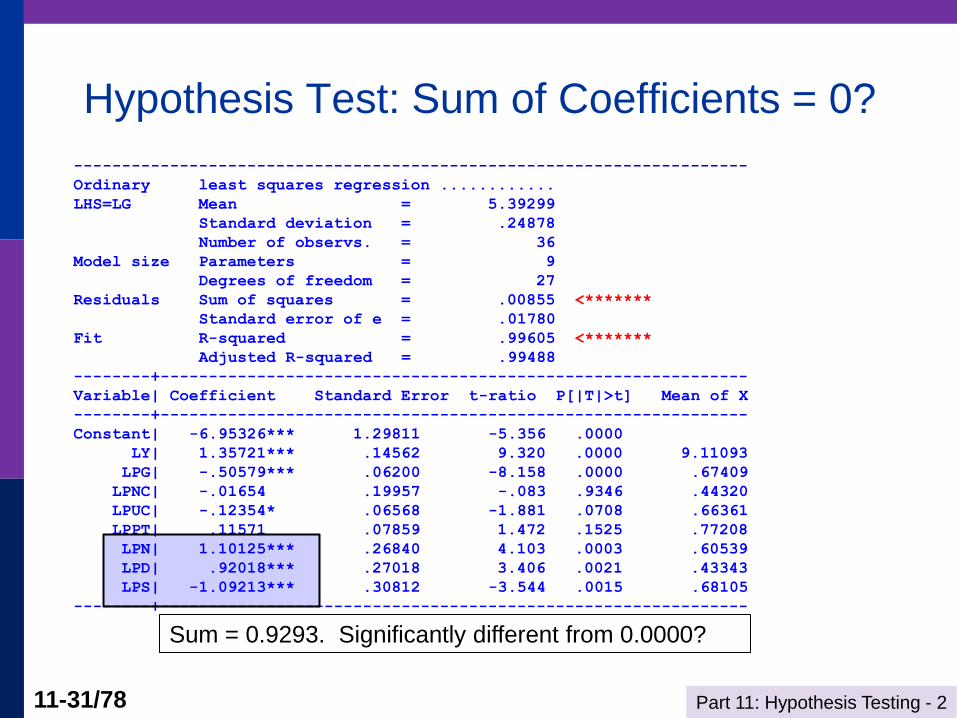
Hypothesis Test: Sum of Coefficients = 0?
----------------------------------------------------------------------
Ordinary least squares regression ............
LHS=LG Mean = 5.39299
Standard deviation = .24878
Number of observs. = 36
Model size Parameters = 9
Degrees of freedom = 27
Residuals Sum of squares = .00855 <*******
Standard error of e = .01780
Fit R-squared = .99605 <*******
Adjusted R-squared = .99488
--------+-------------------------------------------------------------
Variable| Coefficient Standard Error t-ratio P[|T|>t] Mean of X
--------+-------------------------------------------------------------
Constant| -6.95326*** 1.29811 -5.356 .0000
LY| 1.35721*** .14562 9.320 .0000 9.11093
LPG| -.50579*** .06200 -8.158 .0000 .67409
LPNC| -.01654 .19957 -.083 .9346 .44320
LPUC| -.12354* .06568 -1.881 .0708 .66361
LPPT| .11571 .07859 1.472 .1525 .77208
LPN| 1.10125*** .26840 4.103 .0003 .60539
LPD| .92018*** .27018 3.406 .0021 .43343
LPS| -1.09213*** .30812 -3.544 .0015 .68105
--------+-------------------------------------------------------------
Sum = 0.9293. Significantly different from 0.0000?
Part 11: Hypothesis Testing - 2 11-32/78
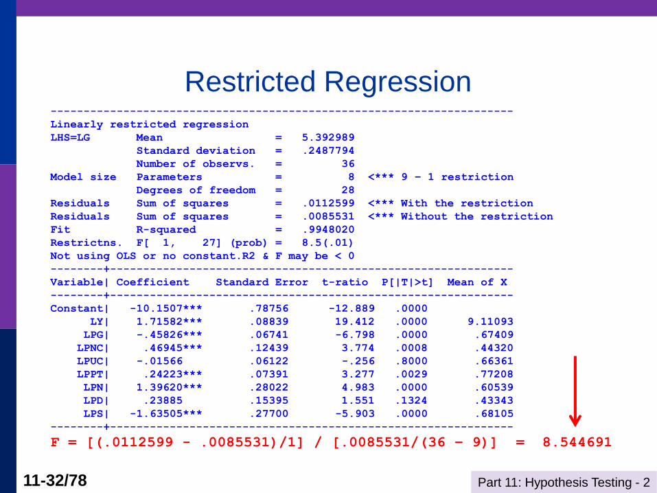
Restricted Regression ----------------------------------------------------------------------
Linearly restricted regression
LHS=LG Mean = 5.392989
Standard deviation = .2487794
Number of observs. = 36
Model size Parameters = 8 <*** 9 – 1 restriction
Degrees of freedom = 28
Residuals Sum of squares = .0112599 <*** With the restriction
Residuals Sum of squares = .0085531 <*** Without the restriction
Fit R-squared = .9948020
Restrictns. F[ 1, 27] (prob) = 8.5(.01)
Not using OLS or no constant.R2 & F may be < 0
--------+-------------------------------------------------------------
Variable| Coefficient Standard Error t-ratio P[|T|>t] Mean of X
--------+-------------------------------------------------------------
Constant| -10.1507*** .78756 -12.889 .0000
LY| 1.71582*** .08839 19.412 .0000 9.11093
LPG| -.45826*** .06741 -6.798 .0000 .67409
LPNC| .46945*** .12439 3.774 .0008 .44320
LPUC| -.01566 .06122 -.256 .8000 .66361
LPPT| .24223*** .07391 3.277 .0029 .77208
LPN| 1.39620*** .28022 4.983 .0000 .60539
LPD| .23885 .15395 1.551 .1324 .43343
LPS| -1.63505*** .27700 -5.903 .0000 .68105
--------+-------------------------------------------------------------
F = [(.0112599 - .0085531)/1] / [.0085531/(36 – 9)] = 8.544691
Part 11: Hypothesis Testing - 2 11-33/78
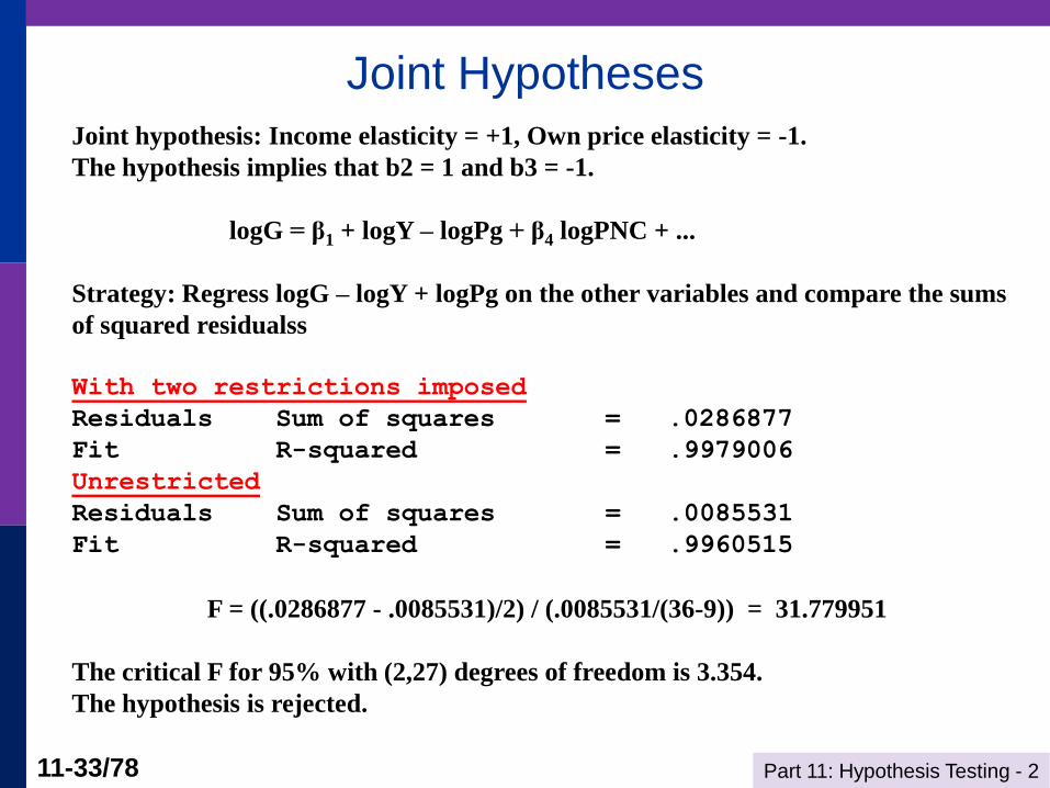
Joint Hypotheses
Joint hypothesis: Income elasticity = +1, Own price elasticity = -1.
The hypothesis implies that b2 = 1 and b3 = -1.
logG = β1 + logY – logPg + β4 logPNC + ...
Strategy: Regress logG – logY + logPg on the other variables and compare the sums
of squared residualss
With two restrictions imposed
Residuals Sum of squares = .0286877
Fit R-squared = .9979006
Unrestricted
Residuals Sum of squares = .0085531
Fit R-squared = .9960515
F = ((.0286877 - .0085531)/2) / (.0085531/(36-9)) = 31.779951
The critical F for 95% with (2,27) degrees of freedom is 3.354.
The hypothesis is rejected.
Part 11: Hypothesis Testing - 2 11-34/78
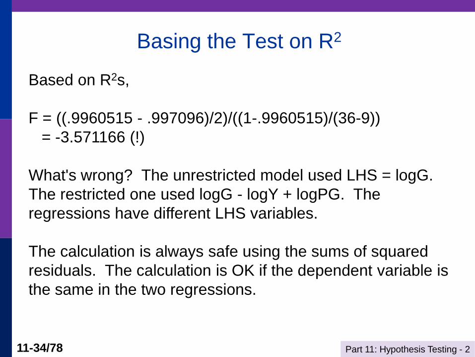
Basing the Test on R2
Based on R2s,
F = ((.9960515 - .997096)/2)/((1-.9960515)/(36-9))
= -3.571166 (!)
What's wrong? The unrestricted model used LHS = logG.
The restricted one used logG - logY + logPG. The
regressions have different LHS variables.
The calculation is always safe using the sums of squared
residuals. The calculation is OK if the dependent variable is
the same in the two regressions.
Part 11: Hypothesis Testing - 2 11-35/78
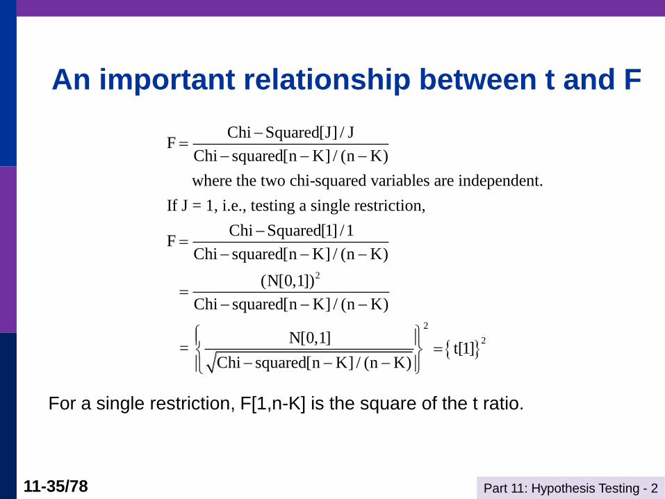
An important relationship between t and F
2
Chi Squared[J] / JF
Chi squared[n K] / (n K)
where the two chi-squared variables are independent.
If J = 1, i.e., testing a single restriction,
Chi Squared[1] /1F
Chi squared[n K] / (n K)
(N[0,1])
Chi s
2
2
quared[n K] / (n K)
N[0,1] = t[1]
Chi squared[n K] / (n K)
For a single restriction, F[1,n-K] is the square of the t ratio.
Part 11: Hypothesis Testing - 2 11-36/78
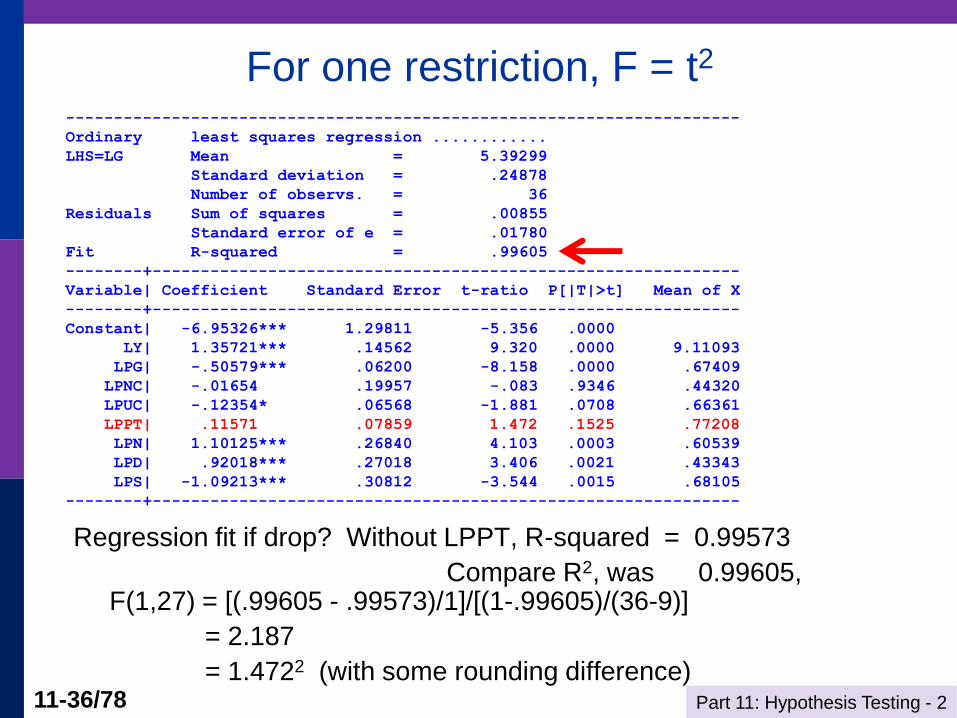
For one restriction, F = t2 ----------------------------------------------------------------------
Ordinary least squares regression ............
LHS=LG Mean = 5.39299
Standard deviation = .24878
Number of observs. = 36
Residuals Sum of squares = .00855
Standard error of e = .01780
Fit R-squared = .99605
--------+-------------------------------------------------------------
Variable| Coefficient Standard Error t-ratio P[|T|>t] Mean of X
--------+-------------------------------------------------------------
Constant| -6.95326*** 1.29811 -5.356 .0000
LY| 1.35721*** .14562 9.320 .0000 9.11093
LPG| -.50579*** .06200 -8.158 .0000 .67409
LPNC| -.01654 .19957 -.083 .9346 .44320
LPUC| -.12354* .06568 -1.881 .0708 .66361
LPPT| .11571 .07859 1.472 .1525 .77208
LPN| 1.10125*** .26840 4.103 .0003 .60539
LPD| .92018*** .27018 3.406 .0021 .43343
LPS| -1.09213*** .30812 -3.544 .0015 .68105
--------+-------------------------------------------------------------
Regression fit if drop? Without LPPT, R-squared = 0.99573
Compare R2, was 0.99605, F(1,27) = [(.99605 - .99573)/1]/[(1-.99605)/(36-9)]
= 2.187
= 1.4722 (with some rounding difference)
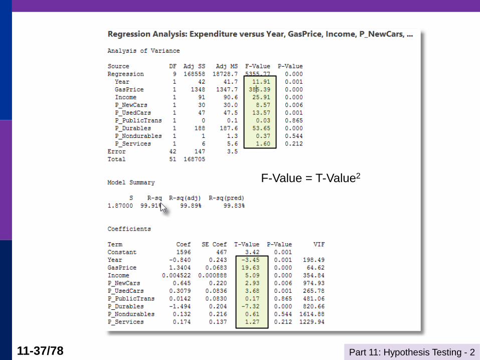
Part 11: Hypothesis Testing - 2 11-37/78
F-Value = T-Value2
Part 11: Hypothesis Testing - 2 11-38/78
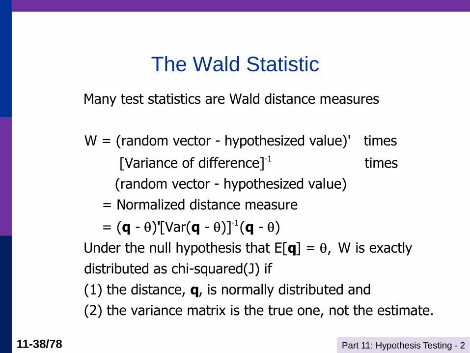
The Wald Statistic
-1
Many test statistics are Wald distance measures
W = (random vector - hypothesized value)' times
[Variance of difference] times
(random vector - hypothesized value)
-1
= Normalized distance measure
= ( - ) [Var( - )] ( - )
Under the null hypothesis that E[ ] = , W is exactly
distributed as chi-squared(J) if
(1) the distance, , is normally distributed a
q ' q q
q
q
nd
(2) the variance matrix is the true one, not the estimate.
Part 11: Hypothesis Testing - 2 11-39/78
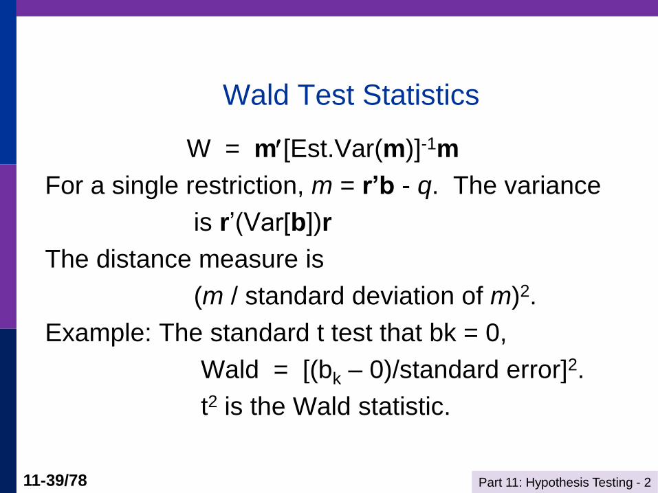
Wald Test Statistics
W = m[Est.Var(m)]-1m
For a single restriction, m = r’b - q. The variance
is r’(Var[b])r
The distance measure is
(m / standard deviation of m)2.
Example: The standard t test that bk = 0,
Wald = [(bk – 0)/standard error]2.
t2 is the Wald statistic.
Part 11: Hypothesis Testing - 2 11-40/78
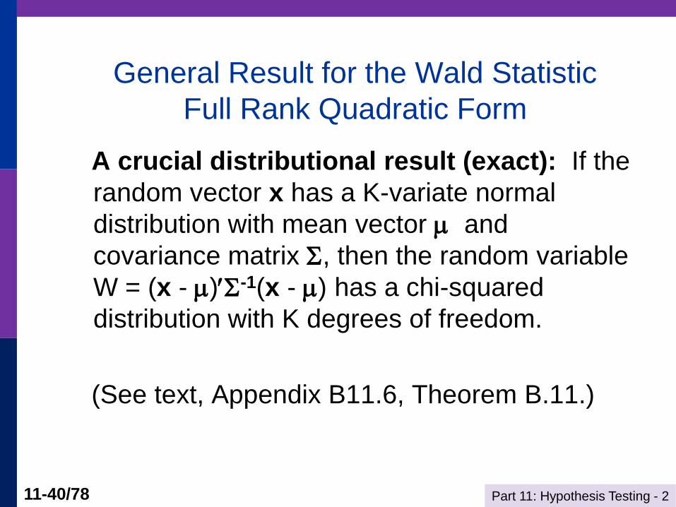
General Result for the Wald Statistic
Full Rank Quadratic Form
A crucial distributional result (exact): If the
random vector x has a K-variate normal
distribution with mean vector and
covariance matrix , then the random variable
W = (x - )-1(x - ) has a chi-squared
distribution with K degrees of freedom.
(See text, Appendix B11.6, Theorem B.11.)
Part 11: Hypothesis Testing - 2 11-41/78
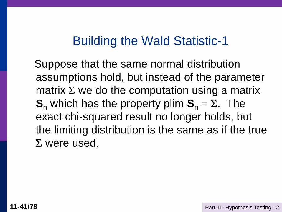
Building the Wald Statistic-1
Suppose that the same normal distribution
assumptions hold, but instead of the parameter
matrix we do the computation using a matrix
Sn which has the property plim Sn = . The
exact chi-squared result no longer holds, but
the limiting distribution is the same as if the true
were used.
Part 11: Hypothesis Testing - 2 11-42/78
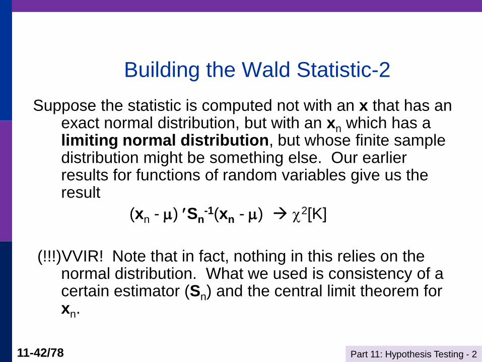
Building the Wald Statistic-2
Suppose the statistic is computed not with an x that has an exact normal distribution, but with an xn which has a limiting normal distribution, but whose finite sample distribution might be something else. Our earlier results for functions of random variables give us the result
(xn - ) Sn-1(xn - ) 2[K]
(!!!)VVIR! Note that in fact, nothing in this relies on the normal distribution. What we used is consistency of a certain estimator (Sn) and the central limit theorem for xn.
Part 11: Hypothesis Testing - 2 11-43/78
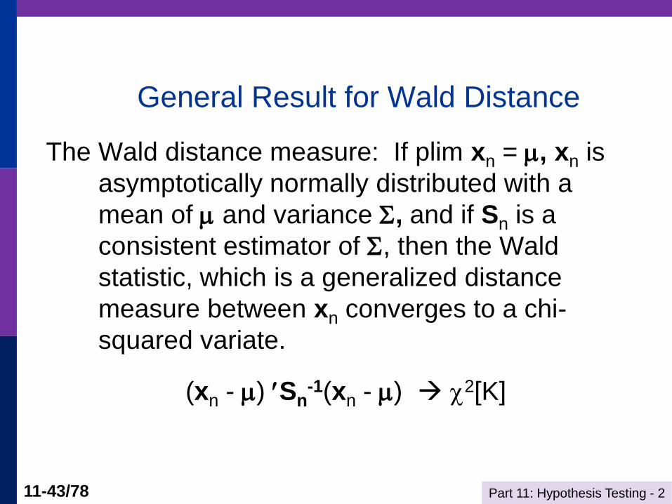
General Result for Wald Distance
The Wald distance measure: If plim xn = , xn is
asymptotically normally distributed with a
mean of and variance , and if Sn is a
consistent estimator of , then the Wald
statistic, which is a generalized distance
measure between xn converges to a chi-
squared variate.
(xn - ) Sn-1(xn - ) 2[K]
Part 11: Hypothesis Testing - 2 11-44/78
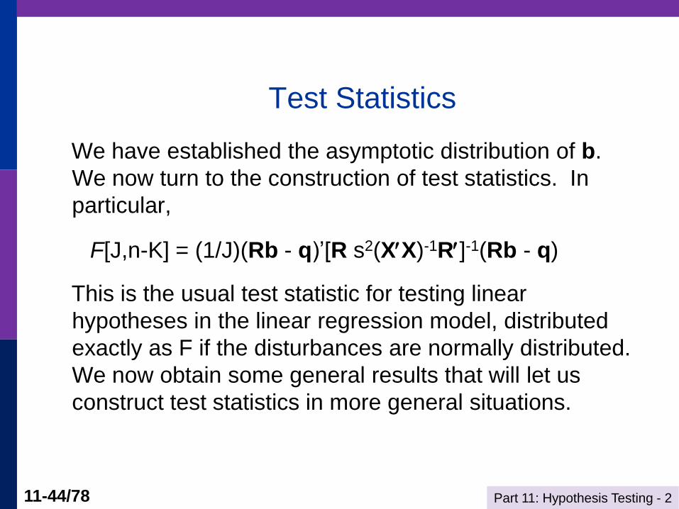
Test Statistics
We have established the asymptotic distribution of b.
We now turn to the construction of test statistics. In
particular,
F[J,n-K] = (1/J)(Rb - q)’[R s2(XX)-1R]-1(Rb - q)
This is the usual test statistic for testing linear
hypotheses in the linear regression model, distributed
exactly as F if the disturbances are normally distributed.
We now obtain some general results that will let us
construct test statistics in more general situations.
Part 11: Hypothesis Testing - 2 11-45/78
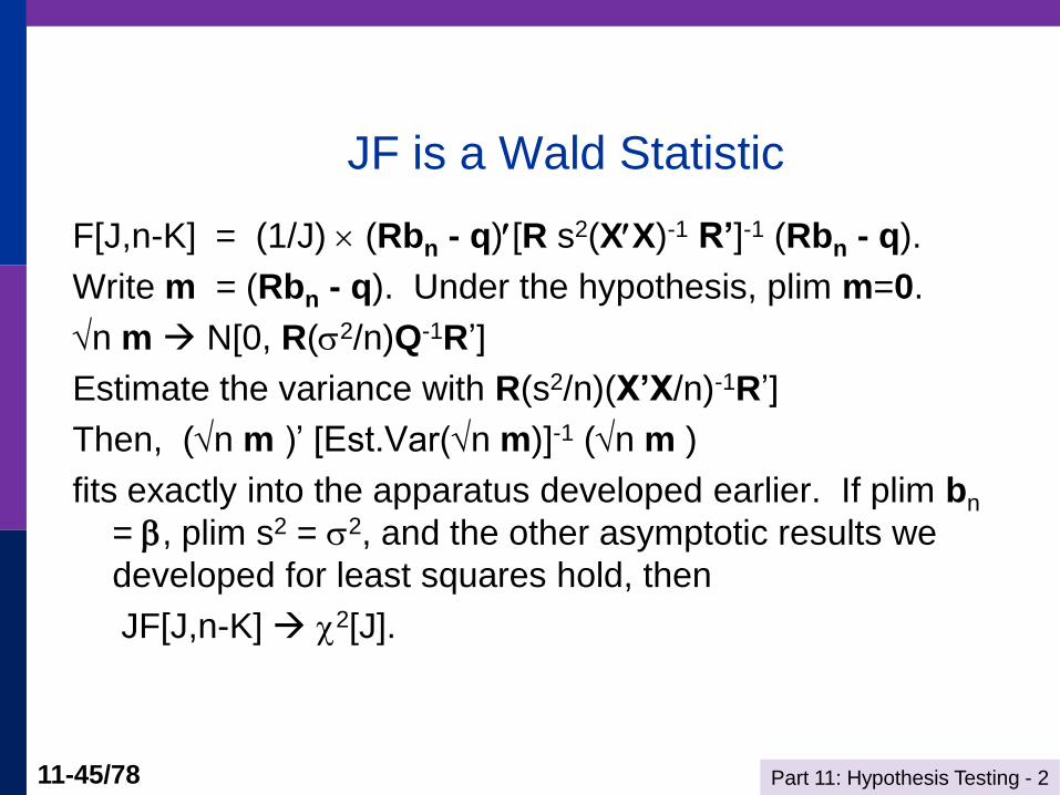
JF is a Wald Statistic
F[J,n-K] = (1/J) (Rbn - q)[R s2(XX)-1 R’]-1 (Rbn - q).
Write m = (Rbn - q). Under the hypothesis, plim m=0.
n m N[0, R(2/n)Q-1R’]
Estimate the variance with R(s2/n)(X’X/n)-1R’]
Then, (n m )’ [Est.Var(n m)]-1 (n m )
fits exactly into the apparatus developed earlier. If plim bn
= , plim s2 = 2, and the other asymptotic results we
developed for least squares hold, then
JF[J,n-K] 2[J].
Part 11: Hypothesis Testing - 2 11-46/78
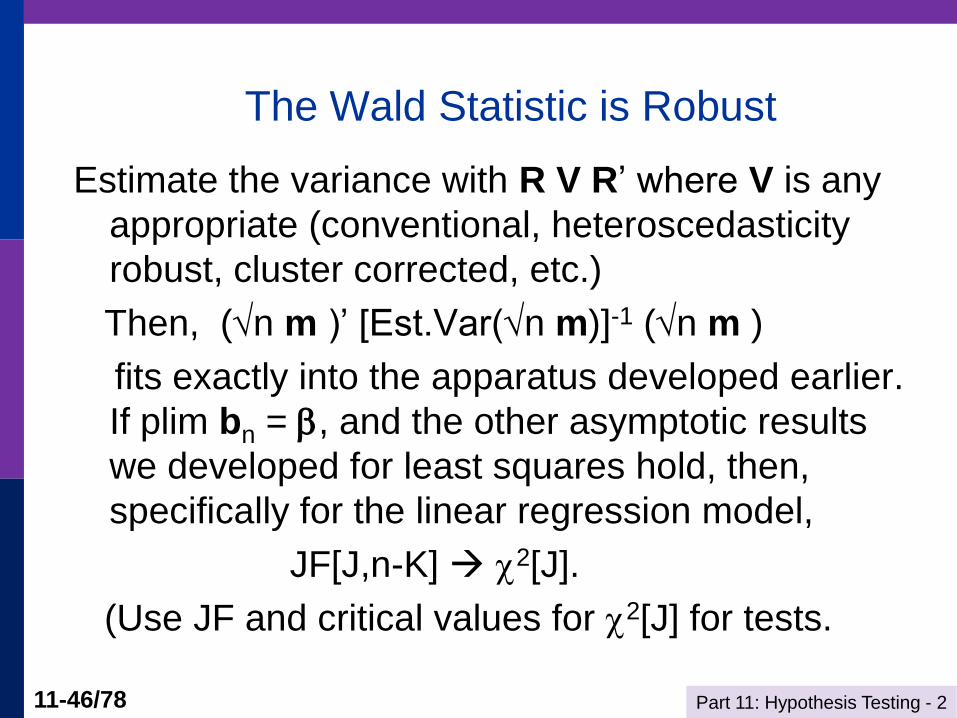
The Wald Statistic is Robust
Estimate the variance with R V R’ where V is any
appropriate (conventional, heteroscedasticity
robust, cluster corrected, etc.)
Then, (n m )’ [Est.Var(n m)]-1 (n m )
fits exactly into the apparatus developed earlier.
If plim bn = , and the other asymptotic results
we developed for least squares hold, then,
specifically for the linear regression model,
JF[J,n-K] 2[J].
(Use JF and critical values for 2[J] for tests.
Part 11: Hypothesis Testing - 2 11-47/78
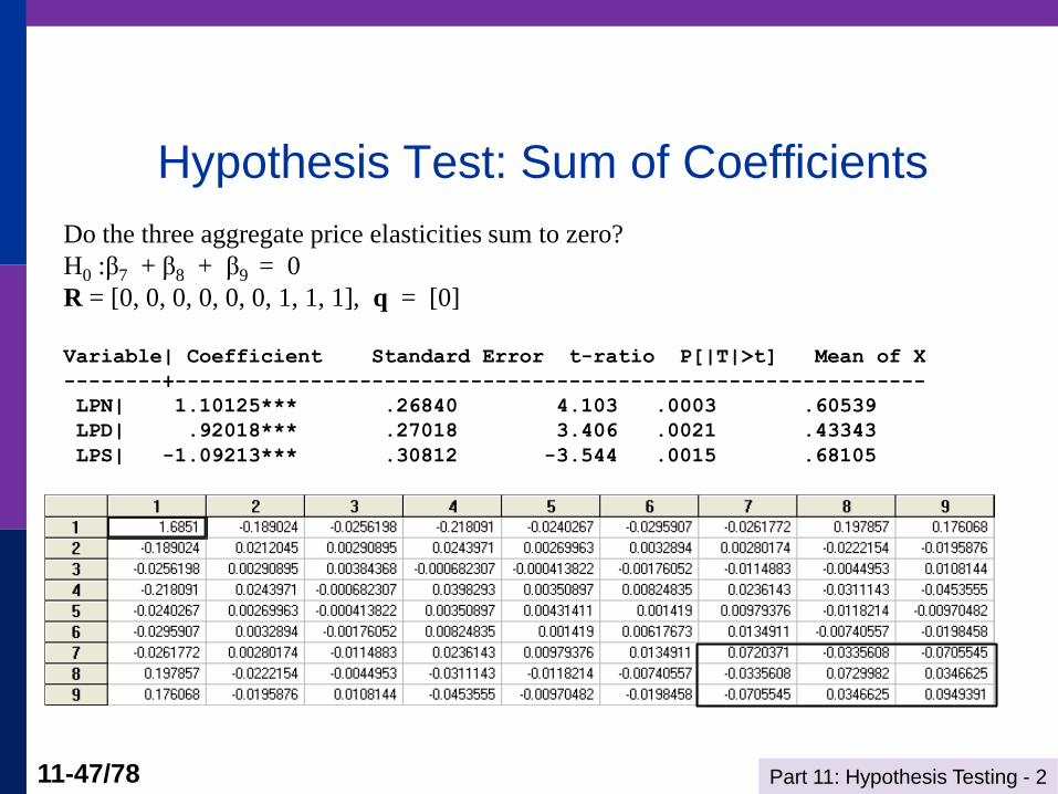
Hypothesis Test: Sum of Coefficients
Do the three aggregate price elasticities sum to zero?
H0 :β7 + β8 + β9 = 0
R = [0, 0, 0, 0, 0, 0, 1, 1, 1], q = [0]
Variable| Coefficient Standard Error t-ratio P[|T|>t] Mean of X
--------+-------------------------------------------------------------
LPN| 1.10125*** .26840 4.103 .0003 .60539
LPD| .92018*** .27018 3.406 .0021 .43343
LPS| -1.09213*** .30812 -3.544 .0015 .68105
Part 11: Hypothesis Testing - 2 11-48/78
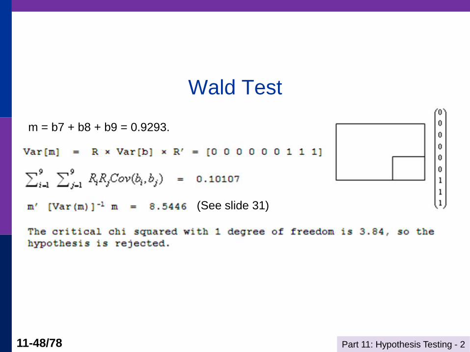
Wald Test
m = b7 + b8 + b9 = 0.9293.
(See slide 31)
Part 11: Hypothesis Testing - 2 11-49/78
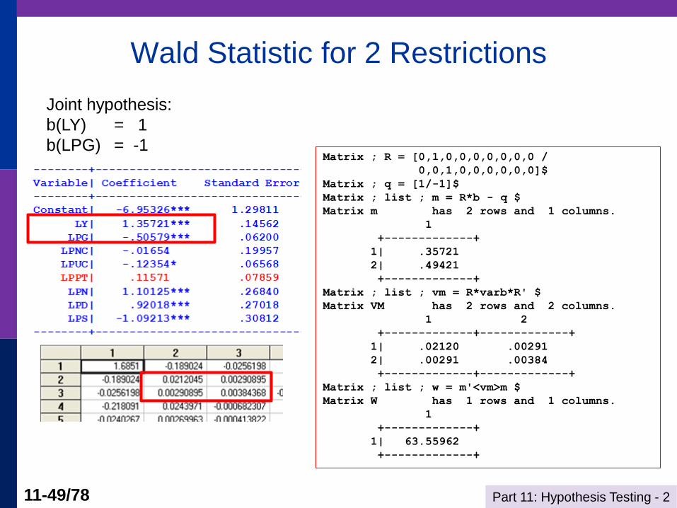
Wald Statistic for 2 Restrictions
Matrix ; R = [0,1,0,0,0,0,0,0,0 /
0,0,1,0,0,0,0,0,0]$
Matrix ; q = [1/-1]$
Matrix ; list ; m = R*b - q $
Matrix m has 2 rows and 1 columns.
1
+-------------+
1| .35721
2| .49421
+-------------+
Matrix ; list ; vm = R*varb*R' $
Matrix VM has 2 rows and 2 columns.
1 2
+-------------+-------------+
1| .02120 .00291
2| .00291 .00384
+-------------+-------------+
Matrix ; list ; w = m'<vm>m $
Matrix W has 1 rows and 1 columns.
1
+-------------+
1| 63.55962
+-------------+
Joint hypothesis:
b(LY) = 1
b(LPG) = -1
Part 11: Hypothesis Testing - 2 11-50/78
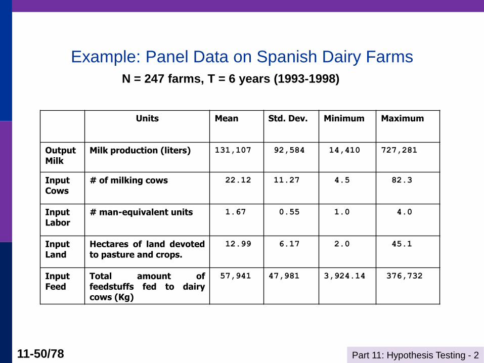
Example: Panel Data on Spanish Dairy Farms
Units Mean Std. Dev. Minimum Maximum
OutputMilk
Milk production (liters) 131,107 92,584 14,410 727,281
Input Cows
# of milking cows 22.12 11.27 4.5 82.3
Input Labor
# man-equivalent units 1.67 0.55 1.0 4.0
Input Land
Hectares of land devoted to pasture and crops.
12.99 6.17 2.0 45.1
Input Feed
Total amount of feedstuffs fed to dairy cows (Kg)
57,941 47,981 3,924.14 376,732
N = 247 farms, T = 6 years (1993-1998)
Part 11: Hypothesis Testing - 2 11-51/78
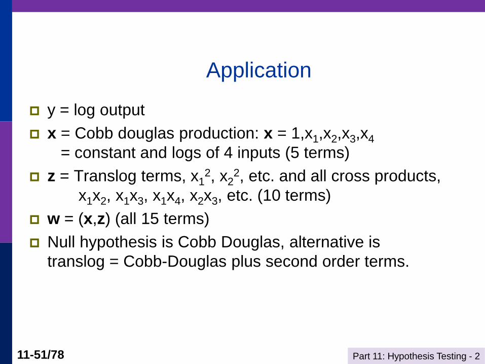
Application
y = log output
x = Cobb douglas production: x = 1,x1,x2,x3,x4
= constant and logs of 4 inputs (5 terms)
z = Translog terms, x12, x2
2, etc. and all cross products,
x1x2, x1x3, x1x4, x2x3, etc. (10 terms)
w = (x,z) (all 15 terms)
Null hypothesis is Cobb Douglas, alternative is
translog = Cobb-Douglas plus second order terms.
Part 11: Hypothesis Testing - 2 11-52/78
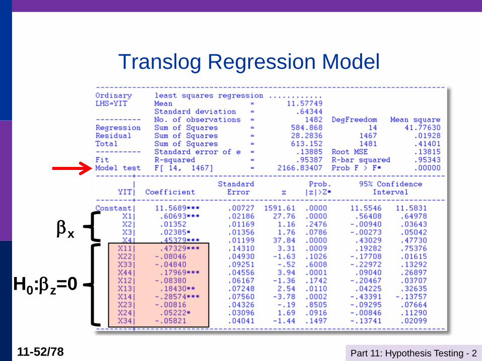
Translog Regression Model
H0:z=0
x
Part 11: Hypothesis Testing - 2 11-53/78
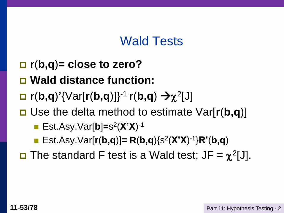
Wald Tests
r(b,q)= close to zero?
Wald distance function:
r(b,q)’{Var[r(b,q)]}-1 r(b,q) 2[J]
Use the delta method to estimate Var[r(b,q)]
Est.Asy.Var[b]=s2(X’X)-1
Est.Asy.Var[r(b,q)]= R(b,q){s2(X’X)-1}R’(b,q)
The standard F test is a Wald test; JF = 2[J].
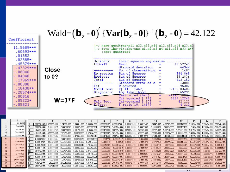
Part 11: Hypothesis Testing - 2 11-54/78
1Wald= { } 42.122 - 0 Var[ - 0] - 0b b bz z z
Close
to 0?
W=J*F
Part 11: Hypothesis Testing - 2 11-55/78
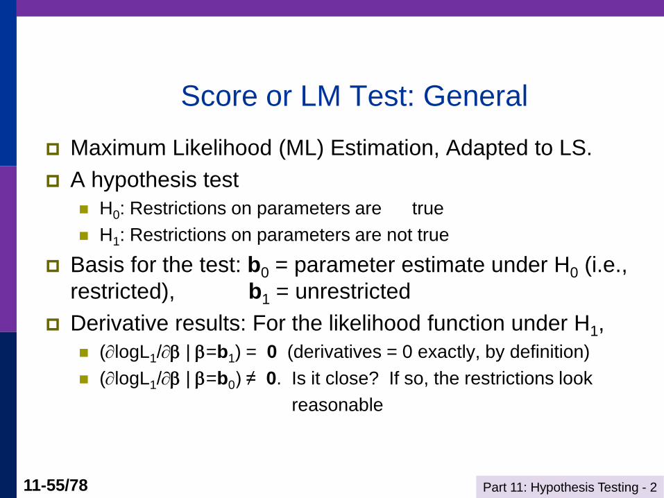
Score or LM Test: General
Maximum Likelihood (ML) Estimation, Adapted to LS.
A hypothesis test
H0: Restrictions on parameters are true
H1: Restrictions on parameters are not true
Basis for the test: b0 = parameter estimate under H0 (i.e.,
restricted), b1 = unrestricted
Derivative results: For the likelihood function under H1,
(logL1/ | =b1) = 0 (derivatives = 0 exactly, by definition)
(logL1/ | =b0) ≠ 0. Is it close? If so, the restrictions look
reasonable
Part 11: Hypothesis Testing - 2 11-56/78
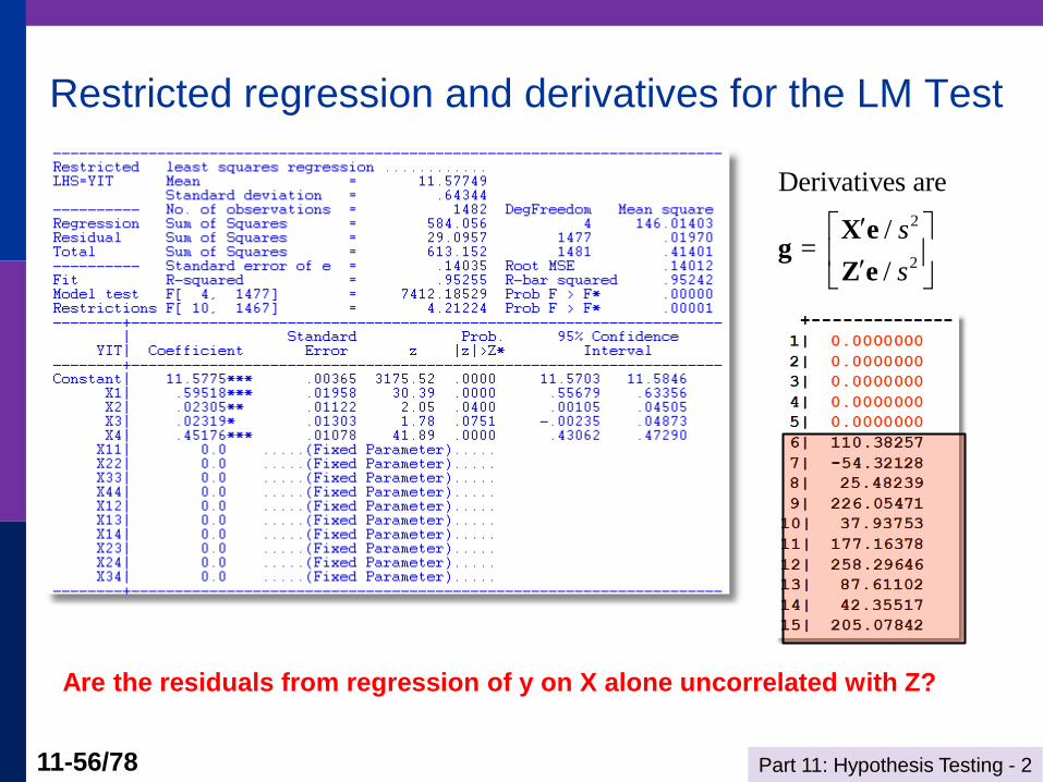
Restricted regression and derivatives for the LM Test
Are the residuals from regression of y on X alone uncorrelated with Z?
2
2
Derivatives are
/ =
/
s
s
X eg
Z e
Part 11: Hypothesis Testing - 2 11-57/78
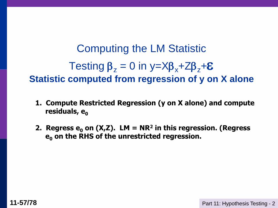
Computing the LM Statistic
Testing z = 0 in y=Xx+Zz+ Statistic computed from regression of y on X alone
1. Compute Restricted Regression (y on X alone) and compute residuals, e0
2. Regress e0 on (X,Z). LM = NR2 in this regression. (Regress e0 on the RHS of the unrestricted regression.
Part 11: Hypothesis Testing - 2 11-58/78
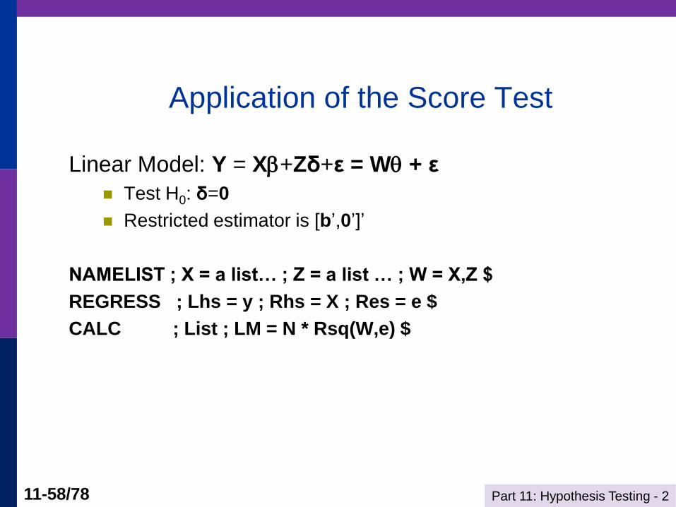
Application of the Score Test
Linear Model: Y = X+Zδ+ε = W + ε
Test H0: δ=0
Restricted estimator is [b’,0’]’
NAMELIST ; X = a list… ; Z = a list … ; W = X,Z $
REGRESS ; Lhs = y ; Rhs = X ; Res = e $
CALC ; List ; LM = N * Rsq(W,e) $
Part 11: Hypothesis Testing - 2 11-59/78
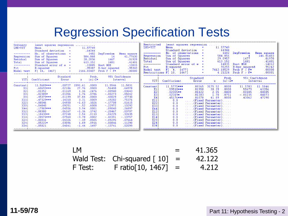
Regression Specification Tests
LM = 41.365 Wald Test: Chi-squared [ 10] = 42.122 F Test: F ratio[10, 1467] = 4.212
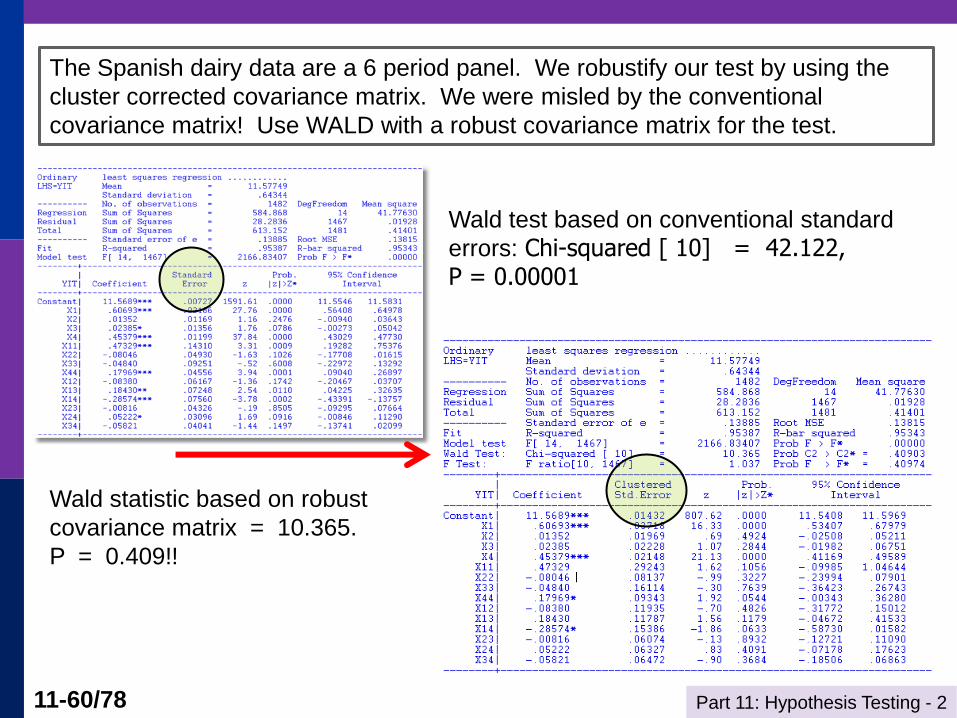
Part 11: Hypothesis Testing - 2 11-60/78
Wald test based on conventional standard
errors: Chi-squared [ 10] = 42.122, P = 0.00001
Wald statistic based on robust
covariance matrix = 10.365.
P = 0.409!!
The Spanish dairy data are a 6 period panel. We robustify our test by using the
cluster corrected covariance matrix. We were misled by the conventional
covariance matrix! Use WALD with a robust covariance matrix for the test.

Part 11: Hypothesis Testing - 2 11-61/78
Structural Change Test
Part 11: Hypothesis Testing - 2 11-62/78
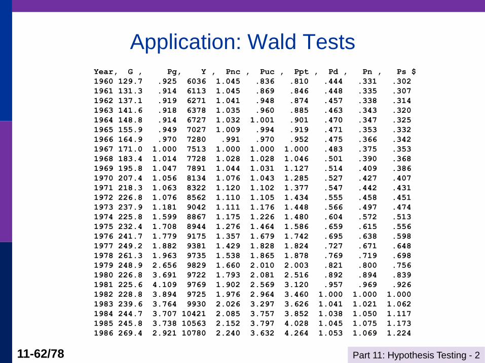
Application: Wald Tests Year, G , Pg, Y , Pnc , Puc , Ppt , Pd , Pn , Ps $
1960 129.7 .925 6036 1.045 .836 .810 .444 .331 .302
1961 131.3 .914 6113 1.045 .869 .846 .448 .335 .307
1962 137.1 .919 6271 1.041 .948 .874 .457 .338 .314
1963 141.6 .918 6378 1.035 .960 .885 .463 .343 .320
1964 148.8 .914 6727 1.032 1.001 .901 .470 .347 .325
1965 155.9 .949 7027 1.009 .994 .919 .471 .353 .332
1966 164.9 .970 7280 .991 .970 .952 .475 .366 .342
1967 171.0 1.000 7513 1.000 1.000 1.000 .483 .375 .353
1968 183.4 1.014 7728 1.028 1.028 1.046 .501 .390 .368
1969 195.8 1.047 7891 1.044 1.031 1.127 .514 .409 .386
1970 207.4 1.056 8134 1.076 1.043 1.285 .527 .427 .407
1971 218.3 1.063 8322 1.120 1.102 1.377 .547 .442 .431
1972 226.8 1.076 8562 1.110 1.105 1.434 .555 .458 .451
1973 237.9 1.181 9042 1.111 1.176 1.448 .566 .497 .474
1974 225.8 1.599 8867 1.175 1.226 1.480 .604 .572 .513
1975 232.4 1.708 8944 1.276 1.464 1.586 .659 .615 .556
1976 241.7 1.779 9175 1.357 1.679 1.742 .695 .638 .598
1977 249.2 1.882 9381 1.429 1.828 1.824 .727 .671 .648
1978 261.3 1.963 9735 1.538 1.865 1.878 .769 .719 .698
1979 248.9 2.656 9829 1.660 2.010 2.003 .821 .800 .756
1980 226.8 3.691 9722 1.793 2.081 2.516 .892 .894 .839
1981 225.6 4.109 9769 1.902 2.569 3.120 .957 .969 .926
1982 228.8 3.894 9725 1.976 2.964 3.460 1.000 1.000 1.000
1983 239.6 3.764 9930 2.026 3.297 3.626 1.041 1.021 1.062
1984 244.7 3.707 10421 2.085 3.757 3.852 1.038 1.050 1.117
1985 245.8 3.738 10563 2.152 3.797 4.028 1.045 1.075 1.173
1986 269.4 2.921 10780 2.240 3.632 4.264 1.053 1.069 1.224
Part 11: Hypothesis Testing - 2 11-63/78
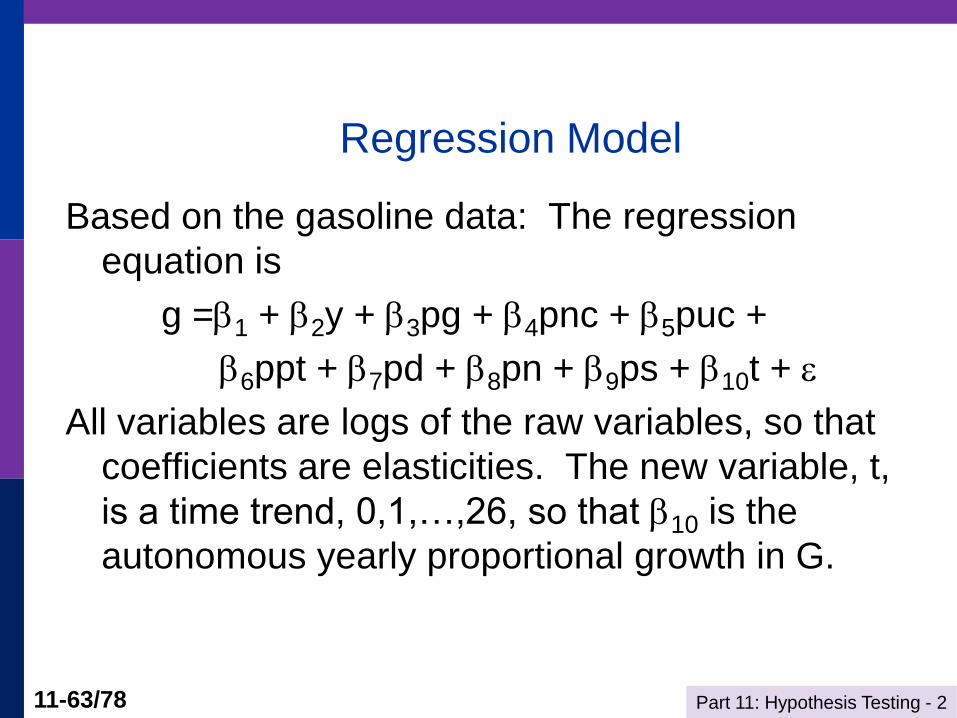
Regression Model
Based on the gasoline data: The regression
equation is
g =1 + 2y + 3pg + 4pnc + 5puc +
6ppt + 7pd + 8pn + 9ps + 10t +
All variables are logs of the raw variables, so that
coefficients are elasticities. The new variable, t,
is a time trend, 0,1,…,26, so that 10 is the
autonomous yearly proportional growth in G.
Part 11: Hypothesis Testing - 2 11-64/78
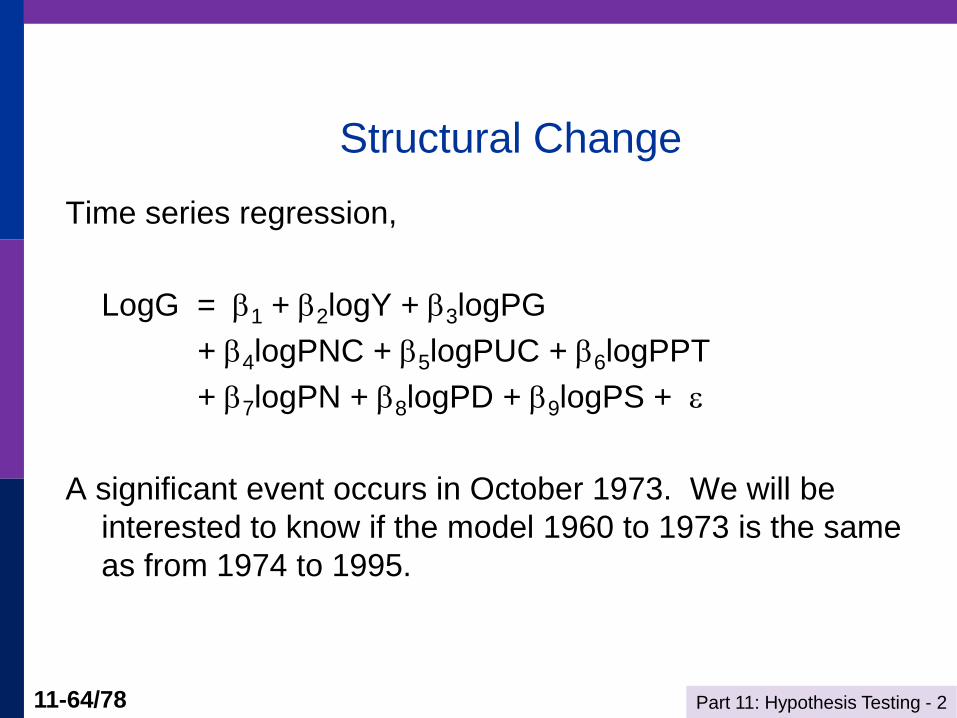
Structural Change
Time series regression,
LogG = 1 + 2logY + 3logPG
+ 4logPNC + 5logPUC + 6logPPT
+ 7logPN + 8logPD + 9logPS +
A significant event occurs in October 1973. We will be
interested to know if the model 1960 to 1973 is the same
as from 1974 to 1995.
Part 11: Hypothesis Testing - 2 11-65/78
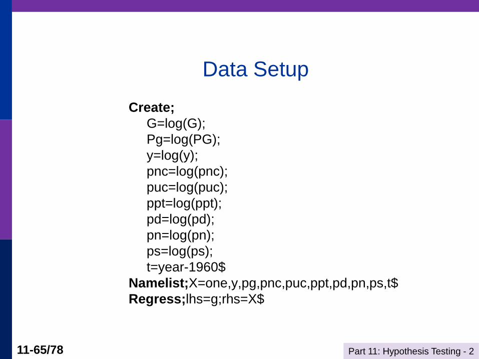
Data Setup
Create;
G=log(G);
Pg=log(PG);
y=log(y);
pnc=log(pnc);
puc=log(puc);
ppt=log(ppt);
pd=log(pd);
pn=log(pn);
ps=log(ps);
t=year-1960$
Namelist;X=one,y,pg,pnc,puc,ppt,pd,pn,ps,t$
Regress;lhs=g;rhs=X$
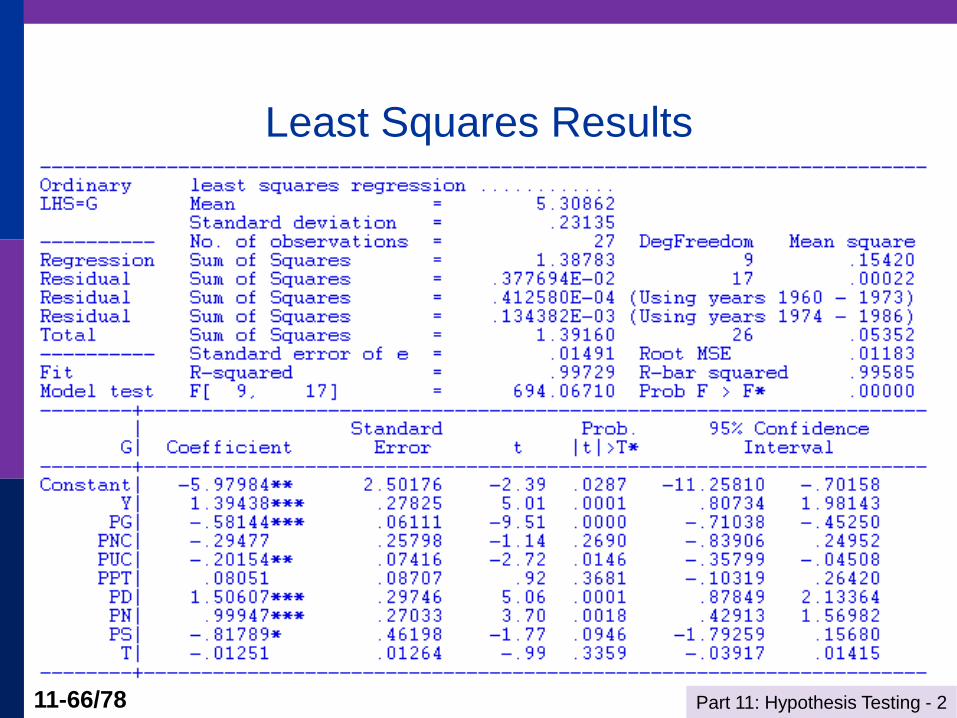
Part 11: Hypothesis Testing - 2 11-66/78
Least Squares Results
Part 11: Hypothesis Testing - 2 11-67/78
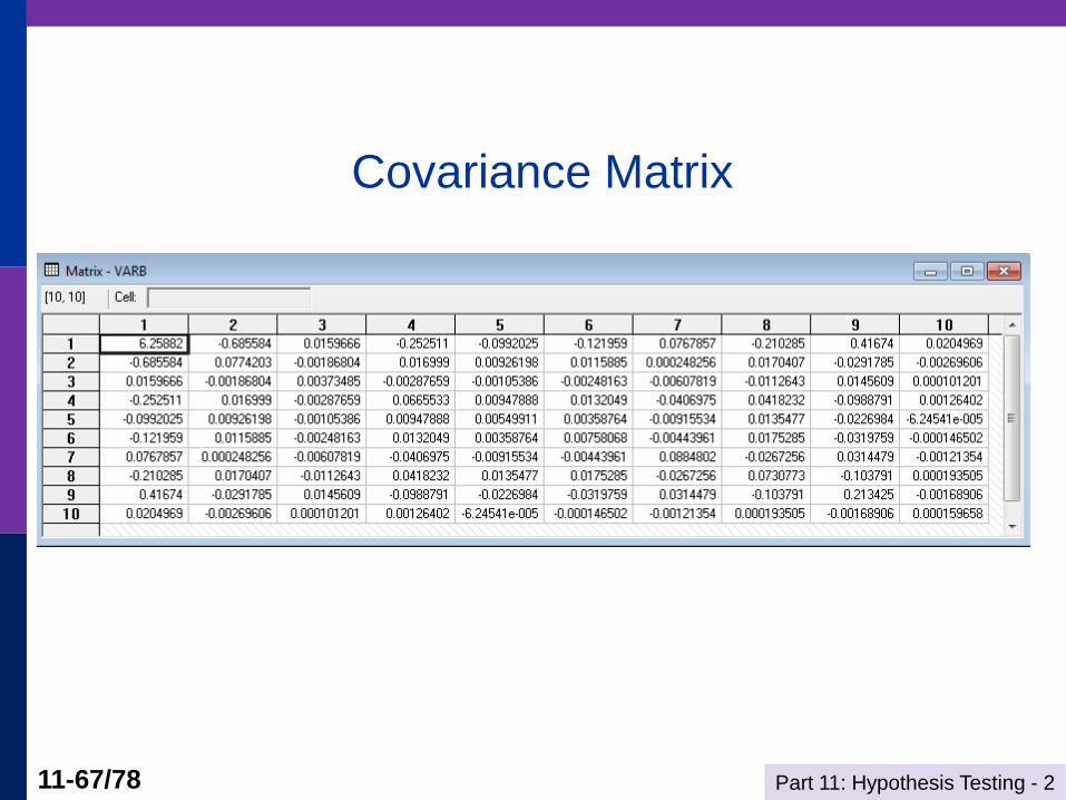
Covariance Matrix
Part 11: Hypothesis Testing - 2 11-68/78
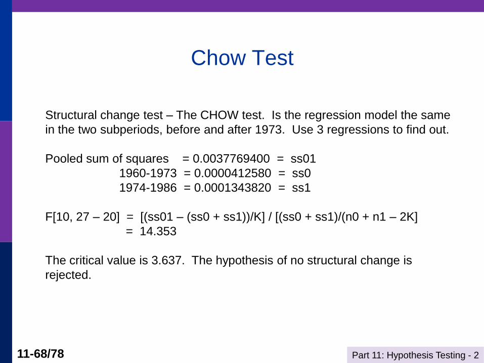
Chow Test
Structural change test – The CHOW test. Is the regression model the same
in the two subperiods, before and after 1973. Use 3 regressions to find out.
Pooled sum of squares = 0.0037769400 = ss01
1960-1973 = 0.0000412580 = ss0
1974-1986 = 0.0001343820 = ss1
F[10, 27 – 20] = [(ss01 – (ss0 + ss1))/K] / [(ss0 + ss1)/(n0 + n1 – 2K]
= 14.353
The critical value is 3.637. The hypothesis of no structural change is
rejected.
Part 11: Hypothesis Testing - 2 11-69/78
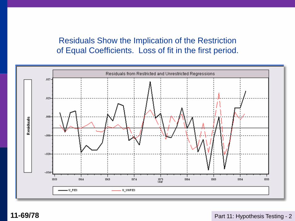
Residuals Show the Implication of the Restriction
of Equal Coefficients. Loss of fit in the first period.
Part 11: Hypothesis Testing - 2 11-70/78
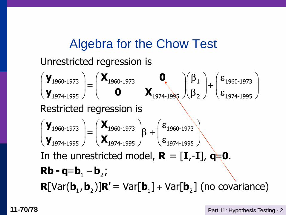
Algebra for the Chow Test
1960-1973 1960-1973 1960-19731
1974-1995 1974-1995 1974-19952
1960-1973 1960-1973 19
1974-1995 1974-1995
Unrestricted regression is
Restricted regression is
y X 0
y 0 X
y X
y X
60-1973
1974-1995
1 2
1 2 1 2
In the unrestricted model, = [ ,- ], = .
= ;
[Var( , )] = Var[ ] Var[ ] (no covariance)
R I I q 0
Rb - q b b
R b b R' b b
Part 11: Hypothesis Testing - 2 11-71/78
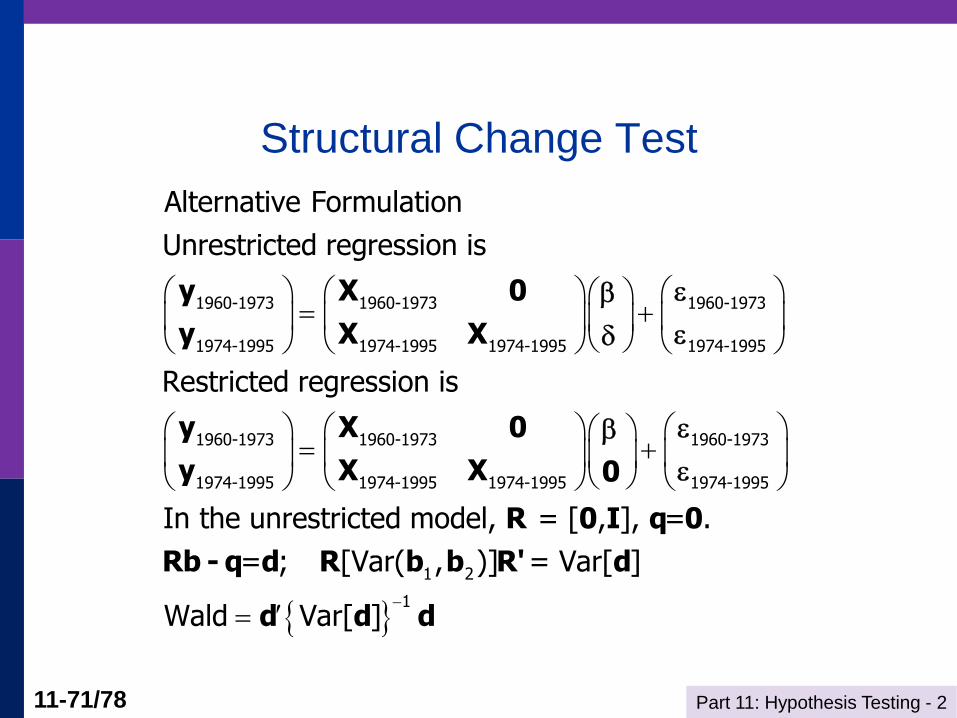
Structural Change Test
1960-1973 1960-1973 1960-1973
1974-1995 1974-1995 1974-1995 1974-1995
1960-1973
1974-1995
Alternative Formulation
Unrestricted regression is
Restricted regression is
y X 0
y X X
y X
y
1960-1973 1960-1973
1974-1995 1974-1995 1974-1995
1 2
1
In the unrestricted model, = [ , ], = .
= ; [Var( , )] = Var[ ]
Wald Var[ ]
0
X X 0
R 0 I q 0
Rb - q d R b b R' d
d d d

Part 11: Hypothesis Testing - 2 11-72/78
Application – Health and Income
German Health Care Usage Data, 7,293 Individuals, Varying Numbers of Periods
Variables in the file are
Data downloaded from Journal of Applied Econometrics Archive. This is an unbalanced
panel with 7,293 individuals. There are altogether 27,326 observations. The number of
observations ranges from 1 to 7 per family. (Frequencies are: 1=1525, 2=2158, 3=825,
4=926, 5=1051, 6=1000, 7=987). The dependent variable of interest is
DOCVIS = number of visits to the doctor in the observation period
HHNINC = household nominal monthly net income in German marks / 10000.
(4 observations with income=0 were dropped)
HHKIDS = children under age 16 in the household = 1; otherwise = 0
EDUC = years of schooling
AGE = age in years
MARRIED=marital status
WHITEC = 1 if has “white collar” job
Part 11: Hypothesis Testing - 2 11-73/78
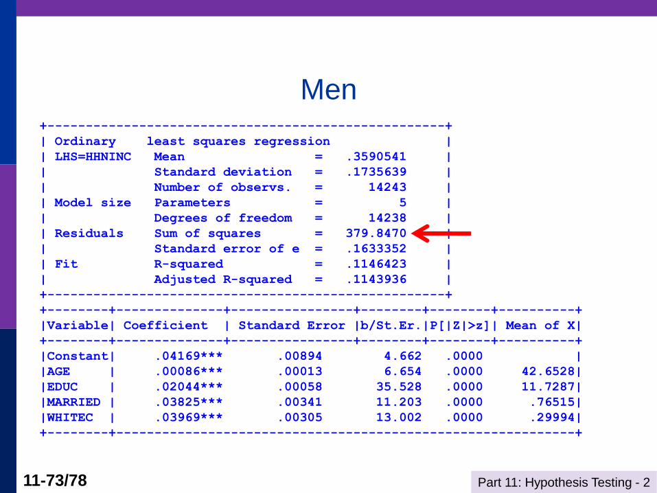
Men +----------------------------------------------------+
| Ordinary least squares regression |
| LHS=HHNINC Mean = .3590541 |
| Standard deviation = .1735639 |
| Number of observs. = 14243 |
| Model size Parameters = 5 |
| Degrees of freedom = 14238 |
| Residuals Sum of squares = 379.8470 |
| Standard error of e = .1633352 |
| Fit R-squared = .1146423 |
| Adjusted R-squared = .1143936 |
+----------------------------------------------------+
+--------+--------------+----------------+--------+--------+----------+
|Variable| Coefficient | Standard Error |b/St.Er.|P[|Z|>z]| Mean of X|
+--------+--------------+----------------+--------+--------+----------+
|Constant| .04169*** .00894 4.662 .0000 |
|AGE | .00086*** .00013 6.654 .0000 42.6528|
|EDUC | .02044*** .00058 35.528 .0000 11.7287|
|MARRIED | .03825*** .00341 11.203 .0000 .76515|
|WHITEC | .03969*** .00305 13.002 .0000 .29994|
+--------+------------------------------------------------------------+

Part 11: Hypothesis Testing - 2 11-74/78
Women
+----------------------------------------------------+
| Ordinary least squares regression |
| LHS=HHNINC Mean = .3444951 |
| Standard deviation = .1801790 |
| Number of observs. = 13083 |
| Model size Parameters = 5 |
| Degrees of freedom = 13078 |
| Residuals Sum of squares = 363.8789 |
| Standard error of e = .1668045 |
| Fit R-squared = .1432098 |
| Adjusted R-squared = .1429477 |
+----------------------------------------------------+
+--------+--------------+----------------+--------+--------+----------+
|Variable| Coefficient | Standard Error |b/St.Er.|P[|Z|>z]| Mean of X|
+--------+--------------+----------------+--------+--------+----------+
|Constant| .01191 .01158 1.029 .3036 |
|AGE | .00026* .00014 1.875 .0608 44.4760|
|EDUC | .01941*** .00072 26.803 .0000 10.8764|
|MARRIED | .12081*** .00343 35.227 .0000 .75151|
|WHITEC | .06445*** .00334 19.310 .0000 .29924|
+--------+------------------------------------------------------------+
Part 11: Hypothesis Testing - 2 11-75/78
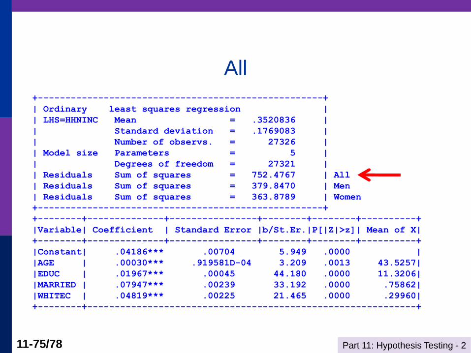
All
+----------------------------------------------------+
| Ordinary least squares regression |
| LHS=HHNINC Mean = .3520836 |
| Standard deviation = .1769083 |
| Number of observs. = 27326 |
| Model size Parameters = 5 |
| Degrees of freedom = 27321 |
| Residuals Sum of squares = 752.4767 | All
| Residuals Sum of squares = 379.8470 | Men
| Residuals Sum of squares = 363.8789 | Women
+----------------------------------------------------+
+--------+--------------+----------------+--------+--------+----------+
|Variable| Coefficient | Standard Error |b/St.Er.|P[|Z|>z]| Mean of X|
+--------+--------------+----------------+--------+--------+----------+
|Constant| .04186*** .00704 5.949 .0000 |
|AGE | .00030*** .919581D-04 3.209 .0013 43.5257|
|EDUC | .01967*** .00045 44.180 .0000 11.3206|
|MARRIED | .07947*** .00239 33.192 .0000 .75862|
|WHITEC | .04819*** .00225 21.465 .0000 .29960|
+--------+------------------------------------------------------------+
Part 11: Hypothesis Testing - 2 11-76/78
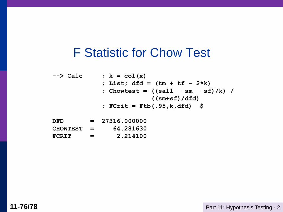
F Statistic for Chow Test
--> Calc ; k = col(x)
; List; dfd = (tm + tf - 2*k)
; Chowtest = ((sall - sm - sf)/k) /
((sm+sf)/dfd)
; FCrit = Ftb(.95,k,dfd) $
DFD = 27316.000000
CHOWTEST = 64.281630
FCRIT = 2.214100
Part 11: Hypothesis Testing - 2 11-77/78
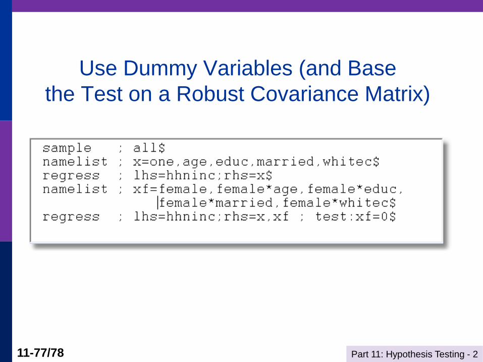
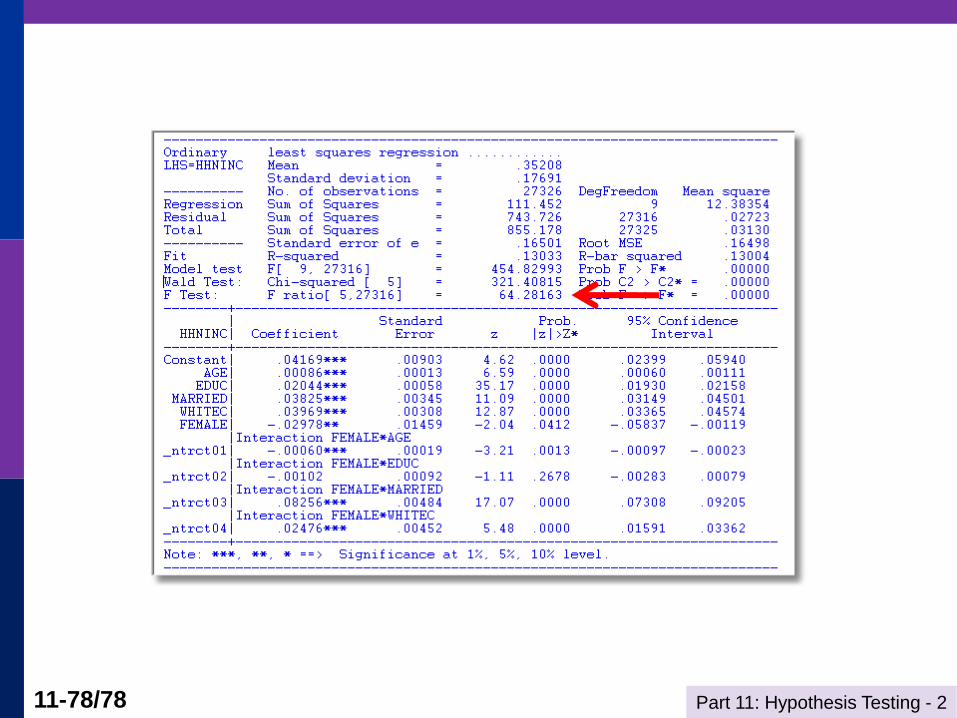
Use Dummy Variables (and Base
the Test on a Robust Covariance Matrix)
Part 11: Hypothesis Testing - 2 11-78/78
Wald Test for Difference
Part 11: Hypothesis Testing - 2 11-79/78
Specification Test: Normality of
Specification test for distribution
Standard tests:
Kolmogorov-Smirnov: compare empirical cdf of X to normal with
same mean and variance
Bowman-Shenton: Compare third and fourth moments of X to
normal, 0 (no skewness) and 34 (meso kurtosis)
Bera-Jarque – adapted Bowman/Shenton to linear
regression residuals
Part 11: Hypothesis Testing - 2 11-80/78
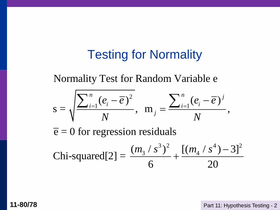
Testing for Normality
2
1 1
3 2 4 2
3 4
Normality Test for Random Variable e
( ) ( )s = , m ,
e = 0 for regression residuals
( / ) [( / ) 3]Chi-squared[2] =
6 20
n n j
i ii ij
e e e e
N N
m s m s
Part 11: Hypothesis Testing - 2 11-81/78
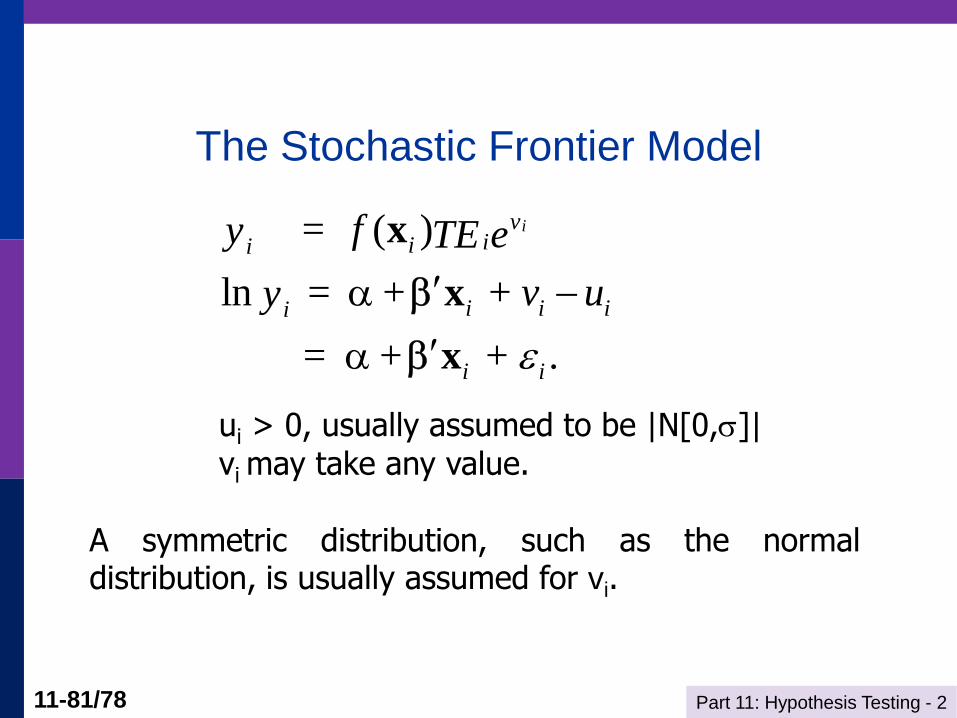
The Stochastic Frontier Model
( )
ln +
= + .
iviii
i i ii
i i
= fy eTE
= + v uy
+
x
x
x
ui > 0, usually assumed to be |N[0,]| vi may take any value. A symmetric distribution, such as the normal distribution, is usually assumed for vi.
Part 11: Hypothesis Testing - 2 11-82/78
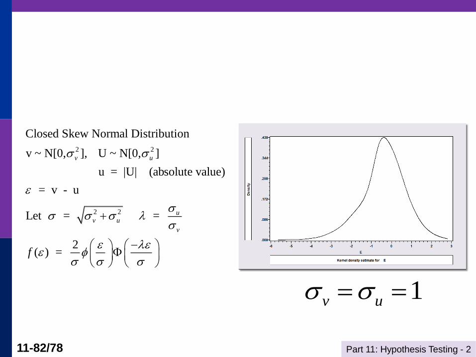
2 2
2 2
Closed Skew Normal Distribution
v ~ N[0, ], U ~ N[0, ]
u = |U| (absolute value)
= v - u
Let = =
2( ) =
v u
uv u
v
f
1v u
Part 11: Hypothesis Testing - 2 11-83/78
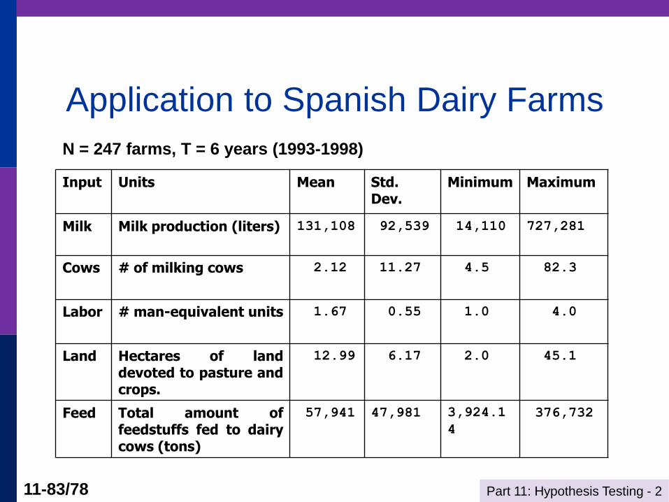
Application to Spanish Dairy Farms
Input Units Mean Std. Dev.
Minimum Maximum
Milk Milk production (liters) 131,108 92,539 14,110 727,281
Cows # of milking cows 2.12 11.27 4.5 82.3
Labor # man-equivalent units 1.67 0.55 1.0 4.0
Land Hectares of land devoted to pasture and crops.
12.99 6.17 2.0 45.1
Feed Total amount of feedstuffs fed to dairy cows (tons)
57,941 47,981 3,924.1
4
376,732
N = 247 farms, T = 6 years (1993-1998)
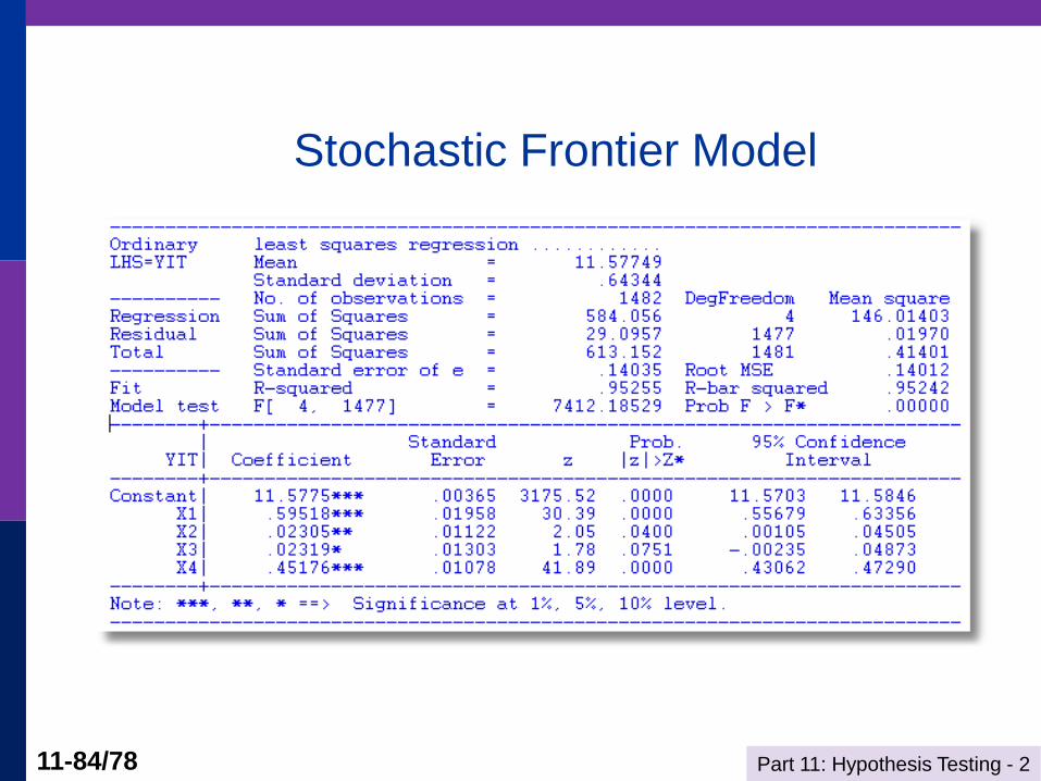
Part 11: Hypothesis Testing - 2 11-84/78
Stochastic Frontier Model
Part 11: Hypothesis Testing - 2 11-85/78
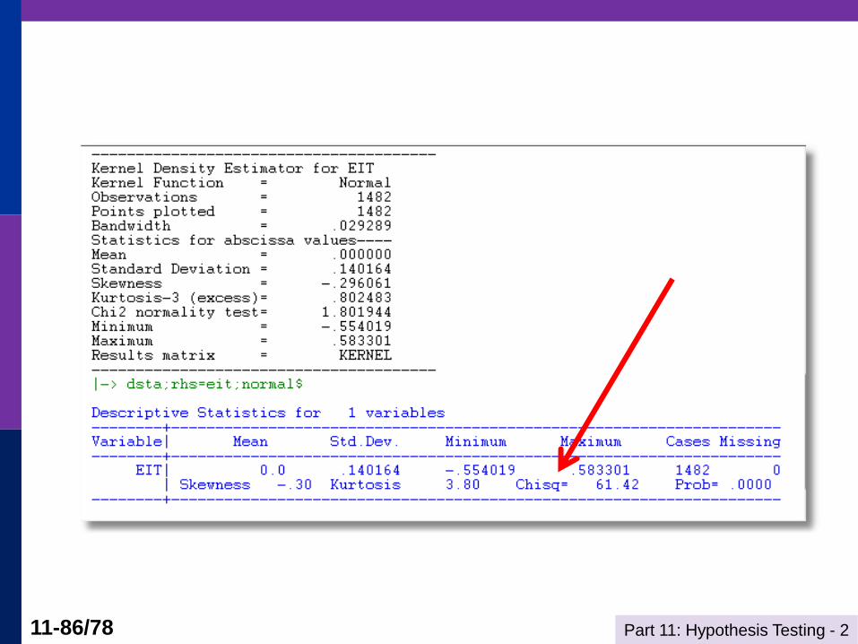
Part 11: Hypothesis Testing - 2 11-86/78
Part 11: Hypothesis Testing - 2 11-87/78
Appendix
Miscellaneous Results
Part 11: Hypothesis Testing - 2 11-88/78
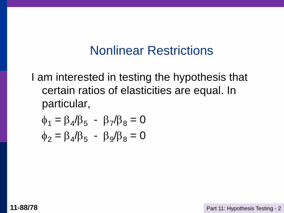
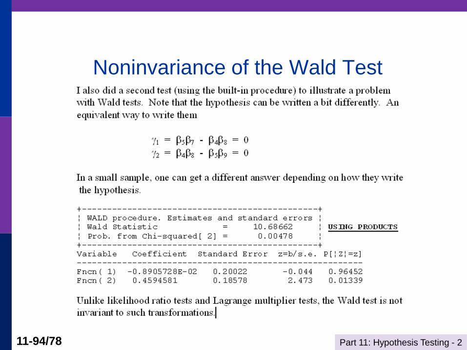
Nonlinear Restrictions
I am interested in testing the hypothesis that
certain ratios of elasticities are equal. In
particular,
1 = 4/5 - 7/8 = 0
2 = 4/5 - 9/8 = 0
Part 11: Hypothesis Testing - 2 11-89/78
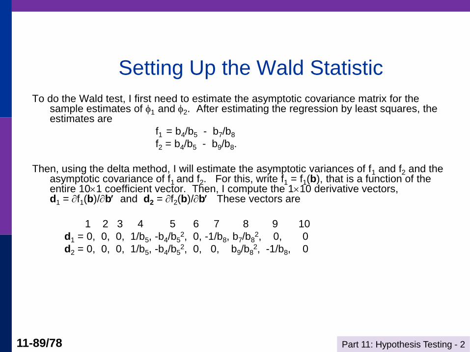
Setting Up the Wald Statistic
To do the Wald test, I first need to estimate the asymptotic covariance matrix for the sample estimates of 1 and 2. After estimating the regression by least squares, the estimates are
f1 = b4/b5 - b7/b8
f2 = b4/b5 - b9/b8.
Then, using the delta method, I will estimate the asymptotic variances of f1 and f2 and the asymptotic covariance of f1 and f2. For this, write f1 = f1(b), that is a function of the entire 101 coefficient vector. Then, I compute the 110 derivative vectors, d1 = f1(b)/b and d2 = f2(b)/b These vectors are
1 2 3 4 5 6 7 8 9 10
d1 = 0, 0, 0, 1/b5, -b4/b52, 0, -1/b8, b7/b8
2, 0, 0
d2 = 0, 0, 0, 1/b5, -b4/b52, 0, 0, b9/b8
2, -1/b8, 0
Part 11: Hypothesis Testing - 2 11-90/78
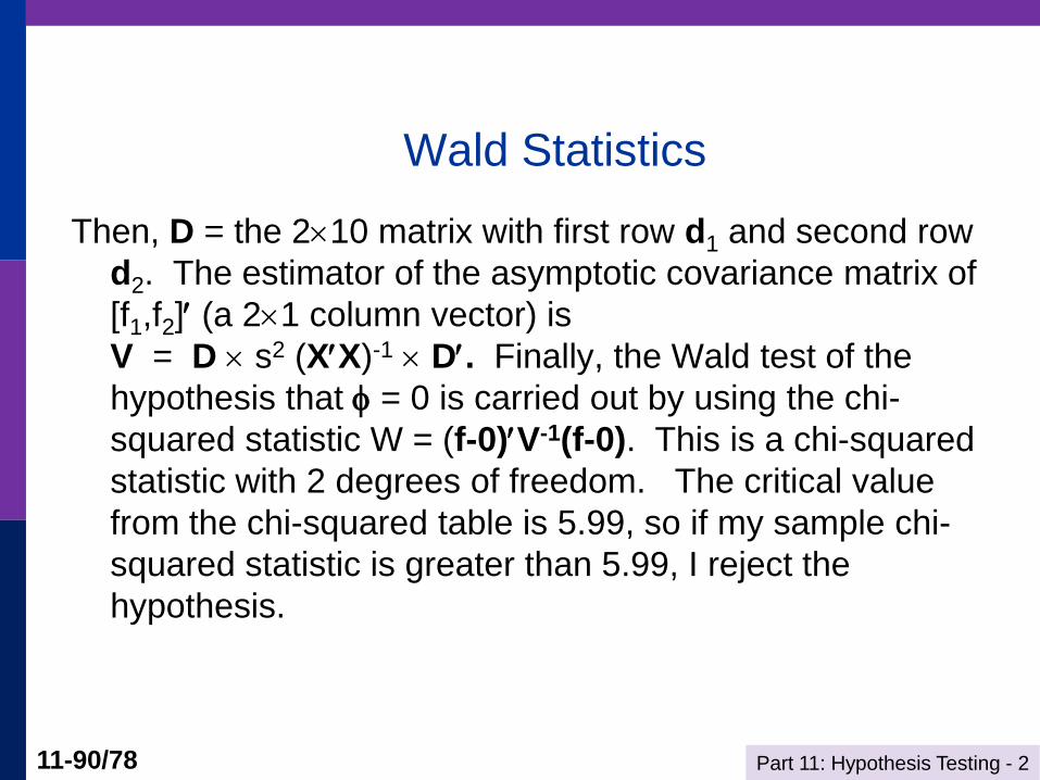
Wald Statistics
Then, D = the 210 matrix with first row d1 and second row
d2. The estimator of the asymptotic covariance matrix of
[f1,f2] (a 21 column vector) is
V = D s2 (XX)-1 D. Finally, the Wald test of the
hypothesis that = 0 is carried out by using the chi-
squared statistic W = (f-0)V-1(f-0). This is a chi-squared
statistic with 2 degrees of freedom. The critical value
from the chi-squared table is 5.99, so if my sample chi-
squared statistic is greater than 5.99, I reject the
hypothesis.
Part 11: Hypothesis Testing - 2 11-91/78
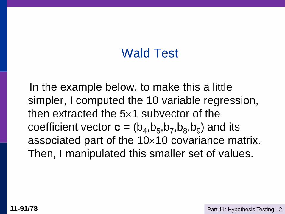
Wald Test
In the example below, to make this a little
simpler, I computed the 10 variable regression,
then extracted the 51 subvector of the
coefficient vector c = (b4,b5,b7,b8,b9) and its
associated part of the 1010 covariance matrix.
Then, I manipulated this smaller set of values.
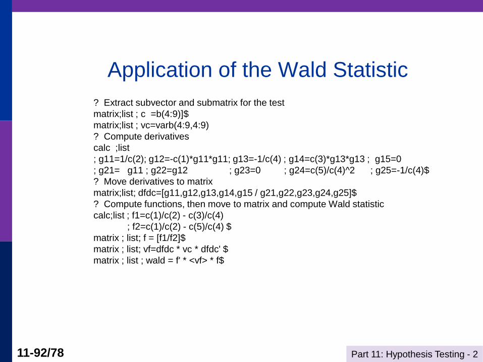
Part 11: Hypothesis Testing - 2 11-92/78
Application of the Wald Statistic
? Extract subvector and submatrix for the test
matrix;list ; c =b(4:9)]$
matrix;list ; vc=varb(4:9,4:9)
? Compute derivatives
calc ;list
; g11=1/c(2); g12=-c(1)*g11*g11; g13=-1/c(4) ; g14=c(3)*g13*g13 ; g15=0
; g21= g11 ; g22=g12 ; g23=0 ; g24=c(5)/c(4)^2 ; g25=-1/c(4)$
? Move derivatives to matrix
matrix;list; dfdc=[g11,g12,g13,g14,g15 / g21,g22,g23,g24,g25]$
? Compute functions, then move to matrix and compute Wald statistic
calc;list ; f1=c(1)/c(2) - c(3)/c(4)
; f2=c(1)/c(2) - c(5)/c(4) $
matrix ; list; f = [f1/f2]$
matrix ; list; vf=dfdc * vc * dfdc' $
matrix ; list ; wald = f' * <vf> * f$
Part 11: Hypothesis Testing - 2 11-93/78
Computations Matrix C is 5 rows by 1 columns.
1
1 -0.2948 -0.2015 1.506 0.9995 -0.8179
Matrix VC is 5 rows by 5 columns.
1 2 3 4 5
1 0.6655E-01 0.9479E-02 -0.4070E-01 0.4182E-01 -0.9888E-01
2 0.9479E-02 0.5499E-02 -0.9155E-02 0.1355E-01 -0.2270E-01
3 -0.4070E-01 -0.9155E-02 0.8848E-01 -0.2673E-01 0.3145E-01
4 0.4182E-01 0.1355E-01 -0.2673E-01 0.7308E-01 -0.1038
5 -0.9888E-01 -0.2270E-01 0.3145E-01 -0.1038 0.2134
G11 = -4.96184 G12 = 7.25755 G13= -1.00054 G14 = 1.50770 G15 = 0.000000
G21 = -4.96184 G22 = 7.25755 G23 = 0 G24 = -0.818753 G25 = -1.00054
DFDC=[G11,G12,G13,G14,G15/G21,G22,G23,G24,G25]
Matrix DFDC is 2 rows by 5 columns.
1 2 3 4 5
1 -4.962 7.258 -1.001 1.508 0.0000
2 -4.962 7.258 0.0000 -0.8188 -1.001
F1= -0.442126E-01
F2= 2.28098
F=[F1/F2]
VF=DFDC*VC*DFDC'
Matrix VF is 2 rows by 2 columns.
1 2
1 0.9804 0.7846
2 0.7846 0.8648
WALD Matrix Result is 1 rows by 1 columns.
1
1 22.65
Part 11: Hypothesis Testing - 2 11-94/78
Noninvariance of the Wald Test
Part 11: Hypothesis Testing - 2 11-95/78
Nonnested Regression Models
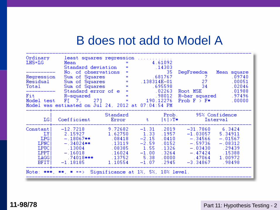
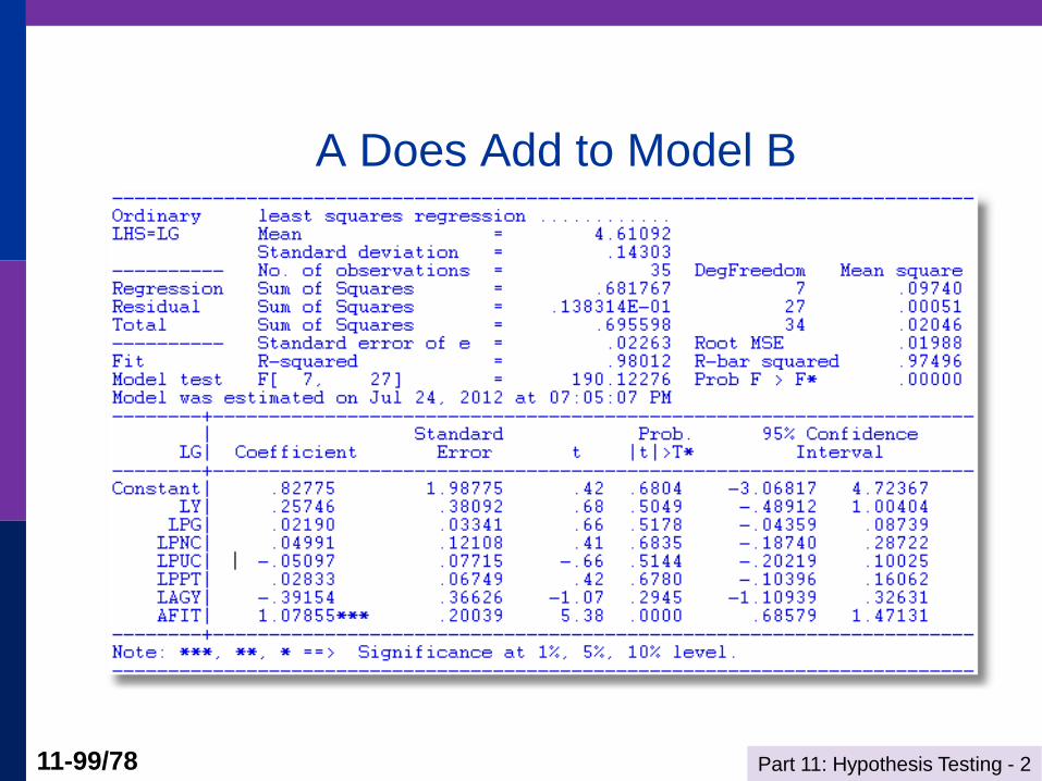
Davidson and MacKinnon: If model A is correct,
then predictions from model B will not add to the
fit of model A to the data.
Vuong: If model A is correct, then the likelihood
function will generally favor model A and not
model B
Part 11: Hypothesis Testing - 2 11-96/78
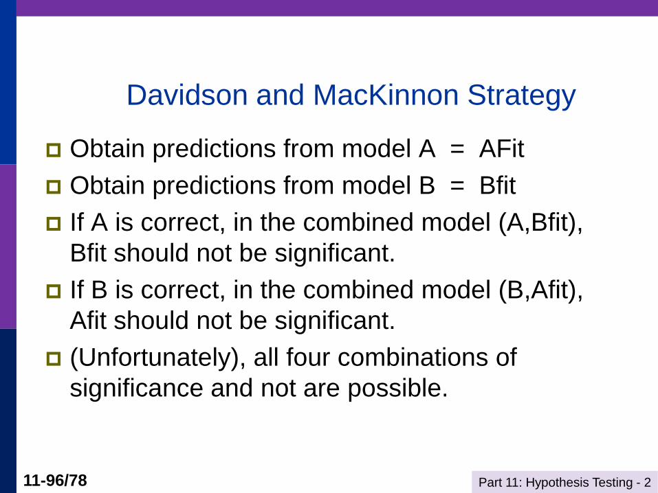
Davidson and MacKinnon Strategy
Obtain predictions from model A = AFit
Obtain predictions from model B = Bfit
If A is correct, in the combined model (A,Bfit),
Bfit should not be significant.
If B is correct, in the combined model (B,Afit),
Afit should not be significant.
(Unfortunately), all four combinations of
significance and not are possible.
Part 11: Hypothesis Testing - 2 11-97/78
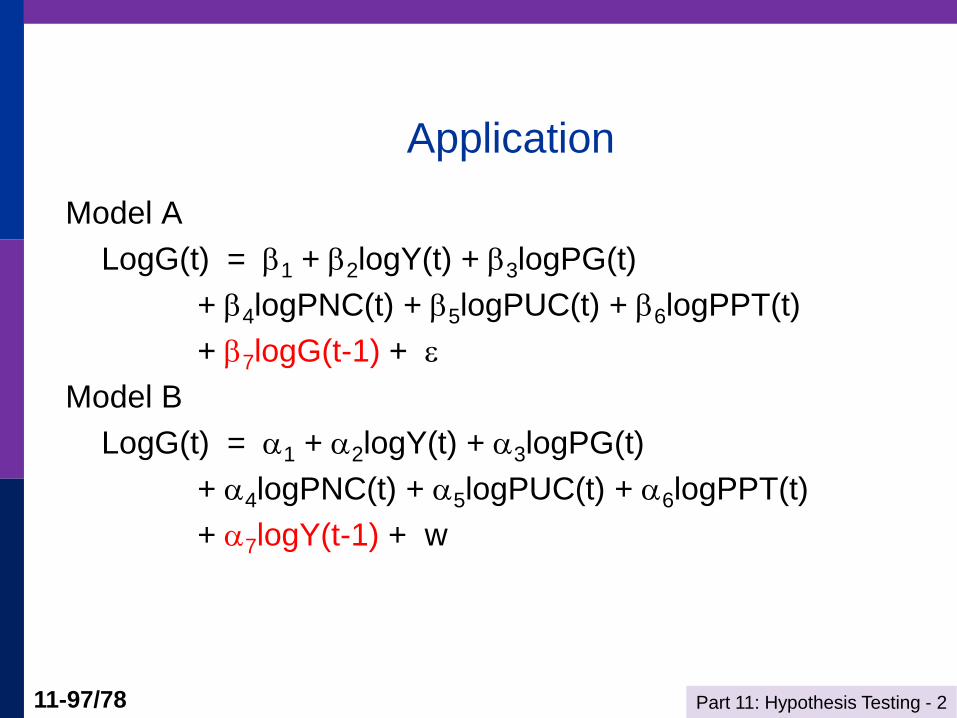
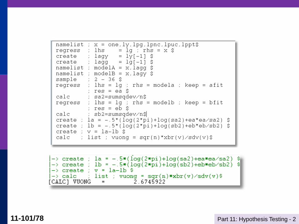
Application
Model A
LogG(t) = 1 + 2logY(t) + 3logPG(t)
+ 4logPNC(t) + 5logPUC(t) + 6logPPT(t)
+ 7logG(t-1) +
Model B
LogG(t) = 1 + 2logY(t) + 3logPG(t)
+ 4logPNC(t) + 5logPUC(t) + 6logPPT(t)
+ 7logY(t-1) + w
Part 11: Hypothesis Testing - 2 11-98/78
B does not add to Model A
Part 11: Hypothesis Testing - 2 11-99/78
A Does Add to Model B
Part 11: Hypothesis Testing - 2 11-100/78
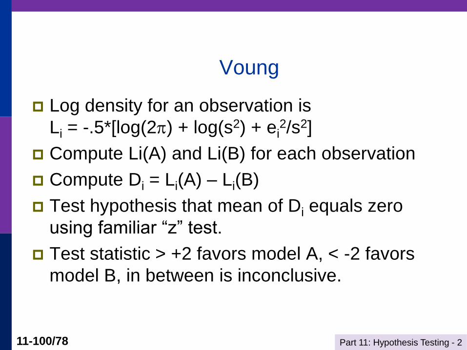
Voung
Log density for an observation is
Li = -.5*[log(2) + log(s2) + ei2/s2]
Compute Li(A) and Li(B) for each observation
Compute Di = Li(A) – Li(B)
Test hypothesis that mean of Di equals zero
using familiar “z” test.
Test statistic > +2 favors model A, < -2 favors
model B, in between is inconclusive.
Part 11: Hypothesis Testing - 2 11-101/78
Part 11: Hypothesis Testing - 2 11-102/78
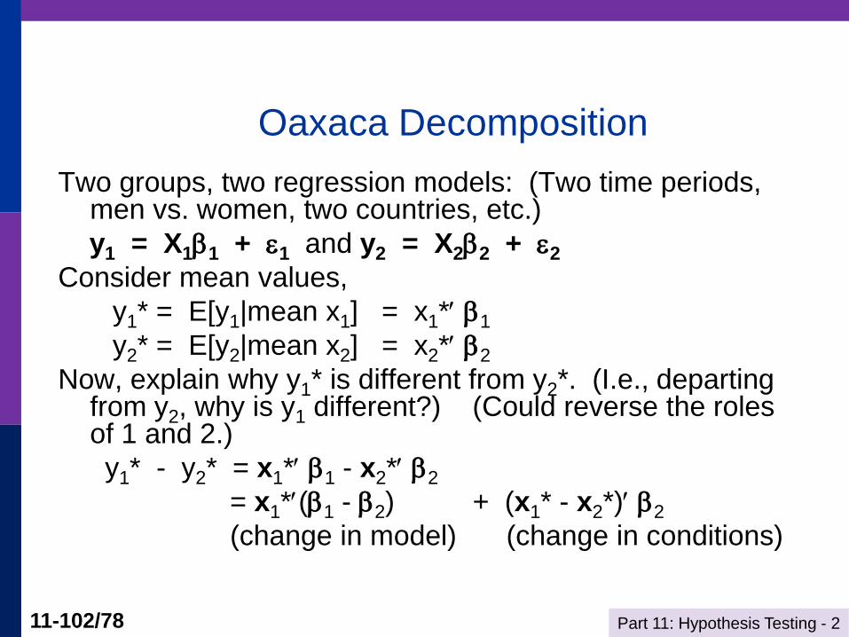
Oaxaca Decomposition
Two groups, two regression models: (Two time periods, men vs. women, two countries, etc.)
y1 = X11 + 1 and y2 = X22 + 2
Consider mean values,
y1* = E[y1|mean x1] = x1* 1
y2* = E[y2|mean x2] = x2* 2
Now, explain why y1* is different from y2*. (I.e., departing from y2, why is y1 different?) (Could reverse the roles of 1 and 2.)
y1* - y2* = x1* 1 - x2* 2
= x1*(1 - 2) + (x1* - x2*) 2
(change in model) (change in conditions)
Part 11: Hypothesis Testing - 2 11-103/78
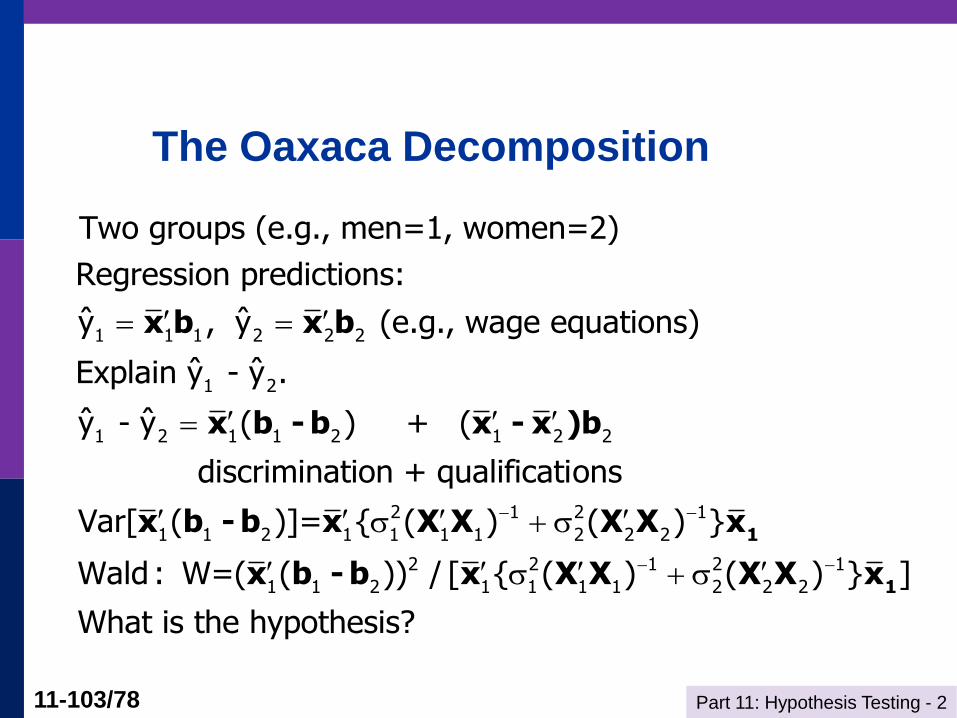
The Oaxaca Decomposition
1 1 1 2 2 2
1 2
1 2 1 1 2 1 2 2
Two groups (e.g., men=1, women=2)
Regression predictions:
ˆ ˆy , y (e.g., wage equations)
ˆ ˆExplain y - y .
ˆ ˆy - y ( ) + (
discrimination + qualificati
x b x b
x b - b x - x )b
2 1 2 1
1 1 2 1 1 1 1 2 2 2
2 2 1 2 1
1 1 2 1 1 1 1 2 2 2
ons
Var[ ( )]= { ( ) ( ) }
Wald : W=( ( )) / [ { ( ) ( ) } ]
What is the hypothesis?
1
1
x b - b x X X X X x
x b - b x X X X X x
Part 11: Hypothesis Testing - 2 11-104/78
Application - Income German Health Care Usage Data, 7,293 Individuals, Varying Numbers of
Periods
Variables in the file are
Data downloaded from Journal of Applied Econometrics Archive. This is an
unbalanced panel with 7,293 individuals. They can be used for regression, count
models, binary choice, ordered choice, and bivariate binary choice. This is a
large data set. There are altogether 27,326 observations. The number of
observations ranges from 1 to 7. (Frequencies are: 1=1525, 2=2158, 3=825,
4=926, 5=1051, 6=1000, 7=987).
HHNINC = household nominal monthly net income in German marks / 10000.
(4 observations with income=0 were dropped)
HHKIDS = children under age 16 in the household = 1; otherwise = 0
EDUC = years of schooling
AGE = age in years
MARRIED = 1 if married, 0 if not
FEMALE = 1 if female, 0 if male
Part 11: Hypothesis Testing - 2 11-105/78
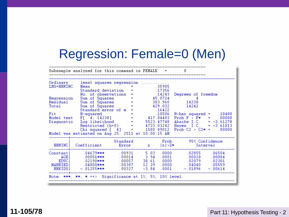
Regression: Female=0 (Men)
Part 11: Hypothesis Testing - 2 11-106/78
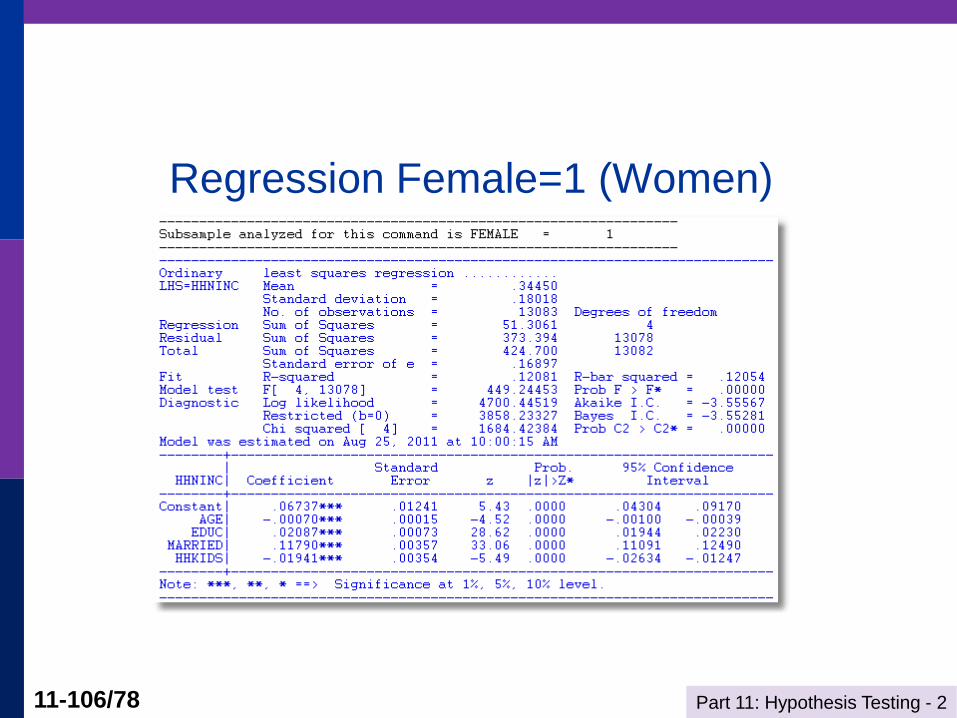
Regression Female=1 (Women)
Part 11: Hypothesis Testing - 2 11-107/78
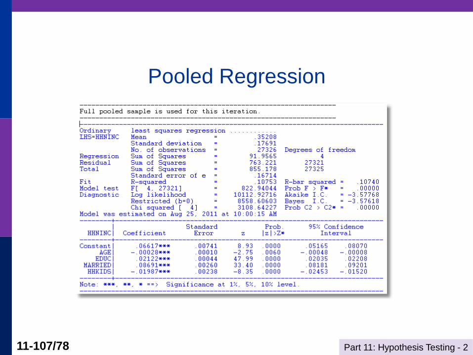
Pooled Regression
Part 11: Hypothesis Testing - 2 11-108/78
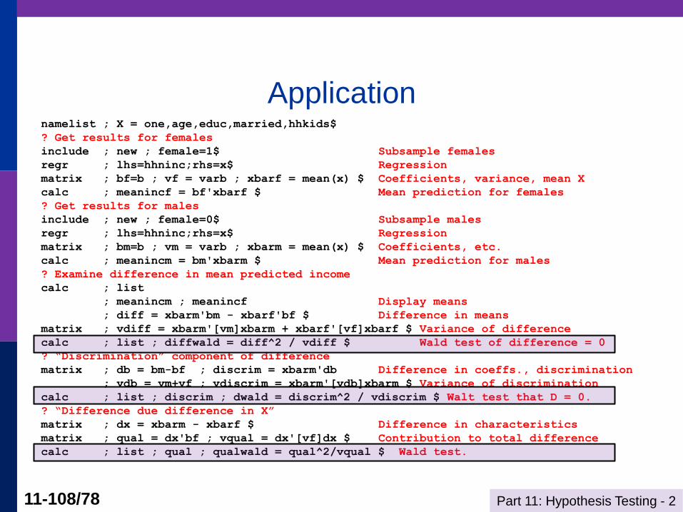
Application namelist ; X = one,age,educ,married,hhkids$
? Get results for females
include ; new ; female=1$ Subsample females
regr ; lhs=hhninc;rhs=x$ Regression
matrix ; bf=b ; vf = varb ; xbarf = mean(x) $ Coefficients, variance, mean X
calc ; meanincf = bf'xbarf $ Mean prediction for females
? Get results for males
include ; new ; female=0$ Subsample males
regr ; lhs=hhninc;rhs=x$ Regression
matrix ; bm=b ; vm = varb ; xbarm = mean(x) $ Coefficients, etc.
calc ; meanincm = bm'xbarm $ Mean prediction for males
? Examine difference in mean predicted income
calc ; list
; meanincm ; meanincf Display means
; diff = xbarm'bm - xbarf'bf $ Difference in means
matrix ; vdiff = xbarm'[vm]xbarm + xbarf'[vf]xbarf $ Variance of difference
calc ; list ; diffwald = diff^2 / vdiff $ Wald test of difference = 0
? “Discrimination” component of difference
matrix ; db = bm-bf ; discrim = xbarm'db Difference in coeffs., discrimination
; vdb = vm+vf ; vdiscrim = xbarm'[vdb]xbarm $ Variance of discrimination
calc ; list ; discrim ; dwald = discrim^2 / vdiscrim $ Walt test that D = 0.
? “Difference due difference in X”
matrix ; dx = xbarm - xbarf $ Difference in characteristics
matrix ; qual = dx'bf ; vqual = dx'[vf]dx $ Contribution to total difference
calc ; list ; qual ; qualwald = qual^2/vqual $ Wald test.
Part 11: Hypothesis Testing - 2 11-109/78
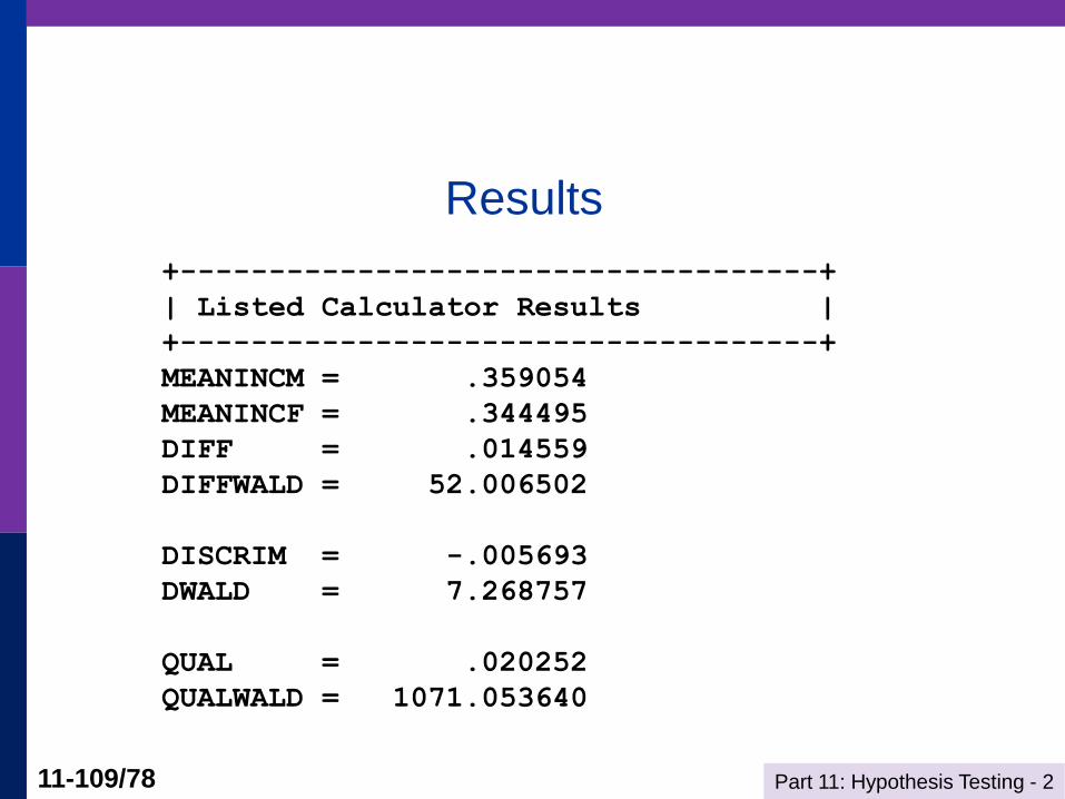
Results
+------------------------------------+
| Listed Calculator Results |
+------------------------------------+
MEANINCM = .359054
MEANINCF = .344495
DIFF = .014559
DIFFWALD = 52.006502
DISCRIM = -.005693
DWALD = 7.268757
QUAL = .020252
QUALWALD = 1071.053640
Part 11: Hypothesis Testing - 2 11-110/78
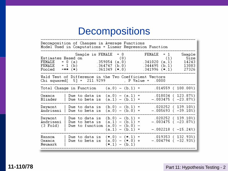
Decompositions
Part 11: Hypothesis Testing - 2 11-111/78
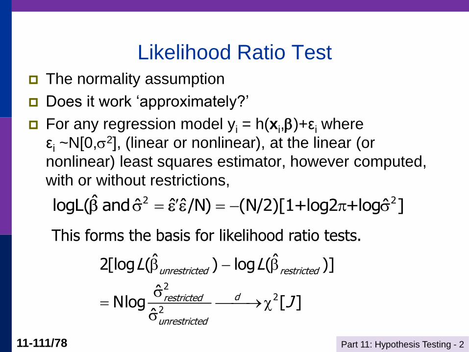
Likelihood Ratio Test
The normality assumption
Does it work ‘approximately?’
For any regression model yi = h(xi,)+εi where
εi ~N[0,2], (linear or nonlinear), at the linear (or
nonlinear) least squares estimator, however computed,
with or without restrictions,
2 2ˆlogL( and /N) (N/2)[1+log2 +log ]ˆˆˆ ˆ
This forms the basis for likelihood ratio tests.
22
2
ˆ ˆ2[log ( ) log ( )]
ˆNlog [ ]
ˆ
unrestricted restricted
drestricted
unrestricted
L L
J
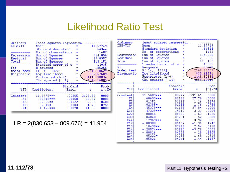
Part 11: Hypothesis Testing - 2 11-112/78
LR = 2(830.653 – 809.676) = 41.954
Likelihood Ratio Test