ECON205 Intermediate Mathematics for Economics

Lecture Notes Chapter 1. Introduction and Basics

I. ECONOMIC MODELS

1. What is a mathematical model?

What is a mathematical model? It is a set of equations used to describe or explain certain aspects of the world.

For example, we can hypothesize the following (simplified) model to predict a country's GDP:

𝑌 𝑎 𝑏𝐸 𝑐𝐿 𝑑𝑇 𝑒𝑊 𝑓𝐻

in which, 𝐸 , 𝐿 , 𝑇 , 𝑊 , and 𝐻 are the predictive variables, and 𝑎 , 𝑏 ,…are the parameters to be determined (through various econometric methods). A question: should we use consumption to be one of the factors to predict GDP? Why or why not?

2. Economic models

An example of a simple economic model: the AD-AS model. Aggregate demand is given as

𝑌 𝑎 𝑏𝑃

While Aggregate Supply is

𝑌 𝑐 𝑑𝑃

Together they form a model that describes how output and prices are determined.

2.1. Ingredients of an economic model

What does an economic model need? It needs first of all economic variables, unknown economic quantities that we seek to explain in a model, such as consumption, output, inflation…In the AD-AS model, we have two variables we seek to solve (explain), output and price level.

The model also needs parameters, numbers that are taken as given in order for the model to be solved. In the AD-AS model, the parameters are 𝑎, 𝑏, 𝑐, 𝑑.

What counts as variables or parameters depends very much on the decision of the modelers, what he/she decides are quantities that need explaining, and which quantities are taken as given.

II. SET THEORY

1. What is a set?

A set is simply a collection of objects of some common property. For example, all students studying the economics program in the School of Economics is a set. All kitchen sinks that have been bought from IKEA can also form a set. There really isn't a limit to what constitutes a set, provided we can identify at least one common property that is characteristic of all members in that set.

We use the following ways to express sets:

- enumeration: 𝑋 𝑟𝑒𝑑, 𝑔𝑟𝑒𝑒𝑛, 𝑏𝑙𝑢𝑒

- definition: 𝑋 𝑥, 𝑥: 𝑝𝑟𝑖𝑚𝑎𝑟𝑦 𝑐𝑜𝑙𝑜𝑟𝑠 𝑖𝑛 𝑡ℎ𝑒 𝑅𝐺𝐵 𝑐𝑜𝑙𝑜𝑟 𝑠𝑐ℎ𝑒𝑚𝑒

1.1. Set membership

A set contains members. You are a member of the set of students in the School of Economics. We use the following notation to express membership

𝑥 ∈ 𝑋, 𝑤ℎ𝑒𝑟𝑒 𝑋 𝑖𝑠 𝑎 𝑠𝑒𝑡.

Obviously,

𝑀𝑖𝑐𝑘𝑒𝑦 𝑀𝑜𝑢𝑠𝑒 ∈ 𝑊𝑎𝑙𝑡 𝐷𝑖𝑠𝑛𝑒𝑦 𝑐𝑎𝑟𝑡𝑜𝑜𝑛 𝑐ℎ𝑎𝑟𝑎𝑐𝑡𝑒𝑟𝑠

1.2. Subsets and supersets

Students of ECON205 are obviously al SMU students, and the set of ECON205 students is obviously smaller than the set of all SMU students. We can say that the set of ECON205 students is a (proper) subset of the set of SMU students. Conversely, the set of SMU students is the superset of the set of ECON205 students.

Mathematically,

𝐴 ⊂ 𝐵 ⇔ 𝑖𝑓 𝑎 ∈ 𝐴, 𝑡ℎ𝑒𝑛 𝑎 ∈ 𝐵, 𝑎𝑛𝑑 𝑠𝑖𝑧𝑒 𝑜𝑓 𝐴 𝑠𝑖𝑧𝑒 𝑜𝑓 𝐵

𝐴 ⊆ 𝐵 𝑎𝑛𝑑 𝐵 ⊆ 𝐴 ⇔ 𝐴 𝐵

1.3. Null and Universal sets

The null set is a set that has no member, and it’s denoted as ∅.

On the other hand, a universal set, denoted Ω, is the set that comprises all possible members as defined by the question.

2. What can we do with sets?

2.1. Set operations

We can illustrate set operations with examples. Given

𝐴 1,2,3,4,5

𝐵 3,4,5,6,7

We can form the following sets from 𝐴 and 𝐵:

𝐶 𝑥|𝑥 ∈ 𝐴 𝑜𝑟 𝑥 ∈ 𝐵 1,2,3,4,5,6,7

𝐶 is called the union of 𝐴 and 𝐵 and is written as 𝐶 𝐴 ∪ 𝐵.

𝐷 𝑥|𝑥 ∈ 𝐴 𝑎𝑛𝑑 𝑥 ∈ 𝐵 3,4,5

𝐷 is called the intersection of 𝐴 and 𝐵 and is written as 𝐷 𝐴 ∩ 𝐵.

Note: if the sets under consideration have no common members, meaning their intersection is a null set, they are called disjoint sets. We write 𝐴 ∩ 𝐵 ∅.

𝐸 𝑥|𝑥 ∈ 𝐴 𝑎𝑛𝑑 𝑥 ∉ 𝐵 1,2

𝐸 is called the subtraction of 𝐴 from 𝐵 and is written as 𝐸 𝐴\𝐵.

If we have the following, 𝐹 Ω\𝐴, where Ω is called the universal set, 𝐹 is called the complement of 𝐴, and we can write 𝐹 �̅�.

2.2. Venn's diagrams

Set operations are best visualized with the help of Venn's diagrams. Let's have an illustration: 𝐴 ∩ 𝐵.

3. Laws on set operations

3.1. Commutation

Union and Intersection are commutative:

𝐴 ∩ 𝐵 𝐵 ∩ 𝐴 𝑎𝑛𝑑 𝐴 ∪ 𝐵 𝐵 ∪ 𝐴

3.2. Association

Union and Intersection are associative:

𝐴 ∩ 𝐵 ∩ 𝐶 𝐴 ∩ 𝐵 ∩ 𝐶

𝐴 ∪ 𝐵 ∪ 𝐶 𝐴 ∪ 𝐵 ∪ 𝐶

3.3. Distribution

Distributive laws

𝐴 ∩ 𝐵 ∪ 𝐶 𝐴 ∩ 𝐵 ∪ 𝐴 ∩ 𝐶

𝐴 ∪ 𝐵 ∩ 𝐶 𝐴 ∪ 𝐵 ∩ 𝐴 ∪ 𝐶

3.4. Complements

𝐴 ∩ 𝐵 �̅� ∪ 𝐵

𝐴 ∪ 𝐵 �̅� ∩ 𝐵

Exercises: prove the above laws using Venn's diagrams.

III. FUNCTIONS

1. What is a function

1.1. Definition

A function describes a relationship between two quantities (variables). For example, the bus fare depends on the distance travelled on the bus, thus the bus fare is a function of the travel distance. We usually call the bus fare the dependent variable, and the distance travelled the independent variables. What kind of relationship? It depends on how it is defined. For example, there is some formula used by the public transport company to calculate fare based on distance.

The most important property of functions is that, continuing with the bus fare example, different travel distances can yield the same fare, but the same travel distance cannot yield two or more different fares.

Basic definition of functions_____________________________________________________________

A (real-valued) function of a real variable x with domain D is a rule that assigns a unique real number to each real number x in D. As x varies over the whole domain, the set of all possible resulting values f (x) is called the range of f.

f: D R

1.2. Domain and range of a function

Let's look at the function 𝑓 𝑥 √𝑥. Obviously, 𝑓 doesn't take values of 𝑥 that are 0. The set of 𝑥 that make 𝑓 defined is called the domain of 𝑓.

Example: find the domain of the following functions

a. 𝑓 𝑥

b. 𝑔 𝑧 √2𝑥 5

Again, let's look at 𝑓 𝑥 √𝑥. If we use all the values of 𝑥 in the domain of 𝑓 to compute 𝑓 𝑥 , we will find that 𝑓 𝑥 can take all values 0. The set of all possible values of 𝑓 𝑥 is called the range of 𝑓.

Example: the cost of producing x units of a commodity is given by 𝐶 𝑥 1000 300𝑥 𝑥 .

(a) Compute 𝐶 0 . What does it mean?

b. Compute 𝐶 𝑥 /𝑥. What does it mean?

(b) Compute 𝐶 𝑥 1 𝐶 𝑥 , and explain in words the meaning of the difference.

2. Graph of a function

Review textbook section 4.3.

3. Different types of functions

3.1. Linear functions

Linear functions have a simple form

𝑓 𝑥 𝑎𝑥 𝑏

which is a straight line if drawn using the x-y coordinates.

Many economic relationships are assumed to be linear. For example, demand functions

𝐷 𝑃 𝑎 𝑏𝑃

and supply functions

𝑆 𝑃 𝑐 𝑑𝑃

3.2. Quadratic functions

𝑓 𝑥 𝑎𝑥 𝑏𝑥 𝑐

3.3. Polynomials

𝑓 𝑥 𝑎 𝑥 𝑎 𝑥 ⋯ 𝑎

3.4. Power functions

𝑓 𝑥 𝑎𝑥

3.5. Exponential and logarithmic functions

𝑓 𝑥 𝑎𝑒

𝑓 𝑥 𝑙𝑛𝑥

4. Changing function

4.1. Composite function

Given 𝑓 𝑥 and 𝑔 𝑥 , we have

𝑓 ∘ 𝑔 𝑥 𝑓 𝑔 𝑥

Example: given 𝑓 𝑥 2𝑥 and 𝑔 𝑥 √𝑥, we have 𝑓 ∘ 𝑔 𝑥 𝑓 𝑔 𝑥 𝑓 √𝑥 2√𝑥.

4.2. Inverse function

Consider the demand function

𝐷30

𝑃 /

A producer would care about the price that would result if he/she sets production (output) at a certain level. Thus what he/she would want to know is the inverse relationship.

𝑃30𝐷

In general, given 𝑦 𝑓 𝑥 , we have

𝑥 𝑓 𝑦

This 𝑓 is the inverse of 𝑓. Conditions for a function to have an inverse:

___________________________________________________________________________________

A (real-valued) function of a real variable f(x) has an inverse if and only if it is a one-to-one function.

Example: find the inverse functions of the following functions

(a) 𝑦 4𝑥 3

(b) 𝑦 √𝑥 1

(c) 𝑦

IV. EQUATIONS

1. What is an equation

Earlier, when we learn about functions, we compute a value of a function, say 𝑓 𝑥 , by putting a value of 𝑥 into 𝑓 𝑥 . When we want to do the reverse, finding 𝑥 given a value of 𝑓 𝑥 , we set up the following

𝑓 𝑥 𝑎

What we have is an equation.

For example, given 𝑓 𝑥 𝑥 , find 𝑥 so that 𝑓 𝑥 4. We have the following equation

𝑥 4

Almost any equation can be thought of this way.

2. Rules concerning equations

The following things can be done with equations to help you solve them

If 𝐴 𝐵

- 𝐴 𝑎 𝐵 𝑎

- 𝐴/𝑎 𝐵/𝑎, only if 𝑎 0.

- 𝐴𝑎 𝐵𝑎, again only if 𝑎 0.

𝐴, 𝐵, 𝑎 stand for numbers, constants, functions, variables…

3. Solving equations

Review textbook chapter 3.

V. GEOMETRIC SERIES

Let 𝑎, 𝑎𝑘, 𝑎𝑘 , 𝑎𝑘 , … , 𝑎𝑘 be a finite geometric series.

The sum of finite geometric series is given by

𝑆 𝑎 𝑎𝑘 𝑎𝑘 ⋯ 𝑎𝑘

𝑎 1 𝑘

1 𝑘 𝑘 1

Theorem: Let 𝑎, 𝑎𝑘, 𝑎𝑘 , 𝑎𝑘 , … , 𝑎𝑘 , … be an infinite geometric series. Then if |𝑘| 1, we can find:

𝑎 𝑎𝑘 𝑎𝑘 ⋯ 𝑎𝑘 ⋯ 𝑎

1 𝑘

ECON205 Intermediate Mathematics for Economics

Lecture Notes Chapter 2. Equilibrium Analysis (Textbook Chapters 15, 16)

I. EQUILIBRIUM ANALYSIS

1. Economic equilibria

Economics is all about equilibrium: equilibrium in a game, equilibrium in a market. Almost all economic analyses are made with an equilibrium as starting point. Put in simple language, when a system or a model reaches an equilibrium, there’s no tendency for variables within the system/model to change. This is why equilibrium analysis is also called static analysis (as opposed to dynamic analysis that we will learn in chapter 5)

Not all equilibria are desirable. Some are naturally desirable, such as the market outcome of an ideal economy, while some are not (such as in an economy with public good or externality). In the topics of optimization, we will learn how to arrive at goal equilibria, i.e. desirable equilibria that result from our conscious decision to make them so.

We start by looking at the most basic but also the most fundamental equilibrium in economics: the one-market partial equilibrium model

2. A simple partial equilibrium model

Let's consider the market for apple. The demand law says that the quantity demanded of apples is related to its price by the following

𝑄 𝑎 𝑏𝑃

The law of supply says that the quantity of apples supplied is related to the price of apples by the following

𝑄 𝑐 𝑑𝑃

We have three variables, but only two equations. We need one more condition to make the model complete. Since the model is about the equilibrium in the market for apple, we invoke the equilibrium condition

𝑄 𝑄

Now the model is complete. The equilibrium in the market for apples is given by the above three equations, and they can be solved for us to obtain the equilibrium price and equilibrium quantity. What do they mean, equilibrium price and quantity? It means that when the actual price of apples is equal to the equilibrium price, the quantity demanded is equal to the quantity supplied equal to the equilibrium quantity, and neither the price nor quantity has any tendency to move.

Why is this equilibrium called a partial equilibrium? This is because we are considering the market for apples in isolation, and we assume that everything else remains constant, so that nothing outside the apple market affects it and whatever happens in the market for apples does not affect anything outside it, either. Partial equilibrium is useful, but it is incomplete, because no market for any goods is in isolation, and so equilibrium in the market for one good tends to affect the equilibrium in the market for another good. In order to have a more complete picture of the equilibria of multiple markets and how they interact with one another, we need to consider the concept of general equilibrium.

2. General equilibrium

General equilibrium is the situation in which several connected markets are in equilibrium simultaneously. This is not the case of simply putting several sets of equations of the above model (one set for one market) together. Why is that? If you are familiar with the concept of cross-price elasticity, you can answer this question. The simple answer is that what happens to the equilibrium price of one good affects the demand and supply of another good.

This means that in a general equilibrium, the demand and supply for one good need to be modified to include the price effects of all the other goods. We can start with a general equilibrium for a two-good market model.

𝑄 𝑎 𝑏𝑃 𝛼𝑃

𝑄 𝑐 𝑑𝑃 𝛽𝑃

𝑄 𝑒 𝑓𝑃 𝛾𝑃

𝑄 𝑔 ℎ𝑃 𝜀𝑃

𝑄 𝑄

𝑄 𝑄

As you can expect, for a market of 𝑛 goods, the set of questions describing its general equilibrium gets large (2𝑛 equations with 2𝑛 variables large), and solving this set of questions by substitution or elimination methods is just not feasible.

Finding an economic equilibrium involves finding a solution to a system of equations, which can be large and complex, so questions naturally arise:

- How do we know if such a system gives us a solution in the first place?

- And if it does, how do we find this solution?

To answers these questions, we need to bring in matrix algebra, the mathematical tools using matrices.

II. MATRIX ALGEBRA

1. What are matrices and vectors?

Matrices are mathematical objects of two dimensions, meaning each has rows and columns, and at each intersection of a row and a column is an entry (or element) that contains (usually) a number.

A typical matrix

3 4 5

172

0.7

This matrix has two row and three columns, containing six elements. We call this a 2 3 matrix (number of rows number of columns). For matrix algebra, we stick to elements that are real numbers (matrix algebra with complex numbers as elements is called linear algebra.)

Thus, in general, an 𝑚 𝑛 matrix has the following form

𝑎 ⋯ 𝑎⋮ 𝑎 ⋮

𝑎 ⋯ 𝑎

An element 𝑎 in the matrix helps us identify its position: 𝑖 refers to its row, 𝑗 its column.

Vectors are simply a special type of matrices, with just one row or one column. Matrices with just one row are called row vectors; matrices with one column are called column vectors.

Examples:

1 1 1 , 4 √3 1.523

, 0 5

22

,9

3419

2. Matrix operations

What can we do with matrices and vectors? It is usually to think of them as a very general type of numbers. We can add, subtract and multiply them, even though the rules are more restrictive.

2.1. Matrix addition and subtraction

Matrices and vectors can be added and subtracted just as numbers can, with one catch: the matrices or vectors in addition or subtraction must be of the same dimensions.

𝐴 𝐵 𝑎 𝑏 𝑎 𝑏

2.2. Matrix multiplication

2.2.1. Scalar multiplication

Scalar multiplication is multiplication of a matrix by a number. It is straightforward:

𝛽𝑎 ⋯ 𝑎

⋮ 𝑎 ⋮𝑎 ⋯ 𝑎

𝛽𝑎 ⋯ 𝛽𝑎⋮ 𝛽𝑎 ⋮

𝛽𝑎 ⋯ 𝛽𝑎

2.2.2. Matrix multiplication

Multiplying matrices together is a lot trickier, because it has to follow a very strict rule. The rule is, 𝐴 𝐵, or just 𝐴𝐵, is only possible if the number of columns of A is equal to the number of rows of B.

Obviously, if neither 𝐴 or 𝐵 is square, and 𝐴𝐵 is possible, then 𝐵𝐴 is not.

Let’s learn the technique of matrix multiplication through an example (further reading textbook section 15.3.)

Example: Suppose that

𝐴 1 0 32 1 5

and 𝐵 1 32 56 2

. Then we define AB

𝐴𝐵 1 0 32 1 5

1 32 56 2

1 . 1 0 . 2 3 . 6 1 . 3 0 . 5 3 . 22 . 1 1 . 2 5 . 6 2 . 3 1 . 5 5 . 2

19 934 21

2.2.3. First step in solving a system of linear equations - rewriting a system of equation in matrix form

With matrix multiplication, we can now use matrix algebra for one of its most useful purpose. Let's recall the system of equations describing the general equilibrium in the n-commodity market.

𝑎 𝑃 𝑎 𝑃 ⋯ 𝑎 𝑃 𝑑

𝑎 𝑃 𝑎 𝑃 ⋯ 𝑎 𝑃 𝑑

⋮

𝑎 𝑃 𝑎 𝑃 ⋯ 𝑎 𝑃 𝑑

This system can be neatly rewritten in matrix form as

𝐴𝑥 𝑑

where

𝑥𝑃⋮

𝑃, 𝐴

𝑎 ⋯ 𝑎⋮ ⋱ ⋮

𝑎 ⋯ 𝑎, 𝑑

𝑑⋮

𝑑

2.3. Matrix division

There is only one kind of matrix division allowed: division by a scalar. In this regard, division by a scalar is just multiplication by the reciprocal of that scalar. In other words, there is simply no division of matrix.

2.4. Laws on matrix operations

The laws on number operations are easily understood: addition is both associative and commutative, while subtraction is not, and so on. Matrices follow similar rules.

Matrix addition is both associative and commutative, that is,

𝐴 𝐵 𝐶 𝐴 𝐵 𝐶 𝑎𝑛𝑑 𝐴 𝐵 𝐵 𝐴

Matrix subtraction is not strictly associative and commutative, but with a bit of modification it is

𝐴 𝐵 𝐶 𝐴 𝐵 𝐶 𝑎𝑛𝑑 𝐴 𝐵 𝐵 𝐴

Scalar multiplication is distributive over addition and subtraction:

𝛼 𝛽 𝐴 𝛼𝐴 𝛽𝐴

𝛼 𝐴 𝐵 𝛼𝐴 𝛼𝐵

Matrix multiplication is distributive over addition and subtraction:

𝐴 𝐵 𝐶 𝐴𝐵 𝐴𝐶

𝐵 𝐶 𝐴 𝐵𝐴 𝐶𝐴

Matrix multiplication is also associative:

𝐴 𝐵𝐶 𝐴𝐵 𝐶

Importantly, matrix multiplication is not commutative, that is,

𝐴𝐵 𝐵𝐴

This means that the distributive rules for matrix multiplication have to follow the exact order in which the matrices are multiplied.

2.5. Null and identity matrices

A null matrix is the equivalent of zero in matrix algebra. It has all elements equal to zero, and it serves the purpose:

𝐴 𝐴 𝟎

An identity matrix is a square matrix, with 1's on its diagonal entries, and zero's on all its other entries.

Example, a 3 3 identity matrix,

1 0 00 1 00 0 1

Identity matrices are like the number 1. Their beauty is shown by, for any square matrix and the identity matrix of the same dimensions:

𝐴 𝐼𝐴 𝐴𝐼

Identity matrices are important for the concept of matrix inverses.

2.6. Transposes and inverses

2.6.1. Transposes

A transpose of a matrix is obtained when the columns of that matrix become rows, so that its rows become columns.

The transpose of

1 29 0

√2 6

is

1 9 √22 0 6

2.6.2. Laws on transposes

a. 𝐴 𝐴

b. 𝐴 𝐵 𝐴 𝐵′

c. 𝛼𝐴 𝛼𝐴′

d. 𝐴𝐵 𝐵′𝐴′

Note: A square matrix A is symmetric if 𝑨 𝑨

2.6.3. Inverses

An inverse is like a reciprocal of a matrix. However, this is exclusively the domain of square matrices (matrices that have equal numbers of rows and columns). Remember: talk of inverses is irrelevant for non-square matrices.

The inverse of a square matrix 𝐴 is 𝐴 , and it works this way

𝐴𝐴 𝐼

where 𝐼 is an identity matrix of the same dimensions as 𝐴. And conversely, 𝐴 is the inverse of 𝐴 .

Not all square matrices have inverses. Square matrices that have inverses are called invertible or non-singular. Square matrices that do not have inverses are called singular matrices. And of course, the inverse of a square matrix (if it has one) is unique.

2.6.4. Laws on inverses

Let A and B be invertible n × n matrices. Then:

a. 𝑨 𝟏 is invertible, and 𝑨 𝟏 𝟏 𝑨.

b. 𝑨𝑩 is invertible, and 𝑨𝑩 𝟏 𝑩 𝟏𝑨 𝟏.

c. The transpose of 𝑨 is invertible, and 𝑨 𝟏 𝑨 𝟏 ′.

d. 𝑐𝑨 𝟏= 𝑐 𝑨 𝟏 whenever 𝑐 is a number 0.

(Textbook theorem 16.6.1)

2.6.4. Second step in solving a system of linear equations

Knowing what we know about inverse, from

𝐴𝑥 𝑑

We get

𝐴 𝐴𝑥 𝐴 𝑑 ⟹ 𝑥 𝐴 𝑑

What is left is simple matrix multiplication, and we can solve for 𝑥. But of course the problem now is whether there is even 𝐴 , because not every square matrix is invertible (non-singular).

There are now two things to do before we can arrive at a solution for a system of linear equations:

- Check whether 𝐴 exists (whether 𝐴 is non-singular)

- Compute 𝐴

We will tackle the first task by learning more about vectors.

2.7. More on vectors

We need to look more closely at vectors, because they are relevant to the issue of matrix non-singularity.

Consider the following matrix

4 7 15 0 2

From it we can pick out these vectors 45

, 70

, 12

. Obviously, these form the columns of the matrix. Thus,

these vectors are called column vectors of this matrix. Likewise, the row vectors of this matrix are 4 7 1 , 5 0 2 .

Thus, given any matrix 𝐴 of dimensions 𝑚 𝑛, it contains 𝑚 row vectors of dimensions 1 𝑛 and 𝑛 column vectors of dimensions 𝑚 1.

But what is so special about the rows and columns of a matrix? The question of linear independence.

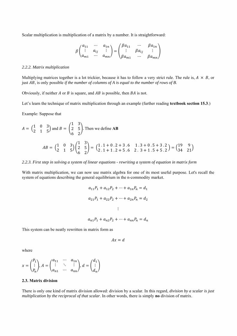
2.7.1. Linear independence

Question: Given the below three vectors, what can you observe about them?

45

, 70

, 22

Answer: one can be expressed as a linear combination of the other two, in this way

45

97

70

52

22

Question: What about this group of vectors?

100

,01

0,

002

Answer: none of them is a linear combination of any of the others in the group.

The first group of vectors is said to be linearly dependent, while the second group is linearly independent.

Note: The concept of linear independence applies to both row and column vectors.

A useful result on linear independence ____________________________________________________

In the space containing all vectors of dimensions 𝑛 1 or 1 𝑛, any group of 1 𝑛 vectors is linearly dependent.

Applying the concept of linear independence to the row or column vectors of a matrix, we can ask whether they are linearly independent. How do we do that? One method is by visual inspection, but this method's usefulness runs out fast when we look at a large number of vectors, when it is no longer easy to spot any patterns among them. The second method is by using what we call elementary row operations.

2.7.2. Elementary row operations

The purpose of this operation is to reduce any matrix to its echelon form. We will be doing this in details in class, and for further review, please refer to the full exposition of this in textbook section 15.6.

3. Solving systems of linear equations

What is so special about the concept of linear independence among the row or column vectors of a matrix? When we apply it to a square matrix, we can answer the question whether that matrix is non-singular.

Recall a system of equations in matrix form

𝐴𝑥 𝑑

where 𝐴 is the square coefficient matrix, 𝑥 is the vector of variables that we need to solve, and 𝑑 is a vector of constants. 𝑥 is found by

𝑥 𝐴 𝑑

Whether we can find values for 𝑥 depends on 𝐴, specifically whether it has an inverse. Non-singularity of 𝐴 permits its inverse, and inverses are all that matter to the solution of a system of linear equations.

And it turns out that we can check whether 𝐴 is non-singular by checking for the linear independence among the row vectors of 𝐴. The link is simple:

A square matrix is non-singular all of its rows or columns are linearly independent.

So the first simple condition to check whether a square matrix has an inverse is to check whether all of its rows or columns are linearly independent. And we have learned the method of elementary row operations, which can be used to deduce whether all the row or column vectors in a matrix are linearly independence.

Example: given,

1 2 11 1 11 7 5

After applying the elementary row operations, we obtain the echelon form

1 2 10 3 20 0 0

It is straight-forward to see that the non-zero rows in the echelon form are linearly independent with one another (zero vectors are never linearly independent). What can we conclude? Only two of the original matrix's vectors are linearly independent, because one of its rows has been reduced to zero, so, this matrix does not have all linearly independent row or column vectors. We can conclude further that since not all of its rows are linearly independent, this matrix is singular.

Example of a non-singular matrix:

1 1 30 2 13 2 2

and its echelon form

1 1 30 2 10 0 27/2

As we can see from the echelon form of this matrix, all of its rows remain non-zero, meaning that all three of its rows are linearly independent with one another. Thus, this matrix is non-singular.

3.1. Rank

The rank of a matrix is defined as the maximum number of its row or column vectors that are linearly independent. Row vectors or column vectors? It turns out it doesn't matter: the number of independent row vectors is the same as the number of independent column vectors for every matrix.

3.1.1. Finding the rank of a matrix

We have learned this method; it is nothing other than reducing the rows of a matrix down to its echelon form. The number of non-zero row vectors that remain is the rank of the matrix.

3.1.2. Full-rank matrix

A matrix that has a rank equal to its number of rows or columns (whichever is smaller), is called a full-rank matrix.

3.1.3. Rank and non-singularity

So now it is time to link the rank of a square matrix to whether it is non-singular. The link is simple:

A square matrix is non-singular it is a full-rank matrix.

Putting everything that we have so far

A square matrix is non-singular all of its rows or columns are linearly independent it is a full-rank matrix.

3.2. Determinant

Every square matrix has a determinant associated with it (like its identification number). A determinant of a square matrix is a number.

3.2.1. Calculating determinant

A determinant of a 2 2 matrix

𝐴 𝑎 𝑏𝑐 𝑑

is

|𝐴| 𝑎𝑑 𝑏𝑐

How about a 3 3 matrix? We find its determinant by iteration. Starting with

𝐵𝑎 𝑏 𝑐𝑑 𝑒 𝑓𝑔 ℎ 𝑖

The determinant of B is

|𝐵| 𝑎 𝑒 𝑓ℎ 𝑖

𝑏𝑑 𝑓𝑔 𝑖 𝑐

𝑑 𝑒𝑔 ℎ 𝑎 𝑒𝑖 ℎ𝑓 𝑏 𝑑𝑖 𝑔𝑓 𝑐 𝑑ℎ 𝑔𝑒

See the pattern there?

Please review textbook sections 16.1, 16.2, 16.3 regarding cofactors and how to derive them.

For matrices of greater dimensions, we can keep iterating, but of course it gets very long, and so calculating the determinant of a large matrix is usually the task of a computer.

3.2.2. Determinant and rank and linear independence

What is a determinant for? First, it provides a faster way (now with computers) to check for linear independence among the rows or columns of a square matrix. The link between the determinant of a square matrix and linear independence of its row (column) vectors is clear: if the determinant of the matrix is non-zero, the matrix is full-rank, that is, all of its row (column) vectors are linearly independent.

Thus, there are now two ways of checking for linear independence among the rows or columns of a matrix. One is by elementary row operations; the other is by calculating its determinant.

Second, determinant is indispensable in the calculation of inverses (later).

3.2.3. Determinant and non-singularity

Knowing what we know about non-singularity of a matrix and its rank, we then can see that a determinant of a matrix tells us whether it is non-singular or not as well. We now have the full result.

Putting everything together____________________________________________________________

A square matrix is non-singular all of its rows or columns are linearly independent it is a full-rank matrix the determinant of the matrix is non-zero.

3.2.4. Properties of determinants

For any 𝑛 𝑛 A matrix,

A. If all the elements in a row (or column) of A are 0, then |A| = 0. A direct corollary of this is if two of the rows (or columns) of A are proportional, then |A| = 0. B. |A'| = |A|, where A' is the transpose of A. C. If all the elements in a single row (or column) of A are multiplied by a number α, the determinant is multiplied by α. A corollary of this is that, if α is a real number, |αA| = αn|A| D. If two rows (or two columns) of A are interchanged, the determinant changes sign, but the absolute value remains unchanged. E. The value of the determinant of A is unchanged if a multiple of one row (or one column) is added to a different row (or column) of A. F. The determinant of the product of two 𝑛 𝑛 matrices A and B is the product of the determinants of each of the factors:|AB| = |A| ꞏ |B|.

3.3. Finding inverses

3.3.1. With elementary row operations

We will be doing this in details in class, and for further review, please refer to the full exposition of this in textbook section 16.7.

3.3.2. With determinant

Textbook section 16.7, theorem 16.7.1.

3.4. Solving systems of linear equations with inverses

So, after we learn about the methods of checking whether a square matrix is non-singular as well as methods of calculating inverses, we can get to the main business of solving a system of linear equations.

General result for the solutions to a system of linear equations__________________________________

Given

𝐴𝑥 𝑑

1. If |𝐴| 0, the system has a unique solution vector 𝑥, and 𝑥 𝐴 𝑑.

2. If |𝐴| 0, the system either has no solution or an infinite number of solutions.

Example: consider the following system

𝑎𝑥 𝑏𝑦 𝛼

𝑐𝑥 𝑑𝑦 𝛽

where 𝑥 and 𝑦 are variables to be found. The system in matrix form is

𝑨𝒛 𝒅

where

𝑨 𝑎 𝑏𝑐 𝑑

, 𝒛𝑥𝑦 , 𝒅

𝛼𝛽

The determinant of 𝐴 is

|𝑨| 𝑎𝑑 𝑏𝑐

If 𝑎𝑑 𝑏𝑐, |𝐴| 0, the system has a unique solution, and it is given by

𝒛𝑥𝑦 𝑨 𝟏𝒅

1𝑎𝑑 𝑏𝑐

𝑑 𝑏𝑐 𝑎

𝛼𝛽

Graphically, this is the case of two lines in a plane that intersects at one point.

If 𝑎𝑑 𝑏𝑐, |𝑨| 0. And if, further,

𝛼𝛽

𝑎𝑐

𝑏𝑑

the two equations are actually just one equation, and the system gives an infinite number of solutions, that is, there are infinitely many 𝑥 and 𝑦 that satisfy the system. Graphically, this is the case of the two lines coinciding in a plane.

But if

𝛼𝛽

𝑎𝑐

𝑏𝑑

then we have no solutions. No 𝑥 and 𝑦 exist to satisfy the system. This is the equivalent of two parallel lines.

3.5. Cramer's Rule

Cramer's Rule is very useful for finding the solution to a system of two linear equations, and is straightforward to apply. We will discuss this in class with hands-on examples. Please refer to textbook section 16.8 for review.

III. FURTHER APPLICATIONS

1. IS-LM model

A simple model of the macroeconomy involves two markets: goods market and money market.

The goods market has the following equations

𝑌 𝐶 𝐼 �̅�

𝐶 𝑎 𝑏 1 𝑡 𝑌

𝐼 𝑑 𝑒𝑖

The money market

𝑀 𝑀

𝑀 𝑘𝑌 𝑙𝑖

Putting everything together, we have four equations with four variables 𝑌, 𝐶, 𝐼 and 𝑖:

𝑌 𝐶 𝐼 �̅�

𝐶 𝑎 𝑏 1 𝑡 𝑌

𝐼 𝑑 𝑒𝑖

𝑀 𝑘𝑌 𝑙𝑖

Putting this system in matrix form:

1𝑏 1 𝑡

0𝑘

11

00

1010

00𝑒

𝑙

𝑌𝐶𝐼𝑖

�̅�𝑎

𝑑𝑀

2. The Leontief input-output model

Once upon a time, in an ancient land perhaps not too far from Norway, an economy consisted of three industries—fishing, bread baking, and forestry.

To produce 1 ton of fish requires 𝑎 tons of fish, 𝑎 tons of timber and 𝑎 tons of bread.

To produce 1 ton of timber requires 𝑏 tons of fish, 𝑏 tons of timber and 𝑏 tons of bread.

To produce 1 ton of bread requires 𝑐 tons of fish, 𝑐 tons of timber and 𝑐 tons of bread.

These are the only inputs needed for each of these three industries. Find what gross outputs each of the three industries must produce in order to also meet the demands of 𝑑 tons of fish, 𝑑 tons of timber and 𝑑 tons of bread for the general population.

ECON205 Intermediate Mathematics for Economics

Lecture Notes Chapter 3. Comparative Statics

I. THE CONCEPT OF COMPARATIVE STATICS

Let's go back to the competitive equilibrium of a market of a commodity

𝑄 𝑎 𝑏𝑃

𝑄 𝑐 𝑑𝑃

𝑄 𝑄

Solving for equilibrium price and quantity we obtain

𝑃∗ 𝑎 𝑐𝑏 𝑑

𝑄∗ 𝑎 𝑏𝑎 𝑐𝑏 𝑑

𝑎𝑑 𝑏𝑐𝑏 𝑑

Now, we may have questions such as: what happens to the equilibrium price and quantity when the demand is more elastic, that is, when 𝑏 is larger in magnitude? It may be possible to find out just by visual checking in this case, but we need a more general way that will work for much more complicated systems.

This is where we need to rely on derivatives to help us find the answers to this type of questions.

II. DERIVATIVES

1. What is a derivative of a function?

A derivative of a function, at the core, is the rate of change of the function when its independent variable changes.

1.1. Rate of change

Given a function

𝑦 𝑓 𝑥

At 𝑥 𝑥 , the function takes the value 𝑦 𝑓 𝑥 . As 𝑥 changes to 𝑥 , the function value becomes 𝑦 𝑓 𝑥 . We can look at how much the function changes per unit change in 𝑥 by the following formula:

∆𝑦∆𝑥

∆𝑓∆𝑥

𝑓 𝑥 𝑓 𝑥𝑥 𝑥

This is called the rate of change of 𝑓. Obviously the rate of change depends on the functional form of 𝑓, as well as the two values 𝑥 and 𝑥 . If 𝑥 𝑥 ℎ, we have

𝑓 𝑥 𝑓 𝑥𝑥 𝑥

𝑓 𝑥 ℎ 𝑓 𝑥ℎ

Now we focus on the change interval ℎ. If we take ℎ to be smaller and smaller, we arrive at the instantaneous rate of change of 𝑓 at 𝑥 :

𝒅𝒚𝒅𝒙

𝑑𝑓𝑑𝑥

𝑓 𝑥 ℎ 𝑓 𝑥ℎ

𝑎𝑠 ℎ → 0

This is called the first-order derivative of 𝒇 with respect to 𝒙 at 𝒙𝟏.

1.2. Derivatives and slopes

The derivative of a function 𝑓 𝑥 at any point 𝑥 is simply the slope (gradient) of the function at that point.

How do we find the derivative of a function? We need to take a detour and learn about limits first.

2. Limits

2.1. What is a limit?

Take the function 𝑓 𝑥 2𝑥. At 𝑥 2, 𝑓 𝑥 𝑓 2 4. If we take 𝑥 1 and make 𝑥 approach 2, 𝑓 𝑥 approaches 𝑓 2 . We say in this case that 𝑓 2 is the limit of 𝑓 𝑥 when 𝑥 → 2. We write: lim

→𝑓 𝑥 𝑓 2 4.

In general, writing lim→

𝑓 𝑥 𝐴 means that we can make 𝑓 𝑥 as close to 𝐴 as we want by bringing 𝑥

as sufficiently close to (but not equal to) 𝑎 as possible.

2.1.1. Left-sided and right-sided limits

Surely the limit should be the same whether we approach a value of x from either direction? Not always. For example, consider the following examples:

a. 𝑓 𝑥1 𝑥 𝑓𝑜𝑟 𝑥 1

1 𝑓𝑜𝑟 𝑥 1

b. 𝑓 𝑥 , 𝑥 1

2.1.2. Existence of limits

Condition for the existence of limits_______________________________________________

A limit exists if and only if both of its right-side and left-side limits exist and are equal.

2.2. Rules for limits

If lim→

𝑓 𝑥 𝐴 and lim→

𝑔 𝑥 𝐵, then

a. lim→

𝑓 𝑥 𝑔 𝑥 𝐴 𝐵

b. lim→

𝑓 𝑥 𝑔 𝑥 𝐴𝐵

c. lim→

(if 𝐵 0)

d. lim→

𝑓 𝑥 𝐴 (if 𝐴 is defined and 𝑟 is any real number)

2.3. Calculating limits, L'Hôpital Rule

The easiest, most intuitive way to calculate the limit of 𝑓 𝑥 as 𝑥 → 𝑎 is to calculate 𝑓 𝑎 , right? Yes, but only sometimes. Sometimes we run into the following situations:

a. lim→

or lim→

b. lim→

∞ ∞, lim→

Examples:

a. 𝑓 𝑥 1 𝑥 / 1 𝑥 , 𝑥 → 1

b. 𝑓 𝑥 2𝑥 5 / 𝑥 1 , 𝑥 → ∞

Thus the next approach, when the simple way above doesn't work, is to reduce the function down to the extent that it then can work. Task: try with the above examples.

But sometimes, there is simply no way to reduce the function further, and in this case we need to apply L'Hôpital Rule.

L'Hôpital Rule: for the case of 𝑙𝑖𝑚 , we have

lim→

𝑓 𝑥𝑔 𝑥

lim→

𝑓 𝑥𝑔 𝑥

𝑓 𝑎𝑔 𝑎

Examples:

a. lim→

b. lim→

2.4. Applying limits

2.4.1. Continuity

A function is said to be continuous at a point on its domain if its value doesn't 'jump' too much as it traverses the point from one side to the other. This is usually taken to mean that the function doesn’t have gaps.

The condition for continuity_____________________________________________________

A function 𝑓 𝑥 is said to be continuous at 𝑥 , if and only if the limit of 𝑓 𝑥 as 𝑥 approaches 𝑥 is 𝑓 𝑥 , that is,

𝑙𝑖𝑚→

𝑓 𝑥 𝑓 𝑥

This condition may look simple, but it actually encompasses three separate conditions for continuity:

1) 𝑓 𝑥 is defined.

2) The limit 𝑙𝑖𝑚→

𝑓 𝑥 exists.

3) The limit must be equal to 𝑓 𝑥 .

2.4.2. Interest compounding

Let's use an example. You want to save $1000 for 𝑡 years, with an annual interest rate of 10%. After 𝑡 years, your $1000 will have become

𝐹𝑉 1000 1 0.1

Now imagine that the interest accumulates daily instead of yearly.

𝐹𝑉 1000 1 0.1/365

In general

𝐹𝑉 𝑆 1 𝑟/𝑛

Now imagine that the compounding is continuous, meaning that the interest accumulates constantly over infinitesimal periods of time (𝑛 → ∞).

lim→

𝑆 1 𝑟/𝑛 𝑆 𝑒

What about discounting? It is just the opposite of interest compounding

𝑃𝑉 1000 1 0.1

and so generally,

𝑃𝑉 1000 1 𝑟/𝑛

and with continuous discounting

𝑃𝑉 1000𝑒

3. Derivatives

3.1. Definition of derivatives

Using what we learned about limits, the derivative of a function 𝑦 𝑓 𝑥 is simply the limit of its rate of change, defined at a point in the domain of the function:

𝑑𝑦𝑑𝑥

𝑑𝑓 𝑥𝑑𝑥

lim→

𝑓 𝑥 ℎ 𝑓 𝑥ℎ

Here we take 𝑥 to be a general value of the independent variable, since the definition of derivative is the

same for every point in the domain of the function. We also write as 𝑓 𝑥 .

And now, with all the skills learnt to find limits, we can develop the derivatives of basic functions. The process of finding derivatives is called differentiation.

3.2. Finding derivatives using limits

The best way to learn this is through an example. Find the derivative of

𝑦 𝑓 𝑥 𝑥

Applying the limit-based definition of derivative for a general value 𝑥 in the domain of 𝑓 𝑥 :

𝑓 𝑥 lim→

𝑓 𝑥 ℎ 𝑓 𝑥ℎ

lim→

𝑥 ℎ 𝑥ℎ

lim→

𝑥 2𝑥ℎ ℎ 𝑥ℎ

lim→

2𝑥ℎ ℎℎ

lim→

2𝑥 ℎ 2𝑥

3.3. Differentiability

As is the problem with limits sometimes, the derivative may not exist at a particular point 𝑥 . Look

at the graph of a function below.

Clearly, the function is not continuous at 𝑥 , and so there can't be any defined slope at that point, thus no derivative is defined at 𝑥 . We say that the function is not differentiable there. Therefore, a function first needs to be continuous at a point before it can be differentiable.

However, continuity is only the necessary condition for differentiability, because even when a function is continuous, there is no guarantee it is differentiable, as shown below

The sufficient condition for differentiability is that the limit lim→

must be defined.

Note: In everyday language, a function is differentiable at a point when it is 'smooth' at that point.

3.4. Derivatives of basic functions and rules of differentiation

(Study textbook sections 6.6, 6.7, 6.8 and 7.3).

3.5. Derivatives of higher order

or 𝑓′ 𝑥 is the first-order derivative of 𝑓 with respect to 𝑥. 𝑓′ 𝑥 itself is a function, and if it is

differentiable, we can obviously differentiate 𝑓′ 𝑥 again with respect to 𝑥 to get 𝑓 𝑥 , the second-order derivative of 𝑓. Differentiating 𝑓 𝑥 again we get the third-order derivative, and so on.

4. Applications of derivatives

4.1. Increasing/decreasing function

A function is increasing when 𝑓 𝑥 𝑓 𝑥 if 𝑥 𝑥 . In terms of derivatives, it means that 𝑓 𝑥0.

Conversely, a decreasing function is decreasing when 𝑓 𝑥 𝑓 𝑥 if 𝑥 𝑥 . In terms of derivatives, it means that 𝑓 𝑥 0.

4.2. The concept of margins

Marginal analysis plays the central role in economics. Rational agents compare marginal benefits with marginal costs to optimize their behaviors. This is why derivatives find their applications in economics, because all of the marginal quantities are direct derivatives of their total functions.

Let's take an example, given the following cost function:

𝐶 𝑄 20 50𝑄 2𝑄

Let's say we are producing at 𝑄 100 and we want to find the marginal cost of producing one more unit. The marginal cost would be

𝐶 101 𝐶 100

Or we can find 𝐶′ 100 , this gives us the marginal cost at 𝑄 100.

In general, a marginal function is simply the derivative of a total function (total cost, total revenue, total utility…). Let 𝐹 𝑥 be the total function of variable 𝑥, the marginal function is just 𝐹′ 𝑥 .

4.3. Elasticity

4.3.1. What is elasticity?

Elasticity in general measures the response of one variable to changes in another variable. For example, we know that the quantity demanded of a good varies with the price of the good, but how strong is the variation? In this case, we define the price elasticity of demand to be

𝜀∆𝑄/𝑄∆𝑃/𝑃

It is interpreted as the percentage change of quantity demanded per unit percentage change in price. This formula for elasticity applies for any pair of variables, in which one variable is a function of the other.

4.3.2. Point elasticity

If a variable 𝐹 is a smooth function of another variable 𝑥, the point elasticity of 𝐹 with respect to 𝑥 is

𝜀∆𝐹/𝐹∆𝑥/𝑥

∆𝐹∆𝑥

𝑥𝐹

𝑑𝐹𝑑𝑥

𝑥𝐹

Look at the above expression more closely: 𝐹/𝑥 is what we call the average function, while is of

course the marginal function. Thus, point elasticity is defined as the ratio of the marginal function to the average function.

Example: consumption is a following function of income

𝐶 𝛼 𝛽𝑌

Find the (point) income elasticity of consumption.

We have

ε∆C/C∆Y/Y

∆C∆Y

YC

𝛽YC

𝛽Y𝛼 𝛽𝑌

The elasticity is itself a function of income level. Thus, at 𝑌 1000, for example, if income

changes by 1%, consumption change by %.

5. Derivatives of functions of multiple variables

5.1. Multivariate functions

A function can have more than one variable, such as

𝑓 𝑥, 𝑦 𝑥 𝑦 𝑥𝑦

With a function like this, is it still relevant to talk about derivatives? Absolutely.

5.2. Partial derivatives

Obviously, we can't take a derivative of a function 𝑓 with respect to two or three variables at the same time. The way to do it now is to take the derivative with respect to one variable, while treating all other variables as constants. Effectively, we are isolating the influence of that one variable on 𝑓 alone, keeping everything else unchanged.

The rule for taking partial derivatives is rather simple. If we take the derivative of a function 𝑓 with respect to one of its variables, we treat all the other variables as constant. This also means that a function of 𝑛 variables will have 𝑛 first-order derivatives.

Note: we can only speak of partial derivative of a function 𝑓 if all the variables in 𝑓 are independent of one another.

From the example above, the partial derivatives of 𝑓 are

𝛿𝑓𝛿𝑥

𝑓 2𝑥𝑦 𝑦

𝛿𝑓𝛿𝑦

𝑓 2𝑥 𝑦 2𝑥𝑦

The subscript tells us which variable the derivative is taken with respect to.

Note: be strict with the symbol for partial derivative. We use 𝛿 (or 𝜕) instead of 𝑑 to indicate the fact that we are measuring the change in 𝑓 with respect to one of the variables while keeping all the other variables constant.

5.3. Total derivatives

But what if 𝑥 and 𝑦, in the function of 𝑓 above, are not independent, that is, when we change 𝑥, 𝑦 also changes? In this case, when 𝑥 changes, 𝑓 changes by two means: by 𝑥 directly, and by 𝑦, again through 𝑥. Thus, taking the partial derivative of 𝑓 w.r.t. 𝑥 would be quite misleading because of the assumption that 𝑦 wouldn't change, when it actually does, with 𝑥. How should we measure the change in 𝑓 in this case with respect to 𝑥? We have to take into account the change in 𝑦, and the quantity to do that is called the total derivative.

Total derivative

𝑑𝑓𝑑𝑥

𝛿𝑓𝛿𝑥

𝛿𝑓𝛿𝑦

𝑑𝑦𝑑𝑥

Of course, we would need to be specified a function form for 𝑦 in terms of 𝑥 in order to fully compute the total derivative.

For example, the total derivative for

𝑓 𝑥, 𝑦 𝑥 𝑦 𝑥𝑦

with respect to 𝑥, given 𝑦 √𝑥, is

𝑑𝑓𝑑𝑥

2𝑥𝑦 𝑦 2𝑥 𝑦 2𝑥𝑦1

2√𝑥

2𝑥 𝑥 2𝑥 √𝑥 2𝑥√𝑥1

2√𝑥

2𝑥 𝑥 𝑥 𝑥 3𝑥 2𝑥

This expression fully captures the change in 𝑓 when 𝑥 changes, taking into account also the change in 𝑦 that is induced by 𝑥.

5.4. Chain Rule

How do we apply chain rule for the case of a function of two or more variables? We have two cases.

Case 1: 𝑧 𝐹 𝑥, 𝑦 and 𝑥 𝑓 𝑡 , 𝑦 𝑔 𝑡

𝑑𝑧𝑑𝑡

𝐹 𝑥, 𝑦𝑑𝑥𝑑𝑡

𝐹 𝑥, 𝑦𝑑𝑦𝑑𝑡

Case 2: 𝑧 𝐹 𝑥, 𝑦 and 𝑥 𝑓 𝑡, 𝑠 , 𝑦 𝑔 𝑡, 𝑠

𝛿𝑧𝛿𝑡

𝐹 𝑥, 𝑦𝛿𝑥𝛿𝑡

𝐹 𝑥, 𝑦𝛿𝑦𝛿𝑡

General case: 𝑧 𝐹 𝑥 , 𝑥 , … , 𝑥 and 𝑥 𝑓 𝑡 , … , 𝑡 , 𝑥 𝑓 𝑡 , … , 𝑡 , … , 𝑥 𝑓 𝑡 , … , 𝑡

𝛿𝑧𝛿𝑡

𝛿𝑧𝛿𝑥

𝛿𝑥𝛿𝑡

𝛿𝑧𝛿𝑥

𝛿𝑥𝛿𝑡

⋯𝛿𝑧

𝛿𝑥𝛿𝑥𝛿𝑡

𝛿𝑧𝛿𝑥

𝛿𝑥𝛿𝑡

5.5. Application: Homogeneous functions

Almost all functions used in economic applications are homogeneous functions of some degree. So, what are they?

A function 𝑓 of two variables 𝑥 and 𝑦 defined in a domain 𝐷 is said to be homogeneous of degree 𝑘 if, for all 𝑥, 𝑦 in 𝐷,

𝑓 𝑡𝑥, 𝑡𝑦 𝑡 𝑓 𝑥, 𝑦

___________________________________________________________________________

Examples:

a. Show that 𝑓 𝑥, 𝑦 3𝑥 𝑦 𝑦 is homogeneous of degree 3.

b. Show that 𝐹 𝐾, 𝐿 𝐾 𝐿 is homogeneous of degree 1. This is an example of a production function that has constant returns to scale.

In general, with regard to homogeneous functions, we have Euler's theorem:

Suppose f is differentiable function of n variables. Then f is homogeneous of degree k if, and only if, the following equation holds for all x: ∑ 𝑥 𝑓 𝒙 𝑘𝑓 𝒙

Task: check that this theorem is verified for the examples above.

6. Some applications

6.1. One-good market equilibrium

The equilibrium price and quantity in a one-good market are

𝑃∗ 𝑎 𝑐𝑏 𝑑

𝑄∗ 𝑎𝑑 𝑏𝑐𝑏 𝑑

How do they vary with the price elasticity of demand, as represented by the parameter 𝑏? We take their partial derivatives with respect to 𝑏:

𝛿𝑃∗

𝛿𝑏𝑎 𝑐

𝑏 𝑑

𝛿𝑄∗

𝛿𝑏𝑐 𝑎 𝑑𝑏 𝑑

6.2. Margins in the multivariate case

Example 1: the utility function is given as

𝑈 𝑥 2 𝑥 2

a. Find the marginal utilities with respect to good 1 and good 2.

b. What happens to the marginal utility of good 1 when the quantity consumed of good 2 increases, say from 𝑥 to 𝑥 , where 𝑥 𝑥 ?

Example 2: the demand functions of two goods are given as

𝐷 5 2𝑃 0.4𝑃

𝐷 6 1.5𝑃 0.27𝑃

a. Find the partial derivatives of the demand quantities with respect to the prices.

b. How to interpret these derivatives?

III. DIFFERENTIALS AND IMPLICIT DIFFERENTIATION

1. Implicit differentiation

How do we find from

𝑥 𝑦 0?

This is the case of the equation describing an implicit function between 𝑦 and 𝑥. Taking in this case

is called implicit differentiation.

Given

𝑓 𝑥, 𝑦 0

Then,

𝑑𝑦𝑑𝑥

𝑓𝑓

Applying this to the example, we define

𝑓 𝑥, 𝑦 𝑥 𝑦

and so

𝑑𝑦𝑑𝑥

𝑓𝑓

𝑥𝑦

We can also differentiate the equation directly. Given

𝑥 𝑦 0

We differentiate the equation w.r.t. 𝑥, with all the usual differentiation rules applied:

2𝑥 2𝑦𝑑𝑦𝑑𝑥

0

(We have to apply chain rule to the second term of the LHS because 𝑦 is dependent on 𝑥 through the equation.)

So

𝑑𝑦𝑑𝑥

𝑥𝑦

(The two methods are of course equivalent).

1.1. Implicit Function Theorem

Suppose 𝑓: ℝ → ℝ is differentiable in an open ball U containing 𝑥 , 𝑦 , with 𝑓 𝑥 , 𝑦 0 and ,

0. Then there exists an open interval 𝐼 around 𝑥 and an open interval 𝐼 around 𝑦 such

that 𝐼 𝐼 ⊆ 𝑈 and:

1. For every 𝑥 ∈ 𝐼 , the equation 𝑓 𝑥, 𝑦 0 has a unique solution in 𝐼 which defines y as a function 𝑦 𝑔 𝑥 in 𝐼 .

2. g is differentiable in 𝐼 with derivative 𝑔 𝑥 , /

, /

1.2. Differentiating the Inverse

Recall: if f is a one-to-one function defined on an interval I, it has an inverse function g defined on the range f(I) of f.

If f and g are inverses of each other, then for all x in I, 𝑔 𝑓 𝑥 𝑥.

Provided that both f and g are differentiable, we differentiate the above equation with respect to x:

𝑔 𝑓 𝑥 𝑓 𝑥 1 ⇔ 𝑔 𝑓 𝑥 1

𝑓 𝑥 ⟺ 𝑔 𝑦

1𝑓 𝑥

where 𝑦 𝑓 𝑥 . Or simply,

𝑑𝑥𝑑𝑦

1𝑑𝑦/𝑑𝑥

1.3. Application: Elasticity of Substitution

In economics, the use of elasticity of substitution is widespread. First, let's define a concept that is crucial to your understanding of microeconomics. Take a following utility function of two goods, for example:

𝑈 𝑥, 𝑦 𝑥 / 𝑦 /

For every value of 𝑈 𝑥, 𝑦 , say 𝐶, we have

𝑥 / 𝑦 / 𝐶

This defines what we call a level curve for 𝑈 𝑥, 𝑦 at 𝑈 𝑥, 𝑦 𝐶. Thus, at any fixed value of 𝑈 𝑥, 𝑦 , we obtain an implicit function in 𝑥 and 𝑦.

Now we want to ask, what is 𝑑𝑦/𝑑𝑥, along the level 𝑈 𝑥, 𝑦 𝐶? By implicit differentiation,

𝑑𝑦𝑑𝑥

𝑈𝑈

This is just the gradient of the level curve at a point on the curve. In magnitude, what does this quantity mean? It means that, at a utility level of 𝐶, how many units of 𝑦 need to be added in exchange for one unit of 𝑥 removed, to keep the utility constant at 𝐶 (think of 𝑥 and 𝑦 in terms of the numbers of apples

and oranges). is called the marginal rate of substitution of 𝒚 for 𝒙 (note the order of the variable in

the term).

The elasticity of substitution between y and x is then the elasticity of the ratio 𝒚

𝒙 w.r.t. the marginal

rate of substitution of y for x. Its formula is

𝜎𝑑𝑀𝑅𝑆/𝑀𝑅𝑆

𝑑𝑦𝑥 /

𝑦𝑥

𝑑𝑀𝑅𝑆

𝑑𝑦𝑥

𝑦𝑥

𝑀𝑅𝑆

Example:

a. Calculate the elasticity of substitution for the Cobb–Douglas function 𝐹 𝐾, 𝐿 𝐴𝐾 𝐿 .

b. Calculate the elasticity of substitution for

𝐹 𝐾, 𝐿 𝐴 𝑎𝐾 1 𝑎 𝐿 /

How to interpret the elasticities of substitution of the two examples above? It tells us how much the capital-labor ratio changes when the MRS between capital and labor changes by 1%.

2. Differentials

We already know that the derivative of 𝑦 w.r.t. 𝑥 is 𝑑𝑦/𝑑𝑥. We also know that 𝑑𝑦/𝑑𝑥 is derived from the rate of change ∆𝑦/∆𝑥, taken as ∆𝑥 → 0. That means, for small ∆𝑥, ∆𝑦/∆𝑥 𝑑𝑦/𝑑𝑥. Rewriting this, we have ∆𝑦 ∆𝑥 ∙ 𝑑𝑦/𝑑𝑥. So for very small changes in 𝑥 and 𝑦:

𝑑𝑦 𝑓′ 𝑥 𝑑𝑥

𝑑𝑦 is called the differential of 𝑦. If it is evaluated at a specific value of 𝑥, it gives us (approximately) the change in 𝑦 in terms of a small change in 𝑥 from that point. This is the key definition of differential that you need to master.

Example: find the differential of the following functions

a. 𝑦 𝑥

b. 𝑧 𝑥/ 𝑥 3

c. 𝑦 𝑒

2.1. Differentials of multivariate functions

If 𝑧 𝑓 𝑥, 𝑦), then 𝑑𝑧 𝑑𝑓 𝑓 𝑑𝑥 𝑓 𝑑𝑦. This is called the total differential of 𝑧 or 𝑓.

For example, the total differential of 𝑓 𝑥, 𝑦 𝑥𝑦 𝑦 is

𝑑𝑓 𝑦𝑑𝑥 𝑥 2𝑦 𝑑𝑦

Example: find the total differential of

a. 𝑈 𝑥, 𝑦 5𝑥 12𝑥𝑦 6𝑦

b. 𝑈 𝑥, 𝑦 5𝑥 7𝑦 2𝑥 4𝑦

c. 𝐿 𝐶, 𝑌, 𝑤 𝐶𝑌𝑒

2.2. Taking differentials

Let's use an example to illustrate:

2𝑥𝑦 3𝑥 0

The first step is to treat each side as a function of whatever variables there are on that side. Left-hand side is a function of 𝑥 and 𝑦: 𝑓 𝑥, 𝑦 2𝑥𝑦 3𝑥 . This means that the equation can be converted to:

𝑑𝑓 𝑥, 𝑦 𝑑 0

But we know that

𝑑𝑓 2𝑦 9𝑥 𝑑𝑥 4𝑥𝑦𝑑𝑦

𝑑 0 0

So,

2𝑦 9𝑥 𝑑𝑥 4𝑥𝑦𝑑𝑦 0

Note: there is no such thing as a partial differential, so always use 𝑑 when taking differentials.

Practice: convert the following equations into differential form

a. 𝑌 𝐶𝐼 𝐺/𝐿

b. 𝑥𝑒 𝑧

c. 𝑥𝑒 𝑧, with 𝑢 𝑓 𝑥, 𝑦

d. 𝑢 𝑣 2𝑥𝑦

e. 𝑧 ln 𝑥𝑦 𝑦𝑢 with 𝑢 𝑓 𝑥, 𝑦

More practice: Chapter 12.9 Q3 and 5

2.3. Rules for differentials

Some basic rules are useful:

a. 𝑑𝑘 0, where 𝑘 is a constant.

b. 𝑑 𝑢 𝑣 𝑑𝑢 𝑑𝑣.

c. 𝑑 𝑢𝑣 𝑢𝑑𝑣 𝑣𝑑𝑢.

3. Implicit differentiation using differentials

Differentials are the most general way of getting derivatives out of implicit functions.

Example: find 𝑑𝑦/𝑑𝑥 from

2𝑥𝑦 3𝑥 0

We already turned this equation into its differential form

2𝑦 9𝑥 𝑑𝑥 4𝑥𝑦𝑑𝑦 0

From here it is straight-forward to see that

𝑑𝑦𝑑𝑥

2𝑦 9𝑥4𝑥𝑦

Another example: find 𝑑𝑌/𝑑𝑟 given

𝑌 𝐶 𝐼 𝐺

where 𝐶 𝑓 𝑌 and 𝐼 𝑔 𝑟 . 𝐺 is a constant.

We turn the equation into its differential form first

𝑑𝑌 𝑑𝐶 𝑑𝐼

We need to find 𝑑𝑌, so we do not need to turn 𝑑𝑌 into the differentials of its variables. Thus the LHS is just 𝑑𝑌.

In the RHS, we need to turn all the differentials into terms of 𝑑𝑌 and 𝑑𝑟, and we know that 𝐶 is a function of 𝑌 and 𝐼 is a function of 𝑟, so

𝑑𝐶 𝑓 𝑌 𝑑𝑌

𝑑𝐼 𝑔 𝑟 𝑑𝑟

Thus the LHS is

𝑓 𝑌 𝑑𝑌 𝑔 𝑟 𝑑𝑟

Putting LHS and RHS together

𝑑𝑌 𝑓 𝑌 𝑑𝑌 𝑔 𝑟 𝑑𝑟

From here,

𝑑𝑌𝑑𝑟

𝑔 𝑟1 𝑓 𝑌

4. Differentiating systems of equations

Differentials are also the only way of getting partial derivatives from systems of equations. For example, given:

5𝑢 5𝑣 2𝑥 3𝑦

2𝑢 4𝑣 3𝑥 2𝑦

where 𝑢 and 𝑣 are functions of 𝑥 and 𝑦. Find the partial derivatives of 𝑢 and 𝑣 w.r.t 𝑥 and 𝑦.

We start by converting the equations into their differential forms

5𝑑𝑢 5𝑑𝑣 2𝑑𝑥 3𝑑𝑦

2𝑑𝑢 4𝑑𝑣 3𝑑𝑥 2𝑑𝑦

What's next? Here it is important to note that 𝑢 and 𝑣 are functions of 𝑥 and 𝑦, and so things like 𝑑𝑢/𝑑𝑥 have no meaning. The first step forward is to find the total differentials of 𝑢 and 𝑣. To do this we treat 𝑑𝑥 and 𝑑𝑦 in the two equations as if they are constant. This allows us to find 𝑑𝑢 and 𝑑𝑣 in terms of 𝑑𝑥 and 𝑑𝑦. Solving the system, we get

𝑑𝑢7

10𝑑𝑥

210

𝑑𝑦

𝑑𝑣1110

𝑑𝑥4

10𝑑𝑦

How do we get the partial derivatives of 𝑢 and 𝑣 from there? We go back to the definition of total differential:

𝑑𝑓 𝑓 𝑑𝑥 𝑓 𝑑𝑦

Comparing with

𝑑𝑢7

10𝑑𝑥

210

𝑑𝑦

we can easily see that

𝑢7

10

𝑢2

10

Likewise,

𝑣1110

𝑣4

10

IV. MORE APPLICATIONS

1. The National Income model

𝑌 𝐶 𝐼 𝐺

𝐶 𝛼 𝛽 𝑌 𝑇

𝑇 𝛾 𝛿𝑌

Solving for 𝑌

𝑌∗ 𝛼 𝛽𝛾 𝐼 𝐺1 𝛽 𝛽𝛿

How will output change with changes in government spending and taxes, for example?

2. A general-function model

The National-Income model in general functions

𝑌 𝐶 𝐼 𝐺

𝐶 𝑓 𝑌 𝑇

𝐼 𝑔 𝑟

𝑇 ℎ 𝑌

𝑀 𝐿 𝑌, 𝑟

𝑀 𝑀

𝑀 𝑀

Putting everything together

𝑌 𝑓 𝑌 ℎ 𝑌 𝑔 𝑟 𝐺

𝑀 𝐿 𝑌, 𝑟

The first equation is called the IS curve, and the second equation describes the LM curve (you learn this in Intermediate Macroeconomics class). Let's analyze the comparative statics of the model when the money supply changes and when government spending changes. For that, we need to take the partial derivatives of 𝑌 and 𝑟 with respect to 𝐺 and 𝑀.

To start, we take the total differentials of the system

𝑑𝑌 𝑑𝑓 𝑌 ℎ 𝑌 𝑑𝑔 𝑟 𝑑𝐺

𝑑𝑀 𝑑𝐿 𝑌, 𝑟

which become

𝑑𝑌 𝑓′ 𝑌 ℎ 𝑌 𝑑 𝑌 ℎ 𝑌 𝑔′ 𝑟 𝑑𝑟 𝑑𝐺

𝑑𝑀 𝐿 𝑌, 𝑟 𝑑𝑌 𝐿 𝑌, 𝑟 𝑑𝑟

and so

𝑑𝑌 𝑓 𝑌 ℎ 𝑌 1 ℎ′ 𝑌 𝑑𝑌 𝑔′ 𝑟 𝑑𝑟 𝑑𝐺

𝑑𝑀 𝐿 𝑌, 𝑟 𝑑𝑌 𝐿 𝑌, 𝑟 𝑑𝑟

From there, we can find the differentials of 𝑌 and 𝑟 in terms of the differentials of 𝐺 and 𝑀.

ECON205 Intermediate Mathematics for Economics

Lecture Notes Chapter 4. Optimization

I. OPTIMIZATION IN ECONOMICS

Economics is all about optimization. One of the principles of economics is that economic agents are rational, and make decisions by comparing benefits and costs.

One of the optimization problems faced by economic agents is that faced by the firm. The firm's purpose is to maximize its profits, and it does that by choosing the optimal quantities of inputs (and sometimes the selling price of its products).

Optimization at the pure mathematical level is simply finding the maximum or minimum values of a function. The tools that we have learnt previously, derivatives, will help us do that. So at the start we will need to look at the optimization problem at the mathematical level.

And so, optimization in economics is similar. It is simply finding the maximum or minimum values of certain economic variable, as long as this variable can be expressed as a function of some kind. For example, optimizing household's expenditure is simply finding the minimum value of the expenditure function, which is a function of the different quantities of goods. Economics is full of functions: profit functions of firms, utility functions of consumers, inflation and output functions. As long as an economic quantity can be expressed as a function of some other variables, we can set up the optimization problem to optimize (maximize or minimize) this quantity.

II. UNCONSTRAINED OPTIMIZATION – UNIVARIATE CASE

As stated earlier, economic optimization is equivalent to the mathematical problem of finding the maximum or minimum values of a function, so we need to look closely at this mathematical problem first.

1. Stationary points

Take a look at the graph of the function 𝑦 𝑓 𝑥 below. It has two extreme points: one maximum at A and one minimum at B (we can them extrema).

If we visualize the slope of the curve of 𝑓 𝑥 at every point of 𝑥, we will see that at points A and B, the slope of the curve is zero. The slope of a curve at any point is the derivative of the function at that point. Thus, at the two extrema:

𝑓 𝑥 0

𝑓 𝑥 0

𝑥 and 𝑥 are called critical or stationary points, while 𝑓 𝑥 and 𝑓 𝑥 are called stationary values of 𝑓 (they are also maximum/minimum values).

2. First-order conditions

This gives us the necessary condition for a point on the graph to be an extremum: it has to be a stationary point first (the reverse is not always true, as we will see. That is why this is only a necessary condition).

So, to find all the extrema of a function, we first have to find all of its stationary points, by setting

𝑓 𝑥 0

and proceed to find all the values of 𝑥 that satisfies this equation. All these values of 𝑥 are all the critical points of the function.

Example: find all the stationary points of

a. 𝑓 𝑥 3 𝑥 2

b. 𝑈 𝑐 √𝑐 5 100, 𝑐 5

c.

3. Classifying stationary points: second-order conditions

After finding all the stationary points of a function, we need to classify them, whether they are minima, maxima, or neither. The condition for a univariate function is simple, and it is called the second-order condition.

Second-order condition for extrema______________________________________________________

Given that 𝑐 is a stationary point for 𝑓 𝑥 , if 𝑓 𝑐 0, 𝑐 is a maximum point for 𝑓. Conversely, if 𝑓 𝑐 0, 𝑐 is a minimum point for 𝑓.

3.1. Notes on boundary vs interior solutions and global vs local solutions

3.1.1. Global vs Local

A global maximum/minimum means that it is a maximum/minimum over the entire domain of the function 𝑓 𝑥 . In addition to the above second-order conditions, if we can guarantee that 𝑓 𝑥 is only negative or positive over the entire domain, then we have a global maximum/minimum.

Conversely, sometimes we are only interested in a certain region within the domain of the function, or we can’t guarantee (or don’t know) that 𝑓 𝑥 is only negative or positive over the entire domain of the function. In this case, checking whether 𝑓 𝑥 is negative or positive at the stationary points only gives us local maxima/minima.

3.1.2. Boundary vs interior

If our optimization problem is not extended to the entire domain of the function 𝑓 𝑥 , then what we are doing is optimizing the function over a set of 𝑥 within this domain. The set is usually taken as a continuous interval, open 𝑎, 𝑏 , or closed 𝑎, 𝑏 . If the set is closed, we are faced with the possibility that the maximum or minimum value of the function is found right where 𝑥 𝑎 𝑜𝑟 𝑏 but without 𝑓 𝑥 0. If this is case, we have boundary solutions, in contrast with any maxima or minima found within the interval which are interior solutions.

4. The optimization problem

In general, the optimization problem is set up in the following way

min 𝑓 𝑥 𝑜𝑟 max 𝑓 𝑥

The function 𝑓 𝑥 is called the objective function. It is the function whose value we wish to maximize/minimize. The variable 𝑥 is called the control variable. We choose a value of 𝑥 at which 𝑓 is maximum/minimum.

For example, we have the following optimization problem: find the maximum of 𝑦 𝑥 𝑒 on [0, 4]. We write this problem as

max 𝑦 𝑥 𝑒

Example:

a. The height of a flowering plant after t months is given by

ℎ 𝑡 √𝑡 𝑡, t ∈ [0, 3]

At what time is the plant at its tallest?

b. Help the firm decide how much to produce to maximize its profit, given

𝑅 𝑄 1200𝑄 𝑄

𝐶 𝑄 𝑄 61.25𝑄 1528.5𝑄 2000

c. Help Jane: she wants to know how many apples to eat to maximize her utility, given

𝑈 𝑥 4𝑥 𝑥 𝑥: 𝑡ℎ𝑒 𝑛𝑢𝑚𝑏𝑒𝑟 𝑜𝑓 𝑎𝑝𝑝𝑙𝑒𝑠

5. Understanding optimization and rationality in economics

Let's return to the example of profit maximization for a firm. You have a monopoly in supplying water in your town.

Quantity of water

Price Revenue Marginal Revenue

Cost Marginal Cost Profit

0 gallons $11 0 2 -2 1 10 10 10 3 1 7 2 9.5 19 9 4.5 1.5 14.5 3 9 27 8 6.5 2 20.5 4 8.5 34 7 9.5 3 24.5 5 8 40 6 13.5 4 26.5 6 7.5 45 5 18.5 5 26.5 7 6 42 -3 24.5 6 17.5 8 4 32 -10 31.5 7 -0.5

You achieve maximum profit at $26.5, by producing 6 gallons. At this quantity, the marginal revenue you get from selling the fourth gallon is 5, and the marginal cost of producing this fourth gallon is also 5. Thus, at the maximum profit point: marginal revenue = marginal cost. Revenues are benefits to a firm, while costs are, well, costs. Thus you are being rational: marginal benefit = marginal cost.

Let's use a more analytical case for comparison. The profit function of the firm is

𝜋 𝑄 𝑅 𝑄 𝐶 𝑄

The first-order condition is

𝜋′ 𝑄 𝑅′ 𝑄 𝐶′ 𝑄 0

or

𝑅′ 𝑄 𝐶′ 𝑄

But what are 𝑅′ 𝑄 and 𝐶′ 𝑄 ? Marginal revenue and marginal cost, respectively. Thus, we achieve the same result by using the first-order condition: marginal revenue = marginal cost for maximum profit.

So, by solving the problem of optimization, we are actually applying the economic principle of rationality: marginal benefit = marginal cost.

What about the case when there is no cost, and only benefit? For example, Jane's apple-eating: the utility she gets from eating apples is

𝑈 𝑥 4𝑥 𝑥

while assuming that apples are free. The optimal number of apples is given by

𝑈′ 𝑥 0

What does this mean, when there is no cost vs benefit here? Basically, Jane consumes apples as long as they still give her a benefit. If she consumes apples beyond the point 𝑈′ 𝑥 0, each new apple is going to give her a negative marginal utility, meaning it will reduce her total utility. Thus, her utility is maximum at 𝑈′ 𝑥 0.

6. Convexity and concavity

6.1. Definition

What is a convex function? For a function of one variable, on a graph, it will look something like this:

If you connect A and B by a line, the line will always lie above the segment of the curve between A and B. This give us one definition of convexity.

A function 𝑓 𝑥 is (strictly) convex over an interval 𝑎, 𝑏 in its domain if and only if

𝛼𝑓 𝑎 1 𝛼 𝑓 𝑏 𝑓 𝛼𝑎 1 𝛼 𝑏

___________________________________________________________________________________

Of course, another simple observation to make is that the slope of the curve is getting steeper and steeper, meaning that 𝑓′′ 𝑥 0. This is another definition of convexity, and it is completely equivalent to the non-derivative definition above in the case that 𝑓 𝑥 is a differentiable function.

Concavity simply means the opposite.

6.2. Applications

6.2.1. Risk aversion

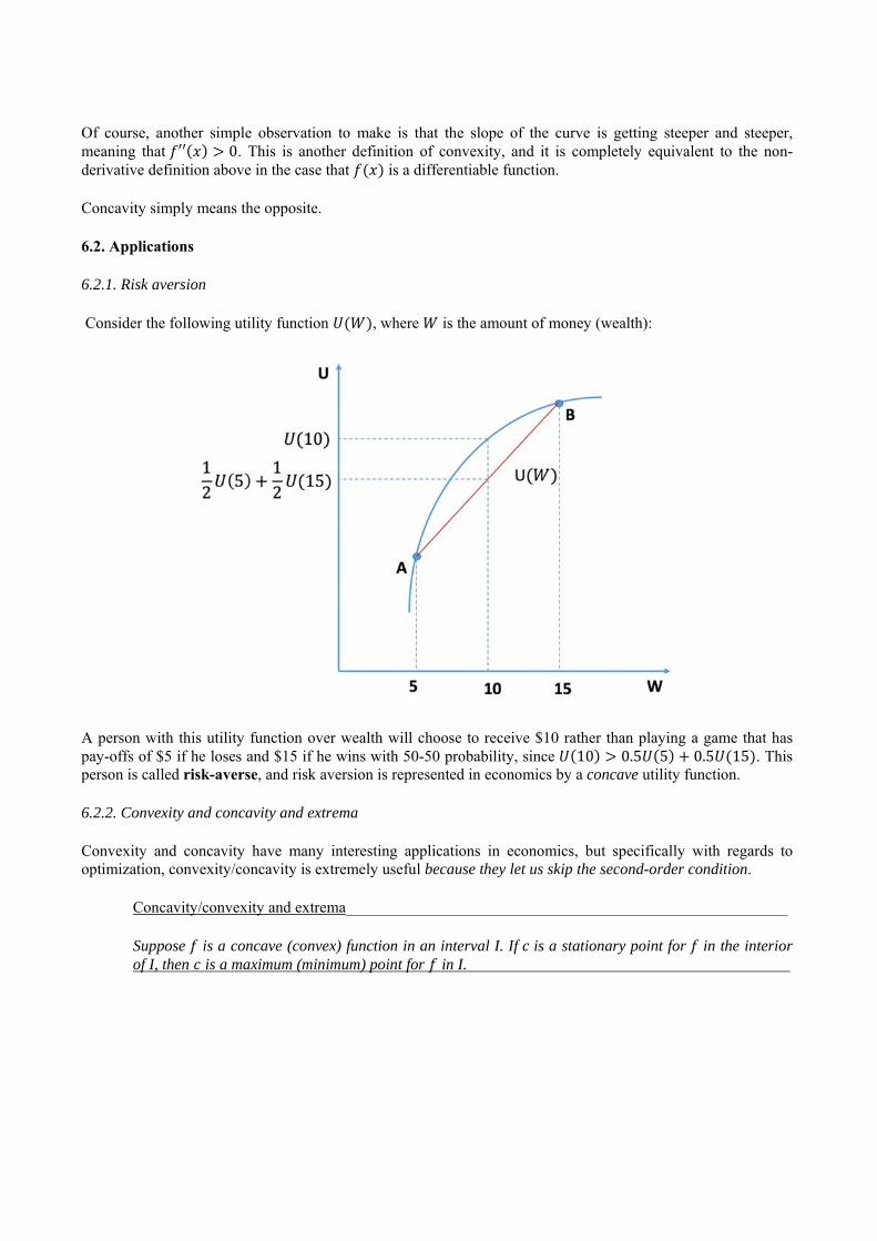
Consider the following utility function 𝑈 𝑊 , where 𝑊 is the amount of money (wealth):

A person with this utility function over wealth will choose to receive $10 rather than playing a game that has pay-offs of $5 if he loses and $15 if he wins with 50-50 probability, since 𝑈 10 0.5𝑈 5 0.5𝑈 15 . This person is called risk-averse, and risk aversion is represented in economics by a concave utility function.

6.2.2. Convexity and concavity and extrema

Convexity and concavity have many interesting applications in economics, but specifically with regards to optimization, convexity/concavity is extremely useful because they let us skip the second-order condition.

Concavity/convexity and extrema________________________________________________________

Suppose 𝑓 is a concave (convex) function in an interval I. If 𝑐 is a stationary point for 𝑓 in the interior of I, then 𝑐 is a maximum (minimum) point for 𝑓 in I.

7. Applications

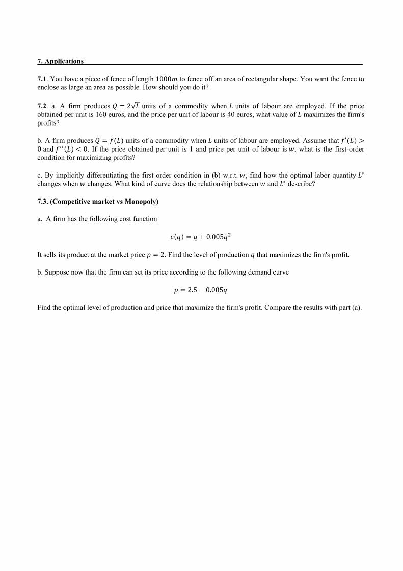
7.1. You have a piece of fence of length 1000𝑚 to fence off an area of rectangular shape. You want the fence to enclose as large an area as possible. How should you do it?

7.2. a. A firm produces 𝑄 2√𝐿 units of a commodity when 𝐿 units of labour are employed. If the price obtained per unit is 160 euros, and the price per unit of labour is 40 euros, what value of 𝐿 maximizes the firm's profits?

b. A firm produces 𝑄 𝑓 𝐿 units of a commodity when 𝐿 units of labour are employed. Assume that 𝑓′ 𝐿0 and 𝑓 𝐿 0. If the price obtained per unit is 1 and price per unit of labour is 𝑤, what is the first-order condition for maximizing profits?

c. By implicitly differentiating the first-order condition in (b) w.r.t. 𝑤, find how the optimal labor quantity 𝐿∗ changes when 𝑤 changes. What kind of curve does the relationship between 𝑤 and 𝐿∗ describe?

7.3. (Competitive market vs Monopoly)

a. A firm has the following cost function

𝑐 𝑞 𝑞 0.005𝑞

It sells its product at the market price 𝑝 2. Find the level of production 𝑞 that maximizes the firm's profit.

b. Suppose now that the firm can set its price according to the following demand curve

𝑝 2.5 0.005𝑞

Find the optimal level of production and price that maximize the firm's profit. Compare the results with part (a).

III. UNCONSTRAINED OPTIMIZATION – MULTIVARIATE CASE

1. Optimization with many control variables

Let's use an example: the profit function of a firm

𝜋 𝐾 . 𝐿 . 𝑤𝐿 𝑟𝐾

The optimization problem: choose 𝐾 and 𝐿 to maximize profit, with 𝑤 and 𝑟 given. This is an optimization problem with multiple control variables. The objective function 𝜋 is a function of 𝐿 and 𝐾, and both 𝐿 and 𝐾 are control variables.

This is the problem of finding the maximum/minimum values of a multivariate function, and we have the tools for that: partial derivatives.

2. First-order conditions

For the above example, the first-order conditions are

𝛿𝜋𝛿𝐾

0.3𝐾 . 𝐿 . 𝑟 0

𝛿𝜋𝛿𝐿

0.7𝐾 . 𝐿 . 𝑤 0

Thus, for a function of 𝑛 variables, we have 𝑛 FOCs, one for each variable.

Example: find all the stationary points for

a. 𝑧 𝑒 2𝑥 2𝑦 3

b. 𝑧 𝑒 𝑒 𝑒 2𝑥 2𝑒 𝑦

3. Second-order conditions

3.1. Functions of two variables

3.1.1. Convex sets

At this level, we need to have the condition that the domain in which the optimization takes place is a convex set.

Definition of a convex set

A set S in the xy-plane is convex if, for each pair of points P and Q in S, all the line segment between P and Q lies in S.

3.1.2. Second-order partial derivatives

Consider the function

𝑓 𝑥, 𝑦 𝑥 𝑦 𝑥𝑦

It has two partial derivatives,

𝑓 𝑥, 𝑦 2𝑥𝑦 𝑦

𝑓 𝑥, 𝑦 𝑥 3𝑥𝑦

These of course are first-order derivatives. What about second-order derivatives? Naturally, we can differentiate 𝑓 𝑥, 𝑦 and 𝑓 𝑥, 𝑦 again, w.r.t 𝑥 or 𝑦. This gives us four second-order derivatives. They are

𝑓 𝑥, 𝑦 2𝑦

𝑓 𝑥, 𝑦 2𝑥 3𝑦

𝑓 𝑥, 𝑦 2𝑥 3𝑦

𝑓 𝑥, 𝑦 6𝑥𝑦

But 𝑓 𝑥, 𝑦 𝑓 𝑥, 𝑦 , so in fact every function of two variables will have three second-order derivatives.

3.1.3. Second-order conditions

(Refer to Theorem 13.2.1 in chapter 13.)

Example: find all the extreme points and values of the following functions, check that they are maxima or minima, or neither.

a. 𝑧 𝑒 3𝑥 𝑦 3

b. 𝜋 𝐾, 𝐿 12𝐾 / 𝐿 / 1.2𝐾 0.6𝐿

3.1.4. Convexity/concavity of functions of two variables

The conditions for convexity/concavity follow exactly the second-order conditions in Theorem 13.2.1. If condition (a) is satisfied, the function is concave, and vice versa.

3.2. Function of three variables or more

3.2.1. Hessian matrix

Hessian matrix of 𝑓 𝑥 , 𝑥 is

𝐻𝑓 𝑥 , 𝑥 𝑓 𝑥 , 𝑥𝑓 𝑥 , 𝑥 𝑓 𝑥 , 𝑥

Hessian matrix of 𝑓 𝒙 , where 𝒙 𝑥 , 𝑥 ,…, 𝑥 is

)()()(

)()()(

)()()(

''''2

''1

''2

''22

''21

''1

''12

''11

xxx

xxx

xxx

nnnn

n

n

fff

fff

fff

H

Note: Hessian matrix is symmetric.

3.2.2. Conditions for local max and min

Condition Max Min 1st- order Necessary 𝑓 𝑥∗ 0 for all i 𝑓 𝑥∗ 0 for all i 2nd – order Sufficient 𝐻 𝑥∗ is ND 𝐻 𝑥∗ is PD 3rd – order Necessary 𝐻 𝑥∗ is NSD 𝐻 𝑥∗ is PSD

4. Applications

4.1. A firm produces two different kinds A and B of a commodity. The daily cost of producing x units of A and y units of B is

𝐶 𝑥, 𝑦 0.04𝑥 0.01𝑥𝑦 0.01𝑦 4𝑥 2𝑦 500

Suppose that the firm sells all its output at a price per unit of 15 for A and 9 for B. Find the daily production levels x and y that maximize profit per day.

4.2. Help Jane again: decide how much ice cream and apples to consume to maximize her utility, with the utility given as

𝑈 𝑥, 𝑦 𝑥 . 𝑦 . 0.1𝑥 0.2𝑦

4.3. (Price discrimination)

Faced with two such isolated markets, the discriminating monopolist has two independent demand curves. Suppose that, in inverse form, these are

𝑃 𝑎 𝑏 𝑄

𝑃 𝑎 𝑏 𝑄

for market areas 1 and 2, respectively.

Suppose, too, that the total cost is proportional to total production

𝐶 𝑄 𝛼 𝑄 𝑄

How will the firm maximize its profit?

IV. CONSTRAINED OPTIMIZATION – EQUALITY CONSTRAINT

1. What is constrained optimization

Let's look at the utility maximization problems faced by Jane so far: her concern is to choose the quantities of ice cream and apple to give her the maximum utility. There is no restriction on how much ice cream and how many apples she can get. In a more realistic scenario, however, Jane would face some restrictions: a budget. She is still finding out the quantities of ice cream and apples to give her the most satisfaction, but these quantities have to come from within a set of options – this is called a constraint.

2. The constrained optimization problem

2.1. Setting the problem

Let’s say Jane has the following utility function over ice cream and apples

𝑈 𝑥, 𝑦 𝑥 . 𝑦 . 𝑥: 𝑖𝑐𝑒 𝑐𝑟𝑒𝑎𝑚 𝑐𝑜𝑛𝑒𝑠, 𝑦: 𝑎𝑝𝑝𝑙𝑒𝑠

This is her objective function, and 𝑥 and 𝑦 are her control variables, same as before.

Here, additionally, Jane has a weekly budget: $50/week, while the prices of ice cream and apples are $2.5/cone and $2/apple, respectively. Clearly, Jane has to choose 𝑥 and 𝑦 so that they do not violate the budget. Expressed mathematically, her budget is

2.5𝑥 2𝑦 50

Now we can formulate the constrained optimization problem:

𝐦𝐚𝐱𝒙,𝒚

𝑼 𝒙, 𝒚 𝒙𝟎.𝟑𝒚𝟎.𝟕

subject to

𝟐. 𝟓𝒙 𝟐𝒚 𝟓𝟎

2.2. Solving the problem

2.2.1. Forming the Lagrangian

The first step is to turn the constrained optimization into an unconstrained one, by forming what we call the Lagrangian. Using the example, the Lagrangian is

𝐿 𝑥, 𝑦, 𝝀 𝑈 𝑥, 𝑦 𝝀 2.5𝑥 2𝑦 50

So the constrained optimization problem has now become

max, ,

𝐿 𝑥, 𝑦, 𝜆 𝑥 . 𝑦 . 𝜆 2.5𝑥 2𝑦 50

with the constraint gone. Now we see 𝐿 as a function of three variables, which needs to be maximized. This is just a regular multivariate optimization problem. In doing this, we introduce as new variable, 𝜆, which is called the Lagrange multiplier. We proceed to maximize/minimize the Lagrangian instead of the original objective function.

2.2.2. The first-order conditions and solutions

Using the Lagrangian as the objective function, we set up the first-order conditions and proceed to solve them for the optimal points (remember: the Lagrange multiplier is one of the control variables).

𝐿 0.3𝑥 . 𝑦 . 2.5𝜆 0

𝐿 0.7𝑥 . 𝑦 . 2𝜆 0

𝐿 2.5𝑥 2𝑦 50 0

By solving this system of 3 variables, we arrive at the values of 𝑥 and 𝑦 that maximizes the utility function (the original objective function) while respecting the constraint. Task: solve the above system of equations to get the optimal 𝑥 and 𝑦 for Jane.

Example:

a. max 𝑥𝑦 subject to 2𝑥 𝑦 𝑚

b. Cost minimization

min 𝑟𝐾 𝑤𝐿 subject to √𝐾 𝐿 𝑄

2.2.3. Sufficient conditions

a) Concave/Convex Lagrangian: Theorem 14.5.1

b) Local Second-Order Conditions:

Define |𝐻| be the determinant of the bordered Hessian matrix

Theorem: Consider the problem max min,

𝑓 𝑥, 𝑦 s. t. 𝑔 𝑥, 𝑦 𝑐. Suppose that 𝑥 , 𝑦 and 𝜆 satisfies the

first-order conditions : ℒ 𝑓 𝑥 , 𝑦 𝜆𝑔 𝑥 , 𝑦 0 ℒ 𝑓 𝑥 , 𝑦 𝜆𝑔 𝑥 , 𝑦 0 𝑔 𝑥 , 𝑦 𝑐

Then, (i) if |𝐻| 0, then 𝑥 , 𝑦 is a local max point. (ii) if |𝐻| 0, then 𝑥 , 𝑦 is a local min point. (or you can refer to Theorem 14.5.2 in textbook)

2.3. More variables and constraints

Consider the following optimization problem

max, ,

𝑈 𝑥, 𝑦, 𝑧

subject to

(i) 2.5𝑥 2𝑦 3𝑧 50 and (ii) 2𝑥 3𝑦 2𝑧 30

The Lagrangian is formed in analogous manner, with one more Lagrange multiplier for the additional constraint (thus, the number of Lagrange needed = the number of constraints):

𝐿 𝑥, 𝑦, 𝑧, 𝝀, 𝝁 𝑈 𝑥, 𝑦, 𝑧 𝝀 2.5𝑥 2𝑦 3𝑧 50 𝝁 2𝑥 3𝑦 2𝑧 30

The number of control variables is now five, so we have five F.O.Cs. Task: write down the five F.O.Cs.

Example: Solve the problem

a. max 𝑈 𝑥, 𝑦, 𝑧 𝑥 𝑦 𝑧 subject to 𝑥 𝑦 𝑧 12

b. min 𝑥 𝑦 𝑧 subject to (i) 𝑥 2𝑦 𝑧 30 and (ii) 2𝑥 𝑦 3𝑧 10

3. Applications

3.1. Utility maximization

Each week an individual consumes quantities 𝑥 and 𝑦 of two goods, and works for 𝑙 hours. These three quantities are chosen to maximize the utility function

𝑈 𝑥, 𝑦, 𝑙 𝛼 ln 𝑥 𝛽 ln 𝑦 1 𝛼 𝛽 ln 𝐿 𝑙

which is defined for 0 𝑙 𝐿 and for 𝑥, 𝑦 0. Here 𝛼 and 𝛽 are positive parameters satisfying 𝛼 𝛽 1. The individual faces the budget constraint

𝑝𝑥 𝑞𝑦 𝑤𝑙

where 𝑤 is the wage per hour. Find the individual’s demands 𝑥∗, 𝑦∗, and labour supply 𝑙∗ as functions of 𝑝, 𝑞, and 𝑤.

Let's form the Lagrangian:

𝐿 𝑥, 𝑦, 𝑙, 𝜆 𝛼 ln 𝑥 𝛽 ln 𝑦 1 𝛼 𝛽 ln 𝐿 𝑙 𝜆 𝑝𝑥 𝑞𝑦 𝑤𝑙

We have four control variables, so there will be four F.O.Cs. Task: find the four F.O.Cs and solve the system.

3.2. The consumption-saving model

Let's help Jane again, this time with some financial decision. In the current period, Jane earns 𝑦 in income, and she expects to earn 𝑦 in a future period. For each period, Jane has to spend some (or all, in the case of the second period) of her income for consumption on goods and services, denoted by 𝑐 and 𝑐 respectively. The utility she derives from consumption over the two periods is

𝑈 𝑐 , 𝑐 ln 𝑐 𝛽 ln 𝑐

where 𝛽 1.

If Jane decides to save some of her income in period 1, she earns an interest rate of 𝑟 on the saving in period 2. Help Jane decides how much to save so as to get the optimal utility from her consumption.

First, let's formulate the constraints: her budgets. In period 1, her income is split into consumption and saving, thus:

𝑐 𝑠 𝑦

In period 2, all that she has/earns is used for consumption (by assumption), thus

𝑐 1 𝑟 𝑠 𝑦

We can combine the two budgets to have

𝑐𝑐

1 𝑟𝑦

𝑦1 𝑟

Jane's optimization problem is therefore

max,

𝑈 𝑐 , 𝑐 ln 𝑐 𝛽 ln 𝑐

s.t.

𝑐𝑐

1 𝑟𝑦

𝑦1 𝑟

with 𝑦 and 𝑦 given, and 𝑟 a given parameter.

Let's form the Lagrangian

𝐿 𝑐 , 𝑐 , 𝜆 ln 𝑐 𝛽 ln 𝑐 𝜆 𝑐𝑐

1 𝑟𝑦

𝑦1 𝑟

The optimal conditions are

𝐿1𝑐

𝜆 0

𝐿𝛽𝑐

𝜆1 𝑟

0

𝐿 𝑐𝑐

1 𝑟𝑦

𝑦1 𝑟

0

Combining to get rid of 𝜆

𝑐𝑐

𝛽 1 𝑟

𝑐𝑐

1 𝑟𝑦

𝑦1 𝑟

We get the solutions

𝑐1

1 𝛽𝑦

𝑦1 𝑟

𝑐𝛽 1 𝑟

1 𝛽𝑦

𝑦1 𝑟

Let's perform some comparative static analysis. We can ask ourselves the questions:

- What happens when Jane earns more in the 1st period?

- What happens when the interest rate is higher?

Additional Material: Quadratic Forms

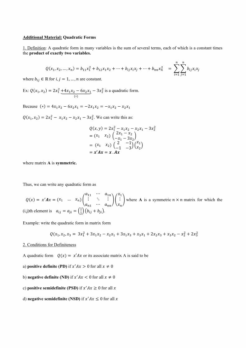
1. Definition: A quadratic form in many variables is the sum of several terms, each of which is a constant times the product of exactly two variables.

𝑄 𝑥 , 𝑥 , … , 𝑥 𝑏 𝑥 𝑏 𝑥 𝑥 ⋯ 𝑏 𝑥 𝑥 ⋯ 𝑏 𝑥 𝑏 𝑥 𝑥

where 𝑏 ∈ ℝ for 𝑖, 𝑗 1, … , 𝑛 are constant.

Ex: 𝑄 𝑥 , 𝑥 2𝑥 4𝑥 𝑥 6𝑥 𝑥∗

3𝑥 is a quadratic form.

Because ∗ 4𝑥 𝑥 6𝑥 𝑥 2𝑥 𝑥 𝑥 𝑥 𝑥 𝑥

𝑄 𝑥 , 𝑥 2𝑥 𝑥 𝑥 𝑥 𝑥 3𝑥 . We can write this as:

𝑄 𝑥, 𝑦 2𝑥 𝑥 𝑥 𝑥 𝑥 3𝑥

𝑥 𝑥 2𝑥 𝑥𝑥 3𝑥

𝑥 𝑥 2 11 3

𝑥𝑥

𝒙 𝑨𝒙 𝒙 . 𝑨𝒙

where matrix A is symmetric.

Thus, we can write any quadratic form as

𝑄 𝑥 𝑥 𝑨𝑥 𝑥 … 𝑥𝑎 ⋯ 𝑎

⋮ ⋱ ⋮𝑎 ⋯ 𝑎

𝑥⋮

𝑥 where A is a symmetric 𝑛 𝑛 matrix for which the

(i,j)th element is 𝑎 𝑎 𝑏 𝑏 .

Example: write the quadratic form in matrix form

𝑄 𝑥 , 𝑥 , 𝑥 3𝑥 3𝑥 𝑥 𝑥 𝑥 3𝑥 𝑥 𝑥 𝑥 2𝑥 𝑥 𝑥 𝑥 𝑥 2𝑥

2. Conditions for Definiteness

A quadratic form 𝑄 𝑥 𝑥′𝐴𝑥 or its associate matrix A is said to be

a) positive definite (PD) if 𝑥 𝐴𝑥 0 for all 𝑥 0

b) negative definite (ND) if 𝑥 𝐴𝑥 0 for all 𝑥 0

c) positive semidefinite (PSD) if 𝑥 𝐴𝑥 0 for all 𝑥

d) negative semidefinite (NSD) if 𝑥 𝐴𝑥 0 for all 𝑥

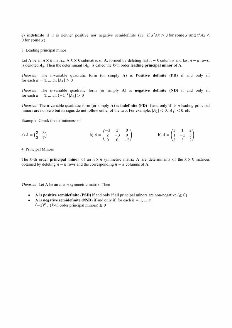
e) indefinite if it is neither positive nor negative semidefinite (i.e. if 𝑥 𝐴𝑥 0 for some 𝑥, and 𝑥 𝐴𝑥0 for some 𝑥

3. Leading principal minor

Let A be an 𝑛 𝑛 matrix. A 𝑘 𝑘 submatrix of A, formed by deleting last 𝑛 𝑘 columns and last 𝑛 𝑘 rows, is denoted 𝑨𝒌. Then the determinant |𝐴 | is called the 𝑘-th order leading principal minor of A.

Theorem: The n-variable quadratic form (or simply A) is Positive definite (PD) if and only if, for each 𝑘 1, … , 𝑛, |𝐴 | 0

Theorem: The n-variable quadratic form (or simply A) is negative definite (ND) if and only if, for each 𝑘 1, … , 𝑛, 1 |𝐴 | 0

Theorem: The n-variable quadratic form (or simply A) is indefinite (PD) if and only if its n leading principal minors are nonzero but its signs do not follow either of the two. For example, |𝐴 | 0, |𝐴 | 0, etc

Example: Check the definiteness of

a) 𝐴 2 33 7

b) 𝐴3 2 0

2 3 00 0 5

b) 𝐴3 1 21 1 32 3 2

4. Principal Minors

The 𝑘 -th order principal minor of an 𝑛 𝑛 symmetric matrix A are determinants of the 𝑘 𝑘 matrices obtained by deleting 𝑛 𝑘 rows and the corresponding 𝑛 𝑘 columns of A.

Theorem: Let A be an 𝑛 𝑛 symmetric matrix. Then

A is positive semidefinite (PSD) if and only if all principal minors are non-negative ( 0 A is negative semidefinite (NSD) if and only if, for each 𝑘 1, … , 𝑛,

1 . 𝑘-th order principal minors) 0

ECON205 Intermediate Mathematics for Economics

Lecture Notes Chapter 5. Dynamic Analysis

I. DYNAMIC ANALYSIS

In chapters 2, 3, 4, we dealt with static analysis in economics. We are interested in equilibria, how to obtain optimal equilibria, and we ignore how the economic variables get there.

In this chapter, we analyze the dynamics of the variables of interest, that is, how they change. For example, we know that the output of the economy grows over time, but how does it grow over time? If we can find how it grows with time, we can express it as a function of time, and find a specific value of it at any given time.

The main tool to use in this type of problems is integration.

II. INTEGRALS

1. Integrals

1.1. What is an integral?

At the most basic level, integrals are sums. Let's take a related example from economics: accumulation of the capital stock. How does the capital stock grow over time? By investment, such that

𝐾 𝐾 ∆𝐾 𝐼

If 𝐼 is a function of time, for example, the economy is making an investment of $2b in new capital per day, then after one year

∆𝐾 𝐼 𝑡 ∆𝑡 2 365

But if the investment is not constant, for example, $2b per day for the first half of the year, then $3b per day for the second half? Then

∆𝐾 𝐼 𝑡 ∆𝑡 𝐼 𝑡 ∆𝑡 2 182 3 183

If the investment changes every day? Then

∆𝐾 𝐼 𝑡 ∆𝑡

where ∆𝑡 1 day.

And so, assuming that the capital stock starts at 0, after a period of time, the capital stock is

𝐾 0 ∆𝐾 𝐼 𝑡 ∆𝑡

where ∆𝑡 is the interval of time within which 𝐼 𝑡 is constant.

What if 𝐼 𝑡 is continuous, that is, it changes constantly with time? In this case, we can't find ∆𝑡 such that within it 𝐼 𝑡 stays constant. We can only approximate. We can use the above summation to approximate 𝐾, and the approximation is poor if the time interval ∆𝑡 is large. What is the graphical representation of this?

To make the summation a better approximation, we need to shrink ∆𝑡. As ∆𝑡 → 0,

𝐾 𝑡 lim∆ →

𝐼 𝑡 ∆𝑡 𝐼 𝑡 𝑑𝑡

We call 𝐾 𝑡 loosely the integral of 𝐼 𝑡 .

In general, the integral of a function 𝑓 𝑥 is

𝑓 𝑥 𝑑𝑥 lim∆ →

𝑓 𝑥 ∆𝑥

Think of the term 𝑓 𝑥 𝑑𝑥 as just 𝑓 𝑥 𝑑𝑥, which is the area of the rectangle with sides 𝑓 𝑥 and 𝑑𝑥. The integral of 𝑓 𝑥 is thus a sum of the rectangles 𝑓 𝑥 𝑑𝑥, with the side 𝑑𝑥 becoming vanishingly small.

1.2. Indefinite integrals

At the practical level, integrals are the just the opposite of derivatives.

Definition of indefinite integrals

𝐹 𝑥 𝑓 𝑥 ⟺ 𝑓 𝑥 𝑑𝑥 𝐹 𝑥 𝐶

1.3. Definite integrals

Definition of definite integrals

𝐼𝑓 𝐹 𝑥 𝑓 𝑥 , 𝑓 𝑥 𝑑𝑥 𝐹 𝑥 𝐹 𝑏 𝐹 𝑎

Think of definite integrals as calculating the area under a curve.

1.4. Some application of integrals

Example 1: finding average

In a country, citizen incomes follow the following distribution 𝑓 𝑟 𝐵/𝑟 . , where 𝑟 is income, 𝑓 𝑟 is the income density function. Find the mean income for the group of people with incomes between 𝑎 and 𝑏.

Example 2: capital stock and investment

If 𝐼 𝑡 3𝑡 / , what is the amount of capital accumulated by time 𝑡 ? What is the amount of capital accumulated between 𝑡 1 and 𝑡 3?

2. Rules of integrals

𝑎𝑓 𝑥 𝑑𝑥 𝑎 𝑓 𝑥 𝑑𝑥

𝑓 𝑥 𝑔 𝑥 𝑑𝑥 𝑓 𝑥 𝑑𝑥 𝑔 𝑥 𝑑𝑥

𝑓 𝑥 𝑑𝑥 𝑓 𝑥 𝑑𝑥

𝑓 𝑥 𝑑𝑥 0

𝛼𝑓 𝑥 𝑑𝑥 𝛼 𝑓 𝑥 𝑑𝑥

𝑓 𝑥 𝑑𝑥 𝑓 𝑥 𝑑𝑥 𝑓 𝑥 𝑑𝑥

3. Techniques of integration (Textbook Chapter 9.1, 9.5, 9.6)

3.1. Integrating basic functions

3.2. Integration by parts

3.3. Integration by substitution

3.4. Examples

a) 𝑥𝑒 𝑑𝑥 b) ln 𝑥 𝑑𝑥

c) 8𝑥 3𝑥 1 𝑑𝑥 d) 𝑑𝑥

4. Applications

4.1. From marginal to total

Example: With 𝐶 𝑌 as the consumption function, suppose the marginal propensity to consume is 𝐶 𝑌0.69, with 𝐶 0 1000. Find 𝐶 𝑌 .

Example: In the manufacture of a product, the marginal cost of producing x units is 𝐶 𝑥 𝛼𝑒 𝛾, with 𝛽 0, and fixed costs are 𝐶 . Find the total cost function 𝐶 𝑥 .

4.2. Consumer and producer surplus

Suppose the demand and supply curves are 𝑃 𝑓 𝑄 6000/ 𝑄 50 , 𝑃 𝑔 𝑄 𝑄 10. Find the equilibrium price and quantity, and compute the consumer and producer surplus.

4.3. Total present value

Recall the present value of a single future payment 𝐴 𝑡 periods of time in the future:

𝑃𝑉𝐴

1 𝑟

Continuously,

𝑃𝑉 𝐴𝑒

(Note: the interest rate 𝑟 has to be consistent with the time duration 𝑡 is counted in. For example, if it is 𝑡 years, the interest rate has to be an annual interest rate.)

Now suppose we have multiple payments at the end of each period of time until 𝑡 periods of time in the future. The total present value of this stream of payments is:

𝑇𝑃𝑉𝐴

1 𝑟𝐴

1 𝑟. . .

𝐴1 𝑟

Now suppose that this stream of future payments is continuous, that is 𝐴 is a function of time 𝐴 𝑡 . Over any small interval of time, the amount of payment is (approximately) 𝐴 𝑡 𝑑𝑡, and its discounted value to the present is

𝑑𝑃𝑉 𝐴 𝑡 𝑒 𝑑𝑡

Thus, the total present value of a continuous stream of future payments is simply the sum of all these 𝑑𝑃𝑉, which is an integral:

𝑇𝑃𝑉 𝑑𝑃𝑉𝑑𝑡 𝐴 𝑡 𝑒 𝑑𝑡

Example: Consider a tree that is planted at time 𝑡 0, and let 𝑃 𝑡 be its current market value at time 𝑡, where 𝑃 𝑡 is differentiable with 𝑃 𝑡 0 for all 𝑡 0. Assume that the interest rate is 100𝑟% per year, and assume continuous compounding of interest.

(a) At what time 𝑡∗ should this tree be cut down in order to maximize its present value?

(b) The optimal cutting time 𝑡∗ depends on the interest rate r. Find 𝑑𝑡∗/𝑑𝑟 .

III. DIFFERENTIAL EQUATIONS

1. Differential equations

1.1. Separable DEs

Different equations are separate if they are in this form

𝑑𝑥𝑑𝑡

𝑓 𝑡 𝑔 𝑥

meaning that they can be re-arranged

𝑑𝑥𝑔 𝑥

𝑓 𝑡 𝑑 𝑡

and be solved by integrating each side

𝑑𝑥𝑔 𝑥

𝑓 𝑡 𝑑 𝑡

Example 1: solve the following DE

𝑑𝑥𝑑𝑡

𝑒ln 𝑥

Example 2: Let 𝑆 𝑡 denote the sales volume of a particular commodity per unit of time, evaluated at time 𝑡. In a stable market where no sales promotion is carried out, the decrease in 𝑆 𝑡 per unit of time is proportional to 𝑆 𝑡 . Thus sales decelerate at the constant proportional rate 𝑎 0, implying that

𝑑𝑆 𝑡𝑑𝑡

𝑎𝑆 𝑡

a. Find an expression for 𝑆 𝑡 , given that sales at time 0 are 𝑆 .

b. Find the time it takes before sales fall to half their initial level.

1.2. Linear DEs

Linear differential equations are differential equations in which the time differentials of the time-varying variable appear in linear terms. In this course, we limit the scope to first-order LDEs, equations that involve only the first-order differentials of the time-varying variable.

1.2.1. First-order LDEs with constant terms

𝑑𝑥𝑑𝑡

𝑎𝑥 𝑏

Solving this is simply a case of rearranging the equation into

𝑑𝑥𝑑𝑡

𝑏 𝑎𝑥

which is separable

𝑑𝑥𝑏 𝑎𝑥

𝑑𝑡

1.2.2. First-order LDEs with functional terms

𝑑𝑥𝑑𝑡

𝑎𝑥 𝑏 𝑡

To solve this type of DEs, we need to use something called the integrating factor. We multiply both sides of the equation with 𝑒 , so that

𝑒𝑑𝑥𝑑𝑡

𝑎𝑥𝑒 𝑏 𝑡 𝑒

which is

𝑑𝑑𝑡

𝑥𝑒 𝑏 𝑡 𝑒

Thus

𝑥𝑒 𝑏 𝑡 𝑒 𝑑𝑡 𝐶

and

𝑥 𝑒 𝑏 𝑡 𝑒 𝑑𝑡 𝐶𝑒

Example: find the solution of

𝑑𝑥𝑑𝑡

𝑥 𝑡

2. Applications

2.1. Economic Growth 1

Let 𝑌 𝑌 𝑡 denote the national product (output), 𝐾 𝐾 𝑡 the capital stock, and 𝐿 𝐿 𝑡 the number of workers in a country at time t. Suppose that, for all t ≥ 0,

(a) 𝑌 √𝐾√𝐿 (b) 0.4𝑌 (c) 𝐿 𝑒 .

Derive from these equations a single differential equation for 𝐾 𝐾 𝑡 , and find the solution of that equation when 𝐾 0 10000. (In (a) we have a Cobb–Douglas production function, (b) says that aggregate investment is proportional to output, whereas (c) implies that the labour force grows exponentially.)

We have all the ingredients to find a differential equation for 𝐾 𝑡 :

𝑑𝐾𝑑𝑡

0.4√𝐾𝑒 .

This is a separable DE:

𝑑𝐾

√𝐾0.4𝑒 . 𝑑𝑡

2𝐾0.4

0.02𝑒 . 𝐶

𝐾 10𝑒 . 𝐶/2

Given 𝐾 0 10000, thus

𝐶2

90

So,

𝐾 10𝑒 . 90

2.2. Economic Growth 2

Consider the following model of economic growth in a developing country

(a) 𝑌 𝑡 0.2𝐾 𝑡 (b) 0.1𝑌 𝑡 𝐻 𝑡 (c) 𝑁 𝑡 50𝑒 .

Here 𝑌 𝑡 is total domestic product (output) per year, 𝐾 𝑡 is capital stock, 𝐻 𝑡 is the net inflow of foreign investment per year, and 𝑁 𝑡 is the size of the population, all measured at time 𝑡. In (a) we assume that output is simply proportional to the capital stock, with the factor of proportionality 0.2 called the average productivity of capital. In (b) we assume that the total growth of capital per year is equal to internal savings plus net foreign investment. We assume that savings are proportional to output, with the factor of proportionality 0.1 called the savings rate. Finally, (c) tells us that population increases at a constant proportional rate of growth 0.03.

Assume that 𝐻 𝑡 10𝑒 . , and derive from these equations a differential equation for 𝐾 𝑡 . Find its solution given that 𝐾 0 200. Find also an expression for 𝑦 𝑡 𝑌 𝑡 /𝑁 𝑡 , which is output per capita.

Again, the differential equation for 𝐾 𝑡 is easily found

𝑑𝐾𝑑𝑡

0.02𝐾 10𝑒 .

or

𝑑𝐾𝑑𝑡

0.02𝐾 10𝑒 .

Solving it using the integrating factor:

𝑒 . 𝑑𝐾𝑑𝑡

0.02𝐾𝑒 . 10𝑒 . 𝑒 .

𝐾𝑒 . 100.02

𝑒 . 𝐶

𝐾 500𝑒 . 𝐶𝑒 .

𝐾 0 200 gives:

𝐾 0 200 500 𝐶 ⇒ 𝐶 300

Thus

𝐾 500𝑒 . 300𝑒 .

Output per capita is

𝑦 𝑡𝑌 𝑡𝑁 𝑡

0.2𝐾 𝑡50𝑒 .

0.2 500𝑒 . 300𝑒 .

50𝑒 . 2𝑒 . 1.2𝑒 .

2.3. Price adjustment

Let 𝐷 𝑃 𝑎 𝑏𝑃 denote the demand quantity and 𝑆 𝑃 𝛼 𝛽𝑃 the supply of a certain good. Here 𝑎, 𝑏, 𝛼, and 𝛽 are positive constants. Assume that the price 𝑃 𝑃 𝑡 varies with time, and its rate of adjustment is proportional to excess demand 𝐷 𝑃 𝑆 𝑃 . Thus,

𝑑𝑃𝑑𝑡

𝜆 𝐷 𝑃 𝑆 𝑃

Solve for 𝑃 𝑡 .

We have

𝑑𝑃𝑑𝑡

𝜆 𝑎 𝑏𝑃 𝛼 𝛽𝑃

𝑑𝑃𝜆 𝑎 𝑏𝑃 𝛼 𝛽𝑃

𝑑𝑡

Solving for 𝑃

𝑑𝑃𝜆 𝑎 𝑏𝑃 𝛼 𝛽𝑃

𝑑𝑡

ln 𝜆 𝑎 𝑏𝑃 𝛼 𝛽𝑃𝜆 𝑏 𝛽

𝑡 𝐶

ln 𝜆 𝑎 𝑏𝑃 𝛼 𝛽𝑃 𝜆 𝑏 𝛽 𝑡 𝐶

𝜆 𝑎 𝑏𝑃 𝛼 𝛽𝑃 𝑒

𝜆 𝑎 𝑏𝑃 𝛼 𝛽𝑃 𝑒 𝑒

𝑃𝐴

𝜆 𝑏 𝛽𝑒

𝑎 𝛼𝑏 𝛽

Remarks: since 𝜆 𝑏 𝛽 0, as 𝑡 tends to infinity, 𝑃 converges to the equilibrium value . Thus, we called

this equilibrium dynamically stable, because the time process of the price variable is not explosive.