Embed Size (px)
Citation preview
Ecole normale superieure de Lyon
Laboratoire de l’Informatique du Parallelisme
Ecole Doctorale Informatique et Mathematiques
Doctorat
Informatique
Benoit BOISSINOT
Towards an SSA based compiler back-end:some interesting properties of SSA and its
extensions
These dirigee par Fabrice RASTELLO.
Soutenue le 30 septembre 2010.
Jury:
Albert Cohen (Rapporteur)Anton Ertl (Examinateur)David Monniaux (Rapporteur)Fabrice Rastello (Directeur)Yves Robert (Examinateur)
2
Contents
1 Introduction 5
2 Control flow graph, loops, and SSA 9
2.1 Control flow graph (CFG) . . . . . . . . . . . . . . . . . . . . 9
2.1.1 Definitions and properties . . . . . . . . . . . . . . . . 9
2.1.2 Traversal and order of CFG . . . . . . . . . . . . . . . 11
2.2 Loops . . . . . . . . . . . . . . . . . . . . . . . . . . . . . . . 14
2.2.1 Definition . . . . . . . . . . . . . . . . . . . . . . . . . 14
2.2.2 Minimal connected loop nesting forest . . . . . . . . . 15
2.3 Join set . . . . . . . . . . . . . . . . . . . . . . . . . . . . . . 17
2.4 Static single assignment (SSA) form . . . . . . . . . . . . . . . 17
2.4.1 Definitions . . . . . . . . . . . . . . . . . . . . . . . . . 17
2.4.2 Minimal SSA . . . . . . . . . . . . . . . . . . . . . . . 18
2.4.3 Liveness and variants of SSA form . . . . . . . . . . . . 19
3 Liveness analysis under SSA 21
3.1 Definitions . . . . . . . . . . . . . . . . . . . . . . . . . . . . . 22
3.2 Liveness set . . . . . . . . . . . . . . . . . . . . . . . . . . . . 22
3.2.1 Classical liveness set construction . . . . . . . . . . . . 24
3.2.2 Two pass data flow . . . . . . . . . . . . . . . . . . . . 26
3.2.3 One variable at a time . . . . . . . . . . . . . . . . . . 29
3.2.4 One use at a time . . . . . . . . . . . . . . . . . . . . . 30
3.3 Liveness check . . . . . . . . . . . . . . . . . . . . . . . . . . . 33
3.4 From reducible CFG to irreducible CFG . . . . . . . . . . . . 35
3.5 Interference . . . . . . . . . . . . . . . . . . . . . . . . . . . . 39
3.6 Conclusion . . . . . . . . . . . . . . . . . . . . . . . . . . . . . 42
3
4 CONTENTS
4 SSA extensions: SSI 434.1 Definitions and motivations . . . . . . . . . . . . . . . . . . . 43
4.1.1 Ananian’s definition of SSI . . . . . . . . . . . . . . . . 434.1.2 Singer’s definition of SSI . . . . . . . . . . . . . . . . . 464.1.3 Semi-pruned and pruned SSI form . . . . . . . . . . . . 46
4.2 Weak and strong SSI forms . . . . . . . . . . . . . . . . . . . 474.2.1 Weak and strong SSI forms are not equivalent . . . . . 484.2.2 Properties of variables in weak and strong SSI forms . 49
4.3 The intersection graph is an interval graph . . . . . . . . . . . 504.3.1 Strong SSI form . . . . . . . . . . . . . . . . . . . . . . 514.3.2 Weak SSI form . . . . . . . . . . . . . . . . . . . . . . 55
4.4 Liveness under SSI . . . . . . . . . . . . . . . . . . . . . . . . 604.5 Single-entry single-exit region and SSI . . . . . . . . . . . . . 61
4.5.1 Single-entry single-exit region . . . . . . . . . . . . . . 634.5.2 Removal of σ-functions . . . . . . . . . . . . . . . . . . 65
5 SSA Destruction 695.1 Motivations . . . . . . . . . . . . . . . . . . . . . . . . . . . . 695.2 Clean approach . . . . . . . . . . . . . . . . . . . . . . . . . . 71
5.2.1 Going out of CSSA: a coalescing problem . . . . . . . . 755.2.2 Overview of the SSA destruction . . . . . . . . . . . . 775.2.3 Coalescing . . . . . . . . . . . . . . . . . . . . . . . . . 785.2.4 Sequentialization of parallel copies . . . . . . . . . . . 795.2.5 Qualitative experiments . . . . . . . . . . . . . . . . . 80
5.3 Towards a more efficient algorithm . . . . . . . . . . . . . . . 845.3.1 Live-range intersection tests . . . . . . . . . . . . . . . 855.3.2 Linear interference test between two congruence classes,
with extension to equalities . . . . . . . . . . . . . . . 855.3.3 Virtualization of φ-nodes . . . . . . . . . . . . . . . . . 905.3.4 Results in terms of speed and memory footprint . . . . 91
5.4 Conclusion . . . . . . . . . . . . . . . . . . . . . . . . . . . . . 94
6 Conclusion 976.1 Liveness . . . . . . . . . . . . . . . . . . . . . . . . . . . . . . 976.2 Static Single Information form . . . . . . . . . . . . . . . . . . 986.3 SSA destruction . . . . . . . . . . . . . . . . . . . . . . . . . . 986.4 Perspectives . . . . . . . . . . . . . . . . . . . . . . . . . . . . 99
Chapter 1
Introduction
Compilation of programs, that is the transformation of human generatedsource code into binary code executable by a processor has always been a veryactive topic in computer science. First the goal was to get rid of the burdenof hand-compiling, letting programs themselves take care of this tedious task.The initial focus was purely on getting a correct translation from textualsource into binary code: an important area of research was lexing (separatingthe input into tokens) and parsing (interpreting the tokens). The automationbrought by the compilers can be used to optimize programs too: detectingnon-optimal structure, removing unneeded code and in general generatingthe best possible assembly for a given source code.
One of the recent trend in the compiler community is the area of virtualiza-tion. Virtualizing the program, for example by using a machine-independentbytecode to represent the compiled program, helps in several areas: portabilitybetween architectures, security, productivity, . . . While this process has beenused for a long time in the desktop and server computing field, it has onlysince recently been brought forward on embedded platforms. Indeed, thediversity of the architectures is a nightmare when it comes to distributing theexecutable, shipping a single binary that is compiled on the host processor(ahead-of-time or just-in-time compilation) helps solve this problem. But asthe host processor has limited resources, we need to design compiler algo-rithms which aggressively optimize but still run relatively fast and consumelittle memory.
Our goal is to split the compilation process, a first architecture-independentpass compiles the source code into bytecode, optimizing as much as possible.A second pass, on the host processor, then compiles the bytecode down to the
5
6 CHAPTER 1. INTRODUCTION
instructions available for the specific architecture. This second pass is severelyconstrained by the computing power available on the embedded platform, thisis the part our thesis improves by bringing new fast algorithms for crucialparts of the compiling process.
All along this process, several intermediate representation of the code canbe used. One of them is the Static Single Assignment (SSA) form, whichfacilitates some optimizations or analyses.
Under the SSA form, the program is transformed into a semantically equiv-alent program where every variable is defined only once textually. Currently,the majority of compilers use the SSA form: LLVM, GCC, Open64, . . .
Our work in this thesis is articulated around three contributions.In the first chapter, we define the ground material used in the thesis. First
we define the data structure used to represent the program, the control flowgraph, furthermore we describe some useful graph properties. Then, in thecontext of control flow graphs, we give the definition of loops, one of the mostessential structure of a computer program. Finally we define the SSA form,which is the intermediate representation at the center of this thesis.
When compiling on a resource-constrained platform, the compiling processis simplified as much as possible. Liveness analysis then becomes one of thecostliest analyses found during code generation. The second chapter presentsour fast algorithm for the liveness analysis suitable for programs in SSAform. We present several approaches, some based on path exploration, andour approach based on the structure of the loops. Since our algorithm onlyexploits the shape of the control flow graph, it does not require any complexre-computation after small modifications of the program (for example due toan optimization).
We then present a variant of the SSA form, the Static Single Information(SSI) form. In a first part, we clarify the various definitions found in theliterature, and show the differences between them. Then we prove that theintersection graph of the live-ranges of variables under SSI form is an intervalgraph. Additionally we exhibit an order of the control flow graph such thatevery live-range is an interval of the program.
Our last contribution is a clean way to go out of the SSA form. The SSAform introduces φ-functions which do not map into generated code. In orderto produce machine code, those special instructions need to be removed, byintroducing new copies, as few as possible. We present a clean process forthis transformation, clearly separating the different phases of the algorithm:first the introduction of new copies in order to reach a variant of the SSA
7
form where the φ-functions can be naturally removed, and then minimize thenumber of copies, while keeping the code under this SSA form variant. Thisapproach allows us to get a provably correct transformation, contrary to someof the previous approaches. Furthermore, while simpler to implement, ourapproach can achieve results comparable to some of the complex previoustechniques.

8 CHAPTER 1. INTRODUCTION
Chapter 2
Control flow graph, loops, andSSA
Throughout this thesis, we will use different concepts and properties. In thischapter, we lay out the groundwork needed for our contributions. We firstdescribe the internal representation of the compiler we will manipulate allalong, a graph based representation of the program: the control flow graph.Based on this representation, we define several graph relations: dominanceand post-dominance, additionally we state several useful theorems relatedto those relations. In the context of the control flow graph, we then give ageneral definition of loops, later on we define our own more specific definitionthat will prove useful in the following chapters. Finally, we define the staticsingle assignment form, a commonly used intermediate representation.
Since we only define the structures and properties which are useful forthis thesis, the interested reader can find an in-depth introduction to thistopics in most compiler textbooks. In particular, we recommend the ModernCompiler Implementation books [3] by A. Appel and J. Palsberg.
2.1 Control flow graph (CFG)
2.1.1 Definitions and properties
Control-flow graph
A procedure is represented as a control-flow graph (CFG), which is adirected graph G = (V,E, r, t), with set of nodes V , set of edges E, and two
9
10 CHAPTER 2. CONTROL FLOW GRAPH, LOOPS, AND SSA
specific nodes r and t: r is the entry node, with no incoming edge, and t isthe exit node, with no outgoing edge.
A path P of length k ≥ 0 from a node u to a node v in V is a non-emptysequence (v0, v1, . . . , vk) of nodes such that u = v0, v = vk, and (vi−1, vi) ∈ Efor i ∈ [1..k]. With this definition, a path of length 0 is a path with one nodeand no edge. If the CFG contains a self-edge, i.e., an edge of the form (u, u),then there is also a path of length 1 from u to itself. Node v is reachablefrom u if there is a path from u to v in the CFG. A node u part of a path P ,will be denoted u ∈ P . Our notion of reachability is purely static and onlydepends on the shape of the control flow graph, it does not take into accountthe execution of the program: even if a node is reachable from the start of theprogram, it does not mean there exists an input where the node is executed.
Using this purely static definition of reachability, we assume that everynode is reachable from r, this means that unreachable basic blocks havebeen pruned from the program. Every time the post-dominance property, asdefined below, will be used, we will assume that every basic block can reachthe exit of the procedure. This is not always the case, for example ”noreturn”procedures, which contain an infinite loop, do not fulfill this property. But,in order to fulfill this property, we can always add artificial edges to the CFG,even if in practice they will not be traversed during the execution.
Usually, each node in the CFG represents a basic block, i.e., a sequenceof successive instructions in the program with no branches or branch targetsinterleaved. In order to simplify definitions and proofs, we will sometimesassume that every node consists of a single instruction.
Dominance and post-dominance property
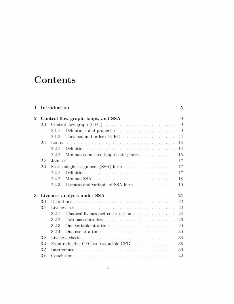
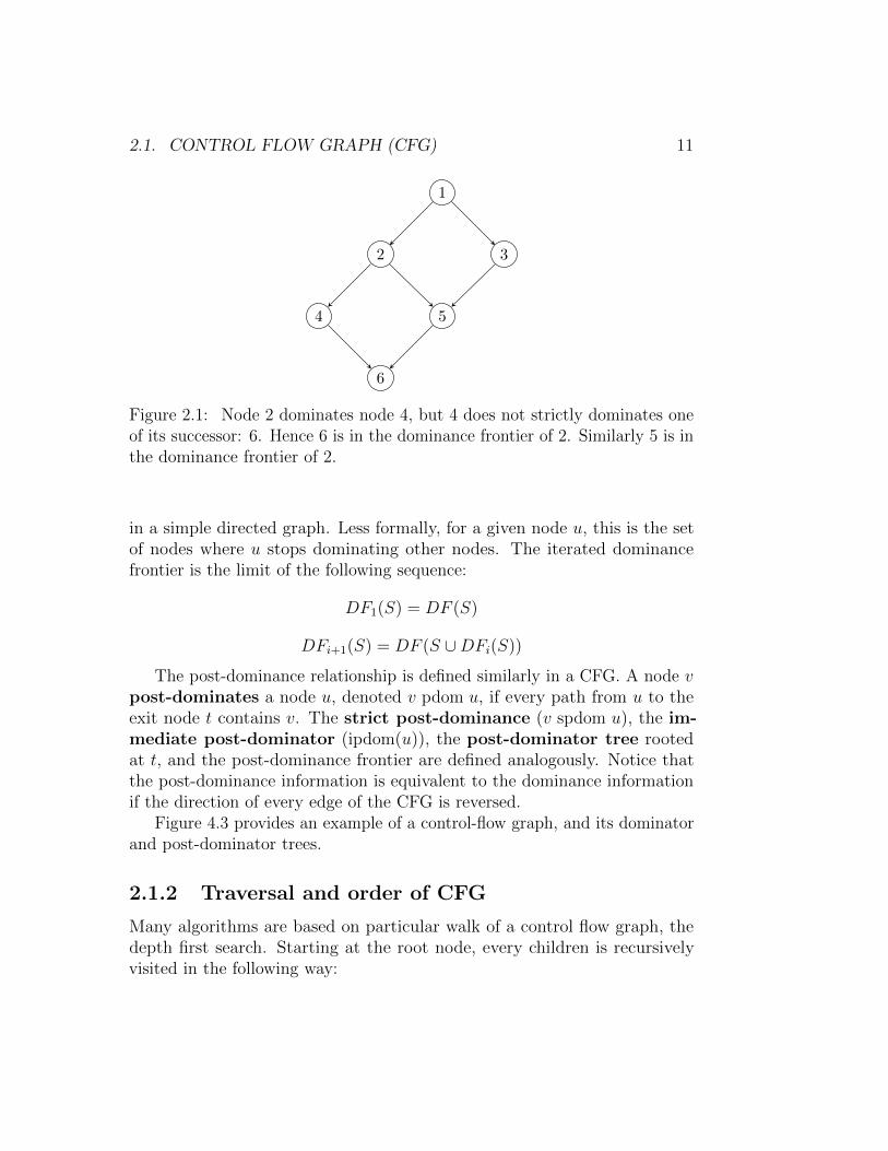
A node u in a CFG dominates a node v, denoted u dom v, if every pathfrom the entry node r to v contains u. If u dom v and u 6= v, then u strictlydominates v, denoted u sdom v. The node u is the immediate dominatorof v, denoted idom(v), if u sdom v and there exists no node w such thatu sdom w and w sdom v. Every CFG node other than r has a uniqueimmediate dominator. The directed graph whose nodes are the nodes of theCFG and in which each node other than r is pointed to by its immediatedominator is a tree rooted at r, called the dominator tree. The dominancefrontier of a set of nodes S, denoted DF (S) is the set of nodes v such thatthere exists u ∈ S, u does not strictly dominate v but dominates a predecessorof v. Figure 2.1 provides an example for the dominance frontier of a node
2.1. CONTROL FLOW GRAPH (CFG) 11
1
2 3
4 5
6
Figure 2.1: Node 2 dominates node 4, but 4 does not strictly dominates oneof its successor: 6. Hence 6 is in the dominance frontier of 2. Similarly 5 is inthe dominance frontier of 2.
in a simple directed graph. Less formally, for a given node u, this is the setof nodes where u stops dominating other nodes. The iterated dominancefrontier is the limit of the following sequence:
DF1(S) = DF (S)
DFi+1(S) = DF (S ∪DFi(S))
The post-dominance relationship is defined similarly in a CFG. A node vpost-dominates a node u, denoted v pdom u, if every path from u to theexit node t contains v. The strict post-dominance (v spdom u), the im-mediate post-dominator (ipdom(u)), the post-dominator tree rootedat t, and the post-dominance frontier are defined analogously. Notice thatthe post-dominance information is equivalent to the dominance informationif the direction of every edge of the CFG is reversed.
Figure 4.3 provides an example of a control-flow graph, and its dominatorand post-dominator trees.
2.1.2 Traversal and order of CFG
Many algorithms are based on particular walk of a control flow graph, thedepth first search. Starting at the root node, every children is recursivelyvisited in the following way:
12 CHAPTER 2. CONTROL FLOW GRAPH, LOOPS, AND SSA
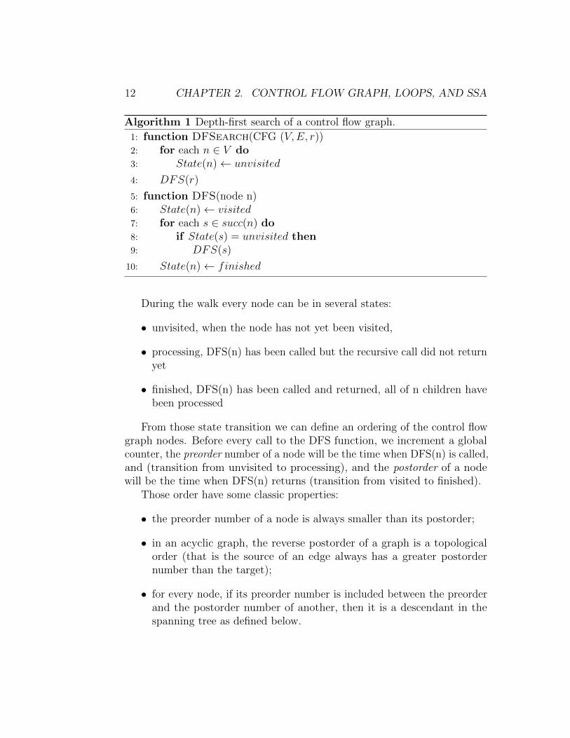
Algorithm 1 Depth-first search of a control flow graph.
1: function DFSearch(CFG (V,E, r))2: for each n ∈ V do3: State(n)← unvisited
4: DFS(r)
5: function DFS(node n)6: State(n)← visited7: for each s ∈ succ(n) do8: if State(s) = unvisited then9: DFS(s)
10: State(n)← finished
During the walk every node can be in several states:
• unvisited, when the node has not yet been visited,
• processing, DFS(n) has been called but the recursive call did not returnyet
• finished, DFS(n) has been called and returned, all of n children havebeen processed
From those state transition we can define an ordering of the control flowgraph nodes. Before every call to the DFS function, we increment a globalcounter, the preorder number of a node will be the time when DFS(n) is called,and (transition from unvisited to processing), and the postorder of a nodewill be the time when DFS(n) returns (transition from visited to finished).
Those order have some classic properties:
• the preorder number of a node is always smaller than its postorder;
• in an acyclic graph, the reverse postorder of a graph is a topologicalorder (that is the source of an edge always has a greater postordernumber than the target);
• for every node, if its preorder number is included between the preorderand the postorder number of another, then it is a descendant in thespanning tree as defined below.
2.1. CONTROL FLOW GRAPH (CFG) 13
A DFS walk of the control flow graph defines a spanning tree of the controlflow graph, if we only keep the edges which are followed. From this spanningtree, we can classify the edges in three categories:
• tree edge, going from a node in the spanning tree, to one of its successorin the spanning tree,
• forward edge, going from a node in the spanning tree, to one of itsdescendant in the spanning tree,
• cross edge, going from a node in the spanning tree, to another branch,
• back-edge, from a node to one of its ancestor in the spanning tree.
The graph obtained by removing the back-edges from a control flow graphis an acyclic graph. Furthermore, as we will see later, those back-edges playa role in loop structure.
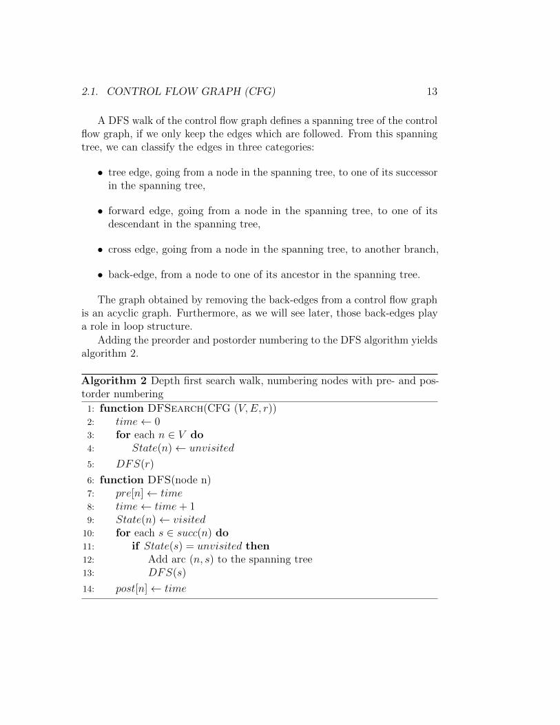
Adding the preorder and postorder numbering to the DFS algorithm yieldsalgorithm 2.
Algorithm 2 Depth first search walk, numbering nodes with pre- and pos-torder numbering
1: function DFSearch(CFG (V,E, r))2: time← 03: for each n ∈ V do4: State(n)← unvisited
5: DFS(r)
6: function DFS(node n)7: pre[n]← time8: time← time+ 19: State(n)← visited
10: for each s ∈ succ(n) do11: if State(s) = unvisited then12: Add arc (n, s) to the spanning tree13: DFS(s)
14: post[n]← time
14 CHAPTER 2. CONTROL FLOW GRAPH, LOOPS, AND SSA
2.2 Loops
Intuitively, a cycle in the control flow graph represents a loop, a sequence ofinstructions which can be repeated during the execution of the program.
2.2.1 Definition
A control flow graph can be more or less structured, for example the use ofgoto in the source language can create arbitrary control flow, while if only if,for or while are used to drive the control flow of the program, the resultingcontrol flow graph is more structured. More precisely, a set of nodes X issaid to be strongly connected if there exists a path, with only nodes from X,between any two nodes from X. A more formal definition of structured isthat a control flow graph is said to be reducible if every strongly connectedcomponent possess a node that dominates every node from the component.
While the definition for loops in reducible control flow graphs is uniqueamong the literature (since we can uniquely identify the entry of the loop),multiple definitions have been proposed to define loops in non-reducibleCFGs. Ramalingam in [27] presents a definition for loops which generalizesthe previous definitions of loops in the non-reducible case. We will presentand use this more general definition.
A loop, denoted (B,H), consists of a strongly connected component: theloop body B, and a non-empty set of distinguished nodes from the body: theheaders H. The loop will need to satisfy other properties, the first is thenesting property, two loops from a program should either be disjoint or benested. This allows us to define relations between loops, every nested loophave a unique parents, and the set of loops from the program form a forest.For the header of the loop, if the loop is reducible (intuitively, if there is aunique entry node for the loop), all definitions agree: there is a unique header,the entry node. In other cases, different choices are possible, Ramalingamproposes a definition that covers all previously proposed possibilities.
Let Entries(X), denote the entry nodes from X, that is the nodes fromX which have at least one predecessor not in X. And let UnDominated(X),denote the set of nodes from X, such that no node from X strictly dominatesthem. Obviously Entries(X) ⊂ UnDominated(X). In general, the headerswill be picked among the un-dominated nodes from the loop body. For reasonswhich will become clearer in 2.2.2, if instead of picking the headers fromUnDominated, they are chosen out of Entries, we will say that the loop
2.2. LOOPS 15
forest is connected.The set of loops we choose must cover every possible strongly connected
component from the graph. First we define the notion of cover: a loop (B,H)covers a set of nodes X, iff X ⊂ B and B∩H 6= ∅. We then add the followingrequirement: decomposition of a CFG in loops, for every strongly connectcomponent of the CFG, there exists a loop that covers it.
Ramalingam [27] gives a constructive proof of existence of minimal loopforest, which holds as long as the function used to select the headers from astrongly connected component satisfies the property that the sets are non-empty, and are a subset of UnDominated. The construction works in thefollowing way: each step of the decomposition computes a set of SCCs, whichform a new level of loops in the loop nesting forest. From this loops, headersare chosen according to the cover and Undominated property. Then, for eachsuch loop L, the loop-edges, i.e., the edges from a node in L to a loop-headerof L, are removed. This process iterates until no strongly component is left.
Since for every strongly connected component, Entries ⊂ UnDominatedand Entries 6= ∅, a connected loop forest is also a valid loop forest.
We previously defined the back-edge, in term of a spanning tree (impliedby a depth-first search) of a control flow graph. Given a set of loops, wedefine loop-edges as the set of edges (a, b), such that there exists a loop (B,H)with a ∈ B and b ∈ H, in other words, an edge from a node in the loop toone of its header. Obviously, for reducible graphs, back-edges and loop-edgesdesignate the same thing. But for non-reducible graphs they can be different.
A minimal loop nesting forest is a loop nesting forest such that no loopbody from the forest is covered by another loop. Such loop nesting forestsholds interesting properties, for example every two sets of headers are disjoint(a node can only be a header of one loop).
Figure 4.4 provides an example of a control-flow graph and its loop nestingforest.
2.2.2 Minimal connected loop nesting forest
In a minimal loop nesting forest denoted by L, let FL(G) be the graphobtained after removing all loop-edges from G. As proved in [27, Theorem 2],this graph is acyclic. We will sometimes call this graph the reduced graph ofG. It has a topological order that respects the nesting of loops, which meansthat all nodes of a given loop can be visited before visiting any other disjointloop [27, Theorem 4]. To see this, we can order the nodes of the loop-tree
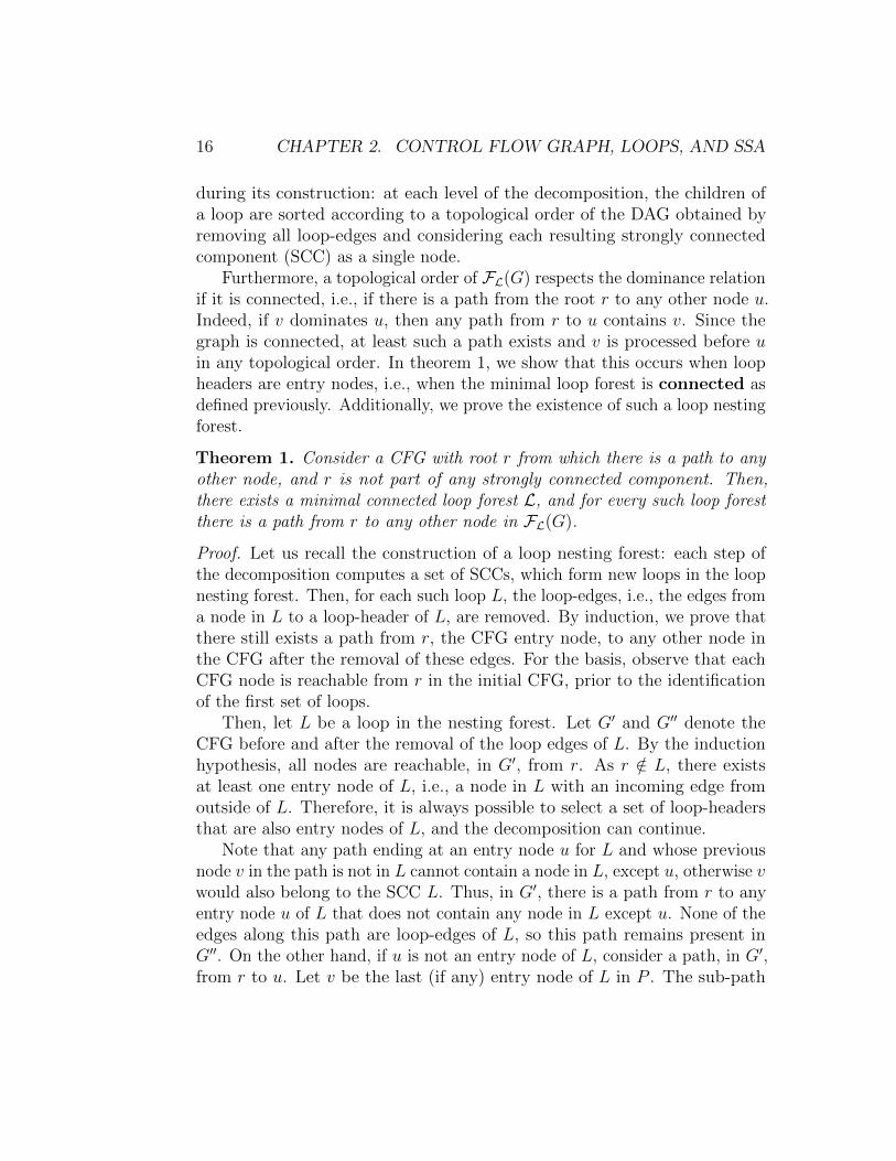
16 CHAPTER 2. CONTROL FLOW GRAPH, LOOPS, AND SSA
during its construction: at each level of the decomposition, the children ofa loop are sorted according to a topological order of the DAG obtained byremoving all loop-edges and considering each resulting strongly connectedcomponent (SCC) as a single node.
Furthermore, a topological order of FL(G) respects the dominance relationif it is connected, i.e., if there is a path from the root r to any other node u.Indeed, if v dominates u, then any path from r to u contains v. Since thegraph is connected, at least such a path exists and v is processed before uin any topological order. In theorem 1, we show that this occurs when loopheaders are entry nodes, i.e., when the minimal loop forest is connected asdefined previously. Additionally, we prove the existence of such a loop nestingforest.
Theorem 1. Consider a CFG with root r from which there is a path to anyother node, and r is not part of any strongly connected component. Then,there exists a minimal connected loop forest L, and for every such loop forestthere is a path from r to any other node in FL(G).
Proof. Let us recall the construction of a loop nesting forest: each step ofthe decomposition computes a set of SCCs, which form new loops in the loopnesting forest. Then, for each such loop L, the loop-edges, i.e., the edges froma node in L to a loop-header of L, are removed. By induction, we prove thatthere still exists a path from r, the CFG entry node, to any other node inthe CFG after the removal of these edges. For the basis, observe that eachCFG node is reachable from r in the initial CFG, prior to the identificationof the first set of loops.
Then, let L be a loop in the nesting forest. Let G′ and G′′ denote theCFG before and after the removal of the loop edges of L. By the inductionhypothesis, all nodes are reachable, in G′, from r. As r /∈ L, there existsat least one entry node of L, i.e., a node in L with an incoming edge fromoutside of L. Therefore, it is always possible to select a set of loop-headersthat are also entry nodes of L, and the decomposition can continue.
Note that any path ending at an entry node u for L and whose previousnode v in the path is not in L cannot contain a node in L, except u, otherwise vwould also belong to the SCC L. Thus, in G′, there is a path from r to anyentry node u of L that does not contain any node in L except u. None of theedges along this path are loop-edges of L, so this path remains present inG′′. On the other hand, if u is not an entry node of L, consider a path, in G′,from r to u. Let v be the last (if any) entry node of L in P . The sub-path
2.3. JOIN SET 17
from v to u does not contain any loop-edges for L and v remains reachablefrom r in G′′. Therefore, concatenating these two paths ensures that a pathfrom r to u exists in G′′.
2.3 Join set
Given a set of nodes S, let J(S) be the set of nodes x such that there existsy ∈ S, and z ∈ S, with a non-empty path from y to x and a non-empty pathfrom z to x, disjoint except for x. Let us define the iterated join set (J+(S))to be the limit of the following sequence:
J1(S) = J(S)
Ji+1(S) = J(S ∪ Ji(S))
Michael Wolfe, in [33], extended the results of Michael Weiss [32], andproved the general equivalence between the joint set and the iterated joinsets.
Theorem 2. For any set of nodes S, J(S) = J+(S).
Additionally, Cytron et al. [18] implicitly provide the following theorem onthe equivalence of join-sets and the iterated dominance frontier. An explicitversion can be found in the work of Michael Weiss [32].
Theorem 3. For any set of nodes S containing the entry, J+(S) = DF+(S).
2.4 Static single assignment (SSA) form
2.4.1 Definitions
The static single assignment (SSA) form was first presented in two papersin POPL’88, focusing on the identification and elimination of redundantcomputations [1, 12]. Those papers were followed by a journal paper [18]presenting more thoroughly the foundations of the SSA form as well as variousconstruction algorithms.
The main concept behind the SSA form is that every variable satisfiesthe single definition property. This means that every variable is only beingassigned once, textually. The property cannot be achieved with only the
18 CHAPTER 2. CONTROL FLOW GRAPH, LOOPS, AND SSA
help of renaming, that is choosing a different name for every definition of avariable and renaming every use appropriately. In some cases, two distinctdefinition reach the same use, depending on the actual execution. To solvethis issue, SSA form introduce a new concept, the φ-functions.
A φ-function can only be inserted at the start of a basic block, and isusually inserted at a join point. It has the same number of arguments asthe join point has incoming edges. Every φ-functions of a basic block areexecuted concurrently, the value returned by the function depends on theexecution flow. We suppose the incoming edges are ordered, if the instructionis reached via the i-th incoming, then the φ-function returns the value ofits i-th argument. Another way to view the operation is to imagine copieshappening on the edges, the variable at the left-hand side will have as manypotential definitions as there are incoming edges, φ-functions have the samesemantics but allow to have the single definition property.
In most cases, to simplify liveness and dominance under SSA, instead ofconsidering that the use associated with a φ-function happens on the edge,we can assume it is located at the end of the associated predecessor block.
2.4.2 Minimal SSA
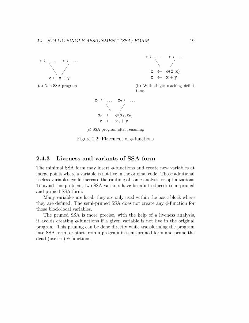
We only defined a property that must be satisfied for a program to be inSSA form and a new instruction allowing us to properly transform a programinto SSA form. We now describe how to actually transform a program intoSSA form. The textbook algorithm works in two different phases: first, thepoints where φ-functions have to be inserted are computed, then, variables arerenamed in order to satisfy the single definition property. For the placementof φ-functions, the journal paper of Cytron et al. [18] uses the notion of joinpoints: for a given variable v, φ-functions are inserted at the iterated join setJ+(D) where D is the set of program points where v is defined. It is easierto compute the iterated dominance frontier (DF+) than the join sets. SinceDF+(S) = J+(S) if S includes the root of the CFG, the algorithm fromCytron et al. adds a pseudo definition of v at the root of the control flowgraph to ensure the root node is always included in the set of definitions, thislets them use the iterated dominance frontier instead of the join sets. Afterinserting the necessary φ-functions, but before renaming the variable, wecan minimize the number of inserted φ-functions such that every use is onlyreachable from one definition, the resulting SSA form is called the minimalSSA form.
2.4. STATIC SINGLE ASSIGNMENT (SSA) FORM 19
x← . . . x← . . .
z← x + y
(a) Non-SSA program
x← . . . x← . . .
x ← φ(x, x)z ← x + y
(b) With single reaching defini-tions
x1 ← . . . x2 ← . . .
x3 ← φ(x1, x2)z ← x3 + y
(c) SSA program after renaming
Figure 2.2: Placement of φ-functions
2.4.3 Liveness and variants of SSA form
The minimal SSA form may insert φ-functions and create new variables atmerge points where a variable is not live in the original code. Those additionaluseless variables could increase the runtime of some analysis or optimizations.To avoid this problem, two SSA variants have been introduced: semi-prunedand pruned SSA form.
Many variables are local: they are only used within the basic block wherethey are defined. The semi-pruned SSA does not create any φ-function forthose block-local variables.
The pruned SSA is more precise, with the help of a liveness analysis,it avoids creating φ-functions if a given variable is not live in the originalprogram. This pruning can be done directly while transforming the programinto SSA form, or start from a program in semi-pruned form and prune thedead (useless) φ-functions.

20 CHAPTER 2. CONTROL FLOW GRAPH, LOOPS, AND SSA
Chapter 3
Liveness analysis under SSA
Liveness analysis provides information about the points in a program where avariable holds a value that might still be needed. Thus, liveness informationis necessary for most optimizations passes related to storage assignment. Forinstance optimizations like software pipelining, trace scheduling, and register-sensitive redundancy elimination make use of liveness information. In thecode generation part, particularly for register allocation, liveness informationis mandatory.
Traditionally, liveness information has been computed with data-flowanalysis techniques (e.g. see [16]). But they have major drawbacks sincethe computation is fairly expensive (several iterations are needed) and theresults are easily invalidated by program transformations. Indeed, addinginstructions or introducing new variables requires suitable changes in theliveness information: partial re-computation or degradation of its precision.Furthermore one cannot easily limit the data-flow algorithms to computeinformation only for parts of a procedure. Computing a variable’s liveness ata program location generally implies computing its liveness at other locations,too.
In this chapter we describe alternatives algorithms for computing theliveness information. We present our novel algorithm, based on the loopstructure of the graph, which builds the liveness information in two-passes:one backward in the control flow graph, and one forward in an order derivedfrom the loop structure. Then we present simpler algorithms solely basedon the exploration of paths. Finally we solve a more complex problem:interference between variables. As we will show, this problem not onlyinvolves the liveness information related to the variables, but their actual
21
22 CHAPTER 3. LIVENESS ANALYSIS UNDER SSA
value as well.
3.1 Definitions
A variable is live at some CFG node if both:
1. its value is available at this node. This can be expressed as the existenceof a reaching definition, i.e. existence of a directed path from a definitionto this node.
2. its value might be used in the future. This can be expressed as theexistence of an upward exposed use, i.e. existence of a directed pathfrom this node to a use that does not contain any definition of thisvariable.
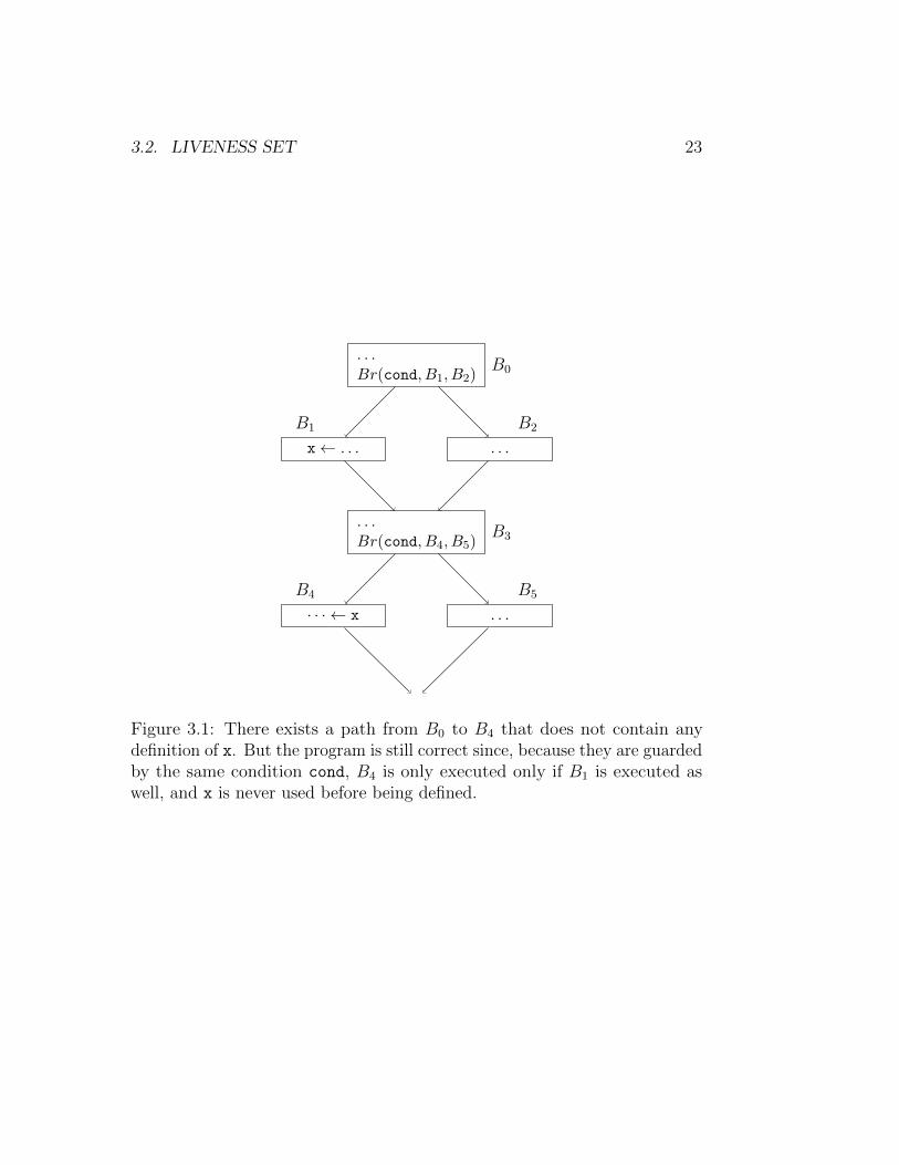
In fact, the reaching definition constraint is useful only for non-strictprograms. A strict program is a program such that every path from startnode to a use of a variable contains the definition of the variable. An upwardexposed use at the entry of the CFG, is a potential bug in the program,even if the dynamic execution could be safe, for example if every executedpath defines the variable before any use as in figure 3.1. In that case thecompiler usually dumps a warning message (use of a potentially undefinedvariable). From now on, we will assume the program to be in strict SSAform, the definition of a variable dominates all its uses (dominance property).To simplify some definitions and proofs, we sometimes consider that everyCFG node consists of a single instruction. Liveness can then be defined asfollows:
Definition 1. A variable a is live-in at a node q if there exists a directedpath from q to a node u where a is used and that path does not contain thedefinition of a, denoted as defa.
Definition 2. A variable a is live-out at a node q if it is live-in at least atone successor of q.
3.2 Liveness set
Sometimes instead of computing the program points where a variable is live,it is sufficient to compute the set of live variable only at some particular
3.2. LIVENESS SET 23
. . .Br(cond, B1, B2)
B0
x← . . .
B1
. . .
B2
. . .Br(cond, B4, B5)
B3
· · · ← x
B4
. . .
B5
Figure 3.1: There exists a path from B0 to B4 that does not contain anydefinition of x. But the program is still correct since, because they are guardedby the same condition cond, B4 is only executed only if B1 is executed aswell, and x is never used before being defined.
24 CHAPTER 3. LIVENESS ANALYSIS UNDER SSA
program point. Typically, live sets are computed at basic blocks boundaries,since the lack of control flow inside basic blocks allows to recompute theprecise liveness information easily. We call this analysis the computation oflive-in and live-out sets.
3.2.1 Classical liveness set construction
We defined liveness in term of the existence of paths, that is a relation betweena node and its successors. Since liveness information evolves around paths,the traditional approach has been to describe the problem using data-flowequations. Indeed, the live-in and live-out definitions are easily mapped intoa set of data-flow equations.
We assume we are under strict SSA Form, thus every variable has a uniquedefinition which dominates all its uses. Let us note Killing(B) the set ofvariables which are defined in the basic block B, and UpwardExposed(B) theset of variable that are used in the basic block and are defined in another basicblock. Intuitively, we consider a basic block as a huge instruction, definingsome variables (Killing) and using other variables (UpwardExposed), whileany local variable that does not escape the basic block is omitted. We canthen simply map the definitions to the following equations:
LiveIn(B) = UpwardExposed(B) ∪ (LiveOut(B)−Killing(B))
LiveOut(B) = ∪S∈succs(B)LiveIn(S)
Those equations translate to the data-flow algorithm found in algorithm 3.
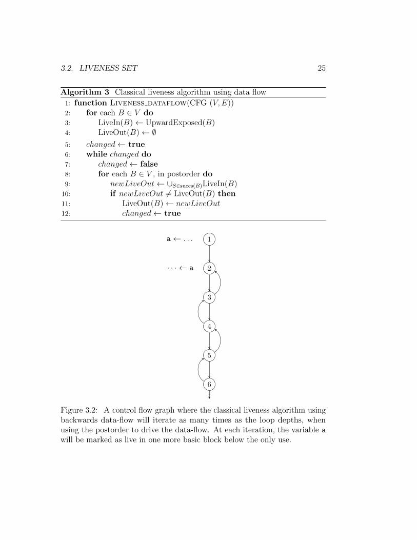
As with all data-flow analysis, the order in which the CFG nodes areprocessed is crucial. If the graph was acyclic, ordering the nodes such thatevery node is processed after all its successors are processed would avoiddoing any iteration. An example of such an order is the postorder of a graph.In practice even if most control flow graphs have loops, thus the postorderwill not make the information flow everywhere in one pass, but it will stillpropagate quite far, that is the reason why the chosen order is usually thepostorder.
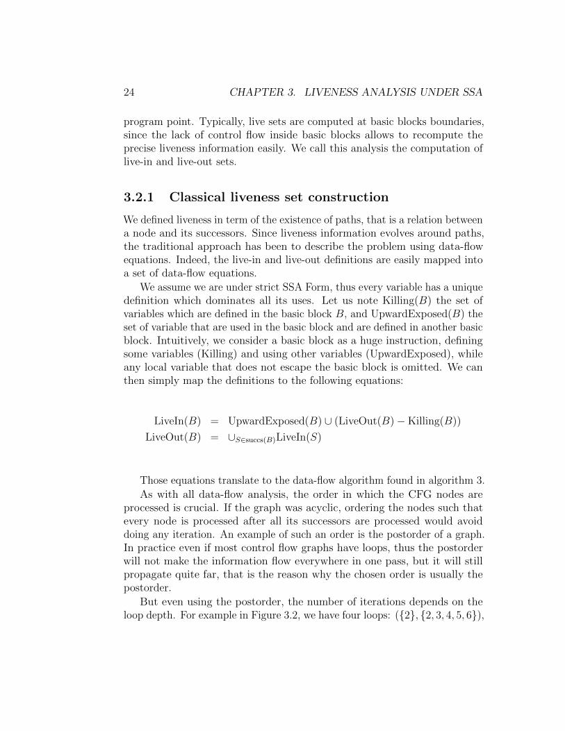
But even using the postorder, the number of iterations depends on theloop depth. For example in Figure 3.2, we have four loops: ({2}, {2, 3, 4, 5, 6}),
3.2. LIVENESS SET 25
Algorithm 3 Classical liveness algorithm using data flow
1: function Liveness dataflow(CFG (V,E))2: for each B ∈ V do3: LiveIn(B)← UpwardExposed(B)4: LiveOut(B)← ∅5: changed← true6: while changed do7: changed← false8: for each B ∈ V , in postorder do9: newLiveOut← ∪S∈succs(B)LiveIn(B)
10: if newLiveOut 6= LiveOut(B) then11: LiveOut(B)← newLiveOut12: changed← true
1a← . . .
2· · · ← a
3
4
5
6
Figure 3.2: A control flow graph where the classical liveness algorithm usingbackwards data-flow will iterate as many times as the loop depths, whenusing the postorder to drive the data-flow. At each iteration, the variable a
will be marked as live in one more basic block below the only use.
26 CHAPTER 3. LIVENESS ANALYSIS UNDER SSA
({3}, {3, 4, 5, 6}), ({4}, {4, 5, 6}) and ({5}, {5, 6}). After each iteration, theinformation will reach one more loop starting from the outermost one.
We can note that, in the case of forward data-flow, Cooper [17] advocatefor the use of a reverse postorder of the control flow graph. For backward-dataflow algorithm, most authors [3] simply assume it is the same type of problemswith the edges reversed and thus use the reverse postorder of the control flowgraph with all edges reversed. But we do not see any compelling reason tochoose this order over a simpler postorder of the control flow graph.
Kam et al. [24] explored the complexity of round-robin data-flow algo-rithms, that is algorithms that iterate over a fixed order until there are nonew changes. They show that for forward data-flow problems, if the graph isreducible, there will be at most d(G) + 3 passes over the set of nodes, whered(G) is the depth of the most nested loop. To apply this complexity analysisto backwards data-flow problems, the reverse control flow graph needs tobe reducible. However while most control flow graph are reducible, it is nottrue from a typical reverse control flow graph: many programming languagesoffer a way to break out of a loop from multiple locations. Furthermore somecompiler have passes to transform every loop of a control flow graph intoa natural loop, but those passes are usually not applicable for the reversecontrol flow graph. It is an open conjecture to know if the bound provedby Kam et al. [24] is valid for backwards data-flow with postorder. If thatconjecture was proven, it would remove any incentive to use the reversepostorder of the reverse graph for round-robin algorithms solving backwarddata-flow problems.
3.2.2 Two pass data flow
As we have seen with the classical data-flow algorithm, the algorithm needsto iterate in order to propagate the information across loops. With the helpof SSA properties, and using the loop structure, can we do better?
The use of SSA properties, single definition and dominance, allows tocompute the liveness information in two passes. We show the result first forreducible graphs, and will generalize to non-reducible graphs later on. First,a backward pass propagates the liveness information upwards to the loopheaders. Then a second pass propagates the liveness from the header of theloops to their bodies.
The first past consists on a propagation of the liveness, in a way similar toa single pass of a round-robin data-flow algorithm, using a reverse topological
3.2. LIVENESS SET 27
order of the acyclic graph where the loop-edges are removed (the reducedgraph, FL(G)). The second pass descends into the loop tree, propagating theliveness from headers to the loop body for each loop.
We first show that the backward pass on a reverse topological order ofthe reduced graph correctly propagates the information to the loop headers.
Lemma 1. In a reducible CFG, given a variable v and its definition d, forevery maximal loop L with header h such that L does not contain d, v islive-in at h iff there is a path in FL(G), the reduced graph, from h to a usenot containing d.
Proof. Given a variable v defined in d, and a maximal loop L with headerh not containing d. If v is live at h, there exists a cycle-free path from h toa use of v in the CFG, which does not go through d. Take this path andsuppose there is a loop-edge (s, h′) in this path, h′ being the header of a loopL′, and s ∈ L′. h′ 6= h otherwise the path would contain a cycle, this meansL 6= L′.
• h ∈ L′ is not possible, since L was the biggest loop not containing d, itwould imply d ∈ L′ and h would dominate d which contradicts the factthat v is live-in at h.
• h 6∈ L′, since the graph is reducible, the only way to enter L′ is throughh′, and it would mean there was a previous occurrence of h′ in the path,this breaks our hypothesis that the path is cycle-free.
Thus the path does not contain any loop-edges, and it is a valid path fromthe acyclic graph. Conversely, if there exists a path in the acyclic graph, thenv is live-in at h, since the acyclic graph is a subgraph of the CFG.
In the previous lemma, it is not guaranteed there exists a loop L satisfyingthe conditions. The following lemma covers this case:
Lemma 2. In a reducible CFG, given a variable v and its definition d, forevery program point p such that no loop contains p but not d, v is live-in at piff there is a path in the reduced graph FL(G) from p to a use not containingd.
Proof. Given a variable v defined in d, and a program point p such that v islive at p and no loop contains p but not d. Since v is live at p, there exists acycle-free path from p to a use of v in the CFG, that does not go through d.
28 CHAPTER 3. LIVENESS ANALYSIS UNDER SSA
Take this path and suppose there is a loop-edge (s, h) in this path, h beingthe header of a loop L, and s ∈ L:
• p ∈ L is not possible, since it would imply d ∈ L and h would dominated.
• p 6∈ L, since the graph is reducible, the only way to enter L is throughh, and it would mean there was a previous occurrence of h in the path,this breaks our hypothesis that the path is cycle-free.
We built a path which does not contain any loop-edges, thus a valid pathfrom the acyclic graph. Conversely, if there exists a path in the acyclic graph,then v is live-in at p, since the acyclic graph is a subgraph of the CFG.
Those two lemmas prove that if we propagate the liveness informationonly along the edges of FL(G), the acyclic reduced graph, then for a variablev, every program point that is either not part of a loop not containing d, or isthe header of the biggest loop not containing d, will have v marked as live-in.
Furthermore, the first lemma proves that if after the first pass (thebackwards propagation along the reduced graph) a program point’s live-inis not accurate, then the missing variable is already in the live-in set of theheader of one of the surrounding loops. We now prove that every variablelive-in at the header of the loop should also be live-in at every program pointof the loop body.
Lemma 3. If a variable v is live-in at a header of a loop, then v is live-in ateach node from the body of the loop,
Proof. Given a loop L with header h, such that the variable v defined atd is live-in at the loop (it is live-in at h). Since it is live at h, because ofthe dominance property, h is strictly dominated by d, this mean d is notcontained in L. Furthermore there exists a path from h to a use of v whichdoes not go through d. For every node of the loop, p, since the loop is astrongly connected component of the CFG, there exists a path, consistingonly of nodes from L from p to h. Concatenating those two paths proves thatv is live-in and live-out of p.
This lemma proves the correctness of the second pass, which propagatesthe liveness information inside loops. Lemma 1 proved that every programpoint which did not have a correct liveness information will be marked after
3.2. LIVENESS SET 29
the second pass, this lemma proves that every program point marked by thepass is indeed live-in. Overall, this proves the correctness of our algorithm.
While a round-robin data-flow algorithm can, in the worst-case, do asmany iteration as the depth of the loop nesting forest, with our loop-basedalgorithm, the first pass will update the header of the outermost loop, whilethe second pass will directly update every node part of the loop, includingthe bottom. No iteration is needed. That is the case in Figure 3.2: the firstpass will update the liveness information for the outermost loop header (2),and the second pass will update all its descendants in the loop-nesting forest(3, 4, 5, 6).
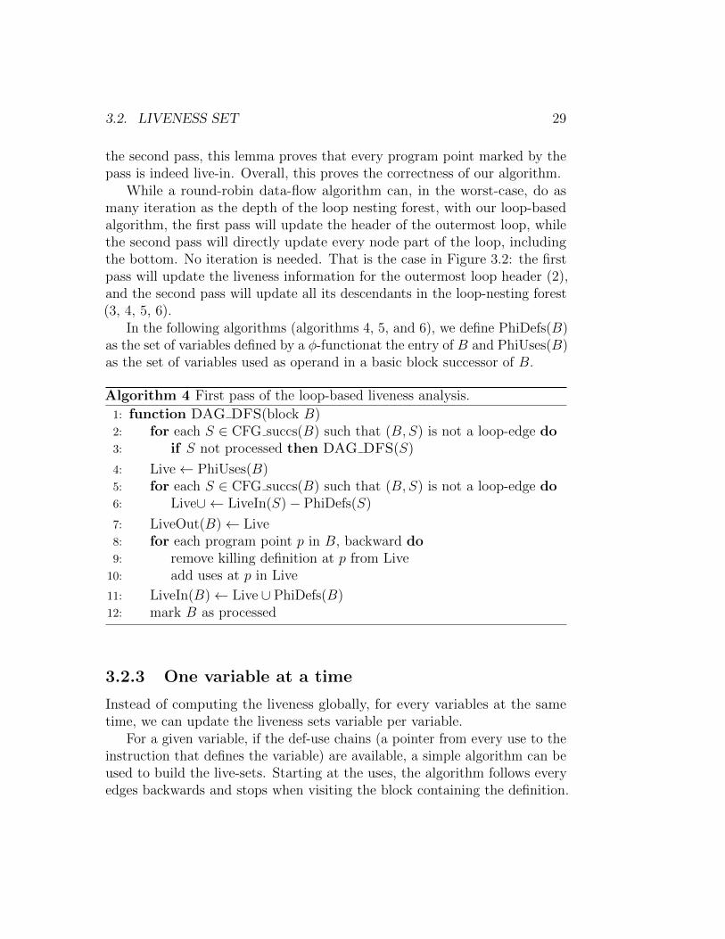
In the following algorithms (algorithms 4, 5, and 6), we define PhiDefs(B)as the set of variables defined by a φ-functionat the entry of B and PhiUses(B)as the set of variables used as operand in a basic block successor of B.
Algorithm 4 First pass of the loop-based liveness analysis.
1: function DAG DFS(block B)2: for each S ∈ CFG succs(B) such that (B, S) is not a loop-edge do3: if S not processed then DAG DFS(S)
4: Live← PhiUses(B)5: for each S ∈ CFG succs(B) such that (B, S) is not a loop-edge do6: Live∪ ← LiveIn(S)− PhiDefs(S)
7: LiveOut(B)← Live8: for each program point p in B, backward do9: remove killing definition at p from Live
10: add uses at p in Live
11: LiveIn(B)← Live ∪ PhiDefs(B)12: mark B as processed
3.2.3 One variable at a time
Instead of computing the liveness globally, for every variables at the sametime, we can update the liveness sets variable per variable.
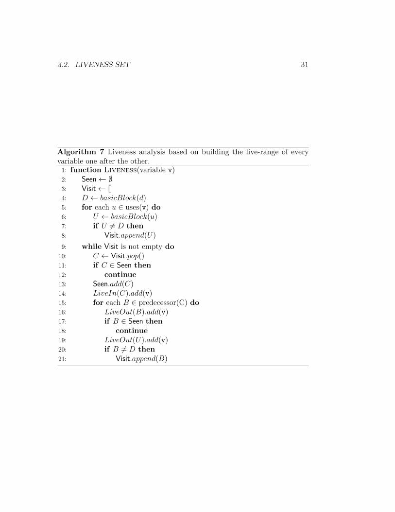
For a given variable, if the def-use chains (a pointer from every use to theinstruction that defines the variable) are available, a simple algorithm can beused to build the live-sets. Starting at the uses, the algorithm follows everyedges backwards and stops when visiting the block containing the definition.
30 CHAPTER 3. LIVENESS ANALYSIS UNDER SSA
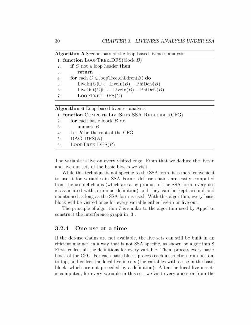
Algorithm 5 Second pass of the loop-based liveness analysis.
1: function LoopTree DFS(block B)2: if C not a loop header then3: return4: for each C ∈ loopTree children(B) do5: LiveIn(C)∪ ← LiveIn(B)− PhiDefs(B)6: LiveOut(C)∪ ← LiveIn(B)− PhiDefs(B)7: LoopTree DFS(C)
Algorithm 6 Loop-based liveness analysis
1: function Compute LiveSets SSA Reducible(CFG)2: for each basic block B do3: unmark B4: Let R be the root of the CFG5: DAG DFS(R)6: LoopTree DFS(R)
The variable is live on every visited edge. From that we deduce the live-inand live-out sets of the basic blocks we visit.
While this technique is not specific to the SSA form, it is more convenientto use it for variables in SSA Form: def-use chains are easily computedfrom the use-def chains (which are a by-product of the SSA form, every useis associated with a unique definition) and they can be kept around andmaintained as long as the SSA form is used. With this algorithm, every basicblock will be visited once for every variable either live-in or live-out.
The principle of algorithm 7 is similar to the algorithm used by Appel toconstruct the interference graph in [3].
3.2.4 One use at a time
If the def-use chains are not available, the live sets can still be built in anefficient manner, in a way that is not SSA specific, as shown by algorithm 8.First, collect all the definitions for every variable. Then, process every basic-block of the CFG. For each basic block, process each instruction from bottomto top, and collect the local live-in sets (the variables with a use in the basicblock, which are not preceded by a definition). After the local live-in setsis computed, for every variable in this set, we visit every ancestor from the
3.2. LIVENESS SET 31
Algorithm 7 Liveness analysis based on building the live-range of everyvariable one after the other.
1: function Liveness(variable v)2: Seen← ∅3: Visit← []4: D ← basicBlock(d)5: for each u ∈ uses(v) do6: U ← basicBlock(u)7: if U 6= D then8: Visit.append(U)
9: while Visit is not empty do10: C ← Visit.pop()11: if C ∈ Seen then12: continue13: Seen.add(C)14: LiveIn(C).add(v)15: for each B ∈ predecessor(C) do16: LiveOut(B).add(v)17: if B ∈ Seen then18: continue19: LiveOut(U).add(v)20: if B 6= D then21: Visit.append(B)
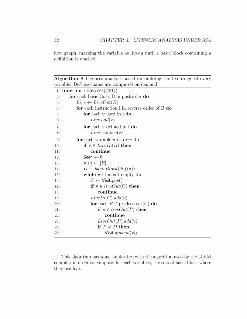
32 CHAPTER 3. LIVENESS ANALYSIS UNDER SSA
flow graph, marking the variable as live-in until a basic block containing adefinition is reached.
Algorithm 8 Liveness analysis based on building the live-range of everyvariable. Def-use chains are computed on demand.
1: function Liveness(CFG)2: for each basicBlock B in postorder do3: Live← LiveOut(B)4: for each instruction i in reverse order of B do5: for each v used in i do6: Live.add(v)
7: for each v defined in i do8: Live.remove(v)
9: for each variable v in Live do10: if v ∈ LiveIn(B) then11: continue12: Seen← ∅13: Visit← [B]14: D ← basicBlock(def(v))15: while Visit is not empty do16: C ← Visit.pop()17: if v ∈ liveOut(C) then18: continue19: LiveIn(C).add(v)20: for each P ∈ predecessor(C) do21: if v ∈ liveOut(P ) then22: continue23: LiveOut(P ).add(v)24: if P 6= D then25: Visit.append(B)
This algorithm has some similarities with the algorithm used by the LLVMcompiler in order to compute, for each variables, the sets of basic block wherethey are live.
3.3. LIVENESS CHECK 33
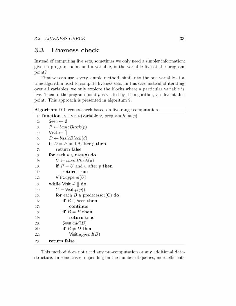
3.3 Liveness check
Instead of computing live sets, sometimes we only need a simpler information:given a program point and a variable, is the variable live at the programpoint?
First we can use a very simple method, similar to the one variable at atime algorithm used to compute liveness sets. In this case instead of iteratingover all variables, we only explore the blocks where a particular variable islive. Then, if the program point p is visited by the algorithm, v is live at thispoint. This approach is presented in algorithm 9.
Algorithm 9 Liveness-check based on live-range computation.
1: function IsLiveIn(variable v, programPoint p)2: Seen← ∅3: P ← basicBlock(p)4: Visit← []5: D ← basicBlock(d)6: if D = P and d after p then7: return false8: for each u ∈ uses(v) do9: U ← basicBlock(u)
10: if P = U and u after p then11: return true12: Visit.append(U)
13: while Visit 6= [] do14: C = Visit.pop()15: for each B ∈ predecessor(C) do16: if B ∈ Seen then17: continue18: if B = P then19: return true20: Seen.add(B)21: if B 6= D then22: Visit.append(B)
23: return false
This method does not need any pre-computation or any additional data-structure. In some cases, depending on the number of queries, more efficients
34 CHAPTER 3. LIVENESS ANALYSIS UNDER SSA
methods can be used. If we pre-compute some data-structures first, the querycost can be lowered.
We now describe such a solution, where we use an auxiliary data structureto lower the query cost. First we examine the case where the graph is reducible.We will later adapt our algorithm to the more general case of potentiallyirreducible graphs.
Using the results from 3.2.2, we know that a variable defined at a programpoint d is live at a program point p iff it is live at p or at the header of thebiggest loop containing p and not d, using only FL(G), the acyclic reducedgraph, to test for reachability.
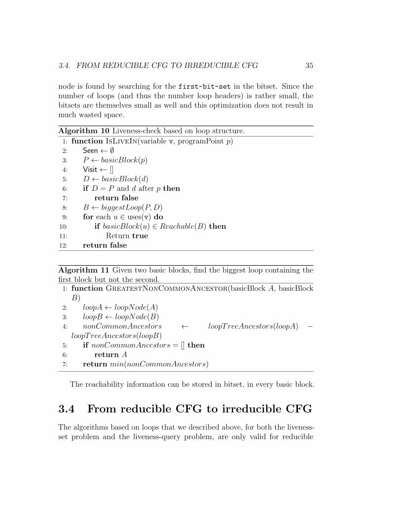
Given the reduced graph and the loop nesting forest, finding out if avariable is live at some program point can be done in two steps, as shownin algorithm 10. First, if there exists a loop containing the program point pand not the definition, pick the header of the biggest such loop instead asthe query point. Then check for reachability from this program point to anyuse of the variable. Correctness is proved from the theorems used for livenesssets.
Finding the biggest loop not containing the definition but containing thequery point is a problem similar to finding the least common ancestor (LCA)of two nodes in a tree: the loop in question is the only direct child of the leastcommon ancestor which is an ancestor of the smallest loop containing thequery point. A LCA query can be answered in O(1), with a pre-computationof O(n), as described in [4]. The algorithm described by Bender is based onthe Euler tour of the tree, that is the sequence of nodes as they are visitedby a depth first search. A simple adaptation of their algorithm can be made,based on the insight that the biggest loop containing the query but not thedefinition is the next node after the last occurrence of the LCA in an Eulertour of the loop-tree.
But since the depth of the tree is usually small, a simpler solution can beused: the naive solution that just walks upward in the tree starting at bothnodes and stops when it encounter a common ancestor.
The third alternative method (shown in algorithm 11) is to pre-computethe set of ancestors from the loop-tree for every node. Then a simple setoperation can find the node we are looking for: the ancestor of the definitionnode are removed from the ancestor of the query point. From the remainingancestors, we pick the shallowest. Using bitsets, indexed with a topologicalorder of the loop tree, this operations are easily implemented. The removal isa bit-inversion followed by a bitwise-and operation, and the shallowest
3.4. FROM REDUCIBLE CFG TO IRREDUCIBLE CFG 35
node is found by searching for the first-bit-set in the bitset. Since thenumber of loops (and thus the number loop headers) is rather small, thebitsets are themselves small as well and this optimization does not result inmuch wasted space.
Algorithm 10 Liveness-check based on loop structure.
1: function IsLiveIn(variable v, programPoint p)2: Seen← ∅3: P ← basicBlock(p)4: Visit← []5: D ← basicBlock(d)6: if D = P and d after p then7: return false8: B ← biggestLoop(P,D)9: for each u ∈ uses(v) do
10: if basicBlock(u) ∈ Reachable(B) then11: Return true12: return false
Algorithm 11 Given two basic blocks, find the biggest loop containing thefirst block but not the second.
1: function GreatestNonCommonAncestor(basicBlock A, basicBlockB)
2: loopA← loopNode(A)3: loopB ← loopNode(B)4: nonCommonAncestors ← loopTreeAncestors(loopA) −loopTreeAncestors(loopB)
5: if nonCommonAncestors = [] then6: return A7: return min(nonCommonAncestors)
The reachability information can be stored in bitset, in every basic block.
3.4 From reducible CFG to irreducible CFG
The algorithms based on loops that we described above, for both the liveness-set problem and the liveness-query problem, are only valid for reducible
36 CHAPTER 3. LIVENESS ANALYSIS UNDER SSA
graphs. We can derive an algorithm that works for irreducible graphs as well,in the following way: transform the irreducible graph to a reducible graphwhile keeping the liveness identical, in practice the graph is not actuallymodified, but the algorithms are changed to simulate the modification of someedges, on the fly.
As hinted by Ramalingam, adding a dummy node to represent the headerscan help dealing with irreducible graphs. Contrary to Ramalingam we wantto keep the liveness identical as well, not only the dominance information.
We can iteratively construct our modified graph G′ from the control flowgraph G in the following way:
Given a loop L, we define a new graph Ψ′L as (V ′, E ′), where:
V ′ = V ∪ {δL}E ′ = E − LoopEdges(L)− EntryEdges(L)
∪{(p, δL)|p ∈ PreEntries(L)}∪{(p, δL)|∃x ∈ Headers(L), (p, x) ∈ LoopEdges(L)}∪{(δL, h)|h ∈ Entries(L) ∪ Headers(L)}
In other words, for a given loop L, add a new node to the graph: δL.Replace every entry 1 edge (x, y) by two edges (x, δL) and (δL, y). Similarlyreplace every loop-edge (x, y) by two edges (x, δL) and (δL, y).
Applying the transformation to every loop in the forest, will transform Ginto G′. Contrary to the graph built by Ramalingam, G′ is not acyclic. In factthe loop structure is preserved. Furthermore, since, from the construction,every loop has only one entry node (δL), the graph is reducible.
Theorem 4. Given a loop L, for every two nodes x and y from G, x dom yin G iff x dom y in Ψ′L.
Proof. Take two nodes x and y from G, such that x dom y in Ψ′L. Givenp an arbitrary path in G from r to y, we show that x is included in thatpath. From p, we construct p′ a path in Ψ′L from r to y as follow: for everyedge (u, v) from p not present in Ψ′L (v is a header or an entry node), (u, δL)and (δL, v) are valid edges from E ′, and we replace (u, v) by those two edges.Since x dom y in Ψ′L, and p′ is a path from r to y, it must include x. δL is
1it is important not to restrict to the loop headers
3.4. FROM REDUCIBLE CFG TO IRREDUCIBLE CFG 37
the only node in p′ that was not in the original path p, this proves x was inthe original path.
Reciprocally, suppose that x dom y in G. We show that any path fromΨ′L, p, from r to y, goes through x. We construct a path in G using p as abasis. Starting from the end of the path, for every sub-path u, δL, v in p:
• if x ∈ L, then there exists a path, p′, from r to v in G which might onlycontain x as the last node (v is not dominated by any other node fromthe body of L), we replace the sub-path from r to v with p′ and stopthe transformation.
• else x 6∈ L, then there exists v′ ∈ L such that (u, v′) ∈ E and there isa path in G included in L from v′ to v, this path does not contain x(x 6∈ L) and the sub-path can be replaced by the path from L.
Finally we have a path in G, from r to y. Because x dom y, this pathcontains x. Since our transformation did not add x, x was in p.
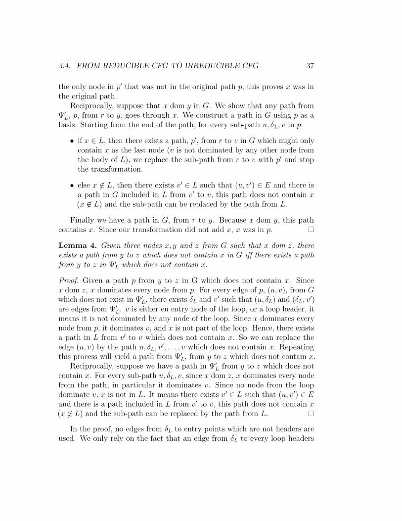
Lemma 4. Given three nodes x, y and z from G such that x dom z, thereexists a path from y to z which does not contain x in G iff there exists a pathfrom y to z in Ψ′L which does not contain x.
Proof. Given a path p from y to z in G which does not contain x. Sincex dom z, x dominates every node from p. For every edge of p, (u, v), from Gwhich does not exist in Ψ′L, there exists δL and v′ such that (u, δL) and (δL, v
′)are edges from Ψ′L. v is either en entry node of the loop, or a loop header, itmeans it is not dominated by any node of the loop. Since x dominates everynode from p, it dominates v, and x is not part of the loop. Hence, there existsa path in L from v′ to v which does not contain x. So we can replace theedge (u, v) by the path u, δL, v
′, . . . , v which does not contain x. Repeatingthis process will yield a path from Ψ′L, from y to z which does not contain x.
Reciprocally, suppose we have a path in Ψ′L from y to z which does notcontain x. For every sub-path u, δL, v, since x dom z, x dominates every nodefrom the path, in particular it dominates v. Since no node from the loopdominate v, x is not in L. It means there exists v′ ∈ L such that (u, v′) ∈ Eand there is a path included in L from v′ to v, this path does not contain x(x 6∈ L) and the sub-path can be replaced by the path from L.
In the proof, no edges from δL to entry points which are not headers areused. We only rely on the fact that an edge from δL to every loop headers
38 CHAPTER 3. LIVENESS ANALYSIS UNDER SSA
exists. This will allow us to omit those edges in the following algorithms. Itmeans that while omitting them affects the equivalence for dominance, theydo not play any role for the liveness analysis.
Theorem 5. For any SSA variable, and a node from G, it is live in G iff itis live in Ψ′L.
Proof. Direct from the existence of the path in previous lemma.
With this equivalence, we use the transformation of the control flow graphto use our previous algorithm with irreducible graphs. The simplest solutionis to build the transformed graph, adding the necessary new edges, removingothers and adding new nodes for every loop (δL nodes). But we would like toemphasize that actually modifying the graph is not required.
The modification is quite simple in practice, and even more if we restrictourself to loop-forest which only have one header per loop (as is the case ofthe loop forest structure presented by Havlak [21]) In this case, we do notneed to insert any δL nodes. The header node and δL can be merged, sinceδL has only one outgoing edge, and the header has only one incoming edge.
Additionally, the insertion and removal of edges can be simulated as well:we need to redirect any entry- or loop- edge to it’s δL node. We virtualizethe modification of the CFG in the following way: for every visited edge, ifthe target of the edge is not part of the same loop, we virtually replace theedge by an edge to the δL node of the biggest loop containing the target butnot the source of the edge. We would then need to add an edge from the δLnode to every entry or header node. But as shown in our proof for livenessequivalence, the edges to the entry nodes are not necessary.
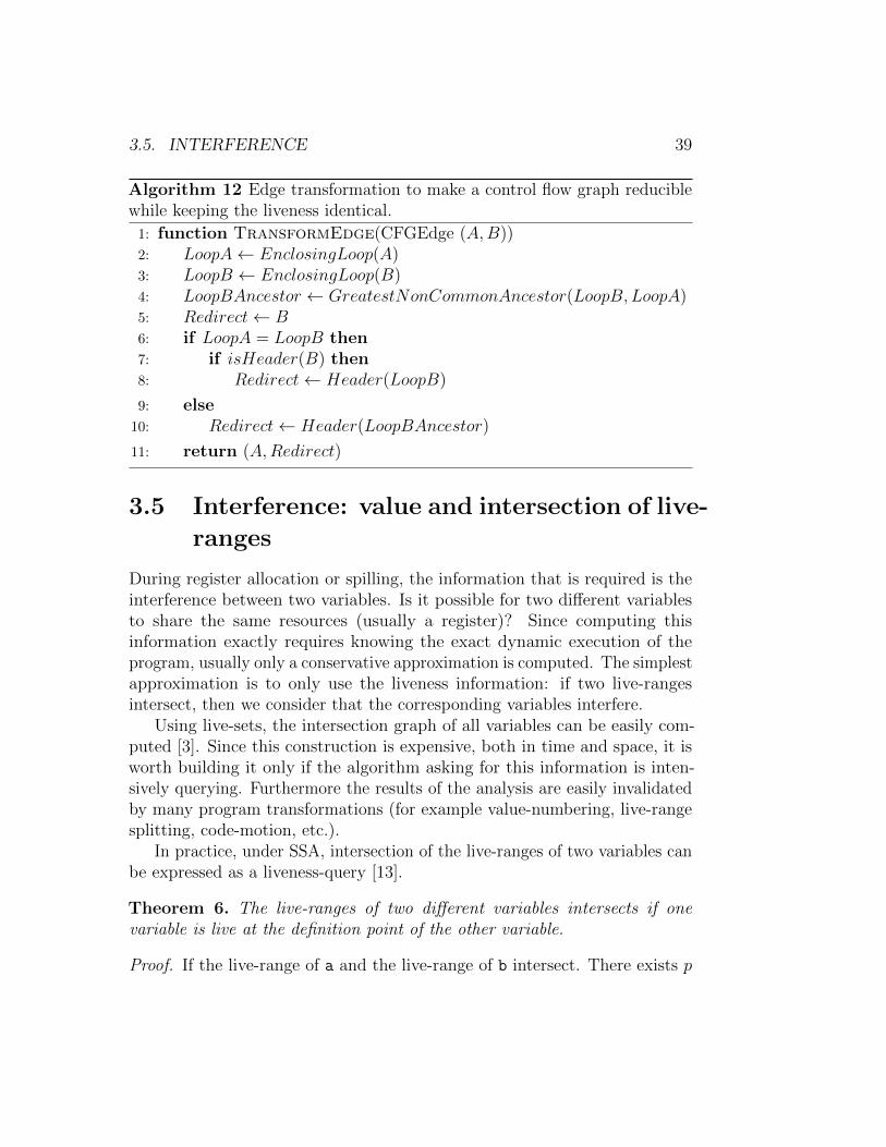
To summarize, if our loop forest only have one header per loop, thetransformation is extremely simple, during the graph traversal, every entryedge is simply redirected to the header of the biggest loop containing thetarget but not the source (see algorithm 12). This transformation needs tobe done for the computation of the reachable set, and for the DAG DFSpass for liveness set, in both cases, every edge in CFG succs needs to betransformed before further processing.
3.5. INTERFERENCE 39
Algorithm 12 Edge transformation to make a control flow graph reduciblewhile keeping the liveness identical.
1: function TransformEdge(CFGEdge (A,B))2: LoopA← EnclosingLoop(A)3: LoopB ← EnclosingLoop(B)4: LoopBAncestor ← GreatestNonCommonAncestor(LoopB,LoopA)5: Redirect← B6: if LoopA = LoopB then7: if isHeader(B) then8: Redirect← Header(LoopB)
9: else10: Redirect← Header(LoopBAncestor)
11: return (A,Redirect)
3.5 Interference: value and intersection of live-
ranges
During register allocation or spilling, the information that is required is theinterference between two variables. Is it possible for two different variablesto share the same resources (usually a register)? Since computing thisinformation exactly requires knowing the exact dynamic execution of theprogram, usually only a conservative approximation is computed. The simplestapproximation is to only use the liveness information: if two live-rangesintersect, then we consider that the corresponding variables interfere.
Using live-sets, the intersection graph of all variables can be easily com-puted [3]. Since this construction is expensive, both in time and space, it isworth building it only if the algorithm asking for this information is inten-sively querying. Furthermore the results of the analysis are easily invalidatedby many program transformations (for example value-numbering, live-rangesplitting, code-motion, etc.).
In practice, under SSA, intersection of the live-ranges of two variables canbe expressed as a liveness-query [13].
Theorem 6. The live-ranges of two different variables intersects if onevariable is live at the definition point of the other variable.
Proof. If the live-range of a and the live-range of b intersect. There exists p
40 CHAPTER 3. LIVENESS ANALYSIS UNDER SSA
a program point where a is live and b is live. Since the variables are underSSA Form, the definitions of a and b dominates p. We know that defa dom pand defb dom p, so one if the definition must dominate the other. Supposedefa dom defb.
So there is a path, from defb to p, which does not contain defa. Since a islive at p, there is a path from p to a use of a which does not contains defa.This proves that a is live at defb.
Instead of building the intersection graph of the variables, we can dynam-ically answer intersection queries using the liveness-query algorithm shown inthe previous section. Since the pre-computation only relies on the shape ofthe CFG, not on the variables themselves, no updates are necessary when anew variable is introduced.
It is common to find in the literature the following definition of interference“two variables interfere if their live ranges intersect” (e.g. in [20, 13, 30]) orits refinement “two variables interfere if one is live at a definition point of theother” (e.g. in [14]). Actually, a and b interfere only if they cannot be storedin a common register. Chaitin et al. discuss more precisely an “ultimatenotion of interference” [15]: a and b cannot be stored in a common registerif there exists an execution point where a and b carry two different valuesthat are both defined, used in the future, and not redefined between theirdefinition and use.
This definition of interference contains two dynamic (i.e., related to theexecution) notions: the notion of liveness and the notion of value. Analyzingstatically if a variable is live at a given execution point is not decidable sinceit can be reduced to the halting problem (given a variable defined at the entryof the program and only used at the exit node, it is live at the exit node if andonly if the program terminates). We previously provided a (quite accurate inpractice) approximation defined with paths: reaching definition and upwardexposed use [3]. In SSA with the dominance property – in which each useis dominated by its unique definition, so it is defined – upward exposed useanalysis is sufficient.
The notion of value is even harder and can be approximated using dataflow analysis on non trivial lattices (see for example [1, 7]). This has beenextensively studied in particular in the context of partial redundancy elimi-nation. The scope of variable coalescing is usually not so large, and Chaitinproposed the following conservative test: two variables interfere if one is liveat a definition point of the other and this definition is not a copy between
3.5. INTERFERENCE 41
the two variables.
This interference notion is the most commonly used, see for example howthe interference graph is computed in [3].
Chaitin et al. noticed that, with this conservative interference definition,when a and b are coalesced, the set of interferences of the new variablemay be strictly smaller than the union of interferences of a and b. Thus,simply merging the two corresponding nodes in the interference graph is anover-approximation with respect to the interference definition.
For example, in a block with two successive copies b← a and c← a wherea is defined before, and b and c (and possibly a) used after, it is consideredthat b and c interfere but that none of them interfere with a. However, aftercoalescing a and b, c should not interfere anymore with the coalesced variable.
Hence, the interference graph has to be updated or rebuilt. Chaitin etal. [15] proposed a counting mechanism, rediscovered in [19], to update the in-terference graph, but it was considered as too space consuming. Recomputingit from time to time was preferred [15, 14]. Since then, most coalescing tech-niques based on graph coloring use either live-range intersection graph [31, 13]or Chaitin’s interference graph with reconstructions [20, 11].
Actually, in SSA with the dominance property, things are simpler. Eachvariable has, statically, a unique value, given by its unique definition. Fur-thermore, the “has-the-same-value” binary relation defined on variables isan equivalence relation. This property is used in SSA dominance-based copyfolding or global value numbering [10]. The value of an equivalence class isthe variable whose definition dominates the definitions of all other variablesin the class.
Hence, using the same scheme as SSA copy folding or constant propagation,finding the value of a variable can be done by a simple topological traversalof the dominance tree: when reaching an assignment of a variable b, if theoperation is a copy b← a, V (b) is set to V (a), otherwise V (b) is set to b.
The interference test is now both simple and accurate (no need to re-build/update after a coalescing): a interfere with b if live(a) intersects live(b)and V (a) 6= V (b). (The first part reduces to def(a) ∈ live(b) or def(b) ∈ live(a)thanks to the dominance property [13].)
42 CHAPTER 3. LIVENESS ANALYSIS UNDER SSA
3.6 Conclusion
In this chapter we have presented three contributions, based on propertiesbrought by the SSA form. First we described our novel liveness algorithm,which constructs live-sets for each basic block based on the structure of theloops. The more classical liveness algorithm, based on a data-flow approach,visits every edge and iterates multiple times until no further change appears.On the contrary, our algorithm first visits every edge once, and then visitsevery node a second time.
Then, based on the insight that many modifications of the code invalidatesthe liveness-sets, we propose an alternative approach: the liveness checking.Instead of building the set of live variables, we pre-compute some datastructure, and only answer to the question “is the variable live at this programpoint?”. The precomputed data structure only depends on the shape of thecontrol flow graph, this means that most modifications of the code (insertingnew instructions for example) will not invalidate the data.
Finally, liveness is often used to compute the interference between variables.But interference does not consist of checking if the live-ranges intersect, it alsodepends if the variables hold the same value. Chaitin gave an ultimate notionof interference, and provided an approximation. We give an algorithm whichprovides a more precise approximation and which does not need complexupdates when the code changes.
Chapter 4
SSA extensions: SSI
Since the inception of the SSA form, many variants have been presented,usually in order to facilitate some analysis. In this chapter we present one ofthis variant the Static Single Information (SSI) form. Different definitions haveappeared in the literature since it was first introduced. Our first contribution isto clarify the differences between those definitions. Then we prove a propertyrelated to liveness and the SSI form: the intersection graph of variables underSSI (the intersection of the live-range of the variables) is an interval graph.This allows us to build liveness algorithms which make use of this property.
4.1 Definitions and motivations
The static single information (SSI) form is an extension of SSA formthat treats uses and definitions symmetrically with respect to one another.We now explore the different definitions found in the literature, by Ananianand by Singer.
4.1.1 Ananian’s definition of SSI
Ananian introduced the SSI form in a similar way as Cytron et al. did forSSA, i.e., using properties on paths [2]. For this purpose, we use the notionsof split set (similar to join set for SSA) and of upward-exposed use (similarto reaching definition for SSA).
The split set of two CFG nodes u 6= v, denoted S({u, v}), is the set ofnodes w such that there exist two paths, one from w to u and one from w to
43
44 CHAPTER 4. SSA EXTENSIONS: SSI
v, with only w in common. A use of a variable x is upward-exposed at aprogram point p if there is a path from p to the use that does not go throughany other use of x. 1 A procedure satisfies the single upward-exposed-useproperty if at most one use of each variable is upward-exposed at eachprogram point p.
The SSA form construction inserts φ-functions at join points to mergemultiple variable definitions, thereby satisfying the single reaching-definitionproperty. Similarly, the SSI form construction inserts σ-functions at splitpoints that reach multiple upward-exposed uses, thereby satisfying the singleupward-exposed-use property. A σ-function has one argument (a variableuse) and it defines as many variables as successors of the split point. Severalσ-functions placed at the end of the same block act as parallel statements. Todefine liveness and dominance, each definition in a σ-function is consideredto take place, not at the exit of the block where the flow splits, but on theedge leading to the corresponding successor block, before the any of the φ-function related uses. Another simplification would be to assume any criticaledge (an edge going from a block with multiple successors, to a block withmultiple predecessors) is split, then we could place the definition induced bythe σ-function at the entry of the successor basic block, and not on the edge.
Ananian provided a definition of SSI in the spirit of the definition of SSA.Each variable has a pseudo-use at the CFG exit node t. A code is in SSIform if it is in minimal SSA form and if it satisfies the single upward-exposed-use property. To satisfy this property for each variable x, σ-functions of theform (x, . . . , x) = σ(x) can be inserted at the iterated post-dominancefrontier of the set of uses Ux, denoted pDF+(Ux ) = S (Ux ∪ {t}). However,as σ-functions create new definitions, more φ-functions may be inserted. Then,in a later phase, variables can be renamed so that each variable is definedonly once and all uses can be renamed accordingly.
Figure 4.1 illustrates Ananian’s SSI definition. The situation is similarfor x and y despite the use of y on the back-edge. Two uses are upward-exposed at the end of the central basic block, thus a σ-function is inserted.Now, the central use is reached by two definitions and a φ-function is added
1Notice that this definition may differ from the one used by liveness analysis. Indeed, forliveness analysis the corresponding path should not contain any definition of the variable.In our context, both definitions of upward-exposed use can be considered, as soon as thecode is in SSA form. Any SSI construction algorithm on a non-SSA code may have to copewith subtleties related to this notion of upward-exposed use. This is out of the scope ofthis paper.
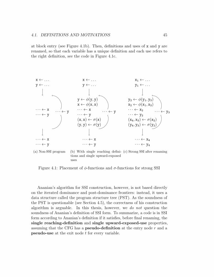
4.1. DEFINITIONS AND MOTIVATIONS 45
at block entry (see Figure 4.1b). Then, definitions and uses of x and y arerenamed, so that each variable has a unique definition and each use refers tothe right definition, see the code in Figure 4.1c.
x← . . .y← . . .
· · · ← x
· · · ← y· · · ← y
· · · ← x
· · · ← y
(a) Non-SSI program
x← . . .y← . . .
y← φ(y, y)x← φ(x, x)· · · ← x
· · · ← y
(x, x)← σ(x)(y, y)← σ(y)
· · · ← y
· · · ← x
· · · ← y
(b) With single reaching defini-tions and single upward-exposeduses
x1 ← . . .y1 ← . . .
y2 ← φ(y1, y3)x2 ← φ(x1, x3)· · · ← x2· · · ← y2(x4, x3)← σ(x2)(y4, y3)← σ(y2)
· · · ← y3
· · · ← x4· · · ← y4
(c) Strong SSI after renaming
Figure 4.1: Placement of φ-functions and σ-functions for strong SSI
Ananian’s algorithm for SSI construction, however, is not based directlyon the iterated dominance and post-dominance frontiers: instead, it uses adata structure called the program structure tree (PST). As the soundness ofthe PST is questionable (see Section 4.5), the correctness of his constructionalgorithm is arguable. In this thesis, however, we do not question thesoundness of Ananian’s definition of SSI form. To summarize, a code is in SSIform according to Ananian’s definition if it satisfies, before final renaming, thesingle reaching-definition and single upward-exposed-use properties,assuming that the CFG has a pseudo-definition at the entry node r and apseudo-use at the exit node t for every variable.
46 CHAPTER 4. SSA EXTENSIONS: SSI
4.1.2 Singer’s definition of SSI
Singer, in his Ph.D. thesis [29], proposed an alternative definition of SSI form:a program is in SSI form if, before renaming (and a fortiori after renam-ing), it satisfies both the dominance property and the post-dominanceproperty. As we explained in chapter 2, the post-dominance property isthe symmetric of the dominance property, inverting the role of uses anddefinitions. It means that, for each variable, any use that is upward-exposedat a definition of the variable post-dominates this definition (such a use isthus unique). After renaming, as there is a single definition per variable, the(unique) definition of each variable is post-dominated by all its uses, and onlyone is upward-exposed at the definition.
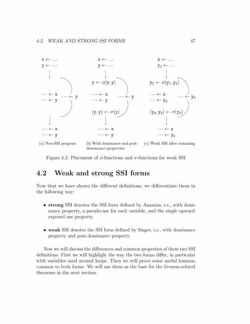
Singer assumed (incorrectly, as we will show) that this definition wasequivalent to Ananian’s. It is true that Ananian’s definition does satisfythe post-dominance property; however, Singer’s definition does not implythe single upward-exposed use property for all program points, only fordefinition points as we explain in Section 4.2.1. Therefore, situations existwhere Ananian’s definition of SSI form leads to the instantiation of moreσ-functions than with Singer’s definition. An example is given in Figure 4.2.Now, with Singer’s definition, the situation is different for x and y. The twouses of x post-dominate its unique definition, so no σ-function is needed and,consequently, no φ-function either. For y, the use on the back-edge doesnot post-dominate the definition of y, thus a σ-function is added at the endof the central block, then a φ-function at the entry of the basic block (seeFigure 4.2b). Then, definitions and uses of y are renamed, leading to thecode of Figure 4.2c.
4.1.3 Semi-pruned and pruned SSI form
Similar in principle to SSA form, semi-pruned, and pruned variants of SSIform can be defined. It is worth saying that the pseudo-use considered byAnanian’s definition is only used to guide the placement of σ-functions duringSSI construction. It does not alter the live-range of a variable, as doing sowould cause all variables defined locally in the procedure to interfere at theexit point, which is not, in fact, the case.
For the sake of simplicity, we assume pruned SSI form, unless statedotherwise.
4.2. WEAK AND STRONG SSI FORMS 47
x← . . .y← . . .
· · · ← x
· · · ← y· · · ← y
· · · ← x
· · · ← y
(a) Non-SSI program
x← . . .y← . . .
y← φ(y, y)
· · · ← x
· · · ← y
(y, y)← σ(y)
· · · ← y
· · · ← x
· · · ← y
(b) With dominance and post-dominance properties
x← . . .y1 ← . . .
y2 ← φ(y1, y3)
· · · ← x
· · · ← y2
(y4, y3)← σ(y2)
· · · ← y3
· · · ← x
· · · ← y4
(c) Weak SSI after renaming
Figure 4.2: Placement of φ-functions and σ-functions for weak SSI
4.2 Weak and strong SSI forms
Now that we have shown the different definitions, we differentiate them inthe following way:
• strong SSI denotes the SSI form defined by Ananian, i.e., with domi-nance property, a pseudo-use for each variable, and the single upward-exposed use property,
• weak SSI denotes the SSI form defined by Singer, i.e., with dominanceproperty and post-dominance property.
Now we will discuss the differences and common properties of these two SSIdefinitions. First we will highlight the way the two forms differ, in particularwith variables used around loops. Then we will prove some useful lemmas,common to both forms. We will use them as the base for the liveness-relatedtheorems in the next section.
48 CHAPTER 4. SSA EXTENSIONS: SSI
4.2.1 Weak and strong SSI forms are not equivalent
Figures 4.1 and 4.2 illustrate the difference between the two definitions of SSIform. Both definitions insert one φ-function and one σ-function for variable y;the difference is observed with respect to variable x. As we just discussed, thedifferent key properties for inserting φ-functions and σ-functions are linkedas follows:
1. the single reaching-definition property, with pseudo-definitions, is equiv-alent to the dominance property;
2. the single upward-exposed-use property, with pseudo-uses, implies thepost-dominance property; this is not an equivalence as illustrated inFigures 4.1 and 4.2.
The subtle difference between the single upward-exposed use property andthe post-dominance property is the following. If the post-dominance propertyholds, then, before renaming, every use of a variable that is upward-exposedat a definition of the variable is required to post-dominate this definition. Asthe post-dominance relation forms a tree, this implies that, for each definition,there is a single upward-exposed use (possibly the pseudo-use, unless prunedSSI is considered). On the contrary, if the single upward-exposed use propertyis satisfied, then for any program point p, not necessarily a definition, thereis a single upward-exposed use u. This implies that p is post-dominated by u,otherwise there is a path from p to u and a path from p to the pseudo-use atthe CFG exit node t, not containing u, and the single upward-exposed useproperty is not satisfied for p.
Thus, a procedure that has been converted to strong SSI form also satisfiesthe criteria for weak SSI form. Strong SSI enforces the single upward-exposeduse property for all program points, pruned SSI for the entire live-range, andweak SSI only for all definitions. As our example illustrates, these conditionsare not equivalent. For SSA, the situation is different as enforcing the singlereaching-definition property for all uses is equivalent to enforcing it for theentire live-range. To summarize, after renaming, for both weak and strongSSI forms, the unique definition of a variable dominates all its uses andeach use post-dominates its definition. In (pruned) strong SSI, an additionalproperty is true: considering that each variable has a pseudo-use at the CFGexit node, then, for each program point of the live-range, there is a uniqueupward-exposed use.
4.2. WEAK AND STRONG SSI FORMS 49
4.2.2 Properties of variables in weak and strong SSIforms
Variables in SSI form satisfy certain properties, common to weak and strongSSI forms, which we will exploit in our proofs regarding the structure oflive-ranges.
Let x be a variable in (strong or weak) SSI form and let d be its (unique)definition point. In (strong or weak) SSI form, each use of x post-dominatesd and the post-dominance relation forms a tree. Therefore, all uses belongto a path, in the post-dominator tree, from t, the CFG exit node, to d inthe post-dominator tree (note that paths in the post-dominator tree take thereverse direction from the CFG, e.g., each CFG node is reachable from t).Therefore, one of these uses post-dominates all other uses. We call this usethe last use of x, and denote it by u.
Let LIVE denote the live-range of x, i.e., the set of program points wherex is live. By definition, for any strict program, p ∈ LIVE if there is a path,in the CFG, from p to some use of x that does not go through d. Becauseall uses of x post-dominate d, and u post-dominates all other uses of x, theprevious path can be extended to form a path from p to u that does notcontain d. In other words, under both strong and weak SSI, LIVE is the setof points p such that there is a path from p to the last use u that does notcontain d.
The next three lemmas hold for any variable x, in either weak or strongSSI. Lemma 5 states that if x is live at a node p of the post-dominance tree,then it is live at all descendants of p that are not descendants of d, i.e., inthe whole subtree rooted at p minus the subtree rooted at d.
Lemma 5. If p ∈ LIVE, p pdom q, and ¬d pdom q, then q ∈ LIVE.
Proof. Since ¬d pdom q, there exists a path, in the CFG, from q to t notcontaining d. Because p pdom q, this path must contain p. Thus, there mustexist a sub-path from q to p that does not contain d. Since p ∈ LIVE, thereexists a path from p to u that does not contain d. By concatenating thesepaths, we can construct a path from q to u that does not contain d; it followsthat q ∈ LIVE.
Lemma 6 states that if x is live at a node p of the post-dominance tree,then it is live at all ancestors of p that are not ancestors of u, i.e., all nodesin the path of the post-dominance tree leading to p and starting from, butexcluding, the least common ancestor of p and u.
50 CHAPTER 4. SSA EXTENSIONS: SSI
Lemma 6. If p ∈ LIV E, q pdom p, and ¬q pdom u, then q ∈ LIVE.
Proof. Since p ∈ LIVE, there is a path, in the CFG, from p to u that doesnot contain d. Because ¬q pdom u, there exists a path from u to t that doesnot contain q. Concatenating the two paths yields a path from p to t via u,such that the sub-path from u to t does not contain q, and the sub-path fromp to u does not contain d. Since q pdom p, this path from p to t must containq, thus q must be in the sub-path from p to u that does not contain d. Thisestablishes the existence of a path from q to u that does not contain d, fromwhich follows q ∈ LIVE.
Lemma 7 states that if x is live at a node p of the post-dominance tree,then the ancestors of d that are not ancestors of p dominate p, i.e., p isdominated by all nodes in the path of the post-dominance tree leading to dand starting from, but excluding, the least common ancestor of p and d.
Lemma 7. If p ∈ LIVE, q pdom d, and ¬q pdom p, then q dom p.
Proof. Consider a path, in the CFG, from r to p. As p ∈ LIVE, d dom p,thus this path contains d. Since ¬q pdom p, there exists a path from p tot without q. Since q pdom d, q must be included in the path from d to p,otherwise we get a path from d to t without q. It follows that q dom p.
4.3 The intersection graph is an interval graph
This section proves that, for a procedure in either strong or weak SSI form,the interference graph (that is, the intersection graph of the live-ranges, seeSection 3.5) is an interval graph. More precisely, we prove that the nodesof a CFG can be totally ordered so that the live-range of each SSI variablecorresponds to an interval in this linearized representation. Under both strongand weak SSI form, the start point of the interval is the definition of thevariable. Under strong SSI form, the end point of the interval is a use of thevariable, while this is not always true in weak SSI.
Our linearization order is based on the post-dominator tree, the dominancerelation, and, for weak SSI, a connected minimal loop nesting forest, asdescribed in Section 2.2.
4.3. THE INTERSECTION GRAPH IS AN INTERVAL GRAPH 51
4.3.1 Strong SSI form
The total order of blocks we provide in Section 4.3.2 for weak SSI form isof course also suitable for strong SSI form. Nevertheless, as the situation issimpler for strong SSI form, we prefer to define in this section a suitable orderof blocks that is more intuitive and easier to build.
First, we compute a dominance-based order, i.e., a partial order ofblocks that respects the dominance relation. In such an order, if a node ustrictly dominates a node v, then u appears before v. Such an order can becomputed by a topological traversal of the dominator tree. It can also beobtained by a preorder or a reverse postorder of any depth-first search(DFS) of the CFG.
Second, a preorder DFS traversal of the post-dominator tree is performedwith one additional constraint on the order in which the child nodes arevisited. Let u and v be two children of a given node in the post-dominatortree, then the following must hold:
1. Constraint on dominance: if u dom v, then the preorder DFStraversal of the post-dominator tree should visit the subtree rooted atv before it visits the subtree rooted at u.
For that, it suffices to visit the children in the reverse order of the dominance-based order computed in the preceding step. The resulting linearization ofthe CFG nodes is called a reverse strong interval order. It starts at theCFG exit node and ends at the CFG entry node. The third and final stepis to reverse the reverse strong interval order, yielding a strong intervalorder.
Note that an order of nodes (i.e., of basic blocks) extends directly to anorder of program points by traversing all program points within a block fromentry to exit.
Consider the CFG of Figure 4.3a, whose corresponding dominator andpost-dominator trees are shown in Figures 4.3b and 4.3c respectively. To finda dominance-based order, we can compute a DFS of the CFG considering thenodes in preorder:
[1, 2, 3, 4, 7, 8, 9, 11, 12, 5, 6, 10]
Next, we perform a preorder DFS traversal of the post-dominator tree, shownin Figure 4.3c. The children are visited with a priority given by the reversedominance-based order, yielding a reverse strong interval ordering. Forexample, nodes 8 and 11 are both children of node 12 in the post-dominator
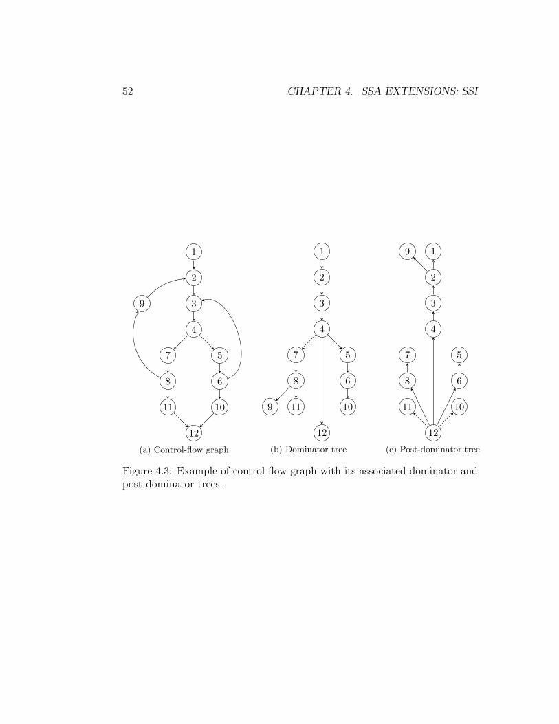
52 CHAPTER 4. SSA EXTENSIONS: SSI
1
2
9 3
4
5
6
10
7
8
11
12
(a) Control-flow graph
1
2
9
3
4
5
6
10
7
8
11
12
(b) Dominator tree
1
2
9
3
4
5
6
10
7
8
11
12
(c) Post-dominator tree
Figure 4.3: Example of control-flow graph with its associated dominator andpost-dominator trees.
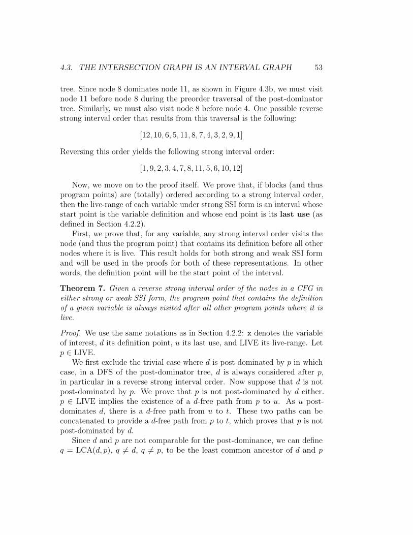
4.3. THE INTERSECTION GRAPH IS AN INTERVAL GRAPH 53
tree. Since node 8 dominates node 11, as shown in Figure 4.3b, we must visitnode 11 before node 8 during the preorder traversal of the post-dominatortree. Similarly, we must also visit node 8 before node 4. One possible reversestrong interval order that results from this traversal is the following:
[12, 10, 6, 5, 11, 8, 7, 4, 3, 2, 9, 1]
Reversing this order yields the following strong interval order:
[1, 9, 2, 3, 4, 7, 8, 11, 5, 6, 10, 12]
Now, we move on to the proof itself. We prove that, if blocks (and thusprogram points) are (totally) ordered according to a strong interval order,then the live-range of each variable under strong SSI form is an interval whosestart point is the variable definition and whose end point is its last use (asdefined in Section 4.2.2).
First, we prove that, for any variable, any strong interval order visits thenode (and thus the program point) that contains its definition before all othernodes where it is live. This result holds for both strong and weak SSI formand will be used in the proofs for both of these representations. In otherwords, the definition point will be the start point of the interval.
Theorem 7. Given a reverse strong interval order of the nodes in a CFG ineither strong or weak SSI form, the program point that contains the definitionof a given variable is always visited after all other program points where it islive.
Proof. We use the same notations as in Section 4.2.2: x denotes the variableof interest, d its definition point, u its last use, and LIVE its live-range. Letp ∈ LIVE.
We first exclude the trivial case where d is post-dominated by p in whichcase, in a DFS of the post-dominator tree, d is always considered after p,in particular in a reverse strong interval order. Now suppose that d is notpost-dominated by p. We prove that p is not post-dominated by d either.p ∈ LIVE implies the existence of a d-free path from p to u. As u post-dominates d, there is a d-free path from u to t. These two paths can beconcatenated to provide a d-free path from p to t, which proves that p is notpost-dominated by d.
Since d and p are not comparable for the post-dominance, we can defineq = LCA(d, p), q 6= d, q 6= p, to be the least common ancestor of d and p
54 CHAPTER 4. SSA EXTENSIONS: SSI
in the post-dominance tree. Let p′ and d′ be the corresponding children ofq. More formally, ipdom(p′) = ipdom(d′) = q, d′ pdom d, and p′ pdom p.Now, ¬p′ pdom d, by construction of p′, and u pdom d, by definition of SSI.It follows that ¬p′ pdom u. Since p′ pdom p, by construction of p′, andp ∈ LIVE, Lemma 6 ensures that p′ ∈ LIVE. Finally, because d′ pdom d, byconstruction of d′, and ¬d′ pdom p′, by construction of d′ and p′, Lemma 7proves that d′ dom p′. It follows that d′ and its descendant d is visited afterp′ and its descendant p in a reverse strong interval order. This is due to thecriterion for choosing children during the preorder DFS of the post-dominatortree: the reverse of the dominance order.
The next theorem characterizes the live-range of a variable in strong SSIas the descendants, in the post-dominator tree, of its last use, minus thedescendants of its definition.
Theorem 8. In strong SSI form, the live-range of a variable is the set ofprogram points post-dominated by its last use but not post-dominated by itsdefinition.
Proof. Again, let x denote the variable of interest, d its definition point, u itslast use, and LIVE its live-range. Recall that d dom u and u pdom d.
First, we show that u pdom p for every point p ∈ LIVE. Assume to thecontrary that there exists a path from p to t that does not go through u.Since p ∈ LIVE, there is also a path from p to u. The existence of thesetwo different paths contradicts the single upward-exposed-use property ofstrong SSI form, for at least one point, for example the point where they split.Therefore, the complete live-range is included in the set of descendants of u inthe post-dominator tree. Conversely, Lemma 5 shows that any descendant ofu that is not a descendant of d belongs to LIVE. Finally, if p is a descendantof d, all paths in the CFG from p to u contain d, thus p cannot belong toLIVE.
This yields our main result, in the case of strong SSI.
Theorem 9. In a strong interval order, the live-range of a variable in strongSSI form corresponds to an interval. Moreover, this interval starts at thedefinition point of the variable and ends at its last use.
Proof. This follows from Theorems 7 and 8. In a reverse strong intervalorder, which is a preorder DFS of the post-dominator tree, the last use of
4.3. THE INTERSECTION GRAPH IS AN INTERVAL GRAPH 55
a variable is encountered before all the points it post-dominates. Then, thesubtrees rooted at its children are completely traversed, one after the other,the last one being the subtree that contains the definition of the variable, asTheorem 7 shows. Furthermore, according to Theorem 8, all points traversedthis way before reaching the variable definition correspond exactly to thelive-range of the variable.
Corollary 1. For a procedure in strong SSI form, the interference graph, i.e.,the intersection graph of the live-ranges, is an interval graph.
Proof. This follows immediately from Theorem 9.
4.3.2 Weak SSI form
For weak SSI form, the general scheme of block linearization requires botha post-dominator tree and a connected minimal loop nesting forest. Theconstruction of the order is similar to the strong interval order: first buildan auxiliary order, then do a preorder DFS traversal of the post-dominatortree using the previous order, and finally reverse it. The difference is that,during the preorder DFS traversal of the post-dominator tree in the secondstep, one additional constraint is imposed on the order in which children of agiven node are processed. Let u, v, and w be children of a given node in thepost-dominator tree. The two constraints that the order must now satisfy areas follows:
1. Constraint on dominance: If u dom v, then the preorder DFStraversal of the post-dominator tree should visit the subtree rooted atv before it visits the subtree rooted at u.
2. Constraint on the loop nesting forest: if u and v belong to thesame loop, and w does not, then the subtree rooted at w should not bevisited between the subtrees rooted at u and v.
A total order resulting from such a traversal is called a reverse weakinterval order and its reversal is called a weak interval order. Next, weprove that such an order satisfying both constraints exists.
Lemma 1 shows that any topological order of FL(G) respects the domi-nance if L is a connected minimal loop forest. In other words, when defininga reverse weak interval order, the two constraints used to decide which sub-tree to traverse next are not contradictory. If the second constraint (the
56 CHAPTER 4. SSA EXTENSIONS: SSI
constraint on the loop nesting forest) is satisfied, the first one (the constrainton dominance) will be automatically satisfied. In particular, we call the ordergiven by [27, Theorem 4] a loop-dominance-based order.
Consider, the example of Figure 4.4. As explained in Section 2.2, the CFGdepicted in Figure 4.4a has two nested loops: L1 = {2, 3, 4, 5, 6, 7, 8, 9} andL2 = {3, 4, 5, 6}. Due to the edges between the different strongly connectedcomponents encountered during the construction of the loop forest and thenesting of loops, this CFG has only two possible loop-dominance-based orders:
[1, 2, 3, 4, 5, 6, 7, 8, 9, 10, 11, 12] (or 10 and 11 inverted)
Now, we perform a preorder DFS traversal of the post-dominator tree (shownin Figure 4.3c) where the children of each node are visited according to thereverse loop-dominance-based order; in particular, node 8 must be visitedbefore node 6. This provides us with the following reverse weak interval order:
[12, 11, 10, 8, 7, 6, 5, 4, 3, 2, 9, 1]
Reversing this order yields the following weak interval order:
[1, 9, 2, 3, 4, 5, 6, 7, 8, 10, 11, 12]
for which, as we will show, the live-range of any variable in weak SSI is aninterval.
Theorem 10. In a weak interval order, the live-range of a variable in weakSSI form corresponds to an interval.
Proof. Again, let x denote the variable of interest, d its definition point, u itslast use, and LIVE its live-range. Let ≤ denote a weak interval order. ByTheorem 7, we already know that d ≤ p for any program point p ∈ LIVE. Toestablish that the live-range corresponds to an interval, it remains to provethat q ∈ LIVE and d < p < q imply p ∈ LIVE, for any two points p and q.
The order ≤ respects the post-dominance, as it is based on a preorderDFS traversal of the post-dominator tree; thus ¬d pdom p and ¬p pdom q.If q pdom d, then q pdom p due to the preorder DFS traversal of the post-dominator tree, and p ∈ LIVE by Lemma 5. Similarly, u pdom p impliesp ∈ LIVE by Lemma 5 (recall that u pdom d, u ∈ LIVE, and ¬d pdom p).Therefore, we can assume that ¬u pdom p and ¬q pdom d.
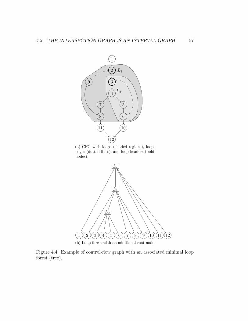
4.3. THE INTERSECTION GRAPH IS AN INTERVAL GRAPH 57
1
2
9 3
4
5
6
10
7
8
11
12
L1
L2
(a) CFG with loops (shaded regions), loop-edges (dotted lines), and loop headers (boldnodes)
1 2 3 4 5 6 7 8 9 10 11 12
Lr
L1
L2
(b) Loop forest with an additional root node
Figure 4.4: Example of control-flow graph with an associated minimal loopforest (tree).
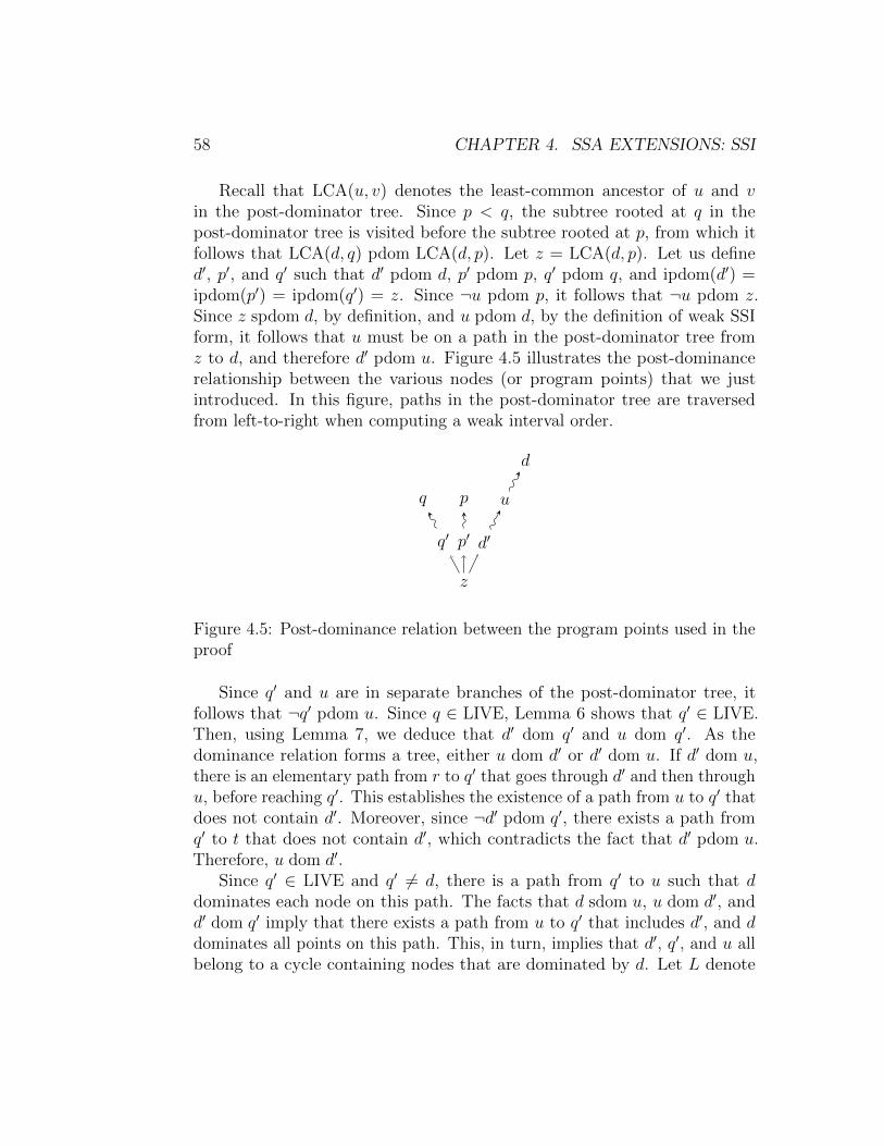
58 CHAPTER 4. SSA EXTENSIONS: SSI
Recall that LCA(u, v) denotes the least-common ancestor of u and vin the post-dominator tree. Since p < q, the subtree rooted at q in thepost-dominator tree is visited before the subtree rooted at p, from which itfollows that LCA(d, q) pdom LCA(d, p). Let z = LCA(d, p). Let us defined′, p′, and q′ such that d′ pdom d, p′ pdom p, q′ pdom q, and ipdom(d′) =ipdom(p′) = ipdom(q′) = z. Since ¬u pdom p, it follows that ¬u pdom z.Since z spdom d, by definition, and u pdom d, by the definition of weak SSIform, it follows that u must be on a path in the post-dominator tree fromz to d, and therefore d′ pdom u. Figure 4.5 illustrates the post-dominancerelationship between the various nodes (or program points) that we justintroduced. In this figure, paths in the post-dominator tree are traversedfrom left-to-right when computing a weak interval order.
d
u
d′
p
p′
q
q′
z
Figure 4.5: Post-dominance relation between the program points used in theproof
Since q′ and u are in separate branches of the post-dominator tree, itfollows that ¬q′ pdom u. Since q ∈ LIVE, Lemma 6 shows that q′ ∈ LIVE.Then, using Lemma 7, we deduce that d′ dom q′ and u dom q′. As thedominance relation forms a tree, either u dom d′ or d′ dom u. If d′ dom u,there is an elementary path from r to q′ that goes through d′ and then throughu, before reaching q′. This establishes the existence of a path from u to q′ thatdoes not contain d′. Moreover, since ¬d′ pdom q′, there exists a path fromq′ to t that does not contain d′, which contradicts the fact that d′ pdom u.Therefore, u dom d′.
Since q′ ∈ LIVE and q′ 6= d, there is a path from q′ to u such that ddominates each node on this path. The facts that d sdom u, u dom d′, andd′ dom q′ imply that there exists a path from u to q′ that includes d′, and ddominates all points on this path. This, in turn, implies that d′, q′, and u allbelong to a cycle containing nodes that are dominated by d. Let L denote
4.3. THE INTERSECTION GRAPH IS AN INTERVAL GRAPH 59
the loop in the loop nesting forest such that the removal of the loop-edges ofL breaks this circuit. At least one node on this circuit must be a loop-headerfor L. Therefore, d /∈ L, since d dominates each node on the circuit, and aloop-header cannot be dominated by any other node within the loop when itis a loop-entry node.
Now, recall that d′, p′, and q′ are all children of z in the post-dominatortree, and that the preorder DFS traversal of the dominator tree, whichconstructs the reverse weak interval ordering, processes the subtrees rootedat the children of z in reverse loop-dominance-based order. Specifically, p′
must occur between q′ and d′ in the reverse loop-dominance-based order. Thefact that the reverse loop-dominance-based order respects the loop nestingproperty implies that p′ ∈ L. Therefore, there exists a path from p′ to u in L,thus it does not contain d, which proves that p′ ∈ LIVE. Finally, Lemma 5shows that p ∈ LIVE too.
Theorem 10, therefore, proves that the live-range of each variable underweak SSI corresponds to an interval in a total order of CFG nodes. Moreover,this order depends only on the structure of the CFG and not on the relativepositions of definitions and uses of variables within the basic blocks of theCFG. This order can thus be pre-computed to help with liveness analysis, asdescribed in the following section, and it remains unchanged even if varioustransformations move or delete instructions, as long as the CFG structure isnot modified. Note however that some forms of code motion may require theinsertion of additional φ-functions and σ-functions in order to preserve weakSSI form.
Corollary 2. For a procedure in weak SSI form, the interference graph, i.e.,the intersection graph of the live-ranges, is an interval graph.
Proof. This follows immediately from Theorem 10.
The primary difference between strong and weak SSI is the “end” of theinterval corresponding to the live-range of each variable. Under strong SSI,the end of the interval is the last use of the variable and it post-dominates allpoints of the live-range. Under weak SSI, the end of the interval may not bea use and it does not necessarily post-dominate all points of the live-range.Figure 4.3 illustrates these points: if a variable is defined in node 1 and usedonly in node 3, weak SSI does not require the insertion of any φ-functionsor σ-functions: the initial live-range is not split and the variable is live
60 CHAPTER 4. SSA EXTENSIONS: SSI
everywhere in the two loops, i.e., its live-range spans all CFG nodes 1 through9. In particular, there is no point in the live-range that post-dominates theentire live-range. The strong interval order proposed in Section 4.3.1 wouldbe incorrect here because 11 is between 1 and 6, but the variable is notlive in 11. With the weak interval order proposed in Section 4.3.2 for weakSSI, the live-range is an interval, its end point is node 8, and 8 does notpost-dominate 6.
4.4 Liveness under SSI
Since we proved our results on the properties of live-range in the previoussection, we can now find out what the consequences are in term of liveness forvariables under SSI. The live-range of variables all have a particular shape,this property leads to a much simpler liveness analysis.
In principle, it should be possible to convert minimal or semi-pruned SSIform to pruned SSI form using dead code elimination. This ensures thatall σ-functions and φ-functions corresponding to a variable x in the pre-SSIprogram are placed at points where x was originally live, and liveness analysisis not required to ensure this property. We may still require liveness analysisin SSI form, either to perform register allocation or to eliminate as manycopies as possible during SSI elimination. One possibility is to computeliveness analysis prior to building SSI form, and then updating the resultsto account for the fact that the conversion to SSI partitions each pre-SSIvariable into a set of smaller variables; the other possibility is to performliveness analysis once the procedure has been converted to SSI form.
This section points out a consequence of Theorem 9: under strong SSIform, iterative data-flow analysis is not required. Instead, it suffices totraverse the nodes of the CFG in reverse strong interval order and, withineach node, to traverse the instructions in reverse order. During this traversal,a variable is live exactly from the first time one of its uses is encountered(which is guaranteed to be the last use) until its definition is processed. Theconsequences of this approach are twofold:
1. If live sets are explicitly required, neither data-flow equations norunion of sets are needed throughout the traversal: the live-out setof a basic block is exactly the live-in set of the previously-processedblock. Dataflow analysis is reduced to its simplest form: a single passover the control-flow graph is enough.
4.5. SINGLE-ENTRY SINGLE-EXIT REGION AND SSI 61
2. Register allocators based on linear scan [26] approximate the lifetimeof each variable as an interval, rather than an exact live-range. AnSSI-based implementation of a linear scan register allocator can computelive intervals exactly without the need to compute live sets explicitly.
This fast approach to liveness analysis does not directly work for weakSSI form since there may be no last use that post-dominates each point wherea variable is live. If the basic algorithm outlined above is applied, a pointwhere a variable becomes live may be encountered using the reverse weakinterval order before the last use is encountered. Instead, we need to identify,for each variable, the last point (in the order) of the largest loop in the loopnesting forest that contains its last use but not its definition. This will bethe end of the interval, as the proof of Theorem 10 shows. Be careful, thisproperty is not due to the fact that the order of blocks respects the nestingof the loops as this is not true in general for a weak or strong interval order.If this last point is pre-computed, the liveness analysis can be performed ina unique pass, as for strong SSI, following the reverse weak interval order.Another solution is to first compute, for each variable, an incomplete intervalfrom its definition to its last use, then to extend it in a second pass, followingthe weak interval order and exploiting the structure of the loop forest.
Once liveness analysis has been performed, the interval property implies asimple O(1)-time query to determine whether a variable x is live at a givenpoint p in a procedure. Under strong SSI form, the endpoints of the intervalare the definition point d and the final use u of x; therefore, x is live at pif and only if d ≤ p ≤ u using a strong interval order. Under weak SSI,one endpoint of the live interval is d, and liveness analysis must be run inadvance to determine the other endpoint, which we denote as q. Therefore,x is live at a point p if and only if d ≤ p ≤ q using a weak interval order.Similarly, computing live-in and live-out sets can be done in one pass, oncethese intervals are identified.
4.5 Single-entry single-exit region and SSI
We will now clarify some of the mistakes made during the creation of SSI andfound in subsequent uses of the SSI form.
When Ananian first presented SSI, his motivation was the simplificationof backward data-flow algorithms. Because he would split the live-rangesat the post-dominance frontier, a backward data-flow analysis, which would
62 CHAPTER 4. SSA EXTENSIONS: SSI
only gather information form uses and definition would become sparse: theinformation can be attached to the variables.
But the subsequent papers, who used SSI as a basis, do not use thisproperty. Most people mistakenly thought that SSI would split at branchpoints and could be used to gather precise information from conditional.
What SSI effectively does is splitting the live range of a variable so thatmore contextual information can be attached to the variable name. Butdepending of the information that is wanted, more or less splits are needed.We can differentiate between several cases:
• information propagates backward and only change where uses are placed
• information propagates forward and can change even if there is no usesof the variable, for example at branch points where a related variable ischecked
In the first case, the necessary split points are at the post-dominancefrontier, that is the strong SSI form. In the second case, more splits can beneeded. If the information that is computed is needed not only at the use anddefinition points, but at every point of the live-range, then a split after everybranch point where information is gained and the variable is live is needed.That is the way e-SSA, a variant of the SSA form presented by Bodik etal. [5], splits the live-ranges to help solve the array bound checking problem.Otherwise if the information is only needed at use-def points, a form withless splits can be used.
Weiss [32] gives a definition of what he considers relevant program points:the set of branch point relevant to the execution of the program point x isthe set of branch points such that there exists a path from the branch pointto the exit node, and another path to x, and both paths are disjoint exceptfor the branch point. Furthermore, as we recalled earlier, Weiss proved thatthe iterated set S+(x, exit), is equal to the non iterated set S(x, exit), andthat this set is equal to the post-dominance frontier of x. This means thatwhenever two nodes share the same set of relevant branch point, the executionof one node implies the execution of the other, and any information gainedfrom a branch point is valid for both points.
This notion of relevance and the implied splitting at the relevant points isin fact the form defined by Ananian’s in his pessimistic algorithm. Similarlyto the dependence flow graph by Johnson et al. [23], his algorithm wouldsplit whenever the use points and the definition point would be in different
4.5. SINGLE-ENTRY SINGLE-EXIT REGION AND SSI 63
single-entry single-exit regions. Single-entry single exit regions are related tothe notion of relevant points: two nodes share the same set of relevant branchpoints iff they are contained in the same set of SESE regions.
4.5.1 Single-entry single-exit region
Ananian’s algorithm for (strong) SSI construction [2] is based on an auxiliarydata structure called the program structure tree (PST) [22]. The PSTdecomposes the control flow graph into a hierarchy of canonical single-entrysingle-exit (SESE) regions. Extending the notion of dominance and post-dominance to edges instead of just nodes, a SESE region is formed by apair of CFG edges (ei, ej) if ei dom ej, ej pdom ei, and ei and ej are loop-cycle equivalent, meaning that every cycle in the CFG that contains ei alsocontains ej, and vice-versa.
A SESE region (ei, ej) is defined to be canonical if ej dom ek for anySESE region (ei, ek) and ei pdom ek for any SESE region (ek, ej). Thehierarchy of canonical SESE regions is based on the following definition ofcontainment: SESE region (ei, ej) contains a basic block b if ei dom b andej pdom b.
This notion of containment does not match the intuitive definition of SESEregions, we assume that a SESE region is a connected region of the control flowgraph, while Johnson et al. definition does not ensure that property. Figure 4.6shows an example where a SESE region is not a connected subgraph.
Moreover using their definition of SESE region, the following was stated atheorem:
If R1 and R2 are two canonical SESE regions of a CFG, theneither R1 and R2 are node-disjoint, or R1 is contained within R2
(or vice-versa).
But as shown in our example, (A,B) and (B,C) are both canonical SESEregions. However, both contain the basic block b, as per the definitionof containment provided above. Therefore, it is impossible to construct ahierarchy of SESE regions, given this definition of containment.
The theorem itself contains three parts, and parts 1 and 3 wrongly assumethat “an edge cannot both dominate and post-dominate a node”. In theexample of Figure 4.6, the three edges A, B, and C both dominate andpost-dominate the node (i.e., basic block) b. Actually, reasoning with nodes(and not edges), it is not possible to construct an order of the nodes of a CFG
64 CHAPTER 4. SSA EXTENSIONS: SSI
that respects both the dominance and post-dominance relations, i.e., an orderdenoted by ≤ such that u ≤ v if u dom v and u ≤ v if v pdom u. Such anorder cannot exist because the header node of a for-loop or a while-loop maysimultaneously dominates and post-dominates every other node in the loop,as shown in Figure 4.7. Thus, it is impossible to construct an order underwhich the header occurs both before and after each node in the loop.
The following definition for SESE would make the theorem on programstructure tree hierarchy correct:
Definition 3. A SESE region is a connected subgraph of G = (V,E), suchthat there exists a unique incoming edge from outside the region, and a uniqueoutgoing edge to outside the region.
This definition directly matches the intuitive concept of single-entry single-exit, furthermore we can show that a SESE region defined this way is also aSESE region as defined by Johnson et al.
Proof. The incoming edge obviously dominates any node from the region(and thus the outgoing edge), similarly the outgoing edge post-dominatesevery node from the region (and the incoming edge). Let us show that ourtwo distinguished (incoming and outgoing) edges are cycle equivalent. Givena cycle containing the incoming edge. Since the source of the incoming edgeis not in the SESE region but its target is, there exists an edge from the cyclesuch that its source is part of the SESE region, but its target is not. But ourdefinition of SESE states that this edges is unique, it is the outgoing edge ofthe SESE. Similarly we can show that every cycle containing the outgoingedge must contain the incoming edge.
Similarly given two edges following Johnson’s definition, we can showthey are the incoming and outgoing edges of a SESE region matching ourdefinition: we only need to show that there is a subgraph of the control flowgraph such that they are incoming and outgoing edges.
Given an SESE region with edges (e1, e2), and the set of nodes such that:
• they are dominated by e1, and not dominated by e2
• they are post-dominated by e2, and not post-dominated by e1
Let us show this set form a connected subgraph.
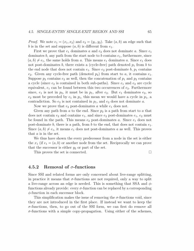
4.5. SINGLE-ENTRY SINGLE-EXIT REGION AND SSI 65
Proof. We note e1 = (x1, x2) and e2 = (y1, y2). Take (a, b) an edge such thatb is in the set and suppose (a, b) is different from e1.
First we prove that e1 dominates a and e2 does not dominate a. Since e1dominates b, any path from the start node to b contains e1, furthermore, since(a, b) 6= e1, the same holds from a. This means e1 dominates a. Since e1 doesnot post-dominates b, there exists a (cycle-free) path denoted p1 from b tothe end node that does not contain e1. Since e2 post-dominate b, p1 containse2. Given any cycle-free path (denoted p2) from start to a, it contains e1.Suppose p2 contains e2 as well, then the concatenation of p1 and p2 containsa cycle (since e2 is contained in both sub-paths). Since e1 and e2 are cycleequivalent, e1 can be found between this two occurrences of e2. Furthermoresince, e1 is not in p2, it must be in p1, after e2. But e1 dominates e2, soe2 most be preceded by e1 in p1, this mean we would have a cycle in p1, acontradiction. So e2 is not contained in p1, and e2 does not dominate a.
Now we prove that e2 post-dominates a while e1 does not.Given any path from a to the end. Since p2 is a path from start to a that
does not contain e2 and contains e1, and since e2 post-dominates e1, e2 mustbe found in the path. This means e2 post-dominates a. Since e1 does notpost-dominate b, there is a path, from b to the end, that does not contain e1.Since (a, b) 6= e1, it means e1 does not post-dominates a as well. This provesthat a is in the set.
We thus have shown the every predecessor from a node in the set is eitherthe x1 (if e1 = (a, b) or another node from the set. Reciprocally we can provethat the successor is either y2 or part of the set.
This proves the set is connected.
4.5.2 Removal of σ-functions
Since SSI and related forms are only concerned about live-range splitting,in practice it means that σ-functions are not required, only a way to splita live-range across an edge is needed. This is something that SSA and φ-functions already provide: every σ-function can be replaced by a correspondingφ-function in each successor block.
This simplification makes the issue of removing the σ-functions void, sincethey are not introduced in the first place. If instead we want to keep theσ-functions, then, to go out of the SSI form, we can first do remove allσ-functions with a simple copy-propagation. Using either of the schemes,
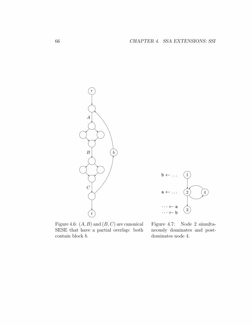
66 CHAPTER 4. SSA EXTENSIONS: SSI
r
t
b
A
B
C
Figure 4.6: (A,B) and (B,C) are canonicalSESE that have a partial overlap: bothcontain block b.
1b← . . .
2a← . . .
3· · · ← a
· · · ← b
4
Figure 4.7: Node 2 simulta-neously dominates and post-dominates node 4.
4.5. SINGLE-ENTRY SINGLE-EXIT REGION AND SSI 67
once we removed the σ-functions, going out of SSI is now the same problemas going out of SSA which we will explore in the next chapter.

68 CHAPTER 4. SSA EXTENSIONS: SSI
Chapter 5
SSA Destruction
5.1 Motivations
A naive SSA destruction increases even more the number of new variablesand the code size, because φ-functions are replaced by variables and copiesfrom or to these variables. A solution, especially useful for JIT compilation,is to introduce copies on the fly, during the SSA destruction, and only whenneeded, as in Method III of Sreedhar et al. [31]. Also, to eliminate copiesor to avoid introducing them, some interference information, and thus someliveness information, is required. Thanks to the dominance property in SSA,one can avoid building explicitly the interference graph. Also, thanks to thenotion of dominance forest, Budimlic et al. [13] proposed a SSA destructionmechanism, more suitable for JIT compilation, as it reduces the number ofinterference tests.
In light of previous work, our primary goal was to design a new SSAdestruction, suitable for JIT compilation, thus focused on speed and memoryfootprint, as previous approaches were not fully satisfactory. However, to makethis possible, we had to revisit the way the SSA destruction is conceptuallymodeled. We then realized that our framework not only can target speed, butalso addresses the problem of correctness and of efficiency (i.e., quality ofthe resulting code).
Several papers have already addressed the SSA destruction problem. Wepropose a new method because, first, we want to rely on a provably-correctmethod, generic, simple to implement, without special cases and patches,and in which correctness and quality of the result (i.e., optimization) are
69
70 CHAPTER 5. SSA DESTRUCTION
conceptually separated. And secondly, we want to develop a technique thatcan be fast and not too memory-consuming, without compromising correctnessand quality. Let us first go back to previous approaches.
SSA destruction was first mentioned in the seminal paper by Cytron etal. [18, Page 478]:
“Naively, a k-input φ-function at entrance of a node X can bereplaced by k ordinary assignments, one at the end of each controlflow predecessor of X. This is always correct, but these ordinarystatements sometimes perform a good deal of useless work. If thenaive replacement is preceded by dead code elimination and thenfollowed by coloring, however, the resulting code is efficient”.
In other words, copies are placed in predecessor blocks to emulate the φ-function semantics and Chaitin-style coalescing [15] (as in register allocation)is used to remove some of them.
Although this naive translation seems, at first sight, correct, it can leadto subtle errors as pointed by Briggs et al. [9, Page 880] because of parallelcopies and/or critical edges in the control flow graph. Two typical situationsare identified, the “lost copy problem” and the “swap problem”, some patchesare proposed to handle them correctly, and a “more complicated algorithmthat includes liveness analysis and a preorder walk over the dominator tree” isquickly presented for the general cases, but with neither a discussion of com-plexity, nor a correctness proof. Nevertheless, according to the authors, thissolution “cures the problems that [they] have seen in practice” [9, Page 879].
The first solution, both simple and correct, was proposed by Sreedhar etal. [31]. In addition to the copies at the end of each control flow predecessor,the trick is to insert another copy at the entry of the basic block of the φ-function. This simple mechanism, detailed hereafter, is sufficient to make thetranslation always correct, except for special cases that we point out. Severalstrategies are then proposed to introduce as few copies as possible, includinga special rule to eliminate more copies than with standard coalescing and sothat “copies that it places cannot be eliminated by the standard interferencegraph based coalescing algorithm” [31, Page 196]. This last (also unproved)claim turns out to be correct, but only for the very particular way copiesare inserted, i.e., always after the previously-inserted copies in the sameblock. Also, the way coalescing is handled is again more a patch, driven byimplementation considerations, than a conceptual choice. We will come back
5.2. CLEAN APPROACH 71
to this point later. Nevertheless, our technique is largely inspired by thevarious algorithms of Sreedhar et al.
In other words, these previous approaches face some conceptual subtletiesthat make them sometimes incorrect, incomplete, overly pessimistic, or tooexpensive. This is mostly due to the fact that a clean definition of interferencefor variables involved in a φ-function is lacking, while it is needed both forcorrectness (for adding necessary copies) and for optimization (for coalescinguseless copies). Our first contribution, beyond algorithmic improvements,is to address this key point. Thanks to this interference definition, wedevelop a conceptually SSA destruction framework, in which correctnessand optimization are not intermixed. The resulting implementation is muchsimpler, with no special cases, and we can even develop fast algorithms foreach independent phase, without compromising the quality of results. Therest of this section gives an overview of our technique, before diving into moredetailed explanations.
5.2 Clean approach
Consider a φ-function a0 ← φ(a1, . . . , an) placed at entry of a block B0: a0takes the value of ai if the control-flow comes from the i-th predecessorblock of B0. If a0, . . . , an can be given the same name without changingthe semantics of the program, the φ-function can be eliminated. When thisproperty is true, the SSA form is said to be conventional (CSSA) [31]. Thisis not always the case: after copy propagation or code motion, some ofthe ai may “interfere” with each other (this SSA form is sometimes calledtransformed SSA form, TSSA). The technique of Sreedhar et al. [31] consistsin three steps:
1. translate SSA into CSSA, thanks to the introduction of copies;
2. eliminate redundant copies;
3. eliminate φ-functions and leave CSSA.
In their first method (Method I), the translation into CSSA is done asfollows. For each φ-function a0 ← φ(a1, . . . , an) at entry of block B0:
• n+ 1 new variables a′0, . . . , a′n are introduced;
72 CHAPTER 5. SSA DESTRUCTION
• a copy a′i ← ai is placed at the end of Bi, the i-th predecessor block ofB0;
• a copy a0 ← a′0 is placed at entry of the block B0 (after φ-functions);
• the φ-function a0 ← φ(a1, . . . , an) is replaced by a′0 ← φ(a′1, . . . , a′n).
If a block contains several φ-functions, then several copies needs to beintroduced. They are introduced at the same place and they should be viewedas parallel copies. This is what we do here, as Leung and George in [25].However, as far as correctness is concerned, they can be sequentialized in anyorder, as they concern different variables. This is what Sreedhar et al. do inall their methods.
Lemma 8. After the introduction of the new variables a′i for all φ-functionsand the corresponding copies, the code is in CSSA form. In other words,replacing all variables a′i by a new unique variable for each φ and removingall φ-functions is a correct SSA destruction.
Proof. First note that, after introduction of the copies, the code semanticsis preserved. The variables ai are copied into the variables a′i, then fed intothe new φ-function to create a′0, which is finally copied into a0. To show thatthe code is in CSSA, note that the variables a′i have very short live ranges.The variables a′i, for i > 0, are defined at the very end of disjoint blocks Bi,thus none is live at the definition of another: they do not interfere. The sameis true for a′0 whose live range is located at the very beginning of B0, evenif B0 may be equal to Bi for some i. Thus, the n+ 1 variables a′i can sharethe same variable name, as they are never simultaneously live on a givenexecution path.
It is now clear why the proposal of Cytron et al. was wrong. Without thecopy from a′0 to a0, the φ-function defines directly a0. The live range of a0can be long enough to intersect with on of the a′i, i > 0: it is the case if a0 islive-out of the block Bi where a′i is defined. Two cases are possible: eithera0 is used in a successor of Bi 6= B0, in which case the edge from Bi to B0 iscritical (as in the “lost copy problem”), or a0 is used in B0 as a φ-functionargument (as in the “swap problem”). In the latter case, if parallel copiesare used, a0 is dead before a′i is defined but, if copies are without taking careof potential conflicts, the live range of a0 can go beyond the definition pointof a′i and lead to incorrect code after renaming a0 and a′i with the same name.
5.2. CLEAN APPROACH 73
As Lemma 8 explains, splitting the definition of the φ-function itself withone additional variable at the block entry solves the problem. In the methodsof Sreedhar et al., the decision to keep the copy a′i (in Method I) or to insertit (in Method III) depends on the intersection of the live range of a′i with thelive-out set of the block Bi. But this techniques hides a subtlety: what does“at the end of basic block” mean? Depending on the branching instruction,the copies cannot always be inserted at the very end of the block, i.e., after allvariables uses and definitions. For example, for a φ-function after a conditionalbranch that uses a variable u, the copies must be inserted before the use of u.Since any new copy that is inserted might interfere with u, the intersectioncheck have to be done with u as well, otherwise some incorrect code can begenerated. Consider the SSA code in Figure 5.1(a), which is not under CSSAform. As u is not live-out of block B2, the optimized algorithm (Method III)of Sreedhar et al. considers that, in order to transform the code into CSSAform, it is sufficient to insert a copy v′ of v at the end of B2. But the copy isinserted before the use of u (Figure 5.1(b)) and the code is still not CSSA sinceu and v′ interfere. Removing the φ-function, i.e., giving the same name to w,u, and v′ leads to the incorrect code of Figure 5.1(c). This problem, nevermentioned in the literature, needs to be solved for implementors. Fortunately,it is easy to correct by considering the intersection with the set of variableslive just after the point of copy insertion, in our case the live-out set with theaddition of u, instead of simply the live-out set of the block.
An even more subtle case can happen, when the basic block containsvariables defined after the point of copy insertion. This configuration is possiblein embedded environments, where some DSP-like branching instructions havea behavior similar to a hardware loop: in addition to the condition, a counteru is decremented by the instruction itself. If u is used in a φ-function ina direct successor block, no copy insertion can split its live range. In thiscase, it must then be given the same name as the variable defined by theφ-function. If both variables interfere, we cannot use the same name for bothvariables. In order to solve the problem, SSA could be used with more careinside the compiler: either we avoid promoting the variable to SSA, someinstruction can be changed, or the control-flow edge can be split. While itmight not happen in general purpose computer, this point has never beenmentioned before: SSA destruction by copy insertion alone is not alwayspossible, in presence of complex branching instructions. For example, supposethat for the code of Figure 5.2(a), the instruction selection chooses a branchwith decrement (denoted Br dec) for Block B1 (Figure 5.2(c)). Then, the
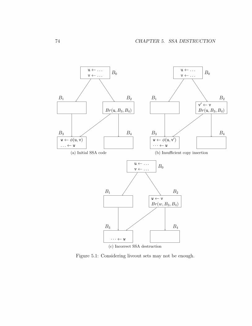
74 CHAPTER 5. SSA DESTRUCTION
u← . . .v← . . .
B0
B1
Br(u, B3, B4)
B2
w← φ(u, v). . .← w
B3 B4
(a) Initial SSA code
u← . . .v← . . .
B0
B1
v′ ← v
Br(u, B3, B4)
B2
w← φ(u, v′)· · · ← w
B3 B4
(b) Insufficient copy insertion
u← . . .v← . . .
B0
B1
w← v
Br(w,B3, B4)
B2
· · · ← w
B3 B4
(c) Incorrect SSA destruction
Figure 5.1: Considering liveout sets may not be enough.
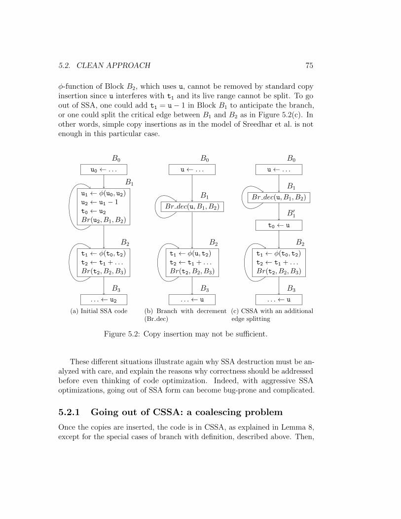
5.2. CLEAN APPROACH 75
φ-function of Block B2, which uses u, cannot be removed by standard copyinsertion since u interferes with t1 and its live range cannot be split. To goout of SSA, one could add t1 = u− 1 in Block B1 to anticipate the branch,or one could split the critical edge between B1 and B2 as in Figure 5.2(c). Inother words, simple copy insertions as in the model of Sreedhar et al. is notenough in this particular case.
u0 ← . . .
B0
u1 ← φ(u0, u2)u2 ← u1 − 1t0 ← u2Br(u2, B1, B2)
B1
t1 ← φ(t0, t2)t2 ← t1 + . . .Br(t2, B2, B3)
B2
. . .← u2
B3
(a) Initial SSA code
u← . . .
B0
Br dec(u, B1, B2)
B1
t1 ← φ(u, t2)t2 ← t1 + . . .Br(t2, B2, B3)
B2
. . .← u
B3
(b) Branch with decrement(Br dec)
u← . . .
B0
Br dec(u, B1, B2)
B1
t0 ← u
B′1
t1 ← φ(t0, t2)t2 ← t1 + . . .Br(t2, B2, B3)
B2
. . .← u
B3
(c) CSSA with an additionaledge splitting
Figure 5.2: Copy insertion may not be sufficient.
These different situations illustrate again why SSA destruction must be an-alyzed with care, and explain the reasons why correctness should be addressedbefore even thinking of code optimization. Indeed, with aggressive SSAoptimizations, going out of SSA form can become bug-prone and complicated.
5.2.1 Going out of CSSA: a coalescing problem
Once the copies are inserted, the code is in CSSA, as explained in Lemma 8,except for the special cases of branch with definition, described above. Then,
76 CHAPTER 5. SSA DESTRUCTION
going out of CSSA is straightforward: all variables involved in a φ-function canbe given the same name and the φ-functions can be removed. This solves thecorrectness aspect. To improve the code however, it is important to remove asmany useless copies as possible. This can be treated as a classical coalescingproblem, as in register allocation. The difference resides in the complexity:with Method I, the number of new copies and variables can be very large,which can be too costly, especially if a interference graph is used. Sreedhar etal. propose several improvements. The first proposed improvement consists ofthe introduction of copies only when variables interfere and the conservativeupdate of the interference graph (Method II). A second technique consists ofa more involved algorithm that also uses and updates liveness information(Method III). Finally a special “SSA based coalescing” can be used, that isuseful to complement Method I and Method II but is useless after Method III.Those improved techniques all rely on the explicit representation of congruenceclasses partitioning the program variables into the sets of variables that arealready coalesced together.
Sreedhar et al. use special coalescing rules depending on the method, butthis approach can be simplified. Actually, once the code is in CSSA, theoptimization problem is a standard aggressive coalescing problem (i.e., withno constraints on the number of target variables) and we should be able touse standard heuristics for this NP-complete problem [28, 8]. The fact thatthe code is in SSA does not make it simpler or special. Also, Method IIIturns out to give better results than Method I followed by coalescing, eventhough Method III was primarily designed for speed. This result can beexplained with the fact that Sreedhar et al. rely on a conservative definitionof interferences in order to decide if two variables can be given be same name(coalesced). As we have discussed in Section 3.5, we can easily exploit theSSA properties to identify when two variables have the same value: in thiscase, they do not interfere even if their live ranges intersect. Then, with thisintrinsic definition of interferences, there is no point to compare, in terms ofquality of results, a method that introduces all copies first as in Method Ior on the fly as in Method III: they are equivalent. Furthermore, since ourdefinition of interferences is more accurate, more copies can be removed.
Another weakness in the model of Sreedhar et al. is the lack of flexibilityin the placement of copies, they are inserted in a sequential order at the endor entry of a block. We prefer to stick to the SSA semantics, i.e., to rely onparallel copies (all sources of every copy are read before any write occurs).We then sequentialize these copies afterward, once we know which copies
5.2. CLEAN APPROACH 77
remain. The interest is two-fold. First, with sequential copies, some additionalinterferences between the corresponding variables appear. This gives lessfreedom to the coalescer, especially if we take into account additional registerconstraints. Second, with parallel copies, we avoid a tricky update of livenessinformation. Our approach allows us to handle all copies in a uniform way,this is fundamental to minimize the engineering effort.
In conclusion, with a more accurate definition of interferences, the useof parallel copies, and a generic coalescing algorithm to eliminate copies,we achieve our goal: a conceptually simple approach, provably correct, inwhich correctness and optimization are separated. This is of important forimplementing SSA in an industrial compiler in order to avoid complex bugs.We can now give an overview of the general process before detailing eachindividual step.
5.2.2 Overview of the SSA destruction
To summarize, conceptually, our SSA destruction process has five successivephases:
1. Insert parallel copies for all φ-functions using in Method I of Sreedharet al. and coalesce all a′i together.
2. Build the interference graph with an accurate definition of interference,using the “SSA value” of variables..
3. Perform aggressive coalescing, possibly with renaming constraints.
4. Go out of CSSA by giving the same name to all coalesced variables.
5. Sequentialize parallel copies, possibly with one more variable and someadditional copies, when swaps are needed.
Step 4 is straightforward. We already explained Step 1 in Section 5.2.Step 2 was detailed in previous chapter, in Section 3.5). Our accurate notionof interference allows us to avoid rebuilding or updating the interferencegraph, furthermore there is no need to rebuild or update the interferencegraph, no need to develop a special SSA-based coalescing algorithm as in [31],and no need to make a distinction between variables which can be coalescedwith Chaitin’s approach or not. The only important information is the factthat they interfere or not.
78 CHAPTER 5. SSA DESTRUCTION
We will now describe Step 3 (Section 5.2.3), and Step 5 (Section 5.2.4).Since correctness (Step 1) and optimization (Step 3) are independent, we
can develop algorithms to make the whole process fast enough for just-in-timecompilation. This will be explained in Section 5.3: fast live-range intersectiontest (Section 5.3.1), fast interference test and node merging (Section 5.3.2),“virtualization” of initial copy insertion (Section 5.3.3), i.e., copy insertion onthe fly similar to Method III of Sreedhar et al. These techniques allow us toskip the construction of the liveness information and the interference graph,and help us lowering the memory footprint.
5.2.3 Coalescing
As previously explained, the SSA destruction is nothing but a traditionalaggressive coalescing problem with no constraints on the number of colors.If all copies are initially inserted, as in Method I of Sreedhar et al., anysophisticated technique can be used. In particular, it is possible to useweights to first examine copies placed in inner loops: this approach reducesthe number of static and dynamically-executed copies. Contrary to Sreedharet al. which do not use weights, we use a classical profile information to getbasic blocks frequency. However this weight may be slightly under-estimated:if a swap is needed in order to sequentialize a parallel copy, additional copywill be required (see Section 5.2.4).
We call virtualization the process of inserting copies on the fly, similarlyto the Method III of Sreedhar et al. With this technique, the copy variablesa′i are created only when needed, but all the reasoning is done as if they wereinserted. To make this possible, we need to consider φ-functions in a certainorder, this will have an impact on the coalescing. Also, Sreedhar et al. use adeferred copy insertion mechanism that, even if not expressed in these terms,amounts to build some maximal independent set of variables (i.e., the setof variables that do not interfere), which are then coalesced. This approachgives indeed slightly better results than reasoning one copy at a time. Inour virtualized version, we also process one φ-function at a time, and simplyconsider its related copies by decreasing weight.
We also address the problem of “copy sharing”. Consider again theexample of two successive copies b = a and c = a. Thanks to our definition ofvalue, the fact that b is live at the definition of c does not necessarily implythat b and c interfere. Suppose however that a interferes with b and c for someother reason. In this case, no coalescing would occur although coalescing b and
5.2. CLEAN APPROACH 79
c would save one copy, by “sharing” the copy of a. Leung et al. [25] provideexamples ABI constraints where this situation occurs. This sharing problemis difficult to model and optimize, in fact deciding the insertion point of thecopies is even harder, but we can still provide some optimizations. We cancoalesce two variables b and c if they are both copies of the same variable aand if their live ranges intersect. We restrict ourself to intersecting live-rangesbecause if they are disjoint, the optimization could increase the live range ofthe dominating variable, thus possibly creating some interference not takeninto account. Section 5.2.5 mentions this important post-optimization, whichis a benefit provided by our value-based interference definition.
5.2.4 Sequentialization of parallel copies
In every steps of the algorithm, we treat the copies placed by Step 1 at theend or entry of a given block as parallel copies. This indeed matches closelythe semantics of φ-functions. As we explained previously, this gives us severalbenefits: a simpler implementation, in particular for defining and updatingliveness information, a more symmetrical code, and fewer constraints for thecoalescer. However, since generic parallel copies are not part of any instructionset, at the end of the process, we need to go back to standard code, i.e., writethe final copies in a sequential order. In most cases, we simply need to orderthe copies in the right order, but sometimes an new variable, additional copiesare required. We describe this sequentialization algorithm here.
Conceptually, the algorithm is very simple but deriving a fast implemen-tation is more complicated. Consider the directed graph G whose verticesare the variables involved in the parallel copy and with an edge from a to bwhenever there is a copy from a to b (we write a 7→ b). This graph has thefollowing key property: each vertex has a unique incoming edge, the copy thatdefines it (a parallel copy (b 7→ a, c 7→ a) is possible but only if V (b) = V (c)in which case one of the copies can be removed). Thus, G has a particularstructure: each connected component is a circuit (possibly reduced to onevertex) and each vertex of the circuit can be the root of a directed tree. Agraph with this property is called a windmill graph in the literature. Thecopies of the tree edges can be sequentialized starting from the leaves, copyinga variable to its successors before overwriting it with its final value. Oncethese tree copies are scheduled, it remains to consider the circuit copies. If atleast one vertex of the circuit was the root of a tree, it has already been copiedsomewhere, otherwise, we copy one of the circuit vertices into a new variable.
80 CHAPTER 5. SSA DESTRUCTION
Then, the copies of the circuit can be sequentialized, starting with the copyinto this “saved” vertex and back along the circuit edges. The last copy isdone by moving the saved value in the right variable. Thus, we generatethe same number of copies as expressed by the parallel copy, except possiblyone additional copy for each circuit with no tree edge, i.e., no duplicationof variable. For example, for the parallel copy (a 7→ b, b 7→ c, c 7→ a, c 7→ d),there is one circuit (a, b, c) and an edge from c to d, so we generate the copiesd = c, c = a, a = b, and b = d (and not b = c).
The algorithm emulates a traversal of G (without building it), allowingto overwrite a variable as soon as it is saved in some other variable. Whena variable a is copied in a variable b, the algorithm remembers b as the lastlocation where the initial value of a is available. This information is storedinto resource(a). The initial value that must be copied into b is stored inpred(b). The initialization consists in identifying the variables whose valuesare not needed (tree leaves), which are stored in the list available. Thelist to do contains the destination of all copies to be treated. Copies arefirst treated by considering leaves (while loop on the list available). Then,the to do list is considered, ignoring copies that have already been treated,possibly breaking a circuit with no duplication, thanks to an extra copy intothe fresh variable n.
5.2.5 Qualitative experiments
The experiments were done on the integer subset of the SpecC2000 benchmarkscompiled at aggressive optimization level. The compiler used was an Open64-based production compiler whose code generator exploits the SSA form atmachine level. Renaming register constraints, such as calling conventionsor dedicated registers, are also treated with preliminary copy insertions andcoalesced as copies due to φ-functions.
First, we evaluated how the accuracy of the interference impacts thequality of coalescing. We implemented seven variants of coalescing. Belowa 7→ b is a copy to be removed and X and Y are the congruence classes (seeSection 5.2.1) of a and b that will be merged, in case of coalescing, into alarger class.
Intersect X and Y can be coalesced if there is no variables x ∈ X and y ∈ Ywhose live ranges intersect.
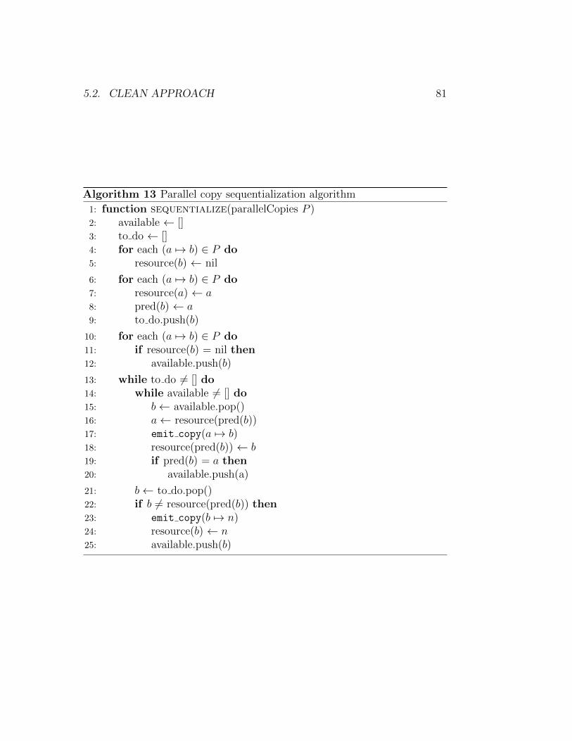
5.2. CLEAN APPROACH 81
Algorithm 13 Parallel copy sequentialization algorithm
1: function sequentialize(parallelCopies P )2: available ← []3: to do ← []4: for each (a 7→ b) ∈ P do5: resource(b) ← nil
6: for each (a 7→ b) ∈ P do7: resource(a) ← a8: pred(b) ← a9: to do.push(b)
10: for each (a 7→ b) ∈ P do11: if resource(b) = nil then12: available.push(b)
13: while to do 6= [] do14: while available 6= [] do15: b← available.pop()16: a← resource(pred(b))17: emit copy(a 7→ b)18: resource(pred(b)) ← b19: if pred(b) = a then20: available.push(a)
21: b← to do.pop()22: if b 6= resource(pred(b)) then23: emit copy(b 7→ n)24: resource(b) ← n25: available.push(b)
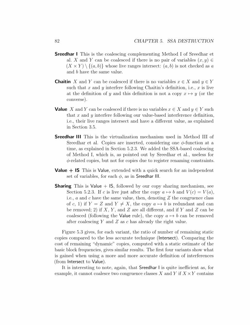
82 CHAPTER 5. SSA DESTRUCTION
Sreedhar I This is the coalescing complementing Method I of Sreedhar etal. X and Y can be coalesced if there is no pair of variables (x, y) ∈(X × Y ) \ {(a, b)} whose live ranges intersect: (a, b) is not checked as aand b have the same value.
Chaitin X and Y can be coalesced if there is no variables x ∈ X and y ∈ Ysuch that x and y interfere following Chaitin’s definition, i.e., x is liveat the definition of y and this definition is not a copy x 7→ y (or theconverse).
Value X and Y can be coalesced if there is no variables x ∈ X and y ∈ Y suchthat x and y interfere following our value-based interference definition,i.e., their live ranges intersect and have a different value, as explainedin Section 3.5.
Sreedhar III This is the virtualization mechanism used in Method III ofSreedhar et al. Copies are inserted, considering one φ-function at atime, as explained in Section 5.2.3. We added the SSA-based coalescingof Method I, which is, as pointed out by Sreedhar et al., useless forφ-related copies, but not for copies due to register renaming constraints.
Value + IS This is Value, extended with a quick search for an independentset of variables, for each φ, as in Sreedhar III.
Sharing This is Value + IS, followed by our copy sharing mechanism, seeSection 5.2.3. If c is live just after the copy a 7→ b and V (c) = V (a),i.e., a and c have the same value, then, denoting Z the congruence classof c, 1) if Y = Z and Y 6= X, the copy a 7→ b is redundant and canbe removed; 2) if X, Y , and Z are all different, and if Y and Z can becoalesced (following the Value rule), the copy a 7→ b can be removedafter coalescing Y and Z as c has already the right value.
Figure 5.3 gives, for each variant, the ratio of number of remaining staticcopies compared to the less accurate technique (Intersect). Comparing thecost of remaining “dynamic” copies, computed with a static estimate of thebasic block frequencies, gives similar results. The first four variants show whatis gained when using a more and more accurate definition of interferences(from Intersect to Value).
It is interesting to note, again, that Sreedhar I is quite inefficient as, forexample, it cannot coalesce two congruence classes X and Y if X×Y contains
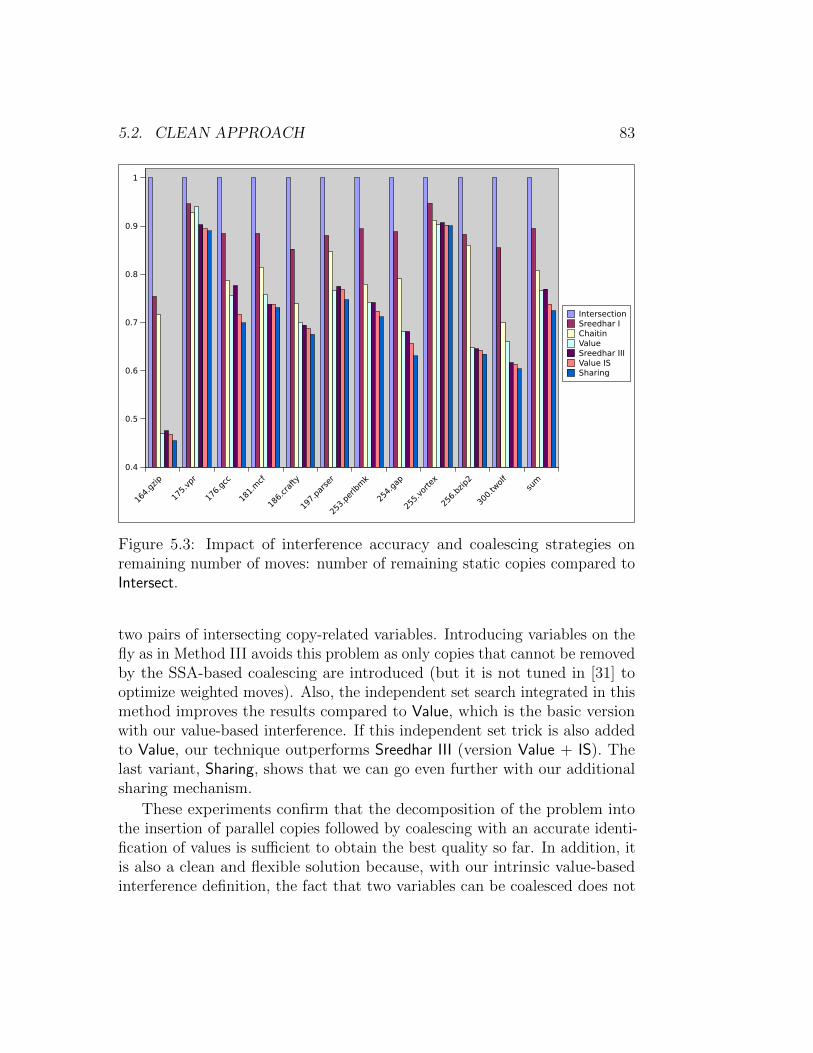
5.2. CLEAN APPROACH 83
164.
gzip
175.
vpr
176.
gcc
181.
mcf
186.
craf
ty
197.
pars
er
253.
perlb
mk
254.
gap
255.
vorte
x
256.
bzip
2
300.
twolf
sum
0.4
0.5
0.6
0.7
0.8
0.9
1
IntersectionSreedhar IChaitinValueSreedhar IIIValue ISSharing
Figure 5.3: Impact of interference accuracy and coalescing strategies onremaining number of moves: number of remaining static copies compared toIntersect.
two pairs of intersecting copy-related variables. Introducing variables on thefly as in Method III avoids this problem as only copies that cannot be removedby the SSA-based coalescing are introduced (but it is not tuned in [31] tooptimize weighted moves). Also, the independent set search integrated in thismethod improves the results compared to Value, which is the basic versionwith our value-based interference. If this independent set trick is also addedto Value, our technique outperforms Sreedhar III (version Value + IS). Thelast variant, Sharing, shows that we can go even further with our additionalsharing mechanism.
These experiments confirm that the decomposition of the problem intothe insertion of parallel copies followed by coalescing with an accurate identi-fication of values is sufficient to obtain the best quality so far. In addition, itis also a clean and flexible solution because, with our intrinsic value-basedinterference definition, the fact that two variables can be coalesced does not
84 CHAPTER 5. SSA DESTRUCTION
depend on the way we introduce copies, either all before coalescing as inMethod I or on the fly as in Method III. With less programming effort, wecan do slightly better than Sreedhar III in terms of quality of results. Moreimportantly, since our framework separates the correctness and the qualityof results from how coalescing is implemented, we can now concentrate onspeed and memory optimizations. These two points are addressed in the nextsection.
5.3 Towards a more efficient algorithm
Implementing the technique of Section 5.2.2 may be too costly. First, itinserts many instructions later considering them as useless, furthermore theinsertion of the copy instructions is expensive as it needs to change theintermediate representation of the code. This process introduces many newvariables as well, and the size of the variable universe has an impact on theliveness analysis and the interference graph, slowing down our algorithm.Also, if a general coalescing algorithm is used, a graph representation withadjacency lists (in addition to the bit matrix) and a working graph to explicitlymerge nodes when coalescing variables, would be required. Additionally theseconstructions, updates, manipulations are not only time-consuming but alsomemory-consuming. We can speed-up the whole process by:
• avoiding the use of a working graph and even of an interference graph,while still relying classical liveness information;
• replacing classical liveness computation by fast liveness checking;
• emulating (“virtualizing”) the introduction of all initial copies, as inMethod III of Sreedhar et al.
If an interference graph is available, it is not clear that using an additionalworking graph is more expensive, but, in the context of aggressive coalescing,both Chaitin [14] and Sreedhar et al. [31] preferred not to use one. To getrid of it, Sreedhar et al. manipulate congruence classes: sets of variablesthat are already coalesced together. Then, two variables can be coalescedif their corresponding congruence classes do not contain any two interferingvariables, one in each congruence class. This quadratic number of variable-to-variable interference tests might be expensive. In Section 5.3.2, we address
5.3. TOWARDS A MORE EFFICIENT ALGORITHM 85
this problem and propose a linear algorithm for interference detection betweentwo congruence classes.
When an interference graph is not available, it is not possible to directlygather the list of variables that interfere with a given variable. Insteadqueries are typically restricted to interference checking, i.e., existence of aninterference. The classical approach consists in computing a full interferencerelation, but stored only as a bit matrix. This needs a costly pre-computationphase: we need to explore the whole program and use live sets to buildinterferences. After this pre-computation, queries are done in constant time.A second approach performs value tests, dominance checks, and livenesschecks, without relying on any pre-computation of live sets. Queries areslightly more time-consuming, but they avoid the use and storage of anyinterference graph. Section 5.3.1 explains the use of such methods.
Finally, Section 5.3.3 explains how we adapt the virtualization mechanismused in Method III of Sreedhar et al., which inserts copies only when needed,to avoid the introduction of many new variables and of useless copies thatwill be removed.
5.3.1 Live-range intersection tests
Remember Section 3.5. We need two tests: a test of live range intersectionand a test of equality of values. In the next section, we explain how wecan check, with this notion of interference, whether two congruence classes(sets of variables already coalesced) interfere. Before, we need an algorithmto decide if two live ranges intersect. Several methods can be used fortesting live-range intersection, either a classical approach building live-in andlive-out sets, or a more refined approach using SSA properties, which we havedescribed in chapter 3.
In the next section, we do not care about the algorithm used in practice,they are used as a black box for developing a linear algorithm that checksinterference between congruence classes.
5.3.2 Linear interference test between two congruenceclasses, with extension to equalities
We now develop one of our main contribution: how to efficiently perform aninterference test between two sets of already-coalesced variables (congruence
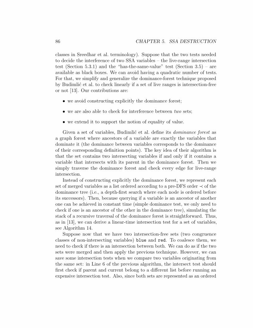
86 CHAPTER 5. SSA DESTRUCTION
classes in Sreedhar et al. terminology). Suppose that the two tests neededto decide the interference of two SSA variables – the live-range intersectiontest (Section 5.3.1) and the “has-the-same-value” test (Section 3.5) – areavailable as black boxes. We can avoid having a quadratic number of tests.For that, we simplify and generalize the dominance-forest technique proposedby Budimlic et al. to check linearly if a set of live ranges is intersection-freeor not [13]. Our contributions are:
• we avoid constructing explicitly the dominance forest;
• we are also able to check for interference between two sets;
• we extend it to support the notion of equality of value.
Given a set of variables, Budimlic et al. define its dominance forest asa graph forest where ancestors of a variable are exactly the variables thatdominate it (the dominance between variables corresponds to the dominanceof their corresponding definition points). The key idea of their algorithm isthat the set contains two intersecting variables if and only if it contains avariable that intersects with its parent in the dominance forest. Then wesimply traverse the dominance forest and check every edge for live-rangeintersection.
Instead of constructing explicitly the dominance forest, we represent eachset of merged variables as a list ordered according to a pre-DFS order ≺ of thedominance tree (i.e., a depth-first search where each node is ordered beforeits successors). Then, because querying if a variable is an ancestor of anotherone can be achieved in constant time (simple dominance test, we only need tocheck if one is an ancestor of the other in the dominance tree), simulating thestack of a recursive traversal of the dominance forest is straightforward. Thus,as in [13], we can derive a linear-time intersection test for a set of variables,see Algorithm 14.
Suppose now that we have two intersection-free sets (two congruenceclasses of non-intersecting variables) blue and red. To coalesce them, weneed to check if there is an intersection between both. We can do as if the twosets were merged and then apply the previous technique. However, we cansave some intersection tests when we compare two variables originating fromthe same set: in Line 6 of the previous algorithm, the intersect test shouldfirst check if parent and current belong to a different list before running anexpensive intersection test. Also, since both sets are represented as an ordered
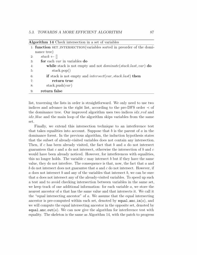
5.3. TOWARDS A MORE EFFICIENT ALGORITHM 87
Algorithm 14 Check intersection in a set of variables
1: function set intersection(variables sorted in preorder of the domi-nance tree)
2: stack ← []3: for each var in variables do4: while stack is not empty and not dominate(stack.last, var) do5: stack.pop()
6: if stack is not empty and intersect(var, stack.last) then7: return true8: stack.push(var)
9: return false
list, traversing the lists in order is straightforward. We only need to use twoindices and advance in the right list, according to the pre-DFS order ≺ ofthe dominance tree. Our improved algorithm uses two indices idx red andidx blue and the main loop of the algorithm skips variables from the sameset.
Finally, we extend this intersection technique to an interference testthat takes equalities into account. Suppose that b is the parent of a in thedominance forest. In the previous algorithm, the induction hypothesis statesthat the subset of already-visited variables does not contain any intersection.Then, if c has been already visited, the fact that b and a do not intersectguarantees that c and a do not intersect, otherwise the intersection of b and cwould have been already noticed. However, for interferences with equalities,this no longer holds. The variable c may intersect b but if they have the samevalue, they do not interfere. The consequence is that, now, the fact that a andb do not intersect does not guarantee that a and c do not intersect. However, ifa does not intersect b and any of the variables that intersect b, we can be surethat a does not intersect any of the already-visited variables. To speed up sucha test and to avoid checking intersection between variables in the same set,we keep track of one additional information: for each variable a, we store thenearest ancestor of a that has the same value and that intersects it. We call itthe “equal intersecting ancestor” of a. We assume that the equal intersectingancestor is pre-computed within each set, denoted by equal anc in(a), andwe will compute the equal intersecting ancestor in the opposite set, denoted byequal anc out(a). We can now give the algorithm for interference test withequality. The skeleton is the same as Algorithm 14, with the patch to progress
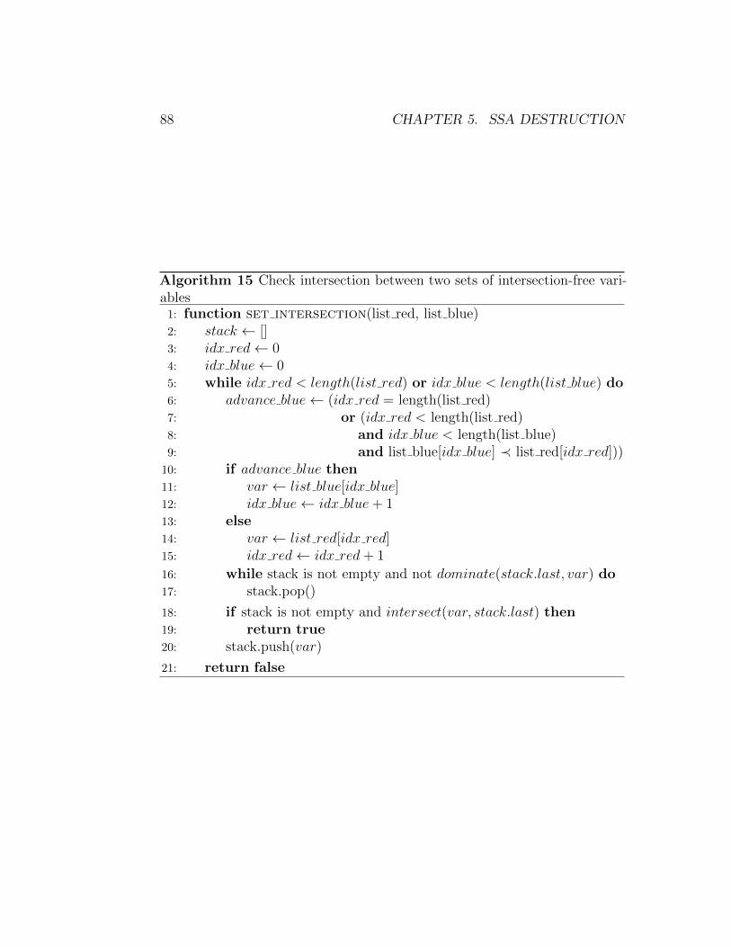
88 CHAPTER 5. SSA DESTRUCTION
Algorithm 15 Check intersection between two sets of intersection-free vari-ables
1: function set intersection(list red, list blue)2: stack ← []3: idx red← 04: idx blue← 05: while idx red < length(list red) or idx blue < length(list blue) do6: advance blue← (idx red = length(list red)7: or (idx red < length(list red)8: and idx blue < length(list blue)9: and list blue[idx blue] ≺ list red[idx red]))
10: if advance blue then11: var ← list blue[idx blue]12: idx blue← idx blue+ 113: else14: var ← list red[idx red]15: idx red← idx red+ 1
16: while stack is not empty and not dominate(stack.last, var) do17: stack.pop()
18: if stack is not empty and intersect(var, stack.last) then19: return true20: stack.push(var)
21: return false
5.3. TOWARDS A MORE EFFICIENT ALGORITHM 89
along the two lists Red and Blue, and where the call Line 14 is now a callto the interference test of Function interference. The principles of thealgorithm are given in the codes themselves. The use of two equal intersectingancestors, in and out, is to make sure that the Function intersect(a, b),which runs a possibly expensive intersection test, is performed only if a and bdo not belong to the same set.
1: function update equal anc out(variable a, variable b)2: tmp← b3: while (tmp 6= NULL) and (intersect(a, tmp) = false do4: tmp ← equal anc in(tmp)
5: equal anc out[a] ← tmp
6: function chain intersect(variable a, variable b)7: tmp ← b8: while (tmp 6= NULL) and (intersect(a, tmp) = false do9: tmp ← equal anc in(tmp)
10: if tmp = NULL then11: return false12: else13: return true14: function interference(variable a, variable b)15: equal anc out(a) = NULL16: if b 6= NULL and (a and b are in the same set) then17: b← equal anc out(b)
18: if b← NULL then19: return false20: if value(a) 6= value(b) then21: return chain intersect(a, b)22: else23: update equal anc out(a, b)
24: return false
We point out that once a list is empty and the stack does not contain anyelement of this list, there is no more intersection or updates to make. Thus,the algorithm can be stopped, i.e., the while loop condition in Algorithm 14can be replaced by:
while (ir < red.size() and nb > 0) or (ib < blue.size() and nr > 0) or (ir <
90 CHAPTER 5. SSA DESTRUCTION
red.size() and ib < blue.size()) do. . .
where nr (resp. nb) are variables that must be implemented to count thenumber of elements of the stack that come from the list Red (resp. Blue).
Finally, if a coalescing of the two sets occurs, it remains to store the twolists as a unique ordered list (in linear time, in a similar joint traversal) andto update the equal intersecting ancestor equal anc in(a) for the combinedset as the maximum (following the pre-DFS order ≺) of equal anc in(a) andequal anc out(a).
5.3.3 Virtualization of φ-nodes
If we implement the whole procedure as described in Section 5.2.2, we startby introducing many new variables a′i (one for each argument of a φ-function,plus its result) and many copies in the block where the φ occurs and in itspredecessors. These variables can be immediately coalesced together, in whatwe call a φ-node, and stored in a congruence class. But, in the data structuresused (interference graph, liveness information, variable name universe, parallelcopy instructions, congruence classes), they exist as data items and consumememory and time, even if at the end, after coalescing, they may disappear.
To avoid the introduction of these initial variables and copies, the techniqueis to emulate the whole process, as does Method III of Sreedhar et al.,which introduces necessary copies on the fly, when they appear to be needed.However, in their method, Sreedhar et al. still manipulate an interference graph(between original variables) and, at each step, update liveness information.Before any related copy is inserted, each argument of a φ-function is consideredto be live-out of the predecessor block it comes from. This is too pessimistic.Also, it is troublesome to maintain the liveness information once copies areinserted: recall the incorrect case of a variable used on a branching operationmentioned in Section 5.2.
Instead, we prefer to use a special location in the code, identified as a“virtual” parallel copy, where the real copies, if any, will be placed. Theoriginal arguments of a φ-function are then assumed, initially, to have a “use”in the parallel copy but are not considered as live-out along the correspondingcontrol flow edge. Then, the algorithm selects copies to coalesce, followingsome order, either a real copy or a virtual copy. If it turns out that a virtualcopy ai 7→ a′i (resp. a′0 7→ a0) cannot be coalesced, the copy is materialized in
5.3. TOWARDS A MORE EFFICIENT ALGORITHM 91
the parallel copy and a′i (resp. a′0) becomes explicit in its congruence class.This way, only copies that the first approach would finally leave uncoalescedare introduced. The only key point to make the emulation of copy insertionpossible is that one should never have to test an interference with a variablethat is not yet materialized or coalesced. For that, φ-nodes are treated one byone, and all virtual copies that imply a variable of the φ-node are considered(either coalesced or materialized) before examining any other copies. Theweakness of this approach is that a global coalescing algorithm cannot be usedbecause only a partial view of the interference graph structure is availableduring the algorithm. However, the algorithm can still be guided by the weightof copies, i.e., the dynamic count associated to the block where it would beplaced if not coalesced. The rest is only a matter of accurate implementation,in particular, it is very important to be careful on how the live ranges ofvariables are updated, following the φ-function semantics.
5.3.4 Results in terms of speed and memory footprint
To measure the potential of our different contributions, in terms of speed-upand memory footprint reduction, we implemented a generic SSA destructionpass that enables us to evaluate different combinations. We selected thefollowing:
Us I Simple coalescing without virtualization. Different techniques for check-ing interferences and liveness are available.
Sreedhar III Native implementation of Method III of Sreedhar et al. com-plemented by their SSA-based coalescing for non φ-related copies. Bothuse an interference graph with a bit-matrix and liveness informationwith ordered sets.
Us III Our implementation of φ-nodes coalescing with virtualization followedby coalescing for non φ-related copies. This implementation is genericenough to support various options: with parallel or sequential copies,with or without an interference graph, with or without live sets. Hence,its implementation is less tuned than Sreedhar III.
By default, Us III and Us I use an interference graph and classical livenessinformation. The options are:
92 CHAPTER 5. SSA DESTRUCTION
InterCheck No interference graph: intersections are checked using a domi-nance test and liveness information as in [13].
InterCheck+LiveCheck No interference graph and no live-in/live-out sets:intersections are checked with the fast liveness checking algorithm of [6].This algorithm, an earlier and more complex variant of the algorithmfrom 3 trades a faster construction time of the needed data structuresfor a slower query time.
Linear+InterCheck+LiveCheck In addition, the linear intersection checkis used instead of the quadratic algorithm.
When an interference graph, liveness sets, or live-check sets are used,timings include their construction. Figure 5.4 shows the timings for thosedifferent variants versus Sreedhar III as a baseline. As one could expect,InterCheck always slows down the execution, while LiveCheck and Linear
always fasten the execution with a significant ratio. A very interesting resultis that the simple SSA-based coalescing algorithm without any virtualizationis as fast as the complex algorithm with virtualization. Indeed, when usingLinear+InterCheck+LiveCheck, adding first all copies and correspondingvariables before coalescing them, do not have the negative impact measuredby Sreedhar et al. any longer.
Figure 5.5 shows the memory footprint used for interference and livenessinformation.
Interference graph is stored using a half-size bit-matrix. Measured pro-vides the measured footprint from the statistics provided by our memoryallocator. In Sreedhar III or Us III, variables are added incremen-tally so the bit-matrix grows dynamically. This leads to a memoryfootprint slightly higher than for a perfect memory. The behaviour ofsuch a perfect memory is evaluated in Evaluated using the formula
d#variables8
e ×#variables/2.
Liveness sets are stored as ordered sets. Measured provides the measuredfootprint of the livesets, without counting those used in liveness con-struction. As for the interference graph, livesets are modified bySreedhar III or Us III. But since the number of simultaneous livevariables do not change, their size remain roughly the same. Becausethe use of ordered sets instead of bit-sets is arguable, we evaluated for
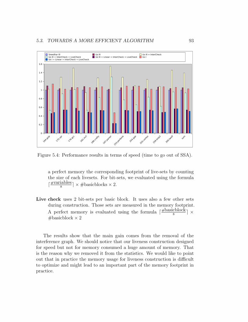
5.3. TOWARDS A MORE EFFICIENT ALGORITHM 93
164.
gzip
175.
vpr
176.
gcc
181.
mcf
186.
craf
ty
197.
pars
er
253.
perlb
mk
254.
gap
255.
vorte
x
256.
bzip
2
300.
twolf
sum
0
0.2
0.4
0.6
0.8
1
1.2
1.4
1.6
Sreedhar III Us III Us III + InterCheckUs III + InterCheck + LiveCheck Us III + Linear + InterCheck + LiveCheck Us IUs I + Linear + InterCheck + LiveCheck
Figure 5.4: Performance results in terms of speed (time to go out of SSA).
a perfect memory the corresponding footprint of live-sets by countingthe size of each livesets. For bit-sets, we evaluated using the formula
d#variables8
e ×#basicblocks× 2.
Live check uses 2 bit-sets per basic block. It uses also a few other setsduring construction. Those sets are measured in the memory footprint.
A perfect memory is evaluated using the formula d#basicblock8
e ×#basicblock× 2
The results show that the main gain comes from the removal of theinterference graph. We should notice that our liveness construction designedfor speed but not for memory consumed a huge amount of memory. Thatis the reason why we removed it from the statistics. We would like to pointout that in practice the memory usage for liveness construction is difficultto optimize and might lead to an important part of the memory footprint inpractice.
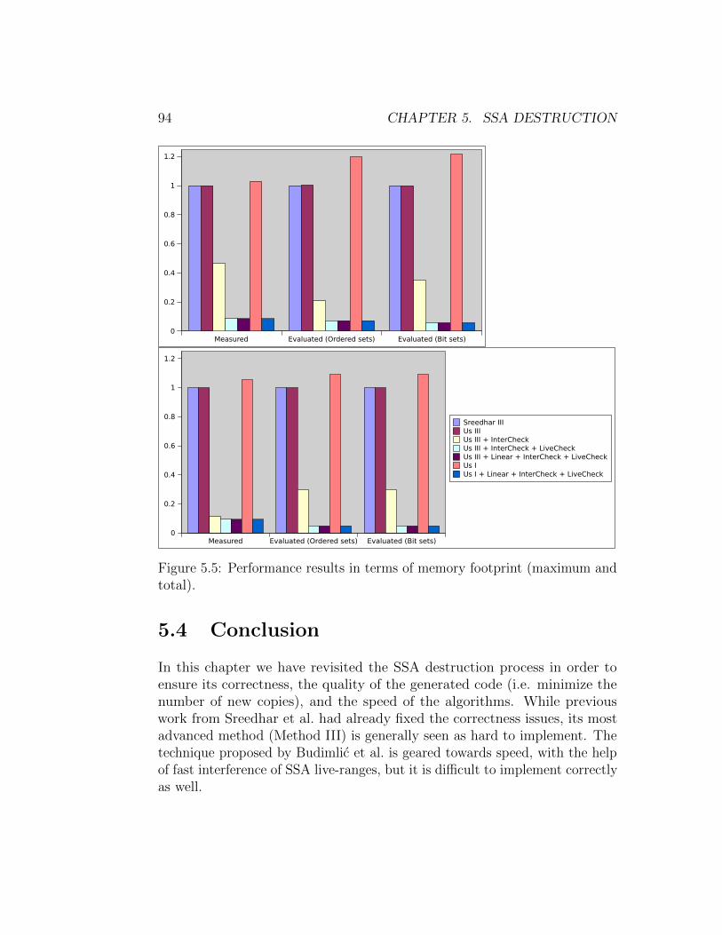
94 CHAPTER 5. SSA DESTRUCTION
Measured Evaluated (Ordered sets) Evaluated (Bit sets)0
0.2
0.4
0.6
0.8
1
1.2
Measured Evaluated (Ordered sets) Evaluated (Bit sets)0
0.2
0.4
0.6
0.8
1
1.2
Sreedhar IIIUs IIIUs III + InterCheckUs III + InterCheck + LiveCheckUs III + Linear + InterCheck + LiveCheckUs IUs I + Linear + InterCheck + LiveCheck
Figure 5.5: Performance results in terms of memory footprint (maximum andtotal).
5.4 Conclusion
In this chapter we have revisited the SSA destruction process in order toensure its correctness, the quality of the generated code (i.e. minimize thenumber of new copies), and the speed of the algorithms. While previouswork from Sreedhar et al. had already fixed the correctness issues, its mostadvanced method (Method III) is generally seen as hard to implement. Thetechnique proposed by Budimlic et al. is geared towards speed, with the helpof fast interference of SSA live-ranges, but it is difficult to implement correctlyas well.
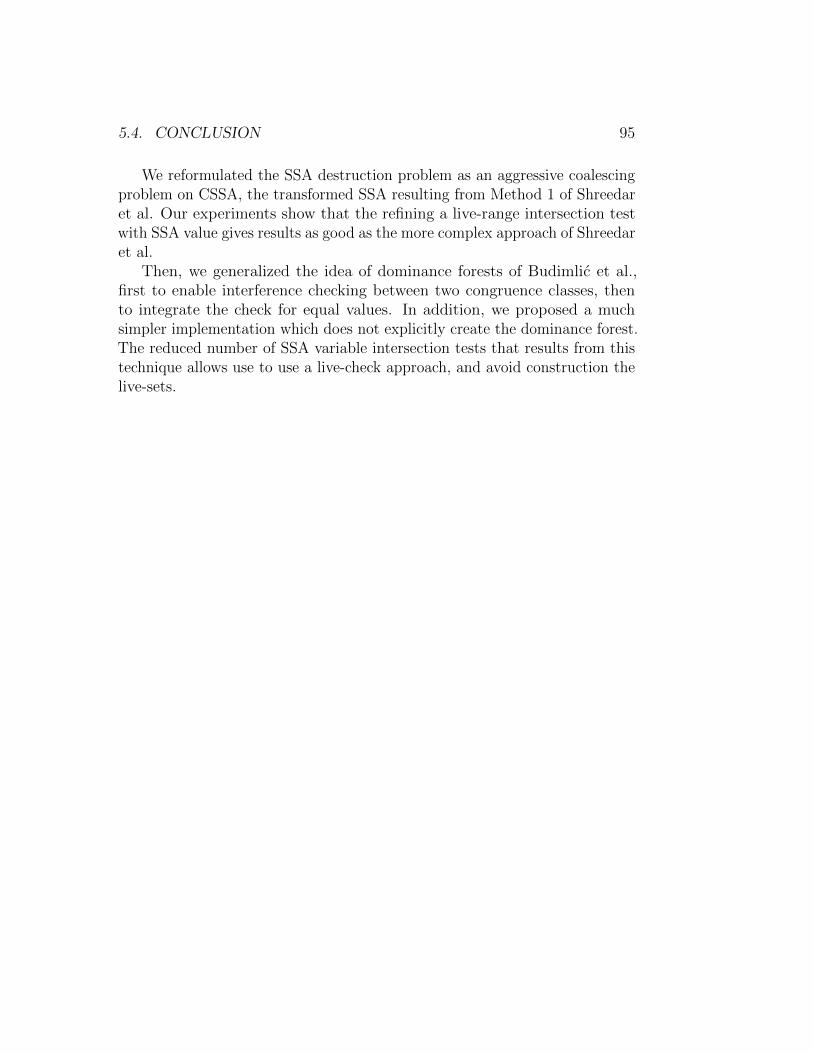
5.4. CONCLUSION 95
We reformulated the SSA destruction problem as an aggressive coalescingproblem on CSSA, the transformed SSA resulting from Method 1 of Shreedaret al. Our experiments show that the refining a live-range intersection testwith SSA value gives results as good as the more complex approach of Shreedaret al.
Then, we generalized the idea of dominance forests of Budimlic et al.,first to enable interference checking between two congruence classes, thento integrate the check for equal values. In addition, we proposed a muchsimpler implementation which does not explicitly create the dominance forest.The reduced number of SSA variable intersection tests that results from thistechnique allows use to use a live-check approach, and avoid construction thelive-sets.

96 CHAPTER 5. SSA DESTRUCTION
Chapter 6
Conclusion
In this thesis we presented three main contributions around liveness, staticsingle information, and SSA destruction.
6.1 Liveness
First, in chapter 3, we presented a novel way to build the live-sets associatedwith a basic block for variables under SSA form. Our technique based onthe loop property bounds the number of time each basic block is visited,there is only two passes compared to the more classic data-flow algorithmwhich usually requires as many iteration as the depth of the loop forest ofthe control flow graph.
More interestingly we presented a different way to look at the livenessproblem, instead of asking the question ”what are the live variables as thestart of the basic block?” (live-set) we instead ask ”is the variable live at thisprogram point?” (live-check). As we have shown, there exists an algorithmto answer this question which requires a much lighter pre-computed datastructures than the live-set problem. But while the pre-computation is muchfaster and requires less memory, the drawback is that each query is morecomplex than a simple lookup in a set, the loop nesting forest needs to beinspected and reachability is tested for each use. This means that the runtimegain will depend on the number of queries. In practice, this threshold isusually favorable, for example the SSA destruction (see chapter 5), can reduceits runtime cost by using the liveness-query approach.
From an engineering point of view, the algorithm is interesting, as the
97
98 CHAPTER 6. CONCLUSION
pre-computed data structures only depend on the shape of the control flowgraph. This means that even if the code is modified, as long as it does notchange the shape of the CFG, no pre-computation is needed. This is anadvantage compared to the classical live-set approach, where a change of thecode can trigger some tedious update of the live-sets.
Our final contribution for this chapter is a simple and precise way to lookat interference. As shown by Chaitin et al., the problem of interference isnot only a problem of intersection of live-ranges. The value of the variablesthemselves matters as well. Fortunately, the use of the SSA form, with itsunique definition for every variable vastly simplifies the analysis of equalitiesof variables. This approach is also used in our SSA destruction algorithmfrom chapter 5.
6.2 Static Single Information form
Then in chapter 4, we explored an SSA variant, the static single informationform. As the various definitions were inconsistent, we clarified them andexplained their differences. We show that the original SSI form from Ananian(strong SSI) differ from the definition given by Singer (weak SSI form), asthey do not split the live-range in the same way when the live-range of avariable at a loop exit point.
Even if the two form differ, we show that for both of them, the intersectiongraph of the live-ranges of the variables under SSI form is an interval graph.But our result is in fact even stronger, as our proof is constructive, we givean order of the control flow graph, depending only on the CFG, not on thevariables themselves, such that every live-range form a consecutive interval.
Finally we explored the implication for liveness analysis of the result. Forexample, this means that the liveness can be stored in a very sparse way:only the start and end of the interval are required.
6.3 SSA destruction
Finally in chapter 5, we revisited the SSA destruction. Our approach simplifiesthe previous techniques, we first transform the code into CSSA form, addingcopies as needed. In a second time, a classical aggressive coalescing is used toremove the useless copies. The simplicity of the approach allows us to easily
6.4. PERSPECTIVES 99
prove the correctness of the algorithm, which was not the case of the previouswork in the area.
We then extend the work from chapter 3, using the notion of interferencewith values to reach remove as many useless copies as possible during thecoalescing phase. This leads us to a generated code quality as good as previousmore complex approaches.
Still using the work from chapter 3, in particular the liveness checkingapproach, we design fast algorithms for the whole approach. In particular,we present an fast algorithm to check interference between sets of variables,using the dominance property from SSA form to avoid useless tests, andusing the single definition property to check for equality of values (refinedinterference test). This approach avoids building the liveness sets, whichmakes our algorithm faster.
6.4 Perspectives
We already have some work in progress, the first is related to SSI form. Themotivation behind the SSI form was a simplification of some optimizations andanalyses: the live-range splitting tries to ensure that some class of propertiesis valid all along every different live-range. This means that the informationcan be attached to the variable instead of using a more complex scheme, aswould be the case if it differed in different parts of the live-range.
But the splitting done by SSI is only useful for a very small class ofinformation, what is needed is a complete taxonomy of various analyses andoptimizations. For every algorithm, we should try to determine if we canclassify the information and then find out if a particular live-range splittingis suitable. We hope this work will be useful and will clarify and help peopledecide which variant of SSA they want to use.
Our other project is a fast register allocator based on SSA form. Wecan use the properties of SSA, processing the variables while following thedominance tree (in order to always encounter the definitions before everyuse), and coloring every variable as we encounter them. In order to make thealgorithm fast and suitable for just-in-time compilers, we pick a global colorfor every variable, and re-color locally (inside a basic block) as needed.
Since we make a better use of the SSA properties (live-ranges are sub-tree of the dominance tree), we believe we can achieve better results than

100 CHAPTER 6. CONCLUSION
a more classic linear scan approach, where interval have holes in them.Furthermore, our approach should prove very simple and lead to a straight-forward implementation.
Bibliography
[1] B. Alpern, M. N. Wegman, and F. K. Zadeck. Detecting equality of vari-ables in programs. In Proceedings of the 15th ACM SIGPLAN-SIGACTSymposium on Principles of Programming Languages (POPL’88), pages1–11. ACM, 1988.
[2] C. Scott Ananian. The Static Single Information Form. Technical ReportMIT-LCS-TR-801, Laboratory for Computer Science, MassachusettsInstitute of Technology, September 1999.
[3] Andrew W. Appel and Jens Palsberg. Modern Compiler Implementationin Java. Cambridge University Press, second edition, 2002.
[4] M. Bender and M. Farach-Colton. The LCA problem revisited. LATIN2000: Theoretical Informatics, pages 88–94.
[5] Rastislav Bodık, Rajiv Gupta, and Vivek Sarkar. ABCD: eliminatingarray bounds checks on demand. In PLDI ’00: Proceedings of theACM SIGPLAN 2000 conference on Programming language design andimplementation, pages 321–333, New York, NY, USA, 2000. ACM.
[6] Benoit Boissinot, Sebastian Hack, Daniel Grund, Benoıt Dupontde Dinechin, and Fabrice Rastello. Fast liveness checking for SSA-formprograms. In IEEE/ACM International Symposium on Code Generationand Optimization (CGO’08), pages 35–44. ACM, 2008.
[7] Florent Bouchez, Alain Darte, Christophe Guillon, and Fabrice Rastello.Register allocation and spill complexity under SSA. Technical ReportRR2005-33, LIP, ENS-Lyon, France, August 2005.
[8] Florent Bouchez, Alain Darte, and Fabrice Rastello. On the complexityof register coalescing. In International Symposium on Code Generation
101
102 BIBLIOGRAPHY
and Optimization (CGO’07), pages 102–114. IEEE Computer SocietyPress, March 2007.
[9] P. Briggs, K. D. Cooper, T. J. Harvey, and L. T. Simpson. Practicalimprovements to the construction and destruction of static single as-signment form. Software – Practice and Experience, 28(8):859–881, July1998.
[10] Preston Briggs, Keith D. Cooper, and L. Taylor Simpson. Value num-bering. Software – Practice and Experience, 27(6):701–724, 1997.
[11] Preston Briggs, Keith D. Cooper, and Linda Torczon. Improvements tograph coloring register allocation. ACM Transactions on ProgrammingLanguages and Systems, 16(3):428–455, 1994.
[12] B.Rosen, M.Wegman, and K.Zadeck. Global value numbers and redun-dant computations. In POPL, pages 12 – 27, 1988.
[13] Zoran Budimlic, Keith D. Cooper, Timothy J. Harvey, Ken Kennedy,Timothy S. Oberg, and Steven W. Reeves. Fast copy coalescing andlive-range identification. In ACM SIGPLAN International Conference onProgramming Language Design and Implementation (PLDI’02), pages25–32. ACM Press, June 2002.
[14] G. J. Chaitin. Register allocation & spilling via graph coloring. InProceedings of the 1982 SIGPLAN symposium on Compiler construction,pages 98–101, 1982.
[15] Gregory J. Chaitin, Marc A. Auslander, Ashok K. Chandra, John Cocke,Martin E. Hopkins, and Peter W. Markstein. Register allocation viacoloring. Computer Languages, 6:47–57, January 1981.
[16] K. D. Cooper and L. Torczon. Engineering a Compiler. Morgan Kauf-mann, 2004.
[17] Keith D. Cooper, Timothy J. Harvey, and Ken Kennedy. Iterative Data-Flow Analysis, Revisited. Technical Report TR04-100, Rice University,2002.
[18] Ron Cytron, Jeanne Ferrante, Barry K. Rosen, Mark N. Wegman, andF. Kenneth Zadeck. Efficiently computing static single assignment form
BIBLIOGRAPHY 103
and the control dependence graph. ACM Transactions on ProgrammingLanguages and Systems, 13(4):451 – 490, 1991.
[19] Benoıt Dupont de Dinechin, cois de Ferriere Fran Christophe Guillon,and Arthur Stoutchinin. Code generator optimizations for the ST120DSP-MCU core. In International Conference on Compilers, Architecture,and Synthesis for Embedded Systems (CASES’00), pages 93 – 103, 2000.
[20] Lal George and Andrew W. Appel. Iterated register coalescing. ACMTransactions on Programming Languages and Systems, 18(3), May 1996.
[21] Paul Havlak. Nesting of Reducible and Irreducible Loops. ACM Trans-actions on Programming Languages and Systems, 19(4):557–567, 1997.
[22] Richard Johnson, David Pearson, and Keshav Pingali. The programstructure tree: Computing control regions in linear time. ACM SIGPLANNotices, 29(6):171–185, 1994.
[23] Richard Johnson and Keshav Pingali. Dependence-based program analy-sis. In PLDI ’93: Proceedings of the ACM SIGPLAN 1993 conferenceon Programming language design and implementation, pages 78–89, NewYork, NY, USA, 1993. ACM.
[24] J.B. Kam and J.D. Ullman. Global data flow analysis and iterativealgorithms. Journal of the ACM (JACM), 23(1):158–171, 1976.
[25] Allen Leung and Lal George. Static single assignment form for machinecode. In SIGPLAN Conference on Programming Language Design andImplementation, pages 204–214, 1999.
[26] Massimiliano Poletto and Vivek Sarkar. Linear scan register allocation.ACM Transactions on Programming Languages and Systems, 21(5):895–913, 1999.
[27] G. Ramalingam. On loops, dominators, and dominance frontiers. ACMTransactions on Programming Languages and Systems, 24(5):455–490,2002.
[28] Fabrice Rastello, Francois de Ferriere, and Christophe Guillon. Optimiz-ing translation out of SSA using renaming constraints. In InternationalSymposium on Code Generation and Optimization (CGO’04), pages265–278. IEEE Computer Society Press, 2004.
104 BIBLIOGRAPHY
[29] Jeremy Singer. Static Program Analysis Based on Virtual Register Re-naming. Technical Report UCAM-CL-TR-660, University of Cambridge,Computer Laboratory, February 2006.
[30] Michael D. Smith, Norman Ramsey, and Glenn Holloway. A generalizedalgorithm for graph-coloring register allocation. In ACM SIGPLANInternational Conference on Programming Language Design and Imple-mentation (PLDI’04), pages 277–288. ACM, 2004.
[31] Vugranam C. Sreedhar, Roy Dz-Ching Ju, David M. Gillies, and VatsaSanthanam. Translating out of static single assignment form. In StaticAnalysis Symposium (SAS’99), pages 194 – 204, Italy, 1999.
[32] Michael Weiss. The transitive closure of control dependence: the iteratedjoin. ACM Lett. Program. Lang. Syst., 1(2):178–190, 1992.
[33] M. Wolfe. J+= J. ACM Sigplan Notices, 29(7):53, 1994.


![computations - arXiv · 2008-05-23 · arXiv:cs/0701192v5 [cs.PL] 22 May 2008 The pitfalls of verifying floating-point computations David Monniaux CNRS / Ecole normale sup´erieure´](https://img.pdfslide.us/doc/110x75/5ea43625a6ebd57c6e7efe63/computations-arxiv-2008-05-23-arxivcs0701192v5-cspl-22-may-2008-the-pitfalls.jpg)