Course notes on

Computational Optimal Transport

Gabriel PeyreCNRS & DMA

Ecole Normale Superieuregabriel.peyre@ens.fr

https://mathematical-tours.github.io

www.numerical-tours.com

October 13, 2019

Abstract

These note cours are intended to complement the book [37] with more details on the theory of OptimalTransport. Many parts are extracted from this book, with some additions and re-writing.

Contents

1 Optimal Matching between Point Clouds 21.1 Monge Problem between Discrete points . . . . . . . . . . . . . . . . . . . . . . . . . . . . . . 21.2 Matching Algorithms . . . . . . . . . . . . . . . . . . . . . . . . . . . . . . . . . . . . . . . . . 3

2 Monge Problem between Measures 32.1 Measures . . . . . . . . . . . . . . . . . . . . . . . . . . . . . . . . . . . . . . . . . . . . . . . 32.2 Push Forward . . . . . . . . . . . . . . . . . . . . . . . . . . . . . . . . . . . . . . . . . . . . . 52.3 Monge’s Formulation . . . . . . . . . . . . . . . . . . . . . . . . . . . . . . . . . . . . . . . . . 62.4 Existence and Uniqueness of the Monge Map . . . . . . . . . . . . . . . . . . . . . . . . . . . 7

3 Kantorovitch Relaxation 103.1 Discrete Relaxation . . . . . . . . . . . . . . . . . . . . . . . . . . . . . . . . . . . . . . . . . . 103.2 Relaxation for Arbitrary Measures . . . . . . . . . . . . . . . . . . . . . . . . . . . . . . . . . 133.3 Metric Properties . . . . . . . . . . . . . . . . . . . . . . . . . . . . . . . . . . . . . . . . . . . 15

4 Sinkhorn 174.1 Entropic Regularization for Discrete Measures . . . . . . . . . . . . . . . . . . . . . . . . . . . 174.2 General Formulation . . . . . . . . . . . . . . . . . . . . . . . . . . . . . . . . . . . . . . . . . 194.3 Sinkhorn’s Algorithm . . . . . . . . . . . . . . . . . . . . . . . . . . . . . . . . . . . . . . . . . 194.4 Convergence . . . . . . . . . . . . . . . . . . . . . . . . . . . . . . . . . . . . . . . . . . . . . . 21

5 Dual Problem 225.1 Discrete dual . . . . . . . . . . . . . . . . . . . . . . . . . . . . . . . . . . . . . . . . . . . . . 225.2 General formulation . . . . . . . . . . . . . . . . . . . . . . . . . . . . . . . . . . . . . . . . . 235.3 c-transforms . . . . . . . . . . . . . . . . . . . . . . . . . . . . . . . . . . . . . . . . . . . . . . 24

1

6 Semi-discrete and W1 256.1 Semi-discrete . . . . . . . . . . . . . . . . . . . . . . . . . . . . . . . . . . . . . . . . . . . . . 256.2 W1 . . . . . . . . . . . . . . . . . . . . . . . . . . . . . . . . . . . . . . . . . . . . . . . . . . . 286.3 Dual norms (Integral Probability Metrics) . . . . . . . . . . . . . . . . . . . . . . . . . . . . . 306.4 ϕ-divergences . . . . . . . . . . . . . . . . . . . . . . . . . . . . . . . . . . . . . . . . . . . . . 32

7 Sinkhorn Divergences 347.1 Dual of Sinkhorn . . . . . . . . . . . . . . . . . . . . . . . . . . . . . . . . . . . . . . . . . . . 347.2 Sinkhorn Divergences . . . . . . . . . . . . . . . . . . . . . . . . . . . . . . . . . . . . . . . . . 35

8 Barycenters 378.1 Frechet Mean over the Wasserstein Space . . . . . . . . . . . . . . . . . . . . . . . . . . . . . 378.2 1-D Case . . . . . . . . . . . . . . . . . . . . . . . . . . . . . . . . . . . . . . . . . . . . . . . 388.3 Gaussians Case . . . . . . . . . . . . . . . . . . . . . . . . . . . . . . . . . . . . . . . . . . . . 388.4 Discrete Barycenters . . . . . . . . . . . . . . . . . . . . . . . . . . . . . . . . . . . . . . . . . 388.5 Sinkhorn for barycenters . . . . . . . . . . . . . . . . . . . . . . . . . . . . . . . . . . . . . . . 38

9 Wasserstein Estimation 409.1 Wasserstein Loss . . . . . . . . . . . . . . . . . . . . . . . . . . . . . . . . . . . . . . . . . . . 409.2 Wasserstein Derivatives . . . . . . . . . . . . . . . . . . . . . . . . . . . . . . . . . . . . . . . 419.3 Sample Complexity . . . . . . . . . . . . . . . . . . . . . . . . . . . . . . . . . . . . . . . . . . 41

10 Gradient Flows 4210.1 Optimization over Measures . . . . . . . . . . . . . . . . . . . . . . . . . . . . . . . . . . . . . 4210.2 Particle System and Lagrangian Flows . . . . . . . . . . . . . . . . . . . . . . . . . . . . . . . 4210.3 Wasserstein Gradient Flows . . . . . . . . . . . . . . . . . . . . . . . . . . . . . . . . . . . . . 4210.4 Langevin Flows . . . . . . . . . . . . . . . . . . . . . . . . . . . . . . . . . . . . . . . . . . . . 42

11 Extensions 4311.1 Dynamical formulation . . . . . . . . . . . . . . . . . . . . . . . . . . . . . . . . . . . . . . . . 4311.2 Unbalanced OT . . . . . . . . . . . . . . . . . . . . . . . . . . . . . . . . . . . . . . . . . . . . 4311.3 Gromov Wasserstein . . . . . . . . . . . . . . . . . . . . . . . . . . . . . . . . . . . . . . . . . 4311.4 Quantum OT . . . . . . . . . . . . . . . . . . . . . . . . . . . . . . . . . . . . . . . . . . . . . 44

1 Optimal Matching between Point Clouds

1.1 Monge Problem between Discrete points

Matching problem Given a cost matrix (Ci,j)i∈JnK,j∈JmK, assuming n = m, the optimal assignmentproblem seeks for a bijection σ in the set Perm(n) of permutations of n elements solving

minσ∈Perm(n)

1

n

n∑i=1

Ci,σ(i). (1)

One could naively evaluate the cost function above using all permutations in the set Perm(n). However, thatset has size n!, which is gigantic even for small n. In general the optimal σ is non-unique.

1D case If the cost is of the form Ci,j = h(xi−yj), where h : R→ R+ is convex (for instance Ci,j = |xi−yj |pfor p > 1), one has that an optimal σ necessarily defines an increasing map xi 7→ xσ(i), i.e.

∀ (i, j), (xi − yj)(xσ(i) − yσ(j)) > 0.

2

Indeed, if this property is violated, i.e. there exists (i, j) such that (xi − yj)(xσ(i) − yσ(j)) < 0, then one candefines a permutation σ by swapping the match, i.e. σ(i) = σ(j) and σ(j) = σ(i), with a better cost∑

i

h(xi − yσ(i)) 6∑i

h(xi − yσ(i)),

becauseh(xi − yσ(j)) + h(xj − yσ(i)) 6 h(xi − yσ(i)) + h(xj − yσ(j)).

So the algorithm to compute an optimal transport (actually all optimal transport) is to sort the points, i.e.find some pair of permutations σX , σY such that

xσX(1) 6 σσX(2) 6 . . . and yσY (1) 6 σσY (2) 6 . . .

and then an optimal match is mapping xσX(k) 7→ yσY (k), i.e. an optimal transport is σ = σY σ−1X . The total

computational cost is thus O(n log(n)) using for instance quicksort algorithm. Note that if ϕ : R→ R is anincreasing map, with a change of variable, one can apply this technique to cost of the form h(|ϕ(x)−ϕ(y)|).A typical application is grayscale histogram equalization of the luminance of images.

Note that is h is concave instead of being convex, then the behavior is totally different, and the optimalmatch actually rather exchange the positions, and in this case there exists an O(n2) algorithm.

1.2 Matching Algorithms

There exists efficient algorithms to solve the optimal matching problems. The most well known arethe hungarian and the auction algorithm, which runs in O(n3) operations. Their derivation and analysis ishowever very much simplified by introducing the Kantorovitch relaxation and its associated dual problem. Atypical application of these methods is the equalization of the color palette between images, which correspondsto a 3-D optimal transport.

2 Monge Problem between Measures

2.1 Measures

Histograms We will interchangeably the term histogram or probability vector for any element a ∈ Σnthat belongs to the probability simplex

Σndef.=

a ∈ Rn+ ;

n∑i=1

ai = 1

.

Discrete measure, empirical measure A discrete measure with weights a and locations x1, . . . , xn ∈ Xreads

α =

n∑i=1

aiδxi (2)

where δx is the Dirac at position x, intuitively a unit of mass which is infinitely concentrated at location x.Such as measure describes a probability measure if, additionally, a ∈ Σn, and more generally a positive mea-sure if each of the “weights” described in vector a is positive itself. An “empirical” probability distributionis uniform on a point cloud, i.e. a = 1

n

∑i δxi . In practice, it many application is useful to be able to ma-

nipulate both the positions xi (“Lagrangian” discretization) and the weights ai (“Eulerian” discretization).Lagrangian modification is usually more powerful (because it leads to adaptive discretization) but it breaksthe convexity of most problems.

3

General measures We consider Borel measures α ∈M(X ) on a metric space (X , d), i.e. one can computeα(A) for any Borel set A (which can be obtained by applying countable union, countable intersection, andrelative complement to open sets). The measure should be finite, i.e. have a finite value on compact set.A Dirac measure δx is then define as δx(A) = 1 is x ∈ A and 0 otherwise, and this extend by linearity fordiscrete measures of the form (2) as

α(A) =∑xi∈A

ai

We denoteM+(X ) the subset of all positive measures on X , i.e. α(A) > 0 (and α(X ) < +∞ for the measureto be finite). The set of probability measures is denoted M1

+(X ), which means that any α ∈ M1+(X ) is

positive, and that α(X ) = 1.

Radon measures Using Lebesgue integration, a Borel measure can be used to compute integral of mea-surable functions (i.e. such that level sets x ; f(x) < t are Borel sets), and we denote this pairing as

〈f, α〉 def.=

∫f(x)dα(x).

Integration of such a measurable f against a discrete measure α computes a sum∫Xf(x)dα(x) =

n∑i=1

aif(xi).

This can be in particular applied to the subspace of continuous functions which are measurable. Inte-gration against a finite measure on a compact space thus defines a continuous linear form f 7→

∫fdα on

the Banach space of continuous functions (C(X ), || · ||∞), indeed |∫fdα| 6 ||f ||∞|α(X )|. On compact spaces,

the converse is true, namely that any continuous linear form ` : f 7→ `(f) on (C(X ), || · ||∞) is representedas an integral against a measure `(f) =

∫fdα. This is the Riesz-Markov-Kakutani representation theorem,

which is often stated that Borel measures can be identified to Radon measures. Radon measures are thusin some sense “less regular” than functions, but more regular than distributions (which are dual to smoothfunctions). For instance, the derivative of a Dirac is not a measure. This duality pairing 〈f, α〉 between con-tinuous function and measures will be crucial to develop duality theory for the convex optimization problemwe will consider later.

The associated norm, which is the norm of the linear form `, is the so-called total variation norm

||α||TV = ||`||C(X )→R = supf∈C(X )

〈f, α〉 ; ||f ||∞ 6 1 .

(note that one can remove the | · | in the right hand side, and such a quantity is often called a “dual norm”).One can in fact show that this TV norm is the total mass of the absolute value measure |α|. The space(M(X ), || · ||TV ) is a Banach space, which is the dual of (C(X ), || · ||∞).

Recall that the absolute value of a measure is defined as

|α|(A) = supA=∪iBi

∑i

|α(Bi)|

so that for instance if α =∑i aiδxi , |α| =

∑i |ai|δxi and if dα(x) = ρdx for a positif reference measure dx,

then d|α|(x) = |ρ(x)|dx.

Relative densities A measure α which is a weighting of another reference one dx is said to have a density,which is denoted dα(x) = ρα(x)dx (on Rd dx is often the Lebesgue measure), often also denoted ρα = dα

dx ,which means that

∀h ∈ C(Rd),∫

Rdh(x)dα(x) =

∫Rdh(x)ρα(x)dx.

4

Probabilistic interpretation Radon probability measures can also be viewed as representing the distri-butions of random variables. A random variable X on X is actually a map X : Ω→ X from some abstract(often un-specified) probabized space (Ω,P), and its distribution is the Radon measure α ∈ M1

+(X ) suchthat P(X ∈ A) = α(A) =

∫A

dα(x).

2.2 Push Forward

For some continuous map T : X → Y, we define the pushforward operator T] : M(X ) → M(Y). Fora Dirac mass, one has T]δx = δT (x), and this formula is extended to arbitrary measure by linearity. Insome sense, moving from T to T] is a way to linearize any map at the prize of moving from a (possibly)finite dimensional space X to the infinite dimensional space M(X ), and this idea is central to many convexrelaxation method, most notably Lasserre’s relaxation. For discrete measures (2), the pushforward operationconsists simply in moving the positions of all the points in the support of the measure

T]αdef.=∑i

aiδT (xi).

For more general measures, for instance for those with a density, the notion of push-forward plays a funda-mental to describe spatial modifications of probability measures. The formal definition reads as follow.

Definition 1 (Push-forward). For T : X → Y, the push forward measure β = T]α ∈ M(Y) of someα ∈M(X ) satisfies

∀h ∈ C(Y),

∫Yh(y)dβ(y) =

∫Xh(T (x))dα(x). (3)

Equivalently, for any measurable set B ⊂ Y, one has

β(B) = α(x ∈ X ; T (x) ∈ B). (4)

Note that T] preserves positivity and total mass, so that if α ∈M1+(X ) then T]α ∈M1

+(Y).

Remark 1 (Push-forward for densities). Explicitly doing the change of variable x = T (x), so that dx =|det(T ′(x))|dy in formula (3) for measures with densities (ρα, ρβ) on Rd (assuming T is smooth and abijection), one has for all h ∈ C(Y)∫

Yh(y)ρβ(y)dy =

∫Yh(y)dβ(y) =

∫Xh(T (x))dα(x) =

∫Xh(T (x))ρα(x)dx

=

∫Yh(y)ρα(T−1y)

dy

|det(T ′(T−1y))| ,

which shows that

ρβ(y) = ρα(T−1y)1

|det(T ′(T−1y))| .

Since T is a diffeomorphism, one obtains equivalently

ρα(x) = |det(T ′(x))|ρβ(T (x)) (5)

where T ′(x) ∈ Rd×d is the Jacobian matrix of T (the matrix formed by taking the gradient of each coordinateof T ). This implies, denoting y = T (x)

|det(T ′(x))| = ρα(x)

ρβ(y).

Remark 2 (Probabilistic interpretation). A random variable X, equivalently, is the push-forward of P by X,α = X]P. Applying another push-forward β = T]α for T : X → Y, following (3), is equivalent to defininganother random variable Y = T (X) : ω ∈ Ω→ T (X(ω)) ∈ Y , so that β is the distribution of Y . Drawing arandom sample y from Y is thus simply achieved by computing y = T (x) where x is drawn from X.

5

2.3 Monge’s Formulation

Monge problem. Monge problem (1) is extended to the setting of two arbitrary probability measures(α, β) on two spaces (X ,Y) as finding a map T : X → Y that minimizes

infT

∫Xc(x, T (x))dα(x) ; T]α = β

. (6)

The constraint T]α = β means that T pushes forward the mass of α to β, and makes use of the push-forwardoperator (3).

For empirical measure with same number n = m of points, one retrieves the optimal matching problem.Indeed, this corresponds to the setting of empirical measures α =

∑i δxi and β =

∑i δyi . In this case,

T]α = β necessarily implies that σ is one-to-one, T : xi 7→ xσ(i), so that∫Xc(x, T (x))dα(x) =

∑i

c(xi, xσ(i)).

In general, an optimal map T solving (6) might fail to exist. In fact, the constraint set T]α = β, whichis the case for instance if α = δx and β is not a single Dirac. Even if the constraint set is not empty theinfimum might not be reached, the most celebrated example being the case of α being distributed uniformlyon a single segment and β being distributed on two segments on the two sides.

Monge distance. In the special case c(x, y) = dp(x, y) where d is a distance, we denote

Wp

p(α, β)def.= inf

T

Eα(T )

def.=

∫Xd(x, T (x))pdα(x) ; T]α = β

. (7)

If the constraint set is empty, then we set Wp

p(α, β) = +∞. The following proposition shows that quantitydefines a distance.

Proposition 1. W is a distance.

Proof. If Wp

p(α, β) = 0 then necessarily the optimal map is Id on the support of α and β = α. Let us prove

that Wp

p(α, β) 6 Wp

p(α, γ) + Wp

p(γ, β). If Wp

p(α, β) = +∞, then either Wp

p(α, γ) = +∞ or Wp

p(γ, β) = +∞,because otherwise we consider two maps (S, T ) such that S]α = γ and T]γ = β and then (T S)]α = β so

that Wp

p(α, β) 6 Eα(S T ) < +∞. So necessarily Wp

p(α, β) < +∞ and we can restrict our attention to the

cases where Wp

p(α, γ) < +∞ and Wp

p(γ, β) < +∞ because otherwise the inequality is trivial. For any ε > 0,we consider ε-minimizer S]α = γ and T]γ = β such that

Eα(S)1p 6 Wp(α, γ) + ε and Eγ(T )

1p 6 Wp(γ, β) + ε.

Now we have that (T S)]α = γ, so that one has, using sub-optimality of this map and the triangularinequality

Wp(α, γ) 6∫d(x, T (S(x)))pdα(x)

1p 6

∫(d(x, S(x)) + d(S(x), T (S(x))))pdα(x)

1p .

The using Minkowski inequality

Wp(α, γ) 6∫d(x, S(x))pdα(x)

1p +

∫d(S(x), T (S(x)))pdα(x)

1p 6Wp(α, β) +Wp(β, γ) + 2ε.

Letting ε→ 0 gives the result.

6

2.4 Existence and Uniqueness of the Monge Map

Brenier’s theorem. The following celebrated theorem of [12] ensures that in Rd for p = 2, if at least oneof the two inputs measures has a density, then Kantorovitch and Monge problems are equivalent.

Theorem 1 (Brenier). In the case X = Y = Rd and c(x, y) = ||x − y||2, if α has a density with respect tothe Lebesgue measure, then there exists a unique optimal Monge map T . This map is characterized by beingthe unique gradient of a convex function T = ∇ϕ such that (∇ϕ)]α = β.

Its proof requires to study the relaxed Kantorovitch problems and its dual, so we defer it to later(Section 5.3).

Brenier’s theorem, stating that an optimal transport map must be the gradient of a convex function,should be examined under the light that a convex function is a natural generalization of the notion ofincreasing functions in dimension more than one. For instance, the gradient of a convex function is amonotone gradient field in the sense

∀ (x, x′) ∈ Rd × Rd, 〈∇ϕ(x)−∇ϕ(x′), x− x′〉 > 0.

Note however that in dimension larger than 1, not all monotone fields are gradient of convex function. Forinstance, a rotation is monotone but can never be an optimal transport because a gradient field Ax definedby a linear map A is necessarily obtained by a symmetric matrix A. Indeed, such a linear field must beassociated to a quadratic form ϕ(x) = 〈Bx, x〉/2 and hence A = ∇ϕ = (B +B>)/2. Optimal transport canthus plays an important role to define quantile functions in arbitrary dimensions, which in turn is useful forapplications to quantile regression problems [15].

Note also that this theorem can be extended in many directions. The condition that α has a density canbe weakened to the condition that it does not give mass to “small sets” having Hausdorff dimension smallerthan d − 1 (e.g. hypersurfaces). One can also consider costs of the form c(x, y) = h(x − y) where h is astrictly convex smooth function, for for instance c(x, y) = ||x− y||p with 1 < p < +∞.

Note that Brenier’s theorem provides existence and uniqueness, but in general, the map T can be veryirregular. Indeed, ϕ is in general non-smooth, but it is in fact convex and Lipschitz, so that ∇ϕ is actuallywell defined α-almost everywhere. Ensuring T to be smooth actually requires the target β to be regular,and more precisely its support must be convex.

If α does not have a density, then T might fail to exists and it should be replaced by a set-valued functionincluded in ∂ϕ which is now the sub-differential of a convex function, which might have singularity on anon-zero measure set. This means that T can “split” the mass by mapping to several locations T (x) ⊂ ∂ϕ.Actually, the condition that T (x) ⊂ ∂ϕ(x) and T]α = β implies that the multi-map T defines a solution ofKantorovitch problem that will be studied later.

Monge-Ampere equation. For measures with densities, using (5), one obtains that ϕ is the unique (upto the addition of a constant) convex function which solves the following Monge-AmpA¨re-type equation

det(∂2ϕ(x))ρβ(∇ϕ(x)) = ρα(x) (8)

where ∂2ϕ(x) ∈ Rd×d is the hessian of ϕ. The convexity constraint forces det(∂2ϕ(x)) > 0 and is necessaryfor this equation to have a solution and be well-posed. The Monge-Ampere operator det(∂2ϕ(x)) can beunderstood as a non-linear degenerate Laplacian. In the limit of small displacements, one can considerϕ(x) = ||x||2/2 + εψ so that ∇ϕ = Id + ε∇ψ, one indeed recovers the Laplacian ∆ as a linearization since forsmooth maps

det(∂2ϕ(x)) = 1 + ε∆ψ(x) + o(ε),

where we used the fact that det(Id + εA) = 1 + ε tr(A) + o(ε).

7

OT in 1-D. For a measure α on R, we introduce the cumulative function

∀x ∈ R, Cα(x)def.=

∫ x

−∞dα, (9)

which is a function Cα : R→ [0, 1]. Its pseudo-inverse C−1α : [0, 1]→ R ∪ −∞

∀ r ∈ [0, 1], C−1α (r) = min

xx ∈ R ∪ −∞ ; Cα(x) > r .

That function is also called the quantile function of α. The following proposition shows that these definespush-forward toward the uniform distribution U on [0, 1].

Proposition 2. One has (Cα)−1] U = α, where U is the uniform distribution in [0, 1]. If α has a density,

then (Cα)]α = U .

Proof. For simplicity, we assume α has a strictly positive density, so that Cα is a strictly increasing continuous

function. Denoting γdef.= (Cα)−1

] U we aim at proving γ = α, which is equivalent to Cγ = Cα. One has

Cγ(x) =

∫ x

−∞dγ =

∫R

1]−∞,x]d((C−1α )]U) =

∫ 1

0

1]−∞,x](C−1α (z))dz =

∫ 1

0

1[0,Cα(x)](z)dz = Cα(x)

where we use the fact that−∞ 6 C−1

α (z) 6 x ⇐⇒ 0 6 z 6 Cα(x).

If α has a density, this shows that the map

T = C−1β Cα (10)

satisfies T]α = β.For the cost c(x, y) = |x = y|2, since this T is increasing (hence the gradient of a convex function since

we are in 1-D), by Brenier’s theorem, T is the solution to Monge problem (at least if we impose that α hasa density, otherwise it might lead to a solution of Kantorovitch problem by properly defining the pseudo-inverse). This closed form formula is also optimal for any cost of the form h(|x − y|) for increasing h. Fordiscrete measures, one cannot apply directly this reasoning (because α does not have a density), but if themeasure are uniform on the same number of Dirac masses, then this approach is actually equivalent to thesorting formula.

Plugging this optimal map into the definition of the “Wasserstein” distance (we will see later that thisquantity defines a distance), so that for any p > 1, one has

Wp(α, β)p =

∫R|x− C−1

β (Cα(x))|dα(x) =

∫ 1

0

|C−1α (r)− C−1

β (r)|pdr = ||C−1α − C−1

β ||pLp([0,1]). (11)

This formula is still valid for any measure (one can for instance approximate α by a measure with density).This formula means that through the map α 7→ C−1

α , the Wasserstein distance is isometric to a linear spaceequipped with the Lp norm. For p = 2, the Wasserstein distance for measures on the real line is thus aHilbertian metric. This makes the geometry of 1-D optimal transport very simple, but also very differentfrom its geometry in higher dimensions, which is not Hilbertian.

For p = 1, one even has the simpler formula. Indeed, the previous formula is nothing more than the areabetween the two graphs of the copula, which can thus be computed by exchanging the role of the two axis,so that

W1(α, β) = ||Cα − Cβ ||L1(R) =

∫R|Cα(x)− Cβ(x)|dx =

∫R

∣∣∣∣∫ x

−∞d(α− β)

∣∣∣∣dx. (12)

which shows that W1 is a norm (see §?? for the generalization to arbitrary dimensions).It is possible to define other type of norm which behave similarly (i.e. metrize the convergence in law), for

instance ||Cα−Cβ ||Lp(R) define respectively the Wasserstein, Cramer (i.e. Sobolev) and Kolmogorov-Smirnovnorms for p = 1, 2,∞.

8

OT on 1-D Gaussians We first consider the case where α = N (mα, s2α) and β = N (mβ , s

2β) are two

Gaussians in R. Then one verifies that

T (x) =sβsα

(x−mα) +mβ

satisfies T]α = β, furthermore it is the the derivative of the convex function

ϕ(x) =sβ2sα

(x−mα)2 +mβx,

so that according to Brenier’s theorem, for the cost c(x− y) = (x− y)2, T is the unique optimal transport,and the associated Monge distance is, after some computation

W2

2(α, β) =

∫R

(sβsα

(x−mα) +mβ − x)2

dα(x) = (mα −mβ)2 + (sα − sβ)2.

This formula still holds for Dirac masses, i.e. if sα = 0 or sβ = 0. The OT geometry of Gaussians is thusthe Euclidean distance on the half plane (m, s) ∈ R × R+. This should be contrasted with the geometry ofKL, where singular Gaussians (for which s = 0) are infinitely distant.

OT on Gaussians If α = N (mα,Σα) and β = N (mβ ,Σβ) are two Gaussians in Rd, we now look for anaffine map

T : x 7→mβ +A(x−mα). (13)

This map is the gradient of the convex function ϕ(x) = 〈mβ , x〉+ 〈A(x−mα), x−mα〉/2 if and only if Ais a symmetric positive matrix.

Proposition 3. One has T]α = β if and only if

AΣαA = Σβ . (14)

Proof. Indeed, one simply has to notice that the change of variables formula (5) is satisfied since

ρβ(T (x)) = det(2πΣβ)−12 exp(−〈T (x)−mβ , Σ−1

β (T (x)−mβ)〉)

= det(2πΣβ)−12 exp(−〈x−mα, A

TΣ−1β A(x−mα)〉)

= det(2πΣβ)−12 exp(−〈x−mα, Σ−1

α (x−mα)〉),

and since T is a linear map we have that

|detT ′(x)| = detA =

(det Σβ

det Σα

) 12

and we therefore recover ρα = |detT ′|ρβ meaning T]α = β.

Equation (14) is a quadratic equation on A. Using the square root of positive matrices, which is uniquelydefined, one has

Σ12αΣβΣ

12α = Σ

12αAΣαAΣ

12α = (Σ

12αAΣ

12α)2,

so that this equation has a unique solution, given by

A = Σ− 1

2α

(Σ

12αΣβΣ

12α

) 12Σ− 1

2α = AT.

Using Brenier’s theorem [12], we conclude that T is optimal.

9

With additional calculations involving first and second order moments of ρα, we obtain that the transportcost of that map is

W2

2(α, β) = ||mα −mβ ||2 + B(Σα,Σβ)2 (15)

where B is the so-called Bures’ metric [13] between positive definite matrices (see also [?, 24]),

B(Σα,Σβ)2 def.= tr

(Σα + Σβ − 2(Σ1/2

α ΣβΣ1/2α )1/2

), (16)

where Σ1/2 is the matrix square root. One can show that B is a distance on covariance matrices, and thatB2 is convex with respect to both its arguments. In the case where Σα = diag(ri)i and Σβ = diag(si)i arediagonals, the Bures metric is the Hellinger distance

B(Σα,Σβ) = ||√r −√s||2.

3 Kantorovitch Relaxation

3.1 Discrete Relaxation

Monge discrete matching problem is problematic because it cannot be applied when n 6= m. One needsto take into account masses (ai,bj) to handle this more general situation. Monge continuous formulation (6)using push-forward is also problematic because it can be the case that there is no transport map T such thatT]α = β, for instance when α is made of a single Dirac to be mapped to several Dirac. Associated to this,it is not symmetric with respect to exchange of α and β (one can map two Diracs to a single one, but notthe other way). Also, these are non-convex optimization problem which are not simple to solve numerically.

The key idea of [32] is to relax the deterministic nature of transportation, namely the fact that a sourcepoint xi can only be assigned to another, or transported to one and one location T (xi) only. Kantorovichproposes instead that the mass at any point xi be potentially dispatched across several locations. Kan-torovich moves away from the idea that mass transportation should be “deterministic” to consider instead a“probabilistic” (or “fuzzy”) transportation, which allows what is commonly known now as “mass splitting”from a source towards several targets. This flexibility is encoded using, in place of a permutation σ or a mapT , a coupling matrix P ∈ Rn×m+ , where Pi,j describes the amount of mass flowing from bin i (or point xi)towards bin j (or point xj), xi towards yj in the formalism of discrete measures α =

∑i aiδxi , β =

∑j bjδyj .

Admissible couplings are only constrained to satisfy the conservation of mass

U(a,b)def.=

P ∈ Rn×m+ ; P1m = a and PT1n = b, (17)

where we used the following matrix-vector notation

P1m =

∑j

Pi,j

i

∈ Rn and PT1n =

(∑i

Pi,j

)j

∈ Rm.

The set of matrices U(a,b) is bounded, defined by n + m equality constraints, and therefore a convexpolytope (the convex hull of a finite set of matrices).

Additionally, whereas the Monge formulatio is intrinsically asymmetric, Kantorovich’s relaxed formula-tion is always symmetric, in the sense that a coupling P is in U(a,b) if and only if PT is in U(b,a).

Kantorovich’s optimal transport problem now reads

LC(a,b)def.= min

P∈U(a,b)〈C, P〉 def.

=∑i,j

Ci,jPi,j . (18)

This is a linear program, and as is usually the case with such programs, its solutions are not necessarilyunique.

10

Linear programming algorithms The reference algorithms to solve (??) are network simplexes. Thereexists instances of this method which scale like O(n3 log n). Alternative include interior points, which areusually inferior on this particular type of linear program.

Permutation Matrices as Couplings We restrict our attention to the special case n = m and ai = bi =1 (up to a scaling by 1/n, these are thus probability measures). In this case one can solve Monge optimalmatching problem (1), and it is convenient to re-write it using permutation matrices. For a permutationσ ∈ Perm(n), we write Pσ for the corresponding permutation matrix,

∀ (i, j) ∈ JnK2, (Pσ)i,j =

1 if j = σi,0 otherwise.

(19)

We denote the set of permutation matrices as

Pn def.= Pσ ; σ ∈ Perm(n) ,

which is a discrete, hence non-convex, set. One has

〈C, Pσ〉 =

n∑i=1

Ci,σi

so that (1) is equivalent to the non-convex optimization problem

minP∈Pn

〈C, P〉.

In contrast, one has that U(a,b) = Bn is equal to the convex set of bistochastic matrices

Bn def.=

P ∈ Rn×n+ ; P1n = P>1n = 1n

so that Kantorovitch problem reads

minP∈Bn

〈C, P〉.

The set of permutation matrices is strictly included in the set of bistochastic matrices, and more precisely

Pn = Bn ∩ 0, 1n×n.

This shows that one has the following obvious relation between the cost of Monge and Kantorovitch problem

minP∈Bn

〈C, P〉 6 minP∈Pn

〈C, P〉.

We will now show that there is in fact an equality between these two costs, so that both problems are insome sense equivalent.

For this, we will make a detour through more general linear optimization problem of the form minP∈C〈C, P〉

for some compact convex set C. We firs introduce the notion of extremal point, which are intuitively thevertices of C

Extr(C) def.=

P ; ∀ (Q,R) ∈ C2,P =

Q+R

2⇒ Q = R

.

So to show that P /∈ Extr(C) is suffices to split P as P = Q+R2 with Q 6= R and (Q,R) ∈ C2. We will assume

the following fundamental result.

Proposition 4. If C is compact, then Extr(C) 6= 0.

11

Figure 1: Left: extremal points of a convex set. Right: the solution of a convex program is a convex set.

The fact that C is compact is crucial, for instance the set

(x, y) ∈ R2+ ; xy > 1

has no extremal point.

We can now use this result to show the following fundamental result, namely that there is always asolution to a linear program which is an extremal point. Note that of course the set of solution (which isnon-empty because one minimizes a continuous function on a compact) might not be a singleton.

Proposition 5. If C is compact, then

Extr(C) ∩(

argminP∈C

〈C, P〉)6= ∅.

Proof. One consider S def.= argmin

P∈C〈C, P〉. We first note that S is convex (as always for an argmin) and

compact, because C is compact and the objective function is continuous, so that Extr(S) 6= ∅. We will showthat Extr(S) ⊂ Extr(C). [ToDo: finish]

The following theorem states that the extremal points of bistochastic matrices are the permutationmatrices. It implies as a corollary that the cost of Monge and Kantorovitch are the same, and that theyshare a common solution.

Theorem 2 (Birkhoff and von Neumann). One has Extr(Bn) = Pn.

Proof. We first show the simplest inclusion Pn ⊂ Extr(Bn). Indeed it follows from the fact that Extr([0, 1]) =0, 1. Take P ∈ Pn, if P = (Q + R)/2 with Qi,j , Ri,j ∈ [0, 1], since Pi,j ∈ 0, 1 then necessarilyQi,j = Ri,j ∈ 0, 1.

Now we show Extr(Bn) ⊂ Pn by showing that Pcn ⊂ Extr(Bn)c where the complementary are computedinside the larger set Bn. So picking P ∈ Bn\Pn, we need to split P = (Q + R)/2 where Q,R are distinctbistochastic matrices. As shown on figure 2, P defines a partite graph linking two sets of n vertices. Thisgraph is composed of isolated edge when Pi,j = 1 and connected edges corresponding to 0 < Pi,j < 1. If iis such a connected vertex on the left (similarly for j on the right), because

∑j Pi,j = 1, there is necessarily

at least two edges (i, j1) and (i, j2) emating from it (similarely on the right there are at least two convergingedges (i1, j) and (i2, j)). This means that by following these connexions, one necessarily can extract a cycle(if not, one could alway extend it by the previous remarks) of the form

(i1, j1, i2, j2, . . . , ip, jp), i.e. ip+1 = i1.

We assume this cycle is the shortest one among all this (finite) ensemble of cycle. Along this cycle, theleft-right and right-left edges satisfy

0 < Pis,js ,Pjs,is+1 < 1.

The (is)s and (js)s are also all distincts because the cycle is the shortest. Lets pick

εdef.= min

06s6pPis,js ,Pjs,is+1

, 1−Pis,js , 1− Pjs,is+1

so that 0 < ε < 1. As shown on Figure 2, right, we split the graph in two set of edges, left-right and right-left

A def.= (is, js)ps=1 and B def.

= (js, is+1)ps=1.

12

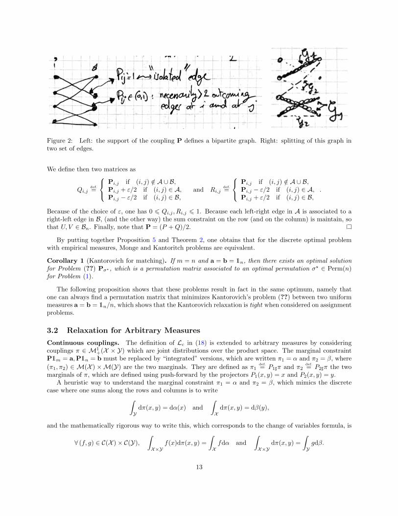
Figure 2: Left: the support of the coupling P defines a bipartite graph. Right: splitting of this graph intwo set of edges.

We define then two matrices as

Qi,jdef.=

Pi,j if (i, j) /∈ A ∪ B,Pi,j + ε/2 if (i, j) ∈ A,Pi,j − ε/2 if (i, j) ∈ B,

and Ri,jdef.=

Pi,j if (i, j) /∈ A ∪ B,Pi,j − ε/2 if (i, j) ∈ A,Pi,j + ε/2 if (i, j) ∈ B,

.

Because of the choice of ε, one has 0 6 Qi,j , Ri,j 6 1. Because each left-right edge in A is associated to aright-left edge in B, (and the other way) the sum constraint on the row (and on the column) is maintain, sothat U, V ∈ Bn. Finally, note that P = (P +Q)/2.

By putting together Proposition 5 and Theorem 2, one obtains that for the discrete optimal problemwith empirical measures, Monge and Kantoritch problems are equivalent.

Corollary 1 (Kantorovich for matching). If m = n and a = b = 1n, then there exists an optimal solutionfor Problem (??) Pσ? , which is a permutation matrix associated to an optimal permutation σ? ∈ Perm(n)for Problem (1).

The following proposition shows that these problems result in fact in the same optimum, namely thatone can always find a permutation matrix that minimizes Kantorovich’s problem (??) between two uniformmeasures a = b = 1n/n, which shows that the Kantorovich relaxation is tight when considered on assignmentproblems.

3.2 Relaxation for Arbitrary Measures

Continuous couplings. The definition of Lc in (18) is extended to arbitrary measures by consideringcouplings π ∈ M1

+(X × Y) which are joint distributions over the product space. The marginal constraintP1m = a,P1n = b must be replaced by “integrated” versions, which are written π1 = α and π2 = β, where

(π1, π2) ∈ M(X ) ×M(Y) are the two marginals. They are defined as π1def.= P1]π and π2

def.= P2]π the two

marginals of π, which are defined using push-forward by the projectors P1(x, y) = x and P2(x, y) = y.A heuristic way to understand the marginal constraint π1 = α and π2 = β, which mimics the discrete

case where one sums along the rows and columns is to write∫Y

dπ(x, y) = dα(x) and

∫X

dπ(x, y) = dβ(y),

and the mathematically rigorous way to write this, which corresponds to the change of variables formula, is

∀ (f, g) ∈ C(X )× C(Y),

∫X×Y

f(x)dπ(x, y) =

∫Xfdα and

∫X×Y

dπ(x, y) =

∫Ygdβ.

13

Using (4), these marginal constraints are also equivalent to imposing that π(A×Y) = α(A) and π(X ×B) =β(B) for sets A ⊂ X and B ⊂ Y.

In the general case, the mass conservation constraint (17) should thus rewritten as a marginal constrainton joint probability distributions

U(α, β)def.=π ∈M1

+(X × Y) ; π1 = α and π2 = β. (20)

The discrete case, when α =∑i aiδxi , β =

∑j ajδxj , the constraint π1 = α and π2 = β necessarily

imposes that π is discrete, supported on the set (xi, yj)i,j , and thus has the form π =∑i,j Pi,jδ(xi,yj).

The discrete formulation is thus a special case (and not some sort of approximation) of the continuousformulation.

Continuous Kantorovitch problem. The Kantorovich problem (18) is then generalized as

Lc(α, β)def.= min

π∈U(α,β)

∫X×Y

c(x, y)dπ(x, y). (21)

This is an infinite-dimensional linear program over a space of measures.On compact domain (X ,Y), (21) always has a solution, because using the weak-* topology (so called

weak topology of measures), the set of measure is compact, and a linear function with a continuous c(x, y)is weak-* continuous. And the set of constraint is non empty, taking α ⊗ β. On non compact domain, oneneeds to impose moment condition on α and β.

Probabilistic interpretation. If we denote X ∼ α the fact that the law of a random vector X is theprobability distribution α, then the marginal constraint appearing in (21) is simply that π is the law of acouple (X,Y ) and that its coordinates X and Y have laws α and β. The coupling π encodes the statisticaldependency between X and Y . For instance, π = α ⊗ β means that X and Y are independent, and itunlikely that such a coupling is optimal. Indeed as stated by Brenier’s theorem, optimal coupling for asquare Euclidean loss on contrary describe totally dependent variable.

With this remark, problem (21) reads equivalently

Lc(α, β) = minX×α,Y∼β

E(c(X,Y )). (22)

Monge-Kantorovitch equivalence. The proof of Brenier theorem 1 (detailed in Section 5.3) to provethe existence of a Monge map actually studies Kantorovitch relaxation, and proves that this relaxation istight in the sense that it has the same cost as Monge problem.

Indeed, if α has a density and we denote T = ∇ϕ the unique optimal transport, then the coupling

π = (Id, T )]α i.e. ∀h ∈ C(X × Y),

∫X×Y

hdπ =

∫Xh(x, T (x))dα(x)

is optimal. In term of random vector, denoting (X,Y ) a random vector with law π, it means that anysuch optimal random vector satisfies Y = T (X) where X ∼ α (and of course T (X) ∼ β by the marginalconstraint).

This key result is similar to Birkoff-von-Neumann Theorem 1 in the sense that it provides conditions en-suring the equivalence between Monge and Kantorovitch problems (note however that Birkoff-von-Neumanndoes not implies uniqueness). Note however that the settings are radically difference (one is fully discretewhile the other requires the sources to be “continuous”, i.e. to have a density).

14

3.3 Metric Properties

OT defines a distance. An important feature of OT is that it defines a distance between histogramsand probability measures as soon as the cost matrix satisfies certain suitable properties. Indeed, OT can beunderstood as a canonical way to lift a ground distance between points to a distance between histogram ormeasures.

Proposition 6. We suppose n = m, and that for some p > 1, C = Dp = (Dpi,j)i,j ∈ Rn×n where D ∈ Rn×n+

is a distance on JnK, i.e.

1. D ∈ Rn×n+ is symmetric;

2. Di,j = 0 if and only if i = j;

3. ∀ (i, j, k) ∈ JnK3,Di,k 6 Di,j + Dj,k.

ThenWp(a,b)

def.= LDp(a,b)1/p (23)

(note that Wp depends on D) defines the p-Wasserstein distance on Σn, i.e. Wp is symmetric, positive,Wp(a,b) = 0 if and only if a = b, and it satisfies the triangle inequality

∀a,a′,b ∈ Σn, Wp(a,b) 6 Wp(a,a′) + Wp(a

′,b).

Proof. Symmetry and definiteness of the distance are easy to prove: since C = Dp has a null diagonal,Wp(a,a) = 0, with corresponding optimal transport matrix P? = diag(a); by the positivity of all off-diagonalelements of Dp, Wp(a,b) > 0 whenever a 6= b (because in this case, an admissible coupling necessarily hasa non-zero element outside the diagonal); by symmetry of Dp, Wp(a,b) = 0 is itself a symmetric function.

To prove the triangle inequality of Wasserstein distances for arbitrary measures, [44, Theorem 7.3] usesthe gluing lemma, which stresses the existence of couplings with a prescribed structure. In the discretesetting, the explicit constuction of this glued coupling is simple. Let a,b, c ∈ Σn. Let P and Q be two

optimal solutions of the transport problems between a and b, and b and c respectively. We define bjdef.= bj

if bj > 0 and set otherwise bj = 1 (or actually any other value). We then define

Sdef.= P diag(1/b)Q ∈ Rn×n+ .

We remark that S ∈ U(a, c) because

S1n = P diag(1/b)Q1n = P(b/b) = P1Supp(b) = a

where we denoted 1Supp(b) the indicator of the support of b, and we use the fact that P1Supp(b) = P1 = b

because necessarily Pi,j = 0 for j /∈ Supp(b). Similarly one verifies that S>1n = c.

15

The triangle inequality follows from

Wp(a, c) =

(min

P∈U(a,c)〈P, Dp〉

)1/p

6 〈S, Dp〉1/p

=

∑ik

Dpik

∑j

PijQjk

bj

1/p

6

∑ijk

(Dij + Djk)p PijQjk

bj

1/p

6

∑ijk

Dpij

PijQjk

bj

1/p

+

∑ijk

Dpjk

PijQjk

bj

1/p

=

∑ij

DpijPij

∑k

Qjk

bj

1/p

+

∑jk

DpjkQjk

∑i

Pij

bj

1/p

=

∑ij

DpijPij

1/p

+

∑jk

DpjkQjk

1/p

= Wp(a,b) + Wp(b,b).

The first inequality is due to the suboptimality of S, the second is the usual triangle inequality for elementsin D, and the third comes from Minkowski’s inequality.

Proposition 6 generalizes from histogram to arbitrary measures that need not be discrete.

Proposition 7. We assume X = Y, and that for some p > 1, c(x, y) = d(x, y)p where d is a distance onX , i.e.

(i) d(x, y) = d(y, x) > 0;(ii) d(x, y) = 0 if and only if x = y;(ii) ∀ (x, y, z) ∈ X 3, d(x, z) 6 d(x, y) + d(y, z).

ThenWp(α, β)

def.= Ldp(α, β)1/p (24)

(note that Wp depends on d) defines the p-Wasserstein distance on X , i.e. Wp is symmetric, positive,Wp(α, β) = 0 if and only if α = β, and it satisfies the triangle inequality

∀ (α, β, γ) ∈M1+(X )3, Wp(α, γ) 6Wp(α, β) +Wp(β, γ).

This distance Wp defined though Kantorovitch problem (24) should be contrasted with the distance Wobtained using Monge’s problem (7). Kantorovitch distance is always finite, while Monge’s one might beinfinite if the constraint set T ; T]α = β is empty. In fact, one can show that as soon as this constraint

set is non-empty, and even if no optimal T exists, then one has Wp = Wp, which is a non-trivial result.Kantorovitch distance should thus be seen as a (convex) relaxation of Monge’s distance, which behave in amuch nicer way, as we will explore next (it is continuous with respect to the convergence in law topology.

Convergence in law topology. Let us first note that on a compact space, all Wp distance defines thesame topology (although they are not equivalent, the notion of converging sequence is the same).

Proposition 8. On a compact space X , one has for p 6 q

Wp(α, β) 6Wq(α, β) 6 diam(X )q−pq Wp(α, β)

qp

16

Proof. The left inequality follows from Jensen inequality, ϕ(∫c(x, y)dπ(x, y)) 6

∫ϕ(c(x, y))dπ(x, y), applied

to any probability distribution π and to the convex function ϕ(r) = rq/p to c(x, y) = ||x − y||p, so that onegets (∫

||x− y||pdπ(x, y)

) qp

6∫||x− y||qdπ(x, y).

The right inequality follows from||x− y||q 6 diam(X )q−p||x− y||p.

The Wasserstein distance Wp has many important properties, the most important one being that it is aweak distance, i.e. it allows to compare singular distributions (for instance discrete ones) and to quantifyspatial shift between the supports of the distributions. This corresponds to the notion of weak∗ convergence.

Definition 2 (Weak∗ topology). (αk)k converges weakly∗ to α in M1+(X ) (denoted αk α) if and only if

for any continuous function f ∈ C(X ),∫X fdαk →

∫X fdα.

In term of random vectors, if Xn ∼ αn and X ∼ α (not necessarily defined on the same probabilityspace), the weak∗ convergence corresponds to the convergence in law of Xn toward X.

Definition 3 (Strong topology). The simplest distance on Radon measures is the total variation norm,which is the dual norm of the L∞ norm on C(X ) and whose topology is often called the “strong” topology

||α− β||TV def.= sup||f ||∞61

∫fd(α− β) = |α− β|(X )

where |α − β|(X ) is the mass of the absolute value of the difference measure. When α − β = ρdx has adensity, then ||α− β||TV =

∫|ρ(x)|dx = ||ρ||L1(dx) is the L1 norm associated to dx. When α− β =

∑i uiδzi

is discrete, then ||α− β||TV =∑i |ui| = ||u||`1 is the discrete `1 norm.

In the special case of Diracs, having∫fdδxn = f(xn)→

∫fdδx = f(x) for any continuous f is equivalent

to xn → x. One can then contrast the strong topology with the Wasserstein distance, if xn 6= x,

||δxn − δx||TV = 2 and Wp(δxn , δx) = d(xn, x).

This shows that for the strong topology, Diracs never converge, while they do converge for the Wassersteindistance. In fact it is a powerful property of the Wasserstein distance, which is regular with respect to theweak∗ topology, and metrizes it.

Proposition 9. If X is compact, αk α if and only if Wp(αk, α)→ 0.

The proof of this proposition requires the use of duality, and is delayed to later, see Proposition 2. Onnon-compact spaces, one needs also to impose the convergence of the moments up to order p. Note that thereexists alternative distances which also metrize weak convergence. The simplest one are Hilbertian kernelnorms, which are detailed in Section 6.3.

Applications and implications Applications for having a geometric distance : barycenters, shape reg-istration loss functions, density fitting

4 Sinkhorn

4.1 Entropic Regularization for Discrete Measures

Relative entropy The Kullback-Leibler divergence is defined as

KL(P|Q)def.=∑i,j

Pi,j log

(Pi,j

Qi,j

)−Pi,j + Qi,j . (25)

17

with the convention 0 log(0) = 0 and KL(P|Q) = +∞ if there exists some (i, j) such that Qi,j = 0 butPi,j 6= 0. The special case KL(P|1) corresponds to minus the Shannon-Boltzmann entropy. The functionKL(·|Q) is strongly convex, because its hessian is ∂2KL(P|Q) = diag(1/Pi,j) and Pi,j 6 1.

KL is a particular instance (and actually the unique case) of both a ϕ-divergence (as defined in Section ??)and a Bregman divergence. This unique property is at the heart of the fact that this regularization leads toelegant algorithms and a tractable mathematical analysis. One thus has KL(P|Q) > 0 and KL(P|Q) = 0if and only if P = Q.

Entropic Regularization for Discrete Measures. The idea of the entropic regularization of optimaltransport is to use KL as a regularizing function to obtain approximate solutions to the original transportproblem (??):

LεC(a,b)def.= min

P∈U(a,b)〈P, C〉+ εKL(P|a⊗ b). (26)

Here we used as a reference measure for the relative entropy a⊗b = (aibj)i,j . This choice of normalization,specially in this discrete setting, has no importance for the selection of the optimal P since it only affectsthe objective by a constant, indeed for P ∈ U(a,b), one has

KL(P|a⊗ b) = KL(P|a′ ⊗ b′) + KL(a′ ⊗ b′|a⊗ b)

[ToDo: check this]. This choice of normalization is however important to deal with situation where thesupport of a and b can change, and in particular when later we will deal with possibly continuous distribution.It also affect the values of the cost LεC(a,b) and this normalization will be instrumental to define a properSinkhorn divergence.

Smoothing effect. Since the objective is a ε-strongly convex function, problem 26 has a unique optimalsolution. As studied in Section ??, this smoothing, beyond providing uniqueness, actually leads to LεC(a,b)being a smooth function of a,b and C. The effect of the entropy is to act as a barrier function for thepositivity constraint. As we will show next, this forces the solution P to be strictly positive on the supportof a⊗ b.

One has the following convergence property.

Proposition 10 (Convergence with ε). The unique solution Pε of (26) converges to the optimal solutionwith maximal entropy within the set of all optimal solutions of the Kantorovich problem, namely

Pεε→0−→ argmin

PKL(P|a⊗ b) ; P ∈ U(a,b), 〈P, C〉 = LC(a,b) (27)

so that in particular

LεC(a,b)ε→0−→ LC(a,b).

One hasPε

ε→∞−→ a⊗ b. (28)

Proof. Case ε→ 0. We consider a sequence (ε`)` such that ε` → 0 and ε` > 0. We denote P` the solutionof (26) for ε = ε`. Since U(a,b) is bounded, we can extract a sequence (that we do not relabel for sakeof simplicity) such that P` → P?. Since U(a,b) is closed, P? ∈ U(a,b). We consider any P such that〈C, P〉 = LC(a,b). By optimality of P and P` for their respective optimization problems (for ε = 0 andε = ε`), one has

0 6 〈C, P`〉 − 〈C, P〉 6 ε`(KL(P`|a⊗ b)−KL(P|a⊗ b)). (29)

Since H is continuous, taking the limit `→ +∞ in this expression shows that 〈C, P?〉 = 〈C, P〉 so that P? isa feasible point of (27). Furthermore, dividing by ε` in (29) and taking the limit shows that KL(P|a⊗b) 6KL(P?|a ⊗ b), which shows that P? is a solution of (27). Since the solution P?

0 to this program is uniqueby strict convexity of KL(·|a⊗ b), one has P? = P?

0, and the whole sequence is converging.

18

Case ε→ +∞. Evaluating at a⊗ b the energy, one has

〈C, Pε〉+ εKL(Pε|α⊗ β) 6 〈C, α⊗ β〉+ ε× 0

and since 〈C, Pε〉 > 0, this leads to

KL(Pε|α⊗ β) 6 ε−1〈C, α⊗ β〉 6 ||C||∞ε

so that KL(Pε|α⊗ β)→ 0 and thus Pε → α⊗ β since KL is a valid divergence.

4.2 General Formulation

One can consider arbitrary measures by replacing the discrete entropy by the relative entropy with respect

to the product measure dα⊗ dβ(x, y)def.= dα(x)dβ(y), and propose a regularized counterpart to (21) using

Lεc(α, β)def.= min

π∈U(α,β)

∫X×Y

c(x, y)dπ(x, y) + εKL(π|α⊗ β) (30)

where the relative entropy is a generalization of the discrete Kullback-Leibler divergence (25)

KL(π|ξ) def.=

∫X×Y

log(dπ

dξ(x, y)

)dπ(x, y) +

∫X×Y

(dξ(x, y)− dπ(x, y)), (31)

and by convention KL(π|ξ) = +∞ if π does not have a density dπdξ with respect to ξ. It is important to realize

that the reference measure α⊗β chosen in (30) to define the entropic regularizing term KL(·|α⊗β) plays nospecific role, only its support matters. This problem is often referred to as the “static Schrodinger problem”,since π is intended to model the most likely coupling between particules of gaz which can be only observedat two different times (it is the so-called lazy gaz model). The parameter ε controls the temperature of thegaz, and particules do not move in deterministic straight line as in optimal transport for the Euclidean cost,but rather according to a stochastic Brownian bridge.

Remark 3 (Probabilistic interpretation). If (X,Y ) ∼ π have marginalsX ∼ α and Y ∼ β, then KL(π|α⊗β) =I(X,Y ) is the mutual information of the couple, which is 0 if and only if X and Y are independent. Theentropic problem (30) is thus equivalent to

min(X,Y ),X∼α,Y∼β

E(c(X,Y )) + εI(X,Y ).

Using a large ε thus enforces the optimal coupling to describe independent variables, while, according toBrenier’s theorem, small ε rather imposes a deterministic dependency between the couple according to aMonge map.

4.3 Sinkhorn’s Algorithm

The following proposition shows that the solution of (26) has a specific form, which can be parameterizedusing n+m variables. That parameterization is therefore essentially dual, in the sense that a coupling P inU(a,b) has nm variables but n+m constraints.

Proposition 11. P is the unique solution to (26) if and only if there exists (u,v) ∈ Rn+ × Rm+ such that

∀ (i, j) ∈ JnK× JmK, Pi,j = uiKi,jvj (32)

and P ∈ U(a, β).

19

Proof. Introducing two dual variables f ∈ Rn,g ∈ Rm for each marginal constraint, the Lagrangian of (26)reads

E(P, f,g) = 〈P, C〉+ εKL(P|a⊗ b) + 〈f, a−P1m〉+ 〈g, b−PT1n〉.Considering first order conditions (where we ignore the positivity constraint, which can be made rigorous byshowing the associated multiplier vanishes), we have

∂E(P, f,g)

∂Pi,j= Ci,j + ε log

(Pi,j

aibj

)− fi − gj = 0.

which results, for an optimal P coupling to the regularized problem, in the expression Pi,j = aibjefi+gj−Ci,j

ε

which can be rewritten in the form provided in the proposition using non-negative vectors udef.= (aie

fi/ε)iand v

def.= (bje

gj/ε)j .

The factorization of the optimal solution exhibited in Equation (32) can be conveniently rewritten inmatrix form as P = diag(u)K diag(v). u,v must therefore satisfy the following non-linear equations whichcorrespond to the mass conservation constraints inherent to U(a,b),

diag(u)K diag(v)1m = a, and diag(v)K> diag(u)1n = b, (33)

These two equations can be further simplified, since diag(v)1m is v, and the multiplication of diag(u) timesKv is

u (Kv) = a and v (KTu) = b (34)

where corresponds to entry-wise multiplication of vectors. That problem is known in the numerical analysiscommunity as the matrix scaling problem (see [35] and references therein). An intuitive way to try to solvethese equations is to solve them iteratively, by modifying first u so that it satisfies the left-hand side ofEquation (34) and then v to satisfy its right-hand side. These two updates define Sinkhorn’s algorithm

u(`+1) def.=

a

Kv(`)and v(`+1) def.

=b

KTu(`+1), (35)

initialized with an arbitrary positive vector, for instance v(0) = 1m. The division operator used abovebetween two vectors is to be understood entry-wise. Note that a different initialization will likely lead to adifferent solution for u,v, since u,v are only defined up to a multiplicative constant (if u,v satisfy (33) thenso do λu,v/λ for any λ > 0). It turns out however that these iterations converge, as we detail next.

[ToDo: Say a few word about the general probleme of scaling a matrix to a bistochasticone, and why this is non trivial for matrices with vanishing entries.]

A chief advantage, beside its simplicity, of Sinkhorn’s algorithm is that the only computationnaly expen-sive step are matrix-vector multiplication by the Gibbs kernel, so that its complexity scales likes Knm whereK is the number of Sinkhorn iteration, which can be kept polynomially in 1/ε if one is interested in reachingan accuracy ε on the (unregularized) transportation cost. Note however that in many situation, one is notinterested in reaching high accuracy, because targeted application success is often only remotely connected tothe ability to solve an optimal transport problem (but rather only being able to compare in a geometricallyfaithful way distribution), so that K is usually quite small. This should be contrasted with interior pointmethods, which also operate by introducing a barrier function of the form −∑i log(Pi,j). These algorithmhave typically a complexity of the order O(n6 log(|ε|)) [ToDo: check].

The second crucial aspect of Sinkhorn is that matrix-vector multiplication streams extremely well onGPU. Even better, if one is interested in computing many OT problem with a fixed cost matrix C, one canreplace many matrix-vector multiplication by matrix-matrix multiplication, so that the computation gain isenormous.

20

4.4 Convergence

Convergence finite dimension via alternating projections. One has

〈P, C〉+ εKL(P|a⊗ b) = εKL(P|K) + cst,

so that the unique solution Pε of (26) is a projection onto U(a,b) of the Gibbs kernel K

Pε = ProjKLU(a,b)(K)

def.= argmin

P∈U(a,b)

KL(P|K). (36)

Denoting

C1a

def.= P ; P1m = a and C2

bdef.=

P ; PT1m = b

the rows and columns constraints, one has U(a,b) = C1a∩C2

b. One can use Bregman iterative projections [11]

P(`+1) def.= ProjKL

C1a (P(`)) and P(`+2) def.= ProjKL

C2b(P(`+1)). (37)

Since the sets C1a and C2

b are affine, these iterations are known to converge to the solution of (36), see [11].The two projector are simple to compute since they corresponds to scaling respectively the rows and the

columns

ProjKLC1a (P) = diag

(a

P1m

)P and ProjKL

C2b(P) = P diag

(b

P>1n

).

These iterate are equivalent to Sinkhorn iterations (35) since defining

P(2`) def.= diag(u(`))K diag(v(`)),

one has

P(2`+1) def.= diag(u(`+1))K diag(v(`))

and P(2`+2) def.= diag(u(`+1))K diag(v(`+1))

In practice however one should prefer using (35) which only requires manipulating scaling vectors andmultiplication against a Gibbs kernel, which can often be accelerated (see below Remarks ?? and ??).

Such a convergence analysis using Bregman projection is however of limited interested because it onlyworks in finite dimension. For instance, the linear convergence speed one can obtain with these analyses(because the objective is strongly convex) will degrade with the dimension (and of course also with ε). Itis also possible to decay ε during the iterates to improve the speed and rely on multiscale strategies in lowdimension.

Convergence for the Hilbert metric As initially explained by [26], the global convergence analysis ofSinkhorn is greatly simplified using Hilbert projective metric on Rn+,∗ (positive vectors), defined as

∀ (u,u′) ∈ (Rn+,∗)2, dH(u,u′)

def.= || log(u)− log(v)||V

where the variation semi-norm is||z||V = max(z)−min(z).

One can show that dH is a distance on the projective cone Rn+,∗/ ∼, where u ∼ u′ means that ∃s > 0,u = su′

(the vector are equal up to rescaling, hence the naming “projective”), and that (Rn+,∗/ ∼, dH) is then acomplete metric space. It was introduced independently by [8] and [39] to provide a quantitative proof ofPerron-Frobenius theorem (convergence of iterations of positive matrices). Sinkhorn should be thought as anon-linear generalization of Perron-Frobenius.

21

Theorem 3. Let K ∈ Rn×m+,∗ , then for (v,v′) ∈ (Rm+,∗)2

dH(Kv,Kv′) 6 λ(K)dH(v,v′) where

λ(K)

def.=

√η(K)−1√η(K)+1

< 1

η(K)def.= max

i,j,k,`

Ki,kKj,`

Kj,kKi,`.

The following theorem, proved by [26], makes use of this Theorem 3 to show the linear convergence ofSinkhorn’s iterations.

Theorem 4. One has (u(`),v(`))→ (u?,v?) and

dH(u(`),u?) = O(λ(K)2`), dH(v(`),v?) = O(λ(K)2`). (38)

One also has

dH(u(`),u?) 6dH(P(`)1m,a)

1− λ(K)and dH(v(`),v?) 6

dH(P(`),>1n,b)

1− λ(K), (39)

where we denoted P(`) def.= diag(u(`))K diag(v(`)). Lastly, one has

‖ log(P(`))− log(P?)‖∞ 6 dH(u(`),u?) + dH(v(`),v?) (40)

where P? is the unique solution of (26).

Proof. One notice that for any (v,v′) ∈ (Rm+,∗)2, one has

dH(v,v′) = dH(v/v′,1m) = dH(1m/v,1m/v′).

This shows that

dH(u(`+1),u?) = dH

( a

Kv(`),

a

Kv?

)= dH(Kv(`),Kv?) 6 λ(K)dH(v(`),v?).

where we used Theorem 3. This shows (38). One also has, using the triangular inequality

dH(u(`),u?) 6 dH(u(`+1),u(`)) + dH(u(`+1),u?) 6 dH

( a

Kv(`),u(`)

)+ λ(K)dH(u(`),u?)

= dH

(a,u(`) (Kv(`))

)+ λ(K)dH(u(`),u?),

which gives the first part of (39) since u(`) (Kv(`)) = P(`)1m (the second one being similar). The proofof (40) follows from [26, Lemma 3]

The bound (39) shows that some error measures on the marginal constraints violation, for instance

‖P(`)1m − a‖1 and ‖P(`)T1n − b‖1, are useful stopping criteria to monitor the convergence. This theorem

shows that Sinkhorn algorithm converges linearly, but the rates becomes exponentially bad as ε→ 0, since itscales like e−1/ε. In practice, one eventually observes a linear rate after enough iteration, because the locallinear rate is much better, usually of the order 1− ε.

5 Dual Problem

5.1 Discrete dual

The Kantorovich problem (??) is a linear program, so that one can equivalently compute its value bysolving a dual linear program.

22

Proposition 12. One hasLC(a,b) = max

(f,g)∈R(a,b)〈f, a〉+ 〈g, b〉 (41)

where the set of admissible potentials is

R(a,b)def.= (f,g) ∈ Rn × Rm ; ∀ (i, j) ∈ JnK× JmK, f⊕ g 6 C (42)

Proof. For the sake of completeness, let us derive this dual problem with the use of Lagrangian duality. TheLagangian associate to (??) reads

minP>0

max(f,g)∈Rn×Rm

〈C, P〉+ 〈a−P1m, f〉+ 〈b−P>1n, g〉. (43)

For linear program, if the primal set of constraint is non-empty, one can always exchange the min and themax and get the same value of the linear program, and one thus consider

max(f,g)∈Rn×Rm

〈a, f〉+ 〈b, g〉+ minP>0〈C− f1>m − 1ng>, P〉.

We conclude by remarking that

minP>0〈Q, P〉 =

0 if Q > 0−∞ otherwise

so that the constraint reads C− f1>m − 1ng> = C− f⊕ g > 0.

The primal-dual optimality relation for the Lagrangian (43) allows to locate the support of the optimaltransport plan

Supp(P) ⊂

(i, j) ∈ JnK× JmK ; fi + gj = Ci,j

. (44)

The formulation (70) shows that (a,b) 7→ LC(a,b) is a convex function (as a supremum of linearfunctions). From the primal problem (??), one also sees that C 7→ LC(a,b) is concave.

5.2 General formulation

To extend this primal-dual construction to arbitrary measures, it is important to realize that measures

are naturally paired in duality with continuous functions, using the pairing 〈f, α〉 def.=∫fdα.

Proposition 13. One has

Lc(α, β) = max(f,g)∈R(c)

∫Xf(x)dα(x) +

∫Yg(y)dβ(y), (45)

where the set of admissible dual potentials is

R(c)def.= (f, g) ∈ C(X )× C(Y) ; ∀(x, y), f(x) + g(y) 6 c(x, y) . (46)

Here, (f, g) is a pair of continuous functions, and are often called “Kantorovich potentials”.

The discrete case (70) corresponds to the dual vectors being samples of the continuous potentials, i.e.(fi,gj) = (f(xi), g(yj)). The primal-dual optimality conditions allow to track the support of optimal plan,and (44) is generalized as

Supp(π) ⊂ (x, y) ∈ X × Y ; f(x) + g(y) = c(x, y) . (47)

Note that in contrast to the primal problem (21), showing the existence of solutions to (45) is non-trivial, because the constraint set R(c) is not compact and the function to minimize non-coercive. Using themachinery of c-transform detailed in Section ??, one can however show that optimal (f, g) are necessarilyLipschitz regular, which enable to replace the constraint by a compact one.

23

5.3 c-transforms

Definition. Keeping a dual potential g fixed, one can try to minimize in closed form the dual problem (45),which leads to consider

supg∈C(Y)

∫gdβ ; ∀ (x, y), g(y) 6 c(x, y)− f(x)

.

The constraint can be replaced by∀ y ∈ Y, g(y) 6 f c(y)

where we define the c-transform as

∀ y ∈ Y, f c(y)def.= inf

x∈Xc(x, y)− f(x). (48)

Since β is positive, the maximization of∫gdβ is thus achieved at those functions such that g = f c on the

support of β, which means β-almost everywhere.Similarly, we defined the c-transform, which a transform for the symetrized cost c(y, x) = c(x, y), i.e.

∀x ∈ X , gc(x)def.= inf

y∈Yc(x, y)− g(y),

and one checks that any function f such that f = gc α-almost everywhere is solution to the dual problemfor a fixed g.

The map (f, g) ∈ C(X ) × C(Y) 7→ (gc, f c) ∈ C(X ) × C(Y) replaces dual potentials by “better” ones(improving the dual objective E). Functions that can be written in the form f c and gc are called c-concaveand c-concave functions.

Note that these partial minimizations define maximizers on the support of respectively α and β, whilethe definitions (48) actually define functions on the whole spaces X and Y. This is thus a way to extend ina canonical way solutions of (45) on the whole spaces.

Furthermore, if c is Lipschitz, then f c and gc are also Lipschitz functions, as we now show. This propertyis crucial to show existence of solution to the dual problem. Indeed, since one can impose this Lipschitz onthe dual problems, the constraint set is compact via Ascoli theorem.

Proposition 14. If c is L-Lipschitz with respect to the second variable, then f c is L-Lipschitz.

Proof. We apply to Fx = c(x, ·)−f(x) the fact that if all the Fx are L-Lipschitz, then the Lipschitz constantof F = minx Fx is L. Indeed, using the fact that | inf(A)− inf(B)| 6 sup |A−B| for two function A and B,then

|F (y)− F (y′)| = | infx

(Fx(y))− infx

(Fx(y′))| 6 supx|Fx(y)− Fx(y′)| 6 sup

xLd(y, y′) = Ld(y, y′).

Euclidean case. The special case c(x, y) = −〈x, y〉 in X = Y = Rd is of utmost importance because itallows one to study the W2 problem, since for any π ∈ U(α, β)∫

||x− y||2dπ(x, y) = cst− 2

∫〈x, y〉dπ(x, y) where cst =

∫||x||2dα(x) +

∫||y||2dβ(y).

For this special choice of cost, one has f c = −(−f)∗ where h∗ is the Fenchel-Legendre transform

h∗(y)def.= sup

x〈x, y〉 − h(y).

One has that h∗ is always convex, so that f c is always concave. For a general cost, one thus denotes functionsof the form f c as being c-concave.

24

The failure of alternate optimization. A crucial property of the Legendre transform is that f∗∗∗ = f∗,and that f∗∗ is the convex enveloppe of f (the largest convex function bellow f). These properties carriesover for the more general setting of c-transforms.

Proposition 15. The following identities, in which the inequality sign between vectors should be understood

elementwise, hold, denoting f ccdef.= (f c)c:

(i) f 6 f ′ ⇒ f c > f ′c,

(ii) f cc > f ,

(iii) gcc > g,

(iv) f ccc = f c.

Proof. The first inequality (i) follows from the definition of c-transforms. To prove (ii), expanding thedefinition of f cc we have(

f cc)

(x) = minyc(x, y)− f c(y) = min

yc(x, y)−min

x′(c(x′, y)− f(x′)).

Now, since −minx′ c(x′, y)− f(x′) > −(c(x, y)− f(x)), we recover

(f cc)(x) > minyc(x, y)− c(x, y) + f(x) = f(x).

The relation gcc > g is obtained in the same way. Now, to prove (iv), we first apply (ii) and then (i) withf ′ = f cc to have f c > f cc. Then we apply (iii) to g = f c to obtain f c 6 f ccc.

This invariance property shows that one can “improve” only once the dual potential this way. Indeed,starting from any pair (f, g), one obtains the following iterates by alternating maximization

(f, g) 7→ (f, f c) 7→ (f cc, f c) 7→ (f cc, f ccc) = (f cc, f c) . . . (49)

so that one reaches a stationary point. This failure is the classical behavior of alternating maximizationon a non-smooth problem, where the non-smooth part of the functional (here the constraint) mixes thetwo variables. The workaround is to introduce a smoothing, which is the classical method of augmentedLagrangian, and that we will develop here using entropic regularization, and corresponds to Sinkhorn’salgorithm.

6 Semi-discrete and W1

6.1 Semi-discrete

A case of particular interest is when β =∑j bjδyj is discrete (of course the same construction applies if

α is discrete by exchanging the role of α, β). One can adapt the definition of the c transform (48) to thissetting by restricting the minimization to the support (yj)j of β,

∀g ∈ Rm, ∀x ∈ X , gc(x)def.= min

j∈JmKc(x, yj)− gj . (50)

This transform maps a vector g to a continuous function gc ∈ C(X ). Note that this definition coincideswith (48) when imposing that the space X is equal to the support of β.

Crucially, using the discrete c-transform, when β is a discrete measure, yields a finite-dimensional opti-mization,

Lc(α, β) = maxg∈Rm

E(g)def.=

∫X

gc(x)dα(x) +∑j

gjbj . (51)

25

The Laguerre cells associated to the dual weights g

Lj(g)def.=x ∈ X ; ∀ j′ 6= j, c(x, yj)− gj 6 c(x, yj′)− gj′

induce a disjoint decomposition of X =

⋃j Lj(g). When g is constant, the Laguerre cells decomposition

corresponds to the Voronoi diagram partition of the space.This allows one to conveniently rewrite the minimized energy as

E(g) =

m∑j=1

∫Lj(g)

(c(x, yj)− gj

)dα(x) + 〈g, b〉. (52)

The following proposition provides a formula for the gradient of this convex function.

Proposition 16. If α has a density with respect to Lebesgue measure and if c is smooth away from thediagonal, then E is differentiable and

∀ j ∈ JmK, ∇E(g)j = bj −∫

Lj(g)

dα.

Proof. One has

E(g + εδj)− E(g)− ε(

bj −∫

Lj(g)

dα

)=∑k

∫Lk(g+εδj)

c(x, xk)dα(x)−∫

Lk(g)

c(x, xk)dα(x).

Most of the terms in the right hand side vanish (because most the Laguerre cells associated to g+εδj are equalto those of g) and the only terms remaining correspond to neighboring cells (j, k) such that Lj(g)∩Lk(g) 6= ∅(for the cost ||x − y||2 and g = 0 this forms the Delaunay triangulation). On these pairs, the right integraldiffers on a volume of the order of ε (since α has a density) and the function being integrated only varies onthe order of ε (since the cost is smooth). So the right hand side is of the order of ε2.

The first order optimality condition shows that in order to solve the dual semi discrete problem, oneneeds to select the weights g in order to drive the Laguerre cell in a configuration such that

∫Lj(g)

dα = bj ,

i.e. each cell should capture the correct amount of mass. In this case, the optimal transport T such thatT]α = β (which exists and is unique according to Brenier’s theorem if α has a density) is piecewise constantand map x ∈ Lj(g) to yj .

In the special case c(x, y) = ||x − y||2, the decomposition in Laguerre cells is also known as a “powerdiagram”. In this case, the cells are polyhedral and can be computed efficiently using computational geometryalgorithms; see [3]. The most widely used algorithm relies on the fact that the power diagram of points inRd is equal to the projection on Rd of the convex hull of the set of points ((yj , ||yj ||2−gj))

mj=1 ⊂ Rd+1. There

are numerous algorithms to compute convex hulls; for instance, that of [18] in two and three dimensions hascomplexity O(m log(Q)), where Q is the number of vertices of the convex hull.

Stochastic optimization. The semidiscrete formulation (52) is also appealing because the energies to beminimized are written as an expectation with respect to the probability distribution α,

E(g) =

∫XE(g, x)dα(x) = EX(E(g, X)) where E(g, x)

def.= gc(x)− 〈g, b〉,

and X denotes a random vector distributed on X according to α. Note that the gradient of each of theinvolved functional reads

∇gE(x,g) = (1Lj(g)(x)− bj)mj=1 ∈ Rm

where 1Lj(g) is the indicator function of the Laguerre cell. One can thus use stochastic optimization methodsto perform the maximization, as proposed in [27]. This allows us to obtain provably convergent algorithms

26

without the need to resort to an arbitrary discretization of α (either approximating α using sums of Diracsor using quadrature formula for the integrals). The measure α is used as a black box from which one candraw independent samples, which is a natural computational setup for many high-dimensional applicationsin statistics and machine learning.

Initializing g(0) = 0m, the stochastic gradient descent algorithm (SGD; used here as a maximizationmethod) draws at step ` a point x` ∈ X according to distribution α (independently from all past and futuresamples (x`)`) to form the update

g(`+1) def.= g(`) + τ`∇gE(g(`), x`). (53)

The step size τ` should decay fast enough to zero in order to ensure that the “noise” created by using∇gE(x`,g) as a proxy for the true gradient ∇E(g) is canceled in the limit. A typical choice of schedule is

τ`def.=

τ01 + `/`0

, (54)

where `0 indicates roughly the number of iterations serving as a warmup phase. One can prove the conver-gence result

E(g?)− E(E(g(`))) = O

(1√`

),

where g? is a solution of (??) and where E indicates an expectation with respect to the i.i.d. sampling of(x`)` performed at each iteration.

Optimal quantization. The optimal quantization problem of some measure α corresponds to the resolu-tion of

Qm(α) = minY=(yj)mj=1,(bj)

mj=1

Wp(α,∑j

bjδyj ).

This problem is at the heart of the computation of efficient vector quantizer in information theory andcompression, and is also the basic problem to solve for clustering in unsupervised learning. The asymptoticbehavior of Qm is of fundamental importance, and its precise behavior is in general unknown. For a measurewith a density in Euclidean space, it scales like O(1/n1/d), so that quantization generally suffers from thecurse of dimensionality.

This optimal quantization problem is convex with respect to b, but is unfortunately non-convex withrespect to Y = (yj)j . Its resolution is in general NP-hard. The only setting where this problem is simpleis the 1-D case, in which case the optimal sampling is simply yj = C−1

α (j/m). [ToDo: see where this isproved]

Solving explicitly for the minimization over b in the formula (51) (exchanging the role of the min and themax) shows that necessarily, at optimality, one has g = 0, so that the optimal transport maps the Voronoicells Lj(g = 0), which we denote Vj(Y ) to highlight the dependency on the quantization points Y = (yj)j

Vj(Y ) = x ; ∀ j′, c(x, yj′) 6 c(x, yj) .

This also shows that the quantization energy can be rewritten in a more intuitive way, which accounts forthe average quantization error induced by replacing a point x by its nearest centroid

Qm(α) = minYF(Y )

def.=

∫X

min16j6m

c(x, yj)dα(x).

At any local minimizer (at least if α has a density so that this function is differentiable) of this energy overY , one sees that each yj should be a centroid of its associated Voronoi region,

yj ∈ argminy

∫Vj(Y )

c(x, y)dα(x).

27

For instance, when c(x, y) = ||x−y||2, one sees that any local minimizer should satisfy the fixed point equation

yj =

∫Vj(Y )

xdα(x)∫Vj(Y )

dα.

The celebrated k-means algorithm, also known as Lloyd algorithm, iteratively apply this fixed point. It isnot guaranteed to converge (it could in theory cycle) but in practice it always converge to a local minimum.A practical issue to obtain a good local minimizer is to seed a good initial configuration. The intuitive wayto achieve this is to spread them as much as possible, and a well known algorithm to do so is the k-means++methods, which achieve without even any iteration a quantization cost which is of the order of log(m)Qm(α).

6.2 W1

c-transform for W1. Here we assume that d is a distance on X = Y, and we solve the OT problem withthe ground cost c(x, y) = d(x, y). The following proposition highlights key properties of the c-transform (48)in this setup. In the following, we denote the Lipschitz constant of a function f ∈ C(X ) as

Lip(f)def.= sup

|f(x)− f(y)|d(x, y)

; (x, y) ∈ X 2, x 6= y

.

Proposition 17. Suppose X = Y and c(x, y) = d(x, y). Then, there exists g such that f = gc if and onlyLip(f) 6 1. Furthermore, if Lip(f) 6 1, then f c = −f .

Proof. First, suppose f = gc for some g. Then, for x, y ∈ X ,

|f(x)− f(y)| =∣∣∣∣ infz∈X

d(x, z)− g(z) − infz∈X

d(y, z)− g(z)

∣∣∣∣6 supz∈X|d(x, z)− d(y, z)| 6 d(x, y).

The first equality follows from the definition of gc, the next inequality from the identity | inf f − inf g| 6sup |f − g|, and the last from the triangle inequality. This shows that Lip(f) 6 1.

If f is 1-Lipschitz, for all x, y ∈ X , f(y)− d(x, y) 6 f(x) 6 f(y) + d(x, y), which shows that

f c(y) = infx∈X

[d(x, y)− f(x)] > infx∈X

[d(x, y)− f(y)− d(x, y)] = −f(y),

f c(y) = infx∈X

[d(x, y)− f(x)] 6 infx∈X

[d(x, y)− f(y) + d(x, y)] = −f(y),

and thus f c = −f .Applying this property to −f which is also 1-Lipschitz shows that (−f)c = f so that f is indeed c-concave

(i.e. it is the c-transform of a function).

Using the iterative c-transform scheme (49), one can replace the dual variable (f, g) by (f cc, f c) =(−f c, fc), or equivalently by any pair (f,−f) where f is 1-Lipschitz. This leads to the following alternativeexpression for the W1 distance

W1(α, β) = maxf

∫Xfd(α− β) ; Lip(f) 6 1

. (55)

This expression shows that W1 is actually a norm, i.e.W1(α, β) = ||α − β||W1, and that it is still valid for

any measures (not necessary positive) as long as∫X α =

∫X β. This norm is often called the Kantorovich-

Rubinstein norm [33].

28

For discrete measures of the form (2), writing α − β =∑k mkδzk with zk ∈ X and

∑k mk = 0, the

optimization (55) can be rewritten as

W1(α, β) = max(fk)k

∑k

fkmk ; ∀ (k, `), |fk − f`| 6 d(zk, z`),

(56)

which is a finite-dimensional convex program with quadratic-cone constraints. It can be solved using interiorpoint methods or, as we detail next for a similar problem, using proximal methods.

When using d(x, y) = |x− y| with X = R, we can reduce the number of constraints by ordering the zk’svia z1 6 z2 6 . . .. In this case, we only have to solve

W1(α, β) = max(fk)k

∑k

fkmk ; ∀ k, |fk+1 − fk| 6 zk+1 − zk,

which is a linear program. Note that furthermore, in this 1-D case, a closed form expression for W1 usingcumulative functions is given in (12).

W1 on Euclidean spaces In the special case of Euclidean spaces X = Y = Rd, using c(x, y) = ||x − y||,the global Lipschitz constraint appearing in (55) can be made local as a uniform bound on the gradient off ,

W1(α, β) = supf

∫Rdf(dα− dβ) ; ||∇f ||∞ 6 1

. (57)

Here the constraint ||∇f ||∞ 6 1 signifies that the norm of the gradient of f at any point x is upper boundedby 1, ||∇f(x)||2 6 1 for any x.

Considering the dual problem to (57), denoting ξdef.= α− β, and using that

ι||·||Rd61(u) = maxv〈u, v〉 − ||v||Rd

one has a maximization on flow vector fields s : Rd → Rd

W1(α, β) = supf

infs(x)∈Rd

∫Rdfdξ −

∫〈∇f(x), s(x)〉dx+

∫||s(x)||Rddx

= infs(x)∈Rd

∫||s(x)||dx+ sup

f

∫f(x)(dξ − div(s)dx)

one obtains an optimization problem under fixed divergence constraint

W1(α, β) = infs

∫Rd||s(x)||Rddx ; div(s) = α− β

, (58)

which is often called the Beckmann formulation [5]. Here the vectorial function s(x) ∈ R2 can be interpretedas a flow field, describing locally the movement of mass. Outside the support of the two input measures,div(s) = 0, which is the conservation of mass constraint. Once properly discretized using finite elements,Problems (57) and (58) become a nonsmooth convex optimization problems.

The previous formulations (57) and (58) ofW1 can be generalized to the setting where X is a Riemannianmanifold, i.e. c(x, y) = d(x, y) where d is the associated geodesic distance (and then for smooth manifolds,the gradient and divergence should be understood as the differential operators on manifold). In a similarway it can be extended on a graph (where the geodesic distance is the length of the shortest path), in thiscase, the gradient and divergence are the corresponding finite difference operations operating along the edgesof the graph. In this setting, the corresponding linear program can be solved using a min-cost flow simplexin complexity O(n2 log(n)) for sparse graph (e.g. grids).

29

6.3 Dual norms (Integral Probability Metrics)

Formulation (57) is a special case of a dual norm. A dual norm is a convenient way to design “weak”norms that can deal with arbitrary measures. For a symmetric convex set B of measurable functions, onedefines

||α||B def.= sup

f

∫Xf(x)dα(x) ; f ∈ B

. (59)

These dual norms are often called “integral probability metrics”; see [43].

Example 1 (Total variation). The total variation norm (Example 5) is a dual norm associated to the wholespace of continuous functions

B = f ∈ C(X ) ; ||f ||∞ 6 1 .The total variation distance is the only nontrivial divergence that is also a dual norm; see [42].

Example 2 (W1 norm). W1 as defined in (57), is a special case of dual norm (59), using

B = f ; Lip(f) 6 1

the set of 1-Lipschitz functions.

Example 3 (Flat norm and Dudley metric). If the set B is bounded, then || · ||B is a norm on the whole spaceM(X ) of measures. This is not the case of W1, which is only defined for α such that

∫X dα = 0 (otherwise

||α||B = +∞). This can be alleviated by imposing a bound on the value of the potential f , in order to definefor instance the flat norm,

B = f ; Lip(f) 6 1 and ||f ||∞ 6 1 . (60)

It metrizes the weak convergence on the whole space M(X ). Formula (56) is extended to compute the flatnorm by adding the constraint |fk| 6 1. The flat norm is sometimes called the “Kantorovich–Rubinstein”norm [30] and has been used as a fidelity term for inverse problems in imaging [34]. The flat norm is similarto the Dudley metric, which uses

B = f ; ||∇f ||∞ + ||f ||∞ 6 1 .The following proposition shows that to metrize the weak convergence, the dual ball B should not be too

large (because otherwise one obtain a strong norm), namely one needs C(X ) ⊂ Span(B).

Proposition 18. (i) If C(X ) ⊂ Span(B) (i.e. if the span of B is dense in continuous functions for thesup-norm || · ||∞), then ||αk − α||B → 0 implies αk α.(ii) If B ⊂ C(X ) is compact for || · ||∞ then αk α implies ||αk − α||B → 0.

Proof. (i) If ||αk − α||B → 0, then by duality, for any f ∈ B, since 〈f, αk − α〉 6 ||αk − α||B then 〈f, αk〉 →〈f, α〉. By linearity, this property extends to Span(B). By density, this extends to Span(B), indeed |〈f, αk〉−〈f ′, αk〉| 6 ||f − f ′||∞.(ii) We assume αk α and we consider a sub-sequence αnk such that

||αnk − α||B −→ lim supk||αk − α||B

Since B is compact, the maximum appearing in the definition of ||αnk − α||B is reached, so that there existssome 1-Lipschitz function fnk so that 〈αnk − α, fnk〉 = ||αnk − α||B . Once again, by Ascoli-Arzela theorem,we can extract from (fnk)k a (not relabelled for simplicity) subsequence converging to some f ∈ B. One has||αnk − α||B = 〈αnk − α, fnk〉, and this quantity converges to 0 because one can decompose it as

〈αnk − α, fnk〉 = 〈αnk − α, f〉+ 〈αnk , fnk − f〉 − 〈α, fnk − f〉

and these three terms goes to zero because αnk −α 0 (first term) and ||fnk − f ||∞ → 0 (two others, recallthat |〈αnk , fnk − f〉| 6 ||fnk − f ||∞).

30

Corollary 2. On a compact space, the Wasserstein-p distance metrizes the weak convergence.

Proof. Denoting B = f ; Lip(f) 6 1.For (i), one has that then Span(B) is the space of Lipschitz functions. The adherence of Lipschitz

functions for || · ||∞ is the space of continuous functions. For (ii), for probability distributions, without lossof generality, functions f in B can be taken up to an additive constant, so that we can impose f(x0) = 0 forsome fixed x0 ∈ X , and since X is compact, ||f ||∞ 6 diam(X ) so that we can consider in placed of B anotherball of equicontinuous bounded functions. By Ascoli-Arzela theorem, it is hence compact. Proposition 8shows that Wp has the same topology as W1 so that it is also the topology of convergence in law.

Dual RKHS Norms and Maximum Mean Discrepancies. It is also possible to define “Euclidean”norms (built using quadratic functionals) on measures using the machinery of kernel methods and morespecifically reproducing kernel Hilbert spaces (RKHS; see [40] for a survey of their applications in datasciences), of which we recall first some basic definitions.

Definition 4. A symmetric function k defined on X × X is said to be positive definite if for any n > 0,for any family x1, . . . , xn ∈ Z the matrix (k(xi, xj))i,j is positive (i.e. has positive eigenvalues), i.e. for allr ∈ Rn

n∑i,j=1

rirjk(xi, xj) > 0, (61)

The kernel is said to be conditionally positive if positivity only holds in (61) for zero mean vectors r (i.e.such that 〈r, 1n〉 = 0).

One of the most popular kernels is the Gaussian one k(x, y) = e−||x−y||2

2σ2 , which is a positive universalkernel on X = Rd. Another type of kernels are energy distances, which are more global (scale free) and arestudied in Section 7.2.

If k is conditionally positive, one defines the following norm for ξ = α− β being a signed measure

||ξ||2kdef.=

∫X×X

k(x, y)dξ(x)dξ(y). (62)

These norms are often referred to as “maximum mean discrepancy” (MMD) (see [29]) and have also beencalled “kernel norms” in shape analysis [28]. This expression (62) can be rephrased, introducing two inde-pendent random vectors (X,X ′) on X distributed with law α, as

||α||2k = EX,X′(k(X,X ′)).

One can show that || · ||2k is the dual norm in the sense of (59) associated to the unit ball B of the RKHSassociated to k. We refer to [7, 31, 40] for more details on RKHS functional spaces.

Remark 4 (Universal kernels). According to Proposition 18, the MMD norm || · ||k metrizes the weak con-vergence if the span of the dual ball B is dense in the space of continuous functions C(X ). This means thatfinite sums of the form

∑ni=1 aik(xi, ·) (for arbitrary choice of n and points (xi)i) are dense in C(X ) for the

uniform norm || · ||∞. For translation-invariant kernels over X = Rd, k(x, y) = k0(x− y), this is equivalent to

having a nonvanishing Fourier transform, k0(ω) > 0.

In the special case where α is a discrete measure of the form (??), one thus has the simple expression

||α||2k =

n∑i=1

n∑i′=1

aiai′ki,i′ = 〈ka, a〉 where ki,i′def.= k(xi, xi′).

In particular, when α =∑ni=1 aiδxi and β =

∑ni=1 biδxi are supported on the same set of points, ||α−β||2k =

〈k(a − b), a − b〉, so that || · ||k is a Euclidean norm (proper if k is positive definite, degenerate otherwiseif k is semidefinite) on the simplex Σn. To compute the discrepancy between two discrete measures of theform (??), one can use

||α− β||2k =∑i,i′

aiai′k(xi, xi′) +∑j,j′

bjbj′k(yj , yj′)− 2∑i,j

aibjk(xi, yj). (63)

31

6.4 ϕ-divergences

We now consider a radically different class of methods to compare distributions, which are simpler tocompute (O(n) for discrete distributions) but never metrize the weak∗ convergence. Note that yet anotherway is possible, using Bregman divergence, which might metrize the weak∗ convergence in the case wherethe associated entropy function is weak∗ regular.

Definition 5 (Entropy function). A function ϕ : R → R ∪ ∞ is an entropy function if it is lowersemicontinuous, convex, domϕ ⊂ [0,∞[, and satisfies the following feasibility condition: domϕ ∩ ]0,∞[ 6= ∅.The speed of growth of ϕ at ∞ is described by

ϕ′∞ = limx→+∞

ϕ(x)/x ∈ R ∪ ∞ .

If ϕ′∞ =∞, then ϕ grows faster than any linear function and ϕ is said superlinear. Any entropy functionϕ induces a ϕ-divergence (also known as Ciszar divergence [19, 2] or f -divergence) as follows.

Definition 6 (ϕ-Divergences). Let ϕ be an entropy function. For α, β ∈M(X ), let dαdβ β+α⊥ be the Lebesgue

decomposition1 of α with respect to β. The divergence Dϕ is defined by

Dϕ(α|β)def.=

∫Xϕ

(dα

dβ

)dβ + ϕ′∞α

⊥(X ) (64)

if α, β are nonnegative and ∞ otherwise.

The additional term ϕ′∞α⊥(X ) in (64) is important to ensure that Dϕ defines a continuous functional

(for the weak topology of measures) even if ϕ has a linear growth at infinity, as this is, for instance, the casefor the absolute value (68) defining the TV norm. If ϕ as a superlinear growth, e.g.the usual entropy (67),then ϕ′∞ = +∞ so that Dϕ(α|β) = +∞ if α does not have a density with respect to β.

In the discrete setting, assuming

α =∑i

aiδxi and β =∑i

biδxi (65)

are supported on the same set of n points (xi)ni=1 ⊂ X , (64) defines a divergence on Σn

Dϕ(a|b) =∑

i∈Supp(b)

ϕ

(aibi

)bi + ϕ′∞

∑i/∈Supp(b)

ai, (66)

where Supp(b)def.= i ∈ JnK ; bi 6= 0.

Proposition 1. If ϕ is an entropy function, then Dϕ is jointly 1-homogeneous, convex and weakly* lowersemicontinuous in (α, β).

Proof. [ToDo: write me, perspective function]

Example 4 (Kullback–Leibler divergence). The Kullback–Leibler divergence KLdef.= DϕKL

, also known as therelative entropy, was already introduced in (31) and (25). It is the divergence associated to the Shannon–Boltzman entropy function ϕKL, given by

ϕKL(s) =

s log(s)− s+ 1 for s > 0,

1 for s = 0,

+∞ otherwise.

(67)

1The Lebesgue decomposition theorem asserts that, given β, α admits a unique decomposition as the sum of two measuresαs + α⊥ such that αs is absolutely continuous with respect to β and α⊥ and β are singular.

32

Example 5 (Total variation). The total variation distance TVdef.= DϕTV

is the divergence associated to

ϕTV(s) =

|s− 1| for s > 0,

+∞ otherwise.(68)

It actually defines a norm on the full space of measure M(X ) where

TV(α|β) = ||α− β||TV, where ||α||TV = |α|(X ) =

∫X

d|α|(x). (69)

If α has a density ρα on X = Rd, then the TV norm is the L1 norm on functions, ||α||TV =∫X |ρα(x)|dx =

||ρα||L1 . If α is discrete as in (65), then the TV norm is the `1 norm of vectors in Rn, ||α||TV =∑i |ai| = ||a||`1 .

Remark 5 (Strong vs. weak topology). The total variation norm (69) defines the so-called “strong” topologyon the space of measure. On a compact domain X of radius R, one has

W1(α, β) 6 R||α− β||TV

so that this strong notion of convergence implies the weak convergence metrized by Wasserstein distances.The converse is, however, not true, since δx does not converge strongly to δy if x→ y (note that ||δx−δy||TV =2 if x 6= y). A chief advantage is thatM1

+(X ) (once again on a compact ground space X ) is compact for theweak topology, so that from any sequence of probability measures (αk)k, one can always extract a convergingsubsequence, which makes it a suitable space for several optimization problems, such as those considered inChapter ??.

Proposition 2 (Dual expression). A ϕ-divergence can be expressed using the Legendre transform

ϕ∗(s)def.= sup

t∈Rst− ϕ(t)

of ϕ as

Dϕ(α|β) = supf :X→R

∫Xf(x)dα(x)−

∫Xϕ∗(f(x))dβ(x). (70)

which equivalently reads that the Legendre transform of Dϕ(·|β) reads

∀ f ∈ C(X ), D∗ϕ(f |β) =

∫Xϕ∗(f(x))dβ(x). (71)

Proof. [ToDo: write me]

GANs via duality. The goal is to fit a generative parametric model αθ = gθ,]ζ to empirical data β =1m

∑j δyj , where ζ ∈ M1

+(Z) is a fixed density over the latent space and gθ : Z → X is the generator,often a neural network. We consider first a dual norm (59) minimization, in which case one aim at solvinga min-max saddle point problem

minθ||αθ − β||B = min

θsupf∈B

∫Xf(x)d(αθ − β)(x) = min

θsupf∈B

∫Zf(gθ(z))dζ −

1

m

∑j

f(yj).

Instead of a dual norm, one can consider any convex function and represent is as a maximization, for instancea ϕ-divergence, which, thanks to the dual formula (70), leads to

minθDϕ(αθ|β) = min

θsupf

∫Xf(x)dαθ(x)−D∗ϕ(f |β) = min

θsupf

∫Xf(gθ(z))dζ(z)− 1

m

∑j

ϕ∗(f(yj)).

The GAN’s idea corresponds to replacing f by a parameterized network f = fξ and doing the maximizationover the parameter ξ. For instance, Wasserstein GAN consider weight clipping by constraining ||ξ||∞ 6 1 inorder to ensure fξ ∈ B = f ; Lip(f) 6 1. This set of network is both in practice smaller and non-convexso that no theoretical analysis of this method currently exists.

33

7 Sinkhorn Divergences

7.1 Dual of Sinkhorn

Discrete dual. The following proposition details the dual problem associated to (26).

Proposition 19. One has

LεC(a,b) = maxf∈Rn,g∈Rm

〈f, a〉+ 〈g, b〉 − ε∑i,j

exp

(fi + gj −Ci,j

ε

)aibj + ε. (72)

The optimal (f,g) are linked to scalings (u,v) appearing in (32) through

(u,v) = (aief/ε,bje

g/ε). (73)

Proof. We introduce Lagrange multiplier and consider

minP>0

maxf,g〈C, P〉+ εKL(P|a⊗ b) + 〈a−P1, f〉+ 〈b−P>1, g〉.

One can check that strong duality holds since the function is continuous and that one can exchange the minwith the max to get

maxf,g〈f, a〉+ 〈g, b〉 − εmin

P>0〈 f⊕ g−C

ε, P〉 −KL(P|a⊗ b) = 〈f, a〉+ 〈g, b〉 − εKL∗

(f⊕ g−C

ε|a⊗ b

).

One concludes by verifying that [ToDo: write the proof] (see also formula (71))

KL∗(H|a⊗ b) =∑i,j

eHi,jaibj − 1.

Discret dual. Since the dual problem (72) is smooth, one can consider an alternating minimization. For afixed g, one can minimize with respect to f, which leads to the following equation to be solved when zeroingthe derivative with respect to f

ai − efiε ai

∑j

exp

(gj −Ci,j

ε

)bj = 0

which leads to the explicit solution

fi = −ε log∑j

exp

(gj −Ci,j

ε

)bj .

We conveniently introduce the soft-min operator of some vector h ∈ Rm

minεb(h)def.= −ε log

∑j

e−hj/εbj

which is a smooth approximation of the minimum operator, and the optimal f for a fixed g is computed bya soft version of the c-transform

fi = minεb(Ci,· − g). (74)

In a similar way, the optimal g for a fixed f is

gj = minεa(C·,j − f). (75)

34

Exponentiating these iterations, one retrieves exactly Sinkhorn algorithm. These iterations are howeverunstable for small ε. To be able to apply the algorithm in this regime, one needs to stabilize it using thecelebrated log-sum-exp trick. It follows from noticing that similarly to the minimum operator, one has

minεb(h− cst) = minεb(h)− cst

and to replace the computation of minεb(h) by its stabilized version (equal when using infinite precisioncomputation) minεb(h−min(h)) + min(h).

Continuous dual and soft-transforms. For generic (non-necessarily discrete) input measures (α, β),the dual problem (72) reads

supf,g∈C(X )×C(Y)

∫Xf(x)dα(x) +

∫Yg(x)dβ(x)− ε

∫X×Y

(ef⊕g−cε − 1

)dα⊗ dβ (76)

This corresponds to a smoothing of the constraint R(c) appearing in the original problem (45), which isretrieved in the limit ε→ 0.

The corresponding soft c-transform, which minimize this dual problem with respect to either f or g reads

∀ y ∈ Y, f c,ε(y)def.= −ε log

(∫Xe−c(x,y)+f(x)

ε dα(x)

),

∀x ∈ X , gc,ε(x)def.= −ε log

(∫Ye−c(x,y)+g(y)

ε dβ(y)

).

In the case of discrete measures, on retrieves the formula (74) and (75).We omit the details, but similarly to the unregularized case, one can define an entropic semi-discrete

problem and develop stochastic optimization method to solve it.[ToDo: dual potentials are convex functions for W2ε][ToDo: sinkhorn between Gaussians is a Gaussian ][ToDo: Sinkhorn is smooth, computes is Eulerian gradient Lagrangian gradient Fitting,

auto diff]

7.2 Sinkhorn Divergences

Entropic bias. A major issue of the value of Sinkhorn problem (30) is that Lεc(α, β) > 0. So in particular,

αε = argminβ

Lεc(α, β)

does not satisfy αε = α unless ε = 0. The following proposition shows that the bias induced by this entropicregularization has a catastrophic influence in the large ε limit.

Proposition 20. One has Lεc(α, β)→∫cdα⊗ β as ε→ +∞.

Proof. The intuition of the proof follows from the fact that the optimal coupling converges to α⊗ β.

So in the large ε limit, Lεc behaves like an inner product and not like a norm. For instance, in the case

αε → minβ〈∫c(x, ·)dα(x), β〉 = δy?(α) where y?(α) = argmin

y

∫c(x, y)dα(x).

For instance, when c(x, y) = ||x− y||2 then αε collapses towards a Dirac located at the mean∫xdα(x) of α.

35

Sinkhorn divergences. The usual way to go from an inner product to a norm is to use the polarizationformula, we thus also consider for the Sinkhorn cost, in order to define the debiased Sinkhorn divergence

Lεc(α, β)def.= Lεc(α, β)− 1

2Lεc(α, α)− 1

2Lεc(α, β).

It is not (yet) at all clear why this quantity should be positive.Before going on, we prove a fundamental lemma which states that the dual cost has a simple form where

the regularization vanish at a solution (and actually it vanishes also during Sinkhorn’s iteration by the sameproof).

Lemma 1. Denoting (fα,β , gα,β) optimal dual potentials (which can be shown to be unique up to an additiveconstant), one has

Lεc(α, β) = 〈fα,β , α〉+ 〈gα,β , β〉. (77)

Proof. We first notice that at optimality, the relation

fα,β = −ε log

∫Yegα,β(y)−c(x,y)

ε dβ(y)

after taking the exponential, equivalently reads

1 =

∫Yefα,β(x)+gα,β(y)−c(x,y)

ε dβ(y) =⇒∫X×Y

(efα,β⊕gα,β−c

ε − 1

)dα⊗ β = 0.

Plugging this in formula (76), one obtains the result.

Let us first show that its asymptotic makes sense.

Proposition 21. One has Lεc(α, β)→ Lc(α, β) when ε→ 0 and

Lεc(α, β)→ 1

2

∫−cd(α− β)⊗ d(α− β) when ε→ +∞.

Proof. For discrete measures, the convergence is already proved in Proposition (28), we now give a generaltreatment. Case ε→ 0. [ToDo: Do the proof of ε→ 0 on non-discrete spaces] Case ε→ +∞. Wedenote (fε, gε) optimal dual potential. Optimality condition on fε (equivalently Sinkhorn fixed point on fε)reads

fε = −ε log

∫exp

(gε(y)− c(·, y)

ε

)dβ(y) = −ε log

∫ (1 +

gε(y)− c(·, y)

ε+ o(1/ε)

)dβ(y)

= −ε∫ (

gε(y)− c(·, y)

ε+ o(1/ε)

)dβ(y) = −

∫gεdβ +

∫c(·, y)dβ(y) + o(1).

Plugging this relation in the dual expression (77)

Lεc(α, β) =

∫fεdα+

∫gεdβ = −

∫∫c(x, y)dα(x)dβ(y) + o(1).

In the case where −c defines a conditionnaly positive definite kernel, then Lεc(α, β) converges to thesquare of an Hilbertian kernel norm. A typical example is when c(x, y) = ||x − y||p for 0 < p < 2, whichcorresponds to the so-called Energy distance kernel. This kernel norm is the dual of a homogeneous Sobolevnorm.

We now show that this debiased Sinkhorn divergence is positive.

36

Proposition 22. If k(x, y) = e−c(x,y)/ε is positive definite, then Lεc(α, β) > 0 and is zero if and only ifα = β.

Proof. In the following, we denote (fα,β , gα,β) optimal dual potential for the dual Schrodinger problembetween α and β. We denote fα,α = gα,α (one can assume they are equal by symmetry) the solution for theproblem between α and itself. Using the suboptimal function (fα,α, gβ,β) in the dual maximization problem,and using relation (77) for the simplified expression of the dual cost, on obtains

Lεc(α, β) > 〈fα,α, α〉+ 〈gβ,β , β〉 − ε〈efα,β⊕gα,β−c

ε − 1, α⊗ β〉

But one has 〈fα,α, α〉 = 12Lεc(α, α) and same for β, so that the previous inequality equivalently reads

1

εLεc(α, β) > 1− 〈e

fα,β⊕gα,β−cε − 1, α⊗ β〉 = 1− 〈α, β〉k

where α = efα,αα, β = efβ,ββ and we introduced the inner product (which is a valid one because k is

positive) 〈α, β〉k def.=∫k(x, y)dα(x)dβ(y). One note that Sinkhorn fixed point equation, once exponentiated,

reads efα,α [k(α)] = 1 and hence

||α||2k = 〈k(α), α〉 = 〈efα,α k(α), α〉 = 〈1, α〉 = 1

and similarly ||β||2k = 1. So by Cauchy-Schwartz, one has 1− 〈α, β〉k > 0. Showing strict positivity is moreinvolved, and is not proved here.

One can furthermore show that this debiased divergence metrizes the convergence in law.

8 Barycenters

8.1 Frechet Mean over the Wasserstein Space

This barycenter problem (79) was originally introduced by [1] following earlier ideas of [16]. They provedin particular uniqueness of the barycenter for c(x, y) = ||x − y||2 over X = Rd, if one of the input measurehas a density with respect to the Lebesgue measure (and more generally under the same hypothesis as theone guaranteeing the existence of a Monge map, see Remark ??).

Given a set of input measure (βs)s defined on some space X , the barycenter problem becomes

minα∈M1

+(X )

S∑s=1

λsLc(α, βs). (78)

In the case where X = Rd and c(x, y) = ||x− y||2, [1] shows that if one of the input measures has a density,then this barycenter is unique. Problem (78) can be viewed as a generalization of the problem of computingbarycenters of points (xs)

Ss=1 ∈ XS to arbitrary measures. Indeed, if βs = δxs is a single Dirac mass, then a

solution to (78) is δx? where x? is a Frechet mean solving (??). Note that for c(x, y) = ||x − y||2, the meanof the barycenter α? is necessarily the barycenter of the mean, i.e.∫

Xxdα?(x) =

∑s

λs

∫Xxdαs(x),

and the support of α? is located in the convex hull of the supports of the (αs)s. The consistency of theapproximation of the infinite dimensional optimization (78) when approximating the input distribution usingdiscrete ones (and thus solving (79) in place) is studied in [17]. Let us also note that it is possible to re-cast (78) as a multi-marginal OT problem, see Remark ??.

[ToDo: Write me: existence, dual, Monge map]

37

8.2 1-D Case

[ToDo: Write me]

8.3 Gaussians Case

[ToDo: Write me]

8.4 Discrete Barycenters

Given input histogram bsSs=1, where bs ∈ Σns , and weights λ ∈ ΣS , a Wasserstein barycenter iscomputed by minimizing

mina∈Σn

S∑s=1

λsLCs(a,bs) (79)

where the cost matrices Cs ∈ Rn×ns need to be specified. A typical setup is “Eulerian”, so that all thebarycenters are defined on the same grid, ns = n, Cs = C = Dp is set to be a distance matrix, so that onesolves

mina∈Σn

S∑s=1

λs Wpp(a,bs).

The barycenter problem for histograms (79) is in fact a linear program, since one can look for the Scouplings (Ps)s between each input and the barycenter itself

mina∈Σn,(Ps∈Rn×ns )s

S∑s=1

λs〈Ps, Cs〉 ; ∀ s,P>s 1ns = a,P>s 1n = bs

.

Although this problem is an LP, its scale forbids the use generic solvers for medium scale problems. Onecan therefore resort to using first order methods such as subgradient descent on the dual [17].

8.5 Sinkhorn for barycenters

[ToDo: Explain the key difference with the regularized OT problem: here there is no morea “canonical” reference measure α⊗ β since the barycenter is unknown. ]

One can use entropic smoothing and approximate the solution of (79) using

mina∈Σn

S∑s=1

λsLεCs(a,bs) (80)

for some ε > 0. This is a smooth convex minimization problem, which can be tackled using gradientdescent [20]. An alternative is to use descent method (typically quasi-Newton) on the semi-dual [21], whichis useful to integrate additional regularizations on the barycenter (e.g. to impose some smoothness). Asimple but effective approach, as remarked in [6] is to rewrite (80) as a (weighted) KL projection problem

min(Ps)s

∑s

λsKL(Ps|Ks) ; ∀ s,PsT1m = bs, P111 = . . . = PS1S

(81)

where we denoted Ksdef.= e−Cs/ε. Here, the barycenter a is implicitly encoded in the row marginals of all

the couplings Ps ∈ Rn×ns as a = P111 = . . . = PS1S . As detailed in [6], one can generalize Sinkhorn tothis problem, which also corresponds to iterative projection. This can also be seen as a special case of thegeneralized Sinkhorn detailed in §??. The optimal couplings (Ps)s solving (81) are computed in scaling formas

Ps = diag(us)K diag(vs), (82)

38

and the scalings are sequentially updated as

∀ s ∈ J1, SK, v(`+1)s

def.=

bs

KTs u

(`)s

, (83)

∀ s ∈ J1, SK, u(`+1)s

def.=

a(`+1)

Ksv(`+1)s

, (84)

where a(`+1) def.=∏s

(Ksv(`+1)s )λs . (85)

An alternative way to derive these iterations is to perform alternate minimization on the variables of a dualproblem, which detailed in the following proposition.

Proposition 23. The optimal (us,vs) appearing in (82) can be written as (us,vs) = (efs/ε, egs/ε) where(fs,gs)s are the solutions of the following program (whose value matches the one of (80))

max(fs,gs)s

∑s

λs

(〈gs, bs〉 − ε〈Kse

gs/ε, efs/ε〉)

;∑s

λsfs = 0

. (86)

Proof. Introducing Lagrange multipliers in (81) leads to

min(Ps)s,a

max(fs,gs)s

∑s

λs

(εKL(Ps|Ks) + 〈a−Ps1m, fs〉

+〈bs −PsT1m, gs〉

).

Strong duality holds, so that one can exchange the min and the max, and gets

max(fs,gs)s

∑s

λs

(〈gs, bs〉+ min

PsεKL(Ps|Ks)− 〈Ps, fs ⊕ gs〉

)+ min

a〈∑s

λsfs, a〉.

The explicit minimization on a gives the constraint∑s λsfs = 0 together with

max(fs,gs)s

∑s

λs〈gs, bs〉 − εKL∗(

fs ⊕ gsε|Ks

)where KL∗(·|Ks) is the Legendre transform (71) of the function KL∗(·|Ks). This Legendre transform reads

KL∗(U|K) =∑i,j

Ki,j(eUi,j − 1), (87)

which shows the desired formula. To show (87), since this function is separable, one needs to compute

∀ (u, k) ∈ R2+, KL∗(u|k)

def.= max

rur − (r log(r/k)− r + k)

whose optimality condition reads u = log(r/k), i.e. r = keu, hence the result.

Minimizing (86) with respect to each gs, while keeping all the other variable fixed, is obtained in closedform by (83). Minimizing (86) with respect to all the (fs)s requires to solve for a using (85) and leads tothe expression (84).

Figures ?? and ?? show applications to 2-D and 3-D shapes interpolation. Figure ?? shows a computationof barycenters on a surface, where the ground cost is the square of the geodesic distance. For this figure,the computations are performed using the geodesic in heat approximation detailed in Remark ??. We referto [41] for more details and other applications to computer graphics and imaging sciences.

39

g

XZ

x

z

↵

Figure 3: Schematic display of the density fitting problem 89.

9 Wasserstein Estimation

9.1 Wasserstein Loss

In statistics, text processing or imaging, one must usually compare a probability distribution β arisingfrom measurements to a model, namely a parameterized family of distributions αθ, θ ∈ Θ where Θ is asubset of an Euclidean space. Such a comparison is done through a “loss” or a “fidelity” term, which, inthis section, is the Wasserstein distance. In the simplest scenario, the computation of a suitable parameterθ is obtained by minimizing directly

minθ∈ΘE(θ)

def.= Lc(αθ, β). (88)

Of course, one can consider more complicated problems: for instance, the barycenter problem describedin §?? consists in a sum of such terms. However, most of these more advanced problems can be usuallysolved by adapting tools defined for basic case: either using the chain rule to compute explicitly derivatives,or using automatic differentiation.

The Wasserstein distance between two histograms or two densities is convex with respect to these inputs,as shown by (70) and (45) respectively. Therefore, when the parameter θ is itself a histogram, namely Θ = Σnand αθ = θ, or more generally when θ describes K weights in the simplex, Θ = ΣK , and αθ =

∑Ki=1 θiαi

is a convex combination of known atoms α1, . . . , αK in ΣN , Problem (88) remains convex (the first casecorresponds to the barycenter problem, the second to one iteration of the dictionary learning problem witha Wasserstein loss [38]). However, for more general parameterizations θ 7→ αθ, Problem (88) is in generalnot convex.

A practical problem of paramount importance in statistic and machine learning is density fitting. Givensome discrete samples (xi)

ni=1 ⊂ X from some unknown distribution, the goal is to fit a parametric model

θ 7→ αθ ∈M(X ) to the observed empirical input measure β

minθ∈ΘL(αθ, β) where β =

1

n

∑i

δxi , (89)

where L is some “loss” function between a discrete and a “continuous” (arbitrary) distribution (see Figure 3).

In the case where αθ as a densify ρθdef.= ραθ with respect to the Lebesgue measure (or any other fixed

reference measure), the maximum likelihood estimator (MLE) is obtained by solving

minθLMLE(αθ, β)

def.= −

∑i

log(ρθ(xi)).

This corresponds to using an empirical counterpart of a Kullback-Leibler loss since, assuming the xi are i.i.d.samples of some β, then

LMLE(α, β)n→+∞−→ KL(α|β)

This MLE approach is known to lead to optimal estimation procedures in many cases (see for in-stance [36]). However, it fails to work when estimating singular distributions, typically when the αθ does not

40

has a density (so that LMLE(αθ, β) = +∞) or when (xi)i are samples from some singular β (so that the αθshould share the same support as β for KL(α|β) to be finite, but this support is usually unknown). Anotherissue is that in several cases of practical interest, the density ρθ is inaccessible (or too hard to compute).

A typical setup where both problems (singular and unknown densities) occur is for so-called generativemodels, where the parametric measure is written as a push-forward of a fixed reference measure ζ ∈M(Z)

αθ = hθ,]ζ where hθ : Z → X

where the push-forward operator is introduced in Definition 1. The space Z is usually low-dimensional, sothat the support of αθ is localized along a low-dimensional “manifold” and the resulting density is highlysingular (it does not have a density with respect to Lebesgue measure). Furthermore, computing this densityis usually intractable, while generating i.i.d. samples from αθ is achieved by computing xi = hθ(zi) where(zi)i are i.i.d. samples from ζ.

In order to cope with such difficult scenario, one has to use weak metrics in place of the MLE functionalLMLE, which needs to be written in dual form as

L(α, β)def.= max

(f,g)∈C(X )2

∫Xf(x)dα(x) +

∫Xg(x)dβ(x) ; (f, g) ∈ R

. (90)

Dual norms exposed in §6.3 correspond to imposing R = (f,−f) ; f ∈ B, while optimal transport (45)sets R = R(c) as defined in (46).

For a fixed θ, evaluating the energy to be minimized in (89) using such a loss function corresponds tosolving a semi-discrete optimal transport, which is the focus of Chapter ??. Minimizing the energy withrespect to θ is much more involved, and is typically highly non-convex.

The class of estimators obtained using L = Lc, often called “Minimum Kantorovitch Estimators” (MKE),was initially introduced in [4], see also [14].

9.2 Wasserstein Derivatives

[ToDo: Write me.]Eulerian vs Lagrangian.Derivatives.Sinkhorn smoothing.

9.3 Sample Complexity

In an applied setting, given two input measures (α, β) ∈M1+(X )2, an important statistical problem is to

approximate the (usually unknown) divergence D(α, β) using only samples (xi)ni=1 from α and (yj)

mj=1 from

β. These samples are assumed to be independently identically distributed from their respective distributions.For both Wasserstein distances Wp (see 24) and MMD norms (see §6.3), a straightforward estimator of theunknown distance between distributions is compute it directly between the empirical measures, hoping ideallythat one can control the rate of convergence of the latter to the former,

D(α, β) ≈ D(αn, βm) where

αn

def.= 1

n

∑i δxi ,

βmdef.= 1

m

∑j δyj .

Note that here both αn and βm are random measures, so D(αn, βm) is a random number. For simplicity, weassume that X is compact (handling unbounded domain requires extra constraints on the moments of theinput measures).

For such a dual distance that metrizes the weak convergence (see Definition 2), since there is the weakconvergence αn → α, one has D(αn, βn)→ D(α, β) as n→ +∞. But an important question is the speed ofconvergence of D(αn, βn) toward D(α, β), and this rate is often called the “sample complexity” of D.

41

Rates for OT. For X = Rd and measure supported on bounded domain, it is shown by [23] that for d > 2,and 1 6 p < +∞,

E(|Wp(αn, βn)−Wp(α, β)|) = O(n−1d ),

where the expectation E is taken with respect to the random samples (xi, yi)i. This rate is tight in Rd if oneof the two measures has a density with respect to the Lebesgue measure. This result was proved for generalmetric spaces [23] using the notion of covering numbers and was later refined, in particular for X = Rd

in [22, 25]. This rate can be refined when the measures are supported on low-dimensional subdomains: [45]show that, indeed, the rate depends on the intrinsic dimensionality of the support. [45] also study thenonasymptotic behavior of that convergence, such as for measures which are discretely approximated (e.g.mixture of Gaussians with small variances). It is also possible to prove concentration of Wp(αn, βn) aroundits mean Wp(α, β); see [10, 9, 45].

Rates for MMD. For weak norms || · ||2k which are dual of RKHS norms (also called MMD), as definedin (62), and contrary to Wasserstein distances, the sample complexity rate does not depend on the ambientdimension

E(|||αn − βn||2k − ||α− β||2k|2) = O(n−12 ),

see [43]. Note however that the constant appearing in this rate might depend on the dimension. Thiscorresponds to the classical rate when using a Monte-Carlo method to estimate an integral using randomsamples. For instance, one has, denoting ξ = α− β and ξn = αn − βn

E(|||ξn||k − ||α− β||k|) = E(|∫kd(ξ ⊗ ξ − ξn ⊗ ξn)|2).

[ToDo: Explain that this corresponds to the Monte-Carlo approximation of integrals usingsums. Explain that the constant might depends on the dimension. Give a proof. ]

Rates for Sinkhorn. [ToDo: Give the intuition : smoothness of the potentials, Sobolev ball. ]

10 Gradient Flows

10.1 Optimization over Measures

Example : neural net training, super-resolution, and other functional over measures.Eulerian vs Lagrangian derivative

10.2 Particle System and Lagrangian Flows

The intuition : at a Lagrangian OT as `2 metric on points. OT flow is a flow on particle locations.Gradient descent schemes.Study of mean field limits.

10.3 Wasserstein Gradient Flows

Implicit stepping.Fokker planck,Unbalanced gradient flows.

10.4 Langevin Flows

1 random particles as opposed to many deterministic particles. Crucial in high dimension.

42

11 Extensions

11.1 Dynamical formulation

[ToDo: Write me.]

11.2 Unbalanced OT

[ToDo: Write me.]

11.3 Gromov Wasserstein

Optimal transport needs a ground cost C to compare histograms (a,b), it can thus not be used if thehistograms are not defined on the same underlying space, or if one cannot pre-register these spaces to definea ground cost. To address this issue, one can instead only assume a weaker assumption, namely that onehas at its disposal two matrices D ∈ Rn×n and D′ ∈ Rm×m that represent some relationship between thepoints on which the histograms are defined. A typical scenario is when these matrices are (power of) distancematrices. The Gromov-Wasserstein problem reads

GW((a,D), (b,D′))2 def.= min

P∈U(a,b)ED,D′(P)

def.=

∑i,j,i′,j′

|Di,i′ −D′j,j′ |2Pi,jPi′,j′ . (91)

This is a non-convex problem, which can be recast as a Quadratic Assignment Problem (QAP) [?] and is infull generality NP-hard to solve for arbitrary inputs. It is in fact equivalent to a graph matching problem [?]for a particular cost.

One can show that GW satisfies the triangular inequality, and in fact it defines a distance betweenmetric spaces equipped with a probability distribution (here assumed to be discrete in definition (91)) upto isometries preserving the measures. This distance was introduced and studied in details by Memoliin [?]. An in-depth mathematical exposition (in particular, its geodesic structure and gradient flows) is givenin [?]. See also [?] for applications in computer vision. This distance is also tightly connected with theGromov-Hausdorff distance [?] between metric spaces, which have been used for shape matching [?, ?].

Remark 6. Gromov-Wasserstein distance The general setting corresponds to computing couplings betweenmetric measure spaces (X , dX , αX ) and (Y, dY , αY) where (dX , dY) are distances and (αX , αY) are measureson their respective spaces. One defines

GW((αX , dX ), (αY , dY))2 def.= min

π∈U(αX ,αY )

∫X 2×Y2

|dX (x, x′)− dY(y, y′)|2dπ(x, y)dπ(x′, y′). (92)

GW defines a distance between metric measure spaces up to isometries, where one says that (αX , dX ) and(αY , dY) are isometric if there exists ϕ : X → Y such that ϕ]αX = αY and dY(ϕ(x), ϕ(x′)) = dX (x, x′).

Remark 7. Gromov-Wasserstein geodesics The space of metric spaces (up to isometries) endowed withthis GW distance (92) has a geodesic structure. [?] shows that the geodesic between (X0, dX0

, α0) and(X1, dX1

, α1) can be chosen to be t ∈ [0, 1] 7→ (X0 × X1, dt, π?) where π? is a solution of (92) and for all

((x0, x1), (x′0, x′1)) ∈ (X0 ×X1)2,

dt((x0, x1), (x′0, x′1))

def.= (1− t)dX0

(x0, x′0) + tdX1

(x1, x′1).

This formula allows one to define and analyze gradient flows which minimize functionals involving metricspaces, see [?]. It is however difficult to handle numerically, because it involves computations over the productspace X0 × X1. A heuristic approach is used in [?] to define geodesics and barycenters of metric measurespaces while imposing the cardinality of the involved spaces and making use of the entropic smoothing (93)detailed below.

43

To approximate the computation of GW, and to help convergence of minimization schemes to betterminima, one can consider the entropic regularized variant

minP∈U(a,b)

ED,D′(P)− εH(P). (93)

As proposed initially in [?, ?], and later revisited in [?] for applications in graphics, one can use iterativelySinkhorn’s algorithm to progressively compute a stationary point of (93). Indeed, successive linearizationsof the objective function lead to consider the succession of updates

P(`+1) def.= min

P∈U(a,b)〈P, C(`)〉 − εH(P) where (94)

C(`) def.= ∇ED,D′(P(`)) = −D′

TP(`)D,

which can be interpreted as a mirror-descent scheme [?]. Each update can thus be solved using Sinkhorn

iterations (35) with cost C(`). Figure (??) illustrates the use of this entropic Gromov-Wasserstein to computesoft maps between domains.

11.4 Quantum OT

Static formulation.Gurvits algorithm, Q-sinkhorn.

References

[1] Martial Agueh and Guillaume Carlier. Barycenters in the Wasserstein space. SIAM Journal on Math-ematical Analysis, 43(2):904–924, 2011.

[2] Syed Mumtaz Ali and Samuel D Silvey. A general class of coefficients of divergence of one distributionfrom another. Journal of the Royal Statistical Society. Series B (Methodological), 28(1):131–142, 1966.

[3] Franz Aurenhammer. Power diagrams: properties, algorithms and applications. SIAM Journal onComputing, 16(1):78–96, 1987.

[4] Federico Bassetti, Antonella Bodini, and Eugenio Regazzini. On minimum kantorovich distance esti-mators. Statistics & Probability Letters, 76(12):1298–1302, 2006.

[5] Martin Beckmann. A continuous model of transportation. Econometrica, 20:643–660, 1952.

[6] Jean-David Benamou, Guillaume Carlier, Marco Cuturi, Luca Nenna, and Gabriel Peyre. IterativeBregman projections for regularized transportation problems. SIAM Journal on Scientific Computing,37(2):A1111–A1138, 2015.

[7] Alain Berlinet and Christine Thomas-Agnan. Reproducing Kernel Hilbert Spaces in Probability andStatistics. Kluwer Academic Publishers, 2003.

[8] Garrett Birkhoff. Extensions of jentzsch’s theorem. Transactions of the American Mathematical Society,85(1):219–227, 1957.

[9] Emmanuel Boissard. Simple bounds for the convergence of empirical and occupation measures in 1-Wasserstein distance. Electronic Journal of Probability, 16:2296–2333, 2011.

[10] Franccois Bolley, Arnaud Guillin, and Cedric Villani. Quantitative concentration inequalities for em-pirical measures on non-compact spaces. Probability Theory and Related Fields, 137(3):541–593, 2007.

44

[11] Lev M Bregman. The relaxation method of finding the common point of convex sets and its application tothe solution of problems in convex programming. USSR Computational Mathematics and MathematicalPhysics, 7(3):200–217, 1967.

[12] Yann Brenier. Polar factorization and monotone rearrangement of vector-valued functions. Communi-cations on Pure and Applied Mathematics, 44(4):375–417, 1991.

[13] Donald Bures. An extension of Kakutani’s theorem on infinite product measures to the tensor productof semifinite w∗-algebras. Transactions of the American Mathematical Society, 135:199–212, 1969.

[14] Guillermo Canas and Lorenzo Rosasco. Learning probability measures with respect to optimal transportmetrics. In F. Pereira, C. J. C. Burges, L. Bottou, and K. Q. Weinberger, editors, Advances in NeuralInformation Processing Systems 25, pages 2492–2500. 2012.

[15] Guillaume Carlier, Victor Chernozhukov, and Alfred Galichon. Vector quantile regression beyond correctspecification. arXiv preprint arXiv:1610.06833, 2016.

[16] Guillaume Carlier and Ivar Ekeland. Matching for teams. Economic Theory, 42(2):397–418, 2010.

[17] Guillaume Carlier, Adam Oberman, and Edouard Oudet. Numerical methods for matching for teamsand Wasserstein barycenters. ESAIM: Mathematical Modelling and Numerical Analysis, 49(6):1621–1642, 2015.

[18] Timothy M Chan. Optimal output-sensitive convex hull algorithms in two and three dimensions. Discrete& Computational Geometry, 16(4):361–368, 1996.

[19] Imre Ciszar. Information-type measures of difference of probability distributions and indirect observa-tions. Studia Scientiarum Mathematicarum Hungarica, 2:299–318, 1967.

[20] Marco Cuturi and Arnaud Doucet. Fast computation of Wasserstein barycenters. In Proceedings ofICML, volume 32, pages 685–693, 2014.

[21] Marco Cuturi and Gabriel Peyre. A smoothed dual approach for variational Wasserstein problems.SIAM Journal on Imaging Sciences, 9(1):320–343, 2016.

[22] Steffen Dereich, Michael Scheutzow, and Reik Schottstedt. Constructive quantization: Approximationby empirical measures. In Annales de l’Institut Henri Poincare, Probabilites et Statistiques, volume 49,pages 1183–1203, 2013.

[23] Richard M. Dudley. The speed of mean Glivenko-Cantelli convergence. Annals of Mathematical Statis-tics, 40(1):40–50, 1969.

[24] Peter J Forrester and Mario Kieburg. Relating the Bures measure to the Cauchy two-matrix model.Communications in Mathematical Physics, 342(1):151–187, 2016.

[25] Nicolas Fournier and Arnaud Guillin. On the rate of convergence in Wasserstein distance of the empiricalmeasure. Probability Theory and Related Fields, 162(3-4):707–738, 2015.

[26] Joel Franklin and Jens Lorenz. On the scaling of multidimensional matrices. Linear Algebra and itsApplications, 114:717–735, 1989.

[27] Aude Genevay, Marco Cuturi, Gabriel Peyre, and Francis Bach. Stochastic optimization for large-scaleoptimal transport. In Advances in Neural Information Processing Systems, pages 3440–3448, 2016.

[28] Joan Glaunes, Alain Trouve, and Laurent Younes. Diffeomorphic matching of distributions: a new ap-proach for unlabelled point-sets and sub-manifolds matching. In Proceedings of the 2004 IEEE ComputerSociety Conference on Computer Vision and Pattern Recognition, volume 2, 2004.

45

[29] Arthur Gretton, Karsten M Borgwardt, Malte Rasch, Bernhard Scholkopf, and Alex J Smola. A kernelmethod for the two-sample-problem. In Advances in Neural Information Processing Systems, pages513–520, 2007.

[30] Leonid G Hanin. Kantorovich-Rubinstein norm and its application in the theory of Lipschitz spaces.Proceedings of the American Mathematical Society, 115(2):345–352, 1992.

[31] Thomas Hofmann, Bernhard Scholkopf, and Alexander J Smola. Kernel methods in machine learning.Annals of Statistics, 36(3):1171–1220, 2008.

[32] Leonid Kantorovich. On the transfer of masses (in russian). Doklady Akademii Nauk, 37(2):227–229,1942.

[33] LV Kantorovich and G.S. Rubinstein. On a space of totally additive functions. Vestn Leningrad Uni-versitet, 13:52–59, 1958.

[34] Jan Lellmann, Dirk A Lorenz, Carola Schonlieb, and Tuomo Valkonen. Imaging with Kantorovich–Rubinstein discrepancy. SIAM Journal on Imaging Sciences, 7(4):2833–2859, 2014.

[35] Arkadi Nemirovski and Uriel Rothblum. On complexity of matrix scaling. Linear Algebra and itsApplications, 302:435–460, 1999.

[36] Art B Owen. Empirical Likelihood. Wiley Online Library, 2001.

[37] Gabriel Peyre, Marco Cuturi, et al. Computational optimal transport. Foundations and Trends R© inMachine Learning, 11(5-6):355–607, 2019.

[38] Antoine Rolet, Marco Cuturi, and Gabriel Peyre. Fast dictionary learning with a smoothed Wasser-stein loss. In Proceedings of the 19th International Conference on Artificial Intelligence and Statistics,volume 51 of Proceedings of Machine Learning Research, pages 630–638, 2016.

[39] Hans Samelson et al. On the perron-frobenius theorem. Michigan Mathematical Journal, 4(1):57–59,1957.

[40] Bernhard Scholkopf and Alexander J Smola. Learning with Kernels: Support Vector Machines, Regu-larization, Optimization, and Beyond. MIT Press, 2002.

[41] Justin Solomon, Fernando De Goes, Gabriel Peyre, Marco Cuturi, Adrian Butscher, Andy Nguyen, TaoDu, and Leonidas Guibas. Convolutional Wasserstein distances: efficient optimal transportation ongeometric domains. ACM Transactions on Graphics, 34(4):66:1–66:11, 2015.

[42] Bharath K Sriperumbudur, Kenji Fukumizu, Arthur Gretton, Bernhard Scholkopf, and Gert RGLanckriet. On integral probability metrics,ϕ-divergences and binary classification. arXiv preprintarXiv:0901.2698, 2009.

[43] Bharath K Sriperumbudur, Kenji Fukumizu, Arthur Gretton, Bernhard Scholkopf, and Gert RG Lanck-riet. On the empirical estimation of integral probability metrics. Electronic Journal of Statistics,6:1550–1599, 2012.

[44] Cedric Villani. Topics in Optimal Transportation. Graduate Studies in Mathematics Series. AmericanMathematical Society, 2003.

[45] Jonathan Weed and Francis Bach. Sharp asymptotic and finite-sample rates of convergence of empiricalmeasures in Wasserstein distance. arXiv preprint arXiv:1707.00087, 2017.

46