Embed Size (px)
Citation preview
Reproduced with permission of the copyright owner. Further reproduction prohibited without permission.
ÉCOLE DE TECHNOLOGIE SUPÉRIEURE
UNIVERSITÉ DU QUÉBEC
THÈSE PRÉSENTÉE À
ÉCOLE DE TECHNOLOGIE SUPÉRIEURE
COMME EXIGENCE PARTIELLE
À L'OBTENTION DU
DOCTORAT EN GÉNIE
Ph.D.
PAR
SAID BENAMEUR
RECONSTRUCTION 3D BIPLANAIRE NON SUPERVISÉE DE LA COLONNE
VERTÉBRALE ET DE LA CAGE THORACIQUE SCOLIOTIQUES
PAR MODÈLES STATISTIQUES
MONTRÉAL, LE 6 AOÛT 2004
@droits réservés de Said Benameur
Reproduced with permission of the copyright owner. Further reproduction prohibited without permission.
CETTE THÈSE A ÉTÉ ÉVALUÉE
PAR UN JURY COMPOSÉ DE :
Dr. Jacques De Guise, directeur de thèse
Département de Génie de la Production Automatisée, École de Technologie Supérieure
Dr. Max Mignotte, codirecteur de thèse
Département d'Informatique et Recherche Opérationnelle,Université de Montréal
Dr. Jacques-André Landry, président du jury
Département de Génie de la Production Automatisée, École de Technologie Supérieure
Dr. Amar Mitiche, examinateur externe
Institut National de Recherche Scientifique, Université du Québec
Dr. Jean Meunier, examinateur
Département d'Informatique et Recherche Opérationnelle, Université de Montréal
Dr. Jean Dansereau, examinateur
Département de Génie Mécanique, École Polytechnique de Montréal
ELLE A FAIT L'OBJET D'UNE SOUTENANCE DEVANT JURY ET PUBLIC
LE 8 JUIN 2004
À ÉCOLE DE TECHNOLOGIE SUPÉRIEURE
Reproduced with permission of the copyright owner. Further reproduction prohibited without permission.
RÉSUMÉ
Cette thèse présente trois approches statistiques pour la reconstruction 3D de la colonne
vertébrale et de la cage thoracique scoliotiques à partir de deux images radiographiques
conventionnelles. Globalement, les méthodes sont basées sur l'utilisation de contours de
vertèbres ou des côtes détectées dans deux images radiographiques et une connaissance
géométrique a priori de nature statistique de chaque élément. La reconstruction est
formulée comme un problème de minimisation de fonctions d'énergie résolues par des
méthodes d'optimisation. Pour la colonne vertébrale, les méthodes sont validées par
comparaison avec des reconstructions de 57 vertèbres scoliotiques reconstruites à partir
d'images tomodensitométriques. Plusieurs méthodes ont été proposées afin de raffiner les
solutions obtenues et de rendre les méthodes non supervisées.
Reproduced with permission of the copyright owner. Further reproduction prohibited without permission.
RECONSTRUCTION 3D BIPLANAIRE NON SUPERVISÉE DE LA COLONNE VERTÉBRALE ET DE LA CAGE THORACIQUE SCOLIOTIQUES PAR
MODÈLES STATISTIQUES
Said Benameur
SOMMAIRE
Dans cette thèse, nous présentons trois méthodes statistiques de reconstruction 3D de structures osseuses à partir de deux images radiographiques conventionnelles (postéroantérieure avec incidence de oo et latérale) calibrées.
Dans un premier article, une méthode statistique supervisée de reconstruction 3D des vertèbres scoliotiques est présentée. Cette méthode utilise un modèle déformable statistique intégrant, en plus des déformations linéaires, une série de déformations non linéaires modélisées par les premier modes de variation des déformations de 1' expansion de KarhunenLoeve et les contours des vertèbres préalablement segmentées sur les deux images radiographiques. La fonction d'énergie est minimisée par une technique de descente de gradient simplifié.
Dans un second article, nous présentons une méthode biplanaire, non supervisée, hiérarchique et statistique de reconstruction 3D de la colonne vertébrale scoliotique. Cette méthode est basée sur les spécifications de deux modèles 3D statistiques. Le premier, un modèle géométrique sur lequel des déformations linéaires globales admissibles sont définies, est utilisé pour une reconstruction grossière de la colonne vertébrale. Une reconstruction 3D précise est alors réalisée pour chaque niveau vertébral par un deuxième modèle de vertèbre sur lequel des déformations non linéaires admissibles sont définies. Cette reconstruction 3D est formulée comme un double problème de minimisation de fonction d'énergie résolu par un algorithme stochastique d'exploration/sélection.
Dans un troisième article, nous présentons une méthode biplanaire non supervisée de reconstruction 3D de la cage thoracique scoliotique. Cette méthode utilise un modèle statistique déformable basée sur un mélange d'analyse en composantes principales probabilistes qui est appliqué sur une base d'apprentissage de cages thoraciques scoliotiques. Pour chacune des composantes du mélange, un modèle a priori paramétrique de forme tridimensionnelle est extrait et utilisé pour contraindre le problème de reconstruction 3D. La reconstruction relative à chacune des composantes consiste à ajuster les projections du modèle 3D de la cage thoracique avec les contours préalablement segmentés sur les deux images. La reconstruction 3D optimale correspond à la composante du mélange de déformation et aux paramètres associés à celle-ci menant à une énergie de fonction minimale. La fonction d'énergie est minimisée par un algorithme stochastique d'exploration/sélection. Les paramètres du mélange sont estimés par 1' algorithme Stochastic Expectation Maximization.
Reproduced with permission of the copyright owner. Further reproduction prohibited without permission.
UNSUPERVISED 3D BIPLANAR RECONSTRUCTION OF THE SCOLIOTIC SPINE AND RIB CAGES USING STATISTICAL MODELS
Said Benameur
ABSTRACT
In this thesis, we present three statistical 3D reconstruction methods of anatomical shapes from two conventional calibrated radiographie images (postero-anterior with normal incidence and lateral).
In a first article, a supervised statistical 3D reconstruction method of the scoliotic vertebrae is presented. This method uses a priori global knowledge of the geometrie structure of each vertebra and the contours segmented on the two radiographie images. This geometrie knowledge is efficiently captured by a statistical deformable template integrating a set of admissible deformations, expressed by the first modes of variation in Karhunen-Loeve expansion, of the pathological deformations observed on a representative scoliotic vertebra population. The energy function is solved with a gradient descent technique.
In a second article, we present a unsupervised 3D biplanar hierarchical and statistical 3D reconstruction method of the scoliotic spine. This method uses a priori hierarchical global knowledge, both on the geometrie structure of the whole spine and of each vertebra. It relies on the specification of two 3D statistical templates. The first, a rough geometrie template on which rigid admissible deformations are defined, is used to ensure a crude registration of the whole spine. An accurate 3D reconstruction is then performed for each vertebra by a second template on which non-linear admissible global, as well as local deformations, are defined. This unsupervised 3D reconstruction procedure leads to two separate minimization procedures efficiently solved with a Exploration/Selection stochastic algorithm.
In a third article, we present a unsupervised 3D biplanar statistical reconstruction method of the scoliotic rib cages. It uses a deformable statistical model based on a mixture of Probabilistic Principal Component Analysers which is applied on a training base of scoliotic rib cages. The 3D reconstruction for each mixture's component consists of extracting and fitting the projections of the deformable template with the preliminary segmented contours on the postero-anterior radiographie view. The 3D reconstruction is stated as an energy function minimization problem, which is solved with a exploration/selection algorithm. The optimal 3D reconstruction then corresponds to the component of the deformation mixture and parameters leading to the minimal energy function. Parameters of this mixture model are estimated with the Stochastic Expectation Maximization.
Reproduced with permission of the copyright owner. Further reproduction prohibited without permission.
REMERCIEMENTS
Cette thèse a été réalisée au sein du laboratoire de recherche en imagerie et orthopédie
(LlO) de l'École de technologie supérieure, qui est une constituante du réseau de l'Uni
versité du Québec, et le laboratoire de traitement d'images de l'Université de Montréal.
J'adresse tous mes sincères remerciements à Monsieur Jacques de Guise, Professeur à
l'École de technologie supérieure à Montréal et directeur de ma thèse, pour la confiance et
le soutien qu'il m'a accordés ainsi que les nombreux conseils qu'il m'a prodigués pendant
toute la durée de ma thèse. Qu'il en soit ici chaleureusement remercié.
C'est 1' occasion pour moi d'exprimer toute ma reconnaissance à Monsieur Max Mignotte,
Professeur à l'Université de Montréal et codirecteur de ma thèse, qui m'a dirigé avec pa
tience et constance tout au long de cette thèse, montrant toujours une extrême disponibilité,
et s'adaptant de façon permanente à son interlocuteur. Son énergie communicative et ses
encouragements m'ont été très précieux. J'ai ainsi pu apprécier sa compétence scienti
fique. Qu'il trouve ici l'expression de ma plus grande sympathie.
Je remercie Monsieur Jacques-André Landry, Professeur à l'École de technologie supé
rieure à Montréal d'avoir accepter de présider le jury de cette thèse.
Je remercie Monsieur Amar Mitiche, Professeur à l'Institut national de la recherche scien
tifique (INRS), qui m'a fait le plaisir de juger mon travail et qui a accepté d'être membre du
Reproduced with permission of the copyright owner. Further reproduction prohibited without permission.
iv
jury. Son expérience dans les domaines vision par ordinateur et reconnaissance de formes
fait que sa présence dans mon jury est un honneur pour moi.
Je remercie aussi Monsieur Jean Meunier, Professeur à l'Université de Montréal et Mon
sieur Jean Dansereau, Professeur à l'École polytechnique de Montréal pour leur participa
tion à ce jury, pour leurs conseils avisés, leurs critiques et leurs encouragements.
Je ne voudrais pas oublier de remercier les différents organismes pour leurs bourses et
subventions sans lesquelles cette thèse n'aurait pas été possible: École de technologie su
périeure (BTS), Centre de recherche de Sainte-Justine, Conseil de recherche en sciences
naturelles et en génie du Canada (CRSNG), Valorisation- Recherche Québec et la com
pagnie française Biospace.
Je tiens à exprimer ma sympathie à toutes les personnes que j'ai pu côtoyer au sein du
laboratoire de recherche en imagerie et orthopédie et du laboratoire de traitement d'images
pour l'aide qu'elles m'ont toujours prodiguée.
Je tiens également à remercier ma femme qui, par sa patience, ses encouragements et son
soutien, m'a permis de mener ce travail à terme.
Reproduced with permission of the copyright owner. Further reproduction prohibited without permission.
SOMMAIRE
ABSTRACT.
REMERCIEMENTS
TABLE DES MATIÈRES .
LISTE DES TABLEAUX .
LISTE DES FIGURES . .
TABLE DES MATIÈRES
LISTE DES ABRÉVIATIONS ET DES SIGLES
CHAPITRE 1 INTRODUCTION . . . . . .
CHAPITRE 2 REVUE DE LITTÉRATURE
Page
1
ii
iii
v
viii
x
xv
1
7
2.1 Méthodes de reconstruction 3D des structures osseuses: état de 1' art 7 2.1.1 Méthodes de reconstruction 3D sans connaissance a priori . . . . . . 7 2.1.2 Méthodes de reconstruction 3D avec connaissance géométrique a priori 8 2.1.3 Méthodes de reconstruction 3D avec connaissance statistique a priori 10
CHAPITRE 3 3D/2D REGISTRATION AND SEGMENTATION OF SCOLIOTIC VERTEBRAE USING STATISTICAL MODELS . 16
3.1 3.2 3.3 3.3.1 3.3.2 3.3.3 3.3.4 3.3.5 3.3.6 3.4 3.5 3.5.1
Introduction . . . . . . . . . . Statistical Deformable Model . 3D/2D Registration Method . . Crude and Rigid Initial Registration 3D/2D Model Registration Likelihood Energy Term . . . . . . Prior Energy Term . . . . . . . . . . Silhouette Extraction of the 3D Model Optimization of the Energy Function . Validation of 3D/2D Registration . Experimental Results Vertebra Database . . . . . . . . .
17 19 23 24 24 25 26 27 29 31 34 34
Reproduced with permission of the copyright owner. Further reproduction prohibited without permission.
3.5.2 3.5.3 3.5.4 3.5.5 3.6
CHAPITRE4
4.1 4.2 4.2.1 4.2.2 4.3 4.4 4.5 4.5.1 4.5.2 4.6 4.7 4.7.1 4.7.2 4.7.3 4.8
Radiographie Images Calibration ..... Comparison Protocol Experimental Results Discussion and Conclusion
A HIERARCHICAL STATISTICAL MODELING APPROACH FOR THE UNSUPERVISED 3D BIPLANAR RECONSTRUCTION OF THE SCOLIOTIC SPINE
Introduction .......... Coarse-to-fine Prior Model .. Crude prior model of the spine Fine prior model of each vertebra . Likelihood Model . . . . . . . . . Silhouette Extraction of the 3D model Coarse-to-fine optimization strategy Exploration/Selection Algorithm Genetic Algorithm ....... Validation of 3D reconstruction . Experimental results . Vertebra database . . Comparison protocol Experimental results . Discussion and Conclusion
CHAPITRE 5 UNSUPERVISED 3D BIPLANAR RECONSTRUCTION OF SCOLIOTIC RIB CAGE USING THE ESTIMATION OF A MIXTURE
vi
34 35 35 36 39
48
49 53 53 55 59 61 61 63 66 68 68 68 69 69 76
OF PROBABILISTIC PRIOR MODELS 84
5.1 5.2 5.2.1 5.2.2 5.3 5.3.1 5.3.2 5.4 5.4.1 5.4.2 5.4.3 5.4.4
Introduction ............... . Probabilistic Model for Dimensionality Reduction . Probabilistic PCA . . . . . . . . . . . . . . . . . . Mixtures of Probabilistic Principal Component Analysis Estimation of a Mixture of PPCA . K -means Algorithm . . . . . . . . . . . . Stochastic EM Algorithm ........ . Mixture of Statistical Deformable Models Training phase . . . . . . Deformation parameters . Prior energy term . . . Likelihood energy term .
85 88 88 90 92 92 92 93 94 99 99
100
Reproduced with permission of the copyright owner. Further reproduction prohibited without permission.
5.4.5 5.5 5.6 5.7 5.7.1 5.7.2 5.7.3 5.7.4 5.7.5 5.8
3D Reconstruction . Optimization strategy Validation . . . . . . Experimental results . Rib cages database . Radiographie images Calibration . . . . . Comparison protocol Experimental Results Discussion and Conclusion
DISCUSSION GÉNÉRALE . . . . . . .
CONCLUSION GÉNÉRALE ET PERSPECTIVES
ANNEXES
1 2 3 4
Glossaire de termes Anatomie ..... Algorithmes d'alignement de formes . Résultats complémentaires
BIBLIOGRAPHIE . . . . . . . . . . . .
vii
104 104 105 106 106 106 106 107 107 109
115
122
125
126 128 132 138
155
Reproduced with permission of the copyright owner. Further reproduction prohibited without permission.
LISTE DES TABLEAUX
Page
Table 1 Algorithm used for silhouette extraction 30
Table 2 Deterministic algorithm used for optimization of the energy function 32
Table 3 Algorithm used for fitting two 3D meshes . . . . . . . . . . . . . . . 33
Table 4 Normalized eigenvalues computed on a training set of 178 point models of 30 vertebrae obtained from the covariance matrix . . . . . . . . . . 38
Table 5 Results on point-to-surface comparisons of 57 scoliotic vertebrae. All data are shown as mean± standard deviation . . . . . . . . . . . . . . . . 42
Table 6 Results on comparisons of 57 scoliotic vertebrae. Ail data are shown as mean ± standard deviation . . . . . . . . . . . . . . . . . . . . . . . 43
Table 7 E/S optimization algorithm 65
Table 8 Example of minima obtained with E/S and Genetic algorithms for lumbar and thoracic vertebrae . . . . . . . . . . . . . . . . . . . . . . . . . . 71
Table 9 Results on point-to-surface comparisons of 57 scoliotic vertebrae. N denotes the total number of vertebrae at different vertebral levels. Ail data are shown as mean± standard deviation . . . . . . . . . . . . . . . . 75
Table 10 Results on comparisons of 57 scoliotic vertebrae. N denotes the total number of vertebrae at different vertebral levels. Ali data are shown as mean ± standard deviation . . . . . . . . . . . . . . . . . . . . . . . 76
Table 11 Cobb angle of projections of vertebral end-plates of these reconstructed vertebra segment with the corresponding end-plates of these reconstructed vertebra manually calculated by an expert from Sainte-Justine Hospital (Montréal, Canada) on a postero-anterior X-ray image . . . . . . . . . 77
Table 12 Mean and maximum error distances obtained from the supervised method described in [8] and the proposed method (described in this paper) for the lumbar and thoracic vertebrae . . . . . . . . . . . . . . . . . . . . . . 77
Table 13 PPCA Algorithm . . . . . . . . . . . . . . . . . . . . . . . . . . . . . 91
Reproduced with permission of the copyright owner. Further reproduction prohibited without permission.
ix
Table 14 Reduced dimension for each detected class (cluster) of the PPCA mixture 108
Table 15 Algorithme de calcul de forme moyenne. 134
Table 16 Algorithme des quaternions. . . . . . . . 135
Table 17 Algorithme de calcul des composantes du quaternion. 136
Table 18 Algorithme d'alignement. ............... 137
Reproduced with permission of the copyright owner. Further reproduction prohibited without permission.
LISTE DES FIGURES
Page
Figure 1 Vues postéro-antérieure et latérale du rachis d'un patient. (a) patient sain, (b) patient scoliotique . . . . . . . . . . . . . . . . . . . . . . . . . . . 1
Figure 2 Visualization of mean shape (middle row) from the sagittal (top row) and coronal views (bottom row), and two deformed shapes obtained by applying (±3 standard deviations of the first and second deformation modesto the mean shape for the L3 vertebra .................... 21
Figure 3 Visualization of mean shape (middle row) from the sagittal (top row) and coronal views (bottom row), and two deformed shapes obtained by applying (±3 standard deviations of the first and second deformation modes to the mean shape for the T6 vertebra . . . . . . 22
Figure 4 Anatomical stereo-corresponding landmarks . 24
Figure 5 Visualization of the shape model: sagittal, coronal and axial views . . 28
Figure 6 Model of vertebra: triangulated mesh (187 vertices and 378 triangles) . 28
Figure 7 Normal at the triangles, normal at the points . . . . . . . . . . . . . . 28
Figure 8 Example of an extemal edge, the + and - signs on the vertices indicate the signs of its weights . . . . . . . . . . . . . . . . . . . . . . . . . . . 29
Figure 9 Example of lateral and postero-anterior silhouettes of a vertebra given by the silhouette extraction algorithm . . . . . . . . . . . . . . 29
Figure 10 Morphometric parameters used in our validation protocol . 36
Figure 11 Preprocessing: (a) Postero-anterior, (b) Lateral image (256 x 256 pixels, (c) and (d) Edge map using a Canny edge detector, (e) and (t) Edge potential field . . . . . . . . . . . . . . . . . . . . . . . . . . . . . . . 37
Figure 12 Initial estimate of the mean shape of the vertebra on the two radiographie views by the proposed erode and rigid initial reconstruction method . . . 39
Reproduced with permission of the copyright owner. Further reproduction prohibited without permission.
Figure 13 Visual comparison between 3D reconstruction using our 3DI2D registratian method (red lines) and reference CT-scan (black lines) for the L3
Xl
vertebra . . . . . . . . . . . . . . . . . . . . . . . . . . . . . . . . . . 40
Figure 14 Visual comparison between 3D reconstruction using our 3DI2D registratian method (red lines) and reference CT-scan (black lines) for the T6 vertebra . . . . . . . . . . . . . . . . . . . . . . . . . . . 41
Figure 15 Maximum and mean errors for reconstructed L3 vertebra . . 42
Figure 16 Maximum and mean errors for reconstructed T6 vertebra . . 43
Figure 17 Crude prior model of the spine. (a) Deformable model of the who le spi ne, (b) cubic template representation associated with each vertebra . . . . . 54
Figure 18 Fine prior model of each vertebra. Two deformed shapes obtained by applying ±3 standard deviations of the first 3 deformation modesto the mean shape of T8 vertebra and from the sagital and coronal views . . . 56
Figure 19 Directional component used in the directional edge potential field\]! . . 60
Figure 20 The two projected contours of the shape of cube templates with scale k and a slightly larger scale k + E on the corresponding vertebral body on postero-anterior and lateral views . . . . . . . . . . . . . . . . . 61
Figure 21 Example of lateral and postero-anterior outlines from 3D model . 62
Figure 22 Local deformations. (a) normal at the control points, (b) movement of point pl along its normal . . . . . . . . . . . . . . . . . . 66
Figure 23 Morphometric parameters used in our validation protocol . 68
Figure 24 Running times of BIS and Genetic algorithms as a function of energy . 70
Figure 25 Evolution of energy during function minimization for BIS and Genetic algorithms . . . . . . ........................... 71
Figure 26 Projection of the cube template on corresponding vertebral body on posteroanterior and lateral views obtained for the extreme values of position t, scale vector k and orientation a::. (a) k = (0.8, 0.8, 0.8), a= ( -3, -3, -3), and t = ( -2, -2, -2), (b) k = (1.3, 1.3, 1.3), a = (3, 3, 3), and t = (2, 2, 2), (c) final reconstruction of the cube, k = (0.90, 0.98, 1.22), a =
(0.80, 0.17, -1.42), and t = (1.72, 0.13, 2.28) .............. 72
Reproduced with permission of the copyright owner. Further reproduction prohibited without permission.
Figure 27 Projection of the L2 vertebra template on corresponding vertebra posteroanterior and lateral views when position t, scale k and orientation a take the least and the greatest values in a corresponding search interval. (a) k = 0.86,o: = ( -4, -4, -4), and t = ( -3, -3, -3), (b) k = 1.30,o: = ( 4, 4, 4), and t = (3, 3, 3) (c) final reconstruction of the vertebra, b = ( -5, 10, 15, -5, -5, 0, 0, 0, 0, 5), k = 0.96, Π= (0.5, -2.5, 0.5), t = (1.1, -1.5, 1.0), and with GA optimization (d) final reconstruction ofthe vertebra, k = 0.97,o: = (0.50, -1.05, 0.49), t = (1.03, -1.49, 1.00), and
xii
b = ( -5.35, 8.45, 14.69, -7.06, -5.05, 11.08, 5.43, -0.87, 4.10, -6.64) 73
Figure 28 Global and local deformations on L2 vertebra template. (a) globally deformed shape E = -0. 79, (b) globally and locally deformed shape E = -0.88 ................................. 74
Figure 29 3D reconstruction of vertebra segment (L1/L2/L3/L4/L5) of a given scoliotic spine. (a) Postero-anterior image, (b) Lateral image, (c) and (d) Visualization of the reconstructed cube segment (L1/L2/L3/L4/L5) from the coronal and sagittal views. (e) and (f) Visualization of reconstructed vertebra segment (L1/L2/L3/L4/L5) from the coronal and sagittal views .. 78
Figure 30 3D reconstruction of vertebra segment (T6/T7 /T8/T9/Tl0/T11) of a given scoliotic spine. (a) Postero-anterior image, (b) Lateral image, (c) and (d) Visualization of the reconstructed cube segment (T6/T7/T8/T9/T 10/T11) from the corona! and sagittal views. (c) and (d) Visualization of reconstructed vertebra segment (T6/T7/T8/T9/T 1 OIT 11) from the corona! and sagittal views . . . . . . . . . . . . . . . . . . . . . . . . . . . . . . . . 79
Figure 31 3D reconstruction of vertebra segment (T10/T11/T12/L1) of a given scoliotic spine. (a) Postero-anterior image, (b) Lateral image, (c) and (d) Visualization of the reconstructed cube segment (Tl0/Tll/T12/L1) from the coronal and sagittal views. (c) and (d) Visualization of reconstructed vertebra segment (Tl0/Tll/T12/Ll) from the coronal and sagittal views .. 80
Figure 32 An illustration of adjustment of a distribution. (a) and (d) adjustment with PCA (not optimal in this latter case), (b) and (c) adjustment with mixtures ofPPCA .................................. 89
Figure 33 Reduced dimension of clusters as a function of the reconstruction error using different number of clusters (a) the rib cage database is partitioned into 8 clusters, (b) 10 clusters, (c) 12 clusters ............... 96
Reproduced with permission of the copyright owner. Further reproduction prohibited without permission.
xiii
Figure 34 Prior model of each class. Two deformed shapes obtained by applying ±1 to the mean shape for ali deformation modes (sagital and coronal views) 97
Figure 35 Prior model of each class. Two deformed shapes obtained by applying ±1 to the mean shape for all deformation modes (sagital and corona! views) 98
Figure 36 Schematic example of a 3D reconstruction of the scoliotic rib cage . . 102
Figure 37 An example demonstrating the use of statistical homogeneity criterion 102
Figure 38 Directional component used in the directional edge potential field W . . 103
Figure 39 Projections of reconstructed scoliotic rib cage on postero-anterior and lateral images for each detected class of pathological deformations with energy value corresponding. The optimal 3D reconstruction corresponds to the class 6 ................................ 110
Figure 40 Optimal 3D reconstruction corresponds to the class 6 in Figure 39. (a) Projections of reconstructed scoliotic rib cage on postero-anterior image, (b) Projections of reconstructed scoliotic rib cage on lateral image, ( c) and (d) Visualization of the reconstructed scoliotic rib cage from the coronal and sagital view . . . . . . . . . . . . . . . . . . . . . . . . . . . . . 111
Figure 41 Visual comparison between the 3D reconstruction using our method (red lines) and reference stereo-radiographie (blue lines) corresponds to the class 6 in Figure 39. (a) Visualization of the two reconstructed rib cage from the coronal view, (b) Visualization of the two reconstructed rib cage from the sagital view . . . . . . . . . . . . . . . . . . . . . . . . . . . 112
Figure 42 Projections of reconstructed scoliotic rib cage on postero-anterior and lateral images for each detected class of pathological deformations with the corresponding energy value. The optimal 3D reconstruction corresponds to the class 9 ............................... 113
Figure 43 Optimal 3D reconstruction corresponding to the class 9 in Fig. 42. (a) Projections of reconstructed scoliotic rib cage on postero-anterior image, (b) Projections of reconstructed scoliotic rib cage on lateral image, (c) and (d) Visualization of the reconstructed scoliotic rib cage from the coronal and sagital view ............................. 114
Figure 44 Visual compatis on between 3D reconstruction using our method (red lines) and reference stereo-radiographie (blue lines) (corresponding to the class 9 in Fig. 42). (a) Visualization of the two reconstructed rib cage from the
Reproduced with permission of the copyright owner. Further reproduction prohibited without permission.
XlV
coronal view, (b) Visualization of the two reconstructed rib cage from the sagital view . . . . . . . . . . . . . . . . . . . . . . . . . . . . . 114
Figure 45 Vue postéro-antérieure de la colonne vertébrale et cage thoracique . 130
Figure 46 Vues postéro-antérieure et latérale d'une vertèbre . 130
Figure 47 Vue postéro-antérieure de la cage thoracique 131
Figure 48 Superposition rigide de la vertèbre L1 . 139
Figure 49 Superposition rigide de la vertèbre L2 . 139
Figure 50 Superposition rigide de la vertèbre L3 . 140
Figure 51 Superposition rigide de la vertèbre L5 . 140
Figure 52 Superposition rigide de la vertèbre T12 141
Figure 53 Superposition rigide de la vertèbre Tl2 (suite) 142
Figure 54 Superposition rigide de la vertèbre T11 .... 143
Figure 55 Superposition rigide de la vertèbre Tll (suite) 144
Figure 56 Superposition rigide de la vertèbre Tll (suite) 145
Figure 57 Superposition rigide de la vertèbre TlO .... 146
Figure 58 Superposition rigide de la vertèbre TlO (suite) 147
Figure 59 Superposition rigide de la vertèbre T9 . . . . 148
Figure 60 Superposition rigide de la vertèbre T9 (suite) 149
Figure 61 Superposition rigide de la vertèbre T8 . . . . 150
Figure 62 Superposition rigide de la vertèbre T8 (suite) 151
Figure 63 Superposition rigide de la vertèbre T7 . . . . 152
Figure 64 Superposition rigide de la vertèbre T7 (suite) 153
Figure 65 Superposition rigide de la vertèbre T6 . . . . 154
Reproduced with permission of the copyright owner. Further reproduction prohibited without permission.
2D
3D
DLT
BIS
GA
KL
ML
MPPCA
NSCP
PCA
PDM
PPCA
RMS
SEM
n ]pA
IPA-20°
hAT
s
s
LISTE DES ABRÉVIATIONS ET DES SIGLES
Bidimensional
Tridimensional
Direct Linéaire Transformation
Exploration Selection
Genetic Algorithm
Karhunen-Loeve
Maximum Likelihood
Mixture of Probabilistic Principal Component Analysers
Non Stereo Corresponding Points
Principal Component Analysis
Point Distribution Model
Probabilistic Principal Component Analyses
Root Mean Square
Stochastic Expectation Maximisation
Ensemble des nombres réels
Image postéro-antérieure avec incidence de oo Image postéro-antérieure avec incidence de 20°
Image latérale
Forme d'un modèle
Forme moyenne d'un modèle
Matrice de covariance
Vecteur associé aux modes de déformation les plus significatifs
ieme composante du vecteur b
Reproduced with permission of the copyright owner. Further reproduction prohibited without permission.
M(k, a)
T
E(·)
Ez(·)
Ep(·)
Er(·)
()
W(·)
P(s)
P(IpA, hAT 1 s)
!(x, y)
xvi
Matrice de vecteurs propres correspondants aux modes de déforma
tion les plus significatifs
ieme valeur propre
Matrice de transformation regroupant la rotation d'angle a et l'ho
mothétie de facteur k
Vecteur de translation
Matrice de rotation d'un angle a 1 par rapport à l'axe des x
Matrice de rotation d'un angle a 2 par rapport à l'axe des y
Matrice de rotation d'un angle a 3 par rapport à l'axe des z
Fonction d'énergie
Énergie de vraisemblance
Énergie a priori
Énergie de déformation locale
Vecteur de paramètres de déformation
Fonction de potentiel
Probabilité a priori
Vraisemblance
Angle entre la tangente au contour rétroprojeté et la tangente au
plus proche point du contour extrait de l'image radiographique au
point (x, y)
Coefficient de rigidité
Position du niveau vertébrale l
Vecteur de facteurs d'échelle du niveau vertébrale l
Vecteur d'angles de rotation du niveau vertébrale l
Pas d'intégration de chaque composante de t du niveau vertébrale l
Pas d'intégration de chaque composante de k du niveau vertébrale
Reproduced with permission of the copyright owner. Further reproduction prohibited without permission.
T
v
Ia
N()
xvii
Pas d'intégration de chaque composante de a du niveau vertébrale
Pas d'intégration de chaque paramètre e
Vecteur des déformations locales
Paramètre de variance du modèle agissant sur la régularité des dé
formations locales
Paramètre de variance du modèle agissant sur la minimisation de
1' effet des déformations locales
Vecteur normal
Paramètre de degré de lissage de la fonction d'énergie
Distance au plus proche point du contour sur l'image
Forme moyenne d'une classe de déformation
Bruit Gaussien
Matrice identité d x d
Variance
Distribution normale
N(s; v, cr2 Ia + <I><I>T) Loi normale de paramètres v (moyenne) et de variance cr2 Ia + <I><I>T
K Nombre de classes dans MPPCA
e
m
U()
Erreur de reconstruction
Dimension des données réduites
Distribution uniforme
Dimension des données réduites de la classe c
Variance de l'ensemble des niveaux de gris localisés sur le contour
externe de la iieme côte du modèle déformable avec facteur d'échelle
k + E projetée sur 1' image I pA
Reproduced with permission of the copyright owner. Further reproduction prohibited without permission.
var Ribf
xviii
Variance de l'ensemble des niveaux de gris localisés sur le contour
externe de la iieme côte du modèle déformable avec facteur d'échelle
k- E projetée sur l'image IPA
Forme d'un modèle de la classe c
Probabilité de mutation de l'algorithme génétique
Probabilité de croisement de l'algorithme génétique
Probabilité de sélection de l'algorithme génétique
Somme des valeurs propres
Constante de normalisation pour 1' énergie a priori
Constante de normalisation pour l'énergie de vraisemblance
Constante de normalisation pour l'énergie de déformation locale
Nombre de points du contour externe du modèle projeté sur l'image
latérale
Nombre de points du contour externe du modèle projeté sur l'image
postéro-antérieure avec incidence de oo
Reproduced with permission of the copyright owner. Further reproduction prohibited without permission.
CHAPITRE 1
INTRODUCTION
Contexte
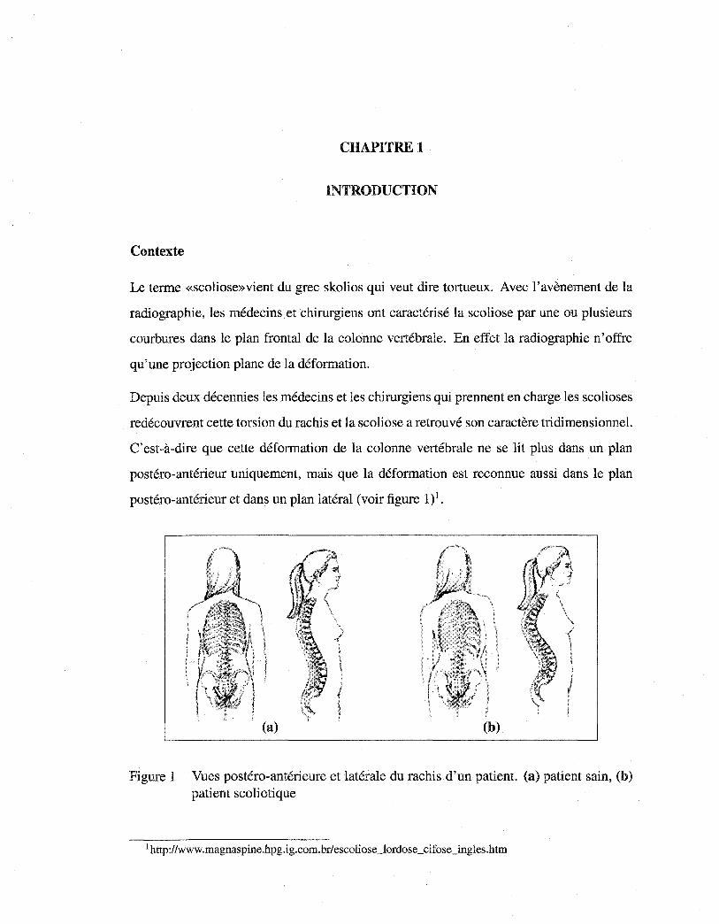
Le terme «scoliose»vient du grec skolios qui veut dire tortueux. Avec l'avènement de la
radiographie, les médecins et chirurgiens ont caractérisé la scoliose par une ou plusieurs
courbures dans le plan frontal de la colonne vertébrale. En effet la radiographie n'offre
qu'une projection plane de la déformation.
Depuis deux décennies les médecins et les chirurgiens qui prennent en charge les scolioses
redécouvrent cette torsion du rachis et la scoliose a retrouvé son caractère tridimensionnel.
C'est-à-dire que cette déformation de la colonne vertébrale ne se lit plus dans un plan
postéro-antérieur uniquement, mais que la déformation est reconnue aussi dans le plan
postéro-antérieur et dans un plan latéral (voir figure 1)1•
(b)
Figure 1 Vues postéro-antérieure et latérale du rachis d'un patient. (a) patient sain, (b) patient scoliotique
1 http://www.magnaspine.hpg.ig.eom.br/escoliose_lordose_cifose_ingles.htm
Reproduced with permission of the copyright owner. Further reproduction prohibited without permission.
2
Les utilisateurs d'imagerie médicale éprouvent un besoin croissant de disposer des infor
mations tridimensionnelles pour améliorer le diagnostic de pathologies complexes comme
la scoliose, afin de mieux évaluer et planifier les méthodes de correction orthopédiques et
chirurgicales. Une représentation de la scoliose en modèle géométrique 3D permet l'accès
à la déformation complète de la colonne tant au niveau global qu'au niveau local, c'est-à
dire pour chacune des vertèbres. De nombreuses méthodes de reconstruction 3D ont été
développées au cours des dernières années pour extraire cette information tridimension
nelle.
Problématique
Les méthodes de reconstruction 3D associées aux systèmes d'imagerie médicale CT
Scan ou IRM permettent d'obtenir des reconstructions tridimensionnelles précises des
structures osseuses humaines. Cependant, le système CT-Scan est très irradiant pour
le patient, un volume important d'information à traiter est nécessaire, et la position al
longée, imposée au patient durant l'examen ne permet pas une étude des déformations
auxquelles le clinicien a habituellement accès, c'est-à-dire sous l'influence de la gravité,
le patient en position debout. Bien que le système IRM est non irradiant, on retrouve les
deux derniers inconvénients du CT-Scan. L'imagerie par ultrasons n'a pas été adaptée à
l'analyse de la forme géométrique tridimensionnelle de la structure osseuse car les struc
tures osseuses génèrent trop d'écho et beaucoup de bruit de mesures (échos parasites à la
forme géométrique des surfaces des structures denses) [26].
L'imagerie médicale par rayons X des structures osseuses est largement utilisée en clin
ique. Dans le cas de la scoliose, l'accès à une information tridimensionnelle personnal
isée, quantitative et fiable est essentiel afin d'assurer un diagnostic amélioré et un traite
ment orthopédique ou chirurgical adéquat. La scoliose nécessite un suivi dans le temps,
pouvant exposer les patients à des quantités importantes de radiation sans vraiment tenir
compte de leur passé radiologique. La scoliose concerne 2 à 4% de la population de
l'Amérique du Nord dont 90% sont des jeunes filles en période de croissance, avec pour
Reproduced with permission of the copyright owner. Further reproduction prohibited without permission.
3
corollaire la nécessité de réduire les doses de radiation administrées à chaque examen con
formément aux nouvelles recommandations internationales pour les examens médicaux
répétitifs. L'utilisation des méthodes de reconstruction 3D multiplanaires pour extraire de
l'information 3D devient donc un impératif de plus haute importance pour les patients, les
chercheurs et la communauté clinique.
Le problème de reconstruction 3D multiplanaire appartient à la classe des problèmes mal
posés au sens de Hadamard. L'acquisition de deux images radiographiques bi planaires ne
fournit qu'un ensemble de données incomplètes qui ne permet pas d'assurer l'unicité de
la solution.
Pour pallier à cette limitation, il est nécessaire de régulariser la procédure de reconstruc
tion 3D en introduisant une connaissance a priori de l'objet à reconstruire. Des modèles
géométriques ont été proposés mais leur grande rigidité ne leur permet pas de prendre en
compte les variabilités anatomiques et celles liées aux pathologies.
Au contraire, les méthodes de reconstruction 3D multiplanaires par modélisation statis
tique, telles que celle que nous proposons dans cette thèse offrent une plus grande soup
lesse de modélisation et permettent de prendre en compte les variabilités anatomiques et
celles liées aux pathologies des structures osseuses à reconstruire.
Objectifs généraux et hypothèses
L'objectif de cette thèse est de développer une méthode de reconstruction 3D de chaque
vertèbre, de la colonne vertébrale et de la cage thoracique scoliotiques à partir de deux
images radiographiques conventionnelles calibrées (postéro-antérieure avec incidence de
oo (IPA) et latérale (hAr)) sous certaines hypothèses2 par modèles statistiques. Dans
le cadre de cette thèse, le problème de reconstruction 3D sera vu comme un problème
d'estimation des paramètres de déformation du modèle ou, de manière équivalente, comme
Reproduced with permission of the copyright owner. Further reproduction prohibited without permission.
4
un problème de minimisation d'une fonction d'énergie. Cette minimisation se fera par un
algorithme d'optimisation déterministe ou stochastique.
Nous supposons qu'il est possible d'obtenir,
- Une modélisation géométrique 3D des vertèbres scoliotiques, précise, et de manière
supervisée en combinant les informations (contours) obtenues des images radio
graphiques !pA et hAT et des informations géométriques a priori de nature statis
tique.
- Une modélisation géométrique 3D de la colonne vertébrale scoliotique, précise, et
de manière non supervisée en combinant les informations (contours) obtenues des
images radiographiques ]pA et hAT et des informations géométriques a priori de
nature statistique.
- Une modélisation géométrique 3D de la cage thoracique scoliotique, précise, et
de manière non supervisée en combinant les informations (contours et régions)
obtenues de 1' image radiographique 1 pA et 1' image hAT comme contrainte et des
informations géométriques a priori de nature statistique.
2Toutes les images radiographiques conventionnelles lpA et hAT utilisées dans la reconstruction 3D de la colonne vertébrale et de la cage thoracique scoliotiques sont issues du système Fuji FCR 7501S disponible à l'hôpital Sainte-Justine de Montréal. L'environnement radiographique est calibré par la technique de calibration utilisée au laboratoire d'informatique de scoliose 3D (LIS-3D) de l'hôpital Sainte-Justine de Montréal. Nous disposons de:
- Une base d'apprentissagede vertèbres (500 normales et 500 scoliotiques) issue de la numérisation de plus de 200 repères anatomiques sur des vertèbres secs par le système Fastrack© dont la précision est 0.2 mm [82].
- Une base d'apprentissage de 532 cages thoraciques scoliotiques issue de la reconstruction 3D stéréoradiographique dont l'erreur moyenne est évaluée à 1.1 mm avec un écart-type de 0.72 mm [24].
- Un échantillon de 57 vertèbres lombaires et thoraciques (13 patients scoliotiques) qui ont été reconstruites par la méthode CT-Scan pour fin de validation.
Reproduced with permission of the copyright owner. Further reproduction prohibited without permission.
5
À cette fin, nous avons construit trois modèles statistiques permettant la reconstruction 3D
de chaque vertèbre, de la colonne vertébrale et de la cage thoracique scoliotiques à partir
de deux images radiographiques conventionnelles calibrées IPA et hAT·
Dans un premier article, nous présentons une méthode statistique supervisée de recon
struction 3D des vertèbres scoliotiques à partir de deux images radiographiques conven
tionnelles calibrées I pA et hAT utilisant les contours de vertèbres détectés sur deux images
radiographiques conventionnelles calibrées et une connaissance géométrique a priori de
nature statistique de chaque vertèbre obtenue par une analyse en composantes principales
appliquée à une base d'apprentissage d'environ 1000 vertèbres (30 vertèbres saines et 30
vertèbres scoliotiques par niveau vertébral). La minimisation de la fonction d'énergie se
fera par un algorithme de descente de gradient [7]. Cette méthode sera validée sur un
échantillon de 57 vertèbres scoliotiques issues de reconstructions CT-Scan.
Dans un second article, nous présentons une méthode statistique non supervisée de recon
struction 3D de la colonne vertébrale scoliotique à partir de deux images radiographiques
conventionnelles calibrées IPA et hAT utilisant les contours de vertèbres détectés sur lpA
et hAT et une connaissance globale hiérarchique a priori de la structure géométrique de
la colonne puis de chaque niveau vertébral. La structure géométrique de chaque niveau
vertébral sera obtenue de la même manière que dans le premier article. La minimisation
de la fonction d'énergie se fera par un algorithme stochastique d'Exploration/Sélection
[33]. Cette méthode sera validée sur un échantillon de 57 vertèbres scoliotiques issues de
reconstructions CT-Scan.
Dans un troisième article, nous présentons une méthode statistique non supervisée de re
construction 3D de la cage thoracique scoliotique à partir de deux images radiographiques
conventionnelles calibrées IPA et hAT utilisant d'une part les contours de la cage tho
racique détectés sur la radiographie IPA et d'autre part une connaissance géométrique a
priori de nature statistique de la cage thoracique obtenue par un mélange d'analyse en
composantes principales probabiliste [92, 93]. Cette connaissance géométrique a pri-
Reproduced with permission of the copyright owner. Further reproduction prohibited without permission.
6
ori est extraite d'une base d'apprentissage de 532 cages thoraciques scoliotiques et les
paramètres de celle ci seront estimés par 1' algorithme Stochastic Expectation Maximiza
tion [33]. La minimisation de la fonction d'énergie se fera par un algorithme stochastique
d'Exploration/Sélection [79]. Cette méthode sera validée sur un échantillon de 20 cages
thoraciques scoliotiques issues de reconstructions stéréo-radiographique [24].
Plan de la thèse
Dans le chapitre 2, nous présentons une revue de littérature pour illustrer la contribution
des travaux précédents à l'élaboration de notre thèse, ainsi que l'originalité de nos princi
pales contributions.
Les trois chapitres suivants correspondent à trois articles. Ils constituent une contribution
originale de 1' auteur de cette thèse au domaine de la vision 3D en imagerie médicale. Nos
idées originales ont été exposées dans des actes de conférences internationales [6] [8] [5].
«3D/2D Registration and Segmentation of Scoliotic Vertebrae Using Statistical Models,
dans Computerized Medical Imaging and Graphies »,publié dans le journal Computerized
Medicallmaging and Graphies, 27(5):321-327, 2003.
«A Hierarchical Statistical Modeling Approach for the Unsupervised 3D Biplanar Recon
struction of the Scoliotic Spine », soumis au journal IEEE Transactions on BioMedical
Engineering, 2004.
«Unsupervised 3D Biplanar Reconstruction of Scoliotic Rib Cage using the Estimation
of a Mixture of Probabilistic Prior Models », soumis au journal IEEE Transactions on
BioMedical Engineering, 2004.
Nous terminons par une discussion générale au chapitre 6, une conclusion et nos recom
mandations au chapitre 7.
Reproduced with permission of the copyright owner. Further reproduction prohibited without permission.
CHAPITRE2
REVUE DE LITTÉRATURE
Nous présentons dans ce chapitre l'état de l'art sur la reconstruction 3D des structures
osseuses antérieures à nos travaux. Ces méthodes sont classées suivant la nature de la
connaissance a priori utilisée pour contraindre le problème mal-posé de reconstruction
3D. Les méthodes présentées sont supervisées et ne disposent pas d'une base d'apprentis
sage de la structure osseuse à reconstruire. Nous nous sommes inspirés de plusieurs idées
générales sous-jacentes à ces méthodes pour développer nos méthodes de reconstruction
3D.
2.1 Méthodes de reconstruction 3D des structures osseuses: état de l'art
À notre connaissance, il n'existe pas dans la littérature de critères de classification de
méthodes multiplanaires de reconstruction 3D. Nous avons distingué trois classes de mé
thodes multiplanaires de reconstruction 3D.
2.1.1 Méthodes de reconstruction 3D sans connaissance a priori
Plusieurs auteurs ont proposé des techniques de reconstruction 3D des vertèbres à partir
de deux vues radiographiques conventionnelles (postéro-antérieure avec incidence de oo (IPA) et latérale (hAr)) [89][83][85][40]. Ces techniques sont basées sur l'identification
de quelques repères anatomiques dans !pA et hAT· Les vertèbres sont alors modélisées
par des quadrilatères 3D.
Dansereau et Stokes ont proposé une méthode de reconstruction 3D de la cage thoracique
à partir de deux vues radiographiques conventionnelles (postéro-antérieure avec incidence
de oo et postéro-antérieure avec incidence de 20° (IPA- 2oo )) [24]. Seules les lignes mé
dianes des côtes sont reconstruites par une méthode itérative combinant 1' algorithme DLT
Reproduced with permission of the copyright owner. Further reproduction prohibited without permission.
8
[71] et des courbes splines. Les points postérieurs des côtes sont déduits d'une recons
truction 3D des vertèbres de la colonne vertébrale. La position du sternum et les points
antérieurs des côtes sont déterminés par des marqueurs radio opaques placés sur la peau.
Ces méthodes sont supervisées et imprécises à cause du fait qu'une erreur d'identification
d'un repère anatomique de 2 mm peut engendrer des erreurs de reconstruction 3D de 5
mm [1]. Martin et Aggarwal ont proposé une méthode de reconstruction 3D à partir des
silhouettes [70] permettant de reconstruire des objets 3D polygonaux par rétroprojection
des silhouettes. Une méthode d'extraction de la géométrie 3D des structures osseuses à
partir de deux vues radiographiques est proposée par Caponetti et Fanelli [14] dans la
quelle le positionnement initial de la structure osseuse 3D issue de la rétroprojection est
ensuite raffiné par une interpolation B-spline.
En raison de la nature du problème mal-posé de reconstruction 3D, une bonne et précise
reconstruction de la structure géométrique 3D ne peut être estimée sans contraintes. Des
méthodes de reconstruction 3D utilisant une connaissance a priori sur la structure géomé
trique de 1' objet à reconstruire ont donc été proposées dans la littérature.
2.1.2 Méthodes de reconstruction 3D avec connaissance géométrique a priori
Pour contraindre le problème inverse mal-posé de reconstruction 3D, il faut introduire une
information sur 1' objet à reconstruire. De nombreuses méthodes ont été proposées dans
la littérature permettant une reconstruction 3D des structures osseuses avec connaissance
géométrique a priori. Terzopoulos et al. ont proposé une méthode permettant de récupérer
la forme 3D des profils d'un objet utilisant comme contrainte géométrique a priori une
combinaison de tubes et colonne vertébrale déformables [90]. La déformation est contrô
lée par des forces physiques internes et externes. Bardinet et al. ont proposé une méthode
permettant de recaler un modèle de superquadriques déformable localement à un ensemble
de points en utilisant des déformations de forme libre [4]. Nik:khade et al. ont présenté une
méthode de reconstruction 3D des fémurs à partir de deux vues radiographiques conven
tionnelles orthogonales [78]. Cette méthode consiste à recaler des surfaces paramétriques
Reproduced with permission of the copyright owner. Further reproduction prohibited without permission.
9
cubiques aux trois parties du fémur puis à les rassembler en un seul modèle complet. Kita
a présenté un modèle déformable 3D permettant d'analyser les images radiographiques
de l'estomac [57]. Le modèle a priori est un tube dont l'initialisation est réalisée avec
une seule image radiographique. Le modèle est ensuite déformé en utilisant les autres
images. Une méthode multiplanaire de reconstruction 3D à partir de deux vues radiogra
phiques conventionnelles est présentée par Dansereau et Stokes [24]. Elle est basée sur
la numérisation de six repères anatomiques stéréo-correspondants par vertèbre (centroïdes
des plateaux vertébraux, sommets des pédicules) sur les deux images radiographiques. Ces
repères anatomiques seront ensuite reconstruits en 3D par l'algorithme DLT [71]. Un mo
dèle surfacique est ensuite déformé par krigeage dual [94] pour s'ajuster aux repères anato
miques reconstruits. Mitton et al. ont amélioré cette méthode en tenant compte des repères
anatomiques stéréo-correspondants et non stéréo-correspondants [75]. Les points du mo
dèle de vertèbre reconstruit, reliés entre eux par des ressorts linéaires, sont contraints à se
déplacer le long des lignes épipolaires. Le modèle est ensuite déformé vers un état méca
nique stable. Ces deux méthodes sont tout d'abord supervisées, imprécises et n'exploitent
pas toute l'information contenue dans les deux images radiographiques (par exemple, les
contours de chaque vertèbre). Huynh et al. ont modélisé la cunéiformisation vertébrale1
par des modèles d'ellipses [52]. Cette modélisation est basée sur la numérisation d'une
suite de points sur les contours des plateaux vertébraux sur les deux images radiogra
phiques. Les points stéréo-correspondants de cette suite sont reconstruits par l'algorithme
DLT [71]. Le contour reconstruit des plateaux vertébraux est modélisé par une ellipse dont
la forme et la position sont optimisées par un processus itératif. Pour réaliser la mise en
correspondance des courbes sur les deux images radiographiques, un ensemble de points
est généré mathématiquement sur 1' ellipse, puis réprojetés sur les deux images. Ces points
sont alors déplacés pour se superposer sur les points correspondants des contours déjà mo-
1Disparition de l'aspect parallèle des plateaux vertébraux d'une ou plusieurs vertèbres sur une projection frontale ou sagittale.
Reproduced with permission of the copyright owner. Further reproduction prohibited without permission.
10
délisés par des courbes splines. Delorme et al. ont adopté cette technique de modélisation
de la cunéiformisation vertébrale par des modèles d'ellipses dans [27].
Lotjonen et al. ont proposé une méthode de reconstruction 3D d'un thorax à partir de
deux vues radiographiques conventionnelles [64]. Cette méthode consiste à simuler les
images radiographiques du modèle, et de construire ensuite les champs des déformations
élastiques 3D nécessaires pour recaler les images simulées avec les images réelles. Veistera
et al. ont appliqué cette méthode à la reconstruction 3D du coeur [95].
Toutes ces méthodes soulèvent deux problèmes. D'une part, elles proposent des modèles
géométriques dont la rigidité ne leur permet pas de prendre en compte les variabilités
anatomiques et les pathologies (cas de la scoliose). D'autre part, elles n'exploitent pas la
connaissance statistique des déformations possibles de 1' objet à reconstruire. Par consé
quent, la forme 3D reconstruite ne correspond pas nécessairement à la réalité. Ces incon
vénients peuvent être surmontés par une approche statistique.
2.1.3 Méthodes de reconstruction 3D avec connaissance statistique a priori
L'approche statistique permet la prise en compte des connaissances a priori sur la struc
ture des objets et leurs déformations, ce qui introduit une robustesse appréciable dans les
techniques de recalage ou de reconstruction 3D.
Les deux approches que nous présentons dans cette thèse s'inspirent de travaux qu'il nous
a semblé nécessaire de décrire. La première approche (approche modale), qui a été présen
tée à l'origine par Cootes et al. [20][22], est adaptée spécifiquement pour notre problème
de reconstruction 3D des vertèbres et de la colonne vertébrale scoliotiques. La seconde ap
proche (approche de mélange de modèles de forme a priori), qui a été présentée à l'origine
par Tipping et Bishop [92][93], est retenue pour la reconstruction 3D de la cage thoracique
scoliotique.
Reproduced with permission of the copyright owner. Further reproduction prohibited without permission.
11
2.1.3.1 Travaux de Cootes
Les modèles statistiques linéaires ont été popularisé par les travaux de Cootes [22] [20] et
ont permis la création et l'utilisation de modèles de formes et d'apparence en 2D, après
apprentissage supervisé. Au sein de ces modèles, la variabilité est prise en considération
dans un cadre linéaire et modélise ainsi les déformations statistiquement admissibles par
le modèle.
Ce modèle a essentiellement été utilisé en segmentation d'images fixes et pour le suivi tem
porel d'images d'organes humains. Kervrann et Heitz [55] ont proposé quelques amélio
rations à ce modèle. Tout d'abord, les déformations sont estimées dans un cadre bayésien.
Ensuite, une description hiérarchique permet de distinguer nettement les déformations glo
bales des modes de déformations obtenus dans la base d'apprentissage. L'estimation des
paramètres qui décrivent la forme globale de l'objet d'intérêt est effectuée préliminaire
ment à l'estimation des déplacements locaux.
De nombreux auteurs [37] [47] ont adapté les modèles statistiques linéaires de Cootes aux
problèmes 3D. En imagerie médicale, la modélisation des déformations permet la carac
térisation et l'interprétation des pathologies des structures osseuses. Fleute et Lavallée ont
proposé une méthode de reconstruction 3D à partir de multi acquisitions radiologiques
calibrées basée sur l'identification des contours dans les images radiographiques [39]. Un
modèle statistique est créé à partir de plusieurs modèles surfaciques obtenus par recons
truction CT-Scan supervisée et une analyse en composante principale (ACP ou transformé
de Karhunen-Loeve) sur cet ensemble de géométries. La reconstruction 3D est obtenue par
déformation du modèle statistique de sorte que les contours projetés du modèle reconstruit
s'adaptent au mieux aux contours identifiés dans les radiographies. Lorenz et Krahnstü
ver ont proposé un modèle 3D de vertèbre lombaire à partir d'un ensemble de vertèbres
représentatives préalablement numérisées par tomographie [62]. Mouren a proposé dans
[77] une méthode de reconstruction 3D de la cage thoracique scoliotique à partir de lpA
et hAr, semblable à celle proposé précédemment dans nos travaux [7] pour la reconstruc-
Reproduced with permission of the copyright owner. Further reproduction prohibited without permission.
12
tion de vertèbres scoliotiques. Cette méthode consiste à reconstruire la cage thoracique
côte par côte. La reconstruction de côte consiste à déformer un modèle de forme sta
tistique de côte afin de recaler les projections (postéro-antérieure et latérale) du contour
externe de ce modèle a priori 3D de côte avec les contours de la côte correspondante
préalablement segmentés sur les deux vues radiographiques !PA et hAT· Le positionne
ment initial du modèle déformable de chaque côte est réalisé par l'utilisation de quelques
points numérisés manuellement dans la vue radiographique hAT· Cette méthode est su
pervisée et l' ACP n'est pas toujours la bonne solution pour la caractérisation des modes
de déformation d'une structure osseuse (cf. Chap. 4).
2.1.3.2 Travaux de Tipping et Bishop
L'approche de mélange de modèles a priori2 pourrait être qualifiée d'approche "linéaire
par morceaux". Elle a été proposée initialement par Tipping et Bishop [92][93]. Cette
approche considère le modèle global non linéaire comme un mélange de modèles locale
ment linéaires qui fournissent des "clusters" ou "classes" de formes. Chacun de ces sous
modèles peut alors être analysé par une analyse en composantes principales probabiliste
qui fournit une réduction de dimension pour chacun d'entre eux. Les paramètres de ces
sous-modèles sont estimés par des algorithmes de type EM (Expectation Maximisation)
au sens du ML (Maximum Likelihood).
Dans ce type d'approches, se pose notamment la question du choix du nombre de compo
santes du mélange, à laquelle il n'est pas forcément évident de répondre, ainsi que celle
du choix du nombre de composantes principales à retenir pour la définition de l'espace
de travail de dimension réduite. En plus, l'algorithme itératif EM est sensible à l'initiali
sation, il converge extrêmement lentement et la convergence vers un bon maximum n'est
pas assurée.
2Cette approche est connue sous le nom de mélange d'analyses en composantes principales probabilistes.

Reproduced with permission of the copyright owner. Further reproduction prohibited without permission.
13
Mentionnons que l'analyse en composantes principales probabiliste a été déjà utilisée dans
la localisation de forme dans une image [32], la classification d'objets [35] et l'inférence
3D de la structure [41]. Il a été seulement exploité dans la compression d'images [92] mais,
à notre connaissance, il n'a pas été utilisé pour la modélisation 3D en imagerie médicale.
Reproduced with permission of the copyright owner. Further reproduction prohibited without permission.
14
RECALAGE 3D/2D ET SEGMENTATION DES VERTÈBRES SCOLIOTIQUES PAR MODÈLES STATISTIQUES
Article : 3D/2D Registration and Segmentation of Scoliotic Vertebrae Using Statisti
cal Models
Cet article a été publié comme l'indique la référence bibliographique
S. Benarneur, M. Mignotte, S. Parent, H. Labelle, W. Skalli, J. De Guise. 3D/2D registra
tian and segmentation of scoliotic vertebrae using statistical models. Computerized Medi
callmaging and Graphies, 27(5) :321-327, Septembre 2003.
Cet article est présenté ici dans sa version originale.
Résumé
La scoliose est une déformation tridimensionnelle de la courbe naturelle de la colonne
vertébrale, incluant des rotations et des déformations vertébrales. Afin d'étudier et d'ana
lyser des caractéristiques 3D de cette déformation, différentes méthodes de reconstruction
3D de la colonne vertébrale scoliotique à partir d'images multiplanaires ont été dévelop
pées. Ces caractéristiques servent pour la conception, l'évaluation et l'amélioration des
méthodes de correction orthopédiques ou chirurgicales de la colonne vertébrale scolio
tiques. La majorité des méthodes existantes dans la littérature utilisent un nombre restreint
de repères anatomiques numérisés sur les images radiographiques et n'exploitent pas tout
le potentiel d'information (notamment les contours) dans les deux images radiographiques
[75] [43] [76].
Nous présentons dans cet article une méthode statistique supervisée de reconstruction
3D des vertèbres scoliotiques à partir de deux images radiographiques conventionnelles
(postéro-antérieure avec incidence de oo et latérale) calibrées. Cette méthode est basée
sur une connaissance a priori globale de la structure géométrique de la vertèbre. Cette
Reproduced with permission of the copyright owner. Further reproduction prohibited without permission.
15
connaissance est issue d'une base d'apprentissage d'environ 1000 vertèbres (30 vertèbres
saines et 30 vertèbres scoliotiques par niveau vertébral) et représentée par un modèle défor
mable statistique intégrant, en plus des déformations linéaires, une série de déformations
non linéaires modélisées par les premier modes de variation des déformations de l'expan
sion de Karhunen-Loeve. Cette première étape nous permettra d'établir un modèle a priori
paramétrique concis de forme tridimensionnelle qui sera ensuite utilisé pour contraindre
notre problème de reconstruction 3D. Le positionnement initial du modèle déformable
statistique dans l'espace radiographique est réalisé à l'aide de six repères anatomiques
(centroïdes des plateaux vertébraux, sommets des pédicules). La méthode de reconstruc
tion présentée consistera alors à ajuster les projections (postéro-antérieure et latérale) de
ce modèle 3D de la vertèbre avec les contours préalablement segmentés de la vertèbre cor
respondante sur les deux images radiographiques. Le problème de reconstruction 3D est
vu comme un problème d'estimation des paramètres de déformation de ce modèle ou, de
façon équivalente, comme un problème de minimisation d'une fonction d'énergie. Cette
minimisation est réalisée par une technique de descente de gradient simplifiée. La méthode
présentée est validée sur une base de 57 vertèbres lombaires et thoraciques de 13 patients
scoliotiques qui ont aussi été reconstruites par CT-scan pour des fins de comparaison. Une
erreur moyenne de (0. 71 ± 0.06) mm pour les vertèbres lombaires et de (1.48 ± 0.27) mm
pour les vertèbres thoraciques est obtenue sur les distances point-surface entre le modèle
reconstruit avec notre méthode et le modèle issu de la reconstruction CT-scan.
Reproduced with permission of the copyright owner. Further reproduction prohibited without permission.
CHAPITRE3
3D/2D REGISTRATION AND SEGMENTATION OF SCOLIOTIC VERTEBRAE USING STATISTICAL MODELS
Abstract
We propose a new 3D/2D registration method for vertebrae of the scoliotic spine, using
two conventional radiographie views (postero-anterior and lateral), and a priori global
knowledge of the geometrie structure of each vertebra. This geometrie knowledge is effi
ciently captured by a statistical deformable template integrating a set of admissible defor
mations, expressed by the first modes of variation in Karhunen-Loeve expansion, of the
pathological deformations observed on a representative scoliotic vertebra population. The
proposed registration method consists of fitting the projections of this deformable tem
plate with the preliminary segmented contours of the corresponding vertebra on the two
radiographie views. The 3D/2D registration problem is stated as the minimization of a cost
function for each vertebra and solved with a gradient descent technique. Registration of the
spine is then done vertebra by vertebra. The proposed method efficient! y provides accurate
3D reconstruction of each scoliotic vertebra and, consequently, it also provides accurate
knowledge of the 3D structure of the whole scoliotic spine. This registration method has
been successfully tested on several biplanar radiographie images and validated on 57 scol
iotic vertebrae. The validation results reported in this paper demonstrate that the proposed
statistical scheme performs better than other conventional 3D reconstruction methods.
Key words: 3D/2D registration, 3D reconstruction model, statistical deformable model,
shape model, biplanar radiographies, scoliosis, medical imaging, energy function opti
mization.
Reproduced with permission of the copyright owner. Further reproduction prohibited without permission.
17
3.1 Introduction
Registration, an important problem in computer vision, is still incompletely solved. It
primarily consists of establishing a geometrie relation between the objects represented by
two images. Many methods of image registration have been proposed in the literature (see,
for example, a good survey of image registration methods proposed by Brown in [12], and
the excellent review of existing registration techniques proposed by Van den Eisen et al in
[30], Lavallée in [59], or Maintz and Viergever in [67], specifie to the medical image reg
istration problem). A comparison between several registration approaches has been also
undertaken by West in [97]. Registration is a problem common to many tasks in medical
imagery. Among these tasks, we can cite the 3D reconstruction of anatomical structures,
the fusion of information coming from severa! methods, the construction of anatomical
and functional atlases in medical imaging (allowing the detection of local and/or anatom
ical or functional abnormalities), the voluminal and dynamic visualization of images, etc.
In our application, we use a 3D/2D statistical registration model from biplanar radio
graphie images for the 3D reconstruction of scoliotic vertebrae of a spine. Scoliosis is a
3D deformation of the natural curve of the spinal column, including rotations and verte
bral deformations. To analyze the 3D characteristics of these deformations, which can be
useful for the design, evaluation and improvement of orthopedie or surgical correction,
several 3D reconstruction methods have been developed. The 3D reconstruction methods
oftomodensitometric imagery modalities (e.g., X-rays, magnetic resonance) provide accu
rate 3D information of the human anatomy. However, the high level of radiation received
by the patient, the large quantity of information to be acquired and processed, and the
cost of these methods make them less functional [43]. 3D reconstruction methods using
a limited number of projections and sorne simple a priori knowledge of the geometry of
the object to be reconstructed are interesting but are widely supervised; for example they
may require manual identification (by an operator) of a set of 19 different points of interest
(landmarks) on two different radiographie images (postero-anterior with normal incidence
Reproduced with permission of the copyright owner. Further reproduction prohibited without permission.
18
(!PA) and lateral (hAT)) of 17lumbar and thoracic vertebrae [43][75][76]. Besides, these
afore-mentioned methods may not be very accurate, especially because they do not exploit
aU the information contained in the two radiographie images (e.g., the contours of each
vertebra or a priori global geometrical knowledge of the object to be reconstructed), and
because they are highly operator-dependent. To this end, Bayesian inference or statisti
cal modeling is a convenient way of taking a priori information into consideration. The
statistical approach is quite popular and has been successfully applied in medical imagery
[21][19][68], in image analysis for extracting 2D objects in an image [22] or in an image
sequence [56], for the 3D representation of vertebra [62], nonrigid 3D/2D registration of
theknee [39][38], segmentationof2D anatomical structures [23][49][46][48], localization
and classification [36], etc.
In this way, we propose a new 3D/2D registration modeling approach for scoliotic ver
tebrae from biplanar radiographie images which can be viewed as a new statistical 3D
reconstruction method. Our approach relies on the description of each vertebra by a de
formable 3D template which incorporates (statistical) knowledge about its geometrical
structure and its pathological variability. The deformations of this template are expressed
by the first modes of variation in Karhunen-Loeve (KL) expansion of the pathological
deformations observed on a representative scoliotic vertebra population. This prototype
template, along with the set of admissible deformations, constitutes our global a priori
model that will be used to rightly constraint the ill-posed nature of our 3D/2D registration
problem [44]. In our application, the proposed method consists of fitting this template
with the segmented contours of the corresponding vertebra on two calibrated radiographie
views. This matching problem leads to an optimization problem of a cost function, effi
ciently solved in our application by a gradient descent algorithm initialized by a rough and
rigid 3D/2D registration method estimated in the least square sense.
This paper is organized as follows. Section 3.2 presents the statistical deformable model.
Section 3.3 describes the proposed 3D/2D registration method. Section 3.4 discusses the
Reproduced with permission of the copyright owner. Further reproduction prohibited without permission.
19
validation protocol of our method. The experimental results of our 3D/2D registration or
3D reconstruction method are presented in Section 3.5. Finally, we conclude the paper in
Section 3.6 with a discussion and perspectives.
3.2 Statistical Deformable Model
The shape s of each vertebra is defined by a set of l control points or landmarks, which
approximate the geometrie shape of each vertebrain R} [22]. Bach vertebra, in the training
set, is thus represented by the following 3l dimensional vector,
where (xi, Yi, zi)t are the Cartesian coordinates of each surface point. In the following, we
will assume that s is the realization of a random vector that follows a normal law of mean
vector sand covariance matrix C, as suggested in [22]. After alignment of the N training
shapes [22], the mean shape and the covariance matrix are defined as,
1 N s=- L::si,
N i=l
The variabilities within the training set are characterized by the displacement vector s =
s - s of the different surface points with respect to the mean model. Statistical analysis
of this random vector makes it possible to deduce the deformation modes relative to the
mean shape. The eigenvectors of the covariance matrix C of this random vector describe
the variation modes in the deformation parameter space or information on the variability
of scoliotic deformations in the vertebra database. The associated eigenvalues Ài are the
amplitudes of these variation modes. An accurate description of the main variation modes
may be obtained by retaining only them eigenvectors associated with the t largest eigen-
Reproduced with permission of the copyright owner. Further reproduction prohibited without permission.
20
values1• [22]. The model allows the generation of new instance of the shape by adding
linear combinations of the m most significant variation vectors to the mean shape,
s = <I> b + s, (3.1)
where <I> represents an orthogonal base of variation modes of scoliotic vertebrae contained
in the training base, and bis the global deformation parameter vector setting the amplitudes
of each deformation mode bi. By ensuring,
(3.2)
where Ài is the eigenvalue associated with the deformation mode bi, only the important
deformations are extracted, discarding training data noise [22]. This low parametric rep
resentation of a vertebra constitutes to our global a priori model that will be used in our
3D reconstruction method (cf. Figures 2 and 3).
In theory, the ratio of an eigenvalue to the total sum of the other eigenvalues expresses
the percentage of error introduced if the eigenvector associated with the corresponding
eigenvalue is not selected [22]. One must thus specify a threshold !v Uv E [0, 1]) for the
eigenvalues above which the error is considered to be sufficiently small to generate a good
approximation of the initial vector. Hence, if Vr is the sum of the eigenvalues, then the
number m of eigenvalues to be selected is such that,
m
2::: Ài ~ fv Vr, (3.3) i=l
1 As C is symmetric (cr = C), its eigenvalues are real and the associated eigenvectors are orthogonal. As C is positive definite, its eigenvalues are positive or null.
Reproduced with permission of the copyright owner. Further reproduction prohibited without permission.
21
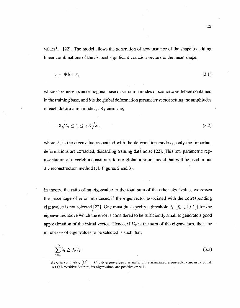
Figure 2 Visualization of mean shape (middle row) from the sagittal (top row) and coronal views (bottom row), and two deformed shapes obtained by applying (±3 standard deviations of the first and second deformation modes to the mean shape for the L3 vertebra
By doing so, we ensure that the selected deformation modes allow us to represent lOOfv%
of the existing scoliotic deformations in the training base2 .
2Each vector can also be characterized by the Mahalanobis distance ( s - s) T c-l ( s - s) directly related to a normal distribution. From relation 3.2, we deduce that [22],
m b2 L Ài· ::.:; 9m. (3.4) i=l '
A random vector s which does not check this condition could be considered to be not representative with respect to statistical training. In practice, the criterion expressed by Eq. 3.4 could be used to validate certain configurations of shapes [23].
Reproduced with permission of the copyright owner. Further reproduction prohibited without permission.
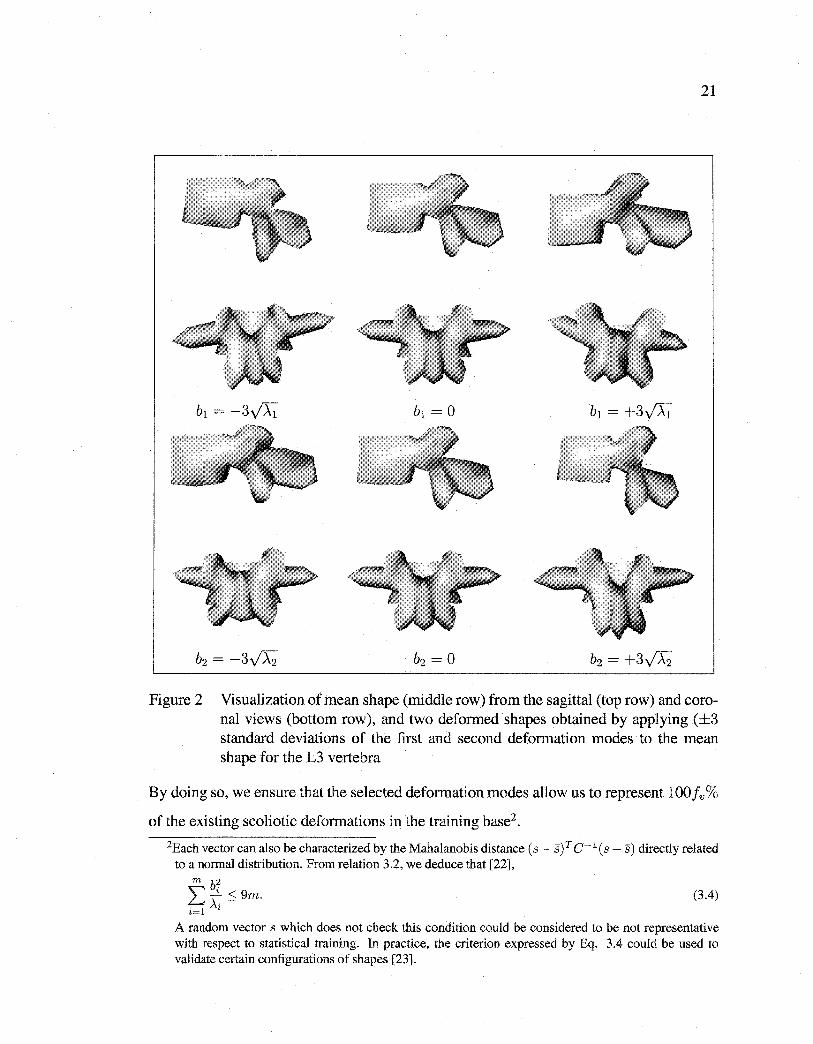
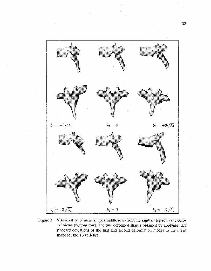
22
Figure 3 Visualization of mean shape (middle row) from the sagittal (top row) and coronal views (bottom row), and two deformed shapes obtained by applying (±3 standard deviations of the first and second deformation modes to the mean shape for the T6 vertebra
Reproduced with permission of the copyright owner. Further reproduction prohibited without permission.
23
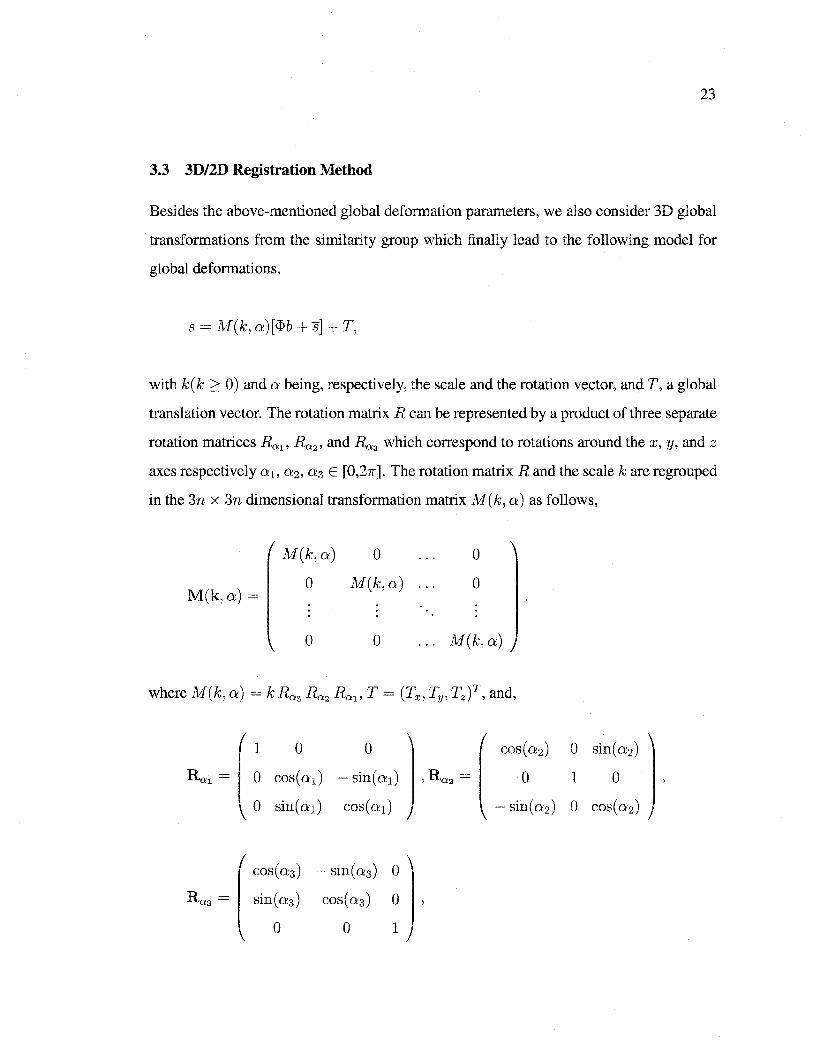
3.3 3D/2D Registration Method
Besides the above-mentioned global deformation parameters, we also consider 3D global
transformations from the similarity group which finally lead to the following model for
global deformations,
s = M(k, a)[<J?b + s] + T,
with k(k 2: 0) and a being, respectively, the scale and the rotation vector, and T, a global
translation vector. The rotation matrix R can be represented by a product of three separate
rotation matrices Rap Ra2 , and Ra3 which correspond to rotations around the x, y, and z
axes respectively a:1, a:2 , a:3 E [0,27r ]. The rotation matrix Rand the scale k are regrouped
in the 3n x 3n dimensional transformation matrix M(k, a) as follows,
M(k, a) 0
M(k, a:)= 0 M(k, a)
0 0
1 0 0
0 cos(a:1 ) -sin(a:1 )
0 sin(a:1) cos(a:1)
cos( a:3) -sin( a:3) 0
Ras = sin(a:3) cos(a:3) 0
0 0 1
0
0
M(k,a)
Reproduced with permission of the copyright owner. Further reproduction prohibited without permission.
24
3.3.1 Crude and Rigid Initial Registration
To ensure a first erode and rigid reconstruction of each vertebra, we use the technique
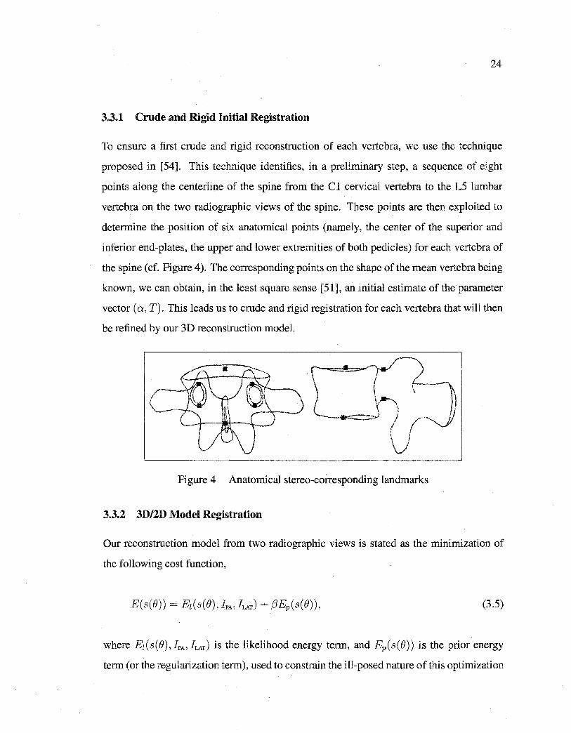
proposed in [54]. This technique identifies, in a preliminary step, a sequence of eight
points along the centerline of the spine from the Cl cervical vertebra to the L5 lumbar
vertebra on the two radiographie views of the spine. These points are then exploited to
determine the position of six anatomical points (namely, the center of the superior and
inferior end-plates, the upper and lower extremities of both pedicles) for each vertebra of
the spine (cf. Figure 4 ). The corresponding points on the shape of the mean vertebra being
known, we can obtain, in the least square sense [51], an initial estimate of the parameter
vector (a, T). This leads us to erode and rigid registration for each vertebra that will then
be refined by our 3D reconstruction model.
Figure 4 Anatomical stereo-corresponding landmarks
3.3.2 3D/2D Model Registration
Our reconstruction model from two radiographie views is stated as the minimization of
the following cost function,
(3.5)
where Ez(s(B), IPA' JLAT) is the likelihood energy term, and Ep(s(B)) is the prior energy
term (or the regularization term), used to cons train the ill-posed nature of this optimization
Reproduced with permission of the copyright owner. Further reproduction prohibited without permission.
25
problem. (3 is a factor that provides relative weighting between the two penalty terms and
allows us to control the rigidity of the statistical template [53]. () = (M(k, a), T, b) is the
deformation parameter vector of the model to be estimated. It should be noted that this
optimization problem can also be formulated as the search for the maximum a posteriori
(MAP) of(), the deformation parameters of the deformed template s,
()* = argmaxP(lpA, hAT 1 s(O))P(s(e)), ()
(3.6)
where P(IpA, hAT 1 s(e)) = t exp ( -Ez(s(B), !PA' !LAT)) is the likelihood of the obser
vations (i.e., the segmented contours on the two radiographie views) given by a deformed
template, and P ( s ( B)) = (~ exp (-Ep ( s ( ()))) is the prior probability of the deformed tem
plate (or the prior probability of a scoliotic deformation for a given vertebra). (z and (p are
two constants of normalization.
3.3.3 Likelihood Energy Term
In our application, our likelihood model is expressed by a measure of similarity between
the extemal contour of the lateral and the postero-anterior perspective projections of the
deformed template and an edge potential field estimated on the two radiographie views.
First, this edge potential field requires the preliminary detection of edges in the two ra
diographie images. To do so, we use a Canny edge detector [13]. Second, this field is
determined by the positions of the detected edges in the radiographie images. For a pixel
(x, y) in the postero-anterior or lateral image, we define its edge potential by,
Reproduced with permission of the copyright owner. Further reproduction prohibited without permission.
26
where ( Çx, f;,y) is the displacement to the nearest edge point in the image, and T is a smooth
ing factor which controls the degree of smoothness of this potential field3 . This edge
potential induces an energy function that relates a deformed template s to the edges in the
two radiographie images I pA and hAT (cf. Figure 11)
(3.7)
where the summation of the first and second term of Ez(s(B), IPA' !LAT) is overall the nPA
and nLAr points of the extemal contour of the, respectively, lateral and postero-anterior
perspective projections of the deformed template on the two pre-computed edge poten
tial fields of each radiographie image. This energy function attains its maximum value
when there is an exact correspondence between the projected contours (of the deformed
template) and the preliminary segmented contours of the two radiographie views.
3.3.4 Prior Energy Term
Due to Karhunen-Loeve transformation, the random variables bi are independent and fol
low a normal law of a null mean and variance .\i [22]. Thus, the law ofprobability of s(B),
the deformed template, can be written as [56],
m 1 ( b2) P(s(B)) =II ~exp - 2~. ,
i=l t1f t
3We can easily complete this edge potential field IJ!(x, y) by adding to it a directional component to obtain a directional edge potential field,
IJ!'(x,y) = IJ!(x,y) 1 cos('-y(x,y)) !,
where ')'(x, y) is the angle between the tangent of the nearest edge and the tangent direction of the contour at (x, y). This potential field is similar to the one proposed in [53] for a template-based localization approach.
Reproduced with permission of the copyright owner. Further reproduction prohibited without permission.
27
This probability expresses the fact that the shape to be reconstructed is likely close to the
mean shape. By considering that P( s( 8)) = fp exp (-Ep( s( 8))) the prior energy term can
be written as,
(3.8)
This energy term penalizes the deviation of the deformed template from the mean shape.
This term does not penalize affine transformations. Bq. 3.8 closely resembles the Maha
lanobis distance. It defines an ellipsoid centered in Rm whose principal axes are identified
by A when Ep(s(B)) is a constant.
3.3.5 Silhouette Extraction of the 3D Model
The 3D model of vertebrae is represented in the form of a triangulated mesh (cf. Figure
6). Silhouette detection is based on estimation of the normal at each vertex of the mesh.
The normal in each vertex is computed by the average of the normal of ali facets to which
the vertex belongs (cf. Figure 7). For two neighbours 1li and V2 of facet Fi whose product
of the weights is negative, we interpolate linearly along the edge (1/i, V2) (cf. Table 1).
The line joining two interpolated vertices of Fi is called the extemal edge (cf. Figure
8). On a surface r, the extemal edges of the vertebra shape are lines where the direction
of projection is tangent on the surface [16][86]. The extemal edges are saved in a list.
As in the case of a not-convex object, the extemal edges can be hidden by other parts of
the surface. We keep ali the extemal edges, including those that are occluded (i.e., those
that are hidden by another part of the vertebra). Let us recall that we use semi-transparent
radiographie images (i.e., superposition of the various structures on the same plane). In our
application, occluded edges are also exploited in our 3D/2D registration method. Let us
put all the extemal edges having a joint vertex in a list. Bach one of these lists constitutes
an extemal contour of the vertebra. The set of these extemal contours constitutes the
silhouette of the vertebra (cf. Figure 9). We summarize the whole procedure in Table 1.
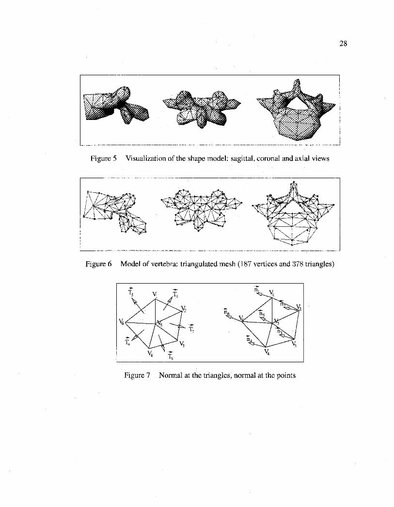
Reproduced with permission of the copyright owner. Further reproduction prohibited without permission.
28
Figure 5 Visualization of the shape model: sagittal, coronal and axial views
Figure 6 Model of vertebra: triangulated mesh (187 vertices and 378 triangles)
Figure 7 Normal at the triangles, normal at the points
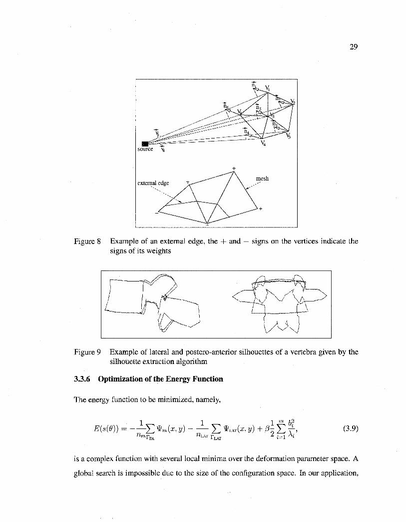
Reproduced with permission of the copyright owner. Further reproduction prohibited without permission.
29
+
mesh extefi!al edge
+
Figure 8 Example of an extemal edge, the + and - signs on the vertices indicate the signs of its weights
Figure 9 Example of lateral and postero-anterior silhouettes of a vertebra given by the silhouette extraction algorithm
3.3.6 Optimization of the Energy Function
The energy function to be minimized, namely,
(3.9)
is a complex function with severallocal minima over the deformation parameter space. A
global search is impossible due to the size of the configuration space. In our application,
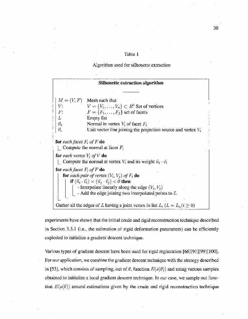
Reproduced with permission of the copyright owner. Further reproduction prohibited without permission.
Table 1
Algorithm used for silhouette extraction
Silhouette extraction algorithm
M = (V,F) V:
Mesh such that V= {VJ., ... , Vn} C R3 Set ofvertices
F: F = { F1 , ... , Ft} set of facets L Empty list
Normal in vertex Vi of facet Fi Unit vector line joining the projection source and vertex Vi
for each facet Fi ofF do L Compute the normal at facet Fi
for each vertex Vi ofV do L Compute the normal at vertex Vi and its weight ni . vi
for each facet Fi ofF do for each pair of vertex (Vi, Vj) of Fi do
l if (ni· vi) x (nj · vj) < o then
l -Interpolate linearly along the edge (Vi, Vj) - Add the edge joining two interpolated points to L
Gather all the edges of L having a joint vertex in list Li (L = Li/i 2: 0)
30
experiments have shown that the initial erode and rigid reconstruction technique described
in Section 3.3.1 (i.e., the estimation of rigid deformation parameters) can be efficiently
exploited to initialize a gradient descent technique.
Various types of gradient descent have been used for rigid registration [66][91][99][100].
For our application, we combine the gradient descent technique with the strategy described
in [53], which consists of sampling, out of(), function E(s(O)) and using various samples
obtained to initialize a local gradient descent technique. In our case, we sample out func
tion E( s( 0)) around estimations given by the erode and rigid reconstruction technique
Reproduced with permission of the copyright owner. Further reproduction prohibited without permission.
31
presented in Section 3.3.1. The final adopted solution is the one associated with the lowest
energy. However, the sampling of these template positions and transformation parameters
must be chosen judiciously. It should be fine enough not to miss the significant local min
ima of the energy function, and large enough to avoid high computational requirements.
In our application, we also use a simplified version of the traditional gradient descent tech
nique, which does not require an analytical expression of the gradient of E( s( fJ)) (clearly
unavailable in our case), and similar to the one proposed in [73]. We have summarized the
whole procedure in Table 2. This gradient descent technique, combined with the above
mentioned sampling strategy, is deployed to simultaneously refine the estimation of rigid
parameters and to estimate nonrigid parameters.
3.4 Validation of 3D/2D Registration
In our application, our 3D/2D registration technique is validated by comparing the recon
structed model obtained by our method and by reconstruction from CT-scan slices [34] by
Sliceümatic© (Tomo Vision. http://www.tomovision.com/) software. 3D reconstruction
models of the vertebrae contain up to 7, 000 points per vertebra and will constitute the
ground truth for our validation procedure. First, the validation procedure consists of fit
ting the model of 200 points of our 3D/2D registration method on the scanned vertebra. To
this end, we manually extract sorne easily identifiable anatomicallandmarks on the recon
structed model resulting from CT-scan whose position is known, and we estimate the rigid
transformation allowing us to pass from the set of anatomical landmarks of our recon
structed model to the set of corresponding anatomical landmarks on the scanned model.
Then, we apply this rigid transformation to all points of the reconstructed vertebra. Once
this is done, we optimize the rigid transformation, which enables us to readjust the two
models of vertebra. Optimization consists of finding neighbours on the scanned vertebra
to each point of the reconstructed vertebra and then of estimating and re-applying the rigid
deformation, allowing us to pass from the set of points of the reconstructed vertebra to the
set of points closes to the scanned vertebra.
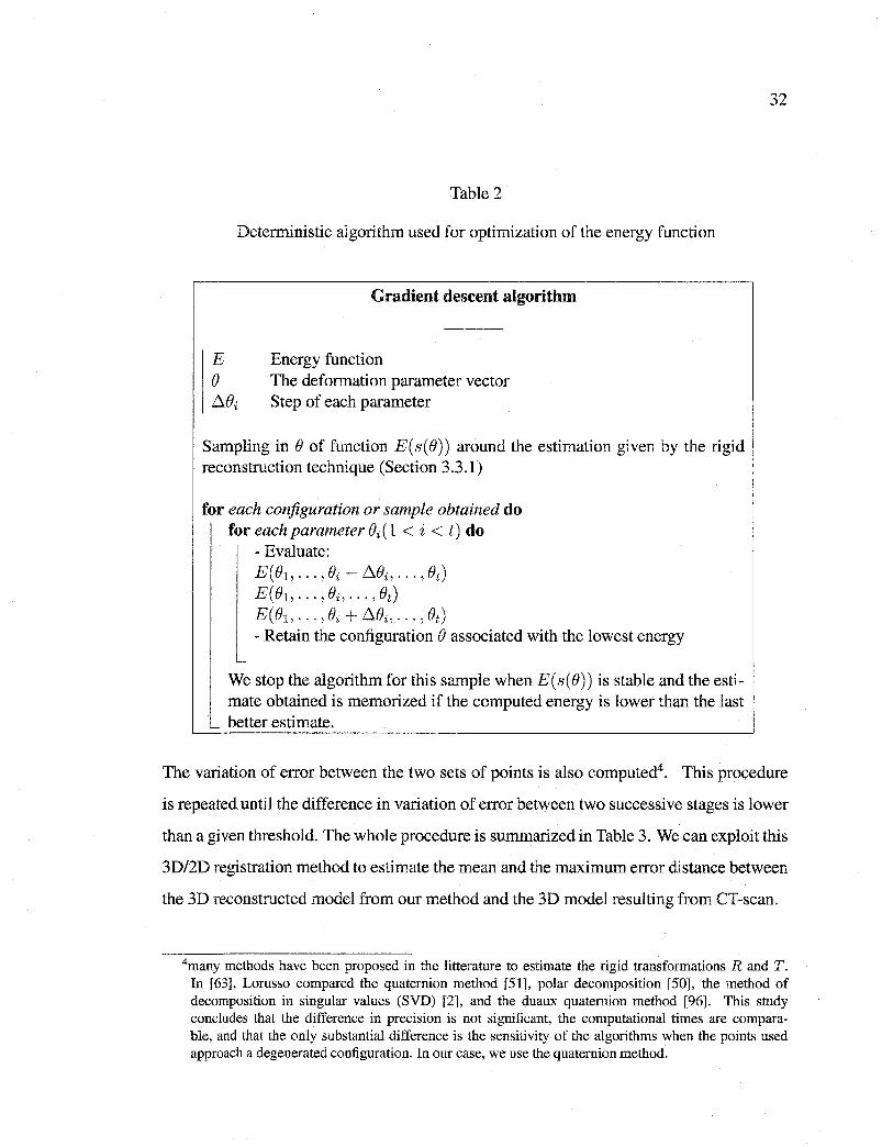
Reproduced with permission of the copyright owner. Further reproduction prohibited without permission.
Table 2
Deterministic algorithm used for optimization of the energy function
Gradient descent algorithm
E Energy function () The deformation parameter vector f:l.()i Step of each parameter
Sampling in() of function E(s(B)) around the estimation given by the rigid reconstruction technique (Section 3.3.1)
for each configuration or sample obtained do for each parameter Bi(l < i < t) do
- Evaluate: E(B1, ... , Bi -l:l.Bi, ... , Bt) E(B1, ... , Bi, ... , Bt) E(B1, ... , ()i + f:l.()i, ... , Ot) - Retain the configuration () associated with the lowest energy
-
We stop the algorithm for this sample when E( s( e)) is stable and the estimate obtained is memorized if the computed energy is lower than the last
_ better estimate.
32
The variation of error between the two sets of points is also computed4• This procedure
is repeated until the difference in variation of error between two successive stages is lower
than a given threshold. The whole procedure is summarized in Table 3. We can exploit this
3D/2D registration method to estimate the mean and the maximum error distance between
the 3D reconstructed model from our method and the 3D mode! resulting from CT-scan.
4many methods have been proposed in the litterature to estimate the rigid transformations R and T. In [63], Lorusso compared the quaternion method [51], polar decomposition [50], the method of decomposition in singular values (SVD) [2], and the duaux quaternion method [96]. This study concludes that the difference in precision is not significant, the computational times are comparable, and that the only substantial difference is the sensitivity of the algorithms when the points used approach a degenerated configuration. In our case, we use the quaternion method.
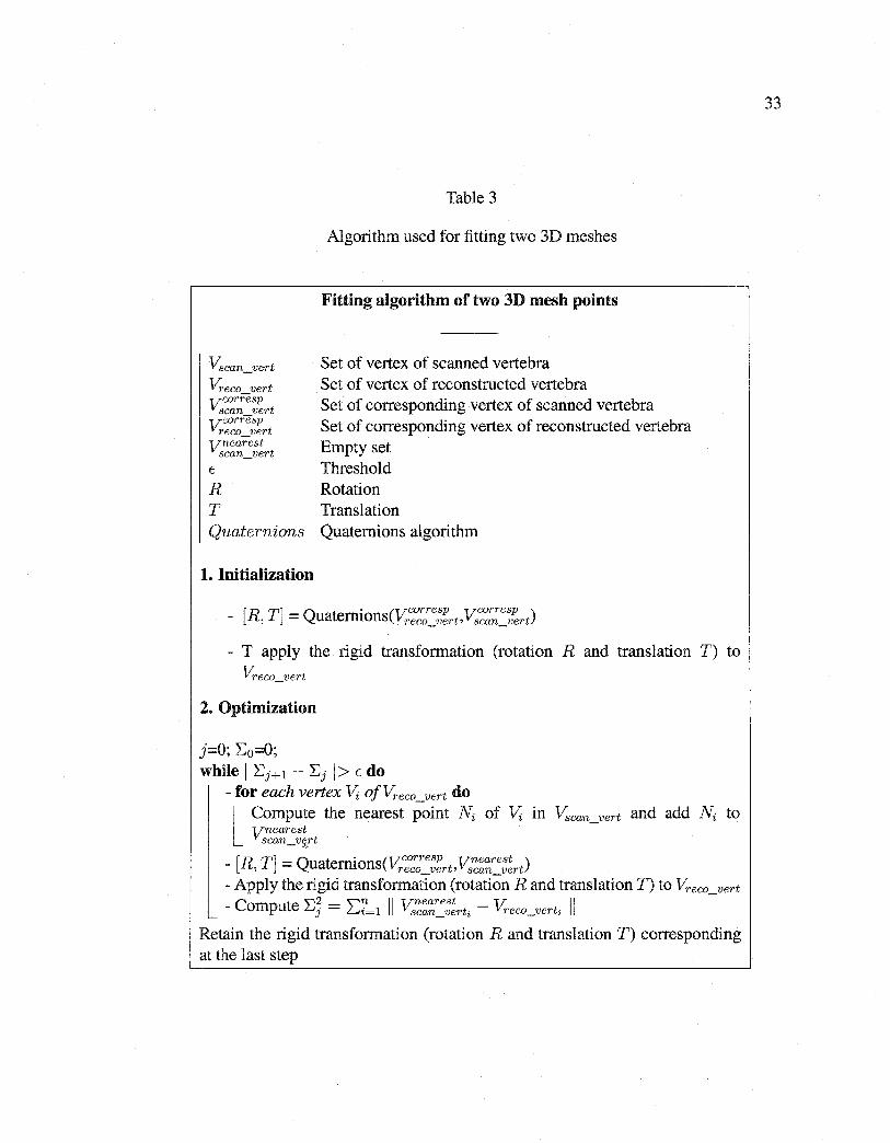
Reproduced with permission of the copyright owner. Further reproduction prohibited without permission.
"Vscan_vert
Vreco_vert
v:corresp
scan vert
v:corresp reco vert
vnearest scan_vert
E
Table 3
Algorithm used for fitting two 3D meshes
Fitting algorithm of two 3D mesh points
Set of vertex of scanned vertebra Set of vertex of reconstructed vertebra Set of corresponding vertex of scanned vertebra Set of corresponding vertex of reconstructed vertebra Empty set Threshold
R Rotation T Translation Quaternions Quaternions algorithm
1. Initialization
[R Tl _ Q · (V:corresp v:corresp ) - ' - uatemions reco_vert' scan_vert
- T apply the rigid transformation (rotation R and translation T) to
Vreco_vert
2. Optimization
j=O; :Eo=O; while 1 :EHl- :Ej 1> Edo
-for each vertex Vi ofVreco_vert do
l Compute the nearest point Ni vnearest
scan vert - t<:i
of Vi in Vscan_vert and add Ni to
[R Tl - Q t . (V:corresp vnearest ) - ' - ua emions reco_vert' scan_vert
- Apply the rigid transformation (rotation Rand translation T) to Vreco vert
-Compute :E} = L:r=l Il V:,~~~:~;rti - Vreco_verti Il -Retain the rigid transformation (rotation R and translation T) corresponding at the last step
33
Reproduced with permission of the copyright owner. Further reproduction prohibited without permission.
3.5 Experimental Results
3.5.1 Vertebra Database
34
The vertebra database consists of 1, 020 thoracic and lumbar vertebrae (510 normal and
510 scoliotic). These data were obtained by digitization of the anatomical points on
anatomical specimens. These anatomical specimens have been selected from the Hamann
Todd osteology collection of over 1, 800 complete specimens in Cleveland, USA, and from
the Robert J. Terry anatomical skeletal collection of over 1, 700 specimens at the Smith
sonian Institution in Washington, D. C., USA5. [82].
Fastrack© (POLHEMUS, A Rockwell Collins Company) is the name of the electromag
netic deviee used to digitize each vertebra by means of a pointer. The accuracy of this
deviee is evaluated at ±0.2 mm [11]. The 3D coordinates of the pointer were recorded
in a specifie reference system. The digitizing protocol consisted of measuring specifie
anatomicallandmarks on each vertebra, thus creating a set of approximately 200 points
depending on the level measured with regard to its particular geometry [88]. Different
points were acquired in a specifie order and recorded in this sequence. After the measure
ments were done, each vertebra was then reconstructed using computer graphies software.
Each set of points was then re-localized in a local coordinate system6 .
3.5.2 Radiographie Images
In our application, we used two radiographie images (i.e., postero-anterior and lateral) ac
quired with a Fuji FCR 7501S radiographie imaging system. Radiography is the image
in 2D projection of a 3D object whose X-rays are the source of illumination. The inten
sity transmitted through a specifie zone of an object varies according to the nature and
thickness of the material through which radiation passes. Thus, air, soft tissue (muscles,
cartilage, etc.) and bones present different attenuation coefficients for X-rays and can, in
5 Age, sex, race, height, weight, cause of death and peculiar dissection findings of each scoliotic specimen are available.
6To our knowledge, the vertebrae base is the largest database available in the literature [82].
Reproduced with permission of the copyright owner. Further reproduction prohibited without permission.
35
this way, become theoretically localized in radiological images. Thus, the radiographie
image illustrates the superposition of various structures on a same plane and gives place
to semi-transparent images.
3.5.3 Calibration
Calibration is a necessary step to compute the geometrical parameters of the radiologi
cal environment. The images are calibrated by a calibration object which is composed of
two acrylic sheets parallel to the X-ray film plane. The two sheets contain embedded ra
diopaque spherical markers (55 steel halls) which are easily detectable on the radiographie
images. The scene is calibrated using the 3D coordinates (X, Y, z)r of each steel ball pre
viousl y measured and the ir corresponding 2D observations (x, y) T to solve the following
equation,
(x, y, ILl= D(iJ, 11;) x (X, Y, z)r,
where IL is the x-ray tube distance, iJ and 11; being respectively the scale and rotation vector
[71]. The rotation vector iJ and the scale 11; are regrouped in the 3 x 3 dimensional matrix
D(iJ,h;).
3.5.4 Comparison Protocoi
We have validated our 3D/2D registration method on 57 scoliotic vertebrae (6 lumbar
vertebrae and 51 thoracic vertebrae) from 13 patients (13 pairs of radiographie images
(postero-anterior and lateral views) of scoliotic spines). This comparison was made using
the distance (mean, root mean square (RMS), and maximum) between a point from the
reconstructed vertebra and the surface of the corresponding vertebra obtained with CT
scan, which was considered as the ground truth and whose accuracy is ±1 mm [3].
We also considered five morphometric parameters related mostly to the dimensions of the
pedicles and the spinal canal (cf. Figure 10). These measures can be useful for the surgeon
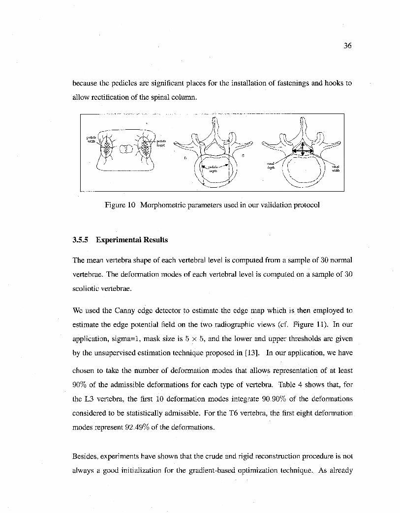
Reproduced with permission of the copyright owner. Further reproduction prohibited without permission.
36
because the pedicles are significant places for the installation of fastenings and hooks to
allow rectification of the spinal column.
p~Hiicle
h•igbt
Figure 10 Morphometric parameters used in our validation protocol
3.5.5 Experimental Results
The mean vertebra shape of each vertebrallevel is computed from a sample of 30 normal
vertebrae. The deformation modes of each vertebral level is computed on a sample of 30
scoliotic vertebrae.
We used the Canny edge detector to estimate the edge map which is then employed to
estimate the edge potential field on the two radiographie views (cf. Figure 11). In our
application, sigma=l, mask size is 5 x 5, and the lower and upper thresholds are given
by the unsupervised estimation technique proposed in [13]. In our application, we have
chosen to take the number of deformation modes that allows representation of at least
90% of the admissible deformations for each type of vertebra. Table 4 shows that, for
the L3 vertebra, the first 10 deformation modes integrate 90.90% of the deformations
considered to be statistically admissible. For the T6 vertebra, the first eight deformation
modes represent 92.49% of the deformations.
Besides, experiments have shown that the crude and rigid reconstruction procedure is not
always a good initialization for the gradient-based optimization technique. As already
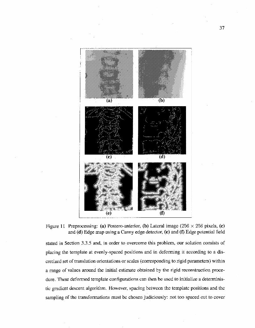
Reproduced with permission of the copyright owner. Further reproduction prohibited without permission.
37
Figure 11 Preprocessing: (a) Postero-anterior, (b) Lateral image (256 x 256 pixels, (c) and (d) Edge map using a Canny edge detector, (e) and (f) Edge potential field
stated in Section 3.3.5 and, in order to overcome this problem, our solution consists of
placing the template at evenly-spaced positions and in deforming it according to a dis
cretized set of translation orientations or scales (corresponding to rigid parameters) within
a range of values around the initial estimate obtained by the rigid reconstruction proce
dure. These deformed template configurations can then be used to initialize a determinis
tic gradient descent algorithm. However, spacing between the template positions and the
sampling of the transformations must be chosen judiciously: not too spaced out to cover
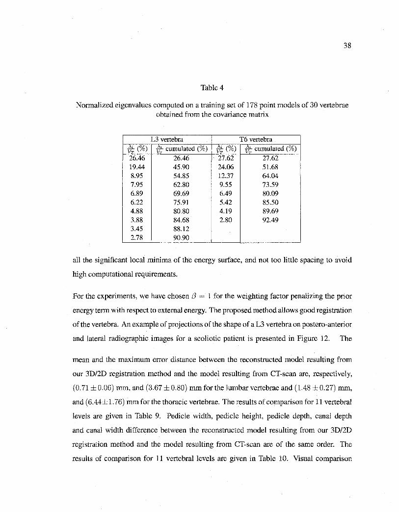
Reproduced with permission of the copyright owner. Further reproduction prohibited without permission.
38
Table 4
Normalized eigenvalues computed on a training set of 178 point models of 30 vertebrae obtained from the covariance matrix
L3 vertebra T6 vertebra * (%) v; cumulated (%) v;(%) -v; cumulated (%)
26.46 26.46 27.62 27.62 19.44 45.90 24.06 51.68 8.95 54.85 12.37 64.04 7.95 62.80 9.55 73.59 6.89 69.69 6.49 80.09 6.22 75.91 5.42 85.50 4.88 80.80 4.19 89.69 3.88 84.68 2.80 92.49 3.45 88.12 2.78 90.90
all the significant local minima of the energy surface, and not too little spacing to avoid
high computational requirements.
For the experiments, we have chosen f3 = 1 for the weighting factor penalizing the prior
energy term with respect to external energy. The proposed method allows good registration
of the vertebra. An example of projections of the shape of a L3 vertebra on postero-anterior
and lateral radiographie images for a scoliotic patient is presented in Figure 12. The
mean and the maximum error distance between the reconstructed model resulting from
our 3D/2D registration method and the model resulting from CT-scan are, respectively,
(0. 71 ± 0.06) mm, and (3.67 ± 0.80) mm for the lumbar vertebrae and (1.48 ± 0.27) mm,
and ( 6.44± 1. 76) mm for the thoracic vertebrae. The results of comparison for 11 vertebral
levels are given in Table 9. Pedicle width, pedicle height, pedicle depth, canal depth
and canal width difference between the reconstructed model resulting from our 3D/2D
registration method and the model resulting from CT-scan are of the same order. The
results of comparison for 11 vertebral levels are given in Table 10. Visual comparison
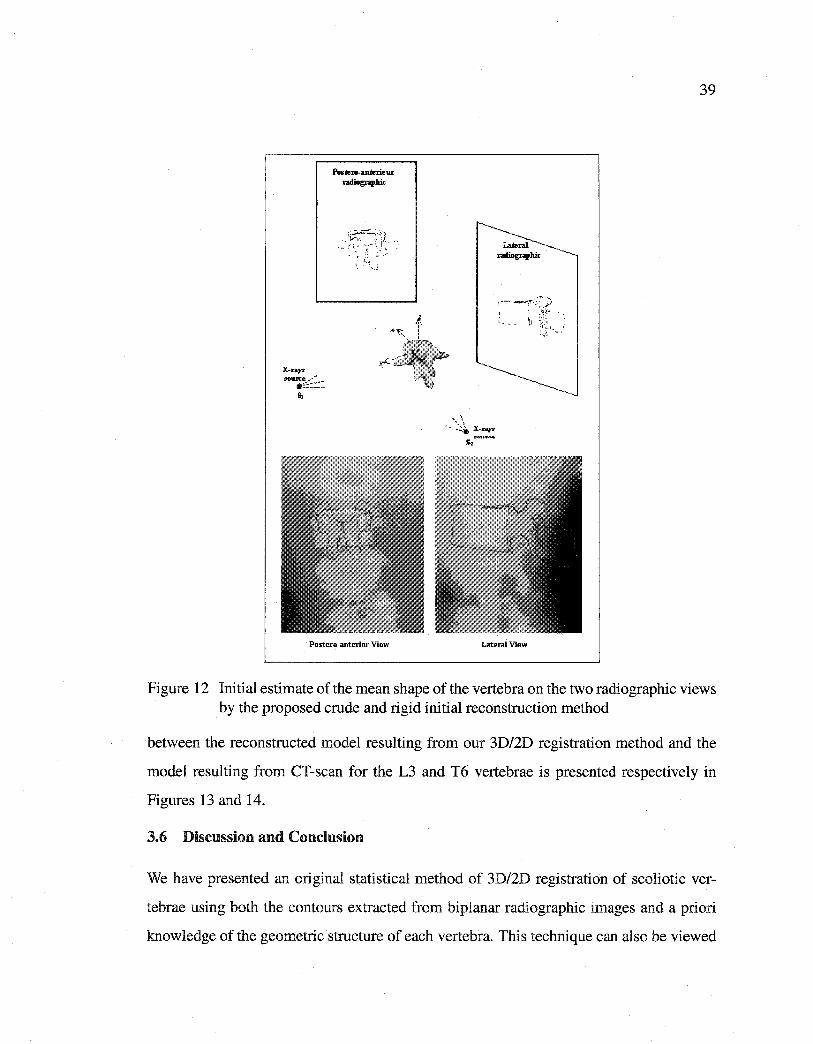
Reproduced with permission of the copyright owner. Further reproduction prohibited without permission.
X-rqs source~·""
•==:=~=s,
:. .. ·
Postero-anterior View
~ x~~ !
yJ!<~.,ri"io/P~···.
39
' ~ .~:~.:~ X-rtr;y~ 5-z ................
Lateral View
Figure 12 Initial estimate of the mean shape of the vertebra on the two radiographie views by the proposed crude and rigid initial reconstruction method
between the reconstructed model resulting from our 3D/2D registration method and the
model resulting from CT-scan for the L3 and T6 vertebrae is presented respectively in
Figures 13 and 14.
3.6 Discussion and Conclusion
We have presented an original statistical method of 3D/2D registration of scoliotic ver
tebrae using both the contours extracted from biplanar radiographie images and a priori
knowledge of the geometrie structure of each vertebra. This technique can also be viewed
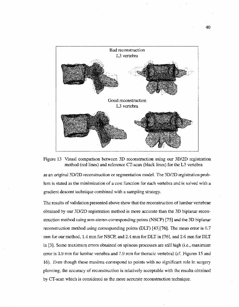
Reproduced with permission of the copyright owner. Further reproduction prohibited without permission.
Bad reconstruction L3 vertebra
Good reconstruction L3 vertebra
40
Figure 13 Visual comparison between 3D reconstruction using our 3D/2D registration method (red lines) and reference CT-scan (black lines) for the L3 vertebra
as an original 3D/2D reconstruction or segmentation model. The 3D/2D registration prob
lem is stated as the minimization of a cost function for each vertebra and is solved with a
gradient descent technique combined with a sampling strategy.
The results of validation presented above show that the reconstruction of lumbar vertebrae
obtained by our 3D/2D registration method is more accurate than the 3D biplanar recon
struction method using non-stereo-corresponding points (NSCP) [75] and the 3D biplanar
reconstruction method using corresponding points (DLT) [43][76]. The mean error is O. 7
mm for our method, 1.4 mm for NSCP, and 2.4 mm for DLT in [76], and 2.6 mm for DLT
in [3]. Sorne maximum errors obtained on spinous processes are still high (i.e., maximum
error is 3.9 mm for lumbar vertebra and 7.9 mm for thoracic vertebra) (cf. Figures 15 and
16). Even though these maxima correspond to points with no significant role in surgery
planning, the accuracy of reconstruction is relatively acceptable with the results obtained
by CT-scan which is considered as the more accurate reconstruction technique.
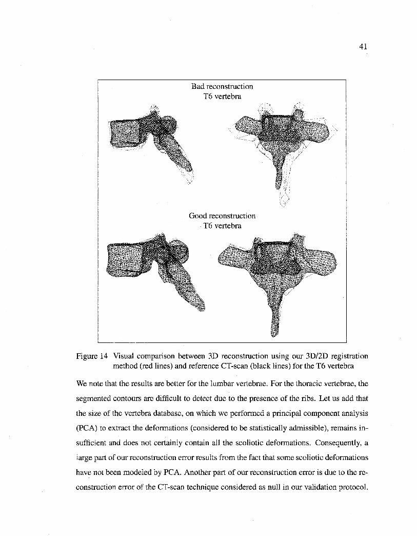
Reproduced with permission of the copyright owner. Further reproduction prohibited without permission.
Bad reconstruction T6 vertebra
Good reconstruction T6 vertebra
41
Figure 14 Visual comparison between 3D reconstruction using our 3D/2D registration method (red lines) and reference CT-scan (black lines) for the T6 vertebra
We note that the results are better for the lumbar vertebrae. For the thoracic vertebrae, the
segmented contours are difficult to detect due to the presence of the ribs. Let us add that
the size of the vertebra database, on which we performed a principal component analysis
(PCA) to extract the deformations (considered to be statistically admissible), remains in
sufficient and does not certainly contain ail the scoliotic deformations. Consequently, a
large part of our reconstruction error results from the fact that sorne scoliotic deformations
have not been modeled by PCA. Another part of our reconstruction error is due to the re
construction error of the CT-scan technique considered as null in our validation protocol.
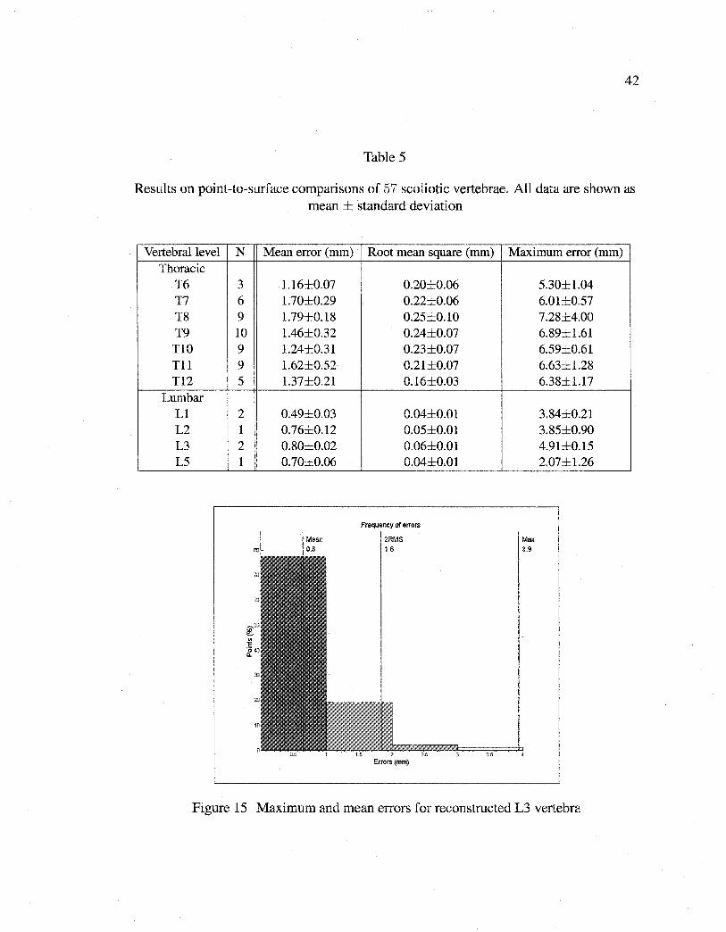
Reproduced with permission of the copyright owner. Further reproduction prohibited without permission.
42
Table 5
Results on point-to-surface comparisons of 57 scoliotic vertebrae. Ali data are shown as mean ± standard deviation
Vertebrallevel N Thoracic
T6 3 T7 6 T8 9 T9 10 TlO 9 Tl1 9 Tl2 5
Lumbar L1 2 L2 1 L3 2 L5 1
Mean error (mm) Root mean square (mm)
1.16±0.07 0.20±0.06 1.70±0.29 0.22±0.06 1.79±0.18 0.25±0.10 1.46±0.32 0.24±0.07 1.24±0.31 0.23±0.07 1.62±0.52 0.21±0.07 1.37±0.21 0.16±0.03
0.49±0.03 0.04±0.01 0.76±0.12 0.05±0.01 0.80±0.02 0.06±0.01 0.70±0.06 0.04±0.01
Frequency of errors
Errors (mm)
Maximum error (mm)
Max
3.9
5.30±1.04 6.01±0.57 7.28±4.00 6.89±1.61 6.59±0.61 6.63±1.28 6.38±1.17
3.84±0.21 3.85±0.90 4.91±0.15 2.07±1.26
Figure 15 Maximum and mean errors for reconstructed L3 vertebra
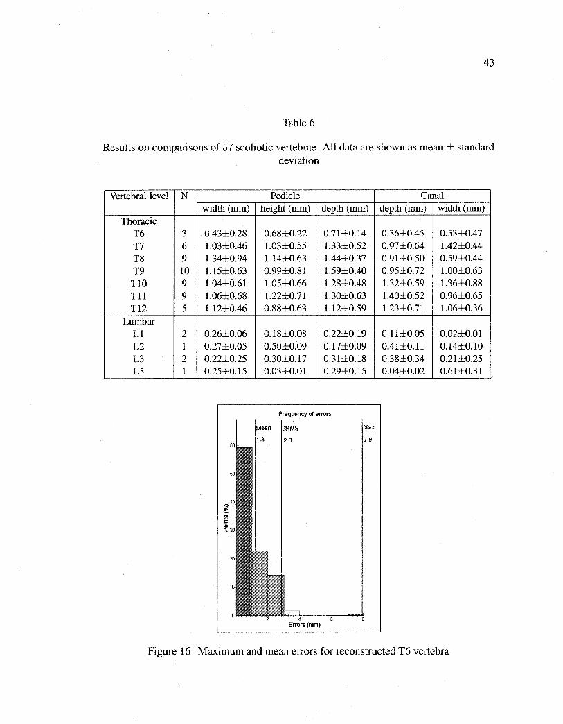
Reproduced with permission of the copyright owner. Further reproduction prohibited without permission.
43
Table 6
Results on comparisons of 57 scoliotic vertebrae. Ali data are shown as mean± standard deviation
Vertebrallevel N Pedicle Canal width (mm) height (mm) depth (mm) depth (mm) width (mm)
Thoracic T6 3 0.43±0.28 0.68±0.22 0.71±0.14 0.36±0.45 0.53±0.47 T7 6 1.03±0.46 1.03±0.55 1.33±0.52 0.97±0.64 1.42±0.44 T8 9 1.34±0.94 1.14±0.63 1.44±0.37 0.91±0.50 0.59±0.44 T9 10 1.15±0.63 0.99±0.81 1.59±0.40 0.95±0.72 1.00±0.63
TIO 9 1.04±0.61 1.05±0.66 1.28±0.48 1.32±0.59 1.36±0.88 Til 9 1.06±0.68 1.22±0.71 1.30±0.63 1.40±0.52 0.96±0.65 T12 5 1.12±0.46 0.88±0.63 1.12±0.59 1.23±0.71 1.06±0.36
Lumbar L1 2 0.26±0.06 0.18±0.08 0.22±0.19 0.11±0.05 0.02±0.01 L2 1 0.27±0.05 0.50±0.09 0.17±0.09 0.41±0.11 0.14±0.10 L3 2 0.22±0.25 0.30±0.17 0.31±0.18 0.38±0.34 0.21±0.25 L5 1 0.25±0.15 0.03±0.01 0.29±0.15 0.04±0.02 0.61±0.31
Frequency of errors
2.6 .9
4 Errors (mm)
Figure 16 Maximum and mean errors for reconstructed T6 vertebra
Reproduced with permission of the copyright owner. Further reproduction prohibited without permission.
44
Nevertheless, we can observe that the results obtained for morphometric parameters are
nearly comparable with those obtained by CT-scan. Let us mention that these parameters
are important for the surgical correction of scoliosis.
Let us recall that the surgical correction of scoliosis consists of correcting the scoliotic
deformation by rotations and translations practiced at the level of the vertebrae and/or the
level of the spine until a more normal alignment of the vertebrae is obtained. Correction
consists of fixing the spine in this configuration using a metal rod supported by hooks and
screws installed in the pedicles. Knowledge of the accurate sizes and geometry of these
pedicles is thus crucial.
Let us note that the estimated global deformation parameters after reconstruction (i.e.,
parameter vector b, setting the amplitude of each deformation mode of the scoliotic defor
mations) and the measures of morphometric parameters can also be used to quantify the
scoliosis, its nature orto analyze the improvement of orthopedie or surgical corrections.
To conclude, this method has demonstrated its efficiency and robustness. We strongly
believe that a method which gives results almost equal to those obtained by using more
than 500 CT images for a whole spine but based on only two standard X-ray images is
quite original, important, and interesting. It is interesting for the quantity of data to be
acquired, processed and managed. For example, two plain digital Fuji X-rays require
15 Mbytes (1, 760 x 2, 140 x 2 bytes) of storage in comparison to 260 Mbytes (512 x
512 x 2 bytes x500 slices). It is important for the quantity of radiation receîved by the
patient. With the generalization of multi-detector spiral CT, patients will be more and
more exposed to radiation and a method that can keep this amount of radiation as low as
possible is also quite important and has to be considered. It becomes especially important
when we deal with young scoliotic patients who will be exposed to multiple diagnostic
radiographie examinations during their childhood and adolescence. In [34], a retrospective
study confirmed that multiple radiographie examinations may increase the risk of breast
cancer among women with scoliosis. Another important point is that scoliosis must be

Reproduced with permission of the copyright owner. Further reproduction prohibited without permission.
45
evaluated when the patient is in a standing position, which is impossible with standard CT
scanners.
The proposed method remains sufficiently general to be applied to other medical recon
struction problems (i.e., rib cage, pelvis, knee, etc.) for which the database of this anatom
ical structure is available (with two or several radiographie views). We now intend to
improve the proposed method by integrating a region homogeneity term in the energy
function related to this statistical reconstruction approach, to refine the statistical model
by local deformations, and to use a more efficient global optimization technique.
Reproduced with permission of the copyright owner. Further reproduction prohibited without permission.
RECONSTRUCTION 3D BIPLANAIRE NON SUPERVISÉE DE LA COLONNE VERTÉBRALE SCOLIOTIQUE PAR
APPROCHE STATISTIQUE HIÉRARCHIQUE
46
Article : A hierarchical statistical modeling approach for the unsupervised 3D bipla
nar reconstruction of the scoliotique spine.
Cet article a été soumis au journal IEEE Transactions on Biomedical Engineering comme
l'indique la référence bibliographique
S. Benameur, M. Mignotte, H. Labelle, J. A. De Guise. A hierarchical statistical modeling
approache for the unsupervised 3D biplanar reconstruction of the scoliotic spine. IEEE
Transactions on BioMedical Engineering, soumis, 2004.
Cet article est présenté ici dans sa version originale.
Résumé
La reconstruction 3D des structures osseuses à partir d'un nombre limité d'images radio
graphiques conventionnelles est l'un des axes importants de recherche en vision et image
rie médicale. La majorité des méthodes existantes dans la littérature sont supervisées et/ou
ne s'appliquent pas aux cas pathologiques (cas de la scoliose) [7] [39]. Nous présentons
dans cet article une méthode non supervisée, hiérarchique et statistique de reconstruction
3D de la colonne vertébrale scoliotique à partir de deux vues radiographiques convention
nelles (postéro-antérieure avec incidence de 0° et latérale) calibrées. La méthode présen
tée utilise les contours des vertèbres segmentées dans les deux vues radiographiques et
une connaissance globale hiérarchique a priori comprenant la structure géométrique de
la colonne vertébrale et de chaque niveau vertébral. La méthode proposée est basée sur
les spécifications de deux modèles 3D statistiques. Le premier, un modèle géométrique
sur lequel des déformations linéaires globales admissibles sont définies, est utilisé pour
une reconstruction grossière de la colonne vertébrale. Une reconstruction 3D précise est
Reproduced with permission of the copyright owner. Further reproduction prohibited without permission.
47
alors réalisée pour chaque niveau vertébral par un deuxième modèle de vertèbre sur le
quel des déformations non linéaires admissibles et des déformations locales sont définies
à partir d'une base d'apprentissage d'environ 1, 000 vertèbres (30 vertèbres saines et 30
vertèbres scoliotiques par niveau vertébral). Cette reconstruction 3D est formulée comme
un double problème de minimisation de fonction d'énergie. Cette minimisation est réalisée
par un algorithme stochastique d'exploration/sélection [79]. La méthode proposée est va
lidée sur une base de 57 vertèbres lombaires et thoraciques de 13 patients scoliotiques qui
ont aussi été reconstruites par CT-scan pour des fins de comparaison. Une erreur moyenne
de (1.45±1.46) mm pourles vertèbres lombaires et de (1.27±1.29) mm pourles vertèbres
thoraciques obtenue sur les distances point-surface entre le modèle reconstruit avec notre
méthode et le modèle issu de la reconstruction CT-scan. La reconstruction 3D nécessite un
temps de calcul de 1' ordre de 28 secondes pour une vertèbre (sur un PC/Linux à 2. 0 GHz).
Reproduced with permission of the copyright owner. Further reproduction prohibited without permission.
CHAPITRE4
A HIERARCHICAL STATISTICAL MODELING APPROACH FOR THE UNSUPERVISED 3D BIPLANAR RECONSTRUCTION
OF THE SCOLIOTIC SPINE
Abstract This paper presents a new and accurate 3D reconstruction technique for the scoliotic spine from a pair of planar and conventional (postero-anterior with normal in-
cidence and lateral) calibrated radiographie images. The proposed model uses a priori
hierarchical global knowledge, both on the geometrie structure of the whole spine and
of each vertebra. More precisely, it relies on the specification of two 3D statistical tem
plates. The first, a rough geometrie template on which rigid admissible deformations are
defined, is used to ensure a crude registration of the whole spine. An accurate 3D recon
struction is then performed for each vertebra by a second template on which non-linear
admissible global, as weil as local deformations, are defined. Global deformations are
modeled using a statistical modal analysis of the pathological deformations observed on
a representative scoliotic vertebra population. Local deformations are represented by a
first order Markov process. This unsupervised coarse-to-fine 3D reconstruction procedure
leads to two separate minimization procedures efficiently solved in our application with
evolutionary stochastic optimization algorithms. In this context, we compare the results
obtained with a classical Genetic Algorithm (GA) and a recent Exploration Selection (ES)
technique. This latter optimization method with the proposed 3D reconstruction model,
is tested on several pairs of biplanar radiographie images with scoliotic deformities. The
experiments reported in this paper demonstrate that the discussed method is comparable
in terms of accuracy with the classical CT-scan technique while being unsupervised and
while requiring only two radiographie images and a lower amount of radiation for the
patient.
Reproduced with permission of the copyright owner. Further reproduction prohibited without permission.
49
Key words: 3D reconstruction model, 3D/2D registration, hierarchical statistical mod
eling, shape model, biplanar radiographies, scoliosis, medical imaging, energy function
minimization, stochastic optimization.
4.1 Introduction
In the past few years, there has been a great deal of research in reconstructing three
dimensional (3D) shapes of anatomical structures from radiographie images. In medical
imagery, this 3D reconstruction problem remains a necessary step to obtain qualitative
information, such as the detection of pathological deformations, as well as for quantitative
measurements needed for surgical planing and follow-up evaluation. In this paper, we are
concemed with computer vision methods for 3D reconstruction of scoliotic spine, from
two X-ray radiographie images.
Scoliosis is a complex 3D deformity of the natural curve of the spinal column, includ
ing rotations and vertebral deformations. The classical evaluation obtained by the spinal
projections on the two-dimensional (2D) radiographie planar images does not give a full
and accurate interpretation of scoliotic deformities [15]. To analyze the 3D characteristics
of these deformations, several 3D reconstruction methods have been developed. Among
these methods, the 3D reconstruction methods of tomodensitometric imagery modalities
(e.g., computerized tomography [61][62], or magnetic resonance [65][87]) provide ac
curate 3D information of the human anatomy or 4D information including time as one
more degree of freedom. However, few hospitals can afford a magnetic resonance sys
tem. Efficient and affordable tomodensitometric imagery systems can now be found in
every hospital and many clinics but for ethical reasons hazardous X-ray dosages cannat
be used extensively enough to provide full 3D data or large bone structures as the spine
or rib cage. Also, these medical imaging techniques require that the patient be in a lying
position, which is incompatible with many diagnostic protocols evaluating scoliosis.
For these above-mentioned reasons, a 3D reconstruction method of shapes using a limited
number of X-ray radiographie projections and thus ensuring a lower amount of radiation
Reproduced with permission of the copyright owner. Further reproduction prohibited without permission.
50
for the patient, is really interesting. Surprisingly, this problem has not been widely studied
in the statistical framework, and few references exist in the computer vision and medical
imagery literature. Among the proposed algorithmic technique, we can cite the 3D re
construction method from silhouettes, proposed by Martin and Aggarwal in [70]. Their
method allows to reconstruct polygonal 3D objects by back-projecting the silhouettes. A
method for extracting 3D geometry ofbones from two orthogonal X-ray radiographie pro
jections is also proposed by Caponetti and Fanelli in [14]. The initial estimation of the
3D bone structure, produced by back-projecting profile points, is then refined by using
a B-spline interpolation. In [9], Benjamin generates surface information using common
points, present in different projections, and the tracks between the points, extracted from
about ten projection images.
Due to the ill-posed nature of this reconstruction problem, a right and accurate estimation
of the 3D geornetrical structure of the shape cannat be found without constraints. In this
way, methods using simple a priori knowledge on the geometrical structure of the abject to
be reconstructed, and thus expressed as the solution of a regularized inverse problem, have
been proposed. Terzopoulos et al. propose in [90] a method allowing to recover the 3D
shape from the 3D profiles of an abject using, as geometrie prior constraint, a deformable
tube coupled to a deformable spine. The deformation is controlled by physically-based in
ternai and external forces. Bardinet et al. present in [4] a method that consists in matching
a parametric deformable model to unstructured 3D data. More precisely, a super-quadric
model is fitted to a given point set, and the generated super-quadric model is deformed
locally using free-form deformations. In [78], Nikkhade et al. present 3D reconstruction
method of femurs from two orthogonal X-ray radiographie projections. They separate the
femur into three subparts; each of them assumed to be round. They fit cubic parametric
surface patches to the subparts and then assemble them to a complete model. Kit devel
ops in [57] a method allowing to analyze X-ray radiographie projections of the stomach
using a deformable 3D rnodel. Their a priori rnodel is a tube which is first initialized
using only one projection. Afterward, the model is deformed using the other projections.
Reproduced with permission of the copyright owner. Further reproduction prohibited without permission.
51
Nevertheless, in these methods, the geometrie a priori constraint does not madel the set
of admissible deformation (or in the case of scoliosis, the pathological variability) of the
anatomical structure to be reconstructed. Consequently, the 3D reconstructed shape esti
mation does not necessarily correspond to the reality.
In arder to rightly constraint the ill-posed nature of this problem, a solution consists in
supervising the 3D reconstruction technique. In this sense, a 3D multiplanar radiogra
phy reconstruction method using a direct linear transformation (DLT) [71] is presented by
Dansereau and Stokes in [24]. They rely on manual stereo-digitization of six anatomical
landmarks (on each X-ray radiographie image) of the vertebrae to produce 3D coordi
nates. Adding the kriging technique using the 3D reconstructed points as control points
yields good visualization of the vertebral geometry [28]. There is a need for more land
marks to obtain a better description of ali the vertebrae. In the same way, a non-stereo
corresponding points technique is also described by Mitton et al. in [75] to improve the
accuracy of the 3D reconstruction by identifying more anatomicallandmarks on the X -ray
projections. This method is then based on deformation of an elastic deformable mesh that
respects stereo corresponding and non-stereo corresponding points available in different
X-ray radiographie projections. In addition to the supervision, the methods proposed by
Dansereau et al., Mitton et al. and Delorme et al. are limited due to the inherent inac
curacy produced in identifying anatomicallandmarks (leading to reconstruction errors).
Besides, they do not exploit all information contained in the two X-ray radiographie pro
jections (e.g., the contours of each vertebra) or the statistical knowledge of the possible
deformation of the abject to be reconstructed.
Methods using statistical a priori knowledge of the geometrie shapes of the abjects of
interest lead to better constrain the reconstruction problem. In [39], Fleute and Laval
lée propose a method allowing to reconstruct the 3D geometry of the femur using a few
orthogonal X-ray radiographie projections. They apply point distribution models (PDM)
[18] to reconstruct a geometrie prior madel representing mean shapes and containing the
Reproduced with permission of the copyright owner. Further reproduction prohibited without permission.
52
typical deformation modes in statistical sense. Thereafter, they deform the model non
rigidly, according to the rays back-projected from the contour points of the projections
taken from a patient. Benameur et al. proposed in [7] a 3D statistical reconstruction
method, for each individual vertebra, using a pair of planar and conventional (postero
anterior with normal incidence and lateral) radiographie images for a patient in standing
position, and a prior global knowledge of the geometrie structure of each vertebra. The
method consists of fitting the projections of this deformable template with the prelim
inary segmented contours of the corresponding vertebra on the two X -ray radiographie
projections. Nevertheless the above-mentioned technique remains widely supervised and
requires the knowledge of the position of six anatomical points (namely, the center of
the superior and inferior end-plates, the upper and lower extremities of both pedicles) to
initialize 3D reconstruction process of each vertebra of the spine.
To overcome this problem of supervision and improve the 3D reconstruction and the op
timizer related to the energy-based model presented in [7], we propose in this paper a 3D
statistical reconstruction method based on the likelihood introduced in [7] but using hier
archical global a priori knowledge on the geometrie structure of both the whole spine and
each vertebra1• More precisely, the hierarchical model we propose relies on the specifica
tion of two 3D templates. The first, a rough and cubic approximation geometrie template
on which rigid admissible deformations are defined, is used to fit its (postero-anterior and
lateral) projections with the preliminary segmented contours of each vertebra body of the
spine on the two calibrated radiographie views. It ensures erode registration of the whole
spine and gives a rough position and orientation of each vertebra. 3D reconstruction is then
refined by a second template which takes into account a priori global knowledge on the
geometrie structure of each vertebra. This geometrie knowledge is efficiently captured by
a statistical deformable template integrating a set of admissible deformations, expressed
1Hierarchical statistical models have been applied in fusion of multiresolution image data [58], segmentation [55], restoration [60], in active shape models using the wavelet transform [25]. To our knowledge, no hierarchical statistical model for 3D reconstruction methods have been described in the literature.
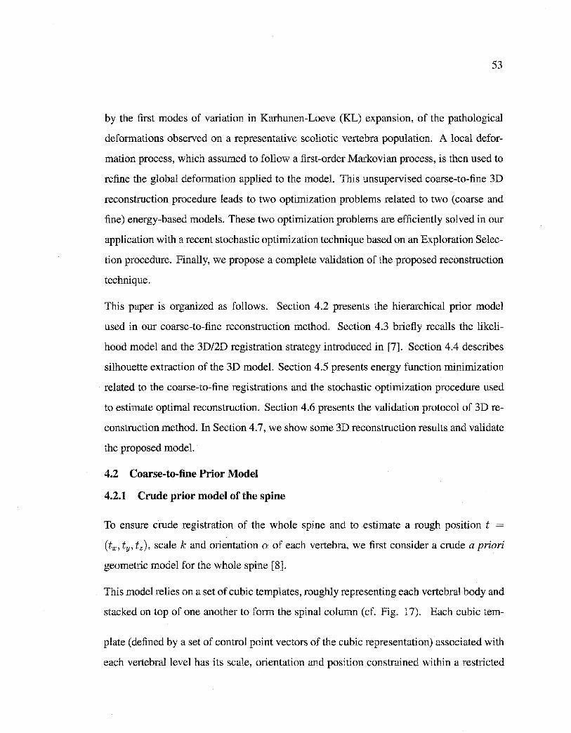
Reproduced with permission of the copyright owner. Further reproduction prohibited without permission.
53
by the first modes of variation in Karhunen-Loeve (KL) expansion, of the pathological
deformations observed on a representative scoliotic vertebra population. A local defor
mation process, which assumed to follow a first-order Markovian process, is then used to
refine the global deformation applied to the model. This unsupervised coarse-to-fine 3D
reconstruction procedure leads to two optimization problems related to two ( coarse and
fine) energy-based models. These two optimization problems are efficiently solved in our
application with a recent stochastic optimization technique based on an Exploration Selec
tion procedure. Finally, we propose a complete validation of the proposed reconstruction
technique.
This paper is organized as follows. Section 4.2 presents the hierarchical prior model
used in our coarse-to-fine reconstruction method. Section 4.3 briefiy recalls the likeli
hood model and the 3D/2D registration strategy introduced in [7]. Section 4.4 describes
silhouette extraction of the 3D model. Section 4.5 presents energy function minimization
related to the coarse-to-fine registrations and the stochastic optimization procedure used
to estimate optimal reconstruction. Section 4.6 presents the validation protocol of 3D re
construction method. In Section 4. 7, we show sorne 3D reconstruction results and validate
the proposed model.
4.2 Coarse-to-fine Prior Model
4.2.1 Crude prior model of the spine
To ensure crude registration of the whole spine and to estimate a rough position t
(tx, ty, tz), scale k and orientation a of each vertebra, we first considera crude a priori
geometrie model for the whole spine [8].
This model relies on a set of cubic templates, roughly representing each vertebral body and
stacked on top of one another to form the spinal column (cf. Fig. 17). Bach cubic tem-
plate (defined by a set of control point vectors of the cubic representation) associated with
each vertebrallevel has its scale, orientation and position constrained within a restricted
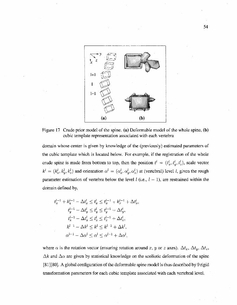
Reproduced with permission of the copyright owner. Further reproduction prohibited without permission.
54
r\y y x z cg 1+1 []
1-1 g ~ (a) (b)
Figure 17 Crude prior model of the spine. (a) Defonnable model of the whole spine, (b) cubic template representation associated with each vertebra
domain whose center is given by knowledge of the (previously) estimated parameters of
the cubic template which is located below. For example, if the registration of the whole
erode spine is made from bottom to top, then the position t1 = (t;, tt, t;), scale vector
k1 = (k;, k;, k~) and orientation(} = (a~, at, a~) at (vertebral) levell, given the rough
parameter estimation of vertebra below the levell (i.e., l - 1), are restrained within the
domain defined by,
tl-1 + kl-1 - fltl < tl < tl-1 + kl-1 + fltl X X X- X - X X Xl
tl-1 - fltl < tl < tl-1 + fltl y y - y- y Y'
tl-1 - fltl < tl < tl-1 + fltl Z Z - Z - Z Zl
where ais the rotation vector (ensuring rotation around x, y or z axes). lltx, flty, lltz,
llk and .6.a are given by statistical knowledge on the scoliotic deformation of the spine
[81][80]. A global configuration of the defonnable spine model is thus described by 9 rigid
transformation parameters for each cubic template associated with each vertebrallevel.
Reproduced with permission of the copyright owner. Further reproduction prohibited without permission.
55
4.2.2 Fine prior model of each vertebra
Our a priori knowledge model relies also on the description of each vertebra by a 3D de
formable template (i.e., a vector s E R 3n of n control points) which incorporates statistical
knowledge about its geometrical structure and its pathological variability. The deforma
tions of this template are expressed by the first modes of variation in KL expansion of
pathological deformations observed on a representative training scoliotic vertebra popula
tion [7]. This can be done by using principal component analysis (PCA), i.e., by comput
ing the covariance matrix C of shapes {si}. The main deformation modes of the template
model sare then described by the eigenvectors 4> of C, with the largest eigenvalues >.(cf.
Fig. 18).
4.2.2.1 Deformable template representation
The shape s is represented as a template, that is a set of points
where Pi = (xi, Yi, zi) T are the Cartesian coordinates of each surface point.
Given a sample s 1 ,. ··,sn of shapes with the same number of points, we resort to the pro
cedure proposed in [50] to align this training set. We then apply the PCA to reduce the
dimension tom << 3n. This gives us non-linear deformations of the mean shape sand
terminates the training phase.
4.2.2.2 Global deformations
The globally deformed template is defined by,
s = M(k, a)[s +<Pb]+ T, (4.1)
where,
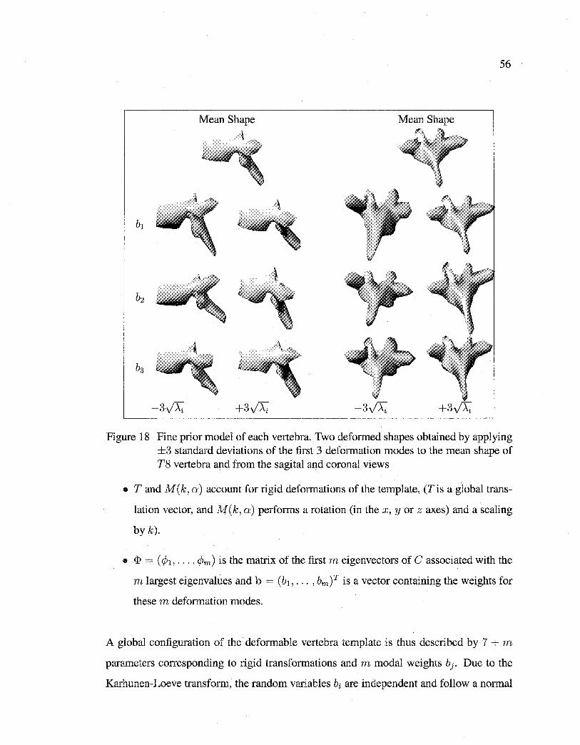
Reproduced with permission of the copyright owner. Further reproduction prohibited without permission.
56
Mean Shape Mean Shape c\
,
Figure 18 Fine prior model of each vertebra. Two deformed shapes obtained by applying ±3 standard deviations of the first 3 deformation modes to the mean shape of T8 vertebra and from the sagital and corona! views
• T and M ( k, a) account for rigid deformations of the template, (T is a global trans
lation vector, and M(k, a) performs a rotation (in the x, y or z axes) and a scaling
by k).
• <I> = ( (h, ... , 4Ym) is the matrix of the fust m eigenvectors of C associated with the
m largest eigenvalues and b = (b1 , ... , bm)T is a vector containing the weights for
these m deformation modes.
A global configuration of the deformable vertebra template is thus described by 7 + m
parameters corresponding to rigid transformations and m modal weights bj. Due to the
Karhunen-Loeve transform, the random variables bi are independent and follow a normal
Reproduced with permission of the copyright owner. Further reproduction prohibited without permission.
57
law of a null mean and variance Ài. Thus, the law of probability of s(O), the deformed
template, can be written as [7],
m 1 ( b2) P(s(B)) = U(T, k, a) I1 ~exp --f- , i=l 2Ài1f 2Ai
(4.2)
where U denotes the uniform distribution. This low parametric representation for each
vertebra level, along with the erode parametric representation of the whole spinal column
constitutes our global hierarchical a priori model that will be used to rightly constrain the
ill-posed nature of our proposed coarse-to-fine 3D reconstruction method.
The a priori energy term related to the prior distribution (Bq. 4.2), can be written as,
(4.3)
which is close to the Mahalonobis distance. This prior energy term penalizes the deviation
of the deformed template from the mean shape (but not the affine transformations).
4.2.2.3 Local deformations
Inspired by the work of Grenander and Keenan on stochastic pattern representation [42],
a statisticallocal deformations process b is now applied to the n control points or "land
marks" which approximate the geometrical shape of each vertebra.
These local deformations are modeled as local random perturbations of the shape and can
be considered as a refinement of the global deformations applied to the deformed mean
shape, since the main deformation modes have already been captured by the prelirninary
global statistical prior knowledge of each vertebra. The local deformation vector b =
(b1 , b2 , ... , bn)T with bi = (bxi' Oyi, Ozi) is described by a first order Gauss-Markov process
defined on the graph corresponding to the n control points of the deformable template of
each vertebra. If we represent these local deformations by local random translations (that
Reproduced with permission of the copyright owner. Further reproduction prohibited without permission.
58
are superimposed on the globall y deformed shape), the complete (i.e., globall y and loc ali y)
deformable model of each vertebra can be defined by,
s = M(k, a)[s + <I>b] + T +b. (4.4)
In our application, this local deformation process allows to take into account firstly, the
fact that our PCA does not model 100% of the scoliotic deformations of our vertebra
database (the first m deformation modes are chosen in order to get a reasonably low para
metric representation model) and secondly the fact that our vertebra database could not be
big or representative enough and consequent! y could not certainly contain ali the possible
scoliotic deformations. Assuming a first-order neighborhood structure on the graph asso
ciated to the n control points of the deformable template, the probability distribution of
the random field b can be written as,
1 P(b) = (exp ( -Er(b)),
where ( is a normalization constant, and Er ( b) is the local deformation energy term which
can be written as,
(4.5)
where N(i) is the set of first-order neighborhood of point i, f-lt and vf are the variance
parameters of this local deformation model. f-lT weight the interactions between neighbor
ing points. vf control the amplitude of the local deformations compared to the globally
deformed model. In our application, we consider /-li = f-l and vi = v, Vi, since the different
control points of our 3D vertebra template are approximative! y equally spaced.
Reproduced with permission of the copyright owner. Further reproduction prohibited without permission.
59
4.3 Likelihood Model
As proposed in [7], the likelihood model is expressed by a measure of similarity between
the external contour of the (postero-anterior and the lateral) projections of the 3D deformed
template and a directional edge potential field estimated on the two radiographie views.
This likelihood energy term is defined by,
(4.6)
where the summation of the first and second term of E1 is overall the nPA and nLAT points of
the external contour of the respecti v el y lateral ( hAr) and postero-anterior ( I pA) perspec
tive projections of the deformed template on the two pre-computed edge potential fields
of each radiographie image. The 2D perspective projections of the 3D deformed template,
i.e., the lateral and postero-anterior outline is computed with the silhouette extraction al
gorithm.
To compute the edge potential field 'li associated with each radiographie view, we first
use a Canny edge detector with the unsupervised technique proposed in [13]. Then, 'li is
defined as in [53] by,
(4.7)
where Ç = (Çx, f,y) is the displacement to the nearest edge point in the image, and Tisa
smoothing factor which controls the degree of smoothness of this potential field. 1 (x, y) is
the angle between the tangent of the nearest edge and the tangent direction of the contour
at (x, y) (cf. Fig. 19). This likelihood energy term, as expressed in Bq. (4.4), is exploited
for the 3D reconstruction of the fine prior model of each vertebra (see subsection 4.2.2).
In order to ensure a good reconstruction of each cube template of the crude prior model
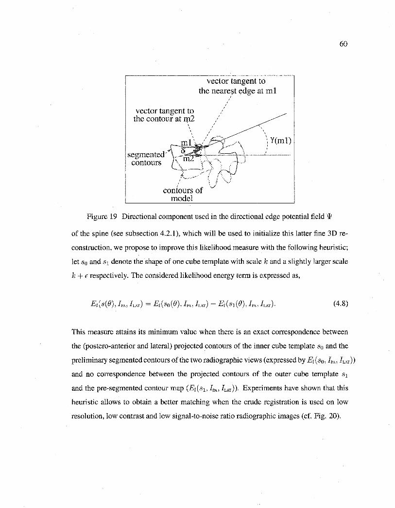
Reproduced with permission of the copyright owner. Further reproduction prohibited without permission.
vector tangent to the neare~t edge at ml
vector tangent to the contour at :q12
\
' \ \
' ' ' '
' ' ' '
' '
' ' \
ml\ / \ Y(ml)
segmented'~~~ .r-' .·.,-_.-. --=:::=.-+-..;.._---'-: --
contours C:~_-.J' \ ' '
contours of mode!
Figure 19 Directional component used in the directional edge potential field w
60
of the spine (see subsection 4.2.1), which will be used to initialize this latter fine 3D re
construction, we propose to improve this likelihood measure with the following heuristic;
let s0 and s 1 denote the shape of one cube template with scale k and a slightly larger scale
k + E respectively. The considered likelihood energy term is expressed as,
(4.8)
This measure attains its minimum value when there is an exact correspondence between
the (postero-anterior and lateral) projected contours of the inner cube template s0 and the
preliminary segmentedcontours of the tworadiographic views (expressed by Ez(s0 , IPA' !LAT))
and no correspondence between the projected contours of the outer cube template s1
and the pre-segmented contour map (Ez(s 1 , IPA' !LAT)). Experiments have shown that this
heuristic allows to obtain a better matching when the crude registration is used on low
resolution, low contrast and low signal-to-noise ratio radiographie images (cf. Fig. 20).
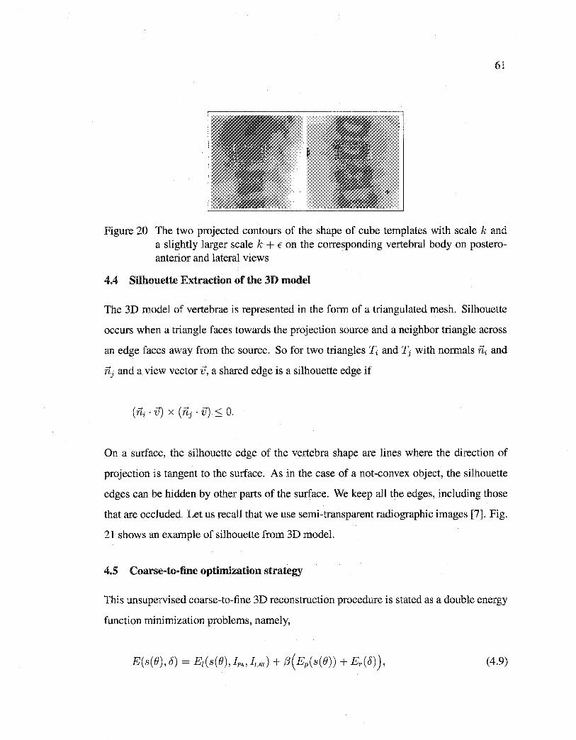
Reproduced with permission of the copyright owner. Further reproduction prohibited without permission.
61
Figure 20 The two projected contours of the shape of cube templates with scale k and a slightly larger scale k + E on the corresponding vertebral body on posteroanterior and lateral views
4.4 Silhouette Extraction of the 3D model
The 3D model of vertebrae is represented in the form of a triangulated mesh. Silhouette
occurs when a triangle faces towards the projection source and a neighbor triangle across
an edge faces away from the source. So for two triangles ~ and Tj with normals ni and
iïj and a view vector iJ, a shared edge is a silhouette edge if
On a surface, the silhouette edge of the vertebra shape are lines where the direction of
projection is tangent to the surface. As in the case of a not-convex object, the silhouette
edges can be hidden by other parts of the surface. We keep all the edges, including those
that are occluded. Let us recall that we use semi-transparent radiographie images [7]. Fig.
21 shows an example of silhouette from 3D model.
4.5 Coarse-to-fine optimization strategy
This unsupervised coarse-to-fine 3D reconstruction procedure is stated as a double energy
function minimization problems, namely,
(4.9)
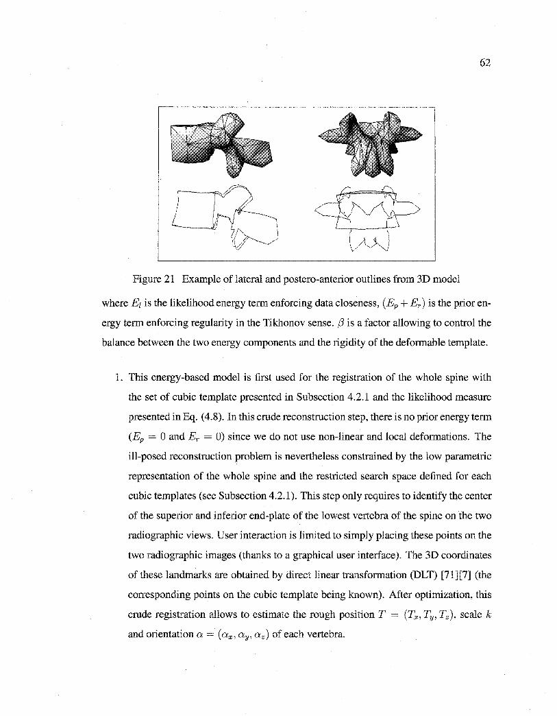
Reproduced with permission of the copyright owner. Further reproduction prohibited without permission.
62
Figure 21 Example of lateral and postero-anterior outlines from 3D model
where El is the likelihood energy term enforcing data closeness, ( Ep + Er) is the prior en
ergy term enforcing regularity in the Tikhonov sense. j3 is a factor allowing to control the
balance between the two energy components and the rigidity of the deformable template.
1. This energy-based model is first used for the registration of the whole spine with
the set of cubic template presented in Subsection 4.2.1 and the likelihood measure
presented in Eq. ( 4.8). In this eructe reconstruction step, there is no prior energy term
(Ep = 0 and Er = 0) since we do not use non-linear and local deformations. The
ill-posed reconstruction problem is nevertheless constrained by the low parametric
representation of the whole spine and the restricted search space defined for each
cubic templates (see Subsection 4.2.1). This step only requires to identify the center
of the superior and inferior end-plate of the lowest vertebra of the spine on the two
radiographie views. User interaction is limited to simply placing these points on the
two radiographie images (thanks to a graphical user interface). The 3D coordinates
of these landmarks are obtained by direct linear transformation (DLT) [71][7] (the
corresponding points on the cubic template being known). After optimization, this
crude registration allows to estimate the rough position T = (Tx, Ty, Tz), scale k
and orientation a= (ax, ay, o:2 ) of each vertebra.
Reproduced with permission of the copyright owner. Further reproduction prohibited without permission.
63
2. This optimization problem is then used with the fine prior template of each vertebra
(see Subsection 4.2.2) and the likelihood measure proposed in Eq. (4.4) in two steps.
(a) Optimization is made within a range of values around the rigid parameters
roughly estimated by the first crude reconstruction given in step 1. In this step,
we consider the local deformations as negligible (Ji = 0, Vi) and we have
to estimate e = (k, a, T, b), i.e., 7 + m parameters corresponding to rigid
transformations and m modal weights bi.
(b) Finally, a last minimization procedure is made with B previously estimated and
now fixed to find the optimal local deformation parameters of the complete
model.
The energy functions to be minimized in Step 1 and 2 are complex with several local
minima over the deformation parameter space. A global search is impossible due to the
size of the configuration space. Let us also add that the quality of the reconstruction is
closely related to the good estimation of the deformation parameters and consequently to
the performance of the optimization procedure. In our application, we use the stochastic
optimization algorithm recently proposed by O. François in [79]. We use this algorithm
because the adjustment of all internai parameters does not depend on the function to be
minimized. Moreover, the convergence is asymptotically ensured [79]. Let us add that
this optimization algorithm is also especially weil suited to minimize complex (i.e., non
convex) energy functions [32]. We compare the performance of this algorithm, in Section
4.7.3, with a classical genetic algorithm [74].
4.5.1 Exploration/Selection Algorithm
The E/S algorithm belongs to the class of Evolutionary algorithms. This class of algorithm
has been successfully applied in diverse areas such as medical imaging [74], localization
of shapes [32] to minimize complex energy functions [32]. This success has initiated
the development of various evolutionary algorithm variants and stimulated the theoretica]
Reproduced with permission of the copyright owner. Further reproduction prohibited without permission.
64
research about convergence properties of these algorithms (see [84] for a good review of
evolutionary algorithm in medical imagery).
The E/S algorithm can be summarized as follows (more details are given in [79]); Let F
be a finite discrete subset of the Cartesian product of k compact intervals [mi, Mi], for
1 ::::; i ::::; k, and () = { B1 , ... , Bn} a set of n potential solutions randomly chosen. We
define ê as the optimal element (Ji of() such that E(s(BJ)) > E(s(Bï)), for 1 ::::; j < i,
and E(s(BJ)) 2 E(s(Bi)), for 1 < j ::::; n. We considera graph G defined on F called the
exploration graph. The exploration graph is assumed to be non-oriented and connected.
We denote by N (a) the neighborhood of the element a E F in the graph G defined by
{bEF: for sorne j, lbJ - aJI ::::; r(MJ-mJ), bi =ai, i:;i= j} where ris a real number in the
interval [0,1] called the radius of exploration.
Each solution of () is regarded as an individual that attempts a random search on the ex
ploration graph [79]. For b E F, we fix a positive distribution ab on N ( b). The exploration
process acts independently on each individual, and consists of choosing a random N ac
cording to the binomial distribution bin(n, p) where n is the size of the population and p
is the probability of exploration. We replace (Ji by {) i EN ((Ji)\ {Ô} according to a uniform
distribution, for i::::; N otherwise, we change (Ji by ê. This process is runs until a criterion
is met (see Table 7).
Finally, the energy function to be minimized in Step 2.2 is just a final refinement of the
global deformations applied to the mean shape, since the main deformation modes have
been captured by the PCA-based global prior knowledge of each vertebra. For this step,
we use the following deterministic procedure,
• For each points Pi of the vertebra shape model s ( s = (p1 , p2 , ... Pi, ... l Pn) T with
Pi= (xi Yi zif), and until E (s(B)) is stable,
• The model energy E (s(B)), expressed by Eq. (4.9) is evaluated for different po
sitions of Pi (namely; Pi+ 8pi, Pi, and Pi - 8pi) along its normal. The normal is
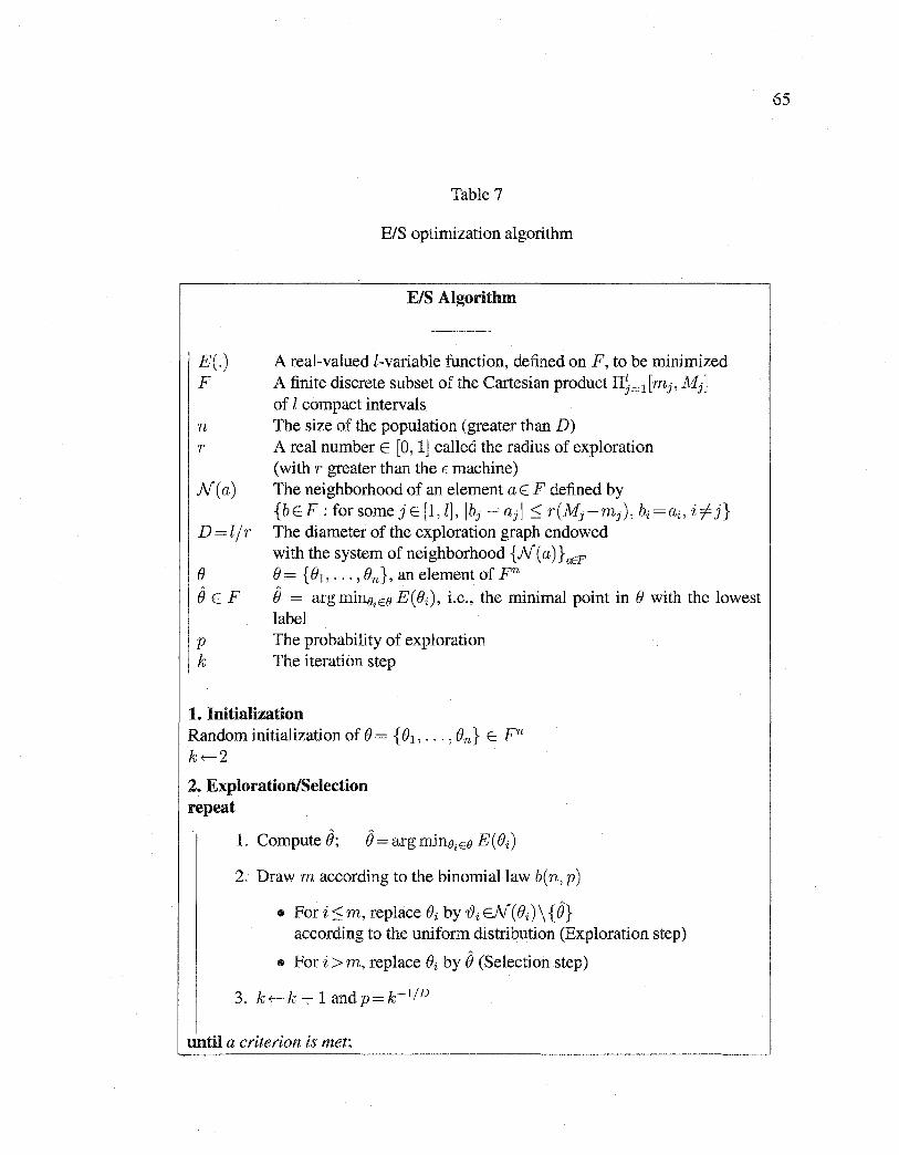
Reproduced with permission of the copyright owner. Further reproduction prohibited without permission.
Table 7
E/S optirnization algorithm
E/S Algorithm
E(.) A real-valued Z-variable function, defined on F, to be rninirnized F A finite discrete subset of the Cartesian product II~=1 [mj, Mj]
of l compact intervals n The size of the population (greater than D) r A real number E [0, 1] called the radius of exploration
( with r greater than the E machine) N (a) The neighborhood of an element a E F defined by
{bEF: for sorne jE [1, Z], lbj- ajl :::; r(Mj -mj), bi =ai, i=;tf j} D = l / r The diameter of the exploration graph endowed
with the system of neighborhood {N (a)} aEF
e e= { e1, ... , en}, an element of Fn Ô E F Ô = argmino;EO E(ei), i.e., the minimal point in e with the lowest
label p The probability of exploration k The iteration step
1. Initialization Random initialization of e= {e1 , ... , en} E Fn k+-2
2. Exploration/Selection repeat
1. Compute ê; Ô=argmino;EO E(ei)
2. Draw m according to the binomial law b( n, p)
• Fori:::;m, replace ei by'!9iEN(ei)\{Ô} according to the uniform distribution (Exploration step)
• For i > m, replace ei by ê (Selection step)
3. k+-k + 1 andp=k-1/D
until a criterion is met;
65
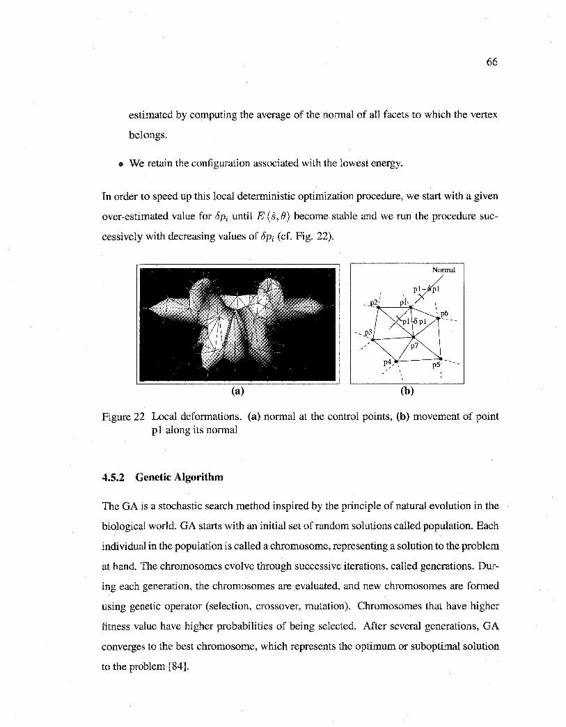
Reproduced with permission of the copyright owner. Further reproduction prohibited without permission.
66
estimated by computing the average of the normal of ali facets to which the vertex
be longs.
e We retain the configuration associated with the lowest energy.
In arder to speed up this local deterministic optimization procedure, we start with a given
over-estimated value for rSpi until E ( .§, B) become stable and we run the procedure suc
cessive! y with decreasing values of rSpi (cf. Fig. 22).
Normal
(b)
Figure 22 Local deformations. (a) normal at the control points, (b) movement of point pl along its normal
4.5.2 Genetic Algorithm
The GA is a stochastic search method inspired by the principle of natural evolution in the
biological world. GA starts with an initial set of random solutions called population. Bach
individual in the population is called a chromosome, representing a solution to the problem
at hand. The chromosomes evolve through successive iterations, called generations. Dur
ing each generation, the chromosomes are evaluated, and new chromosomes are formed
using genetic operator (selection, crossover, mutation). Chromosomes that have higher
fitness value have higher probabilities of being selected. After several generations, GA
converges to the best chromosome, which represents the optimum or suboptimal solution
to the problem [84].
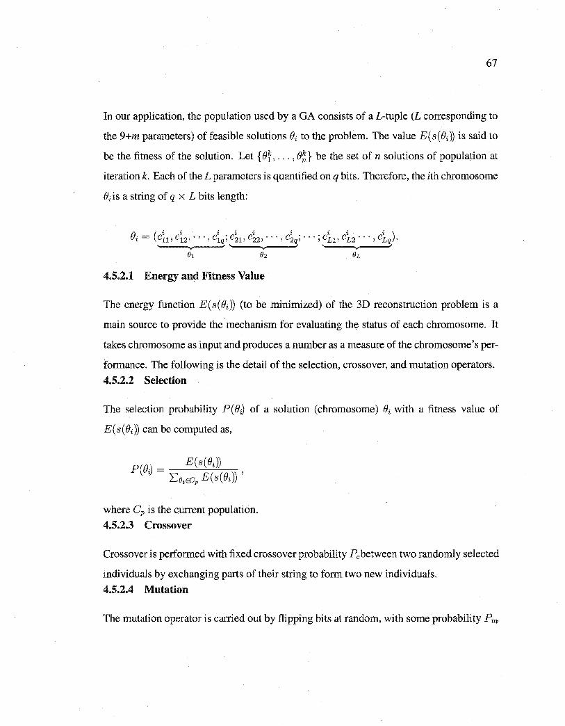
Reproduced with permission of the copyright owner. Further reproduction prohibited without permission.
67
In our application, the population used by a GA consists of a L-tuple (L corresponding to
the 9+m parameters) of feasible solutions ()i to the problem. The value E(s(Bi)) is said to
be the fitness of the solution. Let { ()~, ... , ()~} be the set of n solutions of population at
iteration k. Each of theL parameters is quantified on q bits. Therefore, the ith chromosome
()i is a string of q x L bits length:
4.5.2.1 Ene:rgy and Fitness Value
The energy function E(s(Bi)) (to be minimized) of the 3D reconstruction problem is a
main source to provide the mechanism for evaluating the status of each chromosome. It
takes chromosome as input and produces a number as a measure of the chromosome's per
formance. The following is the detail of the selection, crossover, and mutation operators.
4.5.2.2 Selection
The selection probability P(Bi) of a solution (chromosome) ()i with a fitness value of
E(s(Bi)) can be computed as,
where Cp is the current population.
4.5.2.3 C:rossove:r
Crossover is performed with fixed crossover probability Pcbetween two randomly selected
individuals by exchanging parts of their string to form two new individuals.
4.5.2.4 Mutation
The mutation operator is carried out by fiipping bits at random, with sorne probability Pm
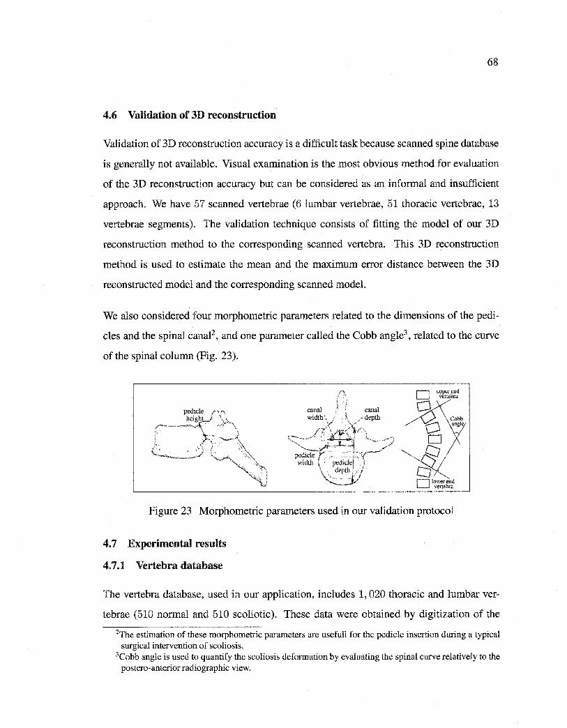
Reproduced with permission of the copyright owner. Further reproduction prohibited without permission.
68
4.6 Validation of 3D reconstruction
Validation of 3D reconstruction accuracy is a difficult task because scanned spine database
is generally not available. Visual examination is the most obvious method for evaluation
of the 3D reconstruction accuracy but can be considered as an informai and insufficient
approach. We have 57 scanned vertebrae (6 lumbar vertebrae, 51 thoracic vertebrae, 13
vertebrae segments). The validation technique consists of fitting the model of our 3D
reconstruction method to the corresponding scanned vertebra. This 3D reconstruction
method is used to estimate the mean and the maximum error distance between the 3D
reconstructed model and the corresponding scanned model.
We also considered four morphometric parameters related to the dimensions of the pedi
cles and the spinal canal2 , and one parameter called the Cobb angle3 , related to the curve
of the spinal column (Fig. 23).
Figure 23 Morphometric parameters used in our validation protocol
4. 7 Experimental results
4. 7.1 Vertebra database
The vertebra database, used in our application, includes 1, 020 thoracic and lumbar ver
tebrae (510 normal and 510 scoliotic). These data were obtained by digitization of the
2The estimation of these morphometric parameters are usefull for the pedicle insertion during a typical surgical intervention of scoliosis.
3Cobb angle is used to quantify the scoliosis deformation by evaluating the spinal curve relatively to the postero-anterior radiographie view.
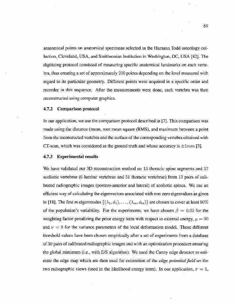
Reproduced with permission of the copyright owner. Further reproduction prohibited without permission.
69
anatomical points on anatomical specimens selected in the Hamann Todd osteology col
lection, Cleveland, USA, and Smithsonian Institution in Washington, DC, USA [82]. The
digitizing protocol consisted of measuring specifie anatomical landmarks on each verte
bra, thus creating a set of approximately 200 points depending on the level measured with
regard to its particular geometry. Different points were acquired in a specifie order and
recorder in this sequence. After the measurements were done, each vertebra was then
reconstructed using computer graphies.
4. 7.2 Comparison protocol
In our application, we use the comparison protocol described in [7]. This comparison was
made using the distance (mean, root mean square (RMS), and maximum between a point
from the reconsructed vertebra and the surface of the corresponding vertebra obtained with
CT-scan, which was considered as the ground truth and whose accuracy is ±lmm [3].
4. 7.3 Experimental results
We have validated our 3D reconstruction method on 13 thoracic spine segments and 57
scoliotic vertebrae (6 lumbar vertebrae and 51 thoracic vertebrae) from 13 pairs of cali
brated radiographie images (postero-anterior and lateral) of scoliotic spines. We use an
efficient way of calculating the eigenvectors associated with non zero eigenvalues as given
in [ 18]. The first m eigenmodes { (À 1 , (PI), ... , ( Àm, <Pm)} are chosen to cover at least 90%
of the population's variability. For the experiments, we have chosen f3 = 0.02 for the
weighting factor penalizing the prior energy term with respect to extemal energy, fJ = 90
and v = 8 for the variance parameters of the local deformation model. These different
threshold values have been chosen empirically after a set of experiments from a database
of 30 pairs of calibrated radiographie images and with an optimization procedure ensuring
the global minimum (i.e., with E/S algorithm). We used the Canny edge detector to esti
mate the edge map which are then used for estimation of the edge potential field on the
two radiographie views (used in the likelihood energy term). In our application, 0' = 1,
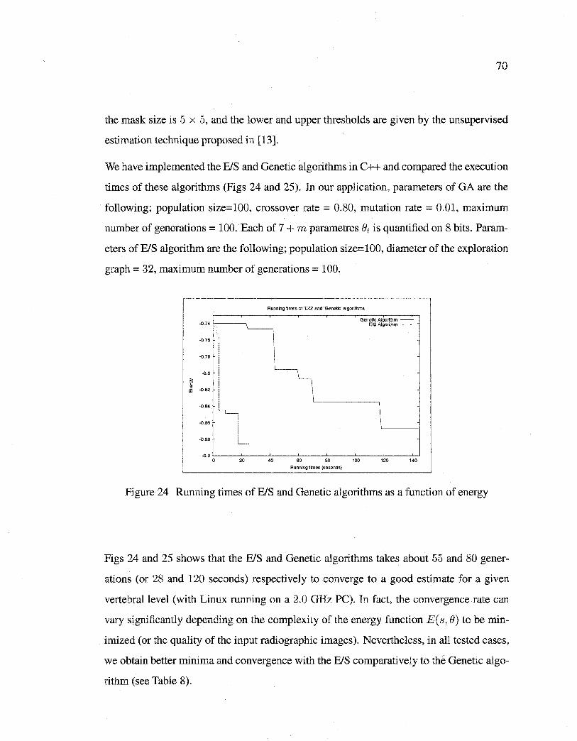
Reproduced with permission of the copyright owner. Further reproduction prohibited without permission.
70
the mask size is 5 x 5, and the lower and upper thresholds are given by the unsupervised
estimation technique proposed in [13].
We have implemented the BIS and Genetic algorithms in C++ and compared the execution
times of these algorithms (Figs 24 and 25). In our application, parameters of GA are the
following; population size=100, crossover rate = 0.80, mutation rate = 0.01, maximum
number of generations = 100. Bach of 7 + m parametres ei is quanti:fied on 8 bits. Param
eters of BIS algorithm are the following; population size=100, diameter of the exploration
graph = 32, maximum number of generations= 100.
-0.74
T -0.76
-0.78
·0.8
El . Ji -0.82
-0.84
-0.86
-0.88 '-----
-0.9 0 20
Running times of 'EIS' and 'Genetic' algorithms
40 60 80
Running times (seconds)
100
Genaüc Algorithm -E!S Algorithm -------
120 140
Figure 24 Running times of BIS and Genetic algorithms as a function of energy
Figs 24 and 25 shows that the BIS and Genetic algorithms takes about 55 and 80 gener
ations (or 28 and 120 seconds) respectively to converge to a good estimate for a given
vertebrallevel (with Linux running on a 2.0 GHz PC). In fact, the convergence rate can
vary signi:ficantly depending on the complexity of the energy function E(s, e) to be min
imized (or the quality of the input radiographie images). Nevertheless, in all tested cases,
we obtain better minima and convergence with the B/S comparative! y to the Genetic algo
rithm (see Table 8).
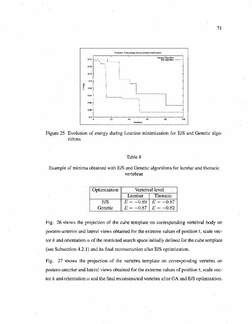
Reproduced with permission of the copyright owner. Further reproduction prohibited without permission.
Evolution of the energy during function mînimization
'-----------------.., __________________ \
: :
Genetic Atgorithm -EIS Algorithm -------
1
\ _______________________________________________ _
.0.9 L,_ __ _,_ ___ ,__ __ _,_ ___ ..__ __ _j
0 20 40 60 80 100
Iterations
71
Figure 25 Evolution of energy during function rninimization for E/S and Genetic algorithms
Table 8
Example of minima obtained with E/S and Genetic algorithms for lumbar and thoracic vertebrae
Optimization Vertebral level Lumbar Thoracic
E/S E = -0.89 E = -0.87 Genetic E = -0.87 E = -0.82
Fig. 26 shows the projection of the cube template on corresponding vertebral body on
postero-anterior and lateral views obtained for the extreme values of position t, scale vec
tor k and orientation a of the restricted search space initially defined for the cube template
(see Subsection 4.2.1) and its final reconstruction after E/S optirnization.
Fig. 27 shows the projection of the vertebra template on corresponding vertebra on
postero-anterior and lateral views obtained for the extreme values of position t, scale vec
tor k and orientation a and the final reconstructed vertebra after GA and E/S optimization.
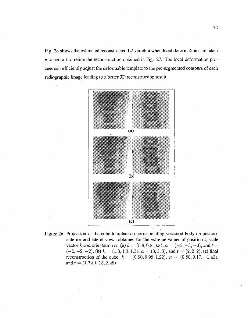
Reproduced with permission of the copyright owner. Further reproduction prohibited without permission.
72
Fig. 28 shows the estimated reconstructed L2 vertebra when local deformations are taken
into acount to refine the reconstruction obtained in Fig. 27. The local deformation pro
cess can efficiently adjust the deformable template to the pre-segmented contours of each
radiographie image leading to a better 3D reconstruction result.
Figure 26 Projection of the cube template on corresponding vertebral body on posteroanterior and lateral views obtained for the extreme values of position t, scale vector k and orientation a. (a) k = (0.8, 0.8, 0.8), a= ( -3, -3, -3), and t =
( -2, -2, -2), (b) k = (1.3, 1.3, 1.3), a = (3, 3, 3), and t = (2, 2, 2), (c) final reconstruction of the cube, k = (0.90, 0.98, 1.22), a = (0.80, 0.17, -1.42), and t = (1.72, 0.13, 2.28)
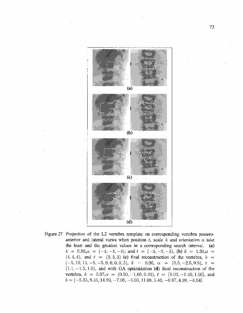
Reproduced with permission of the copyright owner. Further reproduction prohibited without permission.
73
(d) .
Figure 27 Projection of the L2 vertebra template on corresponding vertebra posteroanterior and lateral views when position t, scale k and orientation a: take the least and the greatest values in a corresponding search interval. (a) k = 0.86,o: = ( -4, -4, -4), and t = ( -3, -3, -3), (b) k = 1.30,o: -(4, 4, 4), and t = (3, 3, 3) (c) final reconstruction of the vertebra, b = ( -5, 10, 15, -5, -5, 0, 0, 0, 0, 5), k = 0.96, 0: = (0.5, -2.5, 0.5), t = (1.1, -1.5, 1.0), and with GA optimization (d) final reconstruction of the vertebra, k = 0.97,o: = (0.50, -1.05, 0.49), t = (1.03, -1.49, 1.00), and b = ( -5.35, 8.45, 14.69, -7.06, -5.05, 11.08, 5.43, -0.87, 4.10, -6.64)
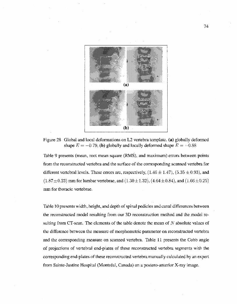
Reproduced with permission of the copyright owner. Further reproduction prohibited without permission.
74
(a)
Figure 28 Global and local deformations on L2 vertebra template. (a) globally deformed shape E = -0.79, (b) globally and locally deformed shape E = -0.88
Table 9 presents (mean, root mean square (RMS), and maximum) errors between points
from the reconstructed vertebra and the surface of the corresponding scanned vertebra for
different vertebrallevels. These errors are, respectively, (1.46 ± 1.47), (5.35 ± 0.93), and
(1.87±0.23) mmforlumbarvertebrae, and (1.30±1.32), (4.64±0.84), and (1.66±0.25)
mm for thoracic vertebrae.
Table 10 presents width, height, and depth of spinal pedicles and canal differences between
the reconstructed model resulting from our 3D reconstruction method and the model re
sulting from CT-scan. The elements of the table denote the mean of N absolute values of
the difference between the measure of morphometric parameter on reconstructed vertebra
and the corresponding measure on scanned vertebra. Table 11 presents the Cobb angle
of projections of vertebral end-plates of these reconstructed vertebra segments with the
corresponding end-plates of these reconstructed vertebra manually calculated by an expert
from Sainte-Justine Hospital (Montréal, Canada) on a postero-anterior X-ray image.
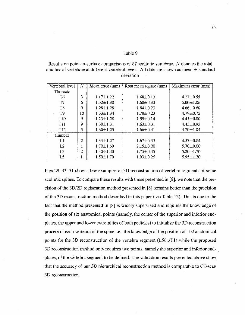
Reproduced with permission of the copyright owner. Further reproduction prohibited without permission.
75
Table 9
Results on point-to-surface comparisons of 57 scoliotic vertebrae. N denotes the total number of vertebrae at different vertebrallevels. All data are shown as mean± standard
deviation
Vertebral leve! N Mean error (mm) Root mean square (mm) Maximum error (mm) Thoracic
T6 3 1.17±1.22 1.48±0.13 4.27±0.55 T7 6 1.32±1.38 1.68±0.33 5.00±1.06 T8 9 1.28±1.28 1.64±0.23 4.66±0.60 T9 10 1.33±1.34 1.70±0.23 4.79±0.75 TIO 9 1.23±1.28 1.59±0.14 4.41±0.80 Til 9 1.30±1.31 1.63±0.31 4.43±0.95 T12 5 1.30±1.25 1.66±0.41 4.20±1.04
Lumbar LI 2 1.33±1.27 1.67±0.33 4.57±0.84 L2 1 1.70±1.60 2.15±0.00 5.70±0.00 L3 2 1.30±1.30 1.75±0.35 5.20±1.70 L5 1 1.50±1.70 1.93±0.25 5.95±1.20
Figs 29, 33, 31 show a few examples of 3D reconstruction of vertebra segments of sorne
scoliotic spines. To compare these results with those presented in [8], we note that the pre
cision of the 3D/2D registration method presented in [8] remains better than the precision
of the 3D reconstruction method described in this paper (see Table 12). This is due to the
fact that the method presented in [8] is widely supervised and requires the knowledge of
the position of six anatomical points (namely, the center of the superior and inferior end
plates, the upper and lower extremities of both pedicles) to initialize the 3D reconstruction
process of each vertebra of the spine i.e., the knowledge of the position of 102 anatomical
points for the 3D reconstruction of the vertebra segment (L5/ ... /T1) while the proposed
3D reconstruction method only requires two points, namely the superior and inferior end
plates, of the vertebra segment to be defined. The validation results presented above show
that the accuracy of our 3D hierarchical reconstruction method is comparable to CT-scan
3D reconstruction.
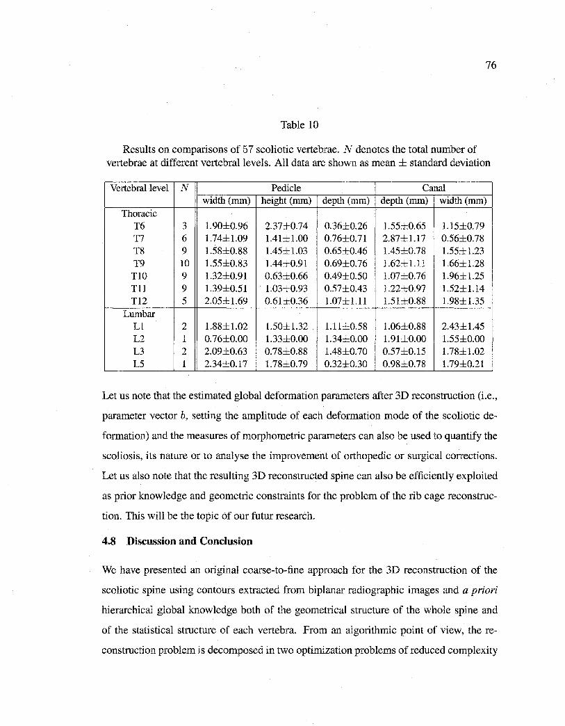
Reproduced with permission of the copyright owner. Further reproduction prohibited without permission.
76
Table 10
Results on comparisons of 57 scoliotic vertebrae. N denotes the total number of vertebrae at different vertebrallevels. Ali data are shown as mean ± standard deviation
Vertebrallevel N Pedicle Canal width (mm) height (mm) depth (mm) depth (mm) width (mm)
Thoracic T6 3 1.90±0.96 2.37±0.74 0.36±0.26 1.55±0.65 1.15±0.79 T7 6 1.74±1.09 1.41±1.00 0.76±0.71 2.87±1.17 0.56±0.78 T8 9 1.58±0.88 1.45±1.03 0.65±0.46 1.45±0.78 1.55±1.23 T9 10 1.55±0.83 1.44±0.91 0.69±0.76 1.62±1.11 1.66±1.28
TlO 9 1.32±0.91 0.63±0.66 0.49±0.50 1.07±0.76 1.96±1.25 Tll 9 1.39±0.51 1.03±0.93 0.57±0.43 1.22±0.97 1.52±1.14 T12 5 2.05±1.69 0.61±0.36 1.07±1.11 1.51±0.88 1.98±1.35
Lumbar Ll 2 1.88±1.02 1.50±1.32 1.11±0.58 1.06±0.88 2.43±1.45 L2 1 0.76±0.00 1.33±0.00 1.34±0.00 1.91±0.00 1.55±0.00 L3 2 2.09±0.63 0.78±0.88 1.48±0.70 0.57±0.15 1.78±1.02 L5 1 2.34±0.17 1.78±0.79 0.32±0.30 0.98±0.78 1.79±0.21
Let us note that the estimated global deformation parameters after 3D reconstruction (i.e.,
parameter vector b, setting the amplitude of each deformation mode of the scoliotic de
formation) and the measures of morphometric parameters can also be used to quantify the
scoliosis, its nature or to analyse the improvement of orthopedie or surgical corrections.
Let us also note that the resulting 3D reconstructed spine can also be efficiently exploited
as prior knowledge and geometrie constraints for the problem of the rib cage reconstruc
tion. This will be the topic of our futur research.
4.8 Discussion and Conclusion
We have presented an original coarse-to-fine approach for the 3D reconstruction of the
scoliotic spine using contours extracted from biplanar radiographie images and a priori
hierarchical global knowledge both of the geometrical structure of the whole spine and
of the statistical structure of each vertebra. From an algorithmic point of view, the re
construction problem is decomposed in two optimization problems of reduced complexity
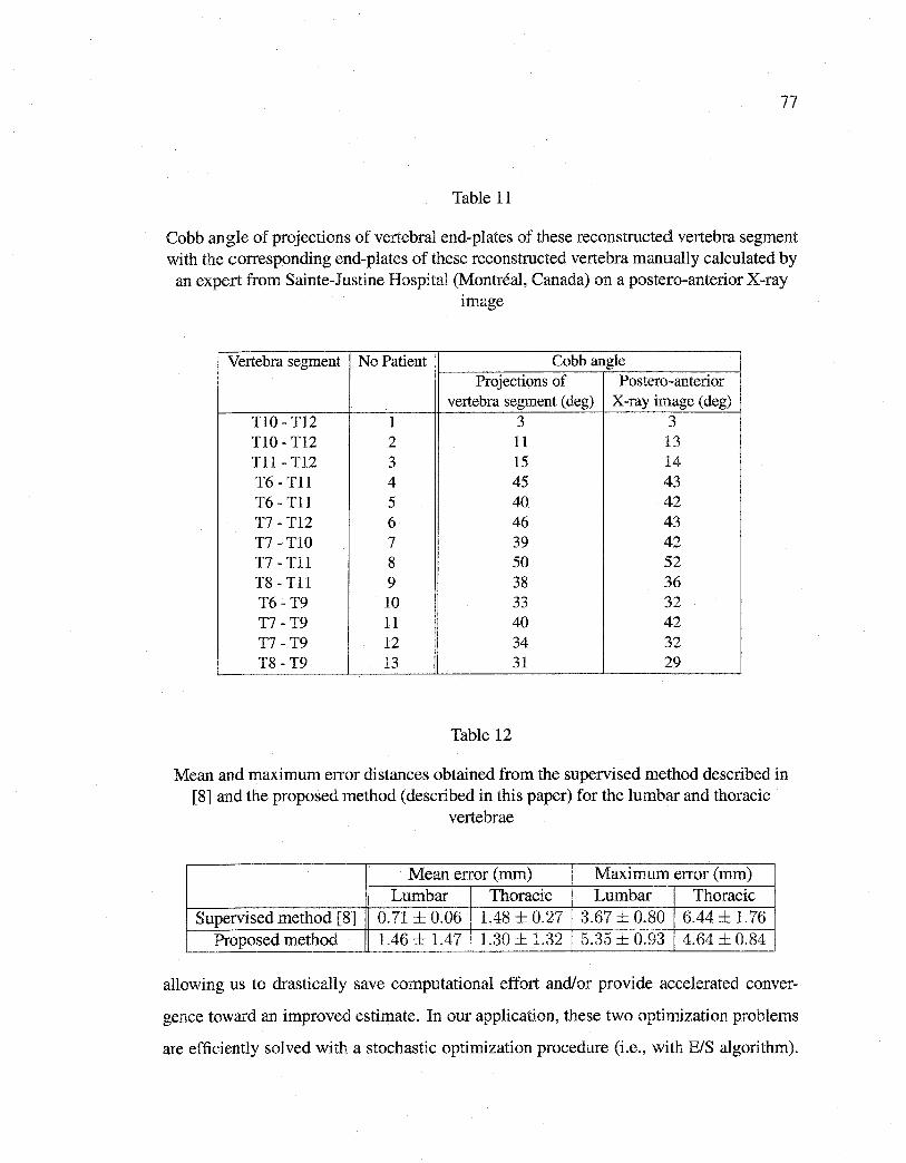
Reproduced with permission of the copyright owner. Further reproduction prohibited without permission.
77
Table 11
Cobb angle of projections of vertebral end-plates of these reconstructed vertebra segment with the corresponding end-plates of these reconstructed vertebra manually calculated by
an expert from Sainte-Justine Hospital (Montréal, Canada) on a postero-anterior X-ray image
Vertebra segment No Patient Cobb angle Projections of Postero-anterior
vertebra segment ( deg) X-ray image (deg) TIO- T12 1 3 3 TlO- Tl2 2 11 13 Tll- T12 3 15 14 T6- Tll 4 45 43 T6- Tll 5 40 42 T7- T12 6 46 43 T7- TlO 7 39 42 T7- Tll 8 50 52 T8- Tll 9 38 36 T6- T9 10 33 32 T7 -T9 11 40 42 T7 -T9 12 34 32 T8 -T9 13 31 29
Table 12
Mean and maximum error distances obtained from the supervised method described in [8] and the proposed method (described in this paper) for the lumbar and thoracic
vertebrae
Mean error (mm) Maximum error (mm) Lumbar Thoracic Lumbar Thoracic
Supervised method [8] 0.71 ± 0.06 1.48 ± 0.27 3.67 ± 0.80 6.44 ± 1.76 Proposed method 1.46 ± 1.47 1.30 ± 1.32 5.35 ± 0.93 4.64 ± 0.84
allowing us to drastically save computational effort and/or provide accelerated conver
gence toward an improved estimate. In our application, these two optimization problems
are efficiently solved with a stochastic optimization procedure (i.e., with BIS algorithm).
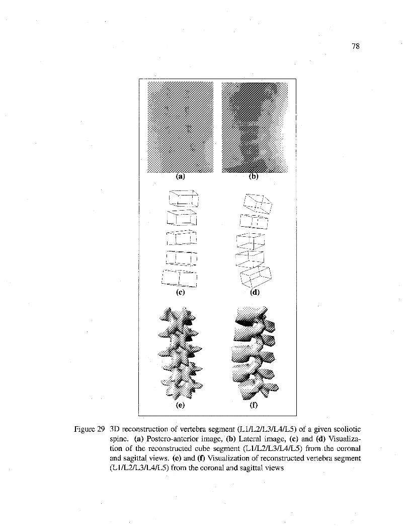
Reproduced with permission of the copyright owner. Further reproduction prohibited without permission.
lLlJ co
(c)
(e)
78
(f)
Figure 29 3D reconstruction of vertebra segment (Ll/L2/L3/IAIL5) of a given scoliotic spine. (a) Postero-anterior image, (b) Lateral image, (c) and (d) Visualization of the reconstructed cube segment (Ll/L2/L3/IAIL5) from the corona! and sagittal views. (e) and (f) Visualization of reconstructed vertebra segment (Ll/L2/L3/IAIL5) from the coronal and sagittal views
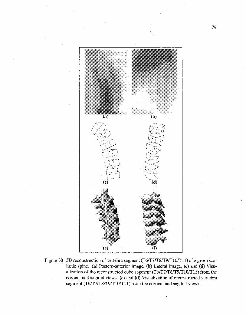
Reproduced with permission of the copyright owner. Further reproduction prohibited without permission.
79
(b)
(e) (f)
Figure 30 3D reconstruction of vertebra segment (T6ff7/T8ff9/T10/Tll) of a given scoliotic spine. (a) Postero-anterior image, (b) Lateral image, (c) and (d) Visualization of the reconstructed cube segment (T6/T7/T8/T9/T10/Tll) from the coronal and sagittal views. (c) and (d) Visualization of reconstructed vertebra segment (T6ff7/T8ff9/Tl0/Tll) from the coronal and sagittal views
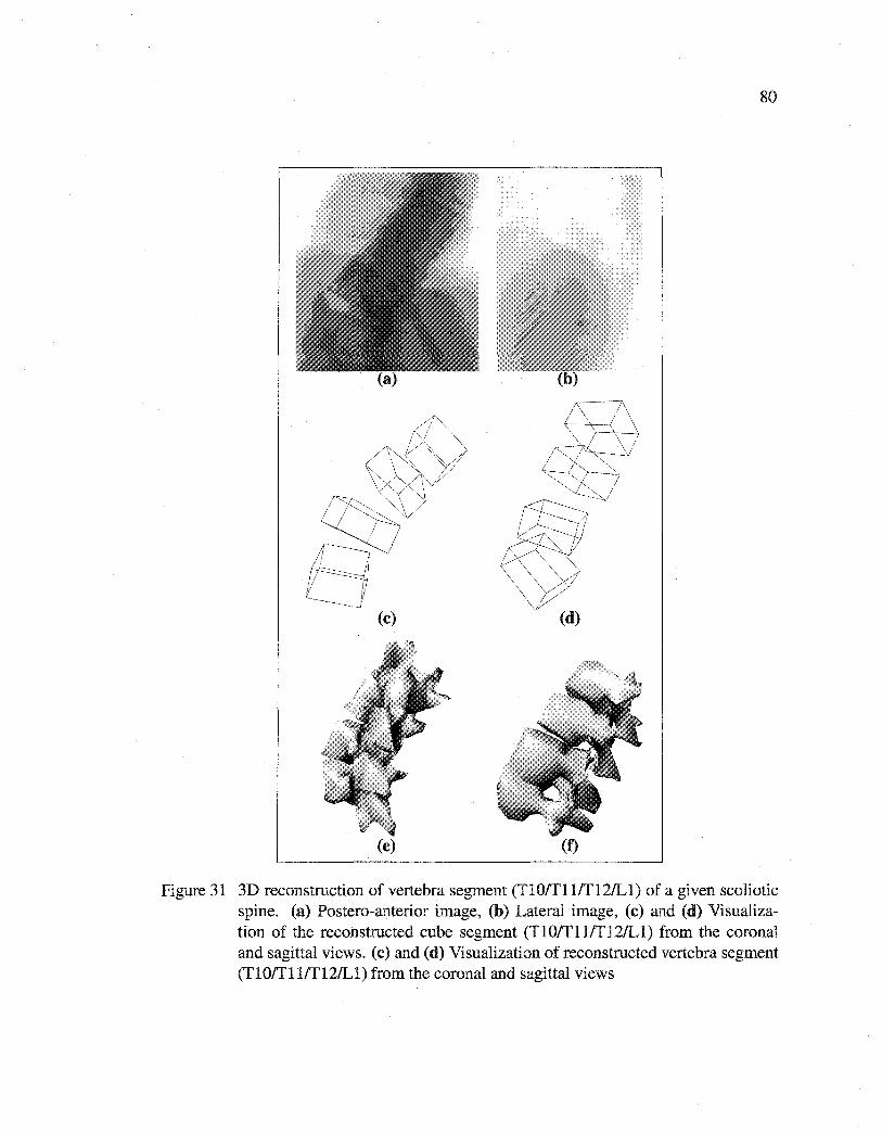
Reproduced with permission of the copyright owner. Further reproduction prohibited without permission.
80
(c)
(e) (f)
Figure 31 3D reconstruction of vertebra segment (Tl0ffll/Tl2/Ll) of a given scoliotic spine. (a) Postero-anterior image, (b) Lateral image, (c) and (d) Visualization of the reconstructed cube segment (Tl0/Tllffl2/Ll) from the corona! and sagittal views. (c) and (d) Visualization of reconstructed vertebra segment (Tl0ffllff12/Ll) from the coronal and sagittal views
Reproduced with permission of the copyright owner. Further reproduction prohibited without permission.
81
This optimization procedure is fast compared to other minimization techniques such as the
gradient-based method and genetic algorithm. This method has been tested on a number
of pairs of radiographie images demonstrating its efficiency and robustness.
The mean error is (1.45 ± 1.46)mm for lumbar vertebra and (1.27 ± 1.29)mm for thoracic
vertebra. The maximumerroris (5.35±0.93)mmfor lumbarvertebra and (4.53±0.82)mm
for thoracic vertebra for our 3D reconstruction technique.
The proposed scheme thus constitutes an alternative to CT-scan 3D reconstruction with
the advantage of low irradiation and will be of great interest for evaluation of spinal defor
mities, simulation of orthopaedic treatments, and for reliable geometrie models for finite
element studies. However, this reconstruction method is not suitable without improve
ment for surgical navigation applications when compared to CT-scan reconstruction errors
of ±lmm, the gold standard for those applications.
The proposed method remains sufficiently general to be applied to other medical recon
struction problems (i.e., rib cage, pelvis, knee, etc.) for which a database of the anatomical
structure is available (with two or more radiographie views).
Reproduced with permission of the copyright owner. Further reproduction prohibited without permission.
RECONSTRUCTION 3D BIPLANAIRE NON SUPERVISÉE DE LA CAGE THORACIQUE SCOLIOTIQUE PAR
UN MÉLANGE DE MODÈLES A PRIORI PROBABILISTES
82
Article : Unsupervised 3D biplanar reconstruction of scoliotic rib cage using the es
timation of a mixture of probabilistic prior models
Cet article a été soumis au journal IEEE Transactions on Biomedical Engineering comme
l'indique la référence bibliographique
S. Benameur, M. Mignotte, F. Destrempes and J.A. De Guise. Unsupervised 3D biplanar
reconstruction of scoliotic rib cage using the estimation of a mixture of probabilistic prior
models. IEEE Transactions on Biomedical Engineering, soumis, 2004.
Cet article est présenté ici dans sa version originale.
Résumé
La cage thoracique protège et supporte les organes internes du corps humain. Elle per
met aussi la mobilité du tronc lors des mouvements d'inspiration et d'expiration. Les dé
formations de la cage thoracique sont des conséquences importantes de la scoliose. La
reconstruction 3D de la cage thoracique scoliotique à partir d'un ensemble d'images ra
diographiques n'a pas souvent été étudiée dans la littérature et peu de références existent à
ce jour [24][77]. Nous présentons dans cet article une méthode originale et non supervisée
de reconstruction 3D des cages thoraciques scoliotiques à partir de deux images radiogra
phiques conventionnelles (postéro-antérieure avec incidence de oo et latérale) calibrées.
Dans la méthode présentée, nous avons supposé que chacune des formes des cages tho
raciques est distribuée dans une classe de pathologie scoliotique spécifique, pour laquelle
nous avons ensuite défini une réduction de dimensionnalité linéaire d' ACP probabiliste.
Dans ce contexte nous avons utilisé un mélange d' ACP probabiliste dont chaque com
posante représente une classe de déformation particulière de la scoliose. Pour chacune
Reproduced with permission of the copyright owner. Further reproduction prohibited without permission.
83
de ces composantes, un modèle a priori paramétrique de forme tridimensionnelle est uti
lisé pour contraindre notre problème mal-posé de reconstruction 3D. La reconstruction
de la cage thoracique relative à chacune des composantes consiste à ajuster les projec
tions (postéro-antérieure et latérale) du modèle a priori 3D de la cage thoracique avec
les contours préalablement segmentés sur les deux images radiographiques calibrées. Le
problème de reconstruction 3D est vu comme un problème d'estimation des paramètres
de déformation de ce modèle ou, de façon équivalente, comme un problème de minimi
sation d'une fonction d'énergie. Cette minimisation est effectuée à l'aide d'un algorithme
stochastique d'exploration/sélection [79]. Les paramètres du mélange d' ACP probabiliste
sont estimés par une version stochastique de l'algorithme EM (Expectation, Maximiza
tion) appelée SEM [33]. La reconstruction 3D optimale correspond à la composante de la
déformation et aux paramètres menant à 1' énergie minimale. La méthode proposée a été
validée sur un échantillon d'une vingtaine de paires d'images radiographiques calibrées
n'appartenant pas à la base d'apprentissage et comparée aux reconstructions 3D issues de
la méthode stéréo-radiographique [24]. Une erreur moyenne de (1.62 ± 0.50) mm a été
obtenue sur les distances point-surface entre le modèle reconstruit avec notre méthode et le
modèle issu de la reconstruction stéréo-radiographique [24]. La reconstruction 3D d'une
cage thoracique scoliotique nécessite un temps de calcul de l'ordre de 6 minutes (sur un
PC/Linux à 2.0 GHz).
Reproduced with permission of the copyright owner. Further reproduction prohibited without permission.
CHAPITRES
UNSUPERVISED 3D BIPLANAR RECONSTRUCTION OF SCOLIOTIC RIB CAGE USING THE ESTIMATION OF A MIXTURE
OF PROBABILISTIC PRIOR MODELS
Abstract In this paper, we present an original method for the automatic 3D reconstruction of the scoliotic rib cage from a planar and a conventional pair of calibrated radiographie
images (postero-anterior with normal incidence and lateral). To this end, we fust present
a robust method for estimating the model parameters in a mixture of Probabilistic Prin
cipal Component Analysers (PPCA). This method is based on the Stochastic Expectation
Maximization (SEM) algorithm. Parameters of this mixture model are used to constrain
the 3D biplanar reconstruction problem of scoliotic rib cage. More precisely, the pro
posed PPCA mixture model is exploited for dimensionality reduction and to obtain a set
of probabilistic prior models associated with each detected class of pathological defor
mations observed on a representative training scoliotic rib cage population. By using an
appropriate likelihood, for each considered class-conditional prior model, the proposed
3D reconstruction is stated as an energy function minimization problem, which is solved
with an exploration/selection algorithm. The optimal 3D reconstruction then corresponds
to the class of deformation and parameters leading to the minimal energy. This 3D method
of reconstruction has been successfully tested and validated on a database of 20 pairs of
biplanar radiographie images of scoliotic patients, yielding very promising results. As an
alternative to CT-scan 3D reconstruction this scheme has the advantage of low radiation
for the patient, and may also be used for diagnosis and evaluation of deformity of a sco
liotic rib cage. The proposed method remains sufficiently general to be applied to other
reconstruction problems for which a database of objects to be reconstructed is available
(with two or more radiographie views).
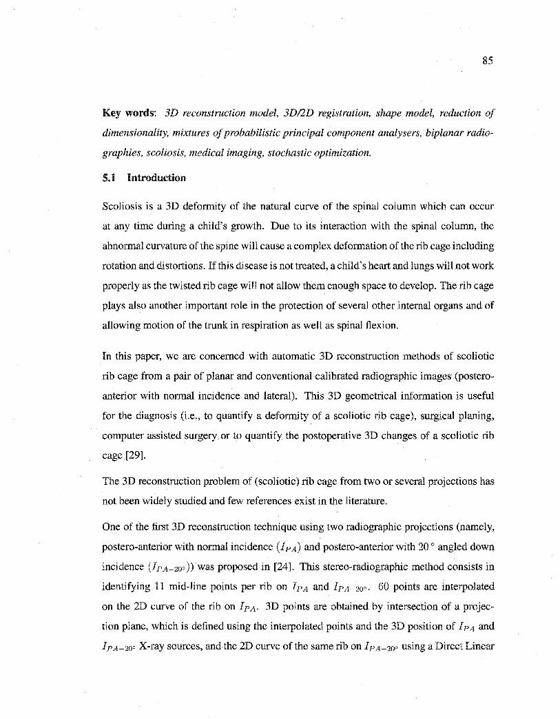
Reproduced with permission of the copyright owner. Further reproduction prohibited without permission.
85
Key words: 3D reconstruction madel, 3D/2D registration, shape madel, reduction of
dimensionality, mixtures of probabilistic principal component analysers, biplanar radio
graphies, scoliosis, medical imaging, stochastic optimization.
5.1 Introduction
Scoliosis is a 3D deformity of the natural curve of the spinal column which can occur
at any time during a child's growth. Due toits interaction with the spinal column, the
abnormal curvature of the spine will cause a complex deformation of the rib cage including
rotation and distortions. If this disease is not treated, a child's heart and lungs will not work
properly as the twisted rib cage will not allow them enough space to develop. The rib cage
plays also another important role in the protection of several other internai organs and of
allowing motion of the trunk in respiration as well as spinal flexion.
In this paper, we are concemed with automatic 3D reconstruction methods of scoliotic
rib cage from a pair of planar and conventional calibrated radiographie images (postero
anterior with normal incidence and lateral). This 3D geometrical information is useful
for the diagnosis (i.e., to quantify a deformity of a scoliotic rib cage), surgical planing,
computer assisted surgery or to quantify the postoperative 3D changes of a scoliotic rib
cage [29].
The 3D reconstruction problem of (scoliotic) rib cage from two or several projections has
not been widely studied and few references exist in the literature.
One of the first 3D reconstruction technique using two radiographie projections (namely,
postero-anterior with normal incidence ( 1 pA) and postero-anterior with 20 o angled down
incidence (IPA- 2oo )) was proposed in [24]. This stereo-radiographie method consists in
identifying 11 mid-line points per rib on ]pA and IPA-2oo. 60 points are interpolated
on the 2D curve of the rib on !PA· 3D points are obtained by intersection of a projec
tion plane, which is defined using the interpolated points and the 3D position of !PA and
I pA_ 20o X-ray sources, and the 2D curve of the same rib on 1 pA_ 20o using a Direct Linear
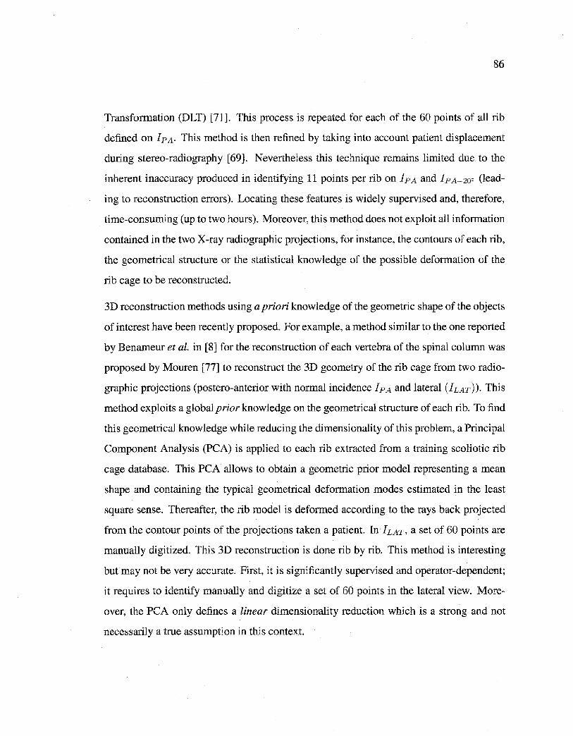
Reproduced with permission of the copyright owner. Further reproduction prohibited without permission.
86
Transformation (DLT) [71]. This process is repeated for each of the 60 points of all rib
defined on I pA. This method is then refined by taking into account patient displacement
during stereo-radiography [69]. Nevertheless this technique remains limited due to the
inherent inaccuracy produced in identifying 11 points per rib on !PA and IPA-2oo (lead
ing to reconstruction errors). Locating these features is widely supervised and, therefore,
time-consuming (up to two hours). Moreover, this method does not exploit all information
contained in the two X-ray radiographie projections, for instance, the contours of each rib,
the geometrical structure or the statistical knowledge of the possible deformation of the
rib cage to be reconstructed.
3D reconstruction methods using a priori knowledge of the geometrie shape of the abjects
of interest have been recently proposed. For example, a method similar to the one reported
by Benameur et al. in [8] for the reconstruction of each vertebra of the spinal column was
proposed by Mouren [77] to reconstruct the 3D geometry of the rib cage from two radio
graphie projections (postero-anterior with normal incidence I pA and lateral (hAT)). This
method exploits a global prior knowledge on the geometrical structure of each rib. To find
this geometrical knowledge while reducing the dimensionality of this problem, a Principal
Component Analysis (PCA) is applied to each rib extracted from a training scoliotic rib
cage database. This PCA allows to obtain a geometrie prior model representing a mean
shape and containing the typical geometrical deformation modes estimated in the least
square sense. Thereafter, the rib model is deformed according to the rays back projected
from the contour points of the projections taken a patient. In hAT· a set of 60 points are
manually digitized. This 3D reconstruction is done rib by rib. This method is interesting
but may not be very accurate. First, it is significantly supervised and operator-dependent;
it requires to identify manually and digitize a set of 60 points in the lateral view. More
over, the PCA only defines a linear dimensionality reduction which is a strong and not
necessarily a true assumption in this context.
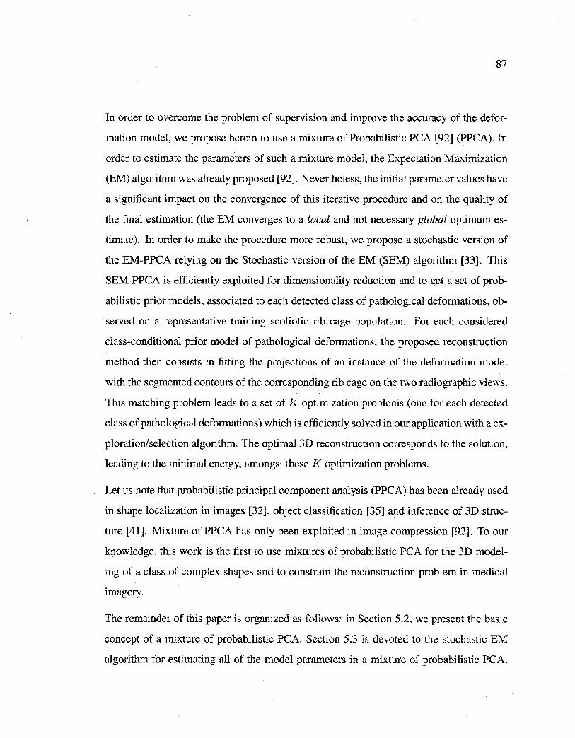
Reproduced with permission of the copyright owner. Further reproduction prohibited without permission.
87
In order to overcome the problem of supervision and improve the accuracy of the defor
mation model, we propose herein to use a mixture of Probabilistic PCA [92] (PPCA). In
order to estimate the parameters of such a mixture model, the Expectation Maximization
(EM) algorithm was already proposed [92]. Nevertheless, the initial parameter values have
a significant impact on the convergence of this iterative procedure and on the quality of
the final estimation (the EM converges to a local and not necessary global optimum es
timate ). In order to make the procedure more robust, we propose a stochastic version of
the EM-PPCA relying on the Stochastic version of the EM (SEM) algorithm [33]. This
SEM-PPCA is efficiently exploited for dimensionality reduction and to get a set of prob
abilistic prior models, associated to each detected class of pathological deformations, ob
served on a representative training scoliotic rib cage population. For each considered
class-conditional prior model of pathological deformations, the proposed reconstruction
method then consists in fitting the projections of an instance of the deformation model
with the segmented contours of the corresponding rib cage on the two radiographie views.
This matching problem leads to a set of K optimization problems (one for each detected
class of pathological deformations) which is efficiently solved in our application with a ex
ploration/selection algorithm. The optimal 3D reconstruction corresponds to the solution,
leading to the minimal energy, amongst these K optimization problems.
Let us note that probabilistic principal component analysis (PPCA) has been already used
in shape localization in images [32], object classification [35] and inference of 3D struc
ture [41]. Mixture of PPCA has only been exploited in image compression [92]. To our
knowledge, this work is the first to use mixtures of probabilistic PCA for the 3D model
ing of a class of complex shapes and to constrain the reconstruction problem in medical
imagery.
The remainder of this paper is organized as follows: in Section 5.2, we present the basic
concept of a mixture of probabilistic PCA. Section 5.3 is devoted to the stochastic EM
algorithm for estimating all of the model parameters in a mixture of probabilistic PCA.
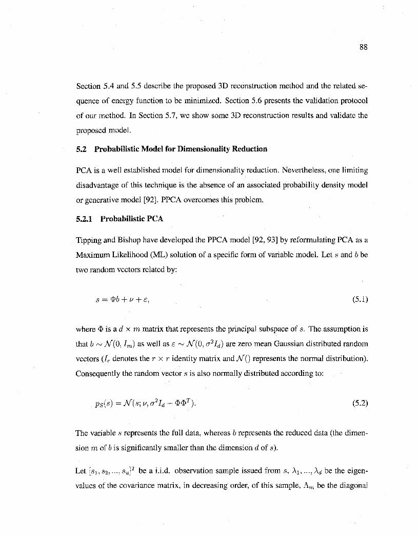
Reproduced with permission of the copyright owner. Further reproduction prohibited without permission.
88
Section 5.4 and 5.5 describe the proposed 3D reconstruction method and the related se
quence of energy function to be minimized. Section 5.6 presents the validation protocol
of our method. In Section 5.7, we show sorne 3D reconstruction results and validate the
proposed model.
5.2 Probabilistic Model for Dimensionality Reduction
PCA is a weil established model for dimensionality reduction. Nevertheless, one lirniting
disadvantage of this technique is the absence of an associated probability density model
or generative model [92]. PPCA overcomes this problem.
5.2.1 Probabilistic PCA
Tipping and Bishop have developed the PPCA model [92, 93] by reformulating PCA as a
Maximum Likelihood (ML) solution of a specifie form of variable model. Let s and b be
two random vectors related by:
(5.1)
where <I> is a d x m matrix that represents the principal subspace of s. The assumption is
that b rv N(O, lm) as well as E rv N(O, Œ2 Id) are zero mean Gaussian distributed random
vectors Ur denotes the r x r identity matrix and N() represents the normal distribution).
Consequently the random vector s is also normally distributed according to:
(5.2)
The variables represents the full data, whereas b represents the reduced data (the dimen
sion m of b is significantly smaller than the dimension d of s ).
Let [s1 , s2, ... , suJT be a i.i.d. observation sample issued from s, .\1 , ... , Àd be the eigen
values of the covariance matrix, in decreasing order, of this sample, Am be the diagonal
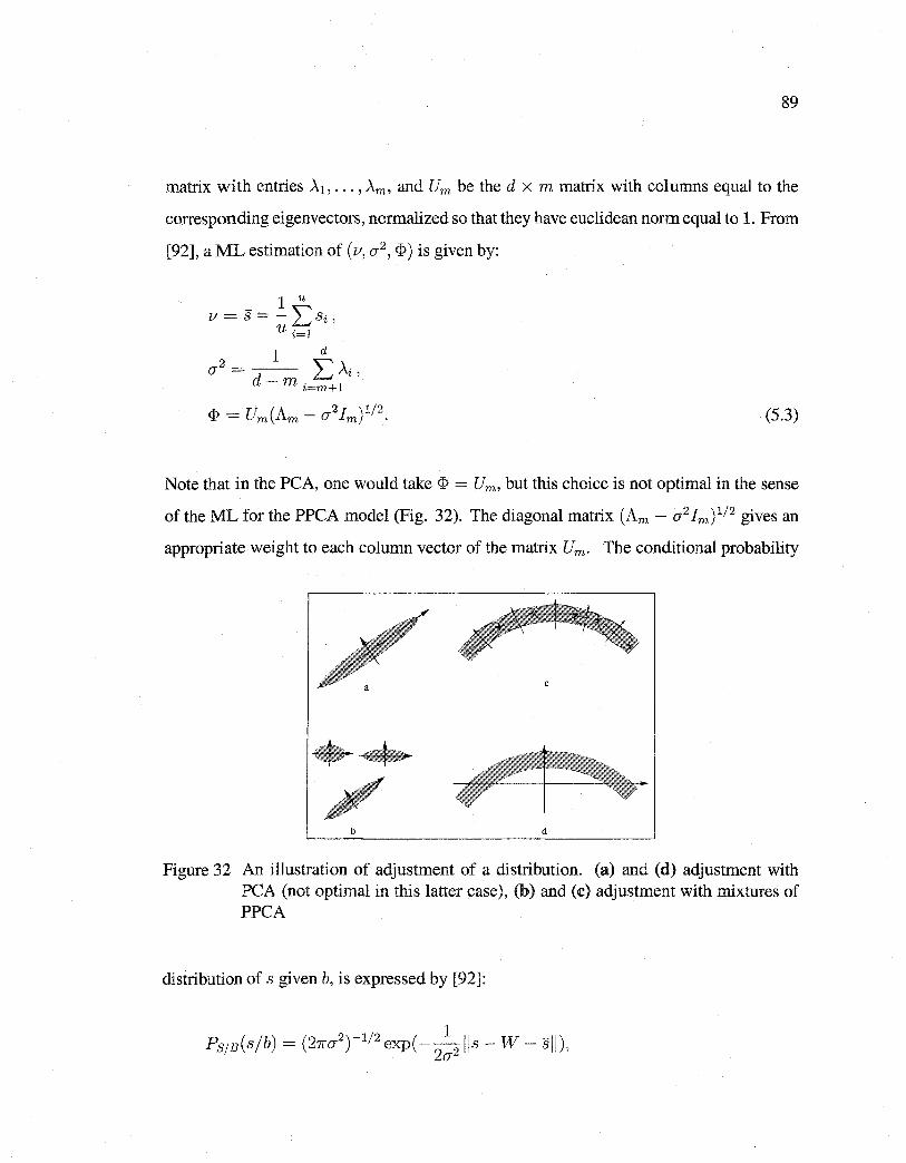
Reproduced with permission of the copyright owner. Further reproduction prohibited without permission.
89
matrix with entries À1, ... , Àm, and Um be the d x m matrix with columns equal to the
corresponding eigenvectors, normalized so that they have euclidean norm equal to 1. From
[92], a ML estimation of (v, o-2 , <I>) is given by:
1 u v= s=- l:si,
u i=l
1 d
o-2 = d- 1:.: Ài, m i=m+l
(5.3)
Note that in the PCA, one would take <I> = Um, but this choice is not optimal in the sense
of the ML for the PPCA model (Fig. 32). The diagonal matrix (Am - o-2 Im) 112 gives an
appropriate weight to each column vector of the matrix Um. The conditional probability
c
•• b d
Figure 32 An illustration of adjustment of a distribution. (a) and (d) adjustment with PCA (not optimal in this latter case), (b) and (c) adjustment with mixtures of PPCA
distribution of s given b, is expressed by [92]:
1 Ps;s(sjb) = (21ro-2
)-112 exp( --
2JJs- W- sJJ),
2o-
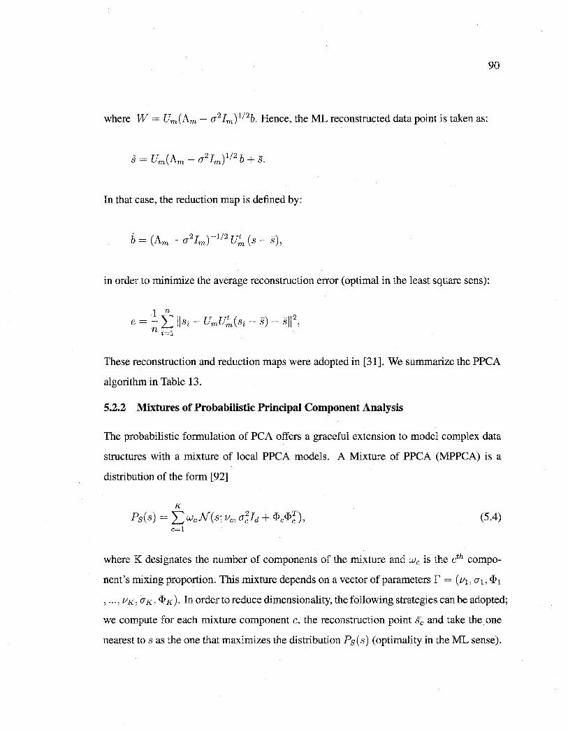
Reproduced with permission of the copyright owner. Further reproduction prohibited without permission.
90
where W = Um(Am- CJ2 Im) 112 b. Hence, the ML reconstructed data pointis taken as:
In that case, the reduction map is defined by:
in order to minimize the average reconstruction error (optimal in the !east square sens):
These reconstruction and reduction maps were adopted in [31]. We summarize the PPCA
algorithm in Table 13.
5.2.2 Mixtures of Probabilistic Principal Component Analysis
The probabilistic formulation of PCA offers a graceful extension to model complex data
structures with a mixture of local PPCA models. A Mixture of PPCA (MPPCA) is a
distribution of the form [92]
K
Ps(s) = l:wcN(s; Vc, CJ~!d + ~c~~), (5.4) c=l
where K designates the number of components of the mixture and wc is the eth compo
nent's mixing proportion. This mixture depends on a vector of parameters r = (v1 , CJ1 , ~1
, ... , vK, CJK, ~K ). In ordertoreduce dimensionality, the following strategies can be adopted;
we compute for each mixture component c, the reconstruction point sc and take the one
nearest to sas the one that maximizes the distribution P8 (s) (optimality in the ML sense).
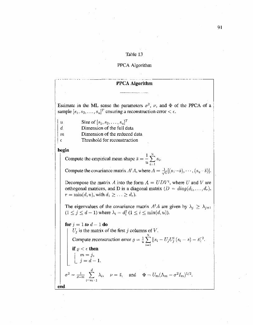
Reproduced with permission of the copyright owner. Further reproduction prohibited without permission.
Table 13
PPCA Algorithm
PPCA Algorithm
Estimate in the ML sense the parameters cr2, v, and <I> of the PPCA of a
sample [s1, s2 , ... , suJT ensuring a reconstruction error < E.
u Size of [s1 , s2 , ... , su]T d Dimension of the full data m Dimension of the reduced data E Threshold for reconstruction
begin
Compute the empirical mean shape s = _!. t si. u i=l
Compute the covariancematrix At A, where A= ju[(s1-s), ···,(su-s)].
Decompose the matrix A into the form A = U DVt, where U and V are orthogonal matrices, and Dis a diagonal matrix (D = diag(d1 , ... , dr), r = min(d, u), with d1 ~ ... ~dr).
The eigenvalues of the covariance matrix At A are given by Àj > Àj+l
(1 :::; j :::; d- 1) where >..i =dr (1 :::; i :::; min(d, u)).
for j = 1 to d - 1 do uj is the matrix of the first j columns of v.
u
Compute reconstruction error f2 = ~ L llsi- UjUJ (si - s)- sll 2•
i=l if f2 < E then
l m=J, j=d-1.
d 2_ 1 """ \
CT - d-m L..t Ai' 1/ = s, i=m+l
end
91
Reproduced with permission of the copyright owner. Further reproduction prohibited without permission.
92
5.3 Estimation of a Mixture of PPCA
In order to estimate parameter vector r, we resort to the SEM algorithm [33]. This iter
ative procedure requires initial parameters which can be given by a K -means clustering
procedure [ 45] (in doing so, we assume as fust approximation that the considered clus
ters are spherical with equal volumes). The obtained spherical partitions allow to obtain
a rough estimation of the mixture parameters which are then used to initialize the SEM
clustering and estimation procedure.
5.3.1 K -means Algorithm
The K -means algorithm consists of the following steps. To initialize K clusters, choose
K shapes at random from the training base. For each shape selected in the training base,
assign this shape to a class such that the Euclidean distance from this shape to the center
of that cluster is minimal. For each cluster, recalculate the means of the cluster based on
the shapes that belong to that cluster. This second step is running until the center of each
class becomes steady.
5.3.2 Stochastic EM Algorithm
Let K be an upper bound on the number of classes and Ç E] 0, 1 [ be a chosen threshold. In
the context of the estimation of a MPPCA, the SEM algorithm can be outlined as follows,
(the superscript denoting the iteration number).
Initialization
We initialize the SEM algorithm by the ML parameters estimated on the complete data
obtained by a K-means [45] partition of [s1 , s2 , ... , suf into K classes. For every obser
vation si, the probability P~~lc(sï/c) of its belonging to the class c, (cE {1, ... , K}) can
then be defined. This terminates the initialization phase.
An iteration of SEM then consists of three steps.
Reproduced with permission of the copyright owner. Further reproduction prohibited without permission.
93
Step S (Stochastic)
For each si, we select from the set of classes an element according to the distributions
[PJf)s(1/ Si, r(pl), 0 0 0 'PJf)s(K/ Si, r(pl)]o This selection defines a partition [19rl' 0 0 0 '19WJ
of the sample [s1, s2, ooo' sufo
Step M (Maximization)
The SEM algorithm supposes that every si belonging to '!9Jfl for each c E [1, K], is real
ized according to the distribution defined by P810 ( sd c, r) (Eq. (5.2)), the density cor
responding to class c. Let u be the number of rib cages in the training base. The pa
rameters of the mixture are estimated for the complete data in the ML sense upon setting
7r!f+Il = Card(19Jrl)ju and estimating r(p+I] on each class according to (Eq. (5.3)). If
?fJf+Il < Ç, we eliminate the class c in the mixture.
Step E (Estimation)
For each Si' we define the next distribution [pc 1 s ( 11 si' r(p+I]) ' 0 0 0 ' pc 1 s ( K 1 Si' r(p+I]) l by the posterior distribution based on the current parameter r(p+I] :
[p+l]p ( 1 flP+ll) n ( j . f[p+l]) - 1re SIC Si C, rc1s c s%, - K [p+I] .
I:e=l 1re P810 (sï/c, flP+ll)
Retum to step S until the maximum number of iterations has been reached.
5.4 Mixture of Statistical Deformable Models
The shape s of each rib cage of our training database is defined by a set of l control points,
or landmarks, which approximate the geometrical shape of the mid-line of each rib in R}.
Bach rib cage in the training set is thus represented by the following 3l dimensional vector,
s = (xl, Y1, z1, ... , Xz, Yz, zz)t,
Reproduced with permission of the copyright owner. Further reproduction prohibited without permission.
94
where (xi, Yi, zi) t are the Cartesian coordinates of the ith control point or landmark of the
shape.
5.4.1 Training phase
First, we extend into 3D the method proposed by Cootes in [17] for aligning the set of
u 3D shape samples [s1 , s2 , ... ,su] of our training database to a common scale, rotation,
and translation. This step is important and allows to eliminate the variations introduced
by affine deformations such as translation, scaling, and rotation.
To this end, an arbitrary shape is selected as the initial average shape estimate. Ali the
other shapes are aligned to this average using a least square minimization. A new average
is computed by a simple mean across the corresponding points, and the procedure repeats
until convergence. Assuming that 3D translation is represented by a separate translation
vector t, a quaternion3 q representation of scaling and rotation avoids such behavior [51].
Thus, any scaling and rotation in 3D can be expressed as quaternion, where scaling is
expressed by the magnitude of the quaternion and the 3D rotation is expressed by the
direction of the unit vector u and rotation cp. Quaternion have sorne advantages amongst
which simple derivatives and efficient formulations to find rotation matrices directly for
point matching problems [10]. The alignment of two 3D shape instances is accomplished
using a well-known procedure given in [10] to optimize for q and t.
We then apply the MPPCA to estimate the parameters of each class and to reduce the
dimension to mc ~ 3l (Fig. 33). Viewing sc = (x1, y1, z1, ... , Xz, yz, zz) as a random
vector, we obtain, for each class c ( c E [ 1, K]), an optimal probabilistic deformable model
3 A quaternion q is defined as the linear combination of a scalar term q0 ;::: 0 and three right-handed orthonormal vectors (i, j, and k) q = qo + q1i + q2j + q3k. The magnitude of the quaternion is defined as, 1 q 1= Jq5 + qr + q~ + q§, and any unit length quaternion can be written as, q = cos( cp) · u + sin( cp) · u, where u is a unit vector and cp represents a rotational twist along the unit vector. The Cartesian rotation matrix is given by,
2(qlq2- qoq3) q5 + q~ - qr - q§
2(q2q3 + qoq1)
Reproduced with permission of the copyright owner. Further reproduction prohibited without permission.
95
in the ML sense of the form Sc= <I>cbc+vc+Ec with Ec rv N(O, O"~lz), IÎ>c a 3l X mc matrix,
and be t'V N(O, ImJ, by taking Vc = Sc, (}"~ = 1-lmc L:~=mc+l Ài, and <I>c = UmJAmc -
O"~lmJ 1 1 2 • This gives us non-linear deformations of the mean shape of each pathological
deformations detected in our representative learning set, and terminates the training phase
(Figs. 34 and 35).
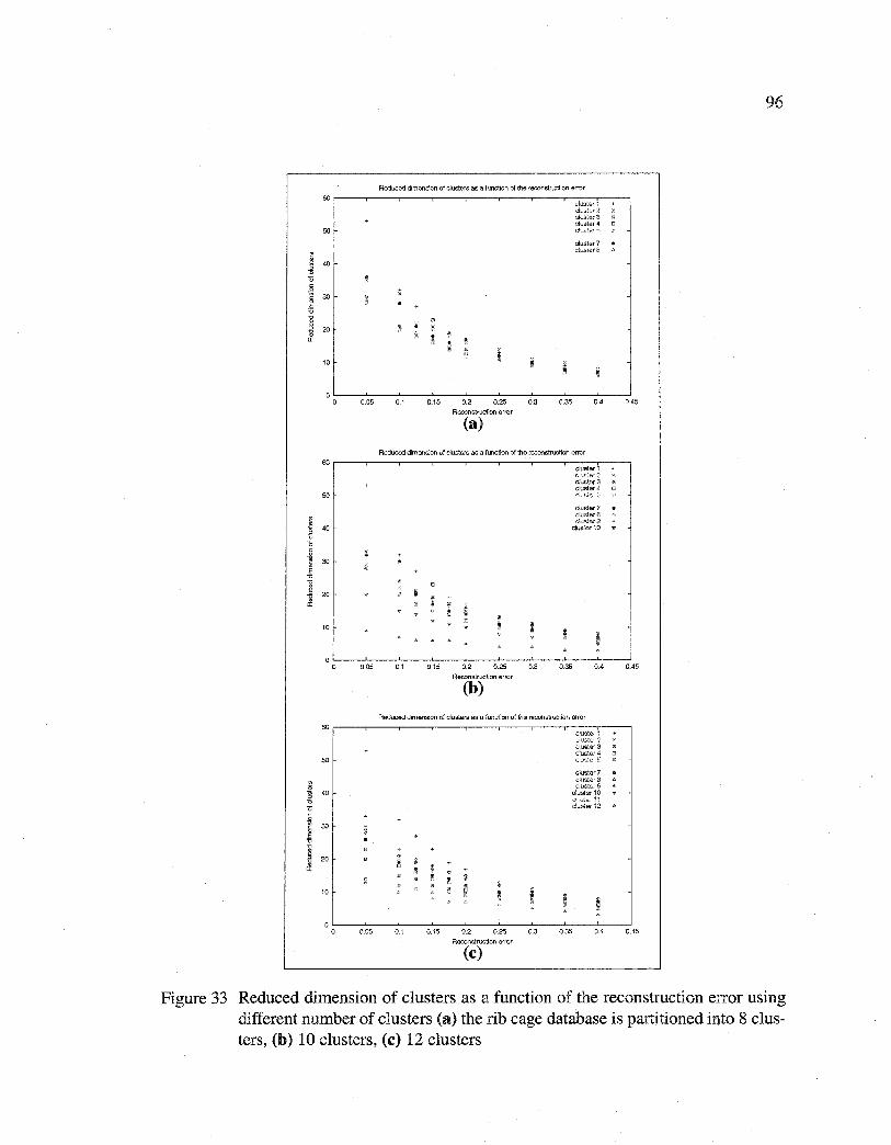
Reproduced with permission of the copyright owner. Further reproduction prohibited without permission.
60
50
i 40
" 0
1 30
~
l 20
a:
10
0 0 0.05
60
50
1 40
" 0
i 30
~ @
20
" cr:
10
0 0 0.05
60
50
j 4()
" 0 .Q
J 30
~ 20
" cr:
10
0 0 0.05
Reduced dimension of c!usters as a function of the reconstruction error
01 0.15 0.2 0.25
Reconstruction error
(a)
0.3 0.35
cluster7 ciuswr.S
0.4
Reducad dimension of c\ustars as a funclion of the reconstruction errer
01 015 0.2 0.25
Reconstruction error
(b)
0.3
cluster i L·l:&',-?lr2 c!uster3 clustar4 dl'·'·:·:,
clustar7 c!uste-rB clt..s~er 9
cluster10
0.35 0.4
Aeduced dimension of clusters as a function of the reconstruction error
c!ustar7 ciuster8 -:;luster5
oluster 10 .:;li,~Ls- ·ir c!uS.er 12
0.1 0.15 0.2 0.25 0.3 035 04
Raconstruction error
(c)
96
045
0.45
0.45
Figure 33 Reduced dimension of clusters as a function of the reconstruction error using different number of clusters (a) the rib cage database is partitioned into 8 clusters, (b) 10 clusters, (c) 12 clusters
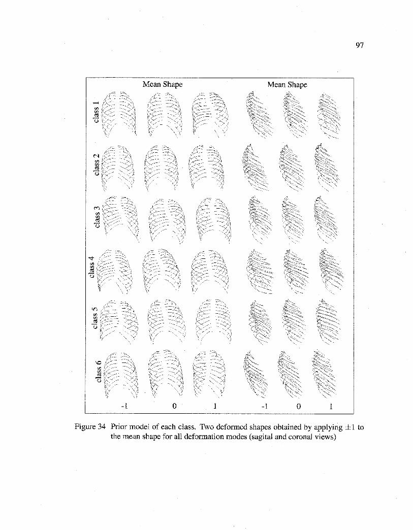
Reproduced with permission of the copyright owner. Further reproduction prohibited without permission.
97
Mean Shape Mean Shape
-1 0 1 -1 0 1
Figure 34 Prior model of each class. Two deformed shapes obtained by applying ±1 to the mean shape for all deformation modes (sagital and coronal views)
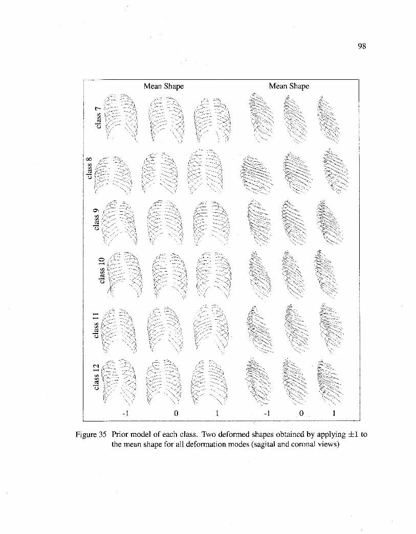
Reproduced with permission of the copyright owner. Further reproduction prohibited without permission.
00 Cil
~ -u
Mean Shape
-1 0
98
Mean Shape
1 -1 0 1
Figure 35 Prior model of each class. Two deformed shapes obtained by applying ±1 to the mean shape for all deformation modes (sagital and coronal views)
Reproduced with permission of the copyright owner. Further reproduction prohibited without permission.
99
5.4.2 Deformation parameters
From the training phase, we obtain for each class c ( c E [1, K]), the mean shape sc, and its
non-lineardeformations Sc= <Pc be+ Sc, where <Pc= [U1(A1- aiJI)112, ... , Umc(Amc
a~ImJ 112 ] is the matrix of the first mc eigenvectors associated with the mc largest eigenval
ues and he= (bc,l, ... , bc,mJt is a vector containing the weights for these mc deformation
modes.
In addition, we consider rigid deformations of the template given by global translation
T = (tx, ty, tz), scaling k = (kx, ky, kz), and rotation a = (ax, ay, az) around the x, y
and z, axis (applied point-wise to the template). This yields a vector of deformation:
e = (T, k, a, be),
of dimension 9 + mc. The globally deformed template for class c is then defined by:
(5.5)
where M(k, a) performs a rotation and a scaling by k.
5.4.3 Prior energy term
Let 8c be the random variable corresponding to the vector of (9 +mc) deformations. We
model the distribution of 8c by [32],
(5.6)
where U is the uniform distribution. This probability expresses the fact that the shape to
be reconstructed is likely close to the mean shape. By considering that,
Reproduced with permission of the copyright owner. Further reproduction prohibited without permission.
100
(5.7)
where (p is a normalization constant, a prior energy term can be deduced from this low
parametric representation,
(5.8)
This energy term, which does not penalize affine transformations, will be used in our
energy-based model to rightly constrain our 3D reconstruction model by penalizing the
deviation of the deformed template from the mean shape.
5.4.4 Likelihood energy term
In a commonly used energy-based (deformable) model of reconstruction or segmentation,
spatial contours (or sorne spatial gradient measures derived from the input image) are
generally exploited in the data likelihood energy term. This term aims at expressing a
measure of similarity between the deformed template and the object present in the image
by constraining the deformable template to be attracted and aligned to the salient edges
of the object to be detected [8]. Due to the low signal-to-noise ratio, low resolution and
contrast of the radiographie images used in our application, the sharpness of the contour
of each rib is noticeably reduced and our likelihood model cannot rely efficient! y solely on
this type of gradient measures. Instead, we propose a likelihood energy term exploiting an
edge potential field [8] along with a statistical region-based homogeneity criterion. This
measure is based on the computation of the grey-level variance inside and outside each
rib. In our application, the likelihood energy term is expressed as,
(5.9)
where E1(sc(B), IPA) and Ez(sc(B), fLAT) are likelihood energy terms for postero-anterior
and lateral images respective! y, with, for the postero-anterior image,
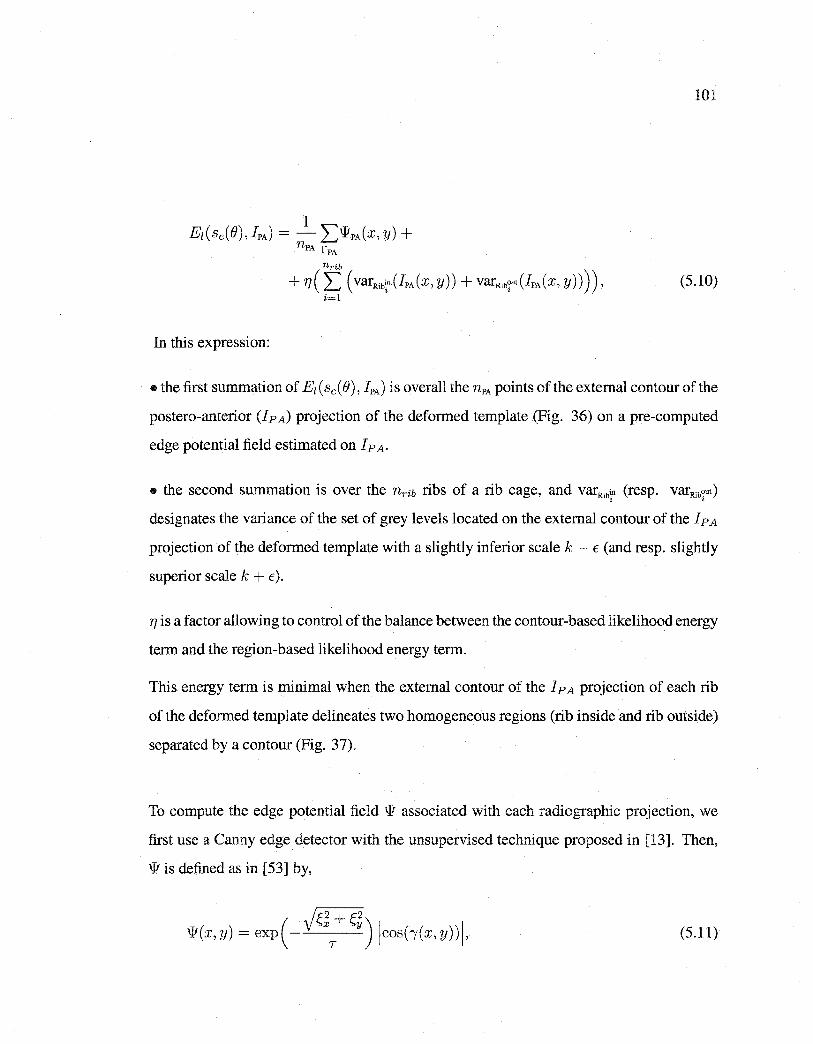
Reproduced with permission of the copyright owner. Further reproduction prohibited without permission.
101
1 Ez(sc(e), JPA) =- L:wPA(x, y)+
nPA rPA nrib
+ 11( L ( varRibf(JPA (x, Y)) + varrub1ut(JPA (x, y)))), (5.10) i=l
In this expression:
ethe first summation of Ez (sc( 0), JPA) is overall the nPA points of the extemal contour of the
postero-anterior (IpA) projection of the deformed template (Fig. 36) on a pre-computed
edge potential field estimated on I pA.
e the second summation is over the nrib ribs of a rib cage, and varRibiu (res p. varrubout) ' '
designates the variance of the set of grey levels located on the extemal contour of the I pA
projection of the deformed template with a slightly inferior scale k - E (and resp. slightly
superior scale k + E).
17 is a factor allowing to control of the balance between the contour-based likelihood energy
term and the region-based likelihood energy term.
This energy term is minimal when the extemal contour of the !PA projection of each rib
of the deformed template delineates two homogeneous regions (rib inside and rib outside)
separated by a contour (Fig. 37).
To compute the edge potential field w associated with each radiographie projection, we
first use a Canny edge detector with the unsupervised technique proposed in [13]. Then,
w is defined as in [53] by,
je +f} W(X, y)= exp(- XT y) jcos(1(x, y))j, (5.11)
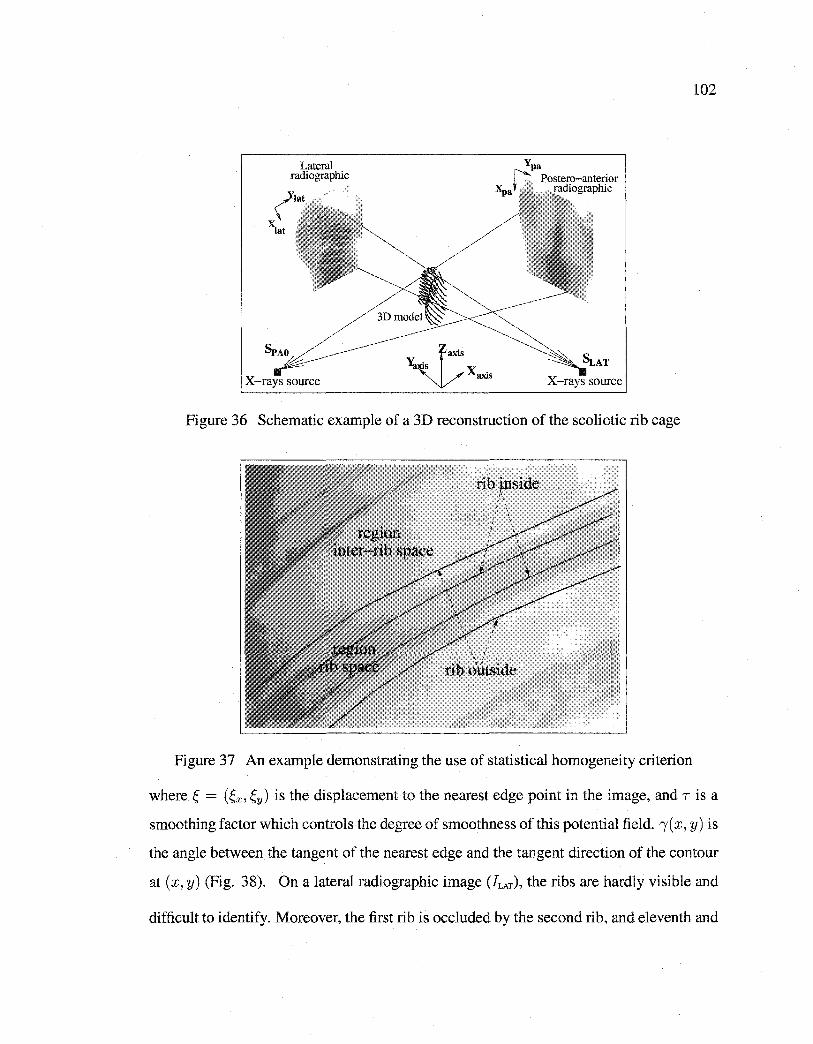
Reproduced with permission of the copyright owner. Further reproduction prohibited without permission.
Lateral radiographie
X-rays source x.
3XIS X-rays source
Figure 36 Schematic example of a 3D reconstruction of the scoliotic rib cage
rib ~nside '•
' '
: \ ' ' J \
rib ~'iitside
Figure 37 An example demonstrating the use of statistical homogeneity criterion
102
where Ç = (Çx, f,y) is the displacement to the nearest edge point in the image, and Tisa
smoothing factor which controls the degree of smoothness of this potential field. 1( x, y) is
the angle between the tangent of the nearest edge and the tangent direction of the contour
at (x, y) (Fig. 38). On a lateral radiographie image (JLAT), the ribs are hardly visible and
difficult to identify. Moreover, the first rib is occluded by the second rib, and eleventh and
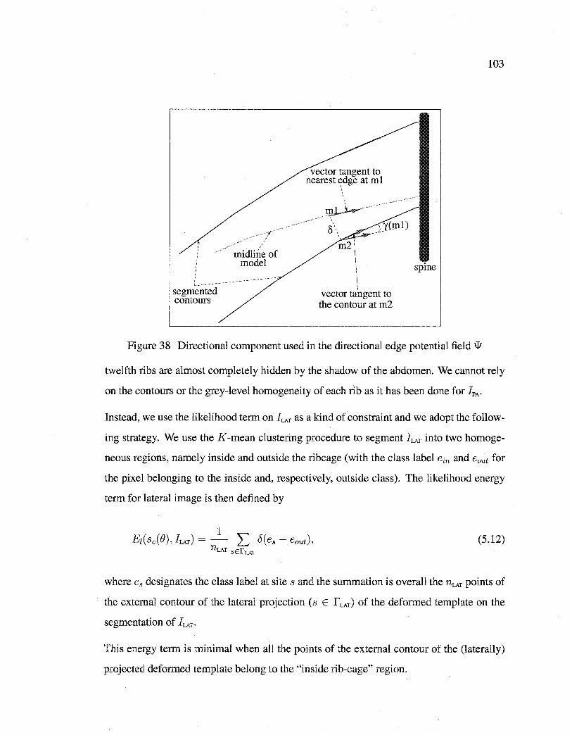
Reproduced with permission of the copyright owner. Further reproduction prohibited without permission.
' ' ' ' ' ' ' ' ' ' ' 1...----segrnented contours
rnidline of rnodel
vector tangent to nearest t?dge at ml
/Jn~---·
' S\
rn2 \ 1
\
\ vector tangent to the contour at rn2
103
spine
Figure 38 Directional component used in the directional edge potential field w
twelfth ribs are almost completely hidden by the shadow of the abdomen. We cannot rely
on the contours or the grey-level homogeneity of each rib as it has been done for IPA·
Instead, we use the likelihood term on !LAT as a kind of constraint and we adopt the follow
ing strategy. We use the K-mean clustering procedure to segment !LAT into two homoge
neous regions, namely inside and outside the ribcage (with the class label ein and eout for
the pixel belonging to the inside and, respectively, outside class). The likelihood energy
term for lateral image is then defined by
(5.12)
where e8 designates the class label at site s and the summation is overall the nLAT points of
the extemal contour of the lateral projection (s E r LAT) of the deformed template on the
segmentation of !LAT·
This energy term is minimal when ali the points of the extemal contour of the (laterally)
projected deformed template belong to the "inside rib-cage" region.
Reproduced with permission of the copyright owner. Further reproduction prohibited without permission.
104
5.4.5 3D Reconstruction
The only supervision required by our proposed reconstruction method consists in placing
manually, using a simple graphical interface, a rectangular bounding box including the
whole rib cage for the JLAT and JPAo radiographie images. Using the center of the two rect
angular bounding boxes, we estimate the 3D point coordinates corresponding to these two
projected centers by the Direct Linear Transformation (DLT) [5]. This estimated center is
then considered as the center of the 3D model. We then use the likelihood matching energy
defined in Section 5.4.4 in order to fit the two projections of an instance of the deformable
model with the two corresponding radiographie images. (Fig. 36). This matching prob
lem leads to a set of K optimization problems (one for each detected class of pathological
deformations) which is efficiently solved in our application with an exploration/selection
algorithm (see Section 5.5). The optimal 3D reconstruction corresponds to the solution,
leading to the minimal energy, amongst these K optimization problems, namely,
EaptimaJ(sc(O)) = arg min { arg min E(sc(O) )}. c e
5.5 Optimization strategy
For each considered class-conditional prior mode! of pathological deformations c ( c E
[1, ... , K]), the unsupervised 3D reconstruction procedure is stated as an energy function
minimization problem, namely
(5.13)
where E1 is the likelihood energy term, Ep is the prior energy term (or regularization term)
restricting the deformation of the prior model sc. {3 is a factor allowing to control the
balance between the two energy components and the rigidity of the deformable template.
The energy function to be minimized is a complex function with severa! local extrema
over the deformation parameter space. A global search is usually impossible due to the
Reproduced with permission of the copyright owner. Further reproduction prohibited without permission.
105
size of the configuration space. Instead, we have irnplemented the exploration/selection
algorithm (E/S).
The E/S algorithm belongs to the class of evolutionary algorithms. This class of algorithm
has been successfully applied in diverse areas such as medical imaging [74], localization of
shapes [32][31], non photorealistic rendering [72], and 3D reconstruction of the scoliotic
spine [8].
The E/S algorithm can be summarized as follows (more details are given in [79]). Let
F be a finite discrete subset of the Cartesian product of ç compact intervals [mi, Mi], for
1 ::; i ::; ç, ande = { e1 , ... , en} be a set of n potential solutions randomly chosen. We
define ê as the minimal element ei of e such that E(sc(ej)) > E(sc(ei)), for 1 ::; j < i,
andE( sc( ej)) 2: E( sc( Bi)), for 1 < j ::; n. We considera graph G defined on F called the
exploration graph. The exploration graph is assumed to be non-oriented and connected.
We denote by N (a) the neighborhood of the element a E F in the graph G defined by [31]
{bEF :for sorne j, lbj- ajl ::; r(Mj -mj), bi= ai, i =!= j} where ris a real number in
interval [0,1] called the radius of exploration.
Bach solution of e is regarded as an individual that attempts a random search on the ex
ploration graph [79]. For b E F, we fix a positive distribution ab on N ( b). The exploration
process acts independently on each individual, and consists of choosing a random N ac
cording to the binomial distribution bin( n, p) where n is the size of the population and p
is the probability of exploration. We replace ei by {Ji EN(ei) \{Ô} according to the uni
form distribution, for i::; N otherwise, we change ei by ê. This process is running until a
criterion is met.
5.6 Validation
The validation of the accuracy of our 3D reconstruction method is a difficult task because
a scanned rib cage database is not available.
Reproduced with permission of the copyright owner. Further reproduction prohibited without permission.
106
In our application, our 3D reconstruction technique is validated by visual examination
and also by comparing the reconstructed model obtained by our method and by the model
resulting from the stereo-radiographie reconstruction technique developed in [24]. The
validation procedure consists in fitting the model of our 3D reconstruction method on the
model resulting from the stereo-radiographie technique for the same scoliotic patient using
quaternion method [51].
5. 7 Experimental results
5.7.1 Rib cages database
The training database consists of 532 ( u = 532) scoliotic rib cages. Ali rib cages have the
same number of ribs (11 right ribs and 11 left ribs ). Midline of each rib is composed of 30
points. The 3D coordinates of midline points of each rib cage were recorded in a specifie
order. The positions of the landmarks of ali rib cages within the database are expressed in
the same coordinate system.
The 3D geometry of each rib cage within our database is obtained using the 3D recon
struction technique developed in [24]. The accuracy of this technique was evaluated using
radio-opaque markers. The mean and standard deviation were 1.01 mm and O. 72 mm [24].
5. 7.2 Radiographie images
In our application, we used two radiographie images (i.e., a postero-anterior with normal
incidence and a lateral) acquired with a Fuji FCR 7501S radiographie imaging system.
The radiographie image illustrates the superposition of the various structures on a same
plan and gives place to semi-transparent images. The matrix size of our radiographie
images is 2140 x 880 pixels (coded on 256 gray levels).
5.7.3 Calibration
In our application, the calibration of the radiological environment is done using the 3D
coordinates of each steel bead of calibration object previously measured and their corre-
Reproduced with permission of the copyright owner. Further reproduction prohibited without permission.
107
sponding 2D observations on each radiographie views (preliminarily detected) in order to
solve the equation
(x, y, J.Lf = D(tJ, K) x (X, Y, z)r,
for each view. ft is the X-ray tube distance, {} and K being, respective! y, the scale and rota
tion vectors. (x, y) are the image coordinates of a point relative to the principal point. The
rotation vector {}and the scale K are regrouped in the 3 x 3 dimensional matrix D(tJ, K).
(X, Y, Z) are the object space coordinates. Once the projection equations are calculated,
the 3D coordinates of any landmark identified and matched on more than one digital ra
diography are obtained by finding the intersection between each linear transformation of
that particular point.
5. 7.4 Comparison protocol
We have validated our 3D reconstruction method on a tes ting database (disjoint of the
training database) of 20 pairs of calibrated radiographie images from scoliotic patients. We
use the comparison protocol described in [7]. This comparison uses the distance (mean,
and maximum) between a point from the reconstructed rib cage and the surface of the rib
cage obtained with the stereo-radiographie reconstruction method [24].
5. 7.5 Experimental Results
Figs. 33(a), 33(b), and 33(c) show reduced dimension of clusters as a function of the
reconstruction error using different number of clusters when the rib cage training database
is partitioned into K = 8, 10, and 12 clusters respectively. We note that for a fixed K, the
reduced dimension of each cluster decreases when the reconstruction error increases. The
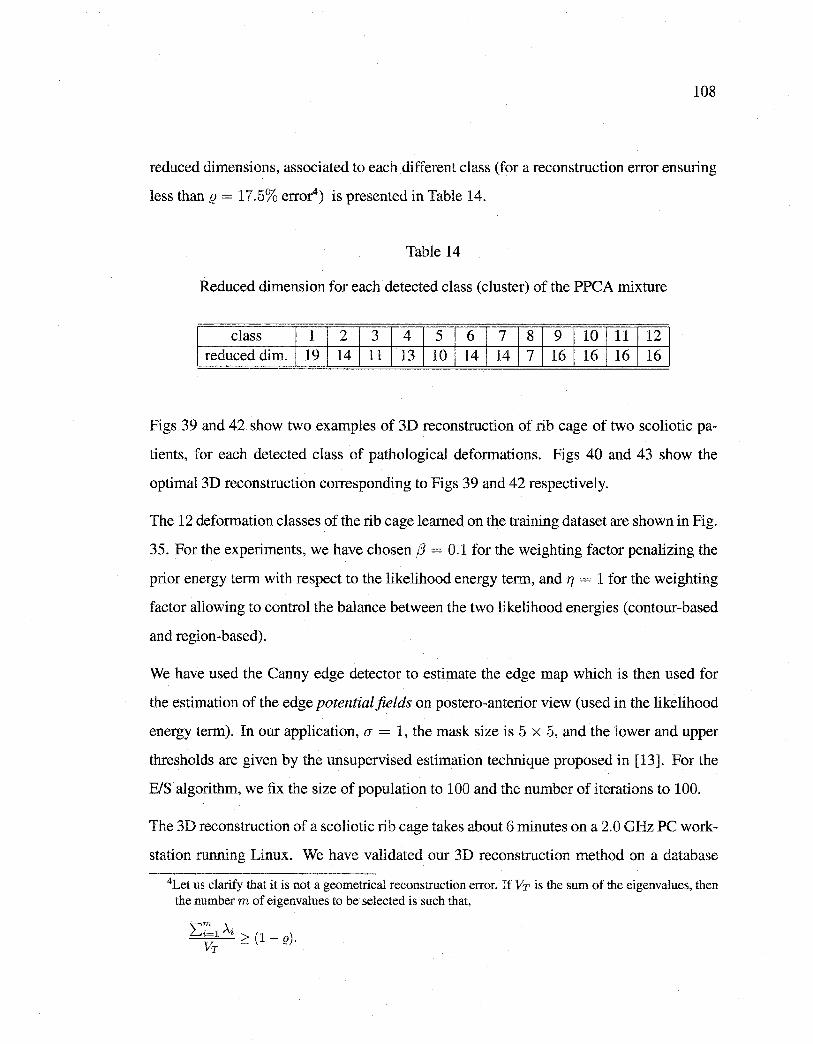
Reproduced with permission of the copyright owner. Further reproduction prohibited without permission.
108
reduced dimensions, associated to each different class (for a reconstruction error ensuring
less than (} = 17.5% erro0) is presented in Table 14.
Table 14
Reduced dimension for each detected class (cluster) of the PPCA mixture
class 1 2 3 4 5 6 7 8 9 10 11 12 reduced dim. 19 14 11 13 10 14 14 7 16 16 16 16
Figs 39 and 42 show two examples of 3D reconstruction of rib cage of two scoliotic pa
tients, for each detected class of pathological deformations. Figs 40 and 43 show the
optimal 3D reconstruction corresponding to Figs 39 and 42 respectively.
The 12 deformation classes of the rib cage learned on the training dataset are shown in Fig.
35. For the experiments, we have chosen {3 = 0.1 for the weighting factor penalizing the
prior energy term with respect to the likelihood energy term, and TJ = 1 for the weighting
factor allowing to control the balance between the two likelihood energies (contour-based
and region-based).
We have used the Canny edge detector to estimate the edge map which is then used for
the estimation of the edge potential fields on postero-anterior view ( used in the likelihood
energy term). In our application, O" = 1, the mask size is 5 x 5, and the lower and upper
thresholds are given by the unsupervised estimation technique proposed in [13]. For the
BIS algorithm, we fix the size of population to 100 and the number of iterations to 100.
The 3D reconstruction of a scoliotic rib cage takes about 6 minutes on a 2.0 GHz PC work
station running Linux. We have validated our 3D reconstruction method on a database
4Let us clarify that it is not a geometrical reconstruction error. If Vr is the sum of the eigenvalues, then the number m of eigenvalues to be selected is such that,
'\"'m À· 6 Ç; • 2 (I- e).
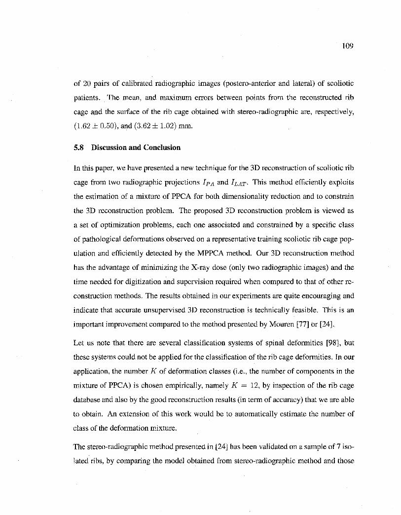
Reproduced with permission of the copyright owner. Further reproduction prohibited without permission.
109
of 20 pairs of calibrated radiographie images (postero-anterior and lateral) of scoliotic
patients. The mean, and maximum errors between points from the reconstructed rib
cage and the surface of the rib cage obtained with stereo-radiographie are, respectively,
(1.62 ± 0.50), and (3.62 ± 1.02) mm.
5.8 Discussion and Conclusion
In this paper, we have presented a new technique for the 3D reconstruction of scoliotic rib
cage from two radiographie projections !PA and hAT· This method efficiently exploits
the estimation of a mixture of PPCA for both dimensionality reduction and to constrain
the 3D reconstruction problem. The proposed 3D reconstruction problem is viewed as
a set of optimization problems, each one associated and constrained by a specifie class
of pathological deformations observed on a representative training scoliotic rib cage pop
ulation and efficiently detected by the MPPCA method. Our 3D reconstruction method
has the advantage of minimizing the X-ray dose (only two radiographie images) and the
time needed for digitization and supervision required when compared to that of other re
construction methods. The results obtained in our experiments are quite encouraging and
indicate that accurate unsupervised 3D reconstruction is technically feasible. This is an
important improvement compared to the method presented by Mouren [77] or [24].
Let us note that there are several classification systems of spinal deformities [98], but
these systems could not be applied for the classification of the rib cage deformities. In our
application, the number K of deformation classes (i.e., the number of components in the
mixture of PPCA) is chosen empirically, namely K = 12, by inspection of the rib cage
database and also by the good reconstruction results (in term of accuracy) that we are able
to obtain. An extension of this work would be to automatically estimate the number of
class of the deformation mixture.
The stereo-radiographie method presented in [24] has been validated on a sample of 7 iso
lated ribs, by comparing the model obtained from stereo-radiographie method and those
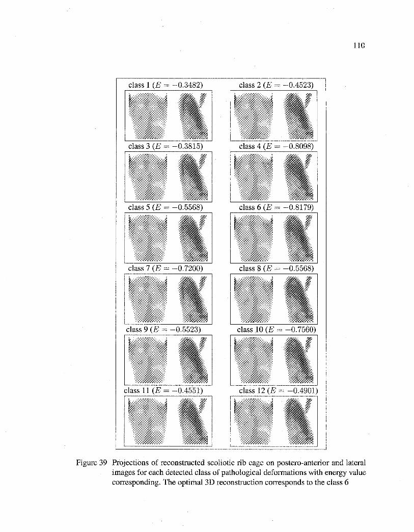
Reproduced with permission of the copyright owner. Further reproduction prohibited without permission.
110
Figure 39 Projections of reconstructed scoliotic rib cage on postero-anterior and lateral images for each detected class of pathological deformations with energy value corresponding. The optimal 3D reconstruction corresponds to the class 6
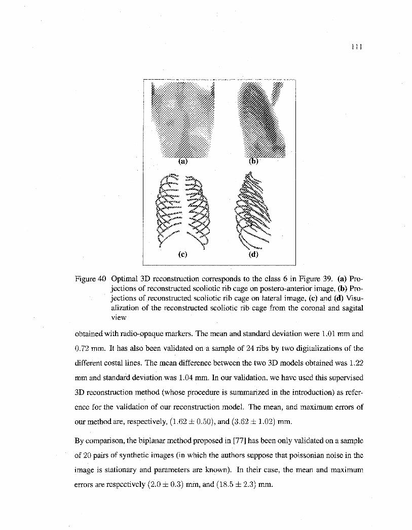
Reproduced with permission of the copyright owner. Further reproduction prohibited without permission.
111
(c) (d)
Figure 40 Optimal 3D reconstruction corresponds to the class 6 in Figure 39. (a) Projections of reconstructed scoliotic rib cage on postero-anterior image, (b) Projections of reconstructed scoliotic rib cage on lateral image, (c) and (d) Visualization of the reconstructed scoliotic rib cage from the corona! and sagital VleW
obtained with radio-opaque markers. The mean and standard deviation were 1.01 mm and
0.72 mm. It has also been validated on a sample of 24 ribs by two digitalizations of the
different costallines. The mean difference between the two 3D models obtained was 1.22
mm and standard deviation was 1.04 mm. In our validation, we have used this supervised
3D reconstruction method (whose procedure is summarized in the introduction) as refer
ence for the validation of our reconstruction model. The mean, and maximum errors of
our method are, respectively, (1.62 ± 0.50), and (3.62 ± 1.02) mm.
By comparison, the biplanar method proposed in [77] has been only validated on a sample
of 20 pairs of synthetic images (in which the authors suppose that poissonian noise in the
image is stationary and parameters are known). In their case, the mean and maximum
errors are respectively (2.0 ± 0.3) mm, and (18.5 ± 2.3) mm.
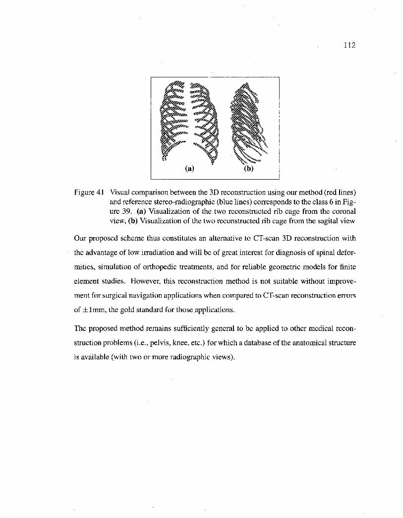
Reproduced with permission of the copyright owner. Further reproduction prohibited without permission.
112
(a) (b)
Figure 41 Visual comparison between the 3D reconstruction using our method (red lin es) and reference stereo-radiographie (blue lines) corresponds to the class 6 in Figure 39. (a) Visualization of the two reconstructed rib cage from the coronal view, (b) Visualization of the two reconstructed rib cage from the sagital view
Our proposed scheme thus constitutes an alternative to CT-scan 3D reconstruction with
the advantage of low irradiation and will be of great interest for diagnosis of spinal defor
mities, simulation of orthopedie treatments, and for reliable geometrie models for finite
element studies. However, this reconstruction method is not suitable without improve
ment for surgical navigation applications when compared to CT-scan reconstruction errors
of ±lmm, the gold standard for those applications.
The proposed method remains sufficiently general to be applied to other medical recon
struction problems (i.e., pelvis, knee, etc.) for which a database of the anatomical structure
is available (with two or more radiographie views).
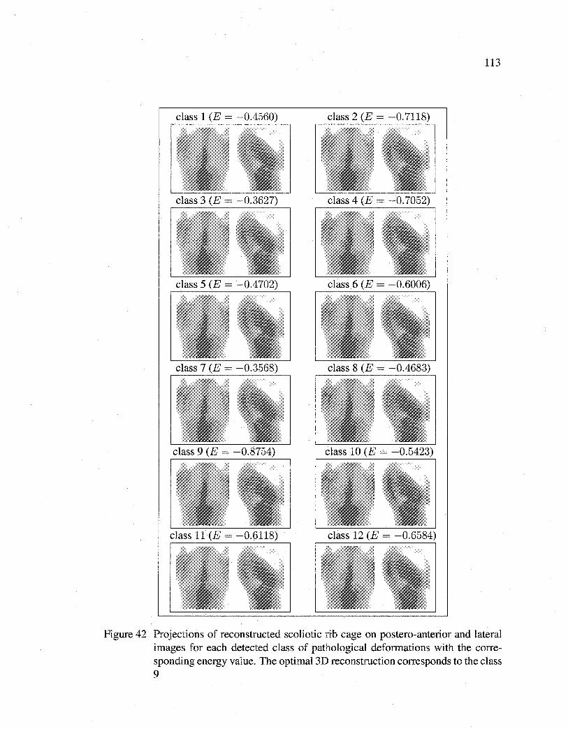
Reproduced with permission of the copyright owner. Further reproduction prohibited without permission.
113
Figure 42 Projections of reconstructed scoliotic rib cage on postero-anterior and lateral images for each detected class of pathological deformations with the corresponding energy value. The optimal 3D reconstruction corresponds to the class 9
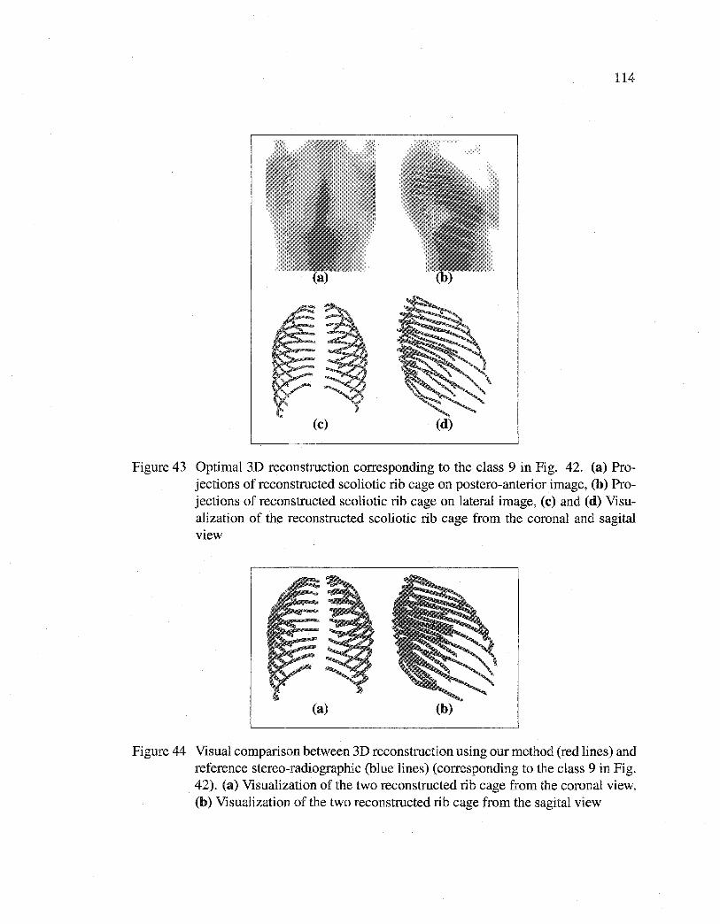
Reproduced with permission of the copyright owner. Further reproduction prohibited without permission.
114
(c) (d)
Figure 43 Optimal 3D reconstruction corresponding to the class 9 in Fig. 42. (a) Projections of reconstructed scoliotic rib cage on postero-anterior image, (b) Projections of reconstructed scoliotic rib cage on lateral image, (c) and (d) Visualization of the reconstructed scoliotic rib cage from the corona! and sagital view
(a) (b)
Figure 44 Visual comparison between 3D reconstruction using our method (red lin es) and reference stereo-radiographie (blue lines) (corresponding to the class 9 in Fig. 42). (a) Visualization of the two reconstructed rib cage from the corona! view, (b) Visualization of the two reconstructed rib cage from the sagital view
Reproduced with permission of the copyright owner. Further reproduction prohibited without permission.
DISCUSSION GÉNÉRALE
Nous avons présenté dans ce travail de recherche trois approches statistiques pour la re
construction 3D de la colonne vertébrale et de la cage thoracique scoliotiques à partir
de deux images radiographiques conventionnelles (postéro-antérieure avec incidence de
0° et latérale). Le problème de reconstruction 3D de la colonne vertébrale scoliotique a
tout d'abord été abordé par une méthode supervisée basée sur l'utilisation des contours
de vertèbres détectés sur deux images radiographiques conventionnelles et une connais
sance géométrique a priori de nature statistique de chaque vertèbre. Cette reconstruction
3D est formulée comme un problème de minimisation de fonction d'énergie résolu par
un algorithme de descente de gradient. La méthode proposée est validée sur une base de
57 vertèbres lombaires et thoraciques de 13 patients scoliotiques qui ont aussi été recon
struites par la méthode CT-scan pour des fins de comparaison. La méthode s'est avérée
performante avec une erreur moyenne de (0.71 ± 0.06) mm pour les vertèbres lombaires
et de (1.48 ± 0.27) mm pour les vertèbres thoraciques, ce qui est satisfaisant pour une
utilisation en routine clinique. Ces résultats montrent que la reconstruction des vertèbres
lombaires obtenues par notre méthode de recalage 3D/2D est plus précise que la méthode
non-stéréo-radiographique (NSCP) [75] et la méthode stéréo-radiographique [43] [76].
L'erreur moyenne est de 0.7 mm pour notre méthode, de 1.4 mm pour NSCP, de 2.4
mm pour la méthode stéréo-radiographique [76], et de 2.6 mm pour la méthode stéréo
radiographique [3]. Quelques erreurs maximums obtenues sur des apophyses épineuses
sont encore grandes (c'est-à-dire, 1' erreur maximum est de 3. 9 mm pour les vertèbres lom
baires et de 7.9 mm pour les vertèbres thoraciques). Quoique ces erreurs maximums cor
respondent à des points n'ayant pas de rôle significatif dans la planification de chirurgie, la
précision de la reconstruction est relativement acceptable, comparativement aux résultats
obtenus avec la méthode CT-scan qui est considérée comme la méthode la plus précise
de reconstruction 3D. Nous remarquons que les résultats sont meilleurs pour les vertèbres
lombaires. Pour les vertèbres thoraciques, les contours sont plus difficiles à détecter en
Reproduced with permission of the copyright owner. Further reproduction prohibited without permission.
116
raison de la présence des côtes. En plus, la taille de la base de données des vertèbres,
sur laquelle nous avons appliqué une analyse en composantes principales (ACP) pour ex
traire les déformations statistiquement admissibles, reste insuffisante et ne contient pas
toutes les déformations scoliotiques. Une grande partie de notre erreur de reconstruction
provient de la base d'apprentissage du fait que quelques déformations scoliotiques n'ont
pas été modélisées par l' ACP. Une autre partie de notre erreur de reconstruction est due à
l'erreur de reconstruction de la méthode CT-scan qui est considérée nulle dans notre pro
tocole de validation. Néanmoins, nous pouvons observer que les résultats obtenus pour
des paramètres morphométriques (importants pour la correction chirurgicale de la scol
iose) sont presque comparables à ceux obtenus par CT-scan. Contrairement aux méthodes
basées sur la numérisation des repères anatomiques [43] [75] où la reconstruction 3D
dépend de l'habilité de l'opérateur, notre méthode utilise des contours de vertèbres détec
tés automatiquement sur deux images radiographiques et l'information a priori est issue
d'une base d'apprentissage (30 normales et 30 scoliotiques par niveau vertébral) unique
et originale établie avec une grande précision. Ceci constitue une contribution non nég
ligeable apportée par notre méthode. Notons que les paramètres de déformations obtenues
par la reconstruction 3D peuvent être utilisés pour étudier la scoliose. Notre méthode
s'applique à d'autres structures pourvu qu'une base de données de la structure en question
soit disponible.
La méthode présentée est supervisée et ne tient pas compte des paramètres de la vertèbre
reconstruite à 1' étape précédente. Pour pallier à cette limitation, nous avons présenté une
autre méthode originale de reconstruction 3D hiérarchique, statistique et non supervisée
des colonnes vertébrales scoliotiques basée sur l'utilisation des contours des vertèbres
détectés sur deux images radiographiques conventionnelles et une connaissance globale
hiérarchique a priori comprenant la structure géométrique de la colonne vertébrale et de
chaque niveau vertébral. La nouvelle méthode est basée sur la spécification de deux mod
èles 3D statistiques. Le premier, un modèle géométrique sur lequel des déformations
linéaires globales admissibles sont définies, est utilisé pour une reconstruction grossière
Reproduced with permission of the copyright owner. Further reproduction prohibited without permission.
117
de la colonne vertébrale. Une reconstruction 3D précise est alors réalisée pour chaque
niveau vertébral par un deuxième modèle de vertèbre sur lequel des déformations non
linéaires admissibles (déformations locales) sont définies. Cette reconstruction 3D est for
mulée comme un double problème de minimisation de fonction d'énergie efficacement
résolus par un algorithme stochastique d'exploration/selection. La méthode proposée est
validée sur la même base que la première méthode et s'est avérée performante avec une
erreur moyenne de (1.45 ± 1.46) mm pour les vertèbres lombaires et de (1.27 ± 1.29) mm
pour les vertèbres thoraciques, ce qui est aussi satisfaisant pour une utilisation en routine
clinique.
La reconstruction 3D nécessite un temps de calcul de l'ordre de 28 secondes sur une
station de travail PC à 2.0 GHz sous Linux pour une vertèbre. En comparant ces ré
sultats à ceux de la méthode précédente [8], nous constatons que la précision de la pre
mière est meilleure que celle de la deuxième méthode. Ceci est dû au fait que la méth
ode précédente [8] est supervisée et exige la connaissance de la position de six repères
anatomiques stéréo-correspondants par vertèbre (centroïdes des plateaux vertébraux, som
mets des pédicules) sur les deux images radiographiques pour l'initialisation de chaque
vertèbre dans l'environnement radiographique en vue d'une reconstruction 3D. Par exem
ple, la reconstruction 3D du segment de vertèbres (L5/ ... /Tl) nécessite la connaissance
de la position de 102 repères anatomiques alors qu'avec cette deuxième méthode, il suffit
de connaître la position du centroïde des plateaux vertébraux de la première vertèbre du
segment sur les deux images radiographiques. Une contribution importante apportée par
cette deuxième méthode est que la reconstruction 3D est non supervisée et permet une
reconstruction 3D des segments de la colonne vertébrale. Aussi, cette deuxième méthode
s'applique à d'autres structures pourvu qu'une base de données de la structure en question
soit disponible.
Finalement, nous avons présenté une méthode originale de reconstruction 3D non super
visée des cages thoraciques scoliotiques à partir de deux images radiographiques con-
Reproduced with permission of the copyright owner. Further reproduction prohibited without permission.
118
ventionnelles (postéro-antérieure avec incidence de oo et latérale). Dans ce modèle, nous
avons posé l'hypothèse que chacune des formes de cage thoracique associée à une patholo
gie de scoliose possible, et liée à une déformation globale et spécifique de la colonne
vertébrale, est distribué dans une classe de déformation spécifique, pour laquelle nous
avons ensuite défini une réduction de dimensionnalité linéaire classique telle qu'une tech
nique d' ACP probabiliste. Dans ce contexte, nous avons utilisé un mélange d' ACP prob
abiliste dont chaque composante de ce mélange représente un type de déformation parti
culière de scoliose. Les paramètres du mélange d' ACP probabiliste sont estimés par une
version stochastique de l'algorithme EM (Expectation, Maximization) appelée SEM. La
reconstruction 3D optimale correspond à la classe de la déformation et aux paramètres
menant à l'énergie minimale d'une fonction d'énergie heuristiquement définie. Due à
l'absence d'une base de cages thoraciques scoliotiques numérisées, la méthode proposée
a été validée sur un échantillon de 20 paires d'images radiographiques et comparée aux
reconstructions 3D issues de la méthode stéréo-radiographique. Une erreur moyenne de
(1.62 ± 0.50) mm a été obtenue sur les distances point-surface entre le modèle reconstruit
avec notre méthode et le modèle issu de la reconstruction stéréo-radiographique.
La reconstruction 3D d'une cage thoracique scoliotique nécessite un temps de calcul de
l'ordre de 6 minutes sur une station de travail PC à 2.0 GHz sous Linux. Une contribu
tion importante apportée par cette méthode est que d'une part la reconstruction 3D est
non supervisée et utilise seulement deux images radiographiques (postéro-antérieure avec
incidence de oo et latérale) ainsi qu'une base d'apprentissage de 532 cages thoraciques
scoliotiques, unique dans la littérature. D'autre part, l'utilisation de mélange d' ACP prob
abiliste, dont les paramètres sont estimés par l'algorithme SEM (Stochastic, Expectation,
Maximization), pour la définition d'un mélange de modèle a priori de formes 3D pour
la régularisation de notre problème de reconstruction 3D n'avait été jusqu'à maintenant
jamais été utilisée. En plus de la reconstruction 3D, cette méthode permet un classement
implicite et probabiliste de chacune des pathologies scoliotiques existantes dans la base
d'apprentissage.
Reproduced with permission of the copyright owner. Further reproduction prohibited without permission.
119
La qualité des contours extraits des deux images radiographiques est la principale limite
des approches statistiques proposées dans cette thèse. Ce qui explique les erreurs de re
construction observées au niveau des vertèbres et des cages thoraciques. Ainsi, le manque
de visibilité dans les images radiographiques latérales rend leur segmentation très difficile.
Outre cette limite, la taille de la base d'apprentissage par niveau vertébral ne permet pas
de représenter toutes les déformations possibles générées par la scoliose.
Principales contributions
Dans le premier article (cf. Chap. 2), nous proposons une méthode statistique de recon
struction 3D des vertèbres scoliotiques à partir de I pA et hAT [7]. Cette méthode est basée
sur une connaissance a priori globale de la variabilité géométrique de chaque vertèbre sco
liotique apprise sur une base d'apprentissage de vertèbres. Le positionnement initial du
modèle déformable statistique dans l'espace radiographique est réalisé par l'utilisation de
six repères anatomiques (centroïdes des plateaux vertébraux, sommets des pédicules). La
méthode de reconstruction proposée consiste à ajuster les projections (postéro-antérieure
et latérale) du contour externe de ce modèle a priori 3D de chaque niveau vertébral avec
les contours correspondants préalablement segmentés sur les deux vues radiographiques.
Cette reconstruction 3D est formulée comme un problème de minimisation de fonction
d'énergie résolue par un algorithme de descente de gradient simplifié. Une contribution
non négligeable apportée par cette méthode est que, d'une part, l'information utilisée est
caractérisée par des contours de vertèbres détectés sur deux images radiographiques et
l'information a priori est issue d'une base d'apprentissage (30 normales et 30 scoliotiques
par niveau vertébral) unique et originale établie avec une grande précision [82]. D'autre
part, nous avons adapté l'approche de Cootes pour contraindre le problème mal-posé de
recalage des modèles 3D de vertèbres scoliotiques sur des images radiographiques bi
planaires.
La méthode présentée dans le premier article est supervisée et ne tient pas compte des
paramètres de la vertèbre reconstruite à 1' étape précédente. Pour pallier cette limitation,
Reproduced with permission of the copyright owner. Further reproduction prohibited without permission.
120
nous présentons dans le deuxième article (cf. Chap. 3) une nouvelle méthode de recon
struction 3D hiérarchique statistique non supervisée des colonnes vertébrales scoliotiques
basée sur 1 'utilisation I pA et hAT et une connaissance globale hiérarchique a priori com
prenant la structure géométrique de la colonne vertébrale et de chaque niveau vertébral
[8]. La nouvelle méthode est basée sur les spécifications de deux modèles 3D statistiques.
Le premier, un modèle géométrique sur lequel des déformations linéaires globales admis
sibles sont définies, est utilisé pour une reconstruction grossière de la colonne vertébrale.
Une reconstruction 3D précise est alors réalisée pour chaque niveau vertébral par un deux
ième modèle de vertèbre sur lequel des déformations non linéaires admissibles (défor
mations locales) sont définies. Cette deuxième étape consiste à ajuster les projections
(postéro-antérieure et latérale) du contour externe de ce modèle a priori 3D de chaque
niveau vertébral avec les contours du niveau correspondant préalablement segmentés sur
les deux vues radiographiques. Cette reconstruction 3D est formulée comme un double
problème de minimisation de fonction d'énergie efficacement résolu par un algorithme
d'optimisation stochastique. Une contribution importante apportée par cette deuxième
méthode est que la reconstruction 3D est obtenue par combinaison de deux modèles 3D
statistiques. Un modèle 3D grossier est utilisé pour contraindre un modèle 3D plus pré
cis. Cette méthode est de plus non supervisée et permet une reconstruction 3D precise des
segments de vertèbres.
La méthode présentée dans le deuxième article n'est pas applicable directement aux cages
thoraciques scoliotiques du fait de leur structure géométrique particulière et surtout, des
déformations pathologiques associées à celle-ci, étroitement liée à la déformation glob
ale de la colonne vertébrale elle-même. En plus, les données associées à chacune des
cages thoraciques de notre base d'apprentissage ne sont pas linéairement distribuées dans
1' espace des formes tridimensionnelles possibles. L' ACP ne peut ainsi être efficacement
utilisé. Dans le modèle que nous avons proposé, nous avons supposé moins restrictive
ment que chacune des formes de cage thoracique est liée à une déformation globale et
spécifique de la colonne vertébrale. Ces formes sont distribués dans une classe ou une
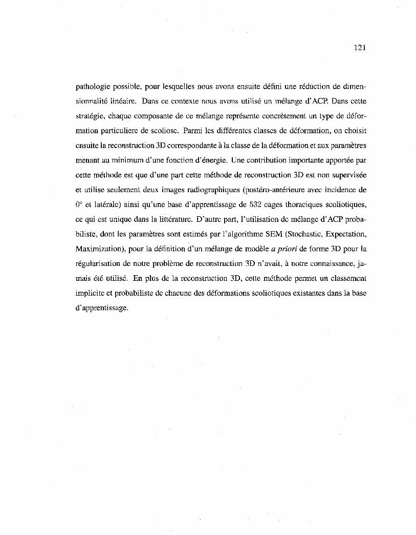
Reproduced with permission of the copyright owner. Further reproduction prohibited without permission.
121
pathologie possible, pour lesquelles nous avons ensuite défini une réduction de dimen
sionnalité linéaire. Dans ce contexte nous avons utilisé un mélange d' ACP. Dans cette
stratégie, chaque composante de ce mélange représente concrètement un type de défor
mation particuliere de scoliose. Parmi les différentes classes de déformation, on choisit
ensuite la reconstruction 3D correspondante à la classe de la déformation et aux paramètres
menant au minimum d'une fonction d'énergie. Une contribution importante apportée par
cette méthode est que d'une part cette méthode de reconstruction 3D est non supervisée
et utilise seulement deux images radiographiques (postéro-antérieure avec incidence de
oo et latérale) ainsi qu'une base d'apprentissage de 532 cages thoraciques scoliotiques,
ce qui est unique dans la littérature. D'autre part, l'utilisation de mélange d' ACP proba
biliste, dont les paramètres sont estimés par l'algorithme SEM (Stochastic, Expectation,
Maximization), pour la définition d'un mélange de modèle a priori de forme 3D pour la
régularisation de notre problème de reconstruction 3D n'avait, à notre connaissance, ja
mais été utilisé. En plus de la reconstruction 3D, cette méthode permet un classement
implicite et probabiliste de chacune des déformations scoliotiques existantes dans la base
d'apprentissage.
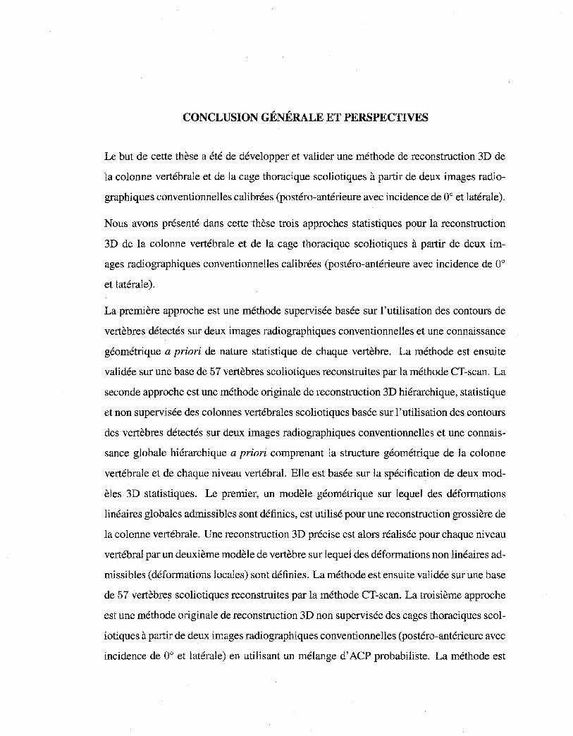
Reproduced with permission of the copyright owner. Further reproduction prohibited without permission.
CONCLUSION GÉNÉRALE ET PERSPECTIVES
Le but de cette thèse a été de développer et valider une méthode de reconstruction 3D de
la colonne vertébrale et de la cage thoracique scoliotiques à partir de deux images radio
graphiques conventionnelles calibrées (postéro-antérieure avec incidence de oo et latérale).
Nous avons présenté dans cette thèse trois approches statistiques pour la reconstruction
3D de la colonne vertébrale et de la cage thoracique scoliotiques à partir de deux im
ages radiographiques conventionnelles calibrées (postéro-antérieure avec incidence de oo et latérale).
La première approche est une méthode supervisée basée sur l'utilisation des contours de
vertèbres détectés sur deux images radiographiques conventionnelles et une connaissance
géométrique a priori de nature statistique de chaque vertèbre. La méthode est ensuite
validée sur une base de 57 vertèbres scoliotiques reconstruites par la méthode CT-scan. La
seconde approche est une méthode originale de reconstruction 3D hiérarchique, statistique
et non supervisée des colonnes vertébrales scoliotiques basée sur l'utilisation des contours
des vertèbres détectés sur deux images radiographiques conventionnelles et une connais
sance globale hiérarchique a priori comprenant la structure géométrique de la colonne
vertébrale et de chaque niveau vertébral. Elle est basée sur la spécification de deux mod
èles 3D statistiques. Le premier, un modèle géométrique sur lequel des déformations
linéaires globales admissibles sont définies, est utilisé pour une reconstruction grossière de
la colonne vertébrale. Une reconstruction 3D précise est alors réalisée pour chaque niveau
vertébral par un deuxième modèle de vertèbre sur lequel des déformations non linéaires ad
missibles (déformations locales) sont définies. La méthode est ensuite validée sur une base
de 57 vertèbres scoliotiques reconstruites par la méthode CT-scan. La troisième approche
est une méthode originale de reconstruction 3D non supervisée des cages thoraciques scol
iotiques à partir de deux images radiographiques conventionnelles (postéro-antérieure avec
incidence de oo et latérale) en utilisant un mélange d' ACP probabiliste. La méthode est
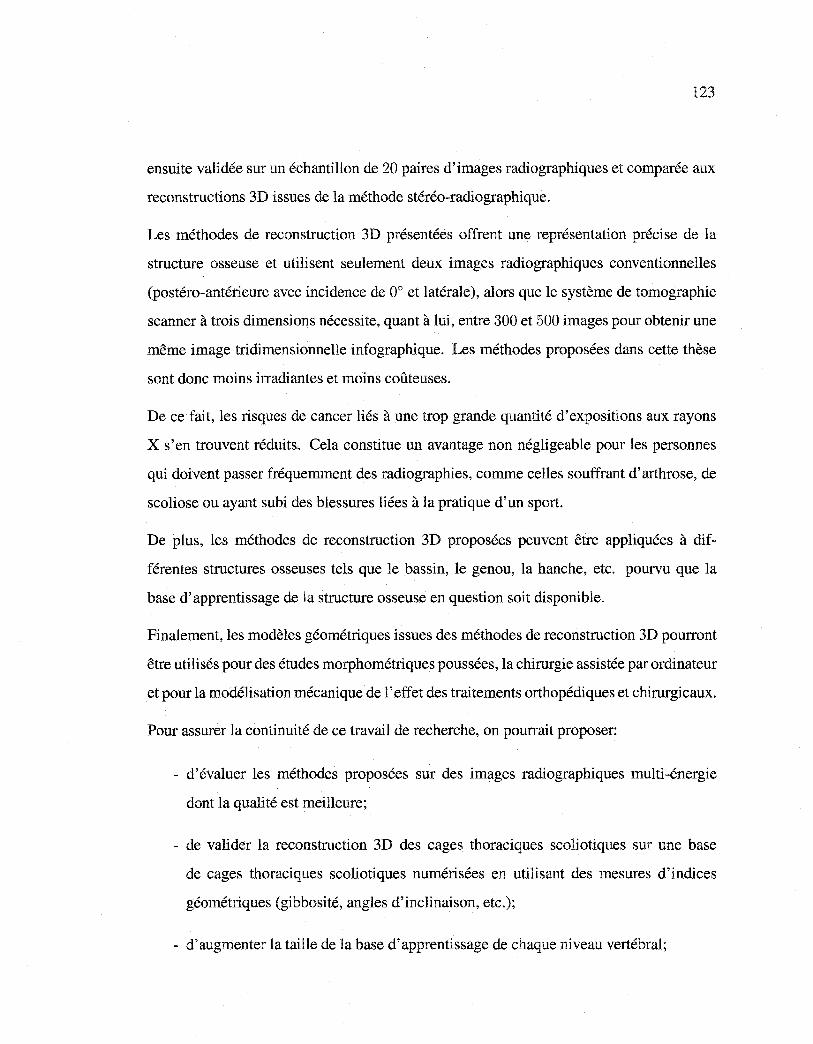
Reproduced with permission of the copyright owner. Further reproduction prohibited without permission.
123
ensuite validée sur un échantillon de 20 paires d'images radiographiques et comparée aux
reconstructions 3D issues de la méthode stéréo-radiographique.
Les méthodes de reconstruction 3D présentées offrent une représentation précise de la
structure osseuse et utilisent seulement deux images radiographiques conventionnelles
(postéro-antérieure avec incidence de oo et latérale), alors que le système de tomographie
scanner à trois dimensions nécessite, quant à lui, entre 300 et 500 images pour obtenir une
même image tridimensionnelle infographique. Les méthodes proposées dans cette thèse
sont donc moins irradiantes et moins coûteuses.
De ce fait, les risques de cancer liés à une trop grande quantité d'expositions aux rayons
X s'en trouvent réduits. Cela constitue un avantage non négligeable pour les personnes
qui doivent passer fréquemment des radiographies, comme celles souffrant d'arthrose, de
scoliose ou ayant subi des blessures liées à la pratique d'un sport.
De plus, les méthodes de reconstruction 3D proposées peuvent être appliquées à dif
férentes structures osseuses tels que le bassin, le genou, la hanche, etc. pourvu que la
base d'apprentissage de la structure osseuse en question soit disponible.
Finalement, les modèles géométriques issues des méthodes de reconstruction 3D pourront
être utilisés pour des études morphométriques poussées, la chirurgie assistée par ordinateur
et pour la modélisation mécanique de 1' effet des traitements orthopédiques et chirurgicaux.
Pour assurer la continuité de ce travail de recherche, on pourrait proposer:
- d'évaluer les méthodes proposées sur des images radiographiques multi-énergie
dont la qualité est meilleure;
- de valider la reconstruction 3D des cages thoraciques scoliotiques sur une base
de cages thoraciques scoliotiques numérisées en utilisant des mesures d'indices
géométriques (gibbosité, angles d'inclinaison, etc.);
- d'augmenter la taille de la base d'apprentissage de chaque niveau vertébral;
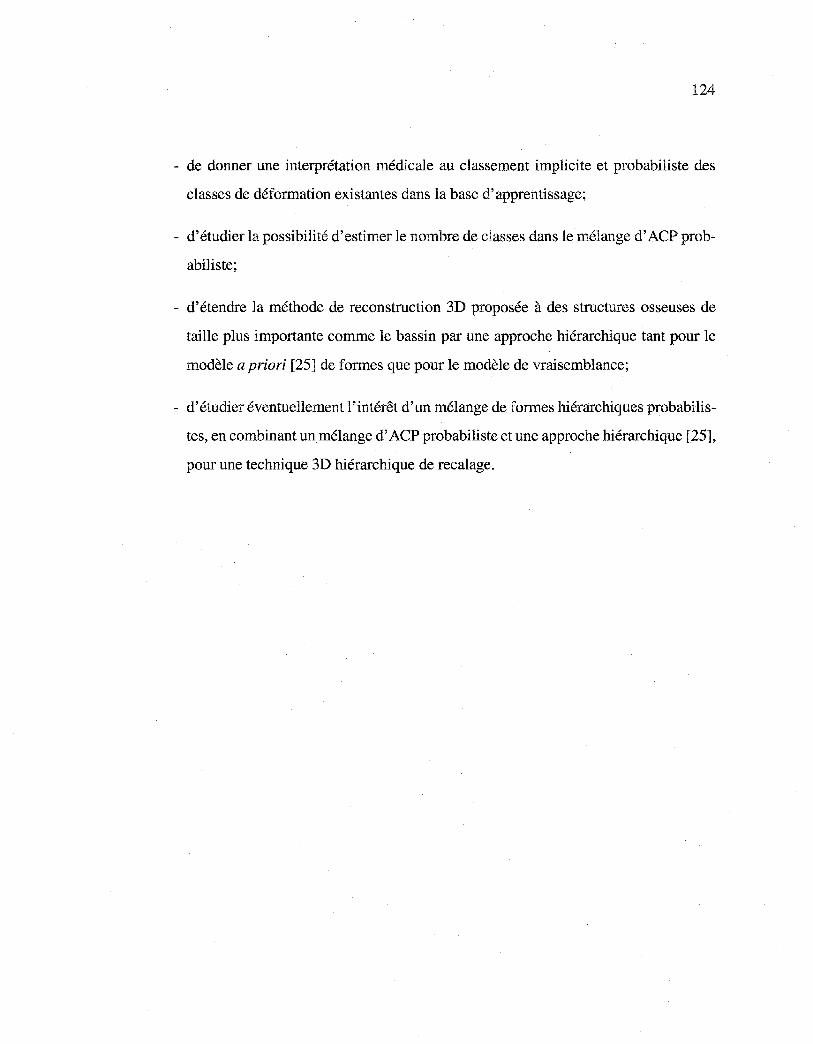
Reproduced with permission of the copyright owner. Further reproduction prohibited without permission.
124
- de donner une interprétation médicale au classement implicite et probabiliste des
classes de déformation existantes dans la base d'apprentissage;
- d'étudier la possibilité d'estimer le nombre de classes dans le mélange d' ACP prob
abiliste;
- d'étendre la méthode de reconstruction 3D proposée à des structures osseuses de
taille plus importante comme le bassin par une approche hiérarchique tant pour le
modèle a priori [25] de formes que pour le modèle de vraisemblance;
- d'étudier éventuellement l'intérêt d'un mélange de formes hiérarchiques probabilis
tes, en combinant un mélange d' ACP probabiliste et une approche hiérarchique [25],
pour une technique 3D hiérarchique de recalage.

Reproduced with permission of the copyright owner. Further reproduction prohibited without permission.
ANNEXES

Reproduced with permission of the copyright owner. Further reproduction prohibited without permission.
ANNEXE1
GLOSSAIRE DE TERMES
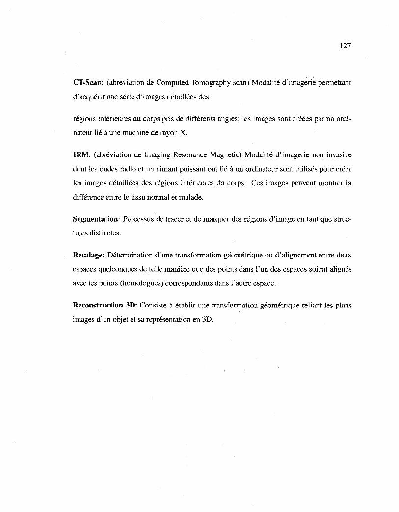
Reproduced with permission of the copyright owner. Further reproduction prohibited without permission.
127
CT-Scan: (abréviation de Computed Tomography scan) Modalité d'imagerie permettant
d'acquérir une série d'images détaillées des
régions intérieures du corps pris de différents angles; les images sont créées par un ordi
nateur lié à une machine de rayon X.
IRM: (abréviation de Imaging Resonance Magnetic) Modalité d'imagerie non invasive
dont les ondes radio et un aimant puissant ont lié à un ordinateur sont utilisés pour créer
les images détaillées des régions intérieures du corps. Ces images peuvent montrer la
différence entre le tissu normal et malade.
Segmentation: Processus de tracer et de marquer des régions d'image en tant que struc
tures distinctes.
Recalage: Détermination d'une transformation géométrique ou d'alignement entre deux
espaces quelconques de telle manière que des points dans l'un des espaces soient alignés
avec les points (homologues) correspondants dans l'autre espace.
Reconstruction 3D: Consiste à établir une transformation géométrique reliant les plans
images d'un objet et sa représentation en 3D.

Reproduced with permission of the copyright owner. Further reproduction prohibited without permission.
ANNEXE2
ANATOMIE
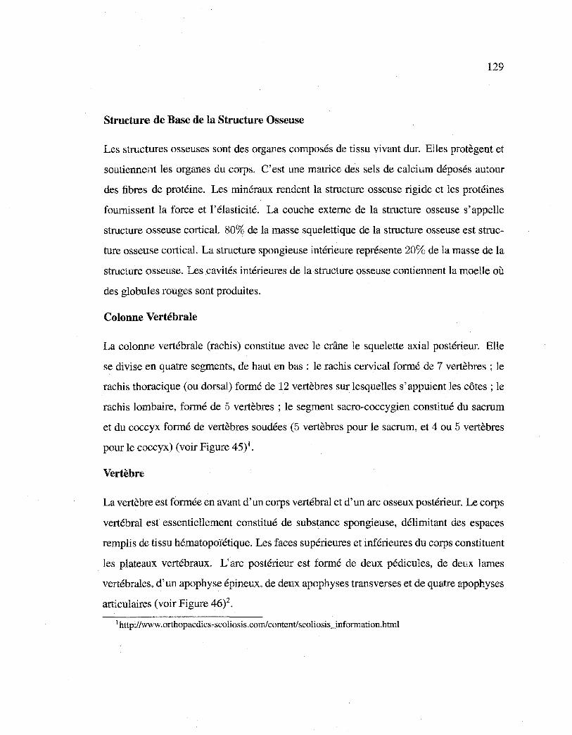
Reproduced with permission of the copyright owner. Further reproduction prohibited without permission.
129
Structure de Base de la Structure Osseuse
Les structures osseuses sont des organes composés de tissu vivant dur. Elles protègent et
soutiennent les organes du corps. C'est une matrice des sels de calcium déposés autour
des fibres de protéine. Les minéraux rendent la structure osseuse rigide et les protéines
fournissent la force et l'élasticité. La couche externe de la structure osseuse s'appelle
structure osseuse cortical. 80% de la masse squelettique de la structure osseuse est struc
ture osseuse cortical. La structure spongieuse intérieure représente 20% de la masse de la
structure osseuse. Les cavités intérieures de la structure osseuse contiennent la moelle où
des globules rouges sont produites.
Colonne Vertébrale
La colonne vertébrale (rachis) constitue avec le crâne le squelette axial postérieur. Elle
se divise en quatre segments, de haut en bas : le rachis cervical formé de 7 vertèbres ; le
rachis thoracique (ou dorsal) formé de 12 vertèbres sur lesquelles s'appuient les côtes; le
rachis lombaire, formé de 5 vertèbres ; le segment sacra-coccygien constitué du sacrum
et du coccyx formé de vertèbres soudées (5 vertèbres pour le sacrum, et 4 ou 5 vertèbres
pour le coccyx) (voir Figure 45)1•
Vertèbre
La vertèbre est formée en avant d'un corps vertébral et d'un arc osseux postérieur. Le corps
vertébral est essentiellement constitué de substance spongieuse, délimitant des espaces
remplis de tissu hématopoïétique. Les faces supérieures et inférieures du corps constituent
les plateaux vertébraux. L'arc postérieur est formé de deux pédicules, de deux lames
vertébrales, d'un apophyse épineux, de deux apophyses transverses et de quatre apophyses
articulaires (voir Figure 46)2•
1 http://www.orthopaedics-scoliosis.com/content/scoliosis_information.html
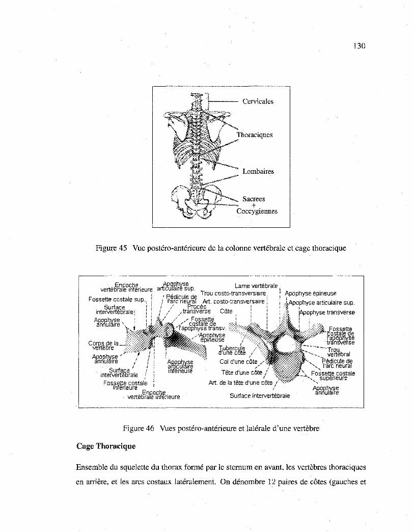
Reproduced with permission of the copyright owner. Further reproduction prohibited without permission.
Cervicales
Lombaires
Sacrees +
Coccygiennes
Figure 45 Vue postéro-antérieure de la colonne vertébrale et cage thoracique
_ 5Enco.ch~ . verte rate mfeneure
Fossette costale sup., . Surfa,c;e . · tnteNerteorale ~
Afn°rfu~~fr~
Coro$. 5de la__ .
ve"rte re
Afn°rfu1Mfr~ inte~rtf{b~ale Fos.sette costale
1nteneure
aJç_Pu~g~ss~p. Lame vertébrale 1 Pédicule de Trou costo-transversa1re: / l'arc neural Art. costo-transv-ersa1re ; 1 / Procès • 1 f / transverse Côte ! 1
/ / F oss1ette
"" costa ede l'apophyse transv.
,. 1
1
Tubercwle d'une cote Col d'une côte
Tête d'une côte
Art. de la tête d'une côte
Enco.ch!'l vertétirate Inferieure
1
Surface intervertébrale
Figure 46 Vues postéro-antérieure et latérale d'une vertèbre
Cage Thoracique
130
Ensemble du squelette du thorax formé par le sternum en avant, les vertèbres thoraciques
en arrière, et les arcs costaux latéralement. On dénombre 12 paires de côtes (gauches et
Reproduced with permission of the copyright owner. Further reproduction prohibited without permission.
131
droites) réparties en trois catégories : les vraies côtes, soit les 7 premières (Cl à C7),
chacune s'articulant directement avec le sternum par le biais d'un cartilage; les fausses
côtes (C8 à ClO), rattachées au sternum par un cartilage commun; les côtes flottantes
(Cll et C12) dont l'extrémité antérieure reste libre (voir Figure 47)2•
Clavicule, extrémité aeromiele 1 1 .;, ..
dl"-·
·r-... : j 1
'
Acromion , .!! Épine"' · JI!' ·,...,. 8" l Fosse · E i SOUH,plneuse 0,
lRebord '""'''"''··-··
11 ième côte -
1 ière wrtèbre lombaire, apophyse costale
6 !ème vertèbre cervicale ·r, ~ 1 Ière vertèbre · · ~ thoracique
1lère côte
12 ième vertèbre thoracique
Figure 4 7 Vue postéro-antérieure de la cage thoracique
2http://www.cegep-baie-comeau.qc.calbio/Anatomie%20corps%20humain%20cd/dos.html

Reproduced with permission of the copyright owner. Further reproduction prohibited without permission.
ANNEXE3
ALGORITHMES D'ALIGNEMENT DE FORMES
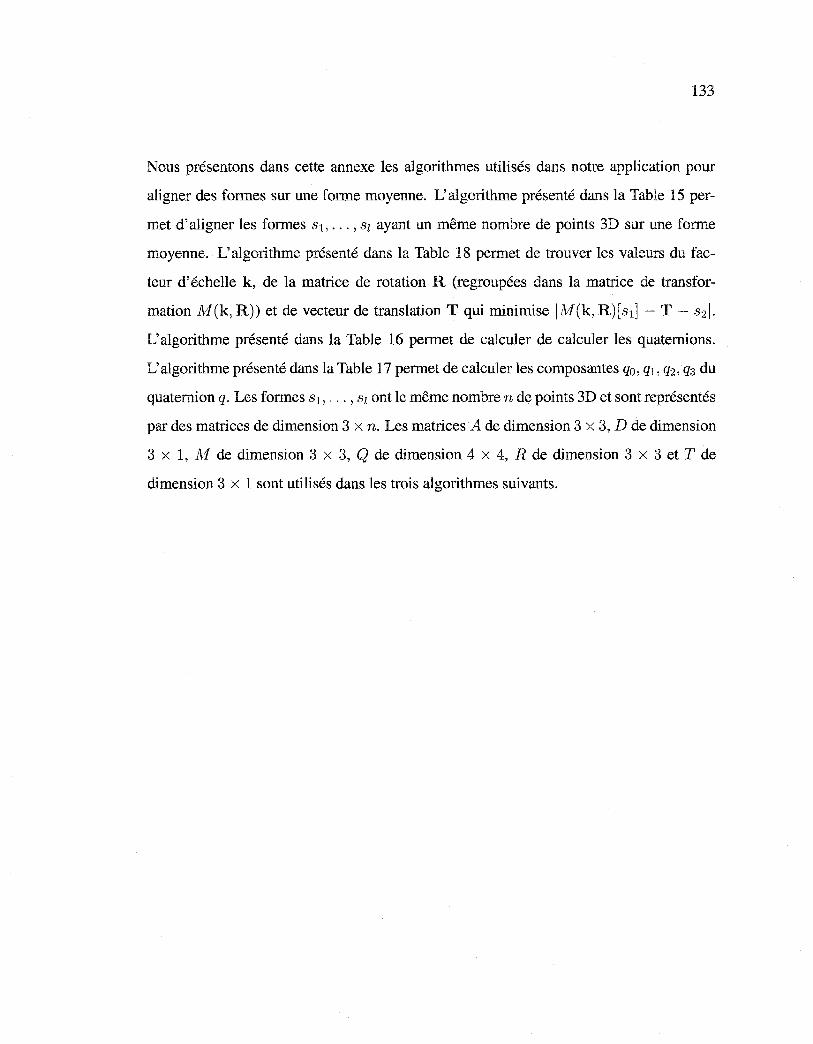
Reproduced with permission of the copyright owner. Further reproduction prohibited without permission.
133
Nous présentons dans cette annexe les algorithmes utilisés dans notre application pour
aligner des formes sur une forme moyenne. L'algorithme présenté dans la Table 15 per
met d'aligner les formes s1 , ... , s1 ayant un même nombre de points 3D sur une forme
moyenne. L'algorithme présenté dans la Table 18 permet de trouver les valeurs du fac
teur d'échelle k, de la matrice de rotation R (regroupées dans la matrice de transfor
mation M(k, R)) et de vecteur de translation T qui minimise \M(k, R)[s1] - T- s2 \.
L'algorithme présenté dans la Table 16 permet de calculer de calculer les quaternions.
L'algorithme présenté dans la Table 17 permet de calculer les composantes q0 , q1 , q2 , q3 du
quaternion q. Les formes s11 ••• , s1 ont le même nombre n de points 3D et sont représentés
par des matrices de dimension 3 x n. Les matrices A de dimension 3 x 3, D de dimension
3 x 1, M de dimension 3 x 3, Q de dimension 4 x 4, R de dimension 3 x 3 et T de
dimension 3 x 1 sont utilisés dans les trois algorithmes suivants.
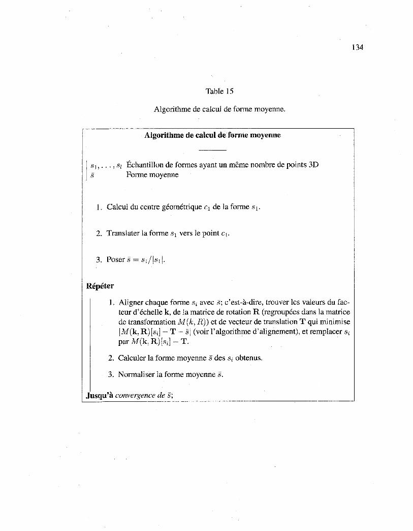
Reproduced with permission of the copyright owner. Further reproduction prohibited without permission.
Table 15
Algorithme de calcul de forme moyenne.
Algorithme de calcul de forme moyenne
1 S~1 , ... , Sz Échantillon de formes ayant un même nombre de points 3D
Forme moyenne
1. Calcul du centre géométrique c1 de la forme s 1 .
2. Translater la forme s1 vers le point c1.
Répéter
1. Aligner chaque forme si avec s; c'est-à-dire, trouver les valeurs du facteur d'échelle k, de la matrice de rotation R (regroupées dans la matrice de transformation M(k, R)) et de vecteur de translation T qui minimise IM(k, R)[si]- T- si (voir l'algorithme d'alignement), et remplacer si
par M(k, R)[si]- T.
2. Calculer la forme moyenne s des si obtenus.
3. Normaliser la forme moyenne s.
Jusqu'à convergence de s;
134
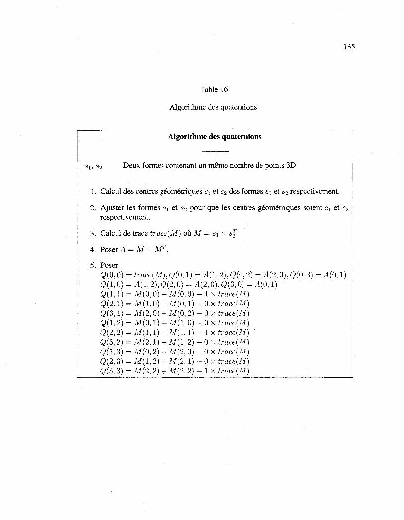
Reproduced with permission of the copyright owner. Further reproduction prohibited without permission.
135
Table 16
Algorithme des quaternions.
Algorithme des quaternions
Deux formes contenant un même nombre de points 3D
1. Calcul des centres géométriques c1 et c2 des formes 3 1 et 3 2 respectivement.
2. Ajuster les formes 3 1 et 3 2 pour que les centres géométriques soient c1 et c2
respectivement.
3. Calcul de trace trace(M) où M = 3 1 x 3§.
4. Poser A = M - MT.
5. Poser Q(O, 0) = trace(M), Q(O, 1) = A(1, 2), Q(O, 2) = A(2, 0), Q(O, 3) = A(O, 1) Q(1, 0) = A(1, 2), Q(2, 0) = A(2, 0), Q(3, 0) = A(O, 1) Q(1, 1) = M(O, 0) + M(O, 0)- 1 x trace(M) Q(2, 1) = M(1, 0) + M(O, 1)- 0 x trace(M) Q(3, 1) = M(2, 0) + M(O, 2)- 0 x trace(M) Q(1, 2) = M(O, 1) + M(1, 0)- 0 x trace(M) Q(2, 2) = M(1, 1) + M(1, 1) - 1 x trace(M) Q(3, 2) = M(2, 1) + M(1, 2) - 0 x trace(M) Q(1, 3) = M(O, 2) + M(2, 0)- 0 x trace(M) Q(2, 3) = N/(1, 2) + M(2, 1)- 0 x trace(M) Q(3, 3) = M(2, 2) + M(2, 2)- 1 x trace(M)
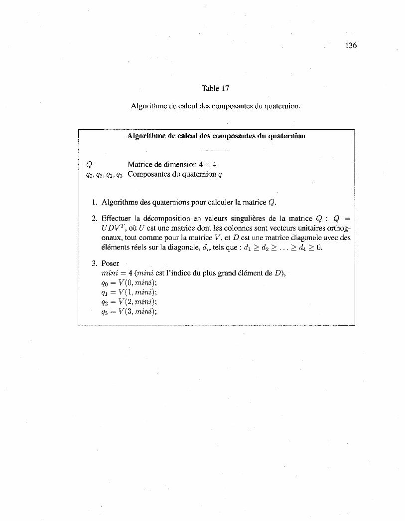
Reproduced with permission of the copyright owner. Further reproduction prohibited without permission.
136
Table 17
Algorithme de calcul des composantes du quaternion.
Algorithme de calcul des composantes du quaternion
1
Q Matrice de dimension 4 x 4 qo, q1, q2, q3 Composantes du quaternion q
1. Algorithme des quaternions pour calculer la matrice Q.
2. Effectuer la décomposition en valeurs singulières de la matrice Q : Q =
U DVT, où U est une matrice dont les colonnes sont vecteurs unitaires orthogonaux, tout comme pour la matrice V, et D est une matrice diagonale avec des éléments réels sur la diagonale, di, tels que: d1 ~ d2 ~ ... ~ d4 ~ O.
3. Poser mini = 4 (mini est l'indice du plus grand élément de D), qo = V(O, mini);
q1 = V(l, mini); q2 = V(2, mini);
q3 = V(3, mini);
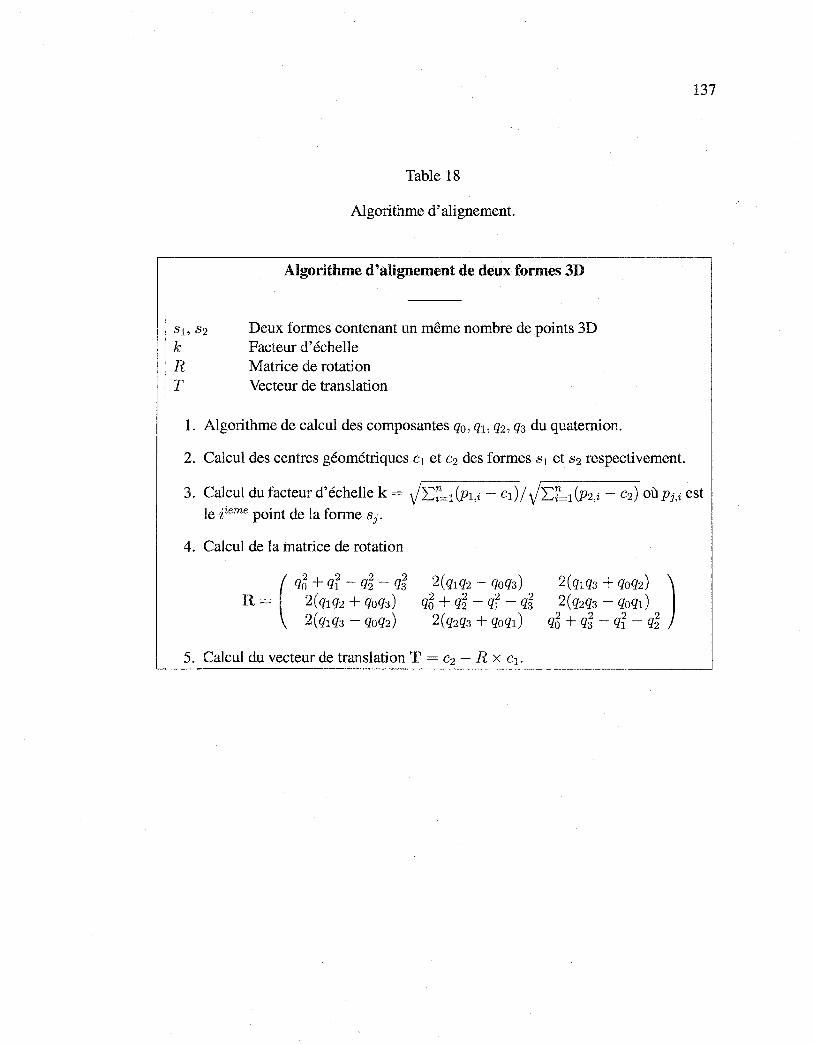
Reproduced with permission of the copyright owner. Further reproduction prohibited without permission.
137
Table 18
Algorithme d'alignement.
Algorithme d'alignement de deux formes 3D
s1, s 2 Deux formes contenant un même nombre de points 3D k Facteur d'échelle R Matrice de rotation T Vecteur de translation
1. Algorithme de calcul des composantes q0 , q1, q2 , q3 du quaternion.
2. Calcul des centres géométriques c1 et c2 des formes s 1 et s2 respectivement.
3. Calcul du facteur d'échelle k = Jz:.~=l (Pl,i - c1) / Jz:.~=l (Pz,i - cz) où Pj,i est le iieme point de la forme Sj.
4. Calcul de la matrice de rotation
2(qlq2- qoq3) q5 + q~ - qr - q~
2(qzq3 + qoql)
5. Calcul du vecteur de translation T = c2 - R x c1 .

Reproduced with permission of the copyright owner. Further reproduction prohibited without permission.
ANNEXE4
RÉSULTATS COMPLÉMENTAIRES
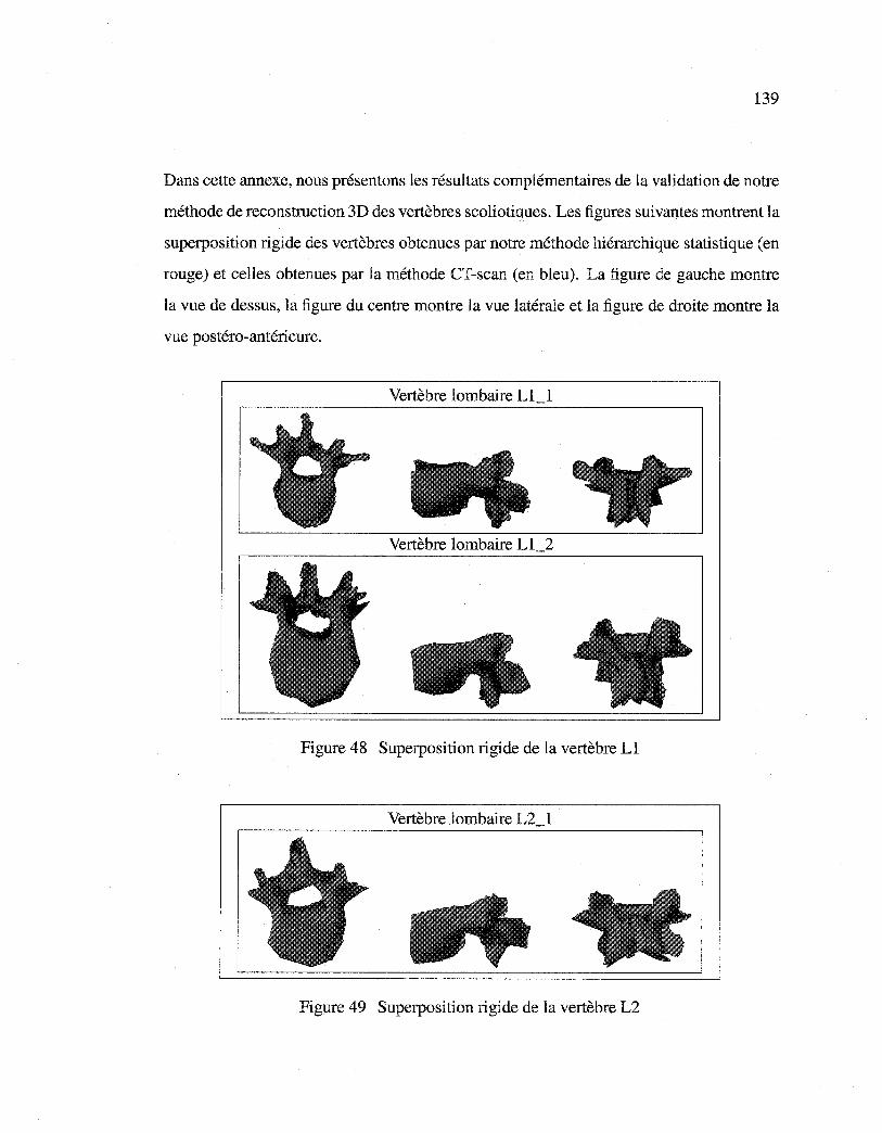
Reproduced with permission of the copyright owner. Further reproduction prohibited without permission.
139
Dans cette annexe, nous présentons les résultats complémentaires de la validation de notre
méthode de reconstruction 3D des vertèbres scoliotiques. Les figures suivantes montrent la
superposition rigide des vertèbres obtenues par notre méthode hiérarchique statistique (en
rouge) et celles obtenues par la méthode CT-scan (en bleu). La figure de gauche montre
la vue de dessus, la figure du centre montre la vue latérale et la figure de droite montre la
vue postéro-antérieure.
Vertèbre lombaire Ll_l
Vertèbre lombaire L1_2
Figure 48 Superposition rigide de la vertèbre Ll
Vertèbre lombaire L2_1
Figure 49 Superposition rigide de la vertèbre L2
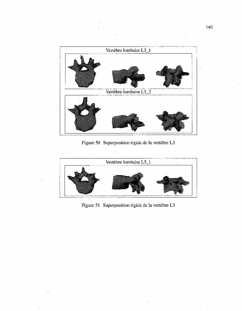
Reproduced with permission of the copyright owner. Further reproduction prohibited without permission.
140
Vertèbre lombaire L3_1
Vertèbre lombaire L3_2
Figure 50 Superposition rigide de la vertèbre L3
Vertèbre lombaire L5_1
Figure 51 Superposition rigide de la vertèbre L5
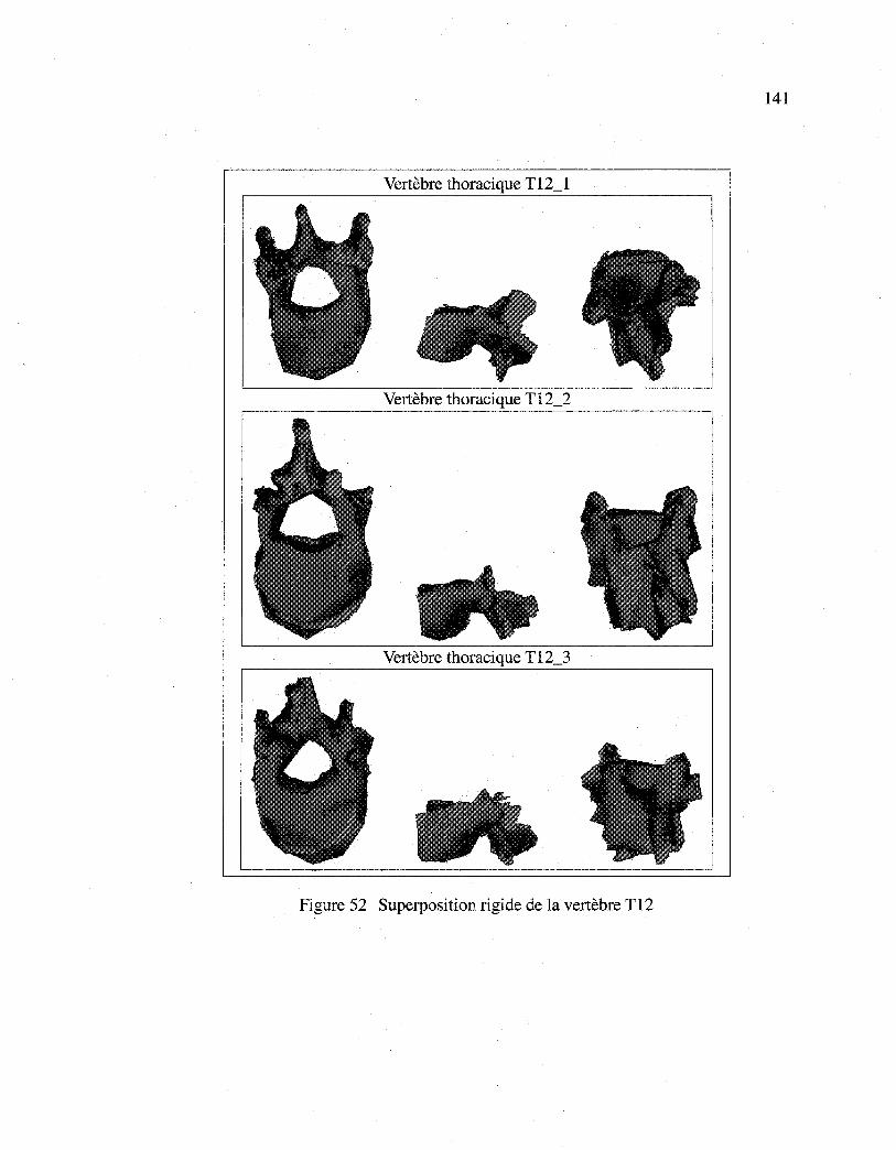
Reproduced with permission of the copyright owner. Further reproduction prohibited without permission.
141
Vertèbre thoracique T12_1
Vertèbre thoracique T12_2
Vertèbre thoracique T12_3
Figure 52 Superposition rigide de la vertèbre T12
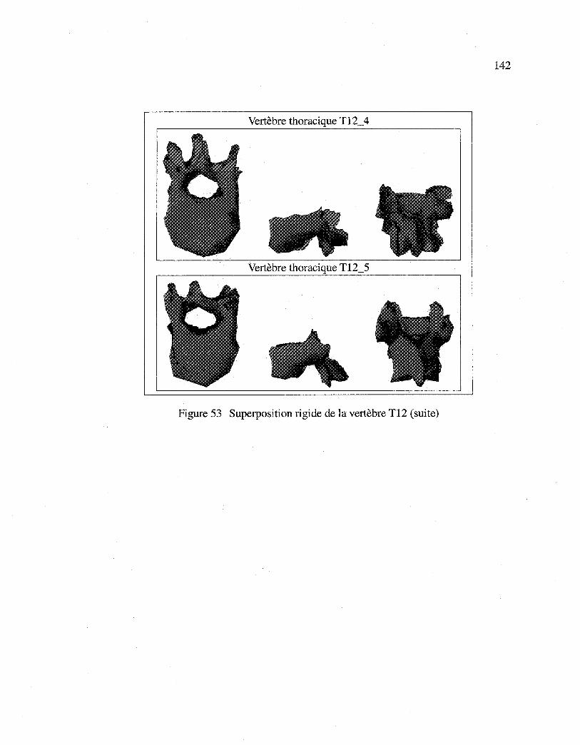
Reproduced with permission of the copyright owner. Further reproduction prohibited without permission.
142
Vertèbre thoracique T12_ 4
Vertèbre thoracique T12_5
Figure 53 Superposition rigide de la vertèbre T12 (suite)
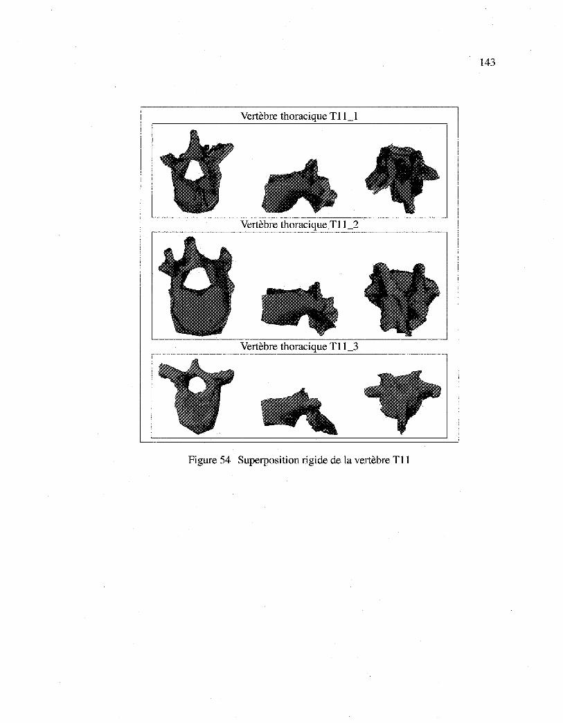
Reproduced with permission of the copyright owner. Further reproduction prohibited without permission.
143
Vertèbre thoracique Tll_l
Vertèbre thoracique Tll_2
Vertèbre thoracique Tll_3
Figure 54 Superposition rigide de la vertèbre Til
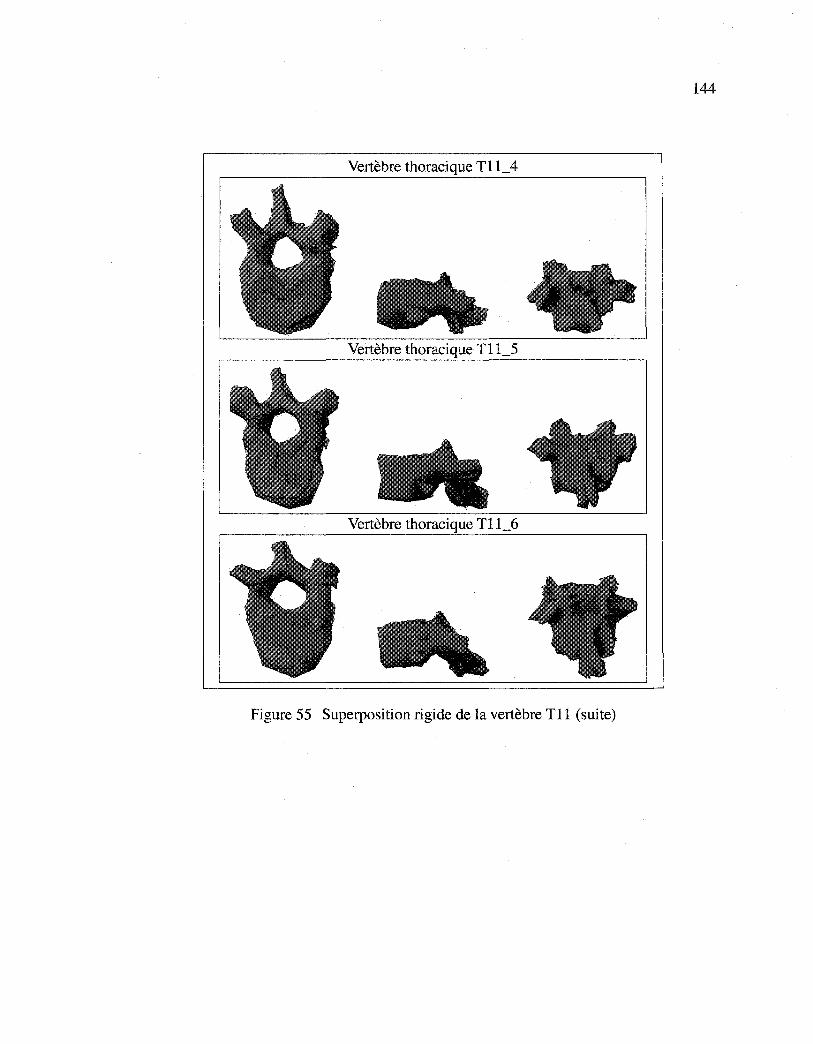
Reproduced with permission of the copyright owner. Further reproduction prohibited without permission.
144
Vertèbre thoracique Tll_ 4
Vertèbre thoracique T11_5
Vertèbre thoracique T11_6
Figure 55 Superposition rigide de la vertèbre Tll (suite)
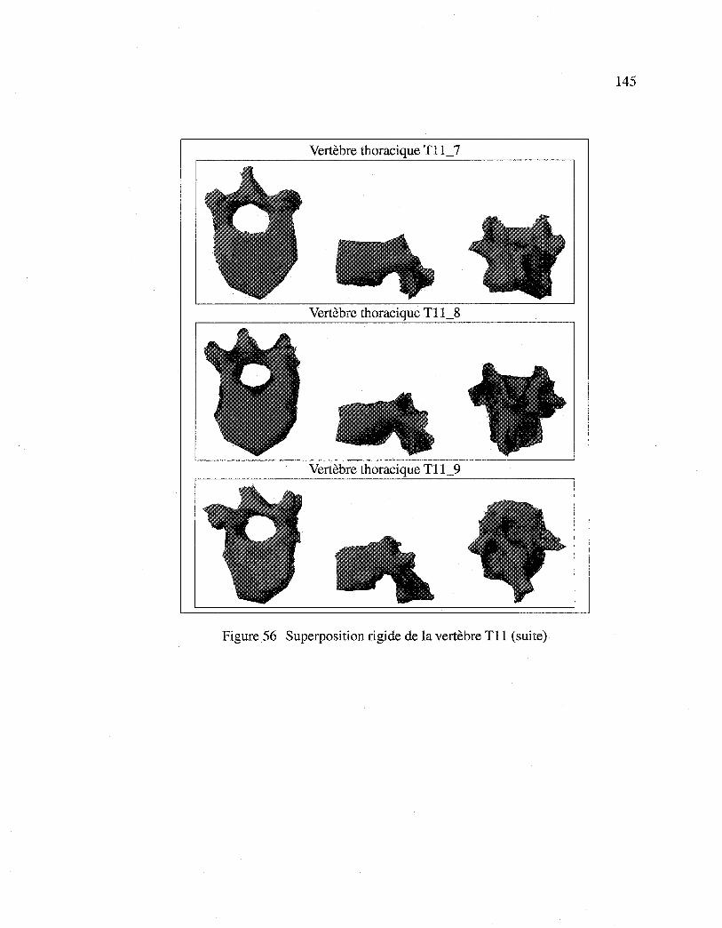
Reproduced with permission of the copyright owner. Further reproduction prohibited without permission.
145
Vertèbre thoracique Tll_7
Vertèbre thoracique Tll_8
Vertèbre thoracique Tll_9
Figure 56 Superposition rigide de la vertèbre Til (suite)
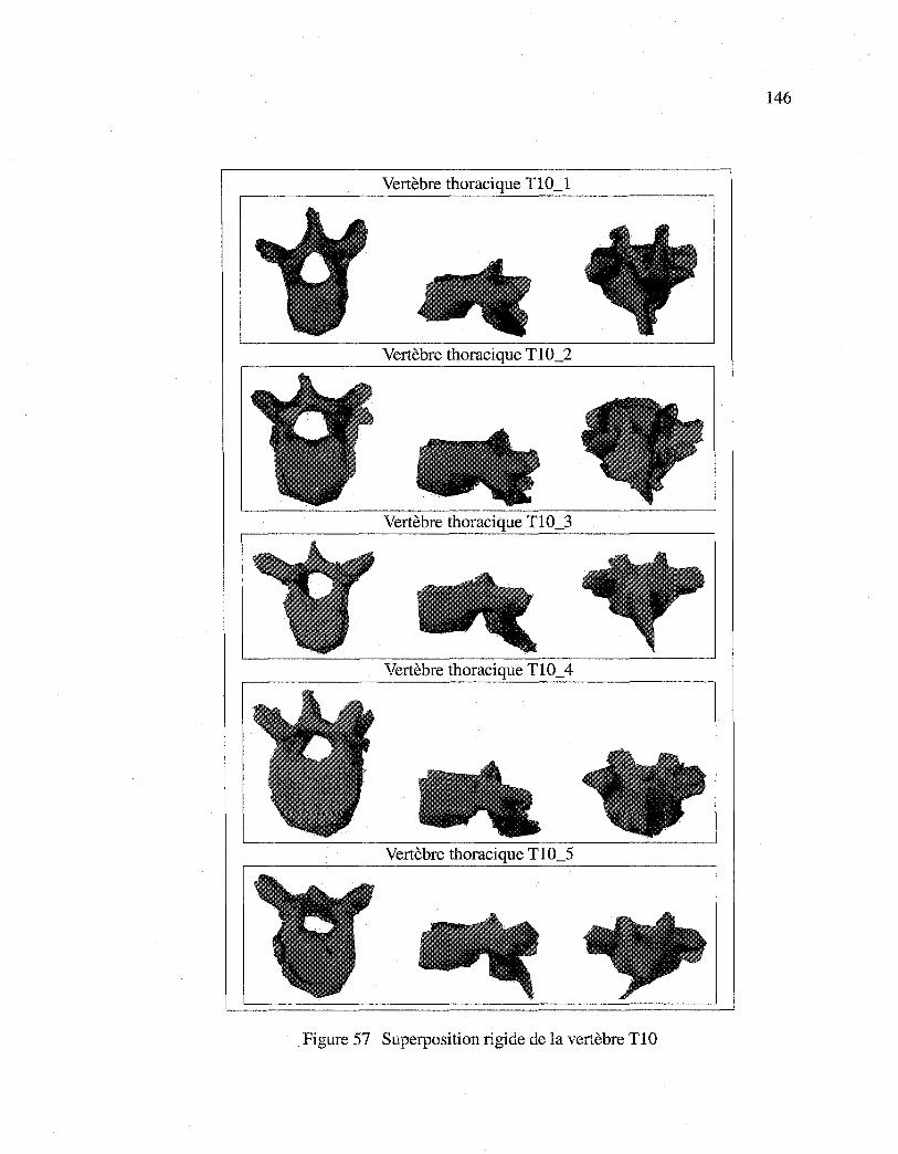
Reproduced with permission of the copyright owner. Further reproduction prohibited without permission.
146
Vertèbre thoracique TlO_l
Vertèbre thoracique Tl0_2
Vertèbre thoracique Tl0_3
Vertèbre thoracique TlO_ 4
Vertèbre thoracique Tl0_5
Figure 57 Superposition rigide de la vertèbre TlO
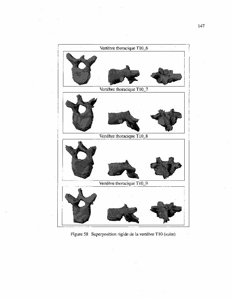
Reproduced with permission of the copyright owner. Further reproduction prohibited without permission.
147
Vertèbre thoracique Tl0_6
Vertèbre thoracique Tl0_7
Vertèbre thoracique Tl0_8
Vertèbre thoracique T10_9
Figure 58 Superposition rigide de la vertèbre TIO (suite)
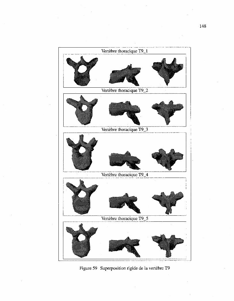
Reproduced with permission of the copyright owner. Further reproduction prohibited without permission.
148
Vertèbre thoracique T9 _1
Vertèbre thoracique T9 _2
Vertèbre thoracique T9 _3
Vertèbre thoracique T9 _ 4
Vertèbre thoracique T9 _5
Figure 59 Superposition rigide de la vertèbre T9
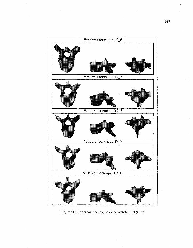
Reproduced with permission of the copyright owner. Further reproduction prohibited without permission.
149
Vertèbre thoracique T9_6
Vertèbre thoracique T9_7
Vertèbre thoracique T9 _8
Vertèbre thoracique T9 _9
Vertèbre thoracique T9 _10
Figure 60 Superposition rigide de la vertèbre T9 (suite)
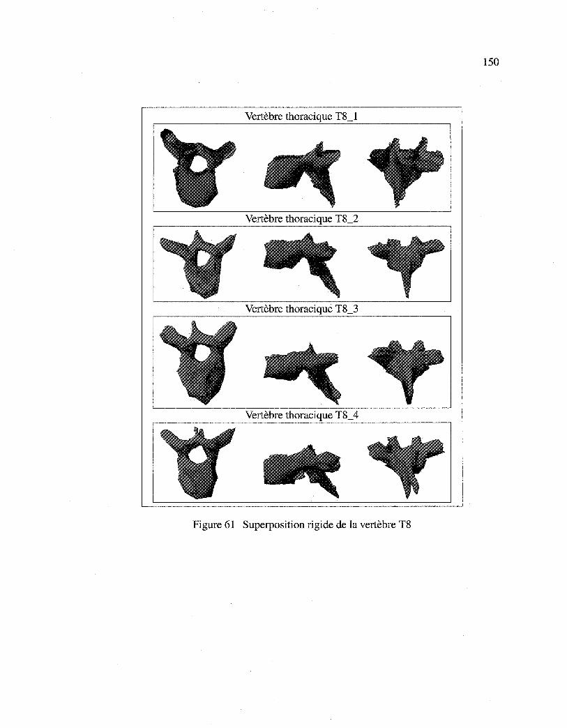
Reproduced with permission of the copyright owner. Further reproduction prohibited without permission.
150
Vertèbre thoracique T8_1
Vertèbre thoracique T8_2
Vertèbre thoracique T8_3
Vertèbre thoracique T8_ 4
Figure 61 Superposition rigide de la vertèbre T8
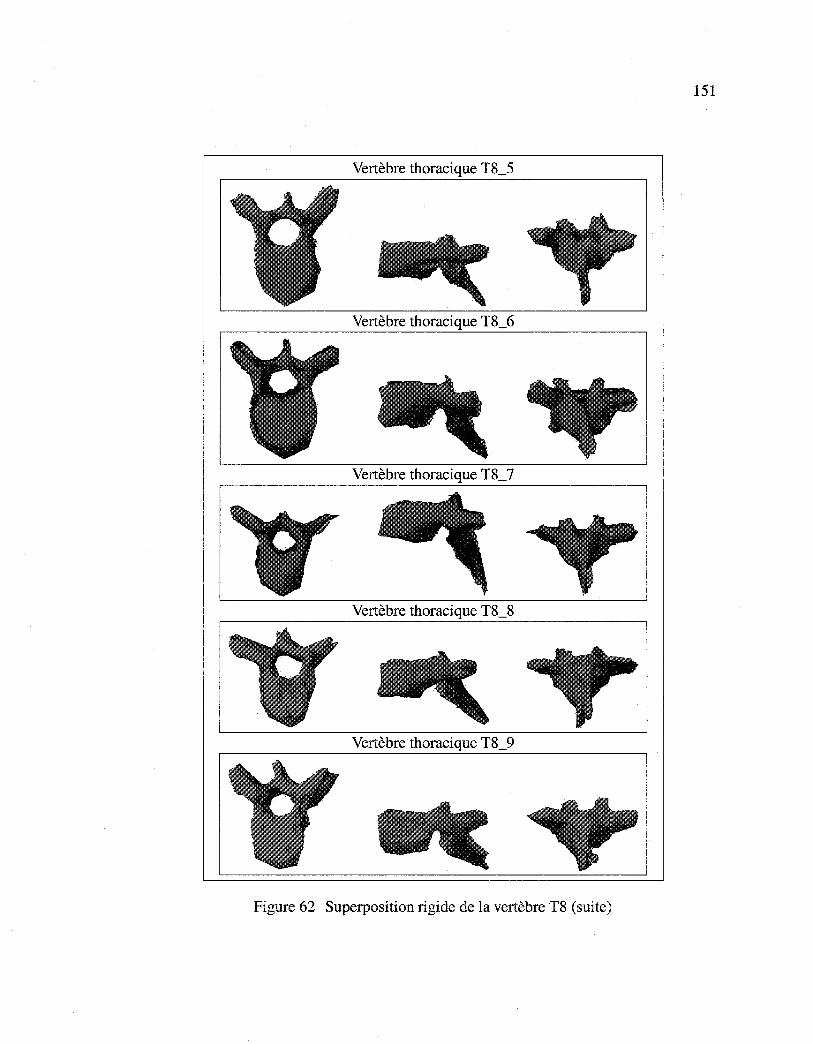
Reproduced with permission of the copyright owner. Further reproduction prohibited without permission.
151
Vertèbre thoracique T8_5
Vertèbre thoracique T8_6
Vertèbre thoracique T8_7
Vertèbre thoracique T8_8
Vertèbre thoracique T8_9
Figure 62 Superposition rigide de la vertèbre T8 (suite)
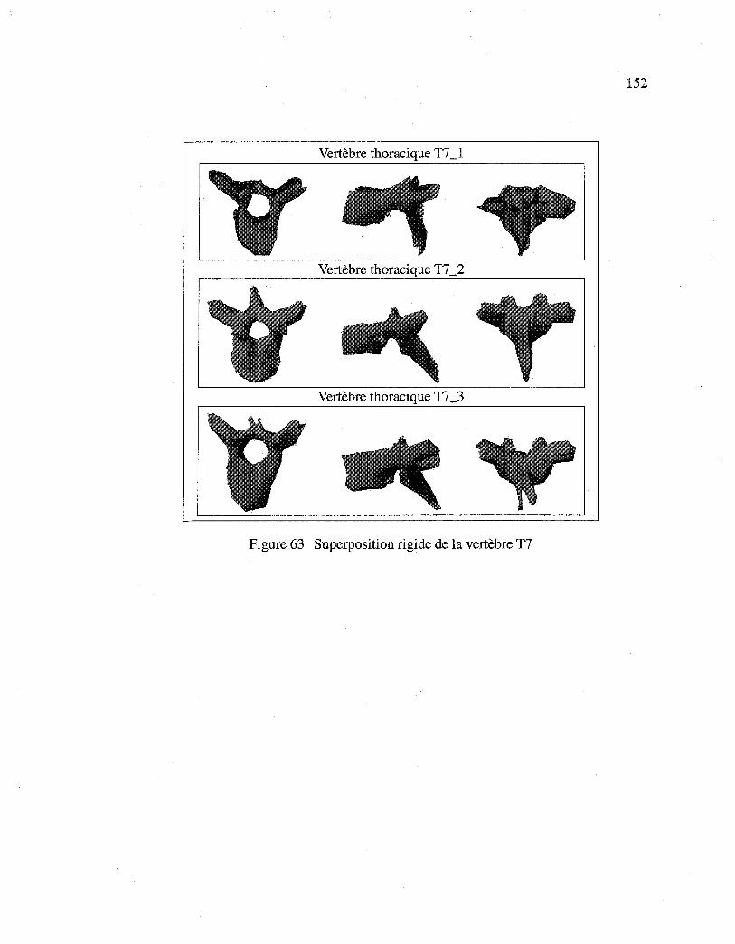
Reproduced with permission of the copyright owner. Further reproduction prohibited without permission.
152
Vertèbre thoracique T7 _1
Vertèbre thoracique T7 _2
Vertèbre thoracique T7 _3
Figure 63 Superposition rigide de la vertèbre T7
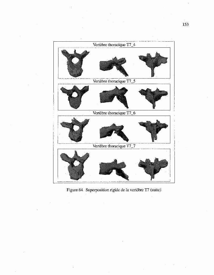
Reproduced with permission of the copyright owner. Further reproduction prohibited without permission.
153
Vertèbre thoracique T7 _ 4
Vertèbre thoracique T7 _5
Vertèbre thoracique T7 _6
Vertèbre thoracique T7 _7
Figure 64 Superposition rigide de la vertèbre T7 (suite)
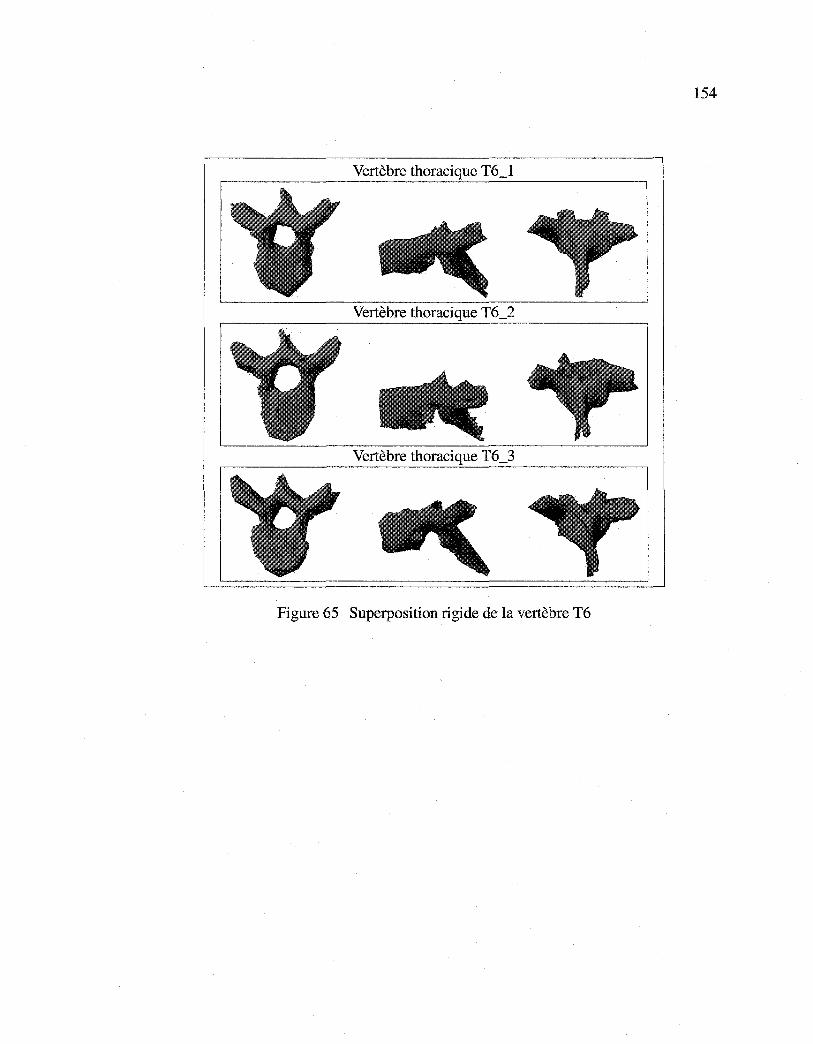
Reproduced with permission of the copyright owner. Further reproduction prohibited without permission.
154
Vertèbre thoracique T6_1
Vertèbre thoracique T6_2
Vertèbre thoracique T6_3
Figure 65 Superposition rigide de la vertèbre T6
Reproduced with permission of the copyright owner. Further reproduction prohibited without permission.
BIBLIOGRAPHIE
[ 1] B. Andre, J. Dansereau, and H. Labelle. Optimized vertical stereo base radiographie setup for the clinical three-dimensional reconstruction of the human spine. Journal of Biomechanics, 27(8): 1023-1035, 1994.
[2] K.S. Arun, T.S. Huang, and S.D. Blostein. Least-square fitting of two 3D point sets. IEEE Transactions on Pattern Analysis and Machine Intelligence, 9(5):698-700, 1987.
[3] C.E. Aubin, J. Dansereau, F. Parent, H. Labelle, and J.A. De Guise. Morphometric evaluations of personalised 3D reconstructions and geometrie models of the human spine. Medical and Biological Engineering and Computing, 35(6):611-618, 1997.
[4] E. Bardinet, L.D. Cohen, and N. Ayache. A parametric deformable model to fit unstructured 3D data. Computer Vision and Image Understanding, 71(1):39-54, 1998.
[5] S. Benameur, M. Mignotte, F. Destrempes, and J.A. De Guise. Estimation of mixture of probabilistic PCA using stochastic EM to the 3D biplanar reconstruction of scoliotic rib cage. In llth IEEE International Conference on Image Processing, Singapore, Octobre 2004, Accepté.
[6] S. Benameur, M. Mignotte, S. Parent, H. Labelle, W. Skalli, and J. De Guise. 3D biplanar reconstruction of scoliotic vertebrae using statistical models. In IEEE Computer Society Conference on Computer Vision and Pattern Recognition, volume 2, pages 577-582, Kauai Marriott, Hawaii, USA, Décembre 2001.
[7] S. Benameur, M. Mignotte, S. Parent, H. Labelle, W. Skalli, and J. De Guise. 3D/2D registration and segmentation of scoliotic vertebrae using statistical models. Computerized Medical Imaging and Graphies, 27(5):321-337, 2003.
[8] S. Benameur, M. Mignotte, S. Parent, H. Labelle, W. Skalli, and J. De Guise. A hierarchical statistical modeling approach for the unsupervised 3D reconstruction of the scoliotic spine. In 1 Oth IEEE International Conference on Image Processing, volume 1, pages 561-564, Barcelona, Spain, Septembre 2003.
[9] R. Benjamin. Object-based 3D X-ray imaging. In Computer Vision, Virtual Reality and Robotics in Medicine, pages 444-448, Paris, France, 1995.
[10] P.J. Besl and N.D. McKay. A method for registration of 3D shapes. IEEE Transactions on Pattern Recognition and Machine Intelligence, 14(2):239-256, 1992.
Reproduced with permission of the copyright owner. Further reproduction prohibited without permission.
156
[11] P.L. Borgne, W. Skalli, I.A.F. Stokes, N. Maurel, G. Beaupère, and F. Lavaste. Three-dimensional measurement of a scoliotic spine. In Three-dimensional analysis of spinal deformities (lOS), pages 219-224. 1995.
[12] L.G. Brown. A survey of image registration techniques. ACM Computing Surveys, 24(4):325-376, 1992.
[13] J.F. Canny. A computational approach to edge detection. IEEE Transactions on Pattern Analysis and Machine Intelligence, 8(6):679-697, 1986.
[14] L. Caponetti and A.M. Fanelli. Computer-aided simulation for bone surgery. IEEE Computer Graphies and Applications, 13(6):86-92, 1993.
[15] V. N. Cassar-Pullicino and S. M. Eisenstein. Imaging in scoliosis: What, why and how? Clinical Radiology, 57(7):543-562, 2002.
[16] C. H. Chien. Reconstruction and recognition of 3D abjects from occluding contours and silhouettes. PhD thesis, Department of Electrical Computer Engineering, University of Texas, Austin, USA, 1987.
[17] T.F. Cootes and C.J.Taylor. A mixture model for representing shape variation. In British Machine Vision Conference, volume 1, pages 110-119, Essex, England, 1997.
[18] T.F. Cootes, D. Cooper, C.J. Taylor, and J. Graham. Active shape models- their training and application. Computer Vision and Image Understanding, 61(1):38-59, 1995.
[19] T.F. Cootes, C.J. Page, C.B. Jackson, and C.J. Taylor. Statistical grey level models for object localization and identication. In British Machine Vision Conference, pages 533-542, 1995.
[20] T.F. Cootes and C.J. Taylor. Active shape models - 'smart snakes'. In British Machine Vision Conferenc, pages 266-275, 1992.
[21] T.F. Cootes and C.J. Taylor. Active shape model search using local grey-level models: a quantitative evaluation. In British Machine Vision Conference, pages 639-648, 1993.
[22] T.F. Cootes, C.J. Taylor, D.H. Cooper, and J. Graham. Training models of shape from sets of examples. In British Machine Vision Conference, pages 9-18, 1992.
[23] T.F. Cootes, C.J. Taylor, and J. Haslam. The use of active shape models for locating structures in medical images. Image and Vision Computing, 12(6):355-365, 1994.
Reproduced with permission of the copyright owner. Further reproduction prohibited without permission.
157
[24] J. Dansereau and I.A.F. Stokes. Measurements of three dimensional shape of the rib cage. Journal ofBiomechanics, 21:893-901, 1988.
[25] C. Davatzikos, X. Tao, and D.Shen. Hierarchical active shape models, using the wavelet transform. IEEE Transactions on Medicalimaging, 22(3):414 -423, 2003.
[26] M. Defontaine, D. Cenonl, L. Colin, C. Yvon, P. Vince, E. Lacaze, R. Dufait, E. Camus, P. Laugier, and F. Patat. A prototype of 500 khz ultrasonic matricial deviee: Bearn scanner. application to in vivo hell bone quantitative characterization. In IEEE International Ultrasonics Symposium, pages 1585-1588, Ceasars Tahoe, Nevada, USA, 1999.
[27] S. Delorme, Y. Petit, J.A. de Guise, C.-E. Aubin, H. Labelle, C. Landry, and J. Dansereau. Three-dimensional modelling and rendering of the human skeletal trunk from 2d radiographie images. In International Conference on 3D Digital Imaging and Modeling, pages 497-505, Ottawa, Canada, Octobre 1999.
[28] S. Delorme, Y. Petit, J.A. de Guise, H. Labelle, C-É. Aubin, and J. Dansereau. Assessment of the 3D reconstruction and high-resolution geometrical modeling of the human skeletal trunk from 2D radiographie images. IEEE Transactions on Biomedical Engineering, 50(8):989-999, 2003.
[29] S. Delorme, P. Violas, J. Dansereau, J.A. de Guise, C.-É. Aubin, and H. Labelle. Preoperative and early postoperative three-dimensional changes of the rib cage after posterior instrumentation in adolescent idiopathie scoliosis. European Spine Journal, 10:101-106, 2000.
[30] P.A. Van den Eisen, J.B.A. Maintz, E.-J.D. Pol, and M.A. Viergever. Medical image matching. a review with classification. IEEE Engineering in Medicine and Biology, 12(1):26-39, 1993.
[31] F. Destrempes. Détection non-supervisée de contours et localisation de formes à l'aide de modèles statistiques. Master's thesis, Department of Computer Science and Operations Research, Université de Montréal, Canada, 2002.
[32] F. Destrempes and M. Mignotte. Unsupervised localization of shapes using statistical models. In International Conference on Signal and Image Processing, pages 60-65, Kauai Marriott, Hawaii, USA, aôut 2002.
[33] J. Diebolt and G. Celeux. Asymptotic properties of a stochastic EM algorithm for estimating mixture proportions. Stochastic Models, 9:599-613, 1993.
Reproduced with permission of the copyright owner. Further reproduction prohibited without permission.
158
[34] M.M. Doody, J.E. Lonstein, M. Stovall, D.G. Hacker, N. Luckyanov, and C.E. Land. Breast cancer mortality after diagnostic radiography: Findings from the u.s. scoliosis cohort study. Spine, 25(16):2052-2063, 2000.
[35] C. Drexler, F. Mattem, and J. Denzler. Hierarchie abject models and classification based on probabilistic PCA. In IAPR Workshop on Machine Vision Applications, pages 435-438, Nara, Japan, Décembre 2002.
[36] M. Dubuisson-Jolly, S. Lakshmanan, and A.K. Jain. Vehicle segmentation and classification using deformable templates. IEEE Transactions on Pattern Analysis and Machine Intelligence, 18(3):293-308, 1996.
[37] J.M. Ferryman, A.D. Worrall, G.D. Sullivan, and K.D. Baker. A generic deformable madel for vehicle recognition. In British Machine Vision Conference, pages 127-136, The University of Birmingham, Birmingham UK, Septembre 1995.
[38] M. Fleute and S. Lavallée. Building a complete surface madel from sparse data using statistical shape models:application to computer assisted knee surgery system. In Medical Image Computing and computer-assisted intervention, pages 879-887. 1998.
[39] M. Fleute and S. Lavallée. Nonrigid 3D/2D registration of images using statistical madel. In Medical Image Computing and Computer-Assisted Intervention, Springer-Verlag, volume 38, pages 138-147. 1999.
[40] B. Godbout, C. Kauffmann, and J.A. de Guise. A simple 2D active contour madel to segment non-convex abjects in 3D images. In Vision Interface, pages 350-358, SFU Harbour Center, Vancouver, British Columbia, Canada, juin 1998.
[41] K. Grauman, G. Shakhnarovich, and T. Darrell. Inferring 3D structure with astatistical image-based shape madel. In IEEE International Conference on Computer Vision, pages 641-648, Nice, France, Octobre 2003.
[42] U. Grenander andD.M. Keenan. Towards automatedimage understanding. Journal of Applied Statistics, 16(2):207-221, 1989.
[43] J.A. De Guise, H. Mallouche, J. Dansereau, and H. Labelle. Imaging techniques applied to spinal biomechanics. Journal of Biomechanics, 7(3):135-144, 1995.
[44] J. Hadamard. Lectures on the Cauchy problem in linear partial differentiai equations. Yale University Press, New Haven, 1923.
[45] J.A. Hartigan and M.A. Wang. A k-means clustering algorithm. Applied Statistics, 28:100-108, 1979.
Reproduced with permission of the copyright owner. Further reproduction prohibited without permission.
159
[46] A. Hill, T.F. Cootes, and C.J. Taylor. A generic system for image interpretation using exible templates. In British Machine Vision Conference, pages 1-10, 1992.
[47] A. Hill, T.F. Cootes, and C.J. Taylor. Active shape models and the shape approximation problem. Image and Vision Computing, 14:601-607, 1996.
[48] A. Hill, T.F. Cootes, C.J. Taylor, and K. Lindley. Medical image interpretation: a generic approach using deformable templates. In Journal Medical Informatics, volume 19, pages 47-59, Janvier- Mars 1994.
[49] A. Hill, A. Thornman, and C.J. Taylor. Model-based interpretation of 3D medical images. In British Machine Vision Conference, pages 339-348, 1993.
[50] B.K.P. Horn. Closed-form solution of absolute orientation using unit quaternions. Journal of the Optical Society of America, 4(4):629-642, 1987.
[51] B.K.P. Horn and N. Shao. Closed-form solution of absolute orientation using orthonormal matrices. Journal of the Optical Society of America, 5(7): 1127-1135, 1988.
[52] T.N. Huynh, J. Dansereau, and G. Maurais. Development of a vertebral endplate 3D reconstruction technique. IEEE Transactions on Medicallmaging, 16(5):689-696, 1997.
[53] A. K. Jain, Y. Zhong, and S. Lakshmanan. Object matching using deformable templates. IEEE Transactions on Pattern Analysis and Machine Intelligence, 18(3):267-278, 1996.
[54] C. Kauffman and J.A. De Guise. Digital radiography segmentation of scoliotic vertebral body using a deformable model. In !nt Soc Optical Engng, volume 3034, pages 243-251, 1997.
[55] C. Kervrann and F. Heitz. A hierarchical statistical framework for the segmentation of deformable objects in image sequences. In IEEE Computer Society Conference on Computer Vision and Pattern Recognition, pages 724-728, Seattle, Washington, USA, Juin 1994.
[56] C. Kervrann and F. Heitz. Statistical deformable model-based segmentation of image motion. IEEE Transactions on Image Processing, 8(4):583-588, 1999.
[57] Y. Kita. Elastic-model driven analysis of several views of a deformable cylindrical object. IEEE Transactions on Pattern Analysis and Machine Intelligence, 18(12):1150-1162, 1996.
Reproduced with permission of the copyright owner. Further reproduction prohibited without permission.
160
[58] J.-M. Laferte, F. Heitz, P. Perez, andE. Fabre. Hierarchical statistical models for the fusion of multiresolution image data. In Fifth International Conference on Computer Vision, pages 908-913, Kauai Marriott, Hawaii, USA, Juin 1995.
[59] S. Lavallée. Computer integrated surgery, chapter Registration for computer integrated surgery: methodology, state of the art, pages 77-97. MIT Press, Cambridge, MA, 1995.
[60] J. Liu and P. Moulin. Image denoising based on scale-space mixture modeling of wavelet coefficients. In IEEE International Conference on Image Processing, pages 386-390, Kobe, Japan, Octobre 1999.
[61] W.E. Lorensen and H.E. Cline. Marching cubes: a high resolution 3D surface construction algorithm. Computer Graphies, 21(4):163-169, 1988.
[62] C. Lorenz and N. Krahnstüver. Generation of point-based 3D statistical shape models for anatomical abjects. Computer Vision and Image Understanding, 77(2): 175-191, 2000.
[63] A. Lorusso, D.W. Eggert, and R.B. Fisher. A comparison of four algorithms for estimating 3D rigid transformations. Machine Vision Applications, 9:272-290, 1997.
[64] J. Lotjonen, I.E. Magnin, J. Nenonen, and T. Katila. Reconstruction of 3D geometry using 2D profiles and a geometrie prior model. IEEE Transactions on Medical Imaging, 18(10):992-1002, 1999.
[65] J. Lotjonen, P-J. Reissman, I.E. Magnin, and T. Katila. Model extraction from magnetic resonance volume data using the deformable pyramid. Medical Image Analysis, 3(4):387-406, 1999.
[66] F. Maes, D. Vandermeulen, and P. Suetens. Comparative evaluation of multiresolution optimization strategies for multimodality image registration by maximization of mutual information. Medical Image Analysis, 3(4):373-386, 1999.
[ 67] J.B .A. Maintz and M.A. Viergever. A survey of medical image registration. Medical Image Analysis, 2(1):1-36, 1998.
[68] J.A. Marchant and C.M. Onyango. Fitting grey level point distribution models to animais in scenes. Image and Vision Computing, 13(1):3-12, 1995.
[69] E. Mareil, J. Dansereau, H. Labelle, and J. De Guise. Incorporation of patient displacement into a trunk reconstruction technique. In Engineering in Medicine and Biology Society. IEEE 17th Annual Conference, volume 1, pages 385 -386, Septembre 1995.
Reproduced with permission of the copyright owner. Further reproduction prohibited without permission.
161
[70] W.N. Martin and J.K. Aggarwal. Volumetrie descriptions of objects from multiple views. IEEE Transactions on Pattern Analysis and Machine Intelligence, 5(2): 150-158, 1983.
[71] G. T. Marzan. Rational design for close-range photogrammetry. PhD thesis, Department of Civil Engineering, University of Illinois at Urbana-Champaign, USA, 1976.
[72] M. Mignotte. Unsupervised statistical sketching for non-photorealistic rendering models. In lOth IEEE International Conference on Image Processing, volume 3, pages 573-577, Barcelona, Spain, Septembre 2003.
[73] M. Mignotte, C. Collet, P. Pérez, and P. Bouthemy. Hybrid genetic optimization and statistical model-based approach for the classification of shadow shapes in sonar imagery. IEEE Transactions on Pattern Analysis and Machine Intelligence, 22(2):129-141, 2000.
[74] M. Mignotte, J. Meunier, and J.-C. Tardif. Endocardial boundary estimation and tracking in echocardiographic images using deformable templates and markov raudom fields. Pattern Analysis and Applications, 4(4):256-271, 2001.
[75] D. Mitton, C. Landry, S. Veron, W. Skalli, F. Lavaste, and J.A. De Guise. 3D reconstruction method from biplanar radiography using non-stereocorresponding points and elastic deformable meshes. Medical and Biological Engineering and Computing, 38(2):133-139, 2000.
[76] A Mitulescu, I. Semaan, J.A. De Guise, P. Leborgne, C. Adamsbaum, and W. Skalli. Validation of the non-stereocorresponding points stereoradiographic 3D reconstruction technique. Medical and Biological Engineering and Computing, 39(2):152-158, 2001.
[77] S. Mouren. Reconstruction 3D biplanaire de cages thoraciques scoliotiques à l'aide de modèles déformables de côtes. Master's thesis, Department of Mechanical Engineering, École Polytechnique at Montréal, Canada, 2003.
[78] B. Nikkhade-Dehkordi, M. Bro-Nielsen, T. Darvann, C. Gramkow, N. Egund, and K. Hermann. 3D reconstruction of the femoral bone using two X-ray images from orthogonal views. In Computer Assisted Radiology, page 1015, Juin 26-29 1996.
[79] F. Olivier. Global optimization with exploration/selection algorithms and simulated annealing. The Annals of Applied Probability, 12:248-271, 2002.
Reproduced with permission of the copyright owner. Further reproduction prohibited without permission.
162
[80] M.M. Panjabi, V. Gael, T. Oxland, K. Takata, J. Duranceau, M. Krag, and M. Priee. Lumbar human vertebrae: quantitative three-dimensional anatomy. Spine, 17(3):299-306, 1992.
[81] M.M. Panjabi, K. Takata, V. Gael, D. Frederico, T. Oxland, J. Duranceau, and M. Krag. Thoracic human vertebrae: quantitative three-dimensional anatomy. Spine, 16(8):888-901, 1991.
[82] S. Parent, H. Labelle, W. Skalli, B. Latimer, and J.A. De Guise. Morphometric analysis of anatomie scoliotic specimens. Spine, 27(21):2305-2311, 2002.
[83] M.J. Pearcy. Stereo radiography of lumbar spine motion. In Acta Orthopaedica Scandinavica Supplementurn, volume 56, pages 7-37, 1985.
[84] C. Pena-Reyes and M. Sipper. Evolutionary computation in medicine: An overview. Artificial Intelligence in Medicine, 19:1-23, 2000.
[85] A. Plamandon, M. Gnon, and G. Maurais. Application of a stereoradiographic method for the study of intervertebral motion. Spine, 13:1027-1032, 1988.
[86] J. Ponce and D. Chelberg. Finding the limbs and cusps of generalized cylinders. International Journal of Computer Vision, 1(3):195-210, 1987.
[87] S. Sandor and R. Leadhy. Surface-based labeling of cortical anatomy using a deformable atlas. IEEE Transactions on Medical Imaging, 16(1):41-54, 1997.
[88] I. Semaan, W. Skalli, S. Veron, A. Templier, J.P. Lasseau, and F. Lavaste. Quantitative three-dimensional anatomy of lumbar spine. European Journal Orthopaedic Surgery, 2001.
[89] I.A.F. Stokes, D.G. Wilder, J.W. Frymoyer, and M.H. Pope. Assessment of patients with low-back pain by biplanar radiographie measurement of intervertebral motion. Spine, 6:233-240, 1981.
[90] D. Terzopoulos, A. Witkin, and M. Kass. Constraints on deformable models: Recovering 3D shape and nonrigidmotion. Artificial Intelligence, 36(1):91-123, 1988.
[91] P. Thévenaz and M. Unser. An efficient mutual information optimizer for multiresolution image registration. In IEEE International Conference on Image Processing, volume 1, pages 833-837, Chicago, 1998.
[92] M.E. Tipping and C.M. Bishop. Mixtures of probabilistic principal component analysers. Neural Computation, 11(2):443-482, 1999.
Reproduced with permission of the copyright owner. Further reproduction prohibited without permission.
163
[93] M.E. Tipping and C.M. Bishop. Probabilistic principal component analysis. Journal of the Royal Statistical Society: Series B, 21(3):611-622, 1999.
[94] F. Trochu. A contouring pro gram based on dual kriging interpolation. Engineering with Computers, 9:160-177, 1993.
[95] H. Veistera and J. Lütjonen. Reconstructing 3D boundary element heart models from 2D biplane fluoroscopy. In T. Katila, I.E. Magnin, P. Clarysse, J. Montagnat, and J. Nenonen, editors, Functionalimaging and Modeling of the Heart, First International Workshop, Helsinki, Finland, volume 2230 of Lecture Notes in Computer Science, pages 17-23. Springer, Novembre 2001.
[96] M. W. Walker, L. Shao, and R.A. Volz. Estimating 3D location parameters using dual number quaternions. CVGIP: Image Understanding, 54(3):358-367, 1991.
[97] J. West. Comparison and evaluation of retrospective inter-modality registration techniques. Computer Assisted Tomography, 1997; http://cswww.vuse.vanderbilt.edu/ image/registration.
[98] G.C. Wiggins, C.I. Shaffrey, M.F. Abel, and A.H. Menezes. Pediatrie spinal deformities. Journal of Neurosurgery and American Association of Neurological Surgeons, 14(1):1-14, 2003.
[99] R.P. Woods, S.T. Grafton, C.J. Holmes, S.R. Cherry, andJ.C. Mazziotta. Automated image registration: I. general methods and intra-subject, intra-modality validation. Journal of Computer Assisted Tomography, 22:141-154, 1998.
[lOO] R.P. Woods, S.T. Grafton, J. Watson, N.L. Sicotte, and J.C. Mazziotta. Automated image registration: ll. intersubject validation of linear and non-linear models. Journal of Computer Assisted Tomography, 22(1): 153-165, 1998.