ÉCOLE DE TECHNOLOGIE SUPÉRIEURE …espace.etsmtl.ca/1570/2/BAUTISTA_Mary_Carmen-web.pdf · La ﬁnesse verticale de la grille de calcul proche des limites du ... Mot-clés: technologíe

ÉCOLE DE TECHNOLOGIE SUPÉRIEURE

UNIVERSITÉ DU QUÉBEC

THESIS PRESENTED TO

ÉCOLE DE TECHNOLOGIE SUPÉRIEURE

IN PARTIAL FULFILLMENT OF THE REQUIREMENTS FOR

THE DEGREE OF

DOCTOR OF PHILOSOPHY

Ph.D.

BY

Mary Carmen BAUTISTA

TURBULENCE MODELLING OF THE ATMOSPHERIC BOUNDARY LAYER OVER

COMPLEX TOPOGRAPHY

MONTREAL, "OCTOBER 19, 2015"

Mary C. Bautista, 2015

This Creative Commons license allows readers to download this work and share it with others as long as the

author is credited. The content of this work cannot be modified in any way or used commercially.

BOARD OF EXAMINERS

THIS THESIS HAS BEEN EVALUATED

BY THE FOLLOWING BOARD OF EXAMINERS:

Prof. Louis Dufresne, Eng., Ph.D., Thesis Advisor

Département de génie mécanique, École de technologie supérieure

Prof. Christian Masson, Eng., Ph.D., Thesis Co-advisor


Prof. François Brissette, Eng., Ph.D., Committee President

Département de génie de la construction, École de technologie supérieure

Prof. Niels N. Sørensen, Eng., Ph.D., External Examiner

Department of Wind Energy, DTU Wind Energy, Technical University of Denmark

Prof. Julien Weiss, Eng., Ph.D., Examiner


THIS THESIS WAS PRESENTED AND DEFENDED

IN THE PRESENCE OF A BOARD OF EXAMINERS AND THE PUBLIC

ON "OCTOBER 5, 2015"

AT ÉCOLE DE TECHNOLOGIE SUPÉRIEURE

ACKNOWLEDGEMENTS

A grateful acknowledgement to my supervisor Prof. Louis Dufresne and co-supervisor

Prof. Christian Masson. Thanks Christian for the financial support and for understanding

straight away the problems behind my questions. Thanks Louis for encouraging me to ask

the right questions. I learned a great deal from your complementary guidance. I also appreci-

ate and thank in advance the thesis evaluation committee for their time, effort and comments.

This research was funded by the Fonds de Recherche du Québec - Nature et Technologies

(FRQ-NT) and the Laboratoire de recherche sur l’Aérodynamique des Éoliennes en milieu

nordique (AEMN). Their support was greatly appreciated.

All the numerical simulations were performed on the Guillimin and Colosse supercomputers

managed by Calcul Québec and Compute Canada. These clusters are maintained by an awe-

some support team. Thank you very much for making many research projects possible. A

special acknowledgement to all the OpenFOAM developers and community for their impor-

tant contributions. In particular to the National Renewable Energy Laboratory (NREL) team

for their outstanding job in the development of the SOWFA package. Matthew Churchfield,

Sang Lee and Pat Moriarty, I am truly grateful for your help and friendship. The time I spend

at NREL was extremely enriching and encouraging. Also thanks to Carlos Peralta because you

always gave me the confidence to ask you questions.

An enormous thanks to all my friends at the ÉTS, in particular to Hugo, Jörn, Pascal and

Louis-Étienne with whom I worked more closely. Thanks for your crucial help over the years

and for being great teachers, but above all thanks for your constant encouragement and great

friendship. To Jon, Simon-Phillipe, Nico, Yann-Aël, Jonathan, Sitraka, Salha, Alex, Joel, Marc,

Hajer, Eric, Nacera, Cherif, Étienne, and Nico, thanks for making my days something worth

remembering. A loving thanks to my family, you are always in my heart. I have come to realize

how much each one of you have positively marked my life. Finally and most important, a huge

thanks to ma petite famille, you are my love, my life and my greatest support. I accomplished

this work and enjoyed these Ph.D. years because of you.

MODÉLISATION DE LA TURBULENCE DANS LA COUCHE LIMITEATMOSPHÉRIQUE SUR TERRAINS COMPLEXES


RÉSUMÉ

De nos jours, l’industrie de l’énergie éolienne emploie différents types de modèle de turbulence

qui sont capables de reproduire correctement et de manière réaliste le comportement de divers

écoulements relativement simples (par ex.: vent au dessus d’un terrain plat, homogène et sans

obstacles). Cependant, l’augmentation de la complexité de l’écoulement (par ex.: dans le

cas de topographies complexes) diminue grandement la précision des modèles de turbulence,

tout en augmentant le coût des calculs. Par conséquent, les simulations précises et fiables des

écoulements au-dessus des terrains complexes demeurent peu pratiques pour les applications

du secteur éolien.

Afin d’améliorer les simulations d’écoulement du vent au-dessus des terrains complexes, deux

des principales difficultés rencontrées dans ce domaine seront présentées dans cette thèse. La

première difficulté est liée au fait que les traitements existants de modèles de surface ne sont

valides que pour les terrains plats. Néanmoins, ces traitements sont fréquemment appliqués à

des simulations d’écoulement au-dessus de terrain complexes. Cependant, le modèle de tur-

bulence k − ω SST (shear stress transport) possède un traitement novateur de la surface qui

le rend moins dépendant des suppositions de terrains plats. La seconde difficulté correspond

aux coûts prohibitifs des simulations lorsque des statistiques précises et fiables sont requises.

Cependant, les modèles hybrides de turbulence peuvent présenter un compromis idéal entre

précision et coût de calculs. Prenant tout cela en compte, les travaux de cette thèse emploient

un modèle de turbulence basé sur le modèle k−ω ainsi que sur la technique hybride dite “sim-

plified improved delayed detached-eddy simulation” (SIDDES), afin d’adresser les besoins du

secteur de l’énergie éolienne.

Pour valider ce modèle d’écoulement atmosphérique, une analyse détaillée d’écoulements typ-

iques est effectuée. Cette validation rigoureuse permet de mieux comprendre les limitations

intrinsèques du modèle de turbulence dans le cadre des calculs numériques effectués. Par la

suite, des simulations de l’écoulement dans la couche atmosphérique neutre au-dessus d’un

terrain plat et homogène sont conduites. Les résultats montrent que le modèle de turbulence

k − ω SST-SIDDES reproduit de manière réaliste le comportement du vent au-dessus de ter-

rains plats et complexes. La finesse verticale de la grille de calcul proche des limites du

domaine requises par ce modèle présente un problème majeur pour la création du maillage.

Cependant, malgré cette limitation, il est démontré dans cette thèse que le modèle de turbulence

k-omega SST-SIDDES représente une approche appropriée à la modélisation de l’écoulement

du vent au-dessus des terrains complexes, et ce, sans avoir à supposer que le terrain est plat et

sans exiger d’importantes ressources de calculs.

VIII

Mot-clés: technologíe eolienne, couche limite atmospheric, modélisation de la turbulence,

model hybride, terrain complexe, simulations microechelle

TURBULENCE MODELLING OF THE ATMOSPHERIC BOUNDARY LAYEROVER COMPLEX TOPOGRAPHY


ABSTRACT

Nowadays, the wind energy industry employs different types of turbulence models which are

capable of reproducing the correct and realistic behaviour of relatively simple flows (e.g. wind

over flat, homogeneous and obstacle free terrain). However, as the complexity of the flow

increases (e.g. wind over complex topography), the accuracy of the turbulence models may

be greatly reduced, and in general, their computational cost rises significantly. Accurate and

reliable flow simulations are still not practical for wind industry applications over complex

terrain.

To improve wind flow simulations over complex terrain, two of the main challenges that the

wind energy sector faces are addressed. The first challenge is related to the fact that ground sur-

face modelling treatments are valid only on flat terrain. Nevertheless, it is a common practice

to use those surface treatments on simulations over complex terrain. However, the k − ω SST

(shear stress transport) turbulence model has a novel surface treatment that is less dependent

on flat terrain assumptions. The second challenge is the high computational cost when accu-

racy and reliable turbulence statistics are needed. Nonetheless hybrid turbulence models could

provide a good compromise between accuracy and computational cost. A turbulence model

based on the k − ω SST model and the simplified improved delayed detached-eddy simulation

(SIDDES) hybrid technique is proposed to address those needs.

To validate this model for atmospheric flows, first an extensive analysis of certain canonical

flows was carried out. This rigorous validation helped understand the inherent limitations of

the turbulence model within the specific numerical framework. Subsequently, computations of

the neutrally stratified atmospheric flow over flat homogeneous terrain and then over complex

topography were conducted. The results show that the k − ω SST-SIDDES turbulence model

is able to predict realistic wind behaviour over flat terrain and more complex cases. The vertical

grid refinement in the near-wall region required by this model poses a major challenge for the

mesh generator. But despite this limitation, k − ω SST-SIDDES turbulence model proved to

be a suitable approach for modelling the wind flow over complex terrain without relying on flat

terrain assumptions or requiring substantial computer resources.

Keywords: wind energy, atmospheric boundary layer, turbulence modelling, hybrid model,

complex topography, microscale simulations

TABLE OF CONTENTS

Page

INTRODUCTION . . . . . . . . . . . . . . . . . . . . . . . . . . . . . . . . . . . . . . . . . . . . . . . . . . . . . . . . . . . . . . . . . . . . . . . . . . . . . . . . 1

CHAPTER 1 THE WIND AND THE ATMOSPHERIC TURBULENT FLOW .. . . . . . . . 7

1.1 Atmospheric boundary layer structure . . . . . . . . . . . . . . . . . . . . . . . . . . . . . . . . . . . . . . . . . . . . . . . . . . 7

1.1.1 Atmospheric surface layer . . . . . . . . . . . . . . . . . . . . . . . . . . . . . . . . . . . . . . . . . . . . . . . . . . . . . 9

1.1.2 Above the atmospheric surface layer . . . . . . . . . . . . . . . . . . . . . . . . . . . . . . . . . . . . . . . . 12

1.2 Effects over complex topography . . . . . . . . . . . . . . . . . . . . . . . . . . . . . . . . . . . . . . . . . . . . . . . . . . . . . . 13

1.2.1 Turbine micro-siting . . . . . . . . . . . . . . . . . . . . . . . . . . . . . . . . . . . . . . . . . . . . . . . . . . . . . . . . . . 16

1.3 Turbulence . . . . . . . . . . . . . . . . . . . . . . . . . . . . . . . . . . . . . . . . . . . . . . . . . . . . . . . . . . . . . . . . . . . . . . . . . . . . . . . 17

1.4 Microscale flow governing equations . . . . . . . . . . . . . . . . . . . . . . . . . . . . . . . . . . . . . . . . . . . . . . . . . . 19

CHAPTER 2 MICROSCALE ATMOSPHERIC FLOW MODELLING . . . . . . . . . . . . . . . . . 21

2.1 Basics aspects of computational fluid dynamics . . . . . . . . . . . . . . . . . . . . . . . . . . . . . . . . . . . . . . . 21

2.1.1 Physical modelling . . . . . . . . . . . . . . . . . . . . . . . . . . . . . . . . . . . . . . . . . . . . . . . . . . . . . . . . . . . . 22

2.1.2 Numerical techniques in OpenFOAM .. . . . . . . . . . . . . . . . . . . . . . . . . . . . . . . . . . . . . . 29

2.1.3 Additional details of the OpenFOAM framework . . . . . . . . . . . . . . . . . . . . . . . . . . . 32

2.2 Challenges in microscale wind energy simulations . . . . . . . . . . . . . . . . . . . . . . . . . . . . . . . . . . . . 33

2.2.1 Proposed hybrid model for atmospheric flow simulations . . . . . . . . . . . . . . . . . . 34

2.2.1.1 Roughness extension and meshing . . . . . . . . . . . . . . . . . . . . . . . . . . . . . . . 39

2.3 Summary and subsequent tasks . . . . . . . . . . . . . . . . . . . . . . . . . . . . . . . . . . . . . . . . . . . . . . . . . . . . . . . . . 43

CHAPTER 3 TURBULENCE MODEL VALIDATION ON CANONICAL

FLOWS . . . . . . . . . . . . . . . . . . . . . . . . . . . . . . . . . . . . . . . . . . . . . . . . . . . . . . . . . . . . . . . . . . . . . . . 45

3.1 Decaying isotropic turbulence flow . . . . . . . . . . . . . . . . . . . . . . . . . . . . . . . . . . . . . . . . . . . . . . . . . . . . 45

3.2 Decaying turbulence with rotation effects . . . . . . . . . . . . . . . . . . . . . . . . . . . . . . . . . . . . . . . . . . . . . 55

3.3 Free homogeneous shear turbulence . . . . . . . . . . . . . . . . . . . . . . . . . . . . . . . . . . . . . . . . . . . . . . . . . . . 62

3.4 Channel flow . . . . . . . . . . . . . . . . . . . . . . . . . . . . . . . . . . . . . . . . . . . . . . . . . . . . . . . . . . . . . . . . . . . . . . . . . . . . 70

3.5 Summary . . . . . . . . . . . . . . . . . . . . . . . . . . . . . . . . . . . . . . . . . . . . . . . . . . . . . . . . . . . . . . . . . . . . . . . . . . . . . . . . 76

CHAPTER 4 MICROSCALE ATMOSPHERIC FLOW SIMULATIONS

OVER FLAT TOPOGRAPHY . . . . . . . . . . . . . . . . . . . . . . . . . . . . . . . . . . . . . . . . . . . . . . 79

4.1 Atmospheric surface layer . . . . . . . . . . . . . . . . . . . . . . . . . . . . . . . . . . . . . . . . . . . . . . . . . . . . . . . . . . . . . 80

4.2 Idealized neutral atmospheric boundary layer . . . . . . . . . . . . . . . . . . . . . . . . . . . . . . . . . . . . . . . . . 84

4.2.1 Pressure driven atmospheric flow . . . . . . . . . . . . . . . . . . . . . . . . . . . . . . . . . . . . . . . . . . . . 84

4.2.2 Pressure driven atmospheric flow with Coriolis force . . . . . . . . . . . . . . . . . . . . . .100

4.3 Høvsøre field measurement campaign: neutral case . . . . . . . . . . . . . . . . . . . . . . . . . . . . . . . . . .105

4.4 Summary . . . . . . . . . . . . . . . . . . . . . . . . . . . . . . . . . . . . . . . . . . . . . . . . . . . . . . . . . . . . . . . . . . . . . . . . . . . . . . .107

XII

CHAPTER 5 MICROSCALE ATMOSPHERIC FLOW SIMULATIONS

OVER COMPLEX TOPOGRAPHY . . . . . . . . . . . . . . . . . . . . . . . . . . . . . . . . . . . . . . .109

5.1 Flow around a square-section cylinder . . . . . . . . . . . . . . . . . . . . . . . . . . . . . . . . . . . . . . . . . . . . . . . .110

5.1.1 Case A: Approaching thin boundary layer flow . . . . . . . . . . . . . . . . . . . . . . . . . . .114

5.1.2 Case B: Approaching thick boundary layer flow . . . . . . . . . . . . . . . . . . . . . . . . . . .126

5.1.2.1 Case B1: Imposed inlet profiles . . . . . . . . . . . . . . . . . . . . . . . . . . . . . . . . .127

5.1.2.2 Case B2: Imposed inlet profiles with ABL constants . . . . . . . . . .131

5.1.2.3 Case B3: Mapped inlet from a precursor simulation . . . . . . . . . . .133

5.1.3 Overview . . . . . . . . . . . . . . . . . . . . . . . . . . . . . . . . . . . . . . . . . . . . . . . . . . . . . . . . . . . . . . . . . . . . .140

5.2 Askervein hill measurement campaign . . . . . . . . . . . . . . . . . . . . . . . . . . . . . . . . . . . . . . . . . . . . . . . .142

5.2.1 Overview . . . . . . . . . . . . . . . . . . . . . . . . . . . . . . . . . . . . . . . . . . . . . . . . . . . . . . . . . . . . . . . . . . . . .151

CONCLUSION . . . . . . . . . . . . . . . . . . . . . . . . . . . . . . . . . . . . . . . . . . . . . . . . . . . . . . . . . . . . . . . . . . . . . . . . . . . . . . . . .155

APPENDIX I k − ω SST-SIDDES HYBRID MODEL EQUATIONS . . . . . . . . . . . . . . . . . . .159

APPENDIX II FORMULATION OF THE DES, DDES AND IDDES MODELS . . . . . . .163

APPENDIX III OPENFOAM CODE . . . . . . . . . . . . . . . . . . . . . . . . . . . . . . . . . . . . . . . . . . . . . . . . . . . . . . . .167

BIBLIOGRAPHY . . . . . . . . . . . . . . . . . . . . . . . . . . . . . . . . . . . . . . . . . . . . . . . . . . . . . . . . . . . . . . . . . . . . . . . . . . . . . .179

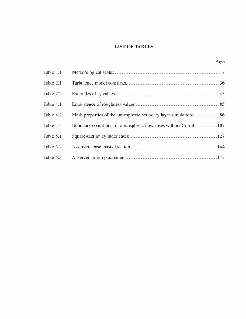
LIST OF TABLES

Page

Table 1.1 Meteorological scales . . . . . . . . . . . . . . . . . . . . . . . . . . . . . . . . . . . . . . . . . . . . . . . . . . . . . . . . . . . . . 7

Table 2.1 Turbulence model constants. . . . . . . . . . . . . . . . . . . . . . . . . . . . . . . . . . . . . . . . . . . . . . . . . . . . . 36

Table 2.2 Examples of z1 values . . . . . . . . . . . . . . . . . . . . . . . . . . . . . . . . . . . . . . . . . . . . . . . . . . . . . . . . . . . 43

Table 4.1 Equivalence of roughness values . . . . . . . . . . . . . . . . . . . . . . . . . . . . . . . . . . . . . . . . . . . . . . . . 85

Table 4.2 Mesh properties of the atmospheric boundary layer simulations . . . . . . . . . . . . . . 86

Table 4.3 Boundary conditions for atmospheric flow cases without Coriolis . . . . . . . . . . .107

Table 5.1 Square-section cylinder cases . . . . . . . . . . . . . . . . . . . . . . . . . . . . . . . . . . . . . . . . . . . . . . . . . .127

Table 5.2 Askervein case masts location . . . . . . . . . . . . . . . . . . . . . . . . . . . . . . . . . . . . . . . . . . . . . . . . . .144

Table 5.3 Askervein mesh parameters . . . . . . . . . . . . . . . . . . . . . . . . . . . . . . . . . . . . . . . . . . . . . . . . . . . .147

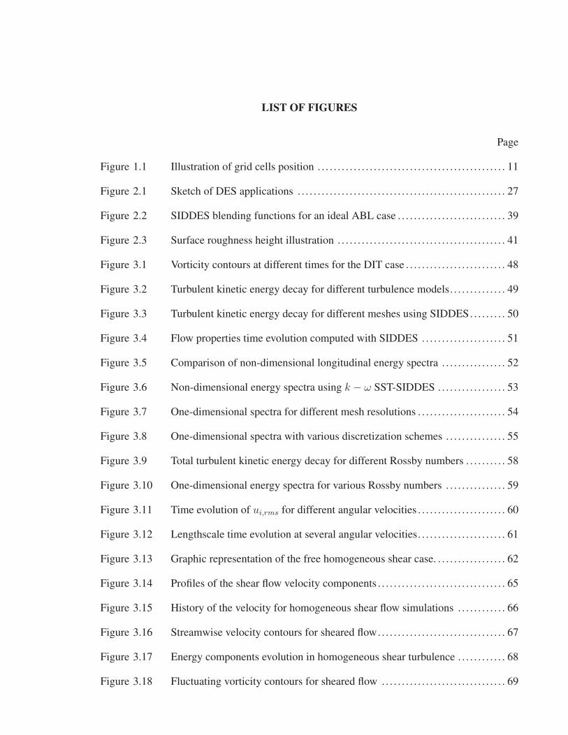
LIST OF FIGURES

Page

Figure 1.1 Illustration of grid cells position . . . . . . . . . . . . . . . . . . . . . . . . . . . . . . . . . . . . . . . . . . . . . . . 11

Figure 2.1 Sketch of DES applications . . . . . . . . . . . . . . . . . . . . . . . . . . . . . . . . . . . . . . . . . . . . . . . . . . . . 27

Figure 2.2 SIDDES blending functions for an ideal ABL case . . . . . . . . . . . . . . . . . . . . . . . . . . . 39

Figure 2.3 Surface roughness height illustration . . . . . . . . . . . . . . . . . . . . . . . . . . . . . . . . . . . . . . . . . . 41

Figure 3.1 Vorticity contours at different times for the DIT case . . . . . . . . . . . . . . . . . . . . . . . . . 48

Figure 3.2 Turbulent kinetic energy decay for different turbulence models. . . . . . . . . . . . . . 49

Figure 3.3 Turbulent kinetic energy decay for different meshes using SIDDES. . . . . . . . . 50

Figure 3.4 Flow properties time evolution computed with SIDDES . . . . . . . . . . . . . . . . . . . . . 51

Figure 3.5 Comparison of non-dimensional longitudinal energy spectra . . . . . . . . . . . . . . . . 52

Figure 3.6 Non-dimensional energy spectra using k − ω SST-SIDDES . . . . . . . . . . . . . . . . . 53

Figure 3.7 One-dimensional spectra for different mesh resolutions . . . . . . . . . . . . . . . . . . . . . . 54

Figure 3.8 One-dimensional spectra with various discretization schemes . . . . . . . . . . . . . . . 55

Figure 3.9 Total turbulent kinetic energy decay for different Rossby numbers . . . . . . . . . . 58

Figure 3.10 One-dimensional energy spectra for various Rossby numbers . . . . . . . . . . . . . . . 59

Figure 3.11 Time evolution of ui,rms for different angular velocities . . . . . . . . . . . . . . . . . . . . . . 60

Figure 3.12 Lengthscale time evolution at several angular velocities. . . . . . . . . . . . . . . . . . . . . . 61

Figure 3.13 Graphic representation of the free homogeneous shear case. . . . . . . . . . . . . . . . . . 62

Figure 3.14 Profiles of the shear flow velocity components . . . . . . . . . . . . . . . . . . . . . . . . . . . . . . . . 65

Figure 3.15 History of the velocity for homogeneous shear flow simulations . . . . . . . . . . . . 66

Figure 3.16 Streamwise velocity contours for sheared flow. . . . . . . . . . . . . . . . . . . . . . . . . . . . . . . . 67

Figure 3.17 Energy components evolution in homogeneous shear turbulence . . . . . . . . . . . . 68

Figure 3.18 Fluctuating vorticity contours for sheared flow . . . . . . . . . . . . . . . . . . . . . . . . . . . . . . . 69

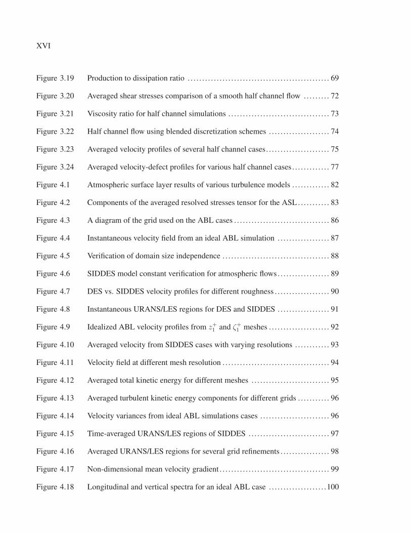
XVI

Figure 3.19 Production to dissipation ratio . . . . . . . . . . . . . . . . . . . . . . . . . . . . . . . . . . . . . . . . . . . . . . . . . 69

Figure 3.20 Averaged shear stresses comparison of a smooth half channel flow . . . . . . . . . 72

Figure 3.21 Viscosity ratio for half channel simulations . . . . . . . . . . . . . . . . . . . . . . . . . . . . . . . . . . . 73

Figure 3.22 Half channel flow using blended discretization schemes . . . . . . . . . . . . . . . . . . . . . 74

Figure 3.23 Averaged velocity profiles of several half channel cases. . . . . . . . . . . . . . . . . . . . . . 75

Figure 3.24 Averaged velocity-defect profiles for various half channel cases. . . . . . . . . . . . . 77

Figure 4.1 Atmospheric surface layer results of various turbulence models . . . . . . . . . . . . . 82

Figure 4.2 Components of the averaged resolved stresses tensor for the ASL . . . . . . . . . . . 83

Figure 4.3 A diagram of the grid used on the ABL cases . . . . . . . . . . . . . . . . . . . . . . . . . . . . . . . . . 86

Figure 4.4 Instantaneous velocity field from an ideal ABL simulation . . . . . . . . . . . . . . . . . . 87

Figure 4.5 Verification of domain size independence . . . . . . . . . . . . . . . . . . . . . . . . . . . . . . . . . . . . . 88

Figure 4.6 SIDDES model constant verification for atmospheric flows . . . . . . . . . . . . . . . . . . 89

Figure 4.7 DES vs. SIDDES velocity profiles for different roughness . . . . . . . . . . . . . . . . . . . 90

Figure 4.8 Instantaneous URANS/LES regions for DES and SIDDES . . . . . . . . . . . . . . . . . . 91

Figure 4.9 Idealized ABL velocity profiles from z+1 and ζ+1 meshes . . . . . . . . . . . . . . . . . . . . . 92

Figure 4.10 Averaged velocity from SIDDES cases with varying resolutions . . . . . . . . . . . . 93

Figure 4.11 Velocity field at different mesh resolution . . . . . . . . . . . . . . . . . . . . . . . . . . . . . . . . . . . . . 94

Figure 4.12 Averaged total kinetic energy for different meshes . . . . . . . . . . . . . . . . . . . . . . . . . . . 95

Figure 4.13 Averaged turbulent kinetic energy components for different grids . . . . . . . . . . . 96

Figure 4.14 Velocity variances from ideal ABL simulations cases . . . . . . . . . . . . . . . . . . . . . . . . 96

Figure 4.15 Time-averaged URANS/LES regions of SIDDES . . . . . . . . . . . . . . . . . . . . . . . . . . . . 97

Figure 4.16 Averaged URANS/LES regions for several grid refinements . . . . . . . . . . . . . . . . . 98

Figure 4.17 Non-dimensional mean velocity gradient . . . . . . . . . . . . . . . . . . . . . . . . . . . . . . . . . . . . . . 99

Figure 4.18 Longitudinal and vertical spectra for an ideal ABL case . . . . . . . . . . . . . . . . . . . .100

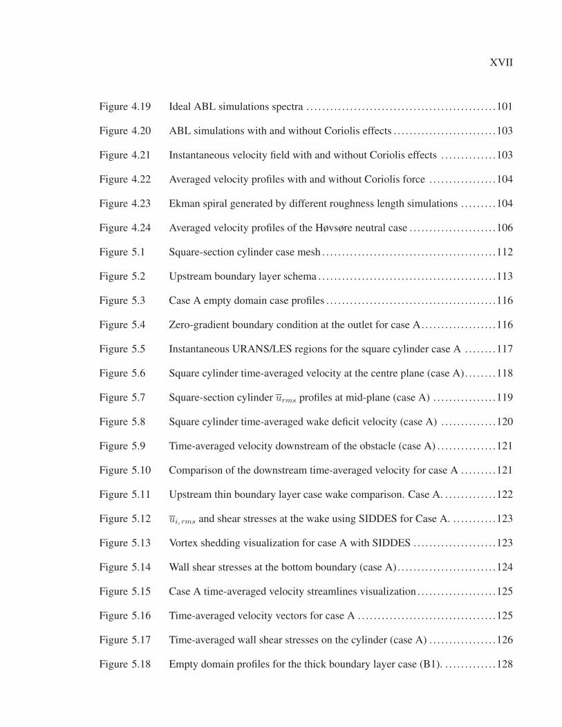
XVII

Figure 4.19 Ideal ABL simulations spectra . . . . . . . . . . . . . . . . . . . . . . . . . . . . . . . . . . . . . . . . . . . . . . . .101

Figure 4.20 ABL simulations with and without Coriolis effects . . . . . . . . . . . . . . . . . . . . . . . . . .103

Figure 4.21 Instantaneous velocity field with and without Coriolis effects . . . . . . . . . . . . . .103

Figure 4.22 Averaged velocity profiles with and without Coriolis force . . . . . . . . . . . . . . . . .104

Figure 4.23 Ekman spiral generated by different roughness length simulations . . . . . . . . .104

Figure 4.24 Averaged velocity profiles of the Høvsøre neutral case . . . . . . . . . . . . . . . . . . . . . .106

Figure 5.1 Square-section cylinder case mesh . . . . . . . . . . . . . . . . . . . . . . . . . . . . . . . . . . . . . . . . . . . .112

Figure 5.2 Upstream boundary layer schema . . . . . . . . . . . . . . . . . . . . . . . . . . . . . . . . . . . . . . . . . . . . .113

Figure 5.3 Case A empty domain case profiles . . . . . . . . . . . . . . . . . . . . . . . . . . . . . . . . . . . . . . . . . . .116

Figure 5.4 Zero-gradient boundary condition at the outlet for case A. . . . . . . . . . . . . . . . . . .116

Figure 5.5 Instantaneous URANS/LES regions for the square cylinder case A . . . . . . . .117

Figure 5.6 Square cylinder time-averaged velocity at the centre plane (case A). . . . . . . .118

Figure 5.7 Square-section cylinder urms profiles at mid-plane (case A) . . . . . . . . . . . . . . . .119

Figure 5.8 Square cylinder time-averaged wake deficit velocity (case A) . . . . . . . . . . . . . .120

Figure 5.9 Time-averaged velocity downstream of the obstacle (case A) . . . . . . . . . . . . . . .121

Figure 5.10 Comparison of the downstream time-averaged velocity for case A . . . . . . . . .121

Figure 5.11 Upstream thin boundary layer case wake comparison. Case A. . . . . . . . . . . . . .122

Figure 5.12 ui, rms and shear stresses at the wake using SIDDES for Case A. . . . . . . . . . . .123

Figure 5.13 Vortex shedding visualization for case A with SIDDES . . . . . . . . . . . . . . . . . . . . .123

Figure 5.14 Wall shear stresses at the bottom boundary (case A). . . . . . . . . . . . . . . . . . . . . . . . .124

Figure 5.15 Case A time-averaged velocity streamlines visualization . . . . . . . . . . . . . . . . . . . .125

Figure 5.16 Time-averaged velocity vectors for case A . . . . . . . . . . . . . . . . . . . . . . . . . . . . . . . . . . .125

Figure 5.17 Time-averaged wall shear stresses on the cylinder (case A) . . . . . . . . . . . . . . . . .126

Figure 5.18 Empty domain profiles for the thick boundary layer case (B1). . . . . . . . . . . . . .128

XVIII

Figure 5.19 URANS/LES regions of the immersed cylinder case B1 . . . . . . . . . . . . . . . . . . . .128

Figure 5.20 Wake velocity deficit for the thick boundary layer case B1. . . . . . . . . . . . . . . . . .129

Figure 5.21 Downstream velocity on the thick boundary layer case B1 . . . . . . . . . . . . . . . . . .130

Figure 5.22 Case A and B1 profiles comparison. . . . . . . . . . . . . . . . . . . . . . . . . . . . . . . . . . . . . . . . . . .130

Figure 5.23 Mean URANS/LES regions for case B2 . . . . . . . . . . . . . . . . . . . . . . . . . . . . . . . . . . . . . .132

Figure 5.24 Case B1 and B2 profiles comparison . . . . . . . . . . . . . . . . . . . . . . . . . . . . . . . . . . . . . . . . .132

Figure 5.25 Wake velocity deficit for the thick boundary layer cases B1 and B2 . . . . . . . .133

Figure 5.26 Downstream velocity for the thick boundary layer cases B1 and B2. . . . . . . .134

Figure 5.27 Schema of case B3 . . . . . . . . . . . . . . . . . . . . . . . . . . . . . . . . . . . . . . . . . . . . . . . . . . . . . . . . . . . . .135

Figure 5.28 Profiles of the empty domain thick boundary layer cases B2 and B3 . . . . . . .135

Figure 5.29 Time-averaged URANS/LES regions (case B3). . . . . . . . . . . . . . . . . . . . . . . . . . . . . .136

Figure 5.30 Downstream time-averaged velocity for case B3. . . . . . . . . . . . . . . . . . . . . . . . . . . . .137

Figure 5.31 ui, rms and shear stresses for case B3 at x = 5d . . . . . . . . . . . . . . . . . . . . . . . . . . . . . .137

Figure 5.32 Case B3 time-averaged velocity streamlines visualization . . . . . . . . . . . . . . . . . .138

Figure 5.33 Time-averaged velocity vectors (Case B3) . . . . . . . . . . . . . . . . . . . . . . . . . . . . . . . . . . .138

Figure 5.34 Time-averaged wall shear stresses on the cylinder in case B3 . . . . . . . . . . . . . . .139

Figure 5.35 Case B3 time-averaged wall shear stresses at the bottom boundary. . . . . . . . .140

Figure 5.36 Wall shear stresses for the square-section cylinder cases A and B3 . . . . . . . . .141

Figure 5.37 Velocity and turbulence intensity comparison of cases A and B3 . . . . . . . . . . .141

Figure 5.38 Picture of the Askervein hill . . . . . . . . . . . . . . . . . . . . . . . . . . . . . . . . . . . . . . . . . . . . . . . . . . .143

Figure 5.39 Askervein contour map and reference points location . . . . . . . . . . . . . . . . . . . . . . .143

Figure 5.40 Askervein simulation domain . . . . . . . . . . . . . . . . . . . . . . . . . . . . . . . . . . . . . . . . . . . . . . . . .146

Figure 5.41 Askervein case mesh. . . . . . . . . . . . . . . . . . . . . . . . . . . . . . . . . . . . . . . . . . . . . . . . . . . . . . . . . . .147

Figure 5.42 URANS/LES regions in the Askervein hill case . . . . . . . . . . . . . . . . . . . . . . . . . . . . .148

XIX

Figure 5.43 Time-averaged vertical profiles at the reference point RS . . . . . . . . . . . . . . . . . . .149

Figure 5.44 Time-averaged velocity profiles at RS and HT . . . . . . . . . . . . . . . . . . . . . . . . . . . . . . .150

Figure 5.45 Total turbulent kinetic energy at RS and HT . . . . . . . . . . . . . . . . . . . . . . . . . . . . . . . . .150

Figure 5.46 Vertical speed-up ratio at HT . . . . . . . . . . . . . . . . . . . . . . . . . . . . . . . . . . . . . . . . . . . . . . . . . .151

Figure 5.47 Speed-up across the Askervein hill at z = 10 m .. . . . . . . . . . . . . . . . . . . . . . . . . . . .152

Figure 5.48 Turbulent kinetic energy across the Askervein hill at z = 10 m .. . . . . . . . . . . .152

Figure 5.49 Mesh A velocity field at z = 10 m .. . . . . . . . . . . . . . . . . . . . . . . . . . . . . . . . . . . . . . . . . . .153

LIST OF ABREVIATIONS

ABL atmospheric boundary layer

AGL above ground level

ASL atmospheric surface layer

BL boundary layer

CDS central difference scheme

CFD computational fluid dynamics

CFL Courant–Friedrichs–Lewy stability condition

DES detached-eddy simulation

DIT decaying isotropic turbulence

DDES delayed detached-eddy simulation

DNS direct numerical simulation

FDS filteredLinear discretization scheme

FVM finite volume method

GIS grid induced separation

HAT homogeneous anisotropic turbulence

HSF homogeneous shear flow

IDDES improved delayed detached-eddy simulation

LES large-eddy simulation

LLM logarithmic layer mismatch

XXII

OpenFOAM open source field operation and manipulation software

PISO pressure implicit with splitting of operator algorithm

RANS Reynolds-averaged Navier-Stokes simulation

sgs residual or subgrid scale

SIDDES simplified improved delayed detached-eddy simulation

SOWFA simulator for wind farm applications

SST shear stress transport

TI turbulence intensity

UDS upwind discretization scheme

URANS unsteady Reynolds-averaged Navier-Stokes simulation

WRA wind resource assessment

WRF weather research and forecasting mesoscale model

LIST OF SYMBOLS AND UNITS OF MEASUREMENTS

General notation

〈a〉t, 〈a〉s, 〈a〉N time, space and ensemble averaged quantity (Eq. 1.14, Eq. 1.15 and Eq. 1.16)

〈a〉 time, space or ensemble averaged quantity

a filtered/resolved quantity (Eq. 2.6)

a′ filtered/resolved fluctuating quantity (a′ = 〈a〉 − a)

a or asgs modelled/sgs value

a0 initial value of a quantity

atotal total value of a quantity (atotal = a+ a)

aw variable value at the wall

a∗ non-dimensional variable

ai, aij vector or tensor expressed in index notation

a vector or tensor expressed in vector notation (a = aiei)

Upper-case Roman

Bij correlation function (Bij(τ) = 〈ui(t)uj(t′)〉) [m2/s2]

Dh hydraulic diameter [m]

E (κ) three-dimensional energy spectra as a function of the wavenumber κ [m3/s2]

Eii(κj) one-dimensional spatial energy spectra (Eq. 3.6) [m3/s2]

Eii(f) one-dimensional temporal energy spectra (Eq. 4.6) [m2/s]

XXIV

F external force/source term [m/s2]

FC Coriolis force term (FC = −2Ω× u) [m/s2]

H domain height [m]

L side length of a cubic domain

Li domain length in the i direction [m]

Lij, k integral lengthscale (Eq. 3.5) [m]

Ni number of cells in the i direction

Rij two-point correlation function (Rij(r, x, t) = 〈ui(x, t)uj(x+ r, t)〉) [m2/s2]

ReDhReynolds number based on Dh (ReDh

= UavDh/ν) [−]

Reλ Reynolds number based on λ (Reλ = urmsλ/ν) [−]

Reτ Reynolds number based on τ (Reτ = u∗H/ν) [−]

Row small scale Rossby number (Ro = urmsκp/w) [−]

Row,0 initial small scale Rossby number [−]

RoL large scale Rossby number (RoL = Uref/fL) [−]

S constant mean uniform shear (S = ∂〈u〉/∂z) [1/s]

Sij rate-of-strain tensor (Sij = 0.5(∂ui/∂xj + ∂uj/∂xi)) [1/s]

S characteristic strain rate (S =√

SijSij) [1/s]

T0 longitudinal flow-through-times (T0 = Lx/〈u〉) [s]

U0 inertial frame velocity on DIT cases [m/s]

Uav averaged velocity for channel flow cases [m/s]

XXV

UDefect velocity-defect [m/s]

Uref , uref reference velocity [m/s]

Lower-case Roman

dw distance to a solid wall [m]

f frequency [1/s]

f Coriolis parameter (f = 2w sinϕ) [1/s]

f friction factor [−]

h Askervein hill height [h = 126m]

hmax maximum edge length of the cell [m]

hhw grid step normal to the wall [m]

k modelled turbulent kinetic energy per unit mass [m2/s]

ks equivalent sand grain roughness [m]

k+s non-dimensional equivalent sand grain roughness (k+

s = u∗ks/ν) [−]

lRANS characteristic turbulent RANS lengthscale (Eq. 2.17) [m]

lLES characteristic turbulent LES lengthscale (Eq. 2.18) [m]

l universal/hybrid turbulent lengthscale [m]

lxDES hybrid lengthscale for the different DES approaches (Eq. 2.20- 2.23) [m]

p pressure per unit mass [m2/s2]

t time [s]

u∗ friction velocity (u∗ =√

τ/ρ) [m/s]

XXVI

u0 velocity at the top in velocity-defect study or initial velocity [m/s]

ug, vg geostrophic wind velocity components [m/s]

urms root-mean-square velocity [m/s]

w angular velocity [rad/s]

wEarth Earth’s angular velocity [rad/s]

x, y, z streamwise, spanwise and vertical direction coordinates [m]

z0 aerodynamic roughness (Eq. 2.29) [m]

z1 height of the first grid node [m]

z+1 non-dimensional distance of the first grid node (z+1 = u∗z1/ν) [−]

zu height at which the cells become cubic in the ABL simulations [m]

Greek

Δ filter width (Δ = max(Δx, Δy, Δz)) [m]

Δi cell length size on the i direction [m]

ΔIDDES IDDES filter with (ΔIDDES = min[max(Cwdw, Cwhmax, hwn), hmax]) [m]

Δu uniform filter width [m]

ε dissipation of specific turbulent kinetic energy (ε = 2νeffSijSij) [m2/s3]

ζ+1 non-dimensional outer-scale distance (ζ+1 = z1/z0) [−]

θ cross-isobaric angle [rad]

κ1 wavenumber (κ1 = 2π/l) [1/m]

κ von Kármán constant (Table I-1) [−]

XXVII

λ Taylor microscale (Eq. 3.3) [m]

μ dynamic viscosity [Kg/(s ·m)]

ν kinematic viscosity (ν = μ/ρ) [m2/s]

νt turbulent viscosity [m2/s]

νeff effective turbulent viscosity (νeff = ν + νt) [m2/s]

ρ mass density [Kg/m3]

τ time difference for temporal spectrum [s]

τ shear stress tensor [1/(ms2)]

τw wall shear stress (τw = μ (∂u/∂z)|z=0) [1/(ms2)]

φm non-dimensional velocity gradient (φm = (κz/u∗)∂u/∂z) [−]

ϕ latitude [rad]

σ total stress tensor [1/(ms2)]

σu standard deviation of the velocity component u (σu =√〈u′ 2〉) [m/s]

σ2u variance of the velocity component u (σ2

u = 〈u′ 2〉 = (u− 〈u〉) 2) [m2/s2]

ω modelled dissipation rate per unit mass (ω = ε/(β∗k)) [1/s]

ω vorticity (ω = ∇× u) [1/s]

Ω angular velocity vector [rad/s]

Ωij rate-of-rotation tensor (Ωij = 0.5(∂ui/∂xj − ∂uj/∂xi)) [1/s]

Ω characteristic rotation rate (Ω =√ΩijΩij) [1/s]

XXVIII

Model constants

β∗, β, σk, σw, γ, a1, c1 k − ω SST model constants (Table I-1) [−]

F1, F2, φ k − ω SST blending functions (Appendix I)

Ck−ε, Ck−ω, Cw, Cdt1, Cdt2, Ct, Cl hybrid model constants (Table I-1) [−]

CDES, fb, fd, fdt, fd, fe, fl, ft, rd, rdl, rdt, α hybrid blending functions (Appendix I and II)

*All units are expressed in SI system

INTRODUCTION

Wind is available and rather abundant almost everywhere on Earth. Recent studies estimated

that around 95 TW of wind energy potential could be harvested worldwide, enough to cover

several times the current world’s total energy demand (Hossain and the WWEA Technical

Committee, 2014). Nevertheless as of June 2014, the wind industry generated only around

4.0% of the global annual energy consumption (336 GW) (World Wind Energy Association,

2014). It has been shown that increasing the wind power capacity makes the energy market

more resilient to fluctuating fossil fuel prices (Hossain and the WWEA Technical Committee,

2014). This directly reduces the dependence on local fossil fuel reserves or imports assuring a

more secure energy market. Equally important, the electricity generated by the wind energy in-

dustry is renewable, sustainable and produces no greenhouse gases during operation. Therefore

exploiting the wind potential can help tackle the global energy access, the energy security and

the climate change challenges encountered today (Hossain and the WWEA Technical Commit-

tee, 2014).

To increase the wind energy potential and improve its reliability, the wind needs to be better

understood. Accurate predictions of the wind behaviour should yield more trustworthy esti-

mations of the expected energy production and the associated risks in wind farms, assuring a

higher revenue and lower costs of operation and maintenance. In other words, it is crucial to

know how much electricity can be generated at a certain location at any given time. A wind re-

source assessment (WRA) provides information of the wind speed and the energy that could be

extracted. A complete WRA encompasses a macro or mesoscale study that analyzes the winds

at a global or regional level taking into account the climate; and a microscale study which as-

sesses the wind flow in a smaller area considering the local terrain characteristics among other

things. The prediction of the wind flow properties at a microscale level (i.e. small meteorolog-

ical scale with only local and short-lived atmospheric phenomena) is the focus of this research

work.

The wind behaviour over flat and obstacle free terrain is fairly well understood and can be

rather easily estimated. However the roughness and topography of the terrain induce important

2

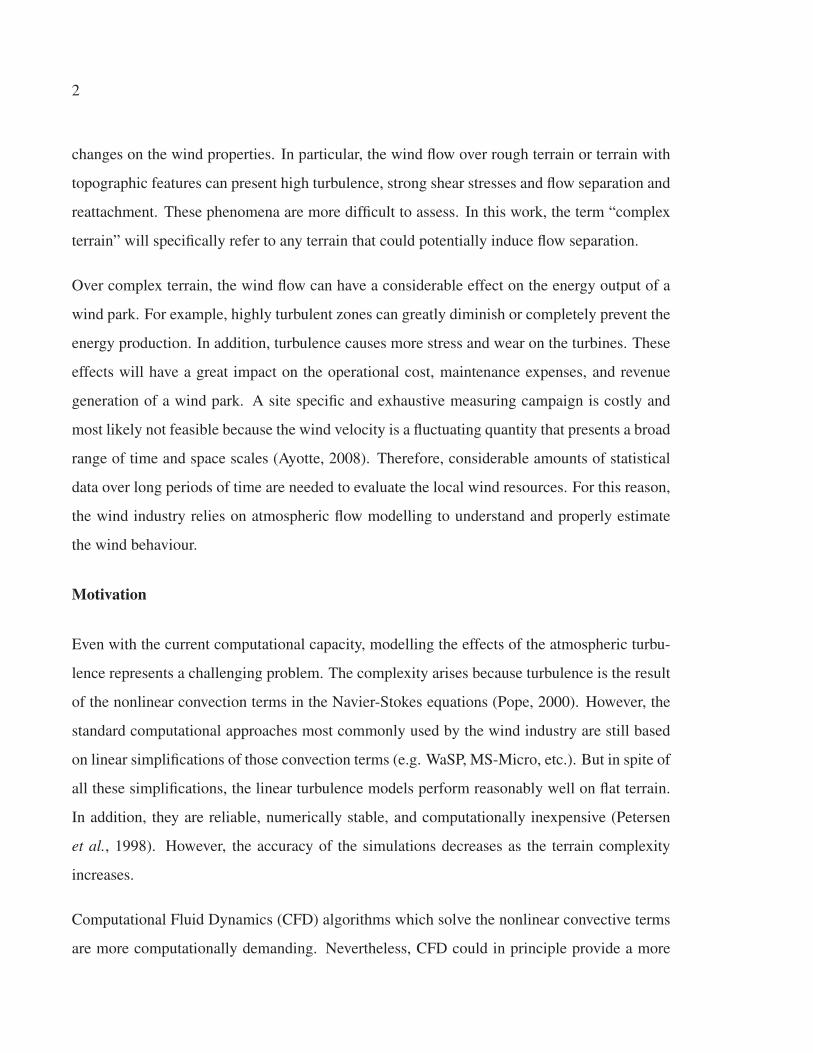
changes on the wind properties. In particular, the wind flow over rough terrain or terrain with

topographic features can present high turbulence, strong shear stresses and flow separation and

reattachment. These phenomena are more difficult to assess. In this work, the term “complex

terrain” will specifically refer to any terrain that could potentially induce flow separation.

Over complex terrain, the wind flow can have a considerable effect on the energy output of a

wind park. For example, highly turbulent zones can greatly diminish or completely prevent the

energy production. In addition, turbulence causes more stress and wear on the turbines. These

effects will have a great impact on the operational cost, maintenance expenses, and revenue

generation of a wind park. A site specific and exhaustive measuring campaign is costly and

most likely not feasible because the wind velocity is a fluctuating quantity that presents a broad

range of time and space scales (Ayotte, 2008). Therefore, considerable amounts of statistical

data over long periods of time are needed to evaluate the local wind resources. For this reason,

the wind industry relies on atmospheric flow modelling to understand and properly estimate

the wind behaviour.

Motivation

Even with the current computational capacity, modelling the effects of the atmospheric turbu-

lence represents a challenging problem. The complexity arises because turbulence is the result

of the nonlinear convection terms in the Navier-Stokes equations (Pope, 2000). However, the

standard computational approaches most commonly used by the wind industry are still based

on linear simplifications of those convection terms (e.g. WaSP, MS-Micro, etc.). But in spite of

all these simplifications, the linear turbulence models perform reasonably well on flat terrain.

In addition, they are reliable, numerically stable, and computationally inexpensive (Petersen

et al., 1998). However, the accuracy of the simulations decreases as the terrain complexity

increases.

Computational Fluid Dynamics (CFD) algorithms which solve the nonlinear convective terms

are more computationally demanding. Nevertheless, CFD could in principle provide a more

3

complete description of the turbulent behaviour and consequently yield more accurate results

in complex terrain. CFD is commonly used by the research community, and in recent years,

the industry has also begun to be use it. However in some instances, the CFD calculation

cost can be excessively high for routine and practical industrial applications. Numerous non-

linear turbulence models have been proposed and used for complex terrain problems. In the

wind community, the most widely studied Reynolds-Average Navier-Stokes (RANS) turbu-

lence model has been the k − ε closure scheme, but many other exist (e.g. Apsley and Castro

(1997), Kim and Patel (2000), Castro et al. (2003), Hargreaves and Wright (2007), etc.). In

general, RANS models yield acceptable results and have a relatively low computational cost;

however, they cannot provide a full description of the turbulence quantities. On the contrary,

the large-eddy simulations (LES) models can be more accurate and complete but they are too

computationally demanding for practical wind energy applications (Ayotte, 2008) (e.g. Dear-

dorff (1972), Mason and Thomson (1987), Sullivan (1994), Andren et al. (1994), etc.). How-

ever, LES might provide some insight and interesting facts about the turbulent behaviour of

the local winds. Hybrid models (e.g. Bechmann (2006), Senocak et al. (2007), etc.), like the

detached-eddy simulation (DES) approaches, incorporate RANS and LES characteristics, and

they could potentially become a good prospect for wind energy simulations.

The wind industry needs accurate turbulence models to understand the wind behaviour over

complex terrain. In addition, these models have to be robust (i.e. reliable and numerically

stable) and practical (i.e. low computational cost). The challenge of this research project is

to analyze a nonlinear turbulence model which could become a good alternative for wind en-

ergy studies over any type of terrain. To attain this goal, the OpenFOAM software has been

chosen for this project (The OpenFOAM Foundation, 2013). This is a community developed

CFD package that allows the users to have full access to the source code. Contrary to the com-

mercial software, the OpenFOAM simulations are not limited or constrained by a predefined

option. The possibility to modify the OpenFOAM code helps tackle specific atmospheric flow

problems and improve the understanding of the wind behaviour.

4

Objectives

The main objective of this research is to adapt OpenFOAM for practical wind energy simula-

tions over complex terrain at a microscale level.

In order to achieve the main goal, the research project is divided into four specific objectives:

1. To select an existing turbulence model that could potentially be a good candidate for

neutral atmospheric boundary layer simulations over complex terrain. To implement the

proposed model in OpenFOAM and to adapt it for wind flow modelling (Chapter 2).

2. To evaluate the advantages and limitations of the chosen turbulence model by analyzing

rather simple but well-known canonical flows (Chapter 3).

3. To identify the appropriate boundary conditions required to correctly model the atmo-

spheric boundary layer over an ideal flat terrain using the proposed turbulence model. To

assess the model performance on flat terrain cases (Chapter 4).

4. To validate the turbulence model against complex flow cases including massively sepa-

rated flows and natural “mildly” complex topography cases (Chapter 5).

Thesis overview

The motivation and detailed objectives of this work have been specified in this introduction.

A literature review concerning the atmospheric boundary layer and its turbulent characteris-

tics is given in Chapter 1. Subsequently, the current state of knowledge regarding atmospheric

flow modelling and the adopted methodology for performing those type of simulations is pre-

sented in Chapter 2. More specifically, this chapter includes a review of the basic concepts

of computational fluid dynamics within the context of the OpenFOAM package (Section 2.1),

the atmospheric modelling techniques (Section 2.1.1), and the recognition of certain important

challenges encountered on microscale simulations (Section 2.2). Taking all this into considera-

5

tion, the k − ω SST-SIDDES hybrid model is proposed to addressed some of those challenges.

This turbulence model is described on Section 2.2.1.

In the present work, a rigorous validation of the turbulence model was performed using some

well-known canonical flows. The results presented in Chapter 3 yield valuable information

about the advantages and limitations of the turbulence model. Additionally, the model has

been tested on atmospheric simulations over flat homogeneous terrain. The results are given

in Chapter 4. Finally Chapter 5, presents complex flow simulations (i.e. massively separated

flows and natural “mildly” complex terrain) using the SIDDES model. A summary of this work

and the most important contributions is given in the conclusion section. To recapitulate, the

turbulence models equations are summarized in Appendix I and Appendix II. Additionally, the

main code lines used for the OpenFOAM v.2.2.2 implementation are described in Appendix III.

Original contributions

The original scientific contributions of this research project are in summary the following:

• The implementation of a hybrid turbulence model for atmospheric flows that

– intrinsically avoids the logarithmic layer mismatch, a problem encountered by al-

most all hybrid models;

– can yield more accurate results on adverse pressure gradients, a phenomenon fre-

quently encountered in complex terrain;

– and has a novel wall treatment which is less dependent on flat terrain assumptions

(Section 2.2.1).

• The development of a complete benchmark to test turbulence models for atmospheric

flows applications. This rigorous validation includes studies on canonical flows and on

flat terrain to understand the inherit limitations and characteristics of a turbulence model

(Chapters 3 and 4).

6

• The modelling of the neutral atmospheric boundary layer over complex flow cases (i.e.

massively separated flows and natural "mildly” complex terrain) accomplished using the

appropriate boundary conditions and the proposed turbulence model without relying on

a wall function (Chapter 5).

CHAPTER 1

THE WIND AND THE ATMOSPHERIC TURBULENT FLOW

The success of the wind energy depends greatly on the proper understanding of the wind be-

haviour and its prediction. The global wind motion is the result of the balance between three

main forces: the pressure differences in the atmosphere, the Coriolis force and the centrifugal

force around zones of low and high pressure (Manwell et al., 2002). In addition, the global

wind patterns are locally modified by the terrain surface (i.e. surface roughness, terrain ele-

vation, etc.). Hence, the wind speed and direction at a particular location is the sum of the

prevailing global air flow and the local effects. The wind can be characterized and studied

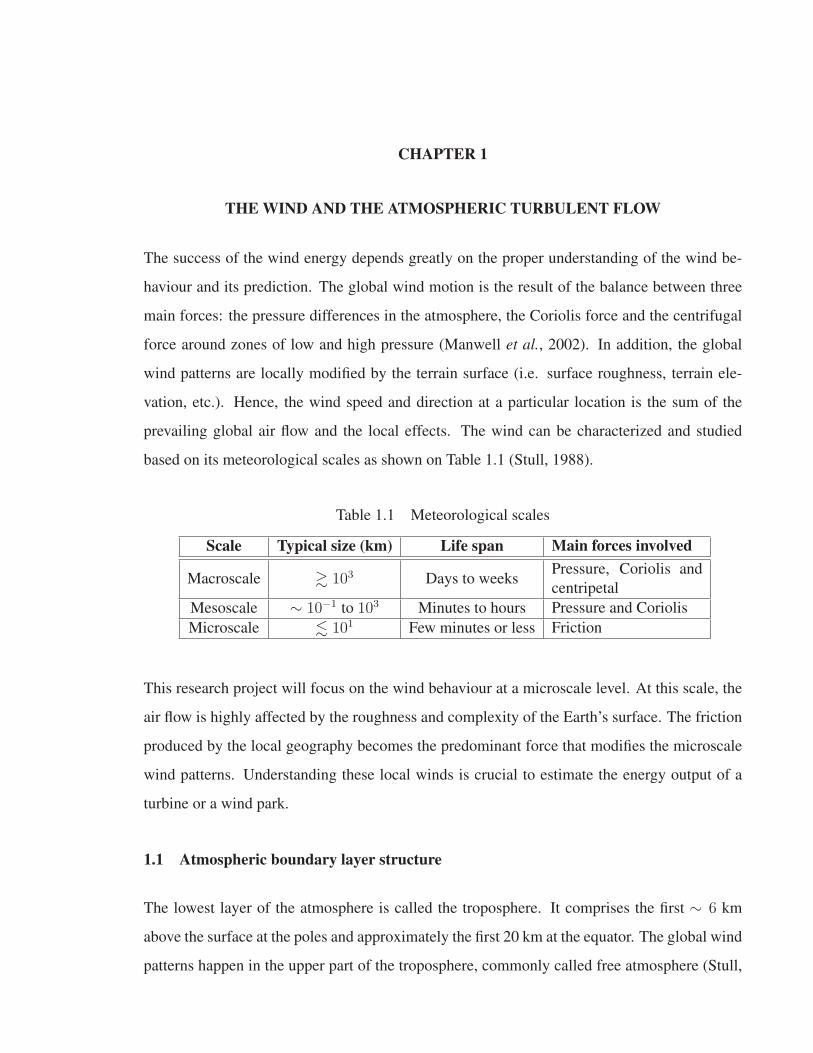
based on its meteorological scales as shown on Table 1.1 (Stull, 1988).

Table 1.1 Meteorological scales

Scale Typical size (km) Life span Main forces involved

Macroscale � 103 Days to weeksPressure, Coriolis and

centripetal

Mesoscale ∼ 10−1 to 103 Minutes to hours Pressure and Coriolis

Microscale � 101 Few minutes or less Friction

This research project will focus on the wind behaviour at a microscale level. At this scale, the

air flow is highly affected by the roughness and complexity of the Earth’s surface. The friction

produced by the local geography becomes the predominant force that modifies the microscale

wind patterns. Understanding these local winds is crucial to estimate the energy output of a

turbine or a wind park.

1.1 Atmospheric boundary layer structure

The lowest layer of the atmosphere is called the troposphere. It comprises the first ∼ 6 km

above the surface at the poles and approximately the first 20 km at the equator. The global wind

patterns happen in the upper part of the troposphere, commonly called free atmosphere (Stull,

8

1988). There, the wind is generally horizontal, non-turbulent and it does not dependent on the

topography. On the contrary, the portion of the troposphere where the wind flow is influenced

by the Earth’s surface is known as the atmospheric boundary layer (ABL). Momentum and

heat transfer processes take place in this layer; hence, the ABL is characterized by high levels

of turbulence (Stull, 1988). It is also where the mesoscale and microscale processes take place.

For wind energy purposes, the ABL is the central focus.

The ABL thickness varies from approximately hundreds of meters to a few kilometres depend-

ing on the terrain and wind speeds, and its variation time scale is of the order of few hours or

less (Stull, 1988). For instance, at daytime the ABL thickness can reach 1-2 km, while at night

with weak winds or coastal regions its thickness is generally around 100 m (Panofsky and Dut-

ton, 1984). Based on the forces involved at different altitudes, the ABL is divided in three

sublayers (Garrat, 1994):

• Roughness or interfacial layer: Just above the Earth’s surface, molecular viscosity

and diffusivity dominate over turbulent transport. Nevertheless, viscous effects are not

significant in atmospheric flow due to their high Reynolds number.

• Surface layer: The Coriolis and the pressure gradient forces are negligible, while the

friction force determines the turbulent air motion. The level of turbulence depends on

the roughness of the terrain and on the obstacles present (i.e. vegetation, hills, buildings,

etc.) The height of the surface layer is approximately 10% of the whole ABL.

• In the upper part of the ABL, the wind flow is influenced by the Earth’s rotation and the

surface friction forces.

Within all these layers, the velocity profiles and turbulence statistics of the wind flow over

flat terrain are relatively simple. Overall, atmospheric turbulence is mainly produced by three

phenomena: the surface shear stress, and the terrain roughness which cause mechanical turbu-

lence, and the vertical heat flux that can produce convective or thermal turbulence. However

if the terrain is not flat, other forces may arise. In uneven terrain, the velocity profiles be-

9

come more complex due to the viscous effects, pressure gradients and acceleration that occur

when the wind flow encounters an obstacle. These phenomena generate additional mechanical

turbulence.

Even though convective turbulence plays a rather important role in the production of atmo-

spheric turbulence (see Panofsky and Dutton (1984) and Stull (1988) for further information

regarding thermal turbulence and atmospheric stratification), this research project will focus on

understanding only the mechanical turbulence caused by the terrain elevation. In other words,

throughout this work it will be assumed that the atmosphere thermal stratification is always

neutral and the surface heating plays a negligible role in the production of turbulence. For this

reason, a temperature equation will not be considered. A neutral stratification happens when

strong winds and overcast skies take place, often late in the afternoon (Stull, 1988). An exact

neutral stratification is not a common occurrence in the atmosphere, however this assumption

greatly simplifies the analysis of the atmospheric flow and allows to isolate and identify the

effects of the mechanical turbulence.

1.1.1 Atmospheric surface layer

Modern wind turbines have a hub height of around 80 to 120 m, while the tip of its rotor blades

can reach up to 120 to 180 m. For the most part, wind turbines reach only the atmospheric sur-

face layer (ASL), thus understanding the effects that take place in this region is crucial. Within

a neutrally stratified ASL over homogeneous flat terrain the vertical variations of the vertical

momentum fluxes are considered negligible. But in fact, the momentum flux (shear τ ) reaches

a maximum at the ground surface and it is null at the top of the ABL. The shear decreases

approximately in a linear manner with height. This means a momentum flux decrease of only

10% within the ASL (i.e. the 10% of the ABL). This 10% variation is often ignored or toler-

ated, thus the momentum flux is considered constant within the ASL (Panofsky and Dutton,

1984).

10

The surface shear stresses τw is commonly used to define a characteristic velocity u∗ called

friction velocity. This parameter is defined as

u2∗ =

τwρ

(1.1)

where ρ is the air density. Based on the assumption that u∗ is constant, the mathematical model

most commonly used to approximate the velocity profiles is the logarithmic law of the wall (or

simply log-law). This log-law defines the streamwise velocity u as

u =u∗κ

ln

(z + z0z0

)(1.2)

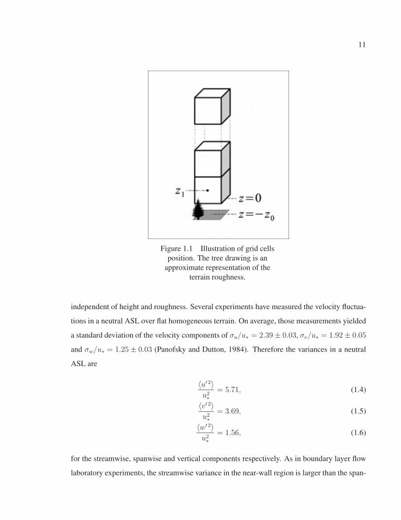
where κ is the von Kármán constant, z the height and z0 the aerodynamic roughness height.

The surface ground is located at a height of −z0 to assure that u(z = 0) = 0. This is illustrated

in Figure 1.1. Notably, the logarithmic law is only valid to describe the surface layer in neutral

conditions over flat and homogeneously rough terrain. Another consequence of the constant

shear stresses, is that the non-dimensional wind shear or mean velocity gradient

〈φm〉 = κz

u∗

∂〈u〉∂z

(1.3)

equals to 1.0 within the ASL. Here 〈·〉 represents an averaged value.

To characterize the conditions of the ASL, the Monin-Obukhov or surface layer similarity

theory defines different scaling parameters (like u∗ and the Monin-Obukhov lengthscale L) and

certain functions (like the logarithmic law and φm). These similarity parameters combine the

effects of the mechanical and the convective turbulence (Panofsky and Dutton, 1984). However

when neutral stratification is being considered, some parameters including the lengthscale L

are not relevant (Stull, 1988). On the contrary, u∗ is important and thus it is often used as a

scaling parameter in surface layer relations.

For purely mechanical atmospheric turbulence, the Monin-Obukhov similarity theory estimates

that the variance of the velocity components (σ2u = 〈u′ 2〉 = 〈(u− 〈u〉) 2〉) is a constant value

11

Figure 1.1 Illustration of grid cells

position. The tree drawing is an

approximate representation of the

terrain roughness.

independent of height and roughness. Several experiments have measured the velocity fluctua-

tions in a neutral ASL over flat homogeneous terrain. On average, those measurements yielded

a standard deviation of the velocity components of σu/u∗ = 2.39± 0.03, σv/u∗ = 1.92± 0.05

and σw/u∗ = 1.25± 0.03 (Panofsky and Dutton, 1984). Therefore the variances in a neutral

ASL are

〈u′ 2〉u2∗

= 5.71, (1.4)

〈v′ 2〉u2∗

= 3.69, (1.5)

〈w′ 2〉u2∗

= 1.56, (1.6)

for the streamwise, spanwise and vertical components respectively. As in boundary layer flow

laboratory experiments, the streamwise variance in the near-wall region is larger than the span-

12

wise and vertical variances (Grant, 1986). Stull (1988) has reported slightly different val-

ues where 〈u′ 2〉/u2∗ = 6.1− 6.5, 〈v′ 2〉/u2

∗ = 2.9− 6.1 and 〈w′ 2〉/u2∗ = 1.0− 2.5. Also Grant

(1991) summarized other aircraft and surface measurements that have yield fairly consistent

results for the ASL variances. Finally as a result of constant variances, the turbulent kinetic

energy

k =1

2

(〈u′ 2〉+ 〈v′ 2〉+ 〈w′ 2〉) (1.7)

has also a constant profile within the ASL.

1.1.2 Above the atmospheric surface layer

The shear stresses are no longer considered constant above the surface layer. For this reason,

the logarithmic law is not longer valid to describe the wind velocity. Vertical velocity pro-

files in the Ekman layer are more elaborated as summarized by Emeis (2013). The variances

parametrization of the turbulent flow above the ASL depends on the height. The normalized

ABL variances relationships are (Stull, 1988)

〈u′ 2〉u2∗

= 6(1− z

H

)2

+z

H

〈u′ 2top〉u2∗

, (1.8)

〈v′ 2〉u2∗

= 3(1− z

H

)2

+z

H

〈v′ 2top〉u2∗

, (1.9)

〈w′ 2〉u2∗

=(1− z

H

)1/2

, (1.10)

where H is the ABL height. The normalized variance at the top of the boundary layer 〈u′ 2top〉/u2

∗

and 〈v′ 2top〉/u2∗ was defined as equal to 2.0 by an experiment carried out by Grant (1986), yet it

can vary (Stull, 1988). In this work, 〈u′ 2i, top〉/u2

∗ = 1.0 as it is defined by Bechmann (2006).

13

1.2 Effects over complex topography

The description of the wind flow over inhomogeneous rough surfaces and over changing topog-

raphy is extremely more complex. In nonuniform terrain, the effects of the wind shear stresses

and turbulence levels depart from well-known equilibrium behaviour of the wind over flat ter-

rain. Thus the homogeneous flat terrain assumptions need to be revised carefully over changing

terrain. For instance, the logarithmic profile is not longer valid in such complex cases because

u∗ is highly dependent on height (Panofsky and Dutton, 1984). It is crucial to understand this

flow behaviour in order to improve the potential of a wind park over nonuniform terrain. A

historical perspective of this problematic is given in Wood (2000).

Reliable measurements of the surface fluxes over complex terrain are unfortunately not always

available or complete. Numerous wind-tunnel experiments also have been carried out, but

due to some conceptual limitations they are not always strictly representative of the ABL (i.e.

the ratio between roughness elements and boundary layer height in the ABL and wind-tunnel

experiments is not always comparable) (Kaimal and Finnigan, 1994). This indicates that our

knowledge about the turbulent processes involved in complex topography is limited. Despite

that, several theories based on linear simplifications have been developed to try to explain the

flow behaviour over nonuniform terrain (including change of roughness and change of surface

elevation). For instance, Jackson and Hunt (1975) derived a two-layer theory to explain the

neutral atmospheric flow over hills. The mean flow around small hills with a downhill slope of

10◦ is well predicted, but the theory fails for steeper hills (Kaimal and Finnigan, 1994). A good

survey of these linear theories can be found on Finnigan (1988) and Athanassiadou and Castro

(2001). It has long been established that a more sophisticated turbulence model is required to

have a quantitative and complete knowledge of the turbulence behaviour. Nonetheless, great

progress has been made in the understanding of how turbulent flow dynamics are affected by

the presence of changing roughness or changing terrain elevation.

When a change in surface roughness takes place over flat terrain, the surface momentum flux

changes, then the air velocity changes and the local equilibrium is lost (Kaimal and Finnigan,

14

1994). To further illustrate this point, if the wind flow is moving from a grass field (z0 = 8 mm)

towards a dense forest region (z0 ∼ 500− 1000 mm) (Panofsky and Dutton, 1984; Manwell

et al., 2002) the surface friction will increase so the flow will slow down. This deceleration

only takes place in the near-wall region, but it is then progressively diffused vertically as the

streamwise distance increases (Kaimal and Finnigan, 1994). Consequently an internal bound-

ary layer is developed. The change in surface roughness will not be studied in this research

project, the focus will concisely placed on terrain elevation changes.

The topography is vaguely classified as flat, hilly and mountainous (Petersen et al., 1998).

The flow around a large hill or a mountains range is predominantly driven by internal grav-

ity waves. The study of gravity wave is beyond the scope of this work, because it is mostly

a mesoscale phenomenon. As for smaller hills which are submerged within the ABL, the

surface stresses, the flow blockage, and the large scale pressure field changes are more impor-

tant. Terrain elevation can considerably increase the momentum exchange in the atmospheric

flow (Athanassiadou and Castro, 2001). Additionally, in purely neutral stratification the verti-

cal movement of an air parcel is only governed by the acceleration cased by terrain constrains;

in reality buoyancy causes a gravitational restoring force that contributes to this vertical move-

ment (Kaimal and Finnigan, 1994).

Neutral atmospheric flow accelerates when it encounters an obstacle because of the pressure

gradients that developed around it. Downstream of the obstacle, wake vortices, separation,

back-flow and reattachment regions could be present. Separation occurs when the flow direc-

tion reverses, namely when the velocity vertical gradient at the wall is

∂u

∂n

∣∣∣∣w

< 0. (1.11)

For laminar flows, the separation point takes place when the surface stress τw = μ(∂u/∂z)|w is

zero. Nevertheless it is not evident when the separation point occurs for turbulent flow due to

the complicated turbulent response (Kaimal and Finnigan, 1994). Scientists rely on empirical

and qualitative data to predict a separation point. For a smooth slope hill, the critical slope angle

15

that will most likely produce separation is around 18◦. Even when the topography effects are

expected to dominate, the critical angle is highly dependent on the ground surface roughness.

The angle for separation diminishes as the the surface roughness increases (Kaimal and Finni-

gan, 1994). Additionally, it has been observed that a separation region in turbulent flow is an

unsteady process (Ayotte, 2008).

Other interesting phenomena take place when comparing the flow around two-dimensional

hills (elongated ridges) against three-dimensional hills. When the wind flow encounters a

two-dimensional hill, the flow decelerates at the foot of the hill, then accelerates and reaches

a maximum at the top of the hill (Kaimal and Finnigan, 1994), finally if separation occurs

one closed bubble is formed (Apsley and Castro, 1997). In contrast when the wind comes

across a three-dimensional hill, the flow does not decelerate at the foot of the hill, instead the

flow is redirected laterally. Also if a separation region develops, two counter-rotating vortices

developed, and the separation bubble has a constant inflow and outflow (Kaimal and Finnigan,

1994).

Lastly, measurements show that the vertical velocity variance 〈w′ 2〉 at the ASL does not seem

to be affected by the presence of uneven terrain. This is because the vertical velocity fluctua-

tions are produced by small eddies that can rapidly adjust to the topography changes. On the

contrary, the streamwise fluctuations are governed by large eddies that can only adjust slowly

to the changing terrain. Compared to flat terrain, the streamwise variance 〈u′ 2〉 tends to be

smaller (larger) when the locally surface stresses are larger (smaller) than the upstream condi-

tions (Panofsky and Dutton, 1984). For instance on hilltops or in a smooth-to-rough transition,

the local shear stresses are larger thus the streamwise variance will most likely be smaller than

the flat terrain variances. For this same reasons, the vertical velocity spectra over flat and com-

plex terrain are similar. As for the horizontal velocity spectra (refer to Section 1.3), they differ

at the small wavelength (big eddies) between flat and complex terrain observations, but are

similar in the high wavelength (small eddies) region (Panofsky and Dutton, 1984).

16

1.2.1 Turbine micro-siting

The placement of a turbine is a challenging problem but crucial for the proper operation of a

wind park. The criteria used to define the ideal siting arrangement of the turbines is mainly

based on the maximization of the total energy production. The power P produced by a wind

turbine can be estimated by

P =1

2ηmechCPρAu

3 (1.12)

where u is the air velocity, ρ is the air density, A is the area swept by the turbine rotor, ηmech is

the rotor mechanical and electrical efficiency, and CP is the machine power coefficient (Man-

well et al., 2002). This evaluation of the turbine power, it based on the assumption that the

air flow is always perpendicular to the rotor with a constant and uniform velocity, and that

the turbulence intensity is low. The turbulence intensity is defined as TI = urms/〈u〉, where

urms is the root-mean-square of the velocity and 〈u〉 is the mean velocity. However in reality,

a higher turbulence intensity may result in an increased energy output for smaller wind speed

values, but in a reduction of the turbine power for faster winds (Langreder et al., 2004). A more

exhaustive analysis demonstrated that the parameters that affect the most the performance and

power production of a turbine are: the wind speed at hub height, then the turbulence intensity

and lastly the wind shear (Clifton et al., 2014).

Furthermore higher turbulence levels, as well as the separation and reattachment of the air flow,

can generate important vibrations on the turbine blades and several problems can arise. Specif-

ically, those variable winds increase the mechanical stresses on a turbine, incrementing the

fatigue loads, wear and possibilities of damages (Peinke et al., 2004) (for a detailed study of

the effects of turbulence intensity in the fatigue loads of turbines, refer to Riziotis and Voustsi-

nas (2000)). These effects will have a great impact on the operational cost, maintenance ex-

penses, and revenue generation of a wind park. For instance for the same wind speed, the

damaged caused by the equivalent loads on the blade roots can increase up to three-times if

the turbulence intensity varies from 10% to 25% (Clifton et al., 2014). Another example is

17

a study carried out in an Austrian wind park located in a mountainous terrain. In this area,

the turbulence intensity was more than 20% and the energy generation yield 25% less than the

estimated calculation (Clifton et al., 2014). Consequently, for wind turbine siting is essential

to understand the magnitude of the wind acceleration and turbulence as well as the position

where these phenomena take place (Kaimal and Finnigan, 1994).

1.3 Turbulence

Irregular motion, continuous instability, nonlinear behaviour and randomness are some of the

essential features of turbulent flows. More precisely, the main turbulence characteristics are

the efficient transport and high mixing rate of momentum, kinetic energy and matter through

a fluid (Tennekes and Lumley, 1972). Additionally, turbulence is always a dissipative phe-

nomenon (Wilcox, 2004).

A turbulent fluid presents a broad and continuous range of time and length scales (Wilcox,

2004). An approach to visualize these scales is to treat the local swirling motion of the

fluid as turbulent structures, or eddies, with characteristic length and time scales. Overall,

the large scales do most of the transport of momentum and the production of turbulent ki-

netic energy, which is then transferred to the smaller scales mainly by inviscid processes (i.e.

vortex stretching, etc.) and finally the smallest scales dissipate that energy by viscous pro-

cesses (Tennekes and Lumley, 1972). This concept is known as the turbulent energy cascade.

The anisotropy of the turbulent eddies is another relevant parameter. Large eddies are gener-

ally anisotropic and highly dependent on the flow boundaries, while the small scale eddies are

isotropic according to Kolmogorov’s theory (Kolmogorov, 1941).

A Fourier analysis of a turbulent velocity field can be used to mathematically represent certain

properties of the turbulent flow and visualize the energy cascade. For instance, the velocity

spectrum E(κ) represents the energy distribution over different lengthscales l characterized

by the wavenumber κ = 2π/l. The spectrum of real physical turbulence at sufficiently high

Reynolds number should display at least three distinct sections. The portion of the spectra at

18

small κ (or large l) represents the energy-containing eddies where the energy is produced, the

middle section called the inertial subrange depicts the transfer of energy which is governed by

inertial processes, and the dissipation range at the larger and isotropic κ where viscous effects

are predominant. Additionally, the well-known Kolmogorov theory predicts that the inertial

subrange on this spectrum has a slope of −5/3 (Kolmogorov, 1941).

According also to the Kolmogorov theory, the small eddies dissipation rate depends on the

kinematic viscosity ν and on the rate at which the large eddies supply energy ε. Based on

this principle, the characteristic scales of the smaller eddies can be defined. These parameters,

called the Kolmogorov scales, are the length η, the time τ and the velocity υ. Hence,

η =(

ν3

ε

)1/4

, τ =(

νε

)1/2

, υ = (νε)1/4. (1.13)

These parameters imply that the small turbulent scales are statistically similar and universal for

high Reynolds flows (Kolmogorov, 1941).

Characterizing a random turbulent field can be mathematically complex. In experiments or

simulations of turbulent flows, several types of averaging are defined in an attempt to get a

global and more simplified picture of the turbulence. For example, statistically stationary flows

can be described by the time average of its velocity field

〈u (t)〉t = 1

T

∫ t0+T

t0

u (t′)dt′, (1.14)

whereas a spatial average can be defined for homogeneous turbulence

〈u (t)〉s = 1

V

∫ V

0

u (x, t)dV (1.15)

19

in one, two or three dimensions. And finally, if a flow experiment can be replicated N times,

an ensemble average

〈u (t)〉N =1

N

N∑n=1

u(n) (t) (1.16)

can be used (Pope, 2000). For practical reasons, it is not always possible to repeat an experi-

ment or a simulation, so 〈u〉N is rarely computed for atmospheric flows. Under certain circum-

stances, the ergodicity principle states that ensemble averages are equivalent to time averages.

Similarly, 〈u〉t ≈ 〈u〉s for some cases based on the Taylor hypothesis1 (Panofsky and Dutton,

1984). In this work, 〈u〉t and 〈u〉s, 〈u〉N will be expressed as 〈u〉 to simplify the notation.

However, the procedure used to compute the average values will always be clearly stated.

1.4 Microscale flow governing equations

In order to study the atmospheric flow at a microscale level, a mathematical description of the

turbulent flow is needed. Using the Einstein notation2, the unsteady behaviour of an incom-

pressible fluid is described by the Navier-Stokes or momentum equations

∂ui

∂t+

∂ujui

∂xj

= −1

ρ

∂σij

∂xj

+Fi

ρ, (1.17)

and the mass continuity equation

∂ui

∂xi

= 0. (1.18)

Here ρ represents the constant density, ui the velocity, t the time, and xi the Cartesian coordi-

nates. Additionally, ∂σij/∂xj characterizes the surface forces, while Fi the body forces acting

on a fluid (Panton, 1995).

1The Taylor hypothesis is not quite valid for atmospheric flows since its basic assumptions are not entirely

satisfied. First, the turbulence evolves over time so it is not frozen as assumed by the theory; secondly, the eddy

convection velocity is not always precisely the local mean speed. Due to the lack of a better option, the Taylor

hypothesis is widely used in atmospheric flows (Kaimal and Finnigan, 1994).2 u = uiei = (u, v, w)

20

The different surface forces are summed up in the total stress tensor σij . It comprises the effects

of the pressure p (a normal stress) and the shear stresses τij , hence

∂σij

∂xj

= − ∂p

∂xj

δij +∂τij∂xj

(1.19)

where δij is the Kronecker delta. Additionally, the shear stress or viscous stress are given by

τij = μ(∂ui

∂xj

+∂uj

∂xi

)(1.20)

where μ is the dynamic viscosity of the fluid. As for the body forces, Fi can represent the

Coriolis force, the centrifugal force, a large scale pressure gradient, etc.

By substituting Equations 1.19-1.20 into Equation 1.17, the derivative form of the Navier-

Stokes equations can be rewritten as

∂ui

∂t+

∂ujui

∂xj

= −1

ρ

∂p

∂xi

+∂

∂xj

[ν

(∂ui

∂xj

+∂uj

∂xi

)]+

Fi

ρ, (1.21)

where ν = μ/ρ is the air kinematic viscosity. It is not easy to solve the turbulent momentum

equations because of the nonlinear term ∂(ujui)/∂xj , and the fact that the pressure and the

velocity fields are coupled (Ferziger and Peric, 2002). In most cases, these equations cannot be

solved analytically, therefore numerical methods are needed to model and to approximate the

turbulent flow behaviour.

CHAPTER 2

MICROSCALE ATMOSPHERIC FLOW MODELLING

The partial differential equations that describe the atmospheric turbulent flow are rather com-

plex and can only be solved numerically. Computational Fluid Dynamics (CFD) is a interdisci-

plinary branch of science which relies on numerical methods and algorithms to solve these type

of equations through computer simulations. Special software, like OpenFOAM (Open Source

Field Operation and Manipulation), have been designed to tackle CFD simulations and analyze

fluid problems. In this section, only a brief summary of the basic aspects of CFD will be given.

For a more complete reference see Ferziger and Peric (2002). This section will describe the ba-

sic concepts of CFD within the context of OpenFOAM and atmospheric flows at a microscale

level. This chapter is also an attempt to gather the relevant information on the subject in one

place and contribute to the OpenFOAM documentation for microscale atmospheric flows.

2.1 Basics aspects of computational fluid dynamics

A CFD analysis involves two fundamental aspects: the physical modelling (i.e. turbulence

models) and the numerical techniques (i.e. effective, robust and reliable methods to discretize

and solve the linear system of equations). More specifically, the CFD process starts by the

derivation the partial differential (or integral) equations that govern a flow field (as done in

Section 1.4). The resulting equations for the turbulent atmospheric flow are nonlinear, mathe-

matically complex and computationally demanding to solve. A turbulence model is needed to

approximate and simplify the physics, and to alleviate the computational cost. Additionally, a

CFD computation depends on the discrete treatment of a continuous fluid. Consequently the

space domain that represents the fluid volume is divided into cells or control volumes (CV)

that form a grid or mesh. If required, the time domain is also divided in time steps. The partial

differential equations are also discretized to obtain a set of approximate algebraic equations for

each cell or control volume. Finally the discretized equations are then solved using numerical

methods to find an approximate solution (Ferziger and Peric, 2002).

22

2.1.1 Physical modelling

As previously mentioned, turbulence models are required to approximate or estimate the non-

linear convective term present in the Navier-Stokes equations. Several classes of turbulence

models have been developed. Here, only a brief description Reynolds-averaged Navier-Stokes

(RANS) models, large-eddy simulation (LES) models and a hybrid technique called detached-

eddy simulations (DES) will be given. A more complete description of turbulence models can

be found in Pope (2000) and Wilcox (2004).

A turbulence model estimates the nonlinear term by making different assumptions about the

turbulence characteristics and by computing additional turbulence quantities or transport equa-

tions. In general, the main difference between those turbulence models is the level of descrip-

tion of the turbulent flow, in other words, which turbulent scales are explicitly resolved by the

equations and which ones are simply estimated or modelled.

Reynolds-averaged Navier-Stokes (RANS)

RANS models are based on the Reynolds decomposition of the turbulent velocity field. Con-

sequently the instantaneous velocity ui is expressed as the sum of the time-averaged velocity

〈ui〉, and the instantaneous fluctuation u′i, thus (Reynolds, 1895)

ui(x, t) = 〈ui〉(x, t) + u′i(x, t) (2.1)

Then the time-averaged flow Navier-Stokes equations used by any RANS model can be ob-

tained by substituting Eq. 2.1 into the Navier-Stokes momentum expression (Eq. 1.21). This

yields

∂〈ui〉∂t

+∂〈uj〉〈ui〉

∂xj

= −1

ρ

∂〈p〉∂xi

+∂

∂xj

[ν

(∂〈ui〉∂xj

+∂〈uj〉∂xi

)− 〈u′

iu′j〉]+

Fi

ρ. (2.2)

23

The term 〈u′iu

′j〉 is called the turbulent stress tensor or the Reynolds stress tensor. The presence

of these stresses in the equation show that the velocity fluctuations do have an impact on the

mean velocity.

The time averaging procedures has introduced nine more variables (one for each Reynolds

stress component) which are unknown (White, 1991). This system of four equations has more

than four unknowns (〈ui〉, 〈p〉 and 〈u′iu

′j〉), thus it is not mathematically closed. Therefore,

a closure scheme is required to determine the nonlinear Reynolds stresses. One of the most

common approaches is to use the turbulent viscosity or Boussinesq hypothesis which states

that

−ρ〈u′iu

′j〉 = νt

(∂〈ui〉∂xj

+∂〈uj〉∂xi

)− 2

3kδij (2.3)

where k = 0.5〈u′iu

′i〉 is the modelled turbulent kinetic energy and δij is the Kroneker

delta (Boussinesq, 1897). Also the turbulent or eddy viscosity νt is a newly introduced variable

can only be modelled or empirically approximated by introducing extra transport equations.

For example, the k − ω SST RANS model uses the specific turbulent kinetic energy and the

specific dissipation rate equations (k and ω respectively) to model νt. Finally, the time-averaged

momentum equation is given by

∂〈ui〉∂t

+∂〈uj〉〈ui〉

∂xj

= −1

ρ

∂〈p〉∂xi

+∂

∂xj

[(ν + νt)

(∂〈ui〉∂xj

+∂〈uj〉∂xi

)]+

Fi

ρ. (2.4)

RANS models solve only the time-averaged velocity field and model the velocity fluctuations.

For this reason they do not provide any information about the instantaneous behaviour of the

flow nor about the turbulent structures, but the required computational power is relatively low.

For steady RANS models the time derivative is zero. But if ∂〈ui〉/∂t �= 0, transient phenomena

of a much bigger time scale than the turbulent fluctuations can be simulated. In other words,

the low frequency variations in the diurnal cycle of the atmosphere can be estimated (Koblitz

et al., 2013), but not the turbulent fluctuations nor the intermittent separation bubble behind a

hill. These transient models are called unsteady-RANS (URANS).

24

RANS and URANS simulations generate fairly accurate results for winds over flat terrain.

However, the results obtained over complex terrain are not always reliable or numerically sta-

ble (Bechmann and Sørensen, 2010). In general, the flow patterns in adverse pressure regions

are not well predicted. For instance, RANS models are not always able to reproduce the flow

separation on the lee-side of a hill because they usually predict low velocity and low turbulence

intensity (Bechmann and Sørensen, 2010). A RANS model called k − ω SST is commonly

used for aerodynamic flows. It yields fairly accurate results on adverse pressure gradients and

separation regions, and its results are more accurate on the viscous near-wall regions than for

example the RANS k − ε turbulence model (Menter, 1992). However, the k − ω SST model

has rarely been used for atmospheric flows. In this thesis, the advantages of the model will be

investigated in ABL simulations.

Large-eddy simulation (LES)

In LES a spatial filtering operation is carried out to decompose the velocity field as

u(x, t) = u(x, t) + usgs(x, t). (2.5)

u is the filtered or resolved component which represents the larger three-dimensional unsteady

turbulent scales that will be explicitly solved; while usgs is the residual or subgrid component

which will be modelled. The filtering is defined as

ui(x, t) =

∫ui(x− r, t)G(r,x)dr (2.6)

where G is a normalized filter function (Leonard, 1974). Several types of filters exist (e.g.

box, Gaussian, sharp spectral, Cauchy, and Pao), but most often the grid spacing Δ acts as the

filter width (See Pope (2000) for details). Eddies which are twice as large as the cell size are

explicitly solved. This is deduced from the Nyquist theorem (Kaimal and Finnigan, 1994). The

filtered velocity equations can be found by filtering the Navier-Stokes equations. Analogous to

the Reynolds decomposition, the filtering operation yields a residual (or sgs) stress tensor that

25

can only be modelled by a closure scheme. The LES momentum equation using a turbulent or

eddy viscosity model are then given by

∂ui

∂t+

∂ujui

∂xj

= −1

ρ

∂p

∂xi

+∂

∂xj

[(ν + νt)

(∂ui

∂xj

+∂uj

∂xi

)]+

Fi

ρ. (2.7)

This time the turbulent viscosity νt, represents the effects of the residual or sgs motions.

Solving the LES equations yields information about the unsteady filtered field. Then, the

filtered velocity can be decomposed into a (time or spatial) average value 〈u〉 and filtered

fluctuations u′; hence (Bechmann, 2006)

u = 〈u〉+ u′. (2.8)

Consequently, the instantaneous velocity field is

u = u+ usgs,

u = 〈u〉+ u′ + usgs. (2.9)

Contrary to RANS, the LES models can give a more complete description of a turbulent flow.

LES can provide information about the unsteady nature of the turbulence by resolving certain

fluctuations in the flow. For example, LES can predict unsteady effects in wind flow over hills

like the instantaneous and intermittent separation on the lee-side (Ayotte, 2008). This important

phenomenon cannot be simulated using RANS models.

The grid used on LES cases should have near-cubic cells to avoid imposing non-physical ef-

fects to the large isotropic turbulence structures; however, close to the wall the flow is highly

anisotropic, and the grid is usually refined (Wood, 2000). For the atmospheric flow in general,

an appropriate LES grid can be relatively coarse far away from the Earth’s surface (Bech-

mann and Sørensen, 2010). However, for resolving the near-wall eddies instead of just mod-

elling them, a finer grid is needed. Since the grid resolution required to resolve these small-

scale eddies increases approximately as the square of the Reynolds number, LES can be com-

26

putationally demanding (Gungor and Menon, 2010). The expensive computational cost makes,

to this day, LES not suitable for industrial wind energy computations; however, LES can have

important scientific implications thanks to the detailed flow behaviour that can be predicted.

Detached-eddy simulation (DES)

The standard detached-eddy simulation (DES) is a hybrid technique which uses a URANS

model to solve the flow behaviour in the boundary layer and a LES model in regions of detached

flow (Spalart et al., 1997), as the sketch in Figure 2.1a shows. The DES technique can poten-

tially improve the prediction of the flow behaviour with respect to a RANS models (Menter

et al., 2003), however, it has two well-known inherent deficiencies. First, the standard DES

can sometimes predict unphysical separation regions in certain types of grids (Menter et al.,

2003). This phenomena is called grid-induced separation (GIS). Secondly, if the grid spacing

(streamwise and spanwise) is much smaller than the boundary layer height, the DES model

can act as a wall-modelled LES (WMLES) (Spalart et al., 2006). In this case, the URANS

branch of the hybrid model will solve the flow only in the near-wall region and not in the entire

boundary layer, whereas the LES branch will compute the flow away from the wall but still

inside the boundary layer. Figure 2.1b depicts the WMLES behaviour of the hybrid model.

This not in agreement with the original formulation of the DES model1. It has been shown that

a WMLES based on the DES equations is robust and able to sustain turbulence, however, it

may lead to inaccurate velocity and stress values at the URANS and LES interface causing a

log-layer mismatch (LLM) (Nikitin et al., 2000).

A modification to the standard equations of DES was proposed to eliminate the hybrid model

dependency on the grid density. This is achieved by using a shielding function that main-

tains the RANS behaviour within the boundary layer (Spalart et al., 2006). This newer ap-

proach, known as the delayed detached-eddy simulations (DDES) model, solves the GIS prob-

lem but it does not address the disadvantages of the LLM. Fortunately, the improved delayed

1Rigorously, a WMLES based on the DES equations should not be called “DES” (Spalart et al., 2006). Nev-

ertheless for simplicity in this thesis, DES will refer to the model that uses the standard DES switch Equation 2.20

regardless of the type of mesh.

27

(a) Standard use of DES(b) WMLES usage

Figure 2.1 Sketch of DES applications. The extent of the boundary layer is

represented by the colour blue. (a) The original DES was conceived to use URANS in

the boundary layer, and LES everywhere else. (b) As a WMLES, the hybrid model

employs URANS in the near-wall region, and LES far from the wall but within the

boundary layer.

detached-eddy simulations (IDDES) model includes additional modifications that deal with the

LLM (Shur et al., 2008). The main disadvantage of IDDES is that the formulation increases

considerably the complexity of the model. A simplified version of IDDES (hereafter SIDDES)

has been recently proposed and successfully tested on aerodynamic flows (Gritskevich et al.,

2012). The SIDDES results are consistent with IDDES, hence the use of the simplified model

is justified.

The wind energy microscale simulations are focused essentially only on the boundary layer;

thus the hybrid model aim is to use URANS only in the near-wall region and LES away from

the wall but still inside the boundary layer. In other words, the type of meshes needed (i.e.

finer in the streamwise and spanwise direction compared to the height of the boundary layer)

will force a standard DES model to always behave as a WMLES. Consequently, the use of

the standard DES technique is not entirely adequate and it is extremely important to correct

the LLM problem on ABL simulations. On the contrary, the GIS is not a relevant issue for

atmospheric simulations. The performance and viability of the SIDDES turbulence model for

neutral ABL cases will be analyzed. A full description of the proposed model will be given on

Section 2.2.1.

28

Surface boundary conditions in atmospheric flows

Boundary conditions are required to solve a CFD simulation. They vary depending on the prob-

lem to be solved, but certain guidelines should be followed (Franke et al., 2007). The boundary

conditions for each simulated case will be specified in the following chapters. However, the

solid surface boundary condition requires especial considerations.

The standard no-slip condition (uwall = 0) can be defined on smooth surfaces for the velocity

at the nearest wall node z1 provided that the turbulence model equations can be accurately

solved down to wall (Batchelor, 1967). However for high Reynolds flows, an extremely large

number of cells are needed to solve the near-wall flow; for this reason, wall functions are

usually imposed. For instance, a wall function imposes a value of the velocity at z1 assuming a

log-layer profile; thus, a wall function is valid only if the first grid node near the wall is located

within the logarithmic region (30 < z+1 = u∗z1/ν) (White, 1991). As for rough surfaces in

turbulent flows, the roughness has a great impact on the viscous sublayer and it rather increases

the wall friction (White, 1991). If the terrain is considered to be rough, a wall function is

commonly imposed to model the drag caused by this roughness.

It has been shown that adding a wall function generates accurate results on attached aerody-

namic flows (Piomelli et al., 1989), whereas their accuracy on separated flows has not been

confidently established (Stoll and Porté-Agel, 2006). Notably in theory, a wall function is not

longer valid and it might not yield accurate results in complex geometries or terrain were strong

adverse pressure gradients, and separation, reattachment or recirculation regions exist (Patel,

1998; Ferziger and Peric, 2002).

The wall functions for RANS and LES vary slightly due to the computed variables (i.e. fluctu-

ating vs. mean velocity), yet the basic principle is the same (Ferziger and Peric, 2002). Several

approaches have been implement to model the atmospheric flows surface boundary conditions,

Stoll and Porté-Agel (2006) provide a good summary of the most relevant wall functions used

for LES. In essence, all of those wall functions relate the surface shear stresses to the velocity

at the nearest node to the wall assuming a logarithmic-law velocity profile. Those wall func-

29

tions rely on the Monin-Obukhov similarity theory (i.e. log-law on rough flat terrain only and

based on ensemble averages) to calculate the surface shear stresses, and it is not clear how

these wall functions behave specially on complex terrain. Some studies have shown that for

example the level of velocity fluctuations is underestimated for most of the wall functions used

on flat terrain cases (Stoll and Porté-Agel, 2006). Those errors can be propagated throughout

the surface layer. Due to the lack of a better solution, the use of standard wall functions is

a common practice for ABL simulations over complex flows. The ability to compute a more

reliable surface boundary condition for high Reynolds flows over rough and complex terrain is

one of the biggest challenges that the CFD community currently faces (Piomelli et al., 1989;

Chow, 2004; Stoll and Porté-Agel, 2006).

A different approach to the standard wall function is explored within this work by using the

k − ω SST turbulence model. This model chosen mainly for two reasons. First, the model

can be integrated down to the wall (Menter, 1994) if a proper mesh is used; and secondly, the

original turbulence model equations directly account for surface roughness (Patel and Yoon,

1996). These characteristics are particularly advantageous because the used of standard wall

functions can be avoided.

2.1.2 Numerical techniques in OpenFOAM

The OpenFOAM software framework is used to perform all the atmospheric flow simulations

of this work. A brief description of the numerical aspects of CFD concerning the atmospheric

flow in the OpenFOAM context will be given. OpenFOAM uses one of the most common

discretization approaches called Finite Volume Method (FVM) which solves the integral form

of the momentum equations in each CV on the grid. This method relies on the fact that fluxes

must be conserved in each control volume and hence conserved globally (Ferziger and Peric,

2002). Then by using the Gauss’ divergence theorem, some of the volume integrals of these

equations (i.e. the convective and diffusive term) are converted into surface integrals over the

CV to estimate the fluxes (Versteeg and Malalasekera, 2007). Whereas the other terms in the

equation (i.e. source terms) can easily be treated as volume integrals.

30

To compute exactly a surface integral, the value of the integrand quantity f needs to be known

everywhere over such surface. Since this is not possible, an approximation is required. Open-

FOAM assumes that the value of any quantity is constant over a surface (Churchfield et al.,

2010) and equivalent to the mean value over such surface. This is called the midpoint rule ap-

proximation and it provides a second-order accuracy (Ferziger and Peric, 2002). More specifi-

cally, the value of the surface integral at a CV face located at point ‘e’ is estimated as

Fe =

∫Se

f dS = 〈f〉Se ≈ fe Se, (2.10)

thus the product of the integrand at the cell-face centre fe times the cell-face surface area Se.

As for the volume integrals a similar approximation can be made, but in this case, the value

of a variable q is computed at point ‘p’- the CV centre. Therefore, the value of the volume

integral is

Qp =

∫V

q dV = 〈q〉ΔV ≈ qp ΔV. (2.11)

Here qp is the known value of a quantity at the cell centre, so no interpolation is needed.

Such volume integral is exact if q is constant or varies linearly within the CV, otherwise it

becomes a second-order approximation (Versteeg and Malalasekera, 2007). For these reasons

OpenFOAM has intrinsically a second-order spatial discretization.

Those surface and volume integrals need certain values of variables and/or gradients that

are not always located at a central node, therefore, further interpolation from cell centres to

cell faces values are required. Numerous interpolation schemes have been developed, for

example: upwind interpolation (UDS), linear interpolation2 (CDS), quadratic upwind inter-

polation (QUICK), etc.), which have different levels of accuracy (e.g. first-order, when the

truncation error is the order of (Δx), second-order with a truncation error in the order of

(Δx)2, etc.). For specific details of each discretization scheme refer to Anderson (1995), Ver-

steeg and Malalasekera (2007) and Ferziger and Peric (2002). Several interpolation schemes

2Linear interpolation corresponds to central difference approximation for finite difference methods, therefore

the CDS label.

31

are already coded in OpenFOAM thus this research work will not focus on modifying or im-

plementing new schemes. However, it will be verified that the schemes are stable and that the

numerical dissipation is minimal leading to physical results. The interpolation methods and its

particular parameters are specified in OpenFOAM simulation in the fvSchemes input file; an

example of such file used for atmospheric flow simulations is shown on Appendix III.6.

The velocity and pressure discretized field are computed using the pressure-implicit split-

operator (PISO) algorithm (Issa, 1985). PISO is a non-iterative method that solves the

momentum-pressure coupling of the discretized flow equations implicitly in time. Several

sets algebraic equations or matrices have to be solved within the different steps of the PISO

algorithm. To find a solution for those matrices, numerous methods or techniques are al-

ready implemented in OpenFOAM. They will not be discussed here because the subject is

extensive and numerous good reference exist including Ferziger and Peric (2002) and Ver-

steeg and Malalasekera (2007). The solution techniques and its particular parameters are spec-

ified for an OpenFOAM simulation in the fvSolution input file; an example of such file used

for atmospheric flow simulations is shown on Appendix III.7.

The PISO algorithm consist generally in one predictor step and two correctors steps which

provides a velocity and pressure solution that are respectively third and second-order accurate.

Adding another corrector loop will increase the accuracy by one order (Issa, 1985). Since

OpenFOAM has a second-order spatial discretization, extra corrector loops might be unnec-

essary. However, it was observed that setting three corrector steps (nCorrectors variable in

the fvSolution file) the solution converged faster and the number of total pressure iterations

was greatly reduced. Additionally, the OpenFOAM structure is based on a collocated grid,

thus all the variables are stored at the centre of the CV. This can generate unphysical pressure

oscillations in the solution (Patankar, 1980). To avoid those oscillations, OpenFOAM uses

a method similar to the Rhie-Chow correction within the PISO loop to obtain a oscillation-

free field (Peng-Karrholm, 2006). This is one of the reasons why the PISO method in Open-

FOAM (Peng-Karrholm, 2006; Churchfield et al., 2010) varies slightly from the original PISO

formulation (Issa, 1985) which was developed for staggered grids.

32

Systematic errors are always present in any numerical simulation. The accuracy of the solu-

tion depends on modelling, discretization and iteration errors (Ferziger and Peric, 2002). To

correctly assess the modelling errors a comparison with experimental data has to be done. Un-

fortunately, precise measurements are essential and not always available. However the known

inaccuracies or assumptions of the turbulence model that could lead to some modelling errors

will be stated and a full validation of the turbulence model will be carried out. Concerning

the discretization errors, all the discretization schemes used will be second-ordered accurate in

time and space. Additionally, a grid independence and convergence should be verified; how-

ever, in wind engineering problems, this is not always attainable. Doing a grid-independence

test with even finer grids is not always possible because the cost of coarse grid is already too

high. In addition, a finer grid in LES will resolve smaller eddies and might yield a different

solution. For these reasons, it is hard to judge the effect that these discretization errors have on

the results (Bechmann, 2006). Finally to limit the iteration error, a convergence tolerance of at

least 10−6 will be set in the fvSolution file for the normalized equation residual.

2.1.3 Additional details of the OpenFOAM framework

OpenFOAM software an open-source code developed in C++; in other words, the user can

modify the code if necessary and adapt it to his or her needs. This is an important advantage of

OpenFOAM, since the commercial software are not always as flexible.

In general, OpenFOAM works by creation of executable files called applications. The solver

applications are used to solve a particular problem, while the data handling (pre-processing and

post-processing) is done by the utility applications (The OpenFOAM Foundation, 2013). The

user can select the grid discretization, the boundary conditions, the discretization schemes, the

level of accuracy, and other parameters.

The software contains many features already defined and implemented (e.g. several turbulence

models (RANS and LES), wall functions, boundary conditions, data sampling, etc.). Nonethe-

less, not all the requirements needed for the completion of this research project are satisfied.

33

Several aspects of the OpenFOAM code had to be modified for this project. These code changes

are related to the improvement of ABL modelling, and the adaptation of the turbulence model

and boundary conditions. The main code adaptations are described on Appendix III.

2.2 Challenges in microscale wind energy simulations

Now that the basis of CFD and the OpenFOAM framework have been discussed, a more in-

formed and critical approach to solve some of the wind energy challenges can be taken. Two of

the main challenges that the wind industry faces when doing microscale CFD simulations is the

high computational cost, and the fact that most surface treatments are based theories developed

for equilibrium boundary layer or flat terrain (i.e. the use of wall functions).

RANS turbulence models are the most sophisticated approaches used by the wind industry to

simulate the atmospheric flow. As mentioned, RANS models have a relatively low computa-

tional cost, however, they do not provide a complete description of the unsteady turbulence

behaviour and might not be capable of evaluating complex phenomena induced by the terrain.

In order to have a detailed description of the turbulence characteristics, more advanced models

are needed. LES models could potentially be a good alternative to RANS, but their computa-

tional cost is considerably higher. A compromise between the required accuracy and the need

for affordable simulations for the wind industry is expected to be achieved with the use of

hybrid models like the detached-eddy simulation (DES) approach. Bechmann (2006) used a

hybrid model based on the DES approach and the k − ε model for atmospheric flows. Other

hybrid models that have been implemented include Sullivan (1994) and Senocak et al. (2007).

On the other hand, the wind energy predictions currently rely on numerical simulations that

might not be accurate enough when complex topography is examined. Until now, it has been

an accepted and frequent practice to impose a wall functions to model the ground surface;

however, it is widely known that wall functions may not be valid for complex terrain where

adverse pressure gradients or separation zones are highly probable. The RANS k − ω SST

model could be used with a particular wall treatment that is less dependent on flat terrain

34

assumptions. In this manner, standard wall functions to model the Earth’s surface, specially

its roughness, can be avoided. Additionally, the k − ω SST model yields acceptable results in

adverse pressure gradient and separations regions (Menter, 1992).

A turbulence model based on the k − ω SST Reynolds-averaged Navier-Stokes model and the

simplified improve delayed-eddy simulation (SIDDES) hybrid technique is proposed to address

those needs. This model was first formulated by Gritskevich et al. (2012); it was calibrated and

used for aerodynamic flows. The hybrid model has been implemented in OpenFOAM v.2.2.2

and its performance will be tested.

2.2.1 Proposed hybrid model for atmospheric flow simulations3

The motion of a atmospheric flow is described by the incompressible and turbulent Navier-

Stokes equations,

∂ui

∂t+

∂ujui

∂xj

= −1

ρ

∂p

∂xi

+∂

∂xj

[(ν + νt)

(∂ui

∂xj

+∂uj

∂xi

)]+

Fi

ρ(2.12)

using the Einstein notation. In the case of the detached-eddy simulation approach, ui represents

the time-averaged velocity for the URANS region, while in the LES region this term is the

filtered velocity (Bechmann and Sørensen, 2010). The pressure p is treated in a similar manner.

Also νt represents the turbulent viscosity or the subgrid viscosity in the URANS and LES

regions respectively. Lastly, Fi can represent all the external forces (e.g. large scale pressure

gradient, Coriolis, etc.).

The proposed hybrid model uses the closure equations of the URANS model

k − ω SST (Menter et al., 2003)4. However a small modification is implemented in the equa-

tion of the turbulent kinetic energy. Specifically, the dissipation term ε of such equation is used

to introduce a universal lengthscale l = k1/2/(β∗ω). Hence, ε is substituted by k3/2/l in the

3A summary of the hybrid model formulae is given in Appendix I and II.4As mentioned in http://turbmodels.larc.nasa.gov/sst.html a typographical error exists in the turbulent dis-

sipation equation (Eq. 1) of that article. Future references use the corrected equation (e.g. Gritskevich et al.(2012)).

35

equations. The resulting closure equations to model the specific turbulent kinetic energy k, and

the specific dissipation rate ω, used on all the DES approaches are (Gritskevich et al., 2012)

∂k

∂t+

∂ujk

∂xj

− ∂

∂xj

[(ν + σkνt)

∂k

∂xj

]= Pk − k3/2

l, (2.13)

∂ω

∂t+

∂ujω

∂xj

− ∂

∂xj

[(ν + σωνt)

∂ω

∂xj

]=

γ

νtPk − βω2 + 2(1− F1)

σω2

ω

∂k

∂xj

∂ω

∂xj

, (2.14)

where the production term is Pk = min(νtS2, c1 β∗ k ω). Finally, the eddy viscosity is deter-

mined as

νt =a1k

max(a1ω,SF2)(2.15)

regardless if it is a URANS or an LES region being solved5. Here S =√

SijSij is the charac-

teristic strain rate, a1 is a constant, and F1 and F2 are blending functions defined as

F1 =tanh (arg41),

arg1 =min

(max

( √k

β∗ ω dw,500 ν

d2w ω

),4 ρ σω2 k

CDkω d2w

),

CDkω =max

(2 ρ σω2

∇k · ∇ω

ω, 10−10

),

F2 =tanh (arg22),

arg2 =max

(2√k

β∗ ω dw,500 ν

d2w ω

). (2.16)

F1 equals 0.0 away from a solid surface and F1 = 1.0 in the near-wall region (Menter et al.,

2003). While F2 = 1.0 for boundary layers and F2 = 0.0 in shear layers (Menter, 1994).

Finally β∗, β, γ, σk and σω are model constants. These constants, collectively represented as

φ, are calculated by φ = F1φ1 + (1− F1)φ2 based on the model constants from Table 2.1. As

all the eddy viscosity models, this hybrid possesses all the known limitations of this type of

5Appendix III.1 shows how these equations were implemented in the OpenFOAM code.

36

models. Additionally, the hybrid could be highly dissipative and it only allows energy transfer

from the filtered scales to the residual scales in a process called forward-scatter (Pope, 2000).

Table 2.1 Turbulence model constants.

k − ω SST constants for aerodynamic flows (Menter et al., 2003):

β1 = 0.075 β2 = 0.0828 σk1 = 0.85 σk2 = 1.0 κ = 0.41 β∗ = 0.09γ1 = 5/9 γ2 = 0.44 σω1 = 0.5 σω2 = 0.856 a1 = 0.31 c1 = 10.0

SIDDES constants for aerodynamic flows (Gritskevich et al., 2012) (Travin et al., 2002):

Ck−ε = 0.61 Ck−ω = 0.78 Cw = 0.15 Cdt1 = 20.0 Cdt2 = 3.0

k − ω SST constants for atmospheric flow (Boudreault, 2011):

β1 = 0.0236 β2 = 0.0276 σk1 = 0.85 σk2 = 1.0 κ = 0.40 β∗ = 0.03γ1 = 0.3255 γ2 = 0.3011 σω1 = 0.5 σω2 = 0.67 a1 = 0.31 c1 = 10.0

SIDDES constants for atmospheric flow:

Ck−ε = 0.61 Ck−ω = 0.78 Cw = 0.15 Cdt1 = 20.0 Cdt2 = 3.0

Equations 2.13 and 2.14 are solved through the whole domain regardless if it is a URANS or

LES region. It is the local and instantaneous value of l that regulates if the k and ω equations

will be solved in URANS or LES mode. Moreover, is the definition of the universal length-

scale l that makes the distinction between the different detached-eddy simulation approaches.

SIDDES will be mainly used in this analysis, but for completeness and a better understanding

of the model, the different definitions of l will be explained.

The universal lengthscale is a function of the URANS and LES lengthscales, which are defined

as

lRANS =

√k

β∗ω(2.17)

lLES =CDESΔ (2.18)

( (Travin et al., 2002) and (Spalart et al., 1997) respectively). Additionally

CDES = (1− F1)Ck−ε + F1Ck−ω (2.19)

37

where β∗ and F1 are the mentioned model constant and blending function from k − ω SST,

Δ = max(Δx, Δy, Δz) is the filter width, Ck−ε = 0.61, and Ck−ω = 0.78 (Travin et al., 2002).

The lengthscale describes the relative size of the modelled turbulence; hence lRANS represents

the eddies at a macroscale level, while lLES refers to the grid size turbulence. In the same

manner, the k and ω parameters represent different turbulent characteristics depending on the

region, i.e. k in the URANS region defines the mean turbulent kinetic energy content of the

flow, while in the LES region it refers only to the subgrid turbulent kinetic energy.

The transition between URANS and LES regions is then simply determined by the universal

or hybrid lengthscale function. In the case of the standard DES approach, it is defined as

lDES = min(lRANS, lLES) (2.20)

DES will behave as a URANS model close to the wall, where the lRANS is generally smaller

than lLES . And so it will switch to LES mode far away from the wall, or in regions where the

grid cells are refined (because the value of lLES becomes small). On the other hand, the DDES

switch is more complex since an empirical shielding function fd was introduced to correct for

the GIS (Spalart et al., 2006). Thus,

lDDES = lRANS − fd max(0, lRANS − lLES) (2.21)

(See Appendix II for a detail definition of fd). The fd value approaches 0.0 in the near-wall

region up to the logarithmic part of the boundary layer (when rd = 1.0 ), and fd = 1.0 in the

LES region (when rd 1.0) (Spalart et al., 2006). Additionally fd is a continuous function,

therefore the transition between the LES and URANS region is smooth (contrary to the DES

switch). This means that DDES can present URANS regions, LES regions, and a zone where

a blend of URANS and LES mode is being solved, comparable to an under resolved LES.

Likewise the IDDES lengthscale is defined as

lIDDES = fd (1 + fe) lRANS + (1− fd)lLES (2.22)

38

where fd is an empirical delay function similar to fd, and fe is introduced to dimin-

ish the RANS Reynolds stresses close to the wall (Shur et al., 2008) (Expressions given

on Appendix II). The function fd and fe together with a redefinition of the filter width

ΔIDDES = min[max(Cwdw, Cwhmax, hwn), hmax] correct for the LLM (Shur et al., 2008).

Here, hmax is the maximum edge length of the cell, dw is the distance to the nearest wall, hhw

is the grid step normal to the wall, and Cw = 0.15 (Shur et al., 2008). Finally fe = 0 for the

definition of the universal lengthscale for the SIDDES.

Altogether the SIDDES lengthscale is given by

lSIDDES = fd lRANS + (1− fd)lLES (2.23)

and

fd =max[(1.0− fdt), fb],

fdt =1.0− tanh [(cd1rdt)cd2 ],

rdt =νt

κ2d2w√

0.5(S2 + Ω2),

fb =min[2.0 e−9.0α2

, 1.0],

α =0.25− dw/hmax. (2.24)

Here S and Ω are the magnitude of the strain rate tensor and the magnitude of the vorticity

tensor respectively (Gritskevich et al., 2012). rdt 1.0 on simulations with turbulent content,

so fdt is approximately 1.0 far from the wall; while rdt ∼ 1.0 in the logarithmic part of the

boundary layer making fdt ∼ 0.0. On the other hand, fb only depends on the mesh parameters

and it has an extremely small value away from the wall (Shur et al., 2008). Lastly fd = 1.0 in

the near-wall region solving the equations in URANS mode, and fd ∼ 0.0 as it transitions to

an LES zone away from the surface. The behaviour of these blending functions is displayed in

Figure 2.2 for an idealized ABL case described in Section 4.2.

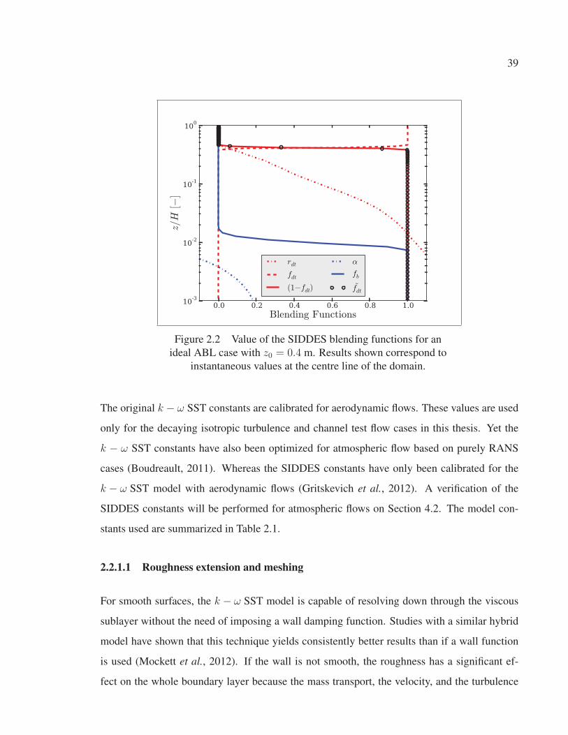
39

0.0 0.2 0.4 0.6 0.8 1.0

Blending Functions

10-3

10-2

10-1

100

z/H

[−]

rdt

fdt

(1−fdt)

α

fb

˜fdt

Figure 2.2 Value of the SIDDES blending functions for an

ideal ABL case with z0 = 0.4 m. Results shown correspond to

instantaneous values at the centre line of the domain.

The original k − ω SST constants are calibrated for aerodynamic flows. These values are used

only for the decaying isotropic turbulence and channel test flow cases in this thesis. Yet the

k − ω SST constants have also been optimized for atmospheric flow based on purely RANS

cases (Boudreault, 2011). Whereas the SIDDES constants have only been calibrated for the

k − ω SST model with aerodynamic flows (Gritskevich et al., 2012). A verification of the

SIDDES constants will be performed for atmospheric flows on Section 4.2. The model con-

stants used are summarized in Table 2.1.

2.2.1.1 Roughness extension and meshing

For smooth surfaces, the k − ω SST model is capable of resolving down through the viscous

sublayer without the need of imposing a wall damping function. Studies with a similar hybrid

model have shown that this technique yields consistently better results than if a wall function

is used (Mockett et al., 2012). If the wall is not smooth, the roughness has a significant ef-

fect on the whole boundary layer because the mass transport, the velocity, and the turbulence

40

characteristics in the near-wall region are altered (Patel, 1998). Most turbulence models, like

the RANS k − ε, require certain modifications or extra terms inserted into the original equa-

tions, or the use of wall functions to properly deal with surface roughness. On the contrary, the

k − ω SST model is capable of accurately describe the effect of a rough surface without any

modifications to the original equations (Patel and Yoon, 1996).

The roughness effect for the k − ω SST model is simply taken into account through the wall

boundary conditions. Thus, in this analysis the values of kw and ωw are based on the roughness

extension proposed by Knopp et al. (2009). This roughness extension yields successful results

for smooth (k+s < 2.25), transitional (2.25 ≤ k+

s < 90) and rough (k+s ≥ 90) surfaces (Blocken

et al., 2007). Here ks represents the equivalent sand grain roughness height, thus, k+s = ksu∗/ν.

The turbulent kinetic energy at the wall for any type of surface is then specified by

kw = φr1krough (2.25)

where

φr1 = min

(1,

k+s

90

), krough ≡ u2

∗√β∗

. (2.26)

Also u∗ represents the friction velocity which is calculated based on the streamwise velocity

gradient normal to the surface, therefore u∗ = (ν + νt)(∂u/∂n) (Knopp et al., 2009). In a

similar manner, the specific dissipation rate at the wall is

ωw = min

(u∗√β∗κ z0

,60ν

β1z21

). (2.27)

Here, z0 = φr20.03ks, and z1 denotes the distance between the wall and the centre of the first

cell (Knopp et al., 2009). Finally the blending function φr2 is given by

φr2 = min

[1,

(k+s

30

) 23

]min

[1,

(k+s

45

) 13

]min

[1,

(k+s

60

) 14

]. (2.28)

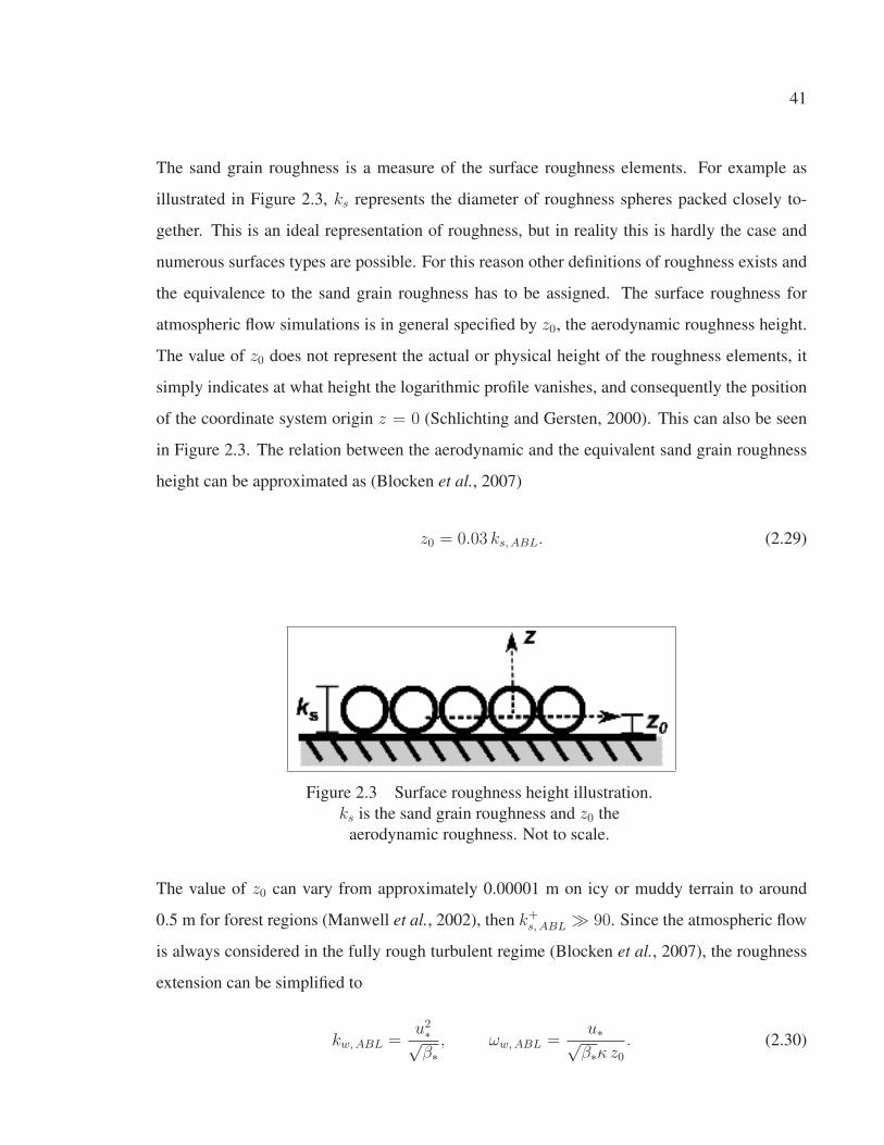
41

The sand grain roughness is a measure of the surface roughness elements. For example as

illustrated in Figure 2.3, ks represents the diameter of roughness spheres packed closely to-

gether. This is an ideal representation of roughness, but in reality this is hardly the case and

numerous surfaces types are possible. For this reason other definitions of roughness exists and

the equivalence to the sand grain roughness has to be assigned. The surface roughness for

atmospheric flow simulations is in general specified by z0, the aerodynamic roughness height.

The value of z0 does not represent the actual or physical height of the roughness elements, it

simply indicates at what height the logarithmic profile vanishes, and consequently the position

of the coordinate system origin z = 0 (Schlichting and Gersten, 2000). This can also be seen

in Figure 2.3. The relation between the aerodynamic and the equivalent sand grain roughness

height can be approximated as (Blocken et al., 2007)

z0 = 0.03 ks,ABL. (2.29)

Figure 2.3 Surface roughness height illustration.

ks is the sand grain roughness and z0 the

aerodynamic roughness. Not to scale.

The value of z0 can vary from approximately 0.00001 m on icy or muddy terrain to around

0.5 m for forest regions (Manwell et al., 2002), then k+s,ABL 90. Since the atmospheric flow

is always considered in the fully rough turbulent regime (Blocken et al., 2007), the roughness

extension can be simplified to

kw,ABL =u2∗√β∗

, ωw,ABL =u∗√β∗κ z0

. (2.30)

42

It is true that these boundary values assume a logarithmic velocity profile, thus they are in fact

based on flat terrain assumptions. However contrary to most common wall functions, kw and

ωw will only constrain the eddy-viscosity value required to solve the momentum equation at

the wall, they will not impose the wall velocity (or shear stress). Additionally, kw and ωw are

calculated based on the local and instantaneous u∗. This allows the better representation of

the unsteady local flow behaviour. Therefore, the k − ω SST-SIDDES wall treatment might be

less dependent on flat terrain assumptions than most commonly used wall functions.

As previously mentioned, the use of wall functions can be avoided for the k − ω SST model,

nevertheless it has been shown that a fine vertical grid refinement is needed for accurate re-

sults. The employed roughness extension requires the first cell centre to be located at a non-

dimensional distance of z+1 = u∗z1/ν ≈ 0.3 regardless of the roughness (Knopp et al., 2009).

This may represent a major drawback of the turbulence model, especially for high Reynolds

number flows, since extremely fine meshes are needed. Furthermore within the current compu-

tational limitations, this demanding vertical grid refinement together with the relatively large

simulation domains required to include the most energetic ABL eddies will most probably yield

near-wall cells with a rather big aspect ratio. Complex topography meshes might represent a

rather important challenge.

The modelling of a rough surface requires special attention. The flow behaviour computed

at heights below the equivalent sand grain roughness is not entirely realistic (Patel, 1998).

Therefore the simulations results for regions were z+ < k+s are not meaningful and should be

neglected. For wind blowing over a rough surface of z0 = 0.4 m, the value of the sand grain

roughness corresponds to k+s ≈ 105. Then if the roughness extension mesh requirements are

met, z+1 k+s . This type of mesh can be considered a waste of computer resources since a

rather large number of grid cells within the roughness height have to be computed and they

give no relevant information about the physics of the flow. Nevertheless, the k − ω SST rough

surface treatment does not rely on a wall function which may fail on complex and separated

flows. Consequently, this RANS turbulence model (or any hybrid model based on it) may be

43

more appropriate for modelling complex flows (Patel, 1998) and a good candidates to simulate

the ABL in complex terrain.

On the other hand, the atmospheric flow is an extreme case that has a high Reynolds number

with a roughness height which is most likely always larger that the viscous scale δν = ν/u∗.

In this situation, the drag caused by the rough surface is mainly due to pressure forces and

not due to viscous stresses (Pope, 2000). Thus the viscosity should not be relevant when

defining the height of the first node for high Reynolds flows. In wind energy simulations, it

is a common practice to set the height of the first cell centre to at least the roughness height

z0 (Blocken et al., 2007). In other words, z1 is determined by a non-dimensional outer scale

ζ+1 = z1/z0 ≥ 1.0. Following these mesh guideline makes the simulations considerably less

computational demanding, but it does not satisfy the roughness extension requirements. For

example, a z1 computed based on an outer scale will correspond to an inner scale value of

z+1 ≈ 104 for ABL flows (assuming z0 = 0.4 m). Some other examples are given in Table 2.2.

The impact that the value of z1 has on the simulations results will be analyzed in more detail

for ABL flows in Section 4.2.1 (Figure 4.9).

Table 2.2 Examples of z1 values

Definition of z1 based on: z0 [m] z1 [m]

0.0002 3.8 · 10−5

z+1 = u∗z1/ν = 1 0.03 3.8 · 10−5

(u∗ = 0.3880 m/s and ν = 1.5 · 10−5 m2/s) 0.4 3.8 · 10−5

0.0002 0.0002

ζ+1 = z1/z0 = 1 0.03 0.03

0.4 0.4

2.3 Summary and subsequent tasks

The basic concepts of CFD have been explained within the OpenFOAM framework and within

the microscale atmospheric modelling context. Furthermore, a hybrid model to undertake mi-

croscale simulations has been proposed and described in detail. The k − ω SST-SIDDES hy-

44

brid model is considered a good candidate for microscale simulations for the atmospheric flow

because of two main reasons: its particular wall treatment is less dependent on flat terrain as-

sumptions, and it could provide a good compromise between the higher accuracy and lower

computer cost.

The k − ω SST model has rarely been used to model the ABL at a microscale level; while the

SIDDES technique have never been utilized outside of aerodynamic flow studies. The possibil-

ity of avoiding the standard wall functions and the simpler roughness treatment provided by the

k − ω SST, together with the LLM correction and probable computing time reduction (com-

pared to a standard LES) offered by the SIDDES make this hybrid model a potential candidate

for ABL simulations. To this end, a rigorous validation of the proposed hybrid model is per-

formed using some well-known canonical flows. This process will yield valuable information

about the advantages and inherent limitations of the turbulence model, as well as to explain

certain modelling concepts often overlook in the literature. Consequently, the model validation

will set solid bases to understand the flow behaviour computed by atmospheric simulations.

CHAPTER 3

TURBULENCE MODEL VALIDATION ON CANONICAL FLOWS

The k − ω SST-SIDDES model is carefully validated on canonical flows in this chapter. First,

the LES behaviour of this hybrid turbulence model is compared against a well validated DNS

of decaying turbulence. The objective is to test if the model can reproduce the transfer of

energy between the different turbulent scales. Then, a homogeneous shear flow was simulated

to study how the model behaves in the presence of rotation and mean shear. Finally, the half

channel flow is analyzed to investigate the URANS and LES behaviour due to the presence

of a wall. Additionally, the half channel test cases are analyzed for rather high Reynolds and

extremely rough surfaces such as the ones required in atmospheric flows.

3.1 Decaying isotropic turbulence flow

Decaying isotropic turbulence (DIT) is the most simple and fundamental turbulent flow1. It

is an unbounded flow characterized by the absence of mean velocity gradients, so there is no

turbulence production or shear stresses. As a result, the turbulence merely decays over time.

The time evolution of the total turbulent kinetic energy (i.e. filtered plus modelled) is simply

equal to the total dissipation, thus

dktotaldt

= −εtotal. (3.1)

Decaying isotropic turbulence is an ideal and theoretical flow, but it can be fairly well approx-

imated by a grid turbulence experiment (Comte-Bellot and Corrsin, 1971). This experiment

consist of a flow with a streamwise velocity U0 which encounters a grid. Behind this grid,

on the laboratory frame the turbulence decays in x, the direction of the flow. However, on

an inertial frame moving at U0 the turbulence statistics evolve over time as t = x/U0 (Pope,

2000). Based on the Taylor hypothesis the time-evolving velocity fluctuations of a DIT can

1In the literature it is sometimes referred as homogeneous isotropic turbulence (HIT) (Sagaut and Cambon,

2008).

46

be interpreted as a frozen flow field advected by the uniform steady flow of the experiment.

Mathematically this means (Sagaut and Cambon, 2008)

[u(x, t)]DIT = [u(x− U0t, 0)]Exp. (3.2)

The decaying turbulence processes are not completely understood, nevertheless this flow has

been studied extensively and it is well documented. Numerically, DIT is used as benchmark

to test the transfer of kinetic energy between the different turbulent scales in LES models,

as well as in the LES mode of a hybrid model. A DIT case modelled using a DES approach

should not present any URANS regions since there are no solid surfaces. Therefore all the DES

approaches should have l = lLES and compute identical results. However to properly model a

DIT case using IDDES and SIDDES, the LES mode has to be enforced. The reason for this is

that the definition of the ΔIDDES is based on a distance to a non existing surface. In this case,

OpenFOAM erroneously yields ΔIDDES = Cwhmax, underestimating the lengthscale. To force

the LES mode in the DIT case, the value of the constant Cw was set to a high enough value

that will trigger the correct filter width (i.e. ΔIDDES = hmax) and consequently the proper

lengthscale.

Most importantly the DIT flow case is crucial to calibrate the model constant

CDES = CDES(Ck−ε, Ck−ω) within the specific numerical framework (i.e. interpolation

schemes, software, etc.) (Bunge et al., 2007). The k − ω SST-DES has been calibrated pre-

viously for a different numerical framework (Travin et al., 2002), thus those constants were

taken as a initial reference to calibrate the proposed model implementation in OpenFOAM

(refer to SIDDES constants in Table I-1). Those constants will be adjusted later if needed.

The LES mode of the k − ω SST-DES and k − ω SST-SIDDES will be validated against the

well-known Comte-Bellot and Corrsin’s grid turbulence experiments at a Reynolds number of

Reλ = urmsλ/ν ≈ 70 (Comte-Bellot and Corrsin, 1971), and against Wray’s DNS results at

47

Reλ ≈ 945− 58 (Jimenez J. (Ed.), 1997). The Taylor microscale is defined as

λ = 15νu2rms/εtotal, (3.3)

where urms is the rms velocity, and the total dissipation εtotal is the sum of the filtered ε and

subgrid ε contributions. The simulations were performed in a cubic domain of size L = 2π

and periodic boundaries. The transport and turbulence model equations were discretized us-

ing a second-order central interpolation scheme for the divergence terms (unless otherwise

noticed), while a backward second-order implicit scheme was used for the time derivative

term. The pressure-implicit split-operator (PISO) algorithm was used for the velocity-pressure

coupling (Issa, 1985). A maximum Courant-Friedrichs-Lewy (CFL) number of 0.1 and the

aerodynamic constants from Table I-1 were imposed.

Starting the simulation with a realistic turbulent field prove to be extremely crucial. For this

reason the velocity field was initialized using the DNS data set provided by A. Wray in the

AGARD database (Jimenez J. (Ed.), 1997) for a 1283 mesh with a Reλ ∼ 104. This field was

projected on physical space for the coarser meshes. Unfortunately, at those Reλ the inertial

range slope of −5/3 is not distinguished as clearly as it does for higher Reynolds number. To

generate the proper initial fields for k, ω and specially νt, a simulation of the "frozen” initial

velocity field was carried out following the work of Bunge et al. (2007). This computation

solves only the steady turbulence model equations without solving for the velocity and pres-

sure. The converged simulation yields the initial fields of all the variables which are consistent

with the given velocity field. The "frozen" turbulence technique is not needed for other models

like Smagorinsky because the νt field is calculated directly from the velocity field, but this is

not the case for the DES approaches. Finally, this robust initial turbulent field is let to decay

freely. Figure 3.1 depicts the time evolution of the vorticity field.

The total turbulent kinetic energy ktotal should decay as a power-law in the DIT case. Hence,

ktotal(t) = k0

(t

t0

)−n

. (3.4)

48

(a) t∗ = 0.0 (b) t∗ = 2.0 (c) t∗ = 5.0

Figure 3.1 Vorticity contours at different non-dimensional times for the DIT 643

case. The contour levels are the same in all figures and are colour by the magnitude

of the velocity (Units: [m/s]).

Consequently, the dissipation should behave as εtotal ∼ t−(n+1) and the integral scale as

L ∼ t(1+n/2) (Pope, 2000). The turbulent nonlinear effects are more predominant when Reλ is

high, as Reλ decreases the inertial effects become negligible and the viscous linear effects dom-

inate. For this reason, two different decaying regimes could be distinguished (Sagaut and Cam-

bon, 2008). For the first regime, the decay coefficient measured by several experiments falls

in the range of 6/5 ≤ n ≤ 4/3 (Sagaut and Cambon, 2008), while simulations have yield

n = 1.25 (Kang et al., 2003). On the other hand the decay rate for the second regime increases

up to n ∼ 2.0 − 2.5 (Sagaut and Cambon, 2008; Pope, 2000). To this day, it is still extremely

difficult to achieve the second regime in experiments and in simulations due to the extremely

low Reynolds numbers involved (Sagaut and Cambon, 2008). Therefore no much details about

this second regime are available in the literature. Hence, this validation test will only focus on

the first decay regime.

Figure 3.2 gives the turbulent kinetic energy decay. The results show a volume average, hence

ktotal =∑

i(ktotal, i ∗Δvi)/Vtotal. The decaying rate is practically the same for DES and SID-

DES as expected, and consistent with the Smagorinsky model. Additionally, the calculated

value of n is approximately 1.25 using a 323 mesh, which agrees with the literature and with

the DNS data also provided in the AGARD database (Jimenez J. (Ed.), 1997). Simulations with

1283 cells and 643 cells yield consistent results as Figure 3.3 demonstrates. A decay exponent

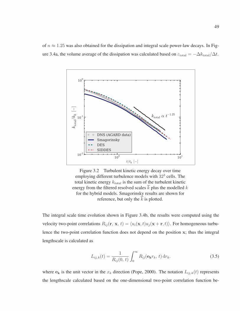
49

of n ≈ 1.25 was also obtained for the dissipation and integral scale power-law decays. In Fig-

ure 3.4a, the volume average of the dissipation was calculated based on εtotal = −Δktotal/Δt.

100

101

t/t0 [−]

10-2

10-1

100

kto

tal/k0

[−]

ktotal α t−1.25

DNS (AGARD data)

Smagorinsky

DES

SIDDES

Figure 3.2 Turbulent kinetic energy decay over time

employing different turbulence models with 323 cells. The

total kinetic energy ktotal is the sum of the turbulent kinetic

energy from the filtered resolved scales k plus the modelled kfor the hybrid models. Smagorinsky results are shown for

reference, but only the k is plotted.

The integral scale time evolution shown in Figure 3.4b, the results were computed using the

velocity two-point correlations Rij(r, x, t) = 〈ui(x, t)uj(x+ r, t)〉. For homogeneous turbu-

lence the two-point correlation function does not depend on the position x; thus the integral

lengthscale is calculated as

Lij, k(t) =1

Rij(0, t)

∫ ∞

0

Rij(ekrk, t) drk. (3.5)

where ek is the unit vector in the xk direction (Pope, 2000). The notation Lij, k(t) represents

the lengthscale calculated based on the one-dimensional two-point correlation function be-

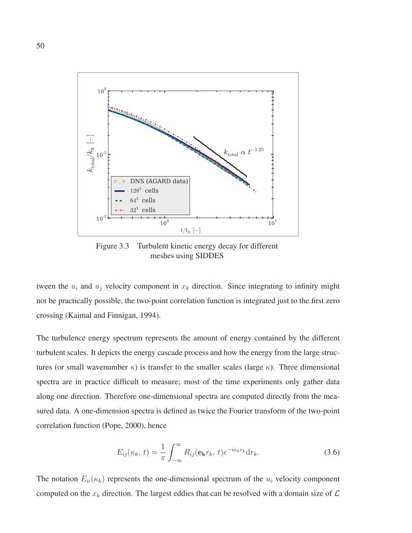
50

100

101

t/t0 [−]

10-2

10-1

100

ktotal/k0[−

]

ktotal α t−1.25

DNS (AGARD data)

1283 cells

643 cells

323 cells

Figure 3.3 Turbulent kinetic energy decay for different

meshes using SIDDES

tween the ui and uj velocity component in xk direction. Since integrating to infinity might

not be practically possible, the two-point correlation function is integrated just to the first zero

crossing (Kaimal and Finnigan, 1994).

The turbulence energy spectrum represents the amount of energy contained by the different

turbulent scales. It depicts the energy cascade process and how the energy from the large struc-

tures (or small wavenumber κ) is transfer to the smaller scales (large κ). Three dimensional

spectra are in practice difficult to measure; most of the time experiments only gather data

along one direction. Therefore one-dimensional spectra are computed directly from the mea-

sured data. A one-dimension spectra is defined as twice the Fourier transform of the two-point

correlation function (Pope, 2000), hence

Eij(κk, t) =1

π

∫ ∞

−∞Rij(ekrk, t)e

−iκkrkdrk. (3.6)

The notation Eii(κk) represents the one-dimensional spectrum of the ui velocity component

computed on the xk direction. The largest eddies that can be resolved with a domain size of L

51

100

101

t/t0 [−]

10-2

10-1

100

ε total/ε 0

[−]

εtotal α t−(1.00+1.25)

DNS (AGARD data)

1283 cells

643 cells

323 cells

(a) ε decay

100

101

t/t0 [−]

10-1

100

L11,1/L

0[−

]

L α t 1.00−1.25/2.00

DNS (AGARD data)

323 cells

(b) L11,1 decay

Figure 3.4 Time evolution using k − ω SST-SIDDES compared against the results

provided in the AGARD database (Jimenez J. (Ed.), 1997).

have a wavenumber of κmin = 2π/L. On the other hand, the smallest eddies that can be theoret-

ically resolved depend on the grid resolution Δ and the Nyquist theorem; hence κmax = π/Δ.

Figure 3.5 shows the one-dimensional spectra computed with the k − ω SST-SIDDES model

compared to the DNS one-dimensional spectra computed by Wray. The hybrid model spec-

tra are estimated based on the Welch method (Welch, 1967). The hybrid model reproduces

fairly well the spectrum slope in the inertial range, as well as the time evolution of such energy

spectra. However it can be seen that the non-dimensional longitudinal spectra E∗11(κ

∗1) do not

perfectly match the DNS results at smaller wavenumbers. This discrepancy diminishes over

time. A small cusp is visible at high wavenumbers, this phenomenon is well known for eddy

viscosity models (Lesieur and Métais, 1996). Additionally in Figure 3.6 it can be observed that

E∗ii(κ

∗i ) ≈ 3/4E∗

jj(κ∗i ) as expected for the inertial range dynamics of an isotropic turbulent

field (Pope, 2000).

The spectra normalized by the Kolmogorov scale η are given in Figure 3.7. The non-

dimensional longitudinal energy spectra from the hybrid model computations compare well

with the grid turbulence experiments and DNS results. As expected the k − ω SST-DES

and k − ω SST-SIDDES results are equivalent. The mentioned small cusp is visible at high

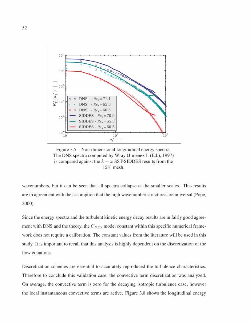
52

100

101

102

κ∗

1 [−]

10-6

10-5

10-4

10-3

10-2

10-1

E∗ 11(κ

∗ 1)

[−]

DNS - Reλ=71.1

DNS - Reλ=65.3

DNS - Reλ=60.5

SIDDES - Reλ=70.9

SIDDES - Reλ=65.3

SIDDES - Reλ=60.5

Figure 3.5 Non-dimensional longitudinal energy spectra.

The DNS spectra computed by Wray (Jimenez J. (Ed.), 1997)

is compared against the k − ω SST-SIDDES results from the

1283 mesh.

wavenumbers, but it can be seen that all spectra collapse at the smaller scales. This results

are in agreement with the assumption that the high wavenumber structures are universal (Pope,

2000).

Since the energy spectra and the turbulent kinetic energy decay results are in fairly good agree-

ment with DNS and the theory, the CDES model constant within this specific numerical frame-

work does not require a calibration. The constant values from the literature will be used in this

study. It is important to recall that this analysis is highly dependent on the discretization of the

flow equations.

Discretization schemes are essential to accurately reproduced the turbulence characteristics.

Therefore to conclude this validation case, the convective term discretization was analyzed.

On average, the convective term is zero for the decaying isotropic turbulence case, however

the local instantaneous convective terms are active. Figure 3.8 shows the longitudinal energy

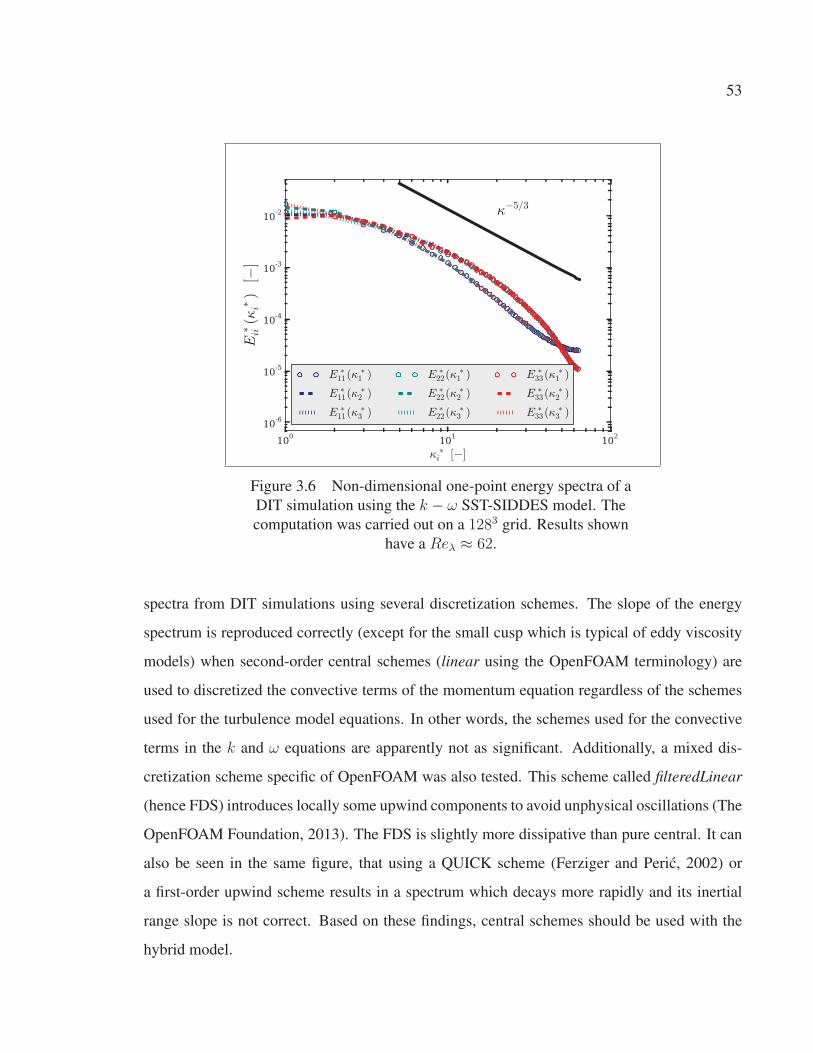
53

100

101

102

κ ∗

i [−]

10-6

10-5

10-4

10-3

10-2

E∗ ii(κ

∗ i)

[−]

κ−5/3

E ∗

11(κ∗

1 )

E ∗

11(κ∗

2 )

E ∗

11(κ∗

3 )

E ∗

22(κ∗

1 )

E ∗

22(κ∗

2 )

E ∗

22(κ∗

3 )

E ∗

33(κ∗

1 )

E ∗

33(κ∗

2 )

E ∗

33(κ∗

3 )

Figure 3.6 Non-dimensional one-point energy spectra of a

DIT simulation using the k − ω SST-SIDDES model. The

computation was carried out on a 1283 grid. Results shown

have a Reλ ≈ 62.

spectra from DIT simulations using several discretization schemes. The slope of the energy

spectrum is reproduced correctly (except for the small cusp which is typical of eddy viscosity

models) when second-order central schemes (linear using the OpenFOAM terminology) are

used to discretized the convective terms of the momentum equation regardless of the schemes

used for the turbulence model equations. In other words, the schemes used for the convective

terms in the k and ω equations are apparently not as significant. Additionally, a mixed dis-

cretization scheme specific of OpenFOAM was also tested. This scheme called filteredLinear

(hence FDS) introduces locally some upwind components to avoid unphysical oscillations (The

OpenFOAM Foundation, 2013). The FDS is slightly more dissipative than pure central. It can

also be seen in the same figure, that using a QUICK scheme (Ferziger and Peric, 2002) or

a first-order upwind scheme results in a spectrum which decays more rapidly and its inertial

range slope is not correct. Based on these findings, central schemes should be used with the

hybrid model.

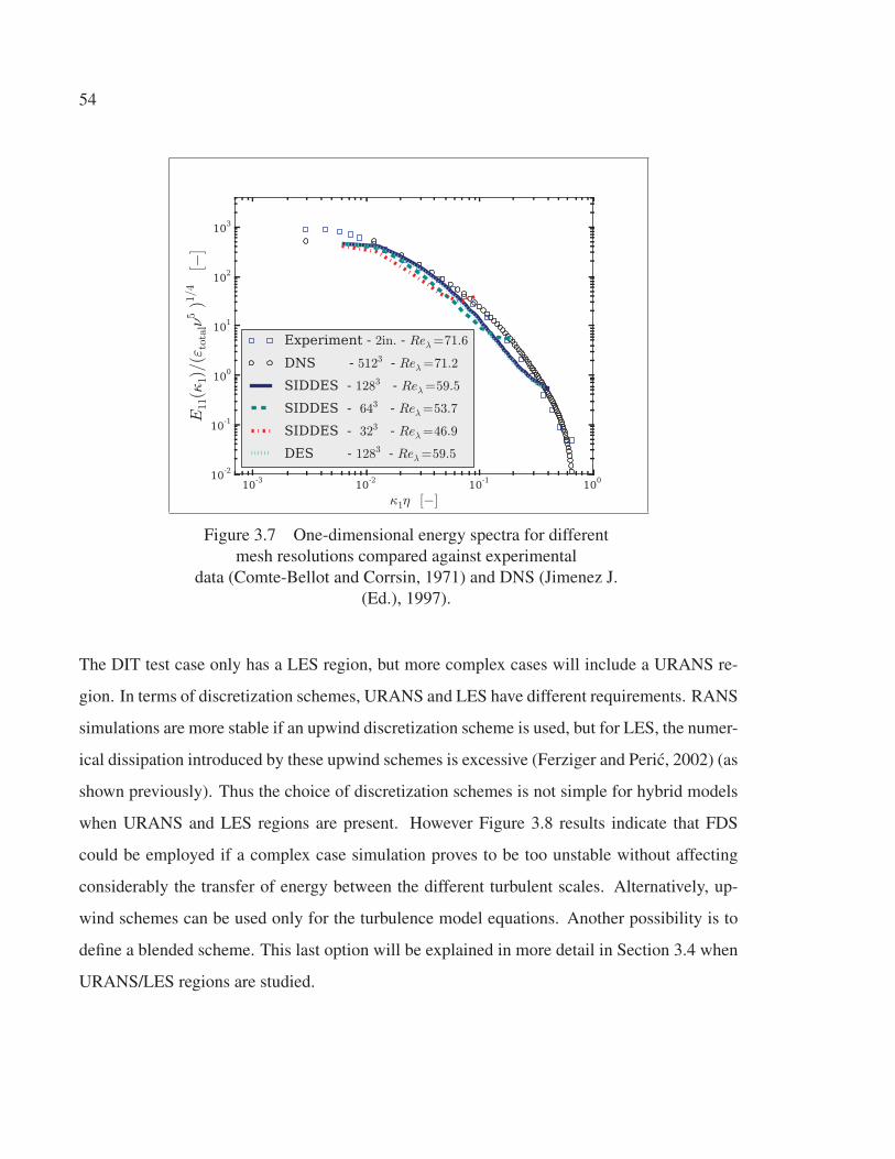
54

10-3

10-2

10-1

100

κ1η [−]

10-2

10-1

100

101

102

103

E11(κ

1)/(ε

totalν

5)1/4

[−]

Experiment - 2in. - Reλ=71.6

DNS - 5123 - Reλ=71.2

SIDDES - 1283 - Reλ=59.5

SIDDES - 643 - Reλ=53.7

SIDDES - 323 - Reλ=46.9

DES - 1283 - Reλ=59.5

Figure 3.7 One-dimensional energy spectra for different

mesh resolutions compared against experimental

data (Comte-Bellot and Corrsin, 1971) and DNS (Jimenez J.

(Ed.), 1997).

The DIT test case only has a LES region, but more complex cases will include a URANS re-

gion. In terms of discretization schemes, URANS and LES have different requirements. RANS

simulations are more stable if an upwind discretization scheme is used, but for LES, the numer-

ical dissipation introduced by these upwind schemes is excessive (Ferziger and Peric, 2002) (as

shown previously). Thus the choice of discretization schemes is not simple for hybrid models

when URANS and LES regions are present. However Figure 3.8 results indicate that FDS

could be employed if a complex case simulation proves to be too unstable without affecting

considerably the transfer of energy between the different turbulent scales. Alternatively, up-

wind schemes can be used only for the turbulence model equations. Another possibility is to

define a blended scheme. This last option will be explained in more detail in Section 3.4 when

URANS/LES regions are studied.

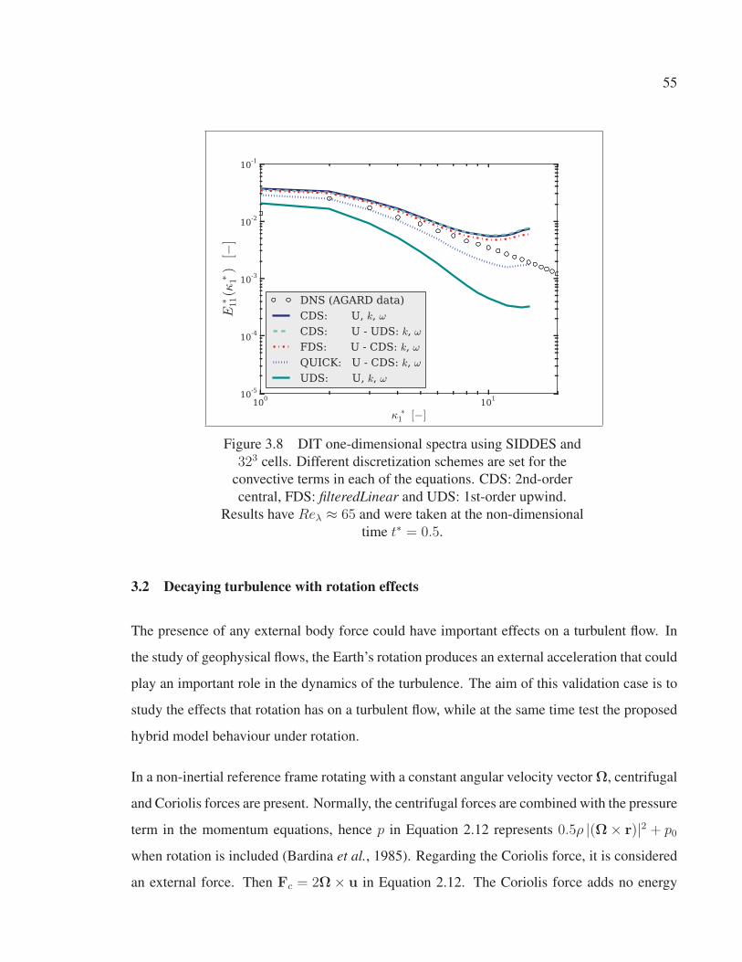
55

100

101

κ∗

1 [−]

10-5

10-4

10-3

10-2

10-1

E∗ 11(κ

∗ 1)

[−]

DNS (AGARD data)

CDS: U, k, ω

CDS: U - UDS: k, ω

FDS: U - CDS: k, ω

QUICK: U - CDS: k, ω

UDS: U, k, ω

Figure 3.8 DIT one-dimensional spectra using SIDDES and

323 cells. Different discretization schemes are set for the

convective terms in each of the equations. CDS: 2nd-order

central, FDS: filteredLinear and UDS: 1st-order upwind.

Results have Reλ ≈ 65 and were taken at the non-dimensional

time t∗ = 0.5.

3.2 Decaying turbulence with rotation effects

The presence of any external body force could have important effects on a turbulent flow. In

the study of geophysical flows, the Earth’s rotation produces an external acceleration that could

play an important role in the dynamics of the turbulence. The aim of this validation case is to

study the effects that rotation has on a turbulent flow, while at the same time test the proposed

hybrid model behaviour under rotation.

In a non-inertial reference frame rotating with a constant angular velocity vector Ω, centrifugal

and Coriolis forces are present. Normally, the centrifugal forces are combined with the pressure

term in the momentum equations, hence p in Equation 2.12 represents 0.5ρ |(Ω× r)|2 + p0

when rotation is included (Bardina et al., 1985). Regarding the Coriolis force, it is considered

an external force. Then Fc = 2Ω× u in Equation 2.12. The Coriolis force adds no energy

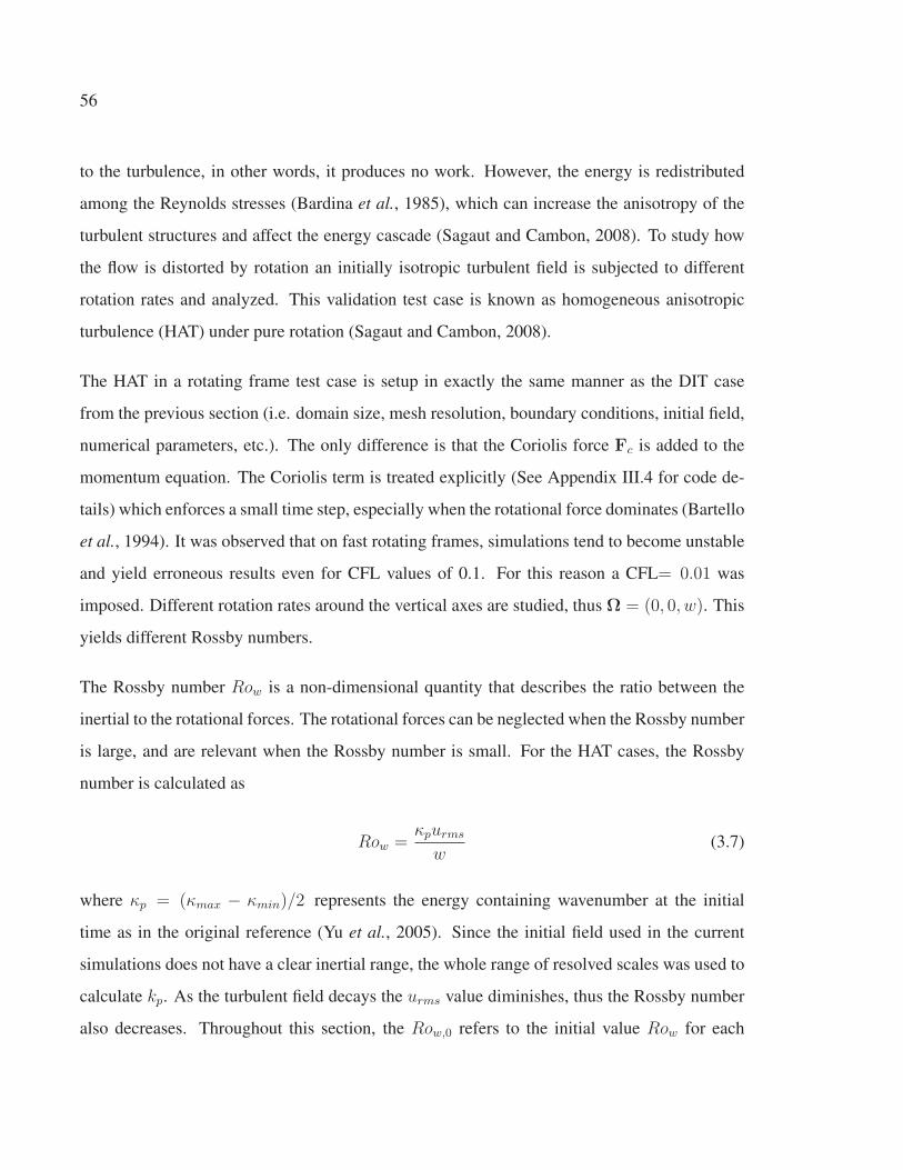
56

to the turbulence, in other words, it produces no work. However, the energy is redistributed

among the Reynolds stresses (Bardina et al., 1985), which can increase the anisotropy of the

turbulent structures and affect the energy cascade (Sagaut and Cambon, 2008). To study how

the flow is distorted by rotation an initially isotropic turbulent field is subjected to different

rotation rates and analyzed. This validation test case is known as homogeneous anisotropic

turbulence (HAT) under pure rotation (Sagaut and Cambon, 2008).

The HAT in a rotating frame test case is setup in exactly the same manner as the DIT case

from the previous section (i.e. domain size, mesh resolution, boundary conditions, initial field,

numerical parameters, etc.). The only difference is that the Coriolis force Fc is added to the

momentum equation. The Coriolis term is treated explicitly (See Appendix III.4 for code de-

tails) which enforces a small time step, especially when the rotational force dominates (Bartello

et al., 1994). It was observed that on fast rotating frames, simulations tend to become unstable

and yield erroneous results even for CFL values of 0.1. For this reason a CFL= 0.01 was

imposed. Different rotation rates around the vertical axes are studied, thus Ω = (0, 0, w). This

yields different Rossby numbers.

The Rossby number Row is a non-dimensional quantity that describes the ratio between the

inertial to the rotational forces. The rotational forces can be neglected when the Rossby number

is large, and are relevant when the Rossby number is small. For the HAT cases, the Rossby

number is calculated as

Row =κpurms

w(3.7)

where κp = (κmax − κmin)/2 represents the energy containing wavenumber at the initial

time as in the original reference (Yu et al., 2005). Since the initial field used in the current

simulations does not have a clear inertial range, the whole range of resolved scales was used to

calculate kp. As the turbulent field decays the urms value diminishes, thus the Rossby number

also decreases. Throughout this section, the Row,0 refers to the initial value Row for each

57

simulation. Its it important to mention that the Rossby number RoL used for atmospheric flow

cases is defined differently; it is based on the large scales (See Section 4.2.2).

As the Coriolis force does not generate energy, the initial unbounded isotropic turbulent field

subjected to rotation will also decay. Nevertheless, the energy decay rate decreases as the

Row,0 increases (Bardina et al., 1985). This can be seen in Figure 3.9. Simulations with

initially isotropic turbulent fields that are subjected to the Earth’s rotation rate do not show any

significant difference from the freely DIT case (Row,0 = ∞). This effect is also negligible

even when the inertial forces are fifty times greater that the rotational forces, Row,0 = 50. The

simulations for an initial Row,0 = 1 start to become unstable; this is probably because the time

step is not small enough as explained previously. To emphasize the effect that rotation has on

the decay rate, the spectra for different angular velocities is given in Figure 3.10. As Yu et al.

(2005), the rotation inhibits the energy cascade, and that energy tends to accumulate on the

small wavenumbers as Row,0 increases. Also, the κ−5/3 is no longer followed; in other words,

the turbulence is not described by the Kolmogorov theory.

Another important characteristic of the rotation effects on an isotropic field is the generation of

anisotropic structures. This can be observed in Figure 3.11 where the different components of

velocity are equal for high values of Row,0, but are altered as Row,0 decreases. This anisotropy

can be better perceived in the integral lengthscales for the various velocity components. For

instance, Figure 3.12 shows that for a case without rotation or with wEarth, the lengthscales

are Lii,i ≈ 2Ljj,i (i �= j) as expected for isotropic turbulent fields. This is no longer valid

for the case with initial Row,0 = 5, where the lengthscales calculated along the rotation axis

grow faster as observed by Bardina et al. (1983). This result show that the turbulent vortices

are elongated along the axis of rotation (Godeferd, 2012) and the flow tends to become two-

dimensional.

As expected, the results show that the Earth’s angular velocity has a negligible effect on the

dynamics of the turbulence for the HAT validation case. This is also valid for Row,0 = 50.

As it will be explained later in Section 4.2.2, the large scale Rossby number RoL obtained

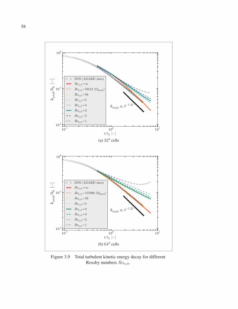
58

10-1

100

101

t/t0 [−]

10-2

10-1

100

ktotal/k0[−]

ktotal α t−1.25

DNS (AGARD data)

Row,0 =∞

Row,0 =76512 (ΩEarth)

Row,0 =56

Row,0 =5

Row,0 =4

Row,0 =3

Row,0 =2

Row,0 =1

(a) 323 cells

10-1

100

101

t/t0 [−]

10-2

10-1

100

ktotal/k0[−]

ktotal α t−1.25

DNS (AGARD data)

Row,0 =∞


Row,0 =50

Row,0 =5

Row,0 =4

Row,0 =3

Row,0 =2

Row,0 =1

(b) 643 cells

Figure 3.9 Total turbulent kinetic energy decay for different

Rossby numbers Row,0.

59

100

101

κ ∗

1 [−]

10-5

10-4

10-3

10-2

E∗ 11(κ

∗ 1)

[−]

κ−5/3

Row,0 =∞


Row,0 =50

Row,0 =5

Row,0 =4

Row,0 =3

Row,0 =2

(a) Longitudinal spectra

100

101

κ ∗

3 [−]

10-5

10-4

10-3

10-2

E∗ 11(κ

∗ 3)

[−]

κ−5/3

Row,0 =∞


Row,0 =50

Row,0 =5

Row,0 =4

Row,0 =3

Row,0 =2

(b) Vertical spectra

Figure 3.10 One-dimensional energy spectra for different

Rossby numbers taken at a non-dimensional time t∗ = 2.0 for

the 643 mesh.

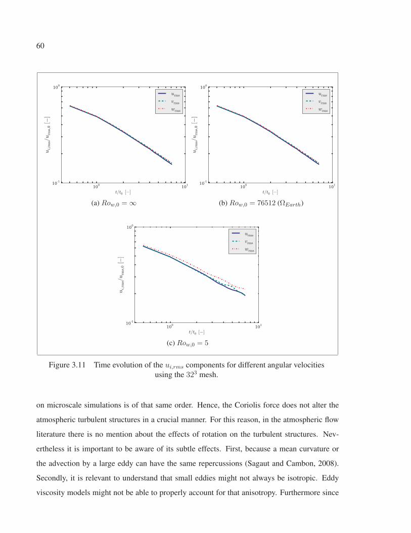
60

100

101

t/t0 [−]

10-1

100

ui,rm

s/urm

s,0[−

]

urms

vrms

wrms

(a) Row,0 = ∞

100

101

t/t0 [−]

10-1

100

ui,rm

s/urm

s,0[−

]

urms

vrms

wrms

(b) Row,0 = 76512 (ΩEarth)

100

101

t/t0 [−]

10-1

100

ui,rm

s/urm

s,0[−

]

urms

vrms

wrms

(c) Row,0 = 5

Figure 3.11 Time evolution of the ui,rms components for different angular velocities

using the 323 mesh.

on microscale simulations is of that same order. Hence, the Coriolis force does not alter the

atmospheric turbulent structures in a crucial manner. For this reason, in the atmospheric flow

literature there is no mention about the effects of rotation on the turbulent structures. Nev-

ertheless it is important to be aware of its subtle effects. First, because a mean curvature or

the advection by a large eddy can have the same repercussions (Sagaut and Cambon, 2008).

Secondly, it is relevant to understand that small eddies might not always be isotropic. Eddy

viscosity models might not be able to properly account for that anisotropy. Furthermore since

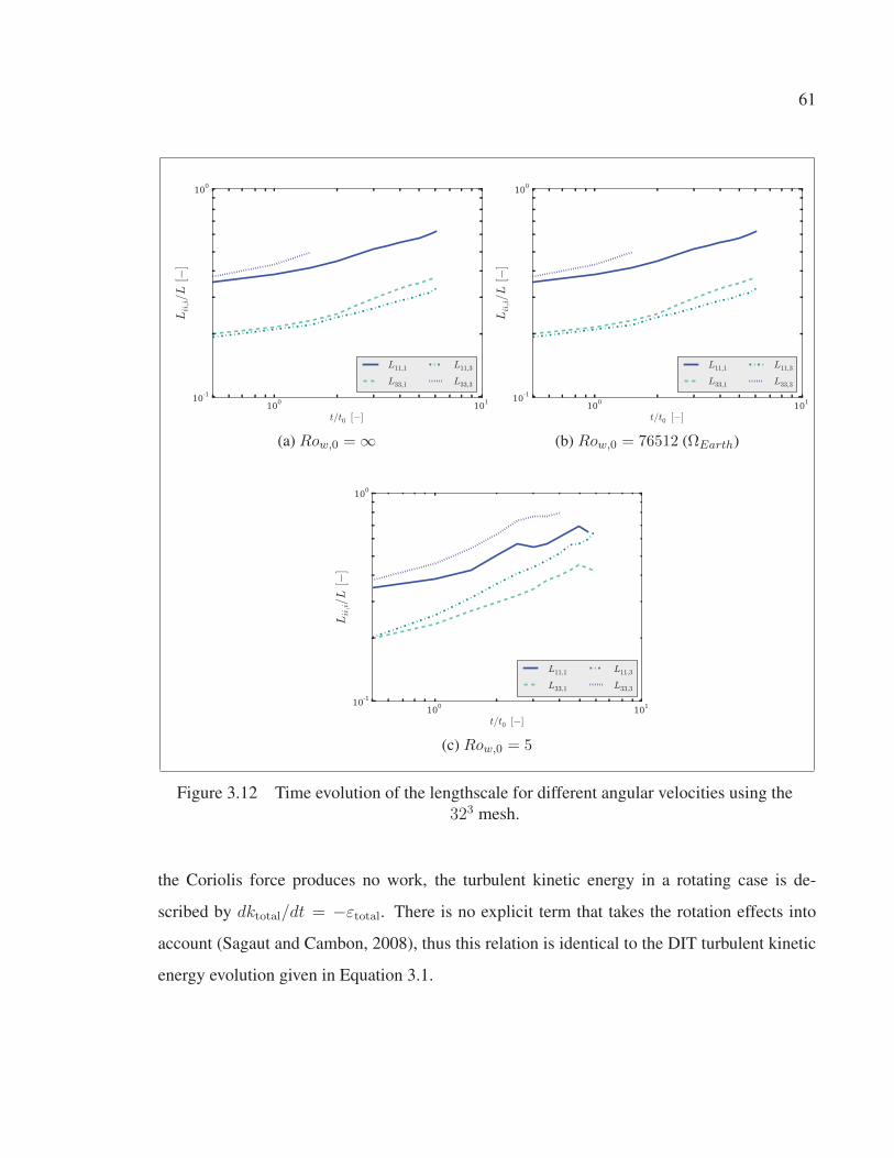
61

100

101

t/t0 [−]

10-1

100

Lii,i/L

[−]

L11,1

L33,1

L11,3

L33,3

(a) Row,0 = ∞

100

101

t/t0 [−]

10-1

100

Lii,i/L

[−]

L11,1

L33,1

L11,3

L33,3

(b) Row,0 = 76512 (ΩEarth)

100

101

t/t0 [−]

10-1

100

Lii,i/L

[−]

L11,1

L33,1

L11,3

L33,3

(c) Row,0 = 5

Figure 3.12 Time evolution of the lengthscale for different angular velocities using the

323 mesh.

the Coriolis force produces no work, the turbulent kinetic energy in a rotating case is de-

scribed by dktotal/dt = −εtotal. There is no explicit term that takes the rotation effects into

account (Sagaut and Cambon, 2008), thus this relation is identical to the DIT turbulent kinetic

energy evolution given in Equation 3.1.

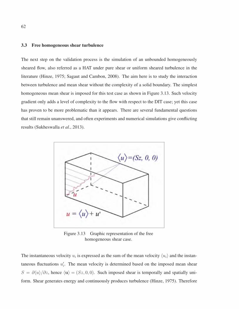
62

3.3 Free homogeneous shear turbulence

The next step on the validation process is the simulation of an unbounded homogeneously

sheared flow, also referred as a HAT under pure shear or uniform sheared turbulence in the

literature (Hinze, 1975; Sagaut and Cambon, 2008). The aim here is to study the interaction

between turbulence and mean shear without the complexity of a solid boundary. The simplest

homogeneous mean shear is imposed for this test case as shown in Figure 3.13. Such velocity

gradient only adds a level of complexity to the flow with respect to the DIT case; yet this case

has proven to be more problematic than it appears. There are several fundamental questions

that still remain unanswered, and often experiments and numerical simulations give conflicting

results (Sukheswalla et al., 2013).

Figure 3.13 Graphic representation of the free

homogeneous shear case.

The instantaneous velocity ui is expressed as the sum of the mean velocity 〈ui〉 and the instan-

taneous fluctuations u′i. The mean velocity is determined based on the imposed mean shear

S = ∂〈u〉/∂z, hence 〈u〉 = (Sz, 0, 0). Such imposed shear is temporally and spatially uni-

form. Shear generates energy and continuously produces turbulence (Hinze, 1975). Therefore

63

the turbulent kinetic energy evolves in time as

dktotaldt

= −S〈u′w′〉 − εtotal. (3.8)

Contrary to the previous validation cases, there is the energy production term P = −S〈u′w′〉in the equation (Sagaut and Cambon, 2008). A self-similar state is attained if the turbu-

lence production is compensated by the local dissipation (Davidson, 2004). Most experi-

ments (Tavoularis and Karnik, 1989) and numerical studies (Rogallo, 1981; Rogers and Moin,

1987; Lee et al., 1990) suggest that the turbulent kinetic energy in unbounded shear flows

grows exponentially in time. It has been observed that the production term equals the dis-

sipation term (P/ε ∼ 1) only when a low-shear is imposed; hence a steady state regime is

found for these cases. However high-shear cases converge to an asymptotic regime where

P/ε > 1 (Tavoularis and Karnik, 1989). It appears that the P ∼ ε balance can only be achieved

on confined cases (Pumir, 1996).

A DNS numerical study performed by Lee et al. (1990) was chosen to validate the

k − ω SST-SIDDES hybrid model. The results of this test case are also available on the

AGARD database (Jimenez J. (Ed.), 1997). In this case, the unbounded computational do-

main consists of a periodic box and an initial isotropic field which is subjected to a high mean

shear. The hybrid model will yield only LES regions due to the absence of solid walls. The

domain size is (Lx, Ly, Lz) = (8π, 2π, 2π). It is larger in the streamwise direction to allow for

the elongated turbulent scales that will developed due to the shearing action. The SIDDES

mesh has (128× 32× 32) cells while the referenced DNS have four times more cells in each

direction. A shear of S = 10 (with units of 1/time) is defined as well. The initial field was gen-

erated based on the DNS data set provided by A. Wray (Jimenez J. (Ed.), 1997) for DIT cases.

This data set was concatenated four times in the streamwise direction and then mapped to the

shear flow mesh. Subsequently it was let to decay freely until the required initial Reλ ∼ 50

was attained. Once a mean shear is imposed, the velocity field is no longer periodic in the verti-

cal direction. Consequently to simulate this unbounded computational box, the flow equations

have to be slightly rearranged.

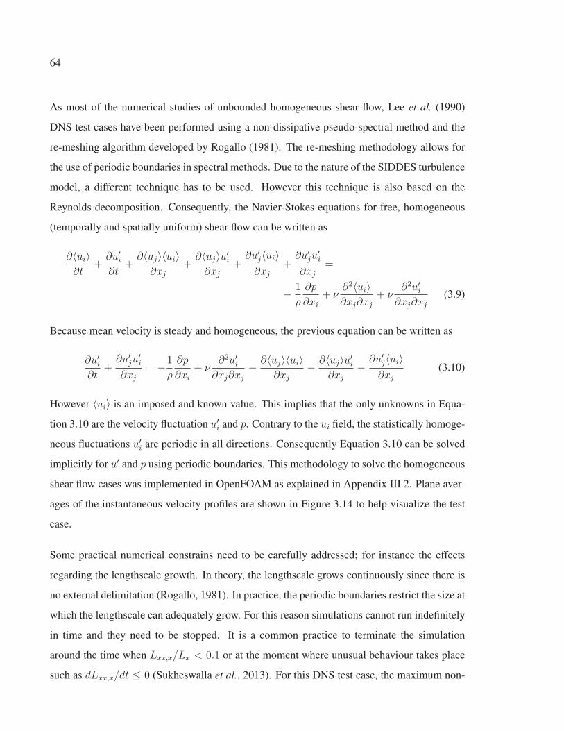
64

As most of the numerical studies of unbounded homogeneous shear flow, Lee et al. (1990)

DNS test cases have been performed using a non-dissipative pseudo-spectral method and the

re-meshing algorithm developed by Rogallo (1981). The re-meshing methodology allows for

the use of periodic boundaries in spectral methods. Due to the nature of the SIDDES turbulence

model, a different technique has to be used. However this technique is also based on the

Reynolds decomposition. Consequently, the Navier-Stokes equations for free, homogeneous

(temporally and spatially uniform) shear flow can be written as

∂〈ui〉∂t

+∂u′

i

∂t+

∂〈uj〉〈ui〉∂xj

+∂〈uj〉u′

i

∂xj

+∂u′

j〈ui〉∂xj

+∂u′

ju′i

∂xj

=

− 1

ρ

∂p

∂xi

+ ν∂2〈ui〉∂xj∂xj

+ ν∂2u′

i

∂xj∂xj

(3.9)

Because mean velocity is steady and homogeneous, the previous equation can be written as

∂u′i

∂t+

∂u′ju

′i

∂xj

= −1

ρ

∂p

∂xi

+ ν∂2u′

i

∂xj∂xj

− ∂〈uj〉〈ui〉∂xj

− ∂〈uj〉u′i

∂xj

− ∂u′j〈ui〉∂xj

(3.10)

However 〈ui〉 is an imposed and known value. This implies that the only unknowns in Equa-

tion 3.10 are the velocity fluctuation u′i and p. Contrary to the ui field, the statistically homoge-

neous fluctuations u′i are periodic in all directions. Consequently Equation 3.10 can be solved

implicitly for u′ and p using periodic boundaries. This methodology to solve the homogeneous

shear flow cases was implemented in OpenFOAM as explained in Appendix III.2. Plane aver-

ages of the instantaneous velocity profiles are shown in Figure 3.14 to help visualize the test

case.

Some practical numerical constrains need to be carefully addressed; for instance the effects

regarding the lengthscale growth. In theory, the lengthscale grows continuously since there is

no external delimitation (Rogallo, 1981). In practice, the periodic boundaries restrict the size at

which the lengthscale can adequately grow. For this reason simulations cannot run indefinitely

in time and they need to be stopped. It is a common practice to terminate the simulation

around the time when Lxx,x/Lx < 0.1 or at the moment where unusual behaviour takes place

such as dLxx,x/dt ≤ 0 (Sukheswalla et al., 2013). For this DNS test case, the maximum non-

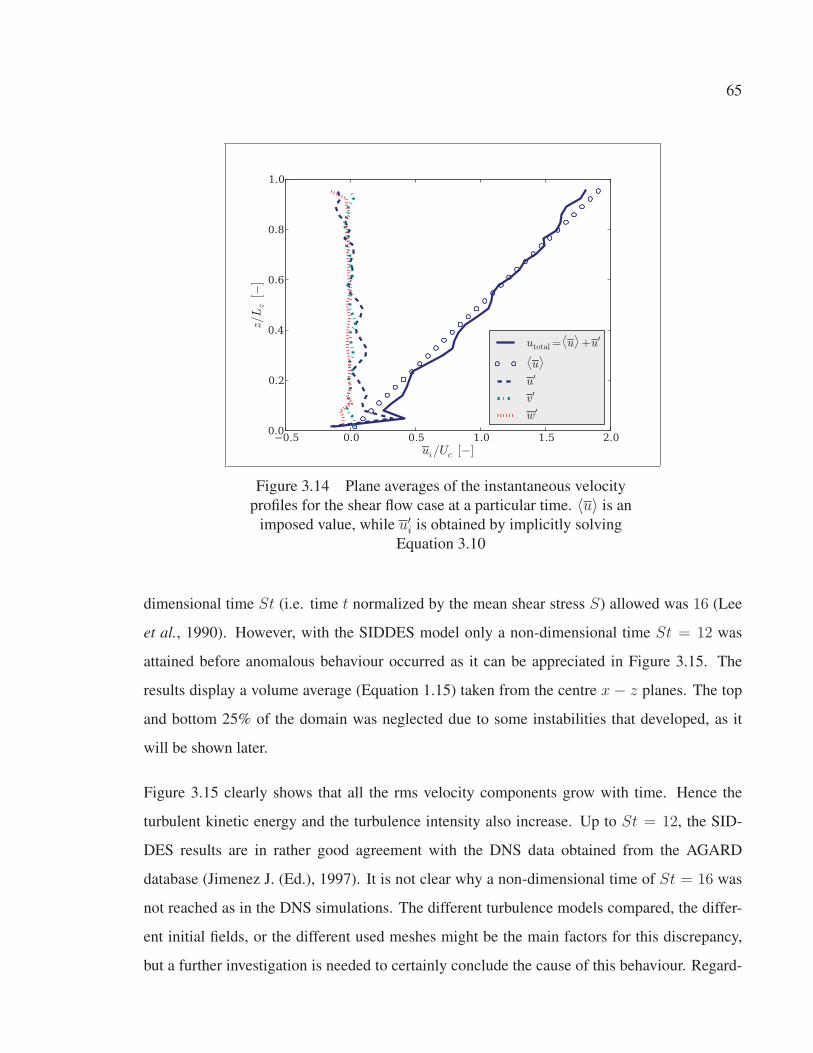
65

0.0

0.2

0.4

0.6

0.8

1.0

z/Lz[−

]

0.5 0.0 0.5 1.0 1.5 2.0

ui/Uc [−]

utotal =⟨u⟩+u′

⟨u⟩

u′

v′

w′

Figure 3.14 Plane averages of the instantaneous velocity

profiles for the shear flow case at a particular time. 〈u〉 is an

imposed value, while u′i is obtained by implicitly solving

Equation 3.10

dimensional time St (i.e. time t normalized by the mean shear stress S) allowed was 16 (Lee

et al., 1990). However, with the SIDDES model only a non-dimensional time St = 12 was

attained before anomalous behaviour occurred as it can be appreciated in Figure 3.15. The

results display a volume average (Equation 1.15) taken from the centre x − z planes. The top

and bottom 25% of the domain was neglected due to some instabilities that developed, as it

will be shown later.

Figure 3.15 clearly shows that all the rms velocity components grow with time. Hence the

turbulent kinetic energy and the turbulence intensity also increase. Up to St = 12, the SID-

DES results are in rather good agreement with the DNS data obtained from the AGARD

database (Jimenez J. (Ed.), 1997). It is not clear why a non-dimensional time of St = 16 was

not reached as in the DNS simulations. The different turbulence models compared, the differ-

ent initial fields, or the different used meshes might be the main factors for this discrepancy,

but a further investigation is needed to certainly conclude the cause of this behaviour. Regard-

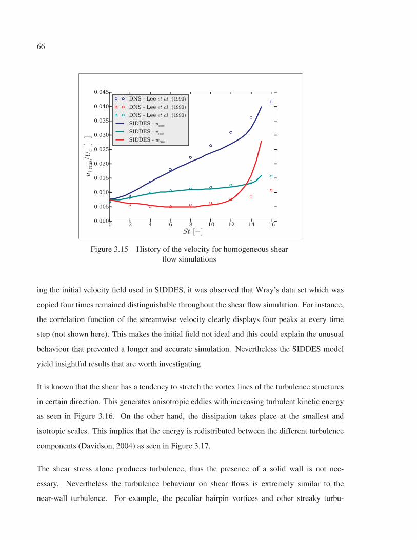
66

0 2 4 6 8 10 12 14 16

St [−]

0.000

0.005

0.010

0.015

0.020

0.025

0.030

0.035

0.040

0.045uirm

s/U

c[−

]

DNS - Lee et al. (1990)



SIDDES - urms

SIDDES - vrms

SIDDES - wrms

Figure 3.15 History of the velocity for homogeneous shear

flow simulations

ing the initial velocity field used in SIDDES, it was observed that Wray’s data set which was

copied four times remained distinguishable throughout the shear flow simulation. For instance,

the correlation function of the streamwise velocity clearly displays four peaks at every time

step (not shown here). This makes the initial field not ideal and this could explain the unusual

behaviour that prevented a longer and accurate simulation. Nevertheless the SIDDES model

yield insightful results that are worth investigating.

It is known that the shear has a tendency to stretch the vortex lines of the turbulence structures

in certain direction. This generates anisotropic eddies with increasing turbulent kinetic energy

as seen in Figure 3.16. On the other hand, the dissipation takes place at the smallest and

isotropic scales. This implies that the energy is redistributed between the different turbulence

components (Davidson, 2004) as seen in Figure 3.17.

The shear stress alone produces turbulence, thus the presence of a solid wall is not nec-

essary. Nevertheless the turbulence behaviour on shear flows is extremely similar to the

near-wall turbulence. For example, the peculiar hairpin vortices and other streaky turbu-

67

(a) St = 0.0

(b) St = 0.5

Figure 3.16 Streamwise velocity contours on the

x− y plane. Units: [m/s].

lence structures found on wall-bounded flows are also characteristic features of turbulent shear

flows (Rogers and Moin, 1987; Lee et al., 1990). This phenomena was also observed on the

SIDDES results. Figure 3.18 shows snapshots of the vorticity of the fluctuating velocity field

(ω = ∇× u′). The isotropic initial field is seen at St = 0, but at later times the elongated tur-

bulence structures are clearly distinguished. Surely in real flows, the shear is mostly generated

by a solid surface (i.e. no-slip condition) (Sagaut and Cambon, 2008). However certain cases

like the velocity deficit on a turbine wake could be characterized as a unbounded shear flow.

Finally, the production to dissipation ratio in this highly-sheared turbulent flow is displayed in

Figure 3.19. The SIDDES simulation results are consistent with the DNS; furthermore P/ε > 1

as the experimental results from Tavoularis and Karnik (1989) concluded. Once again this plot

shows that the SIDDES are presents a higher turbulent kinetic energy production than it can be

locally compensated by dissipation.

68

0 2 4 6 8 10 12 14 16

St [−]

0.0

0.2

0.4

0.6

0.8

1.0

ui2 rms/(2k)[−

]DNS - Lee et al. (1990)




SIDDES - urms/(2k)

SIDDES - vrms/(2k)

SIDDES - wrms/(2k)

SIDDES - −uw/(2k)

Figure 3.17 Energy components evolution in

homogeneous shear turbulence

Peculiarly uniformed shear flow simulations prove to be quite unpredictable and hard to re-

produce with other mesh refinement or other flow parameters (i.e. different CFL). It is

not clear why this happens, but other authors have also experience similar unstable simu-

lations (Sukheswalla et al., 2013). Nevertheless the achieved hybrid and DNS results are

consistent and in agreement with other experimental findings. This indicates that the hybrid

model was able to reproduce the interaction between turbulence structures and mean shear cor-

rectly. Despite the good results, one must be aware that all eddy viscosity models, including

the k − ω SST-SIDDES, only evaluate the turbulence locally without taking the neighbouring

cells or the time history into account. This assumption can lead to erroneous results in cases

where the flow is subjected to sudden changes of shear whether in space or in time (Davidson,

2004). Similarly, eddy viscosity models cannot accurately account for the dynamics of severe

anisotropy structures produced by strong shear or a strong rotation (Pope, 1975). For the hybrid

model in the LES region, the advantage is that the eddy viscosity assumptions concern only the

small subgrid scales (Bechmann, 2006).

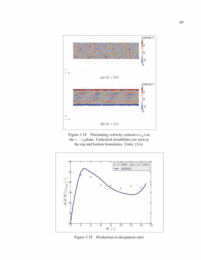
69

(a) St = 0.0

(b) St = 0.5

Figure 3.18 Fluctuating vorticity contours (ωy) on

the x− y plane. Undesired instabilities are seen at

the top and bottom boundaries. Units: [1/s].

0 2 4 6 8 10 12 14 16

St [−]

0

1

2

3

4

5

6

−S⟨ u

′w′⟩/ε t

otal[−

]


SIDDES

Figure 3.19 Production to dissipation ratio

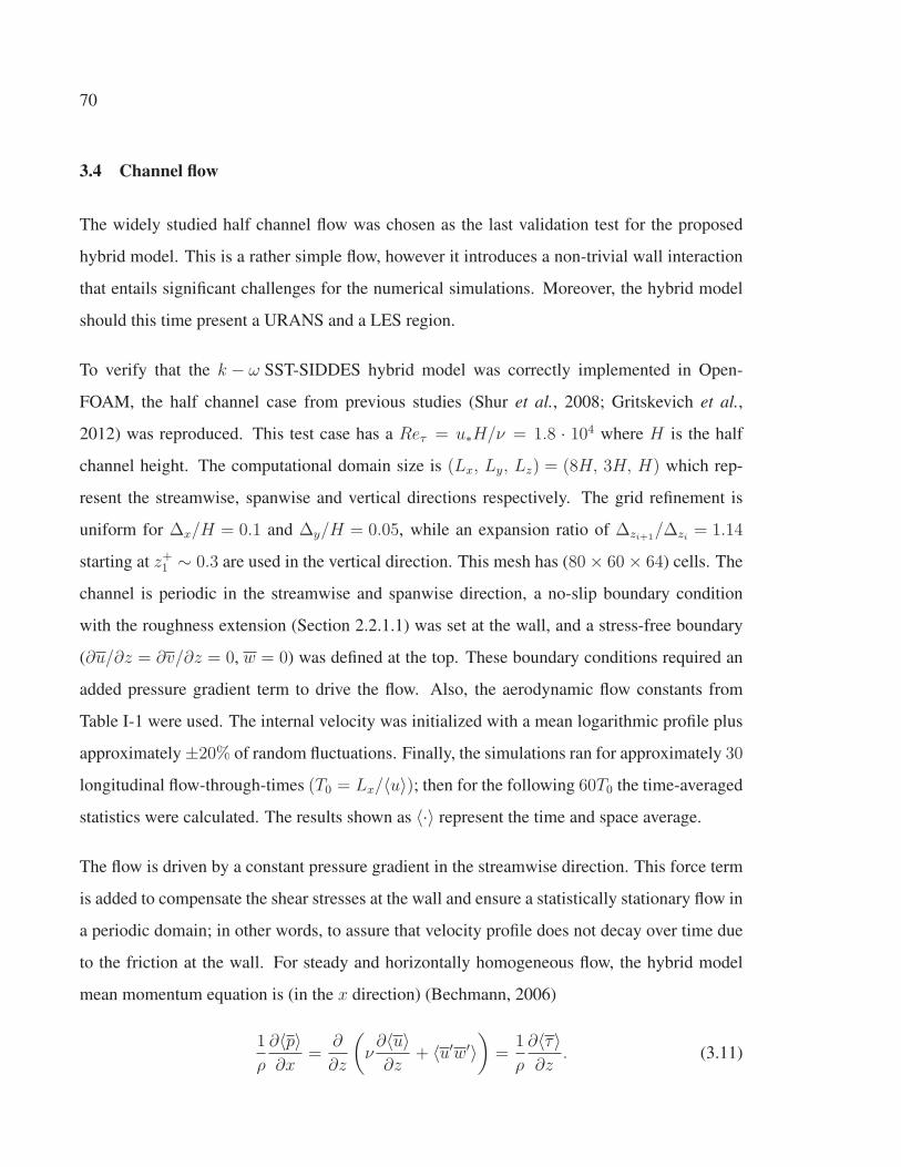
70

3.4 Channel flow

The widely studied half channel flow was chosen as the last validation test for the proposed

hybrid model. This is a rather simple flow, however it introduces a non-trivial wall interaction

that entails significant challenges for the numerical simulations. Moreover, the hybrid model

should this time present a URANS and a LES region.

To verify that the k − ω SST-SIDDES hybrid model was correctly implemented in Open-

FOAM, the half channel case from previous studies (Shur et al., 2008; Gritskevich et al.,

2012) was reproduced. This test case has a Reτ = u∗H/ν = 1.8 · 104 where H is the half

channel height. The computational domain size is (Lx, Ly, Lz) = (8H, 3H, H) which rep-

resent the streamwise, spanwise and vertical directions respectively. The grid refinement is

uniform for Δx/H = 0.1 and Δy/H = 0.05, while an expansion ratio of Δzi+1/Δzi = 1.14

starting at z+1 ∼ 0.3 are used in the vertical direction. This mesh has (80× 60× 64) cells. The

channel is periodic in the streamwise and spanwise direction, a no-slip boundary condition

with the roughness extension (Section 2.2.1.1) was set at the wall, and a stress-free boundary

(∂u/∂z = ∂v/∂z = 0, w = 0) was defined at the top. These boundary conditions required an

added pressure gradient term to drive the flow. Also, the aerodynamic flow constants from

Table I-1 were used. The internal velocity was initialized with a mean logarithmic profile plus

approximately ±20% of random fluctuations. Finally, the simulations ran for approximately 30

longitudinal flow-through-times (T0 = Lx/〈u〉); then for the following 60T0 the time-averaged

statistics were calculated. The results shown as 〈·〉 represent the time and space average.

The flow is driven by a constant pressure gradient in the streamwise direction. This force term

is added to compensate the shear stresses at the wall and ensure a statistically stationary flow in

a periodic domain; in other words, to assure that velocity profile does not decay over time due

to the friction at the wall. For steady and horizontally homogeneous flow, the hybrid model

mean momentum equation is (in the x direction) (Bechmann, 2006)

1

ρ

∂〈p〉∂x

=∂

∂z

(ν∂〈u〉∂z

+ 〈u′w′〉)

=1

ρ

∂〈τ〉∂z

. (3.11)

71

By integrating this equation over the whole domain height, and assuming that τ = 0 at the top

(z = H), it is found that

〈τ〉 = H∂〈p〉∂x

( z

H− 1

). (3.12)

At z = 0, the shear stresses are τw = −ρu2∗, hence

〈τw〉 = −H∂〈p〉∂x

= −ρu2∗. (3.13)

Thus the force term imposed in the Equation 2.12 corresponds to

Fx =∂〈p〉∂x

=ρu2

∗H

. (3.14)

It is sometimes referred as the large scale pressure gradient.

The large scale pressure gradient was implemented in OpenFOAM as a steady value based on

an imposed u∗ (Refer to Appendix III.3 for code details). On the contrary, the channelFoam

solver and a possible option on the SOWFA2 solvers use an imposed value of velocity at the top

of the domain to calculate and correct an unsteady large scale pressure gradient at each time

step to ensure the correct velocity at the top boundary. However an unsteady pressure gradient

might cover up the LLM that could occur when using the k − ω SST-SIDDES.

OpenFOAM has a second-order spatial discretization (See Section 2.1.3), therefore the

schemes used in the model implementation are all second-order. On the contrary the orig-

inal reference case uses fourth-order central schemes. For this reason, it is expected that the

shear stresses from the OpenFOAM implementation will not be as precise as the reference case

(for the same mesh refinement). This is shown in Figure 3.20. Additionally it was observed

that when a URANS region is present, these hybrid simulations become more unstable and tend

to diverge more easily if only central schemes are used to discretized the divergence terms of

2Wind energy software toolbox developed by Matt Churchfield and Sang Lee of the National Renewable

Energy Laboratory. It is based on OpenFOAM. More details can be found at NWTC Information Portal (SOWFA).

https://nwtc.nrel.gov/SOWFA.

72

the equations. For this reason blended discretization schemes are chosen; they are called local-

Blending in the OpenFOAM code. A blendingFactor is defined based on the local and instan-

taneous URANS and LES regions in the domain. For cells located in pure URANS regions, the

blendingFactor is defined as 0 and the second-order upwind (linearUpwind) scheme is chosen;

while for cell in pure LES zones, the blendingFactor equals to 1.0 and the second-order central

(linear) scheme is used. Consequently a scheme with some upwind and central components is

used for the blended URANS/LES regions (For a detailed explanation of the implementation

and use in OpenFOAM see Appendix III.5 and III.6). To be consistent, second-order backward

scheme is always employed for the temporal discretization.

1.0 0.8 0.6 0.4 0.2 0.0⟨τxz

⟩/ρu 2

∗[−]

0.0

0.2

0.4

0.6

0.8

1.0

z/H

[−]

τresolved = −ρu′w′

τmodelled = 2νtSxz

τviscous = ν u/ z

τresolved - Shur et al. (2008)

τmodelled - Shur et al. (2008)

(a) CFL=0.2

1.0 0.8 0.6 0.4 0.2 0.0⟨τxz

⟩/ρu 2

∗[−]

0.0

0.2

0.4

0.6

0.8

1.0

z/H

[−]



τviscous = ν u/ z



(b) CFL=0.7

Figure 3.20 Averaged shear stresses for a smooth half channel flow using central

discretization schemes for the divergence term on the transport and model equations.

These SIDDES results are compared against the reference article data (Shur et al.,2008).

Figure 3.21 shows the viscosity ratio 〈νt〉/ν for half channel simulations using different dis-

cretization schemes for the convective terms. The turbulent viscosity increases in the URANS

regions, then around z+ ≈ 103 the hybrid switches to LES and the eddy viscosity starts di-

minishing. The discretization schemes do not have an impact on the height at which the

URANS zones transition to LES. However, the results that agree better with the benchmark

case use pure central schemes to discretized the convective terms in the momentum equation

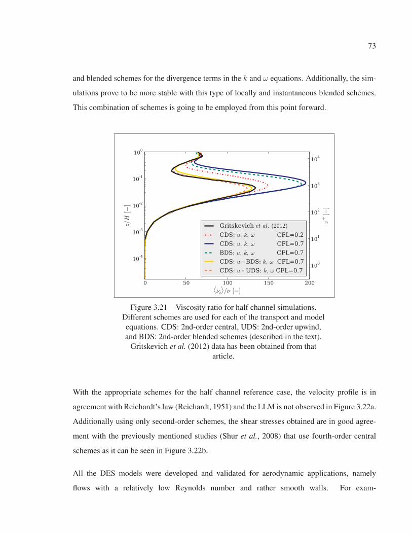
73

and blended schemes for the divergence terms in the k and ω equations. Additionally, the sim-

ulations prove to be more stable with this type of locally and instantaneous blended schemes.

This combination of schemes is going to be employed from this point forward.

100

101

102

103

104

z+[−

]

10-4

10-3

10-2

10-1

100

z/H

[−]

0 50 100 150 200⟨νt⟩/ν [−]

Gritskevich et al. (2012)

CDS: u, k, ω CFL=0.2

CDS: u, k, ω CFL=0.7

BDS: u, k, ω CFL=0.7

CDS: u - BDS: k, ω CFL=0.7

CDS: u - UDS: k, ω CFL=0.7

Figure 3.21 Viscosity ratio for half channel simulations.

Different schemes are used for each of the transport and model

equations. CDS: 2nd-order central, UDS: 2nd-order upwind,

and BDS: 2nd-order blended schemes (described in the text).

Gritskevich et al. (2012) data has been obtained from that

article.

With the appropriate schemes for the half channel reference case, the velocity profile is in

agreement with Reichardt’s law (Reichardt, 1951) and the LLM is not observed in Figure 3.22a.

Additionally using only second-order schemes, the shear stresses obtained are in good agree-

ment with the previously mentioned studies (Shur et al., 2008) that use fourth-order central

schemes as it can be seen in Figure 3.22b.

All the DES models were developed and validated for aerodynamic applications, namely

flows with a relatively low Reynolds number and rather smooth walls. For exam-

74

10-4

10-3

10-2

10-1

100

z/H [−]

0

5

10

15

20

25

30

⟨ u⟩ /u∗[−

]

100

101

102

103

104

z+ [−]

k−ω SST-SIDDES

Reichardt's law

(a) Averaged velocity profiles

1.0 0.8 0.6 0.4 0.2 0.0⟨τxz

⟩/ρu 2

∗[−]

0.0

0.2

0.4

0.6

0.8

1.0

z/H

[−]



τviscous = ν u/ z



(b) Averaged shear stresses

Figure 3.22 Half channel flow at Reτ = 1.8 · 104 using blended schemes for the

divergence terms in the k and ω equations and imposing a maximum CFL=0.7. Shur

et al. (2008) data has been digitized.

ple, the IDDES model has been validated for smooth channel flow simulation up to

Reτ = u∗H/ν = 1.8 · 104, where u∗ is the friction velocity and H represents the half

channel height (Shur et al., 2008); the same for SIDDES (Gritskevich et al., 2012).

On the contrary, the ABL simulations required by the wind energy industry involve

extremely high Reynolds numbers (Reτ ∼ 107 − 109) and exceedingly high roughness

(z0 ∼ 0.00001− 0.5 m depending on the terrain (Manwell et al., 2002)). Therefore, the be-

haviour of the DES hybrid models still need to be validated for the ABL specifications.

To this end, SIDDES half channel flow simulations were performed for a series of higher

Reynolds numbers3 ReDh= UavDh/ν and then for rough walls covering all across the avail-

able data in the Moody chart (White, 1991). Dh = 4H represents the hydraulic diame-

ter of a channel with a height of 2H and periodic lateral boundaries, and Uav is the av-

erage velocity. The aim is to verify if the LLM correction is still valid for other parame-

ters not tested by (Gritskevich et al., 2012). As a reference, Shur et al. (2008) case has a

ReDh= 1.9 · 106 and a relative pipe roughness ks/Dh = 0, while a typical ABL simulation

could reach ReDh= 1 · 108 and relative pipe roughness of ks/Dh = 30z0/4H = 3 · 10−3 for a

3A Reτ ∼ 107 corresponds to ReDh∼ 108 − 109

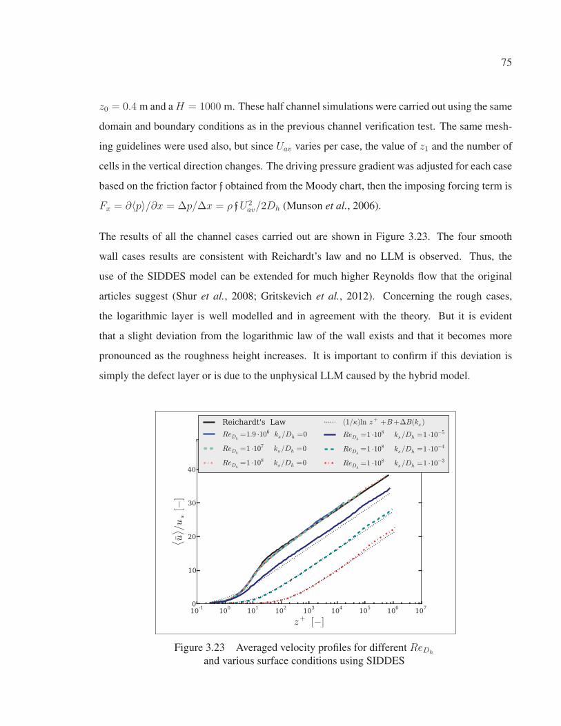
75

z0 = 0.4 m and a H = 1000 m. These half channel simulations were carried out using the same

domain and boundary conditions as in the previous channel verification test. The same mesh-

ing guidelines were used also, but since Uav varies per case, the value of z1 and the number of

cells in the vertical direction changes. The driving pressure gradient was adjusted for each case

based on the friction factor f obtained from the Moody chart, then the imposing forcing term is

Fx = ∂〈p〉/∂x = Δp/Δx = ρ fU2av/2Dh (Munson et al., 2006).

The results of all the channel cases carried out are shown in Figure 3.23. The four smooth

wall cases results are consistent with Reichardt’s law and no LLM is observed. Thus, the

use of the SIDDES model can be extended for much higher Reynolds flow that the original

articles suggest (Shur et al., 2008; Gritskevich et al., 2012). Concerning the rough cases,

the logarithmic layer is well modelled and in agreement with the theory. But it is evident

that a slight deviation from the logarithmic law of the wall exists and that it becomes more

pronounced as the roughness height increases. It is important to confirm if this deviation is

simply the defect layer or is due to the unphysical LLM caused by the hybrid model.

10-1

100

101

102

103

104

105

106

107

z+ [−]

0

10

20

30

40

⟨ u⟩ /u∗[−

]

Reichardt's Law

ReDh=1.9 ·106 ks /Dh =0

ReDh=1 ·107 ks /Dh =0

ReDh=1 ·108 ks /Dh =0

(1/κ)ln z+ +B+ΔB(ks )

ReDh=1 ·108 ks /Dh =1 ·10−5

ReDh=1 ·108 ks /Dh =1 ·10−4

ReDh=1 ·108 ks /Dh =1 ·10−3

Figure 3.23 Averaged velocity profiles for different ReDh

and various surface conditions using SIDDES

76

The defect layer behaviour

uDefect =〈u0〉 − 〈u〉

u∗(3.15)

has been studied in the past for smooth and rough turbulent pipe flow. Here 〈u0〉 is the mean

velocity at the top of the half channel. Coles’ law of the wake as well as the velocity-defect

distribution obtained from Laufer’s experimental data describe this deviation from the logarith-

mic layer (Hinze, 1975). It is known, that the logarithmic layer exist up to a height of 0.15H

for boundary layers and pipe flows (Hinze, 1975), but the behaviour above that height has not

been thoroughly studied especially on channel flow. The velocity-defect for the channel cases

is shown in Figure 3.24. Regardless of the type of surface, all the velocity-defect curves col-

lapse, confirming that the wall roughness does not have an impact on the defect layer (White,

1991). However, the velocity profiles start deviating from the log-law slightly below 0.1H ,

and also, there is a disagreement between Laufer’s measured velocity distribution and the sim-

ulations results. For the lack of more exhaustive studied on the defect law, it is a hard task

to distinguishing if the observed deviation is related to the hybrid model or to the defect layer

behaviour. However, this findings may suggest that there is still a slight LLM for all the chan-

nel flow simulations done using the k − ω SST-SIDDES model. Another possibility to explain

these results might be an speed up effect caused by the domain size. This effect was observed

for the pressure driven atmospheric boundary simulations carried out in Section 4.2.

3.5 Summary

A step by step validation of the k − ω SST-SIDDES model has been carried out on canonical

flows. The investigation of this mostly theoretical cases provide the opportunity to examine

certain turbulence properties in an isolated manner. In other words the development of isotropic

or anisotropic eddies, the effect that rotation or shear forces have on the overall flow, and finally

the impact of a solid wall were analyzed independently. This particular understanding is highly

detailed and theoretical, but it will certainly be advantageous when more complex flows are

modelled.

77

10-2

10-1

100

ζ=z/H [−]

0

2

4

6

8

10

12

14

uDefect=

( ⟨ u0

⟩ −⟨ u⟩) /

u∗[−

]

UDefect =−2.44 ln ζ+0.8

ReDh=1.9 ·106 ks /Dh =0

ReDh=1 ·107 ks /Dh =0

ReDh=1 ·108 ks /Dh =0

UDefect =7.2 (1−ζ)2

ReDh=1 ·108 ks /Dh =1 ·10−5

ReDh=1 ·108 ks /Dh =1 ·10−4

ReDh=1 ·108 ks /Dh =1 ·10−3

Figure 3.24 Averaged velocity-defect profiles for different ReDhand

surface conditions using the SIDDES turbulence model compared

against Laufer’s measured velocity-defect distributions.

Concerning the hybrid model, it was demonstrated that it reproduces all tested the canonical

flows correctly. But most importantly, this validation helped determine the proper discretization

schemes. These chosen schemes allow the proper modelling of the turbulent flow and at the

same time ensure the stability of the simulations. Now, the hybrid model can be used with

confidence for flat terrain simulations.

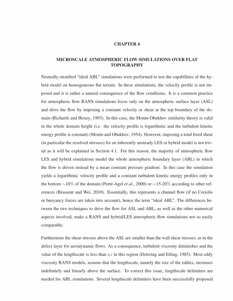
CHAPTER 4

MICROSCALE ATMOSPHERIC FLOW SIMULATIONS OVER FLATTOPOGRAPHY

Neutrally-stratified “ideal ABL” simulations were performed to test the capabilities of the hy-

brid model on homogeneous flat terrain. In these simulations, the velocity profile is not im-

posed and it is rather a natural consequence of the flow conditions. It is a common practice

for atmospheric flow RANS simulations focus only on the atmospheric surface layer (ASL)

and drive the flow by imposing a constant velocity or shear at the top boundary of the do-

main (Richards and Hoxey, 1993). In this case, the Monin-Obukhov similarity theory is valid

in the whole domain height (i.e. the velocity profile is logarithmic and the turbulent kinetic

energy profile is constant) (Monin and Obukhov, 1954). However, imposing a total fixed shear

(in particular the resolved stresses) for an inherently unsteady LES or hybrid model is not triv-

ial as it will be explained in Section 4.1. For this reason, the majority of atmospheric flow

LES and hybrid simulations model the whole atmospheric boundary layer (ABL) in which

the flow is driven instead by a mean constant pressure gradient. In this case the simulation

yields a logarithmic velocity profile and a constant turbulent kinetic energy profiles only in

the bottom ∼10% of the domain (Porté-Agel et al., 2000) or ∼15-20% according to other ref-

erences (Brasseur and Wei, 2010). Essentially, this represents a channel flow (if no Coriolis

or buoyancy forces are taken into account), hence the term “ideal ABL”. The differences be-

tween the two techniques to drive the flow for ASL and ABL, as well as the other numerical

aspects involved, make a RANS and hybrid/LES atmospheric flow simulations not so easily

comparable.

Furthermore the shear stresses above the ASL are smaller than the wall shear stresses, as in the

defect layer for aerodynamic flows. As a consequence, turbulent viscosity diminishes and the

value of the lengthscale is less than κz in this region (Detering and Etling, 1985). Most eddy

viscosity RANS models, assume that the lengthscale, namely the size of the eddies, increases

indefinitely and linearly above the surface. To correct this issue, lengthscale delimiters are

needed for ABL simulations. Several lengthscale delimiters have been successfully proposed

80

mostly for k − ε models (Sumner and Masson, 2012) but not for k − ω SST. This problem is

not present in the hybrid models since the RANS region does not generally extend above the

surface layer.

Considering these issues, several simulations of the atmospheric flow in flat and homoge-

neously rough terrain will be performed in this chapter. First the neutral atmospheric surface

layer will be studied. Then the neutrally stratified boundary layer will be characterized as a

pressured-driven flow. Then, the effects of the Coriolis force will also be analyzed for the ideal

ABL. To conclude this validation process, a field measurement campaign over a natural flat

terrain will be studied. The current flat terrain study attempts to anticipate and eliminate the

forthcoming problems that might be encounter in other types of terrain.

4.1 Atmospheric surface layer 1

The atmospheric surface layer represents approximately 10% of the atmospheric boundary

layer. It is characterized by constant shear stresses on the vertical direction and a logarithmic

velocity profile. To model this region three turbulence models are investigated to model the

ASL: the RANS k − ω SST, and the hybrids k − ω SST-DES and k − ω SST-SIDDES.

For these simulations, a domain of size of (Lx, Ly, Lz) = (3H, 3H, H) where H = 1000 m

is used. The bottom boundary is placed at the roughness height of z0 = 0.1 m as illustrated in

Figure 1.1. A z+1 ∼ 1.0 is implemented instead of 0.3 as required by the roughness extension.

This compromise was necessary to alleviate the constrains on blockMesh, the OpenFOAM

mesh generator, which was not giving accurate results (i.e. the lowest row of cells was too small

and could not achieve a constant height possibly due to round off errors). These tests brought

forward the fact that the model requires a good quality mesh generator capable of properly

defining the height of the fist node and handling high aspect ratio near-wall cells. From the

wall surface, an expansion ratio of Δzi+1/Δzi ∼ 1.15 is set up until the size of the cell Δz

1Preliminary results of this section were published as the conference article: Bautista. M. C., Dufresne L.,

and Masson C. "Hybrid turbulence models for atmospheric flow. A proper comparison with RANS models”. In

The Second Symposium on OpenFOAM R© in Wind Energy. (Boulder, CO., USA) May 19-21, 2014.

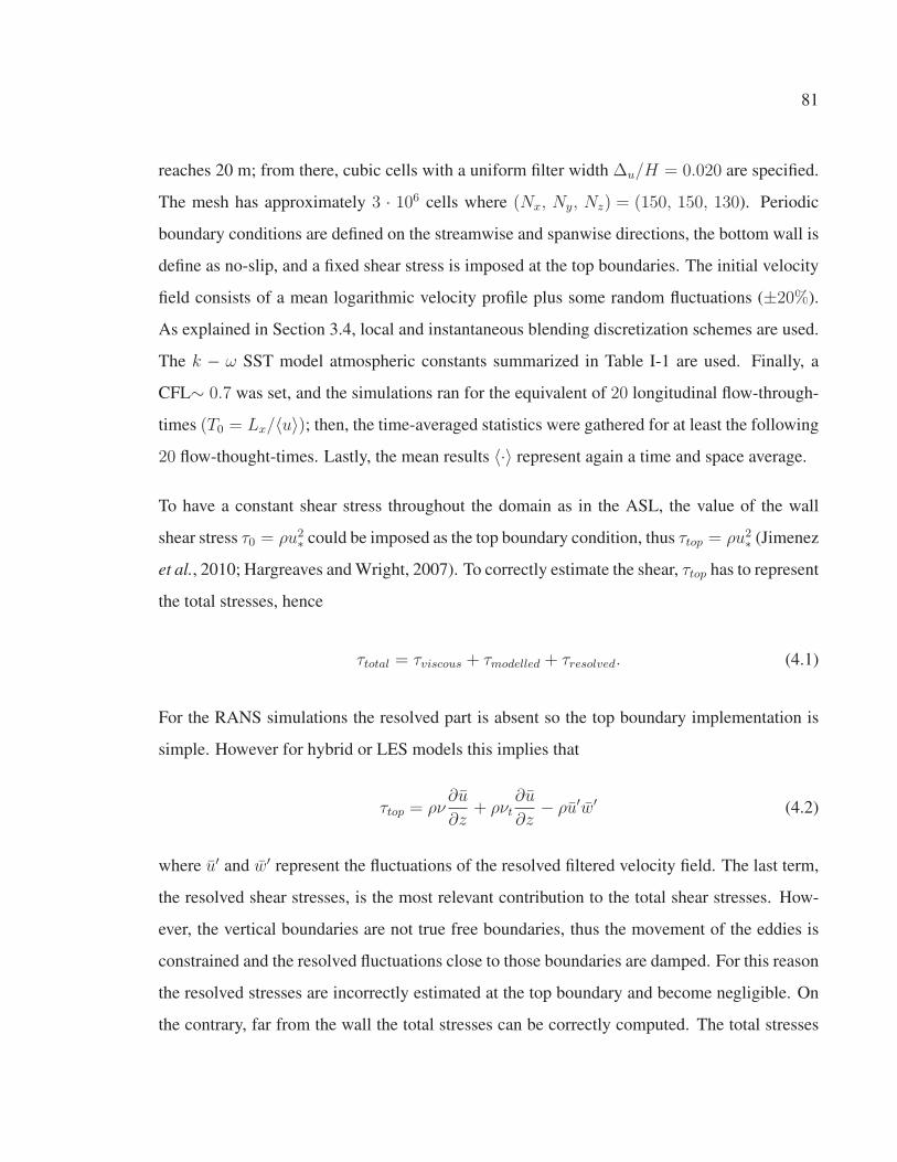
81

reaches 20 m; from there, cubic cells with a uniform filter width Δu/H = 0.020 are specified.

The mesh has approximately 3 · 106 cells where (Nx, Ny, Nz) = (150, 150, 130). Periodic

boundary conditions are defined on the streamwise and spanwise directions, the bottom wall is

define as no-slip, and a fixed shear stress is imposed at the top boundaries. The initial velocity

field consists of a mean logarithmic velocity profile plus some random fluctuations (±20%).

As explained in Section 3.4, local and instantaneous blending discretization schemes are used.

The k − ω SST model atmospheric constants summarized in Table I-1 are used. Finally, a

CFL∼ 0.7 was set, and the simulations ran for the equivalent of 20 longitudinal flow-through-

times (T0 = Lx/〈u〉); then, the time-averaged statistics were gathered for at least the following

20 flow-thought-times. Lastly, the mean results 〈·〉 represent again a time and space average.

To have a constant shear stress throughout the domain as in the ASL, the value of the wall

shear stress τ0 = ρu2∗ could be imposed as the top boundary condition, thus τtop = ρu2

∗ (Jimenez

et al., 2010; Hargreaves and Wright, 2007). To correctly estimate the shear, τtop has to represent

the total stresses, hence

τtotal = τviscous + τmodelled + τresolved. (4.1)

For the RANS simulations the resolved part is absent so the top boundary implementation is

simple. However for hybrid or LES models this implies that

τtop = ρν∂u

∂z+ ρνt

∂u

∂z− ρu′w′ (4.2)

where u′ and w′ represent the fluctuations of the resolved filtered velocity field. The last term,

the resolved shear stresses, is the most relevant contribution to the total shear stresses. How-

ever, the vertical boundaries are not true free boundaries, thus the movement of the eddies is

constrained and the resolved fluctuations close to those boundaries are damped. For this reason

the resolved stresses are incorrectly estimated at the top boundary and become negligible. On

the contrary, far from the wall the total stresses can be correctly computed. The total stresses

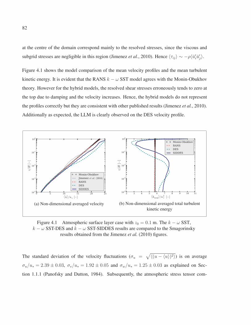
82

at the centre of the domain correspond mainly to the resolved stresses, since the viscous and

subgrid stresses are negligible in this region (Jimenez et al., 2010). Hence 〈τij〉 ∼ −ρ〈u′iu

′j〉.

Figure 4.1 shows the model comparison of the mean velocity profiles and the mean turbulent

kinetic energy. It is evident that the RANS k − ω SST model agrees with the Monin-Obukhov

theory. However for the hybrid models, the resolved shear stresses erroneously tends to zero at

the top due to damping and the velocity increases. Hence, the hybrid models do not represent

the profiles correctly but they are consistent with other published results (Jimenez et al., 2010).

Additionally as expected, the LLM is clearly observed on the DES velocity profile.

0 5 10 15 20 25⟨u⟩/u

∗[−]

10-4

10-3

10-2

10-1

100

z/H

[−]

Monin-Obukhov

Jimenez et al. (2010)

RANS

DES

SIDDES

(a) Non-dimensional averaged velocity

2 3 4 5 6 7 8 9 10 11⟨ktotal

⟩/u 2

∗[−]

10-4

10-3

10-2

10-1

100

z/H

[−]

Monin-Obukhov

RANS

DES

SIDDES

(b) Non-dimensional averaged total turbulent

kinetic energy

Figure 4.1 Atmospheric surface layer case with z0 = 0.1 m. The k − ω SST,

k − ω SST-DES and k − ω SST-SIDDES results are compared to the Smagorinsky

results obtained from the Jimenez et al. (2010) figures.

The standard deviation of the velocity fluctuations (σu =√〈(u− 〈u〉)2〉) is on average

σu/u∗ = 2.39± 0.03, σv/u∗ = 1.92± 0.05 and σw/u∗ = 1.25± 0.03 as explained on Sec-

tion 1.1.1 (Panofsky and Dutton, 1984). Subsequently, the atmospheric stress tensor com-

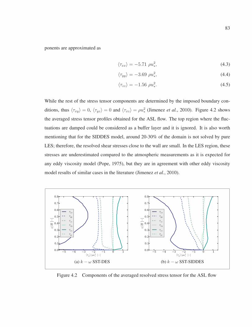
83

ponents are approximated as

〈τxx〉 = −5.71 ρu2∗, (4.3)

〈τyy〉 = −3.69 ρu2∗, (4.4)

〈τzz〉 = −1.56 ρu2∗. (4.5)

While the rest of the stress tensor components are determined by the imposed boundary con-

ditions, thus 〈τxy〉 = 0, 〈τyz〉 = 0 and 〈τxz〉 = ρu2∗ (Jimenez et al., 2010). Figure 4.2 shows

the averaged stress tensor profiles obtained for the ASL flow. The top region where the fluc-

tuations are damped could be considered as a buffer layer and it is ignored. It is also worth

mentioning that for the SIDDES model, around 20-30% of the domain is not solved by pure

LES; therefore, the resolved shear stresses close to the wall are small. In the LES region, these

stresses are underestimated compared to the atmospheric measurements as it is expected for

any eddy viscosity model (Pope, 1975), but they are in agreement with other eddy viscosity

model results of similar cases in the literature (Jimenez et al., 2010).

5 4 3 2 1 0 1⟨τij

⟩/ρu 2

∗[−]

0.0

0.1

0.2

0.3

0.4

0.5

0.6

0.7

0.8

z/H

[−]

τxx

τyy

τzz

τxy

τxz

τyz

(a) k − ω SST-DES

5 4 3 2 1 0 1⟨τij

⟩/ρu 2

∗[−]

0.0

0.1

0.2

0.3

0.4

0.5

0.6

0.7

0.8

z/H

[−]

τxx

τyy

τzz

τxy

τxz

τyz

(b) k − ω SST-SIDDES

Figure 4.2 Components of the averaged resolved stress tensor for the ASL flow

84

Certain authors have taken advantage of the somewhat constant shear stresses obtained with

these boundary conditions to analyze turbine wakes (Jimenez et al., 2010). However, these

boundary conditions and the technique to drive the flow might not be suitable for atmospheric

flow simulations. Notably, a sophisticated unsteady boundary condition that does not constrain

the eddies movement would have to be implemented to correctly simulate the resolved stresses.

However, this is a complex task and not easy achievable. To bypass this problem, a pressure

driven flow is commonly enforced and the entire atmospheric boundary layer is simulated.

4.2 Idealized neutral atmospheric boundary layer

It was demonstrated that solving only the atmospheric surface layer using a hybrid model

does not yield ideal results due to the required boundary conditions. Therefore, the next step

is to simulate the whole yet simplified representation of the atmospheric boundary layer, as

the majority of LES and hybrid simulations do. In ABL simulations, the mechanisms that

drive the flow and the top boundary conditions are different from the previous ASL case.

Hence, ABL simulations should yield a logarithmic velocity profile and a constant turbulent

kinetic energy profiles only in the bottom ∼ 10− 20% of the domain (Porté-Agel et al., 2000;

Brasseur and Wei, 2010) if a well-behaved LES or hybrid model is used. However if an eddy

viscosity RANS model is employed, a lengthscale delimiter most be added to the original equa-

tions to account for the unphysical and unlimited increase of the calculated length scale (Sum-

ner and Masson, 2012). Only the length scale delimiter for k− ε models has been published in

the literature, and the extrapolation to the k − ω SST might not be as straightforward nor the

objective of this work. Therefore, the RANS ABL simulation will not be presented here.

4.2.1 Pressure driven atmospheric flow

A simplified neutral ABL simulation is carried out as a pressure driven flow, which is equiva-

lent to a channel flow. As in Section 3.4 a large pressure gradient source term is added to the

Navier-Stokes equations, thus Fx = ρu2∗/H in Equation 2.12. A stress-free boundary condition

is imposed at the top of the domain, while periodic boundaries are specified for the stream and

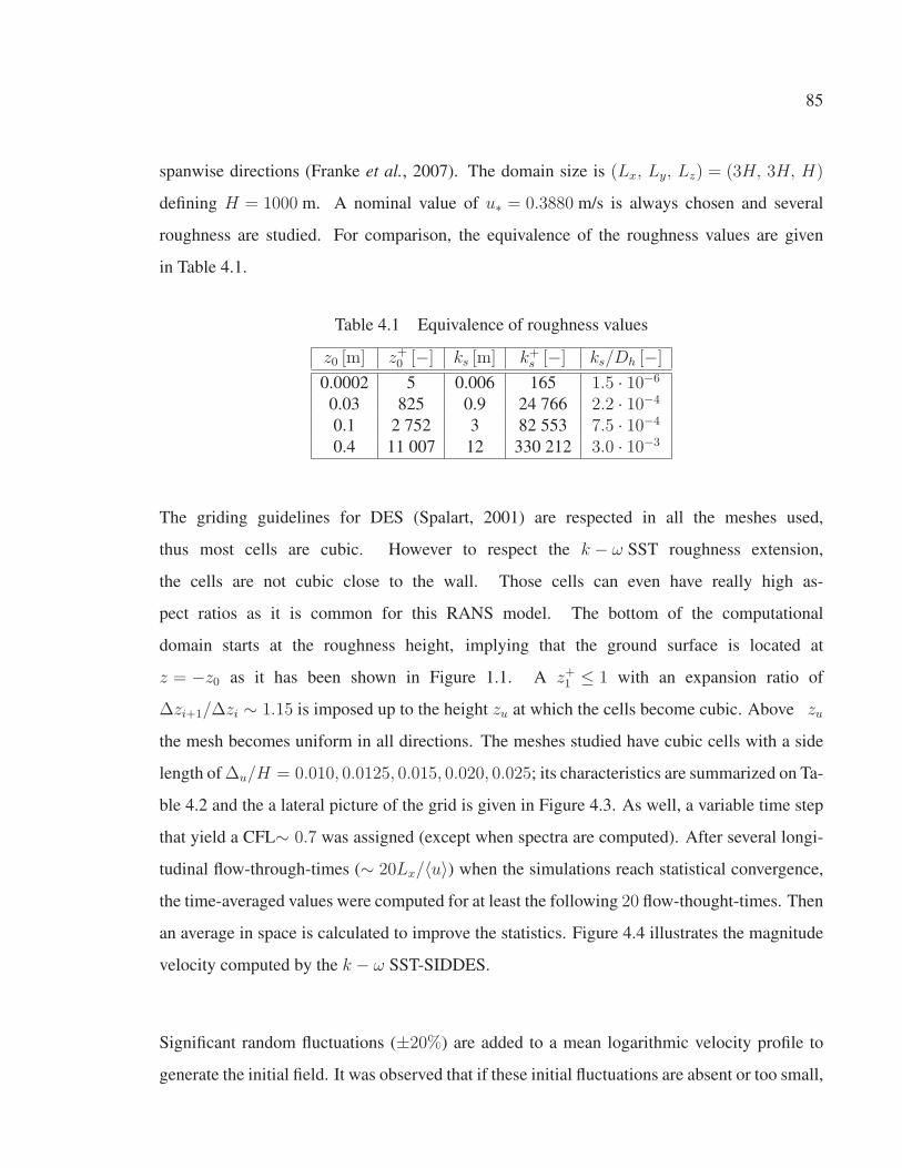
85

spanwise directions (Franke et al., 2007). The domain size is (Lx, Ly, Lz) = (3H, 3H, H)

defining H = 1000 m. A nominal value of u∗ = 0.3880 m/s is always chosen and several

roughness are studied. For comparison, the equivalence of the roughness values are given

in Table 4.1.

Table 4.1 Equivalence of roughness values

z0 [m] z+0 [−] ks [m] k+s [−] ks/Dh [−]

0.0002 5 0.006 165 1.5 · 10−6

0.03 825 0.9 24 766 2.2 · 10−4

0.1 2 752 3 82 553 7.5 · 10−4

0.4 11 007 12 330 212 3.0 · 10−3

The griding guidelines for DES (Spalart, 2001) are respected in all the meshes used,

thus most cells are cubic. However to respect the k − ω SST roughness extension,

the cells are not cubic close to the wall. Those cells can even have really high as-

pect ratios as it is common for this RANS model. The bottom of the computational

domain starts at the roughness height, implying that the ground surface is located at

z = −z0 as it has been shown in Figure 1.1. A z+1 ≤ 1 with an expansion ratio of

Δzi+1/Δzi ∼ 1.15 is imposed up to the height zu at which the cells become cubic. Above zu

the mesh becomes uniform in all directions. The meshes studied have cubic cells with a side

length of Δu/H = 0.010, 0.0125, 0.015, 0.020, 0.025; its characteristics are summarized on Ta-

ble 4.2 and the a lateral picture of the grid is given in Figure 4.3. As well, a variable time step

that yield a CFL∼ 0.7 was assigned (except when spectra are computed). After several longi-

tudinal flow-through-times (∼ 20Lx/〈u〉) when the simulations reach statistical convergence,

the time-averaged values were computed for at least the following 20 flow-thought-times. Then

an average in space is calculated to improve the statistics. Figure 4.4 illustrates the magnitude

velocity computed by the k − ω SST-SIDDES.

Significant random fluctuations (±20%) are added to a mean logarithmic velocity profile to

generate the initial field. It was observed that if these initial fluctuations are absent or too small,

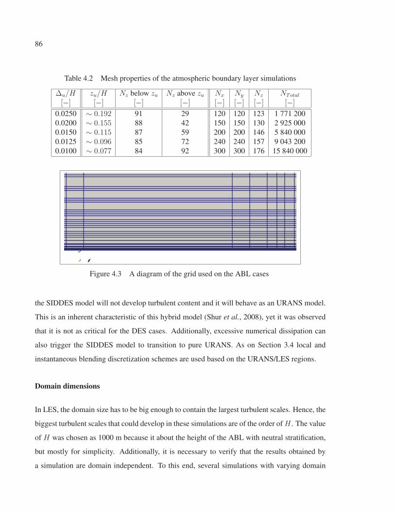
86

Table 4.2 Mesh properties of the atmospheric boundary layer simulations

Δu/H zu/H Nz below zu Nz above zu Nx Ny Nz NTotal

[−] [−] [−] [−] [−] [−] [−] [−]

0.0250 ∼ 0.192 91 29 120 120 123 1 771 200

0.0200 ∼ 0.155 88 42 150 150 130 2 925 000

0.0150 ∼ 0.115 87 59 200 200 146 5 840 000

0.0125 ∼ 0.096 85 72 240 240 157 9 043 200

0.0100 ∼ 0.077 84 92 300 300 176 15 840 000

Figure 4.3 A diagram of the grid used on the ABL cases

the SIDDES model will not develop turbulent content and it will behave as an URANS model.

This is an inherent characteristic of this hybrid model (Shur et al., 2008), yet it was observed

that it is not as critical for the DES cases. Additionally, excessive numerical dissipation can

also trigger the SIDDES model to transition to pure URANS. As on Section 3.4 local and

instantaneous blending discretization schemes are used based on the URANS/LES regions.

Domain dimensions

In LES, the domain size has to be big enough to contain the largest turbulent scales. Hence, the

biggest turbulent scales that could develop in these simulations are of the order of H . The value

of H was chosen as 1000 m because it about the height of the ABL with neutral stratification,

but mostly for simplicity. Additionally, it is necessary to verify that the results obtained by

a simulation are domain independent. To this end, several simulations with varying domain

87

Figure 4.4 Magnitude of the filtered instantaneous velocity field computed for

an ideal ABL simulation (Δu/H = 0.020 and a z0 = 0.4 m). The domain

dimensions and turbulent nature of the flow can be appreciated. Units: [m/s].

width were carried out while keeping the streamwise length as Lx = 3H and the height as

Lz = H . The results are compiled in Figure 4.5. When the domain width is smaller than 3H a

speed-up effect can be seen. This could be misinterpreted as being caused by the LLM. When

Ly = 3H , the simulations are not strictly domain independent. Nevertheless, the different in

the results is minimal and at the same time, the computational cost is kept low. Additionally,

other authors have used this domain size for ABL simulations (Brasseur and Wei, 2010).

SIDDES model constants calibration

The k−ω SST model constants for atmospheric flows given in Table I-1 are employed on these

cases. These constants have not been used in combination with DES and SIDDES, therefore

their overall effect on the results had to be studied. In has been shown for a similar DES

hybrid model, that the LES results do not depend on the RANS constant Cμ (equivalent to

β∗) (Bechmann and Sørensen, 2010), suggesting that the value of such constant is not relevant

in the LES region. Likewise for the k − ω SST-DES it was verified that the LES results are

not affected by the choice of RANS constants and the height at which URANS switches to

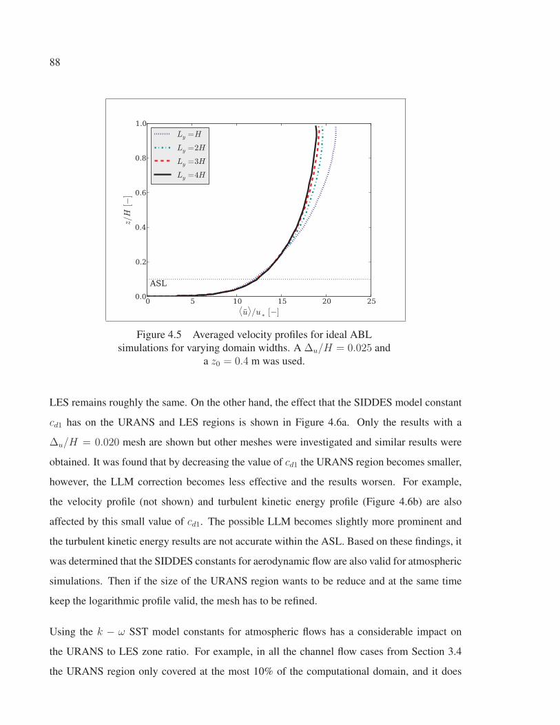
88

0.0

0.2

0.4

0.6

0.8

1.0z/H

[−]

0 5 10 15 20 25⟨u⟩/u

∗[−]

ASL

Ly =H

Ly =2H

Ly =3H

Ly =4H

Figure 4.5 Averaged velocity profiles for ideal ABL

simulations for varying domain widths. A Δu/H = 0.025 and

a z0 = 0.4 m was used.

LES remains roughly the same. On the other hand, the effect that the SIDDES model constant

cd1 has on the URANS and LES regions is shown in Figure 4.6a. Only the results with a

Δu/H = 0.020 mesh are shown but other meshes were investigated and similar results were

obtained. It was found that by decreasing the value of cd1 the URANS region becomes smaller,

however, the LLM correction becomes less effective and the results worsen. For example,

the velocity profile (not shown) and turbulent kinetic energy profile (Figure 4.6b) are also

affected by this small value of cd1. The possible LLM becomes slightly more prominent and

the turbulent kinetic energy results are not accurate within the ASL. Based on these findings, it

was determined that the SIDDES constants for aerodynamic flow are also valid for atmospheric

simulations. Then if the size of the URANS region wants to be reduce and at the same time

keep the logarithmic profile valid, the mesh has to be refined.

Using the k − ω SST model constants for atmospheric flows has a considerable impact on

the URANS to LES zone ratio. For example, in all the channel flow cases from Section 3.4

the URANS region only covered at the most 10% of the computational domain, and it does

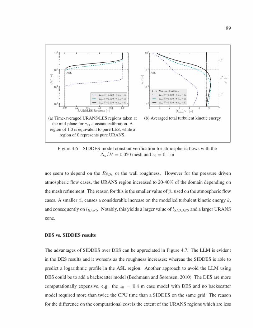
89

0.0 0.2 0.4 0.6 0.8 1.0

RANS/LES Regions [−]

10-3

10-2

10-1

100

z/H

[−] ASL

Δu /H=0.020 + cd1 =10

Δu /H=0.020 + cd1 =15

Δu /H=0.020 + cd1 =20

(a) Time-averaged URANS/LES regions taken at

the mid-plane for cd1 constant calibration. A

region of 1.0 is equivalent to pure LES, while a

region of 0 represents pure URANS.

105

106

107

z+

[−]

10-3

10-2

10-1

100

z/H

[−]

0 1 2 3 4 5 6 7⟨ktotal

⟩/u 2

∗[−]

ASL

Monin-Obukhov

Δu /H=0.020 + cd1 =10

Δu /H=0.020 + cd1 =15

Δu /H=0.020 + cd1 =20

(b) Averaged total turbulent kinetic energy

Figure 4.6 SIDDES model constant verification for atmospheric flows with the

Δu/H = 0.020 mesh and z0 = 0.1 m

not seem to depend on the ReDhor the wall roughness. However for the pressure driven

atmospheric flow cases, the URANS region increased to 20-40% of the domain depending on

the mesh refinement. The reason for this is the smaller value of β∗ used on the atmospheric flow

cases. A smaller β∗ causes a considerable increase on the modelled turbulent kinetic energy k,

and consequently on lRANS . Notably, this yields a larger value of lSIDDES and a larger URANS

zone.

DES vs. SIDDES results

The advantages of SIDDES over DES can be appreciated in Figure 4.7. The LLM is evident

in the DES results and it worsens as the roughness increases; whereas the SIDDES is able to

predict a logarithmic profile in the ASL region. Another approach to avoid the LLM using

DES could be to add a backscatter model (Bechmann and Sørensen, 2010). The DES are more

computationally expensive, e.g. the z0 = 0.4 m case model with DES and no backscatter

model required more than twice the CPU time than a SIDDES on the same grid. The reason

for the difference on the computational cost is the extent of the URANS regions which are less

90

expensive compared to an LES in the near-wall region. In SIDDES simulations, the URANS

regions are relatively big compared to DES simulations where only a couple of cells in the

near-wall region are solved in URANS mode. This can be seen in Figure 4.8.

103

104

105

106

107

z+

[−]

10-5

10-4

10-3

10-2

10-1

100

z/H

[−]

0 5 10 15 20 25 30 35 40 45⟨u⟩/u

∗[−]

ASL

Monin-Obukhov

k +s

SIDDES : z0 =0.0002 m

SIDDES : z0 =0.03 m

SIDDES : z0 =0.4 m

DES : z0 =0.0002 m

DES : z0 =0.03 m

DES : z0 =0.4 m

Figure 4.7 DES vs. SIDDES velocity profiles for the

Δu/H = 0.015 mesh.

Height of the first cell

All the simulations carried out so far have a z1 which is defined based on a inner scale

z+1 = u∗z1/ν of the order of 1.0 as required by the roughness extension (Section 2.2.1.1). How-

ever, it is a common practice in ABL simulations to use the outer scale ζ+1 = z1/z0 ∼ 1.0 to

define the first node. The impact of defining z1 based on z+1 or ζ+1 will be analyzed using

a Δu/H = 0.020 mesh. On the analysis carried out previously for the different roughness

heights cases, the same mesh was always used because z+1 does not depend on z0. On the

contrary, a different mesh will be required of each roughness value if z1 is defined based on the

outer scale. The meshing technique is the same for all cases.

91

0.5 1.0 1.5 2.0 2.5

x/H [−]

0.2

0.4

0.6

0.8

z/H

[−]

URANS

LES

Regions

(a) DES

0.5 1.0 1.5 2.0 2.5

x/H [−]

0.2

0.4

0.6

0.8

z/H

[−]

0.0

0.2

0.4

0.6

0.8

1.0

Reg

ions

(b) SIDDES

Figure 4.8 Instantaneous URANS/LES regions taken at middle plane. A region which

is light grey (or has a value of 1.0) is equivalent to pure LES, while a black region (or

has a value of 0) represents pure URANS. The plots show the results from the

Δu/H = 0.020 mesh and the z0 = 0.4 m case. Axes are not to scale.

As mentioned in Section 2.2.1.1, k − ω SST simulations with a roughness extension and no

wall function do not yield accurate results if z1 ∼ z0. However this is not what it was observed

in this SIDDES implementation. Possibly the negligible viscous stresses in high Reynolds

and extreme roughness values present in the atmospheric flows allow the relaxation of the

roughness extension requirements. Results in Figure 4.9a show that the velocity profiles for

the mesh with ζ+1 ∼ 1.0 are almost identical to the z+1 ∼ 1.0 results. However the former mesh

has significantly less cells especially for the z0 = 0.4 m case which has only (150× 150× 66)2

making it more practical for ABL simulations. On the other hand, the turbulent kinetic energy

results shown in Figure 4.9b present a non physical peak close to the wall. This is a known

phenomena on under resolved ABL grids (Sumner et al., 2010). The peak per se may not be a

problem since it is located below physical height of ks, but that might not always be the case.

Nonetheless, the computation of u∗ at the first node is highly overestimated (e.g. up to 40% for

the z0 = 0.4 m case) on those under resolved meshes. Still the ζ+1 ∼ 1.0 meshes only require

around 15% of the running time needed for the z+1 ∼ 1.0 meshes and the URANS/LES region

ratio is rather the same. For the remaining simulations in this work, a z+1 ∼ 1.0 will be used.

2Compared to the z+1 ∼ 1.0 mesh that has (150× 150× 130).

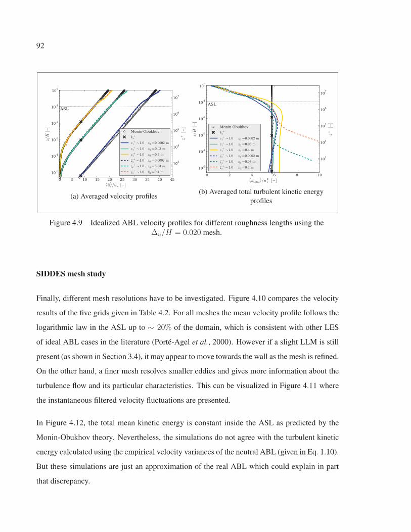
92

103

104

105

106

107

z+

[−]

10-5

10-4

10-3

10-2

10-1

100

z/H

[−]

0 5 10 15 20 25 30 35 40 45⟨u⟩/u

∗[−]

ASL

Monin-Obukhov

k +s

z +1 ∼1.0 z0 =0.0002 m

z +1 ∼1.0 z0 =0.03 m

z +1 ∼1.0 z0 =0.4 m

ζ +1 ∼1.0 z0 =0.0002 m

ζ +1 ∼1.0 z0 =0.03 m

ζ +1 ∼1.0 z0 =0.4 m

(a) Averaged velocity profiles

103

104

105

106

107

z+

[−]

10-5

10-4

10-3

10-2

10-1

100

z/H

[−]

0 2 4 6 8 10⟨ktotal

⟩/u 2

∗[−]

ASL

Monin-Obukhov

k +s

z +1 ∼1.0 z0 =0.0002 m

z +1 ∼1.0 z0 =0.03 m

z +1 ∼1.0 z0 =0.4 m

ζ +1 ∼1.0 z0 =0.0002 m

ζ +1 ∼1.0 z0 =0.03 m

ζ +1 ∼1.0 z0 =0.4 m

(b) Averaged total turbulent kinetic energy

profiles

Figure 4.9 Idealized ABL velocity profiles for different roughness lengths using the

Δu/H = 0.020 mesh.

SIDDES mesh study

Finally, different mesh resolutions have to be investigated. Figure 4.10 compares the velocity

results of the five grids given in Table 4.2. For all meshes the mean velocity profile follows the

logarithmic law in the ASL up to ∼ 20% of the domain, which is consistent with other LES

of ideal ABL cases in the literature (Porté-Agel et al., 2000). However if a slight LLM is still

present (as shown in Section 3.4), it may appear to move towards the wall as the mesh is refined.

On the other hand, a finer mesh resolves smaller eddies and gives more information about the

turbulence flow and its particular characteristics. This can be visualized in Figure 4.11 where

the instantaneous filtered velocity fluctuations are presented.

In Figure 4.12, the total mean kinetic energy is constant inside the ASL as predicted by the

Monin-Obukhov theory. Nevertheless, the simulations do not agree with the turbulent kinetic

energy calculated using the empirical velocity variances of the neutral ABL (given in Eq. 1.10).

But these simulations are just an approximation of the real ABL which could explain in part

that discrepancy.

93

105

106

107

z+

[−]

10-3

10-2

10-1

100

z/H

[−]

0 5 10 15 20 25⟨u⟩/u

∗[−]

ASL

Monin-Obukhov

k +s

Porte-Agel et al.(2000)

Δu /H=0.0250

Δu /H=0.0200

Δu /H=0.0150

Δu /H=0.0125

Δu /H=0.0100

Figure 4.10 Averaged velocity profiles for ideal ABL simulations with

the SIDDES model and a z0 = 0.1 m for different mesh resolutions.

Porté-Agel et al. (2000) data corresponds to the standard dynamic

Smagorinsky model results from such article.

The turbulent kinetic energy obtained by a hybrid model is also highly dependent on the mesh

resolution as well as the distance to the solid wall as expected. The modelled and resolved

components of the turbulent kinetic energy for two different resolutions are presented in Fig-

ure 4.13. The modelled turbulent kinetic energy k predominates close to the wall and it is

negligible far from it. It is crucial to be aware that the value of k depends on the k − ω SST

model constants. On the other hand, the resolved component k behaves in the opposite manner,

and the model constants do not have a direct impact on its value. It can also be observed that

k starts to increase or developed closer to the wall for the finer mesh. This same phenomenon

can also be verified in Figure 4.14 which displays the variance of each velocity component.

From here it can be deducted that the velocity fluctuations tend to zero close to the wall, but

they start to developed away from it. Additionally, it can be see that the finer mesh velocity

variance results are in closer agreement than the coarsest mesh.

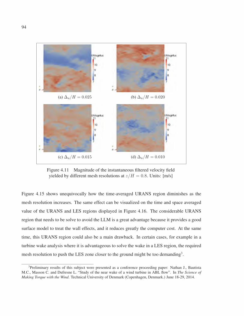
94

(a) Δu/H = 0.025 (b) Δu/H = 0.020

(c) Δu/H = 0.015 (d) Δu/H = 0.010

Figure 4.11 Magnitude of the instantaneous filtered velocity field

yielded by different mesh resolutions at z/H = 0.8. Units: [m/s]

Figure 4.15 shows unequivocally how the time-averaged URANS region diminishes as the

mesh resolution increases. The same effect can be visualized on the time and space averaged

value of the URANS and LES regions displayed in Figure 4.16. The considerable URANS

region that needs to be solve to avoid the LLM is a great advantage because it provides a good

surface model to treat the wall effects, and it reduces greatly the computer cost. At the same

time, this URANS region could also be a main drawback. In certain cases, for example in a

turbine wake analysis where it is advantageous to solve the wake in a LES region, the required

mesh resolution to push the LES zone closer to the ground might be too demanding3.

3Preliminary results of this subject were presented as a conference proceeding paper: Nathan J., Bautista

M.C., Masson C. and Dufresne L. “Study of the near wake of a wind turbine in ABL flow”. In The Science ofMaking Torque with the Wind. Technical University of Denmark (Copenhagen, Denmark.) June 18-29, 2014.

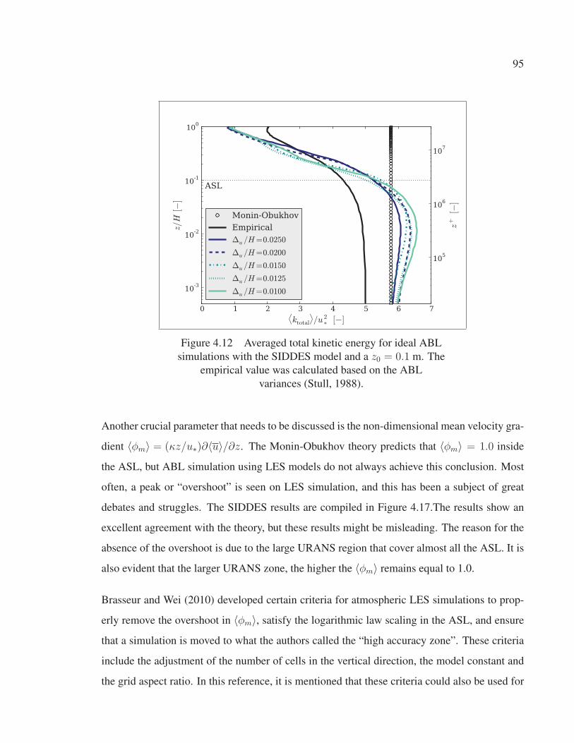
95

105

106

107

z+

[−]

10-3

10-2

10-1

100

z/H

[−]

0 1 2 3 4 5 6 7⟨ktotal

⟩/u 2

∗[−]

ASL

Monin-Obukhov

Empirical

Δu /H=0.0250

Δu /H=0.0200

Δu /H=0.0150

Δu /H=0.0125

Δu /H=0.0100

Figure 4.12 Averaged total kinetic energy for ideal ABL

simulations with the SIDDES model and a z0 = 0.1 m. The

empirical value was calculated based on the ABL

variances (Stull, 1988).

Another crucial parameter that needs to be discussed is the non-dimensional mean velocity gra-

dient 〈φm〉 = (κz/u∗)∂〈u〉/∂z. The Monin-Obukhov theory predicts that 〈φm〉 = 1.0 inside

the ASL, but ABL simulation using LES models do not always achieve this conclusion. Most

often, a peak or “overshoot” is seen on LES simulation, and this has been a subject of great

debates and struggles. The SIDDES results are compiled in Figure 4.17.The results show an

excellent agreement with the theory, but these results might be misleading. The reason for the

absence of the overshoot is due to the large URANS region that cover almost all the ASL. It is

also evident that the larger URANS zone, the higher the 〈φm〉 remains equal to 1.0.

Brasseur and Wei (2010) developed certain criteria for atmospheric LES simulations to prop-

erly remove the overshoot in 〈φm〉, satisfy the logarithmic law scaling in the ASL, and ensure

that a simulation is moved to what the authors called the “high accuracy zone”. These criteria

include the adjustment of the number of cells in the vertical direction, the model constant and

the grid aspect ratio. In this reference, it is mentioned that these criteria could also be used for

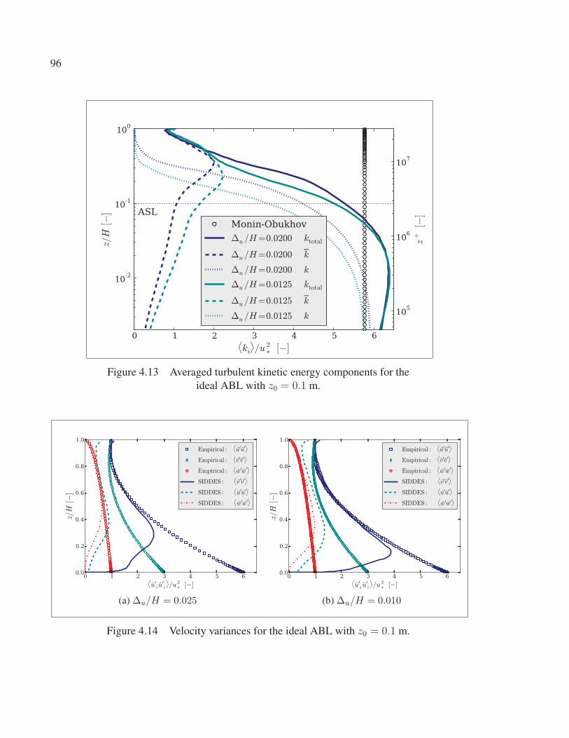
96

105

106

107

z+

[−]

10-2

10-1

100

z/H

[−]

0 1 2 3 4 5 6⟨ki⟩/u 2

∗[−]

ASL

Monin-Obukhov

Δu /H=0.0200 ktotal

Δu /H=0.0200 k

Δu /H=0.0200 k

Δu /H=0.0125 ktotal

Δu /H=0.0125 k

Δu /H=0.0125 k

Figure 4.13 Averaged turbulent kinetic energy components for the

ideal ABL with z0 = 0.1 m.

0 1 2 3 4 5 6⟨u′i u

′

i

⟩/u 2

∗[−]

0.0

0.2

0.4

0.6

0.8

1.0

z/H

[−]

Empirical :⟨u′u′

⟩

Empirical :⟨v′v′

⟩

Empirical :⟨w′w′

⟩

SIDDES :⟨v′v′

⟩

SIDDES :⟨u′u′

⟩

SIDDES :⟨w′w′

⟩

(a) Δu/H = 0.025

0 1 2 3 4 5 6⟨u′i u

′

i

⟩/u 2

∗[−]

0.0

0.2

0.4

0.6

0.8

1.0

z/H

[−]

Empirical :⟨u′u′

⟩

Empirical :⟨v′v′

⟩

Empirical :⟨w′w′

⟩

SIDDES :⟨v′v′

⟩

SIDDES :⟨u′u′

⟩

SIDDES :⟨w′w′

⟩

(b) Δu/H = 0.010

Figure 4.14 Velocity variances for the ideal ABL with z0 = 0.1 m.

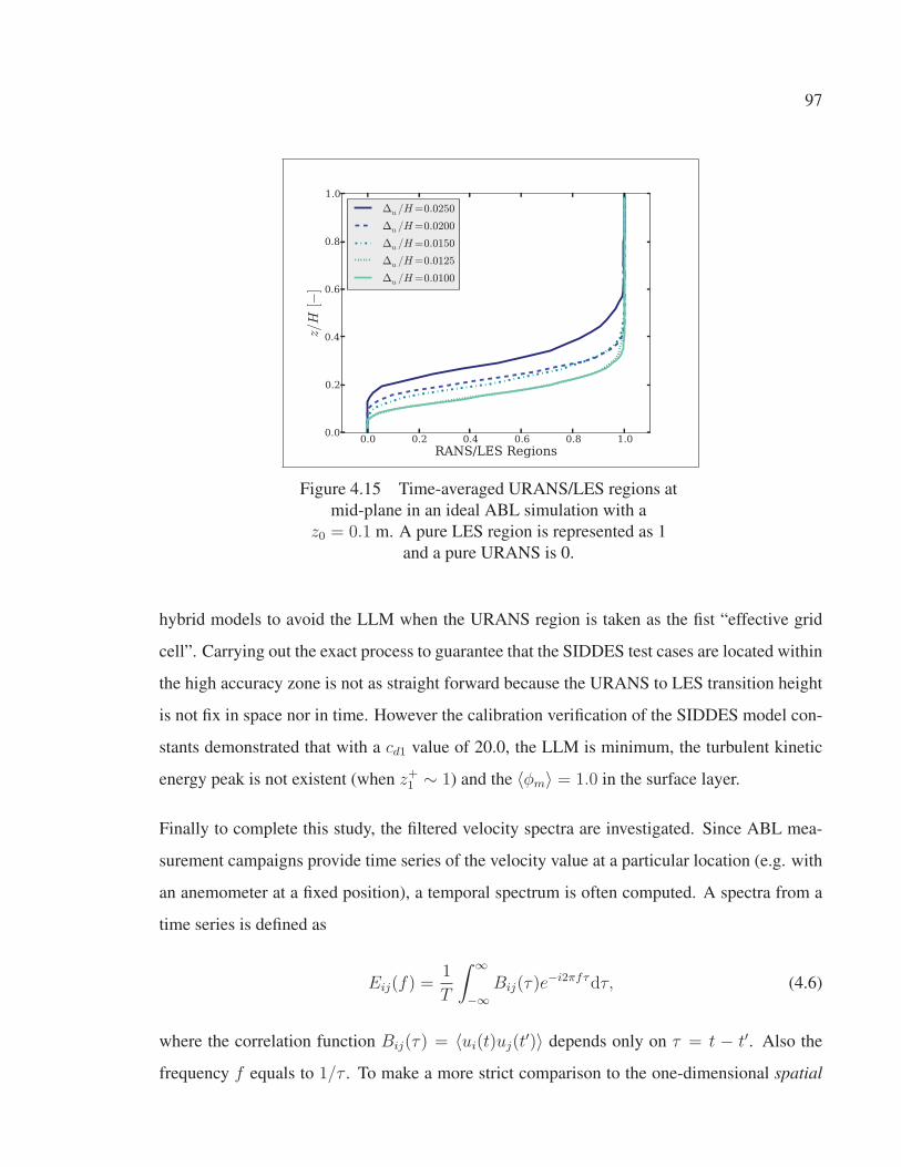
97

0.0 0.2 0.4 0.6 0.8 1.0

RANS/LES Regions

0.0

0.2

0.4

0.6

0.8

1.0

z/H

[−]

Δu /H=0.0250

Δu /H=0.0200

Δu /H=0.0150

Δu /H=0.0125

Δu /H=0.0100

Figure 4.15 Time-averaged URANS/LES regions at

mid-plane in an ideal ABL simulation with a

z0 = 0.1 m. A pure LES region is represented as 1

and a pure URANS is 0.

hybrid models to avoid the LLM when the URANS region is taken as the fist “effective grid

cell”. Carrying out the exact process to guarantee that the SIDDES test cases are located within

the high accuracy zone is not as straight forward because the URANS to LES transition height

is not fix in space nor in time. However the calibration verification of the SIDDES model con-

stants demonstrated that with a cd1 value of 20.0, the LLM is minimum, the turbulent kinetic

energy peak is not existent (when z+1 ∼ 1) and the 〈φm〉 = 1.0 in the surface layer.

Finally to complete this study, the filtered velocity spectra are investigated. Since ABL mea-

surement campaigns provide time series of the velocity value at a particular location (e.g. with

an anemometer at a fixed position), a temporal spectrum is often computed. A spectra from a

time series is defined as

Eij(f) =1

T

∫ ∞

−∞Bij(τ)e

−i2πfτdτ, (4.6)

where the correlation function Bij(τ) = 〈ui(t)uj(t′)〉 depends only on τ = t − t′. Also the

frequency f equals to 1/τ . To make a more strict comparison to the one-dimensional spatial

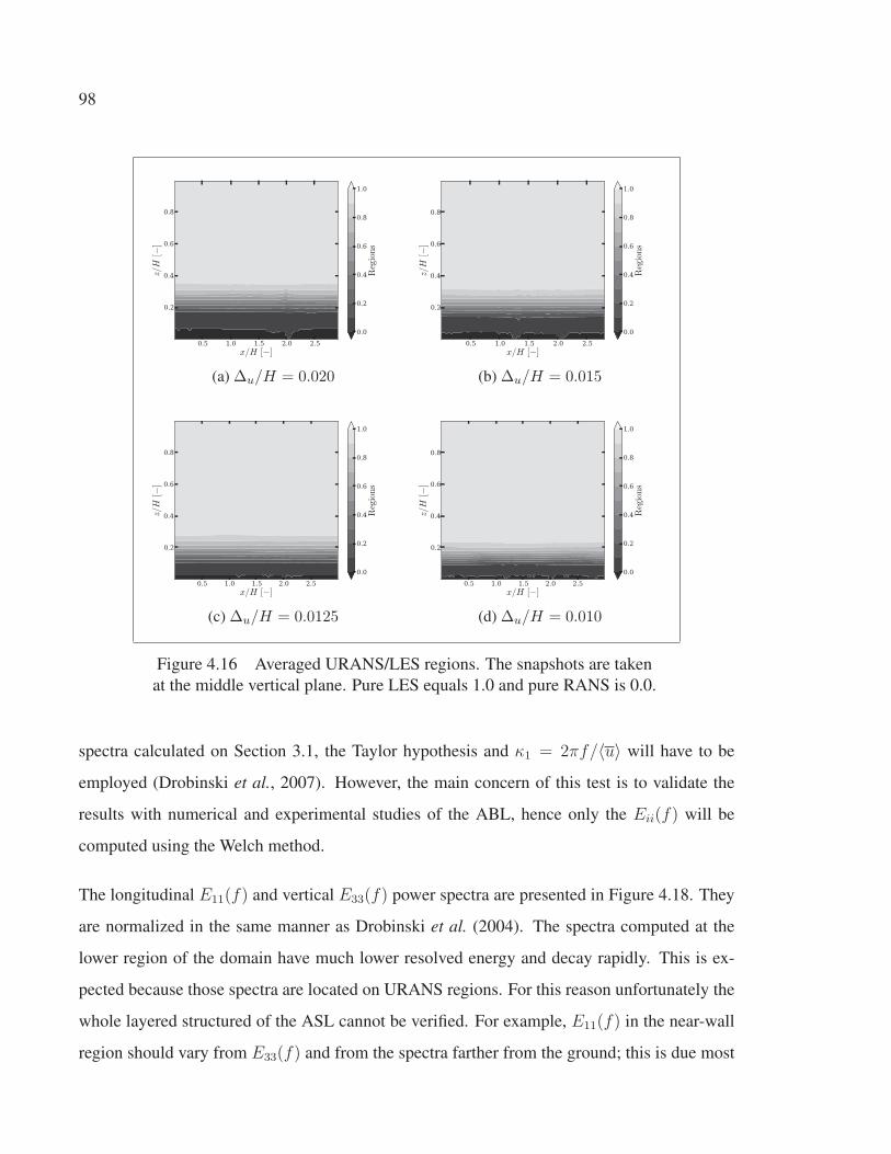
98

0.5 1.0 1.5 2.0 2.5

x/H [−]

0.2

0.4

0.6

0.8

z/H

[−]

0.0

0.2

0.4

0.6

0.8

1.0

Reg

ions

(a) Δu/H = 0.020

0.5 1.0 1.5 2.0 2.5

x/H [−]

0.2

0.4

0.6

0.8

z/H

[−]

0.0

0.2

0.4

0.6

0.8

1.0

Reg

ions

(b) Δu/H = 0.015

0.5 1.0 1.5 2.0 2.5

x/H [−]

0.2

0.4

0.6

0.8

z/H

[−]

0.0

0.2

0.4

0.6

0.8

1.0

Reg

ions

(c) Δu/H = 0.0125

0.5 1.0 1.5 2.0 2.5

x/H [−]

0.2

0.4

0.6

0.8

z/H

[−]

0.0

0.2

0.4

0.6

0.8

1.0

Reg

ions

(d) Δu/H = 0.010

Figure 4.16 Averaged URANS/LES regions. The snapshots are taken

at the middle vertical plane. Pure LES equals 1.0 and pure RANS is 0.0.

spectra calculated on Section 3.1, the Taylor hypothesis and κ1 = 2πf/〈u〉 will have to be

employed (Drobinski et al., 2007). However, the main concern of this test is to validate the

results with numerical and experimental studies of the ABL, hence only the Eii(f) will be

computed using the Welch method.

The longitudinal E11(f) and vertical E33(f) power spectra are presented in Figure 4.18. They

are normalized in the same manner as Drobinski et al. (2004). The spectra computed at the

lower region of the domain have much lower resolved energy and decay rapidly. This is ex-

pected because those spectra are located on URANS regions. For this reason unfortunately the

whole layered structured of the ASL cannot be verified. For example, E11(f) in the near-wall

region should vary from E33(f) and from the spectra farther from the ground; this is due most

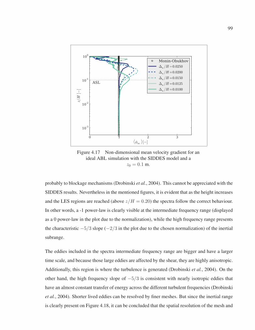
99

10-3

10-2

10-1

100

z/H

[−]

0 1 2 3⟨φm

⟩[−]

ASL

Monin-Obukhov

Δu /H=0.0250

Δu /H=0.0200

Δu /H=0.0150

Δu /H=0.0125

Δu /H=0.0100

Figure 4.17 Non-dimensional mean velocity gradient for an

ideal ABL simulation with the SIDDES model and a

z0 = 0.1 m.

probably to blockage mechanisms (Drobinski et al., 2004). This cannot be appreciated with the

SIDDES results. Nevertheless in the mentioned figures, it is evident that as the height increases

and the LES regions are reached (above z/H = 0.20) the spectra follow the correct behaviour.

In other words, a -1 power-law is clearly visible at the intermediate frequency range (displayed

as a 0 power-law in the plot due to the normalization), while the high frequency range presents

the characteristic −5/3 slope (−2/3 in the plot due to the chosen normalization) of the inertial

subrange.

The eddies included in the spectra intermediate frequency range are bigger and have a larger

time scale, and because those large eddies are affected by the shear, they are highly anisotropic.

Additionally, this region is where the turbulence is generated (Drobinski et al., 2004). On the

other hand, the high frequency slope of −5/3 is consistent with nearly isotropic eddies that

have an almost constant transfer of energy across the different turbulent frequencies (Drobinski

et al., 2004). Shorter lived eddies can be resolved by finer meshes. But since the inertial range

is clearly present on Figure 4.18, it can be concluded that the spatial resolution of the mesh and

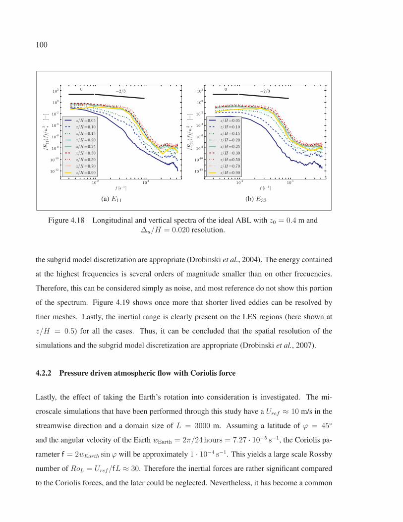
100

10-2

10-1

f [s−1 ]

10-12

10-10

10-8

10-6

10-4

10-2

100

102

fE11(f)/u

2 ∗[−

]

−2/30

z/H=0.05

z/H=0.10

z/H=0.15

z/H=0.20

z/H=0.25

z/H=0.30

z/H=0.50

z/H=0.70

z/H=0.90

(a) E11

10-2

10-1

f [s−1 ]

10-12

10-10

10-8

10-6

10-4

10-2

100

102

fE33(f)/u

2 ∗[−

]

−2/30

z/H=0.05

z/H=0.10

z/H=0.15

z/H=0.20

z/H=0.25

z/H=0.30

z/H=0.50

z/H=0.70

z/H=0.90

(b) E33

Figure 4.18 Longitudinal and vertical spectra of the ideal ABL with z0 = 0.4 m and

Δu/H = 0.020 resolution.

the subgrid model discretization are appropriate (Drobinski et al., 2004). The energy contained

at the highest frequencies is several orders of magnitude smaller than on other frecuencies.

Therefore, this can be considered simply as noise, and most reference do not show this portion

of the spectrum. Figure 4.19 shows once more that shorter lived eddies can be resolved by

finer meshes. Lastly, the inertial range is clearly present on the LES regions (here shown at

z/H = 0.5) for all the cases. Thus, it can be concluded that the spatial resolution of the

simulations and the subgrid model discretization are appropriate (Drobinski et al., 2007).

4.2.2 Pressure driven atmospheric flow with Coriolis force

Lastly, the effect of taking the Earth’s rotation into consideration is investigated. The mi-

croscale simulations that have been performed through this study have a Uref ≈ 10 m/s in the

streamwise direction and a domain size of L = 3000 m. Assuming a latitude of ϕ = 45◦

and the angular velocity of the Earth wEarth = 2π/24 hours = 7.27 · 10−5 s−1, the Coriolis pa-

rameter f = 2wEarth sinϕ will be approximately 1 · 10−4 s−1. This yields a large scale Rossby

number of RoL = Uref/fL ≈ 30. Therefore the inertial forces are rather significant compared

to the Coriolis forces, and the later could be neglected. Nevertheless, it has become a common

101

10-2

10-1

f [s−1 ]

10-8

10-7

10-6

10-5

10-4

10-3

10-2

10-1

100

101

102

103

fE11(f)/u

2 ∗[−

]

−2/30

z/H=0.5

Δu /H=0.0250

Δu /H=0.0200

Δu /H=0.0150

Δu /H=0.0125

Δu /H=0.0100

Figure 4.19 Spectra from ideal ABL simulations with the

SIDDES model and a z0 = 0.1 m.

practice to include the rotation effects at a microscale level (e.g. Churchfield et al. (2014)),

possibly in an attempt to merge microscale and mesoscale software.

To include the Coriolis force in the ABL simulations two important steps have to be followed.

First the Coriolis force term FC = −2Ω × u has to be added to the momentum equation.

Here Ω = (0, wEarth cosϕ, wEarth sinϕ) represents the Earth’s angular velocity vector at a

latitude ϕ. Second the large scale pressure gradient term that drives the flow has to be adjusted

with respect to previous simulations. The computation of this driving pressure gradient is

once again calculated following the procedure shown in Section 3.4. But for a steady and

horizontally homogeneous flow that includes the Coriolis force, the hybrid model momentum

equations become

1

ρ

∂〈p〉∂x

=+ f〈v〉+ 1

ρ

∂〈τxz〉∂z

(4.7)

1

ρ

∂〈p〉∂y

=− f〈u〉+ 1

ρ

∂〈τ yz〉∂z

(4.8)

102

for the streamwise and spanwise direction respectively. This balance between pressure, Corio-

lis and frictional forces describe the Ekman layer. At the top of the atmosphere, the geostrophic

wind is the result of only the Coriolis and pressure forces, since at that height the frictional

forces are negligible. Following the procedure given in Bechmann (2006), this simplifies to

1

ρ

∂〈p〉∂x

=+ f〈vg〉 (4.9)

1

ρ

∂〈p〉∂y

=− f〈ug〉 (4.10)

Therefore for a geostrophic wind that drives the flow in the streamwise direction

(ug, vg, wg) = (ug, 0, 0), the large scale pressure gradient is given by

F =

(∂〈p〉∂x

,∂〈p〉∂y

,∂〈p〉∂z

)(4.11)

F =(0, −ρf〈ug〉, 0) (4.12)

When the Coriolis force is being considered at a microscale level only some minor differences

are perceived. Figure 4.20 shows two simulations with and without Coriolis forces. The choice

of mesh resolution for this simulations is not ideal, a better conclusion could have been reached

if a finer mesh had been used. In spite of this it can be observed that the spanwise velocity

is different than zero only for the Coriolis case, thus the Ekman layer forms. On the other

hand, the streamwise velocity component is not really affected. To emphasize this findings,

Figure 4.21 illustrates a snapshot of the velocity field at a certain height. If observed in detail,

it can be seen that the Coriolis case presents velocity streaks that are not aligned with the

streamwise direction, while this orientation offset is not visible in the case without Coriolis.

Also because of the large URANS zones, the near-wall streaks studied by Drobinski and Foster

(2003) could not be compared with this coarse mesh. Finally based in Section 3.2, it is expected

that the Earth’s rotation does not affect the turbulence statistics.

Results show that the roughness height is a relevant factor in the development of the Ekman

spiral. Figure 4.22 displays the averaged velocity profiles computed by simulations of the ABL

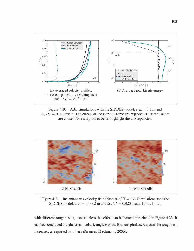
103

0 5 10 15 20 25⟨u⟩/u

∗[−]

0.0

0.2

0.4

0.6

0.8

1.0z/H

[−]

ASL

Monin-Obukhov

No Coriolis

With Coriolis

(a) Averaged velocity profiles.

−−: u-component, −. : v-component

and −: U =√u2 + v2.

105

106

107

z+

[−]

10-3

10-2

10-1

100

z/H

[−]

0 1 2 3 4 5 6 7⟨ktotal

⟩/u 2

∗[−]

ASL

Monin-Obukhov

k +s

No Coriolis

With Coriolis

(b) Averaged total kinetic energy

Figure 4.20 ABL simulations with the SIDDES model, a z0 = 0.4 m and

Δu/H = 0.020 mesh. The effects of the Coriolis force are explored. Different scales

are chosen for each plots to better highlight the discrepancies.

(a) No Coriolis (b) With Coriolis

Figure 4.21 Instantaneous velocity field taken at z/H = 0.8. Simulations used the

SIDDES model, a z0 = 0.0002 m and Δu/H = 0.020 mesh. Units: [m/s].

with different roughness z0, nevertheless this effect can be better appreciated in Figure 4.23. It

can bee concluded that the cross-isobaric angle θ of the Ekman spiral increases as the roughness

increases, as reported by other references (Bechmann, 2006).

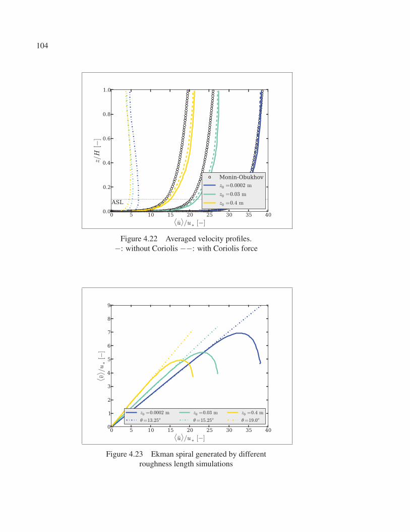
104

0 5 10 15 20 25 30 35 40⟨u⟩/u

∗[−]

0.0

0.2

0.4

0.6

0.8

1.0

z/H

[−]

ASL

Monin-Obukhov

z0 =0.0002 m

z0 =0.03 m

z0 =0.4 m

Figure 4.22 Averaged velocity profiles.

−: without Coriolis −−: with Coriolis force

0 5 10 15 20 25 30 35 40⟨u⟩/u

∗[−]

0

1

2

3

4

5

6

7

8

9

⟨ v⟩ /u∗[−

]

z0 =0.0002 m

θ=13.25oz0 =0.03 m

θ=15.25oz0 =0.4 m

θ=19.0o

Figure 4.23 Ekman spiral generated by different

roughness length simulations

105

4.3 Høvsøre field measurement campaign: neutral case

One of the most recent and complete field measurement campaign was carried out in Høvsøre,

Denmark (Peña et al., 2014). Accurate observations with modern instrumentation were per-

formed for a period of 1-year over nearly homogeneous flat terrain under various stratification

conditions. Peña et al. (2014) clearly indicates all the ABL conditions during each observation

period and it provides a thorough explanation of the data analysis. Additionally WRF (Weather

Research and Forecasting mesoscale model (The WRF community, 2015)) simulations were

performed for the different observed stratification cases. Such experimental measurement as

well as the WRF modelling results are accessible online. The neutral stratification case (refer

to Case 5 on the mentioned reference) is simulated using the k − ω SST-SIDDES hybrid mi-

croscale model. The comparison of the results will determine the accuracy of the hybrid model

implementation over a “real and full-scale” natural flat terrain.

The microscale simulation is performed on a domain of size of (Lx, Ly, Lz) = (3H, 3H, H)

where H = 1150 m. Such height is chosen to be consistent with the ABL height obtained

by the WRF simulation (i.e. 1120 m). Additionally the measured terrain roughness is

z0 = 0.015 m. The mesh contains about 8.2 · 106 cells and it follows the same meshing tech-

nique as the previous cases. The cells have an expansion ratio of 1.15 up to a height of

zu/H = 0.1, from there all the cells are cubic with a Δu/H = 0.013. The domain bound-

ary conditions are the same as for the previous flat terrain cases. The large scale driving

pressure gradient is calculated as on Section 4.2.2 based on the velocity measured at H , thus

(ug, vg) = (17.81, 7.83) m/s. Also a latitude of ϕ = 56.43◦ is used to calculate the Coriolis

factor. The velocity field is initiated with a logarithmic profile for the streamwise component,

a linear slope profile for the spanwise component, and some added random fluctuations on

all three components. Because the value of vg is non zero in this case, the initial spanwise

component is computed a bit differently than previously done. Thus the velocity streamwise

component was initiated with a logarithmic profile as before, but the spanwise component was

defined by a linear profile. Lastly, ±20% of random fluctuations were added to all three initial

velocity components.

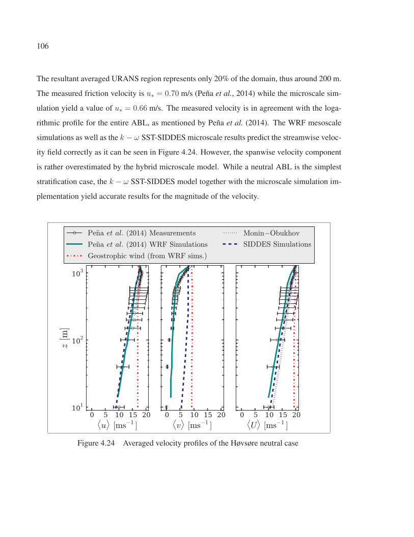
106

The resultant averaged URANS region represents only 20% of the domain, thus around 200 m.

The measured friction velocity is u∗ = 0.70 m/s (Peña et al., 2014) while the microscale sim-

ulation yield a value of u∗ = 0.66 m/s. The measured velocity is in agreement with the loga-

rithmic profile for the entire ABL, as mentioned by Peña et al. (2014). The WRF mesoscale

simulations as well as the k − ω SST-SIDDES microscale results predict the streamwise veloc-

ity field correctly as it can be seen in Figure 4.24. However, the spanwise velocity component

is rather overestimated by the hybrid microscale model. While a neutral ABL is the simplest

stratification case, the k − ω SST-SIDDES model together with the microscale simulation im-

plementation yield accurate results for the magnitude of the velocity.

0 5 10 15 20⟨u

⟩[ms−1 ]

101

102

103

z[m

]

0 5 10 15 20⟨v

⟩[ms−1 ]

0 5 10 15 20⟨U

⟩[ms−1 ]

Pena et al. (2014) Measurements

Pena et al. (2014) WRF Simulations

Geostrophic wind (from WRF sims.)

Monin−Obukhov

SIDDES Simulations

Figure 4.24 Averaged velocity profiles of the Høvsøre neutral case

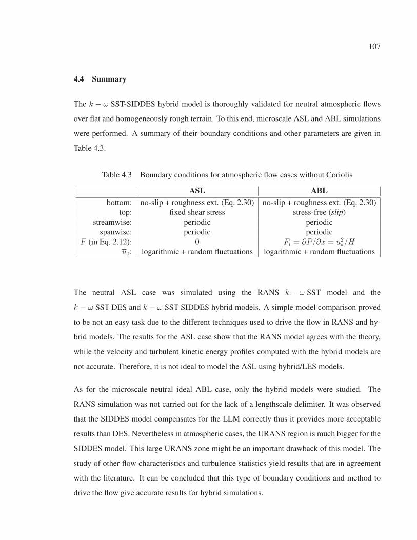
107

4.4 Summary

The k − ω SST-SIDDES hybrid model is thoroughly validated for neutral atmospheric flows

over flat and homogeneously rough terrain. To this end, microscale ASL and ABL simulations

were performed. A summary of their boundary conditions and other parameters are given in

Table 4.3.

Table 4.3 Boundary conditions for atmospheric flow cases without Coriolis

ASL ABLbottom: no-slip + roughness ext. (Eq. 2.30) no-slip + roughness ext. (Eq. 2.30)

top: fixed shear stress stress-free (slip)

streamwise: periodic periodic

spanwise: periodic periodic

F (in Eq. 2.12): 0 Fi = ∂P/∂x = u2∗/H

u0: logarithmic + random fluctuations logarithmic + random fluctuations

The neutral ASL case was simulated using the RANS k − ω SST model and the

k − ω SST-DES and k − ω SST-SIDDES hybrid models. A simple model comparison proved

to be not an easy task due to the different techniques used to drive the flow in RANS and hy-

brid models. The results for the ASL case show that the RANS model agrees with the theory,

while the velocity and turbulent kinetic energy profiles computed with the hybrid models are

not accurate. Therefore, it is not ideal to model the ASL using hybrid/LES models.

As for the microscale neutral ideal ABL case, only the hybrid models were studied. The

RANS simulation was not carried out for the lack of a lengthscale delimiter. It was observed

that the SIDDES model compensates for the LLM correctly thus it provides more acceptable

results than DES. Nevertheless in atmospheric cases, the URANS region is much bigger for the

SIDDES model. This large URANS zone might be an important drawback of this model. The

study of other flow characteristics and turbulence statistics yield results that are in agreement

with the literature. It can be concluded that this type of boundary conditions and method to

drive the flow give accurate results for hybrid simulations.

108

The k − ω SST-SIDDES model behaviour is better understood as a result of the flat terrain

study. It has been demonstrated that the hybrid model captures the correct features of a sim-

plified atmosphere model when the Coriolis effects are neglected and when they are included.

Additionally, it has been verified that the hybrid model yields results of the velocity magni-

tude which are in agreement with the neutral case of the Høvsøre measurement campaign and

WRF simulations. Nevertheless, the major achievement of this analysis is the development of

a turbulence model with the following characteristics:

• The wall treatment is less dependent on flat terrain assumptions (i.e. no wall function

required nor a velocity or a shear value is imposed to the first cell)

• The description of the turbulent flow that could be attained is more detailed and complete

due to the LES methodology.

• The computer cost might be reduced without highly compromising the accuracy of the

results because of the hybrid approach.

Consequently the SIDDES hybrid model based on the k−ω SST equations is expected to be a

good candidate for complex terrain simulations.

CHAPTER 5

MICROSCALE ATMOSPHERIC FLOW SIMULATIONS OVER COMPLEXTOPOGRAPHY

To conclude the analysis of the ABL using the hybrid model k − ω SST-SIDDES, the flow

behaviour will be studied over complex terrain. When heterogeneous terrain or an obstacle is

modelled, the boundary conditions on the streamwise direction need to be redefined. Contrary

to the flat terrain cases, a simple periodic condition might not be accurate for complex terrain

cases. An obstacle will most likely influence the nature of the flow for a considerable distance

far downstream. Then if periodic boundaries are used and the domain is not sufficiently long,

the effects of the obstacle will be wrongly reintroduce at the inlet. Alternatively an inlet profile

and an outlet boundary condition have to be defined.

A simple mean logarithmic profile at the domain entrance is not sufficient for LES test cases.

Inlet flows must include the unsteady and turbulent flow behaviour, as well as other special

considerations to reproduce the natural characteristics of the wind (Uchida and Ohya, 2003).

Numerous methods exist to generate these realistic inflows. For instance, randomly gener-

ating isotropic fluctuations in the velocity components and adding them to the mean veloc-

ity profile at the inlet (Troldborg, 2008), increasing the computational domain and defining

buffer zones between the inlet and the region of interest to allow for the flow to become tur-

bulent (Uchida and Ohya, 2003), or using a precursor simulation (e.g. Bechmann (2006) or as

done by Churchfield et al. (2014)). This latest method computes first a streamwise periodic

simulation of the wind flow over flat terrain, then for every time step, the resulting flow field at

a particular plane is mapped to the inlet of the complex terrain simulation (Castro et al., 2003).

A simple analysis of some methods to generate an inflow will be done.

Neumann boundary conditions will be used for the outlet, meaning that ∂φ/∂x = 0 for any

variable φ. Then in order to avoid having a singular solution, the value of the pressure must be

set at a certain location. However, it has been observed (e.g. (Bechmann, 2006)) that this type

of condition could sometimes yield a non-physical flow behaviour near the outlet. Another

110

solution can be to increase the computational domain and simply disregard a buffer zone close

to the outlet, or to apply a convective outflow (Uchida and Ohya, 2003).

The complex terrain analysis will include the simulation of simplified test cases that represent

idealized complex terrains. Typically such simplified cases are carried out experimentally in a

wind-tunnel and include detailed measurements of the flow characteristics. Thus, a thorough

comparison of the fluid behaviour in the experimental measurements and the modelling results

can be done. Nevertheless quantifying the error and uncertainties of those comparisons is not

simple (Oberkampf and Trucano, 2002).

Lastly, the final challenge is to use the hybrid turbulence model to predict the actual three

dimensional complex flow induced by a full scale terrain. The wind industry uses field mea-

surements, like the ones taken at Askervein hill in Scotland (1982-1983) (Salmon et. al., 1988)

and the peninsula of Bolund in Denmark (2007-2008) (Berg et al., 2011) as reference real

validation test cases. Nevertheless, the data obtained in a field campaign is not as detailed as

the ones from a wind-tunnel experiment. In real terrain, a couple measuring masts are placed

strategically at different places and at different heights, but the horizontal and vertical resolu-

tion of this data is very limited. Based on so few data points, it is hard to critically qualify the

performance of a turbulence model; nevertheless, it is now the only viable option to validate

real terrain.

Following all these considerations, the simplified test case of square-section cylinder will be

modelled. This case was chosen mainly because of the detailed and recent wind-tunnel mea-

surements that are available for comparison. Lastly, a simulation of the Askervein hill case will

be carried out and compare against measurement obtained in full scale complex terrain.

5.1 Flow around a square-section cylinder

Complex phenomena arises when a fluid encounters an obstacle like a 3D square-section cylin-

der mounted on a smooth surface. The flow can exhibit unsteadiness, separation and reattach-

ment points, wake formation, vortex shedding, and a non-trivial wall interaction that entails

111

significant challenges for the numerical simulations. Several experiments have shown that the

nature of the flow and wake formation depends on the Reynolds number (Lim et al., 2007), the

surfaces condition (Lim et al., 2009) and aspect ratio of the square-section cylinder (Sakamoto,

1983), as well as the characteristics of the approaching flow (i.e. the turbulence intensity and

the boundary layer height relative to the obstacle height) (Castro and Robins, 1977; Wang et al.,

2006).

Numerous attempts to model the flow around other similar square cylinder cases have been

carried out using different turbulence models, but the results are not been fully consistent with

the experimental measurements (Sagaut, 2006). In this section, numerical simulations of the

flow around a square-section cylinder are undertaken. The focus of these simulations is not

be to carry out a complete and through comparison against all the available experimental re-

sults. Instead, the purpose is simply to verify if the hybrid model can reproduce some of the

phenomena already seen by the mentioned authors.

The numerical simulations were defined based on the CFD Society of Canada 2012/2013

Challenge wind-tunnel experiment (http://www.cfdcanada.ca/challenge). The details about the

experimental setup and results can be found on Bourgeois et al. (2011) and Sattari et al.

(2011). Essentially the computational case-study includes a square cylinder with a cross-

section of d = 12.7mm and a height of h = 50.4mm (aspect ratio h/d ≈ 4). The domain size

is (Lx, Ly, Lz) = (9h, 4h, 3h) which represent the streamwise, spanwise and vertical direc-

tions, respectively. The mesh is centred at the obstacle which is placed at a distance of 4h from

the inlet. In order to better reproduce the turbulent flow, and at the same time, to save on com-

puting cost, the grid is divided in three regions with different refinements as seen in Figure 5.1.

Therefore, close to the wall and the obstacle, and in the wake formation zone the cells are

smaller in size. Additionally, four layers of cells with an expansion ratio of Δzi+1/Δzi = 1.15

where added close to the bottom and obstacle walls. z represents the perpendicular direction to

the nearest wall; thus a vertical refinement is set close to the bottom wall and the top face of

the obstacle, and a streamwise and spanwise refinement is imposed around the obstacle sides.

The purpose of these layers is to attain as much as possible the z+1 = z1u∗/ν ≈ 1 as required by

112

k − ω SST for smooth walls (Knopp et al., 2009), where u∗ is the friction velocity, and z1 is the

perpendicular distance from any wall to the nearest cell centre. Most cell are cubic following

the mesh guidelines for DES (Spalart, 2001), except in the interface between the refinement

regions and close to the walls. These meshing procedure yields a mesh with approximately

1 ·106 cells. The number of cells might not be notable with current computers resources. How-

ever attaining the z+1 ≈ 1 posses a great challenge for the mesh generator in particular at the

square cylinder edges. For this reason around the obstacle, the z+1 requirement was relaxed to

around 10 to avoid faulty meshes (due to the limitations of the mesh generator). While z+1 was

relaxed up to 2 in the bottom wall. A CFL of 0.7 was used. Lastly, no space averages can be

computed in complex terrain cases. In this chapter 〈·〉 represents a time-averaged value only.

Figure 5.1 Vertical plane of the mesh with three refinement regions. Layers of

cells were added close the bottom and obstacle walls to achieve a smaller z+1 .

The wind-tunnel experiment was carried out with an upstream thin boundary layer flow, in

other words, the approaching flow presents a boundary layer which is small compared to the

size of the obstacle (δ < h). This is an ideal case to validate the performance of the hybrid

models within its original formulation (i.e. solving only the boundary layer with URANS, and

using LES everywhere else); but at the same time, this is hardly the case in ABL flows where

most likely δ > h. A proper hybrid model validation will require an experiment that comprises

measurements where the approaching boundary layer height is small relative to the obstacle

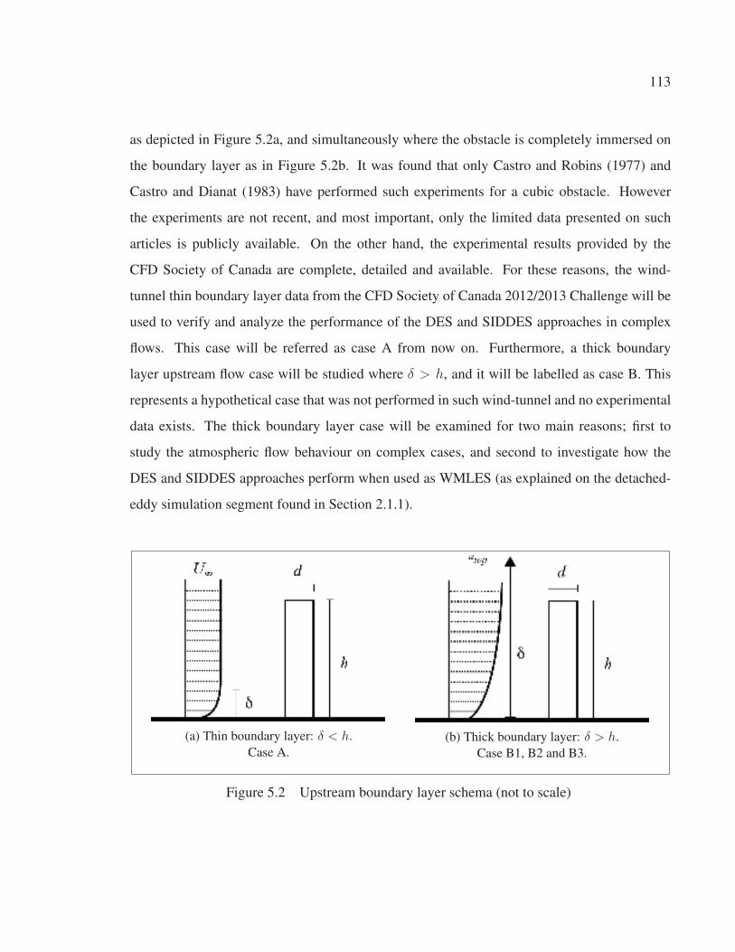
113

as depicted in Figure 5.2a, and simultaneously where the obstacle is completely immersed on

the boundary layer as in Figure 5.2b. It was found that only Castro and Robins (1977) and

Castro and Dianat (1983) have performed such experiments for a cubic obstacle. However

the experiments are not recent, and most important, only the limited data presented on such

articles is publicly available. On the other hand, the experimental results provided by the

CFD Society of Canada are complete, detailed and available. For these reasons, the wind-

tunnel thin boundary layer data from the CFD Society of Canada 2012/2013 Challenge will be

used to verify and analyze the performance of the DES and SIDDES approaches in complex

flows. This case will be referred as case A from now on. Furthermore, a thick boundary

layer upstream flow case will be studied where δ > h, and it will be labelled as case B. This

represents a hypothetical case that was not performed in such wind-tunnel and no experimental

data exists. The thick boundary layer case will be examined for two main reasons; first to

study the atmospheric flow behaviour on complex cases, and second to investigate how the

DES and SIDDES approaches perform when used as WMLES (as explained on the detached-

eddy simulation segment found in Section 2.1.1).

(a) Thin boundary layer: δ < h.

Case A.

(b) Thick boundary layer: δ > h.

Case B1, B2 and B3.

Figure 5.2 Upstream boundary layer schema (not to scale)

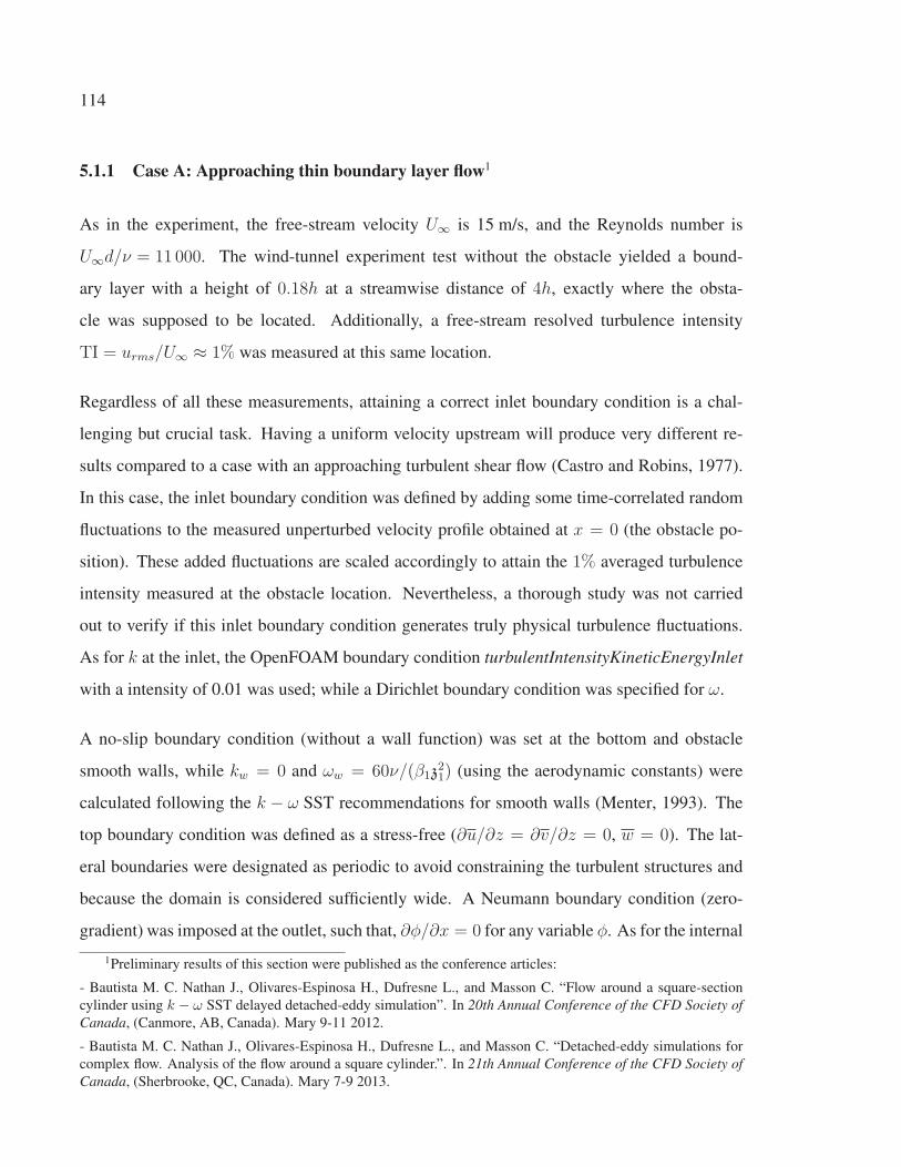
114

5.1.1 Case A: Approaching thin boundary layer flow1

As in the experiment, the free-stream velocity U∞ is 15 m/s, and the Reynolds number is

U∞d/ν = 11 000. The wind-tunnel experiment test without the obstacle yielded a bound-

ary layer with a height of 0.18h at a streamwise distance of 4h, exactly where the obsta-

cle was supposed to be located. Additionally, a free-stream resolved turbulence intensity

TI = urms/U∞ ≈ 1% was measured at this same location.

Regardless of all these measurements, attaining a correct inlet boundary condition is a chal-

lenging but crucial task. Having a uniform velocity upstream will produce very different re-

sults compared to a case with an approaching turbulent shear flow (Castro and Robins, 1977).

In this case, the inlet boundary condition was defined by adding some time-correlated random

fluctuations to the measured unperturbed velocity profile obtained at x = 0 (the obstacle po-

sition). These added fluctuations are scaled accordingly to attain the 1% averaged turbulence

intensity measured at the obstacle location. Nevertheless, a thorough study was not carried

out to verify if this inlet boundary condition generates truly physical turbulence fluctuations.

As for k at the inlet, the OpenFOAM boundary condition turbulentIntensityKineticEnergyInlet

with a intensity of 0.01 was used; while a Dirichlet boundary condition was specified for ω.

A no-slip boundary condition (without a wall function) was set at the bottom and obstacle

smooth walls, while kw = 0 and ωw = 60ν/(β1z21) (using the aerodynamic constants) were

calculated following the k − ω SST recommendations for smooth walls (Menter, 1993). The

top boundary condition was defined as a stress-free (∂u/∂z = ∂v/∂z = 0, w = 0). The lat-

eral boundaries were designated as periodic to avoid constraining the turbulent structures and

because the domain is considered sufficiently wide. A Neumann boundary condition (zero-

gradient) was imposed at the outlet, such that, ∂φ/∂x = 0 for any variable φ. As for the internal

1Preliminary results of this section were published as the conference articles:

- Bautista M. C. Nathan J., Olivares-Espinosa H., Dufresne L., and Masson C. “Flow around a square-section

cylinder using k − ω SST delayed detached-eddy simulation”. In 20th Annual Conference of the CFD Society ofCanada, (Canmore, AB, Canada). Mary 9-11 2012.

- Bautista M. C. Nathan J., Olivares-Espinosa H., Dufresne L., and Masson C. “Detached-eddy simulations for

complex flow. Analysis of the flow around a square cylinder.”. In 21th Annual Conference of the CFD Society ofCanada, (Sherbrooke, QC, Canada). Mary 7-9 2013.

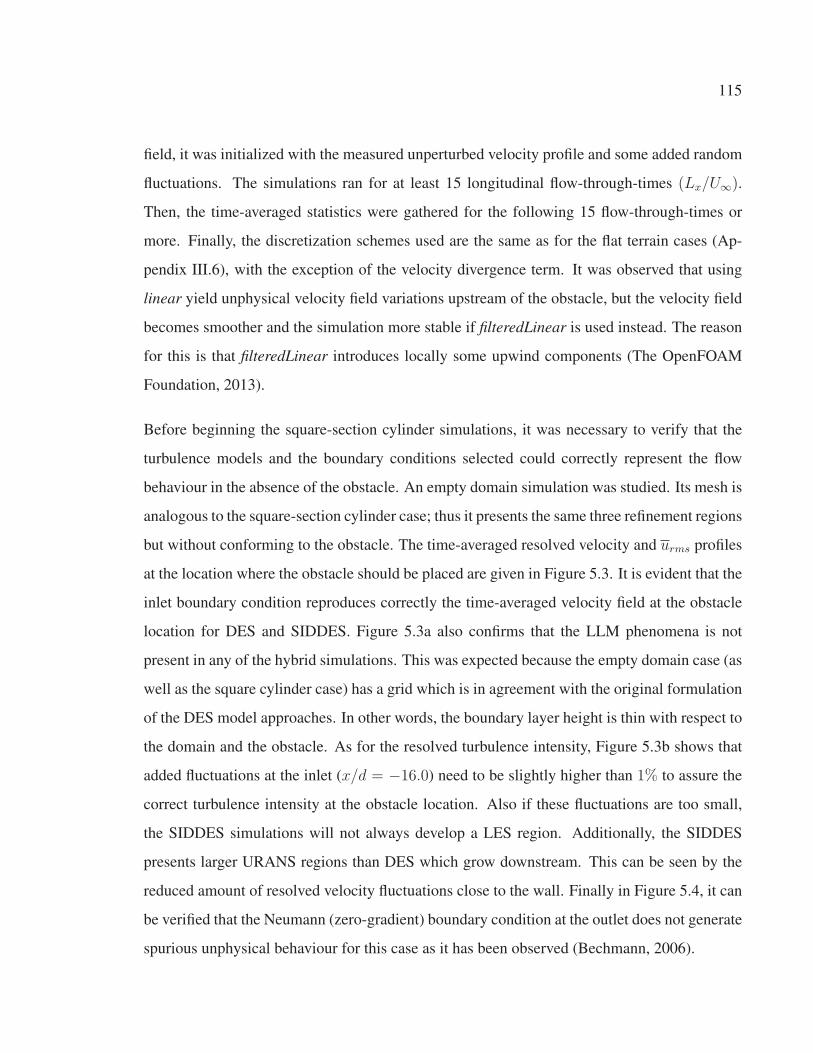
115

field, it was initialized with the measured unperturbed velocity profile and some added random

fluctuations. The simulations ran for at least 15 longitudinal flow-through-times (Lx/U∞).

Then, the time-averaged statistics were gathered for the following 15 flow-through-times or

more. Finally, the discretization schemes used are the same as for the flat terrain cases (Ap-

pendix III.6), with the exception of the velocity divergence term. It was observed that using

linear yield unphysical velocity field variations upstream of the obstacle, but the velocity field

becomes smoother and the simulation more stable if filteredLinear is used instead. The reason

for this is that filteredLinear introduces locally some upwind components (The OpenFOAM

Foundation, 2013).

Before beginning the square-section cylinder simulations, it was necessary to verify that the

turbulence models and the boundary conditions selected could correctly represent the flow

behaviour in the absence of the obstacle. An empty domain simulation was studied. Its mesh is

analogous to the square-section cylinder case; thus it presents the same three refinement regions

but without conforming to the obstacle. The time-averaged resolved velocity and urms profiles

at the location where the obstacle should be placed are given in Figure 5.3. It is evident that the

inlet boundary condition reproduces correctly the time-averaged velocity field at the obstacle

location for DES and SIDDES. Figure 5.3a also confirms that the LLM phenomena is not

present in any of the hybrid simulations. This was expected because the empty domain case (as

well as the square cylinder case) has a grid which is in agreement with the original formulation

of the DES model approaches. In other words, the boundary layer height is thin with respect to

the domain and the obstacle. As for the resolved turbulence intensity, Figure 5.3b shows that

added fluctuations at the inlet (x/d = −16.0) need to be slightly higher than 1% to assure the

correct turbulence intensity at the obstacle location. Also if these fluctuations are too small,

the SIDDES simulations will not always develop a LES region. Additionally, the SIDDES

presents larger URANS regions than DES which grow downstream. This can be seen by the

reduced amount of resolved velocity fluctuations close to the wall. Finally in Figure 5.4, it can

be verified that the Neumann (zero-gradient) boundary condition at the outlet does not generate

spurious unphysical behaviour for this case as it has been observed (Bechmann, 2006).

116

0.4 0.5 0.6 0.7 0.8 0.9 1.0 1.1⟨u⟩/U∞

[−]

0.5

1.0

1.5

2.0

2.5

z/d[−

]

x/d=0

DES

SIDDES

Experiment

(a) Resolved velocity

0.00 0.050.0

0.5

1.0

1.5

2.0

2.5

z/d[−

]

x/d=−15.75

0.00 0.05

x/d=−7.87

0.00 0.05

urms/U∞ [−]

x/d=0.0

0.00 0.05

x/d=7.87

0.00 0.05

x/d=15.75

DES

SIDDES

Experiment

(b) Resolved turbulence intensity

Figure 5.3 Case A empty domain case profiles

Figure 5.4 Instantaneous velocity for case A. No

anomalous behaviour is observed when a

zero-gradient boundary condition is imposed at the

outlet. Units: [m/s].

Once the boundary conditions were verified on the empty domain, the square-section cylinder

simulations were performed using DES, SIDDES and URANS. The first key point that needs

to be addressed is the URANS/LES regions on the hybrid models. For complex cases like the

square-section cylinder, the switch between regions is not always evident, and the visualiza-

tion of these regions can provide an insightful perspective about the hybrid model behaviour.

Figure 5.5 displays an approximate visualization of these instantaneous regions at the centre

plane. With DES only the first few cells close to the wall are solved by URANS, thus, the

117

URANS regions are hardly visible in Figure 5.5a. As for the SIDDES case, Figure 5.5b shows

a slightly larger URANS region close to the walls and a small URANS zone in the upstream

region. This is due to the fact that there is not enough turbulent fluctuations and/or the mesh

is not fine enough to trigger the development of LES content. As previously mentioned, the

URANS/LES regions vary slightly over time.

15 10 5 0 5 10 15

x/d [−]

2

4

6

8

10

z/d

[−]

URANS

LES

Regions

(a) DES

15 10 5 0 5 10 15

x/d [−]

2

4

6

8

10

z/d

[−]

0.0

0.2

0.4

0.6

0.8

1.0

Regions

(b) SIDDES

Figure 5.5 A snapshot of the URANS and LES regions for case A. A region of value

1 (or grey) represents a pure LES zone, while, a region with a value of 0 (or black)

shows a pure URANS zone.

The resolved velocity statistics for the upstream thin layer simulation (case A) are displayed in

Figures 5.6 and 5.7. The shape of the time-averaged velocity profile differs slightly from the

experimental value close to the wall, nevertheless they are consistent elsewhere. The large z+1

value could explain the discrepancy close to the wall. The results obtained by the hybrid ap-

proaches are notably similar between them. This is due to the fact that the LES region behind

the obstacle is almost the same for both cases, thus the models behaviour should be practi-

cally identical. As for the URANS simulations, the obstacle wake presents a larger deviation

from the experimental results at mid-obstacle height. The root-mean-square of the resolved

velocity fluctuations agrees well with the experimental data close to the wall, but it is slightly

overestimated by the hybrid approaches above z/d ∼ 3.0.

118

0.0 0.5 1.0 1.50

1

2

3

4

5

6

7

8

z/d

[−]

Inlet : x/d=−16

Experiment

URANS

DES

SIDDES

0.0 0.5 1.0 1.5⟨u⟩/U∞

[−]

x/d=5

0.0 0.5 1.0 1.5

x/d=8

Figure 5.6 Time-averaged velocity at the centre plane for

case A. The top schema depicts a cross-section of the

instantaneous velocity field and he location of the profiles

(white line).

The width of the time-averaged velocity deficit at the wake is shown in Figure 5.8. Only

the near-wake region is analyzed as a precaution since zero-gradient boundary condition is

imposed at the outlet. The hybrid models yield a slightly slender and smaller wake than the

wind-tunnel data, yet the two hybrid models results are in agreement. The URANS simulations

also predict a thinner wake. The time-averaged downstream velocity at the wake is displayed

in Figure 5.9. The hybrid approaches capture a downstream recirculation zone, but it is not

entirely in agreement with the experimental results. This is an important achievement, since

it has been shown that steady RANS models (k − ω SST and Spalart-Allmaras) could fail to

reproduced this wake behaviour (Roy et al., 2003). The hybrid models yield similar results,

and they slightly underpredict the size of recirculation bubble behind the obstacle. As for the

wake predicted by the URANS simulations, it takes it a longer distance to achieve and recover

the free-stream velocity observed in the experiments.

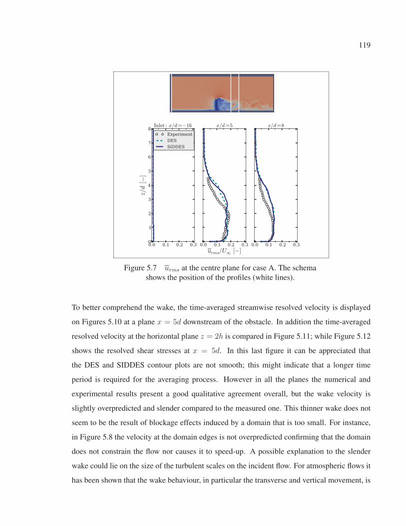
119

0.0 0.1 0.2 0.30

1

2

3

4

5

6

7

8

z/d

[−]

Inlet : x/d=−16

Experiment

DES

SIDDES

0.0 0.1 0.2 0.3

urms/U∞ [−]

x/d=5

0.0 0.1 0.2 0.3

x/d=8

Figure 5.7 urms at the centre plane for case A. The schema

shows the position of the profiles (white lines).

To better comprehend the wake, the time-averaged streamwise resolved velocity is displayed

on Figures 5.10 at a plane x = 5d downstream of the obstacle. In addition the time-averaged

resolved velocity at the horizontal plane z = 2h is compared in Figure 5.11; while Figure 5.12

shows the resolved shear stresses at x = 5d. In this last figure it can be appreciated that

the DES and SIDDES contour plots are not smooth; this might indicate that a longer time

period is required for the averaging process. However in all the planes the numerical and

experimental results present a good qualitative agreement overall, but the wake velocity is

slightly overpredicted and slender compared to the measured one. This thinner wake does not

seem to be the result of blockage effects induced by a domain that is too small. For instance,

in Figure 5.8 the velocity at the domain edges is not overpredicted confirming that the domain

does not constrain the flow nor causes it to speed-up. A possible explanation to the slender

wake could lie on the size of the turbulent scales on the incident flow. For atmospheric flows it

has been shown that the wake behaviour, in particular the transverse and vertical movement, is

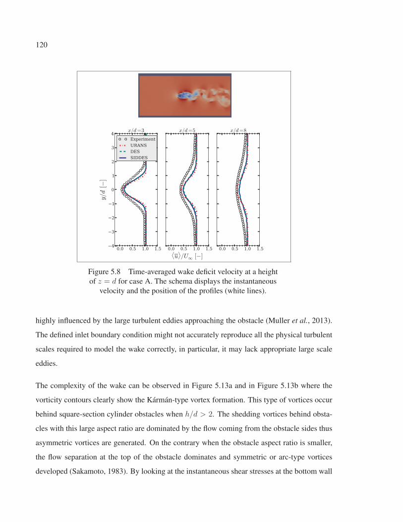
120

0.0 0.5 1.0 1.54

3

2

1

0

1

2

3

4

y/d[−

]

x/d=3

Experiment

URANS

DES

SIDDES

0.0 0.5 1.0 1.5⟨u⟩/U∞

[−]

x/d=5

0.0 0.5 1.0 1.5

x/d=8

Figure 5.8 Time-averaged wake deficit velocity at a height

of z = d for case A. The schema displays the instantaneous

velocity and the position of the profiles (white lines).

highly influenced by the large turbulent eddies approaching the obstacle (Muller et al., 2013).

The defined inlet boundary condition might not accurately reproduce all the physical turbulent

scales required to model the wake correctly, in particular, it may lack appropriate large scale

eddies.

The complexity of the wake can be observed in Figure 5.13a and in Figure 5.13b where the

vorticity contours clearly show the Kármán-type vortex formation. This type of vortices occur

behind square-section cylinder obstacles when h/d > 2. The shedding vortices behind obsta-

cles with this large aspect ratio are dominated by the flow coming from the obstacle sides thus

asymmetric vortices are generated. On the contrary when the obstacle aspect ratio is smaller,

the flow separation at the top of the obstacle dominates and symmetric or arc-type vortices

developed (Sakamoto, 1983). By looking at the instantaneous shear stresses at the bottom wall

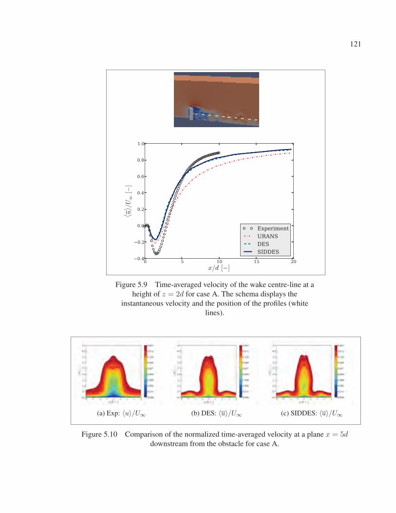
121

Figure 5.9 Time-averaged velocity of the wake centre-line at a

height of z = 2d for case A. The schema displays the

instantaneous velocity and the position of the profiles (white

lines).

(a) Exp: 〈u〉/U∞ (b) DES: 〈u〉/U∞ (c) SIDDES: 〈u〉/U∞

Figure 5.10 Comparison of the normalized time-averaged velocity at a plane x = 5ddownstream from the obstacle for case A.

122

(a) Exp: 〈u〉/U∞ (b) DES: 〈u〉/U∞ (c) SIDDES: 〈u〉/U∞

(d) Exp: 〈v〉/U∞ (e) DES: 〈v〉/U∞ (f) SIDDES: 〈v〉/U∞

(g) Exp: 〈w〉/U∞ (h) DES: 〈w〉/U∞ (i) SIDDES: 〈w〉/U∞

Figure 5.11 Upstream thin boundary layer case wake comparison at z = 2d. Case A.

in the hybrid simulations, the Kármán-type vortex can also be seen as display in Figure 5.14.

However, the time-averaged shear stresses give a different perception of the flow behaviour.

A visualization of the time-averaged velocity streamlines also sheds further insight of the wake

dynamics. In Figure 5.15, two recirculation bubbles are seen; one behind the obstacle and

another smaller one located in front at the obstacle’s base. A really interesting phenomena

is that the reverse flow region behind the obstacle does not reattached at the bottom wall.

However, shorter square-section cylinders (H/d << 3−4) do reattach at the wall (Wang et al.,

2006). This mentioned phenomena can be better perceived in Figure 5.16 where the time-

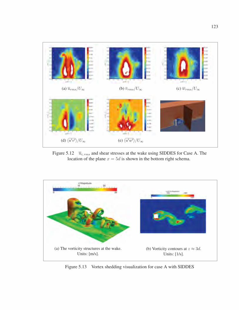
123

(a) urms/U∞ (b) vrms/U∞ (c) wrms/U∞

(d) 〈u′v′〉/U∞ (e) 〈u′w′〉/U∞

Figure 5.12 ui, rms and shear stresses at the wake using SIDDES for Case A. The

location of the plane x = 5d is shown in the bottom right schema.

(a) The vorticity structures at the wake.

Units: [m/s].

(b) Vorticity contours at z ≈ 3d.

Units: [1/s].

Figure 5.13 Vortex shedding visualization for case A with SIDDES

124

(a) Instantaneous (b) Time-averaged

Figure 5.14 Wall shear stresses at the bottom boundary for case A with SIDDES. The

colour bar represents the magnitude. Units: [m2/s2].

averaged velocity vectors clearly show upwash and a downwash region behind the obstacle.

Where the two regions collide a saddle point is present. The reverse flow regions can also be

distinguished by analyzing the wall shear stresses on the cylinder wall as in Figure 5.17. On

the front face, near the base of the obstacle a downwash flow (wall shear stress vectors pointing

upwards) confirms the existence of a recirculation bubble. Further from the cylinder base, the

flow just travels to the sides, around the obstacle. While on the back face, a region of upward

facing shear stress vectors is present at the base of the obstacle, and downward wall shear stress

vectors are located at the top. The change in flow direction is clearly seen.

Qualitatively, the resulted modelled wake displays the turbulent nature and vortex characteris-

tics described in the literature for this type of obstacles. Additionally, the results obtained by

the hybrid approaches are consistent with each other, and they show a fairly good agreement

with the wind-tunnel data. The computing time is somewhat smaller for the SIDDES cases

because of the slightly larger URANS regions. For case A, the SIDDES simulations required

only around 70% of the computing time needed for the DES simulations. However, the com-

puting time difference might not that relevant and the simpler DES could just be sufficient for

a case where the boundary layer is of the order of the grid spacing (streamwise and spanwise).

The increased complexity of the SIDDES might not be necessary for thin boundary layer cases.

Nevertheless, the GIS phenomena might arise for certain meshes, and it is not well handled by

DES.

125

Figure 5.15 Time-averaged velocity streamlines visualization with SIDDES for case

A. Units: [m/s].

Figure 5.16 Time-averaged velocity vectors for case A at the centre plane coloured

by averaged spanwise vorticity on the SIDDES computation. Units of colour bar: [1/s].

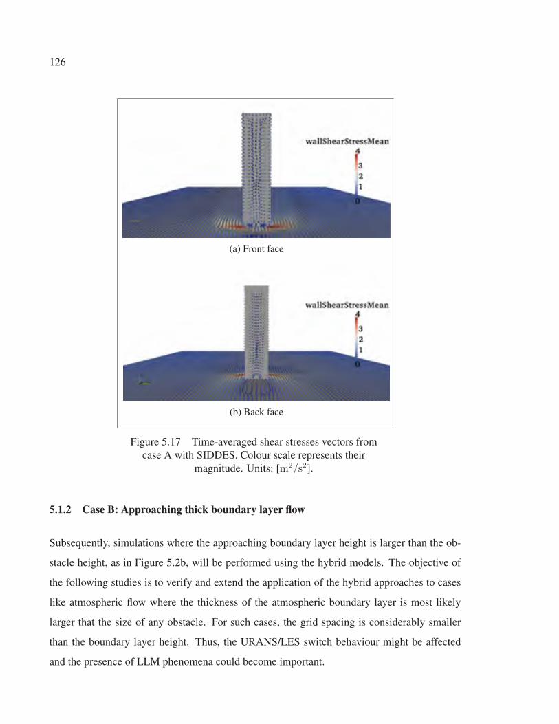
126

(a) Front face

(b) Back face

Figure 5.17 Time-averaged shear stresses vectors from

case A with SIDDES. Colour scale represents their

magnitude. Units: [m2/s2].

5.1.2 Case B: Approaching thick boundary layer flow

Subsequently, simulations where the approaching boundary layer height is larger than the ob-

stacle height, as in Figure 5.2b, will be performed using the hybrid models. The objective of

the following studies is to verify and extend the application of the hybrid approaches to cases

like atmospheric flow where the thickness of the atmospheric boundary layer is most likely

larger that the size of any obstacle. For such cases, the grid spacing is considerably smaller

than the boundary layer height. Thus, the URANS/LES switch behaviour might be affected

and the presence of LLM phenomena could become important.

127

Three different cases will be analyzed. Their characteristics are summarized in Table 5.1 and

they will be explained with more detail in this section. From the beginning, it is worth men-

tioning that case B1 and B2 do not represent a entirely valid nor physical test case. This will

become more apparent in the following paragraphs. However, it was deem important to show

these results in order to do a smooth transition between case A and B3.

Table 5.1 Square-section cylinder cases

A B1 B2 B3approaching BL: thin thick thick thick

inlet: imposed imposed imposed mappedprofiles profiles profiles precursor

outlet: zero-gradient zero-gradient zero-gradient zero-gradient

spanwise: periodic periodic periodic periodic

top: stress-free stress-free stress-free stress-free

solid walls: no-slip + no-slip + no-slip + no-slip +

rough ext. rough ext. rough ext. rough ext.

model constants: aerodynamic aerodynamic atmospheric atmospheric

5.1.2.1 Case B1: Imposed inlet profiles

The domain size, mesh resolution and boundary conditions are defined as in the previous

case A. The only difference is the profile defined at the inlet which in this case consist of

the sum of a mean logarithmic profile and time-correlated random fluctuations. The nominal

friction velocity was kept the same as in the previous case to keep the same mesh (since z+1

depends on u∗). This yields a utop = 19.6 m/s. The empty domain simulation results given

in Figure 5.18 show the resolved velocity and the resolved turbulence intensity profiles. The

plots for this case are still normalized by U∞ = 15 m/s for easier comparison. Surprisingly, the

LLM is not present in this case as it was expected. Further comments will be given about this

issue on Section 5.1.2.3. The resolved turbulence intensity is similar to case A.

The URANS/LES regions in the square-section cylinder approached by a thick boundary layer

flow simulations (case B1) are really similar to the previous case as it can be seen in Fig-

128

0.0 0.2 0.4 0.6 0.8 1.0 1.2 1.4⟨u⟩/U∞

[−]

0

2

4

6

8

10

12

z/d[−

]

x/d=0

DES

SIDDES

Log-law


0.00 0.050.0

0.5

1.0

1.5

2.0

2.5

z/d[−

]

x/d=Inlet

0.00 0.05

x/d=−7.87

0.00 0.05

urms/U∞ [−]

x/d=0.0

0.00 0.05

x/d=7.87

0.00 0.05

x/d=15.75

DES

SIDDES


Figure 5.18 Empty domain profiles for the thick boundary layer case (B1).

ure 5.19. Correspondingly, Figure 5.20 and Figure 5.21 display the velocity wake deficit and

the velocity downstream of the obstacle respectively. Notably, all the plots show that the DES

and SIDDES results are almost identical. This result was not at all expected for the fully im-

mersed obstacle case and seems to contradict the claim that thick boundary layer cases require

SIDDES to correct for the LLM.

15 10 5 0 5 10 15

x/d [−]

2

4

6

8

10

z/d

[−]

0.0

0.2

0.4

0.6

0.8

1.0

Regions

Figure 5.19 Case B1 instantaneous regions

using SIDDES. A pure LES region is identified

as 1 and a pure URANS as 0.

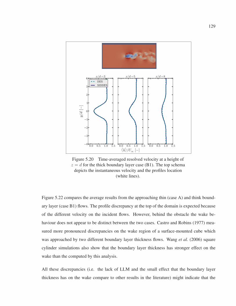
129

0.0 0.5 1.0 1.54

3

2

1

0

1

2

3

4

y/d[−

]

x/d=3

DES

SIDDES

0.0 0.5 1.0 1.5⟨u⟩/U∞

[−]

x/d=5

0.0 0.5 1.0 1.5

x/d=8

Figure 5.20 Time-averaged resolved velocity at a height of

z = d for the thick boundary layer case (B1). The top schema

depicts the instantaneous velocity and the profiles location

(white lines).

Figure 5.22 compares the average results from the approaching thin (case A) and think bound-

ary layer (case B1) flows. The profile discrepancy at the top of the domain is expected because

of the different velocity on the incident flows. However, behind the obstacle the wake be-

haviour does not appear to be distinct between the two cases. Castro and Robins (1977) mea-

sured more pronounced discrepancies on the wake region of a surface-mounted cube which

was approached by two different boundary layer thickness flows. Wang et al. (2006) square

cylinder simulations also show that the boundary layer thickness has stronger effect on the

wake than the computed by this analysis.

All these discrepancies (i.e. the lack of LLM and the small effect that the boundary layer

thickness has on the wake compare to other results in the literature) might indicate that the

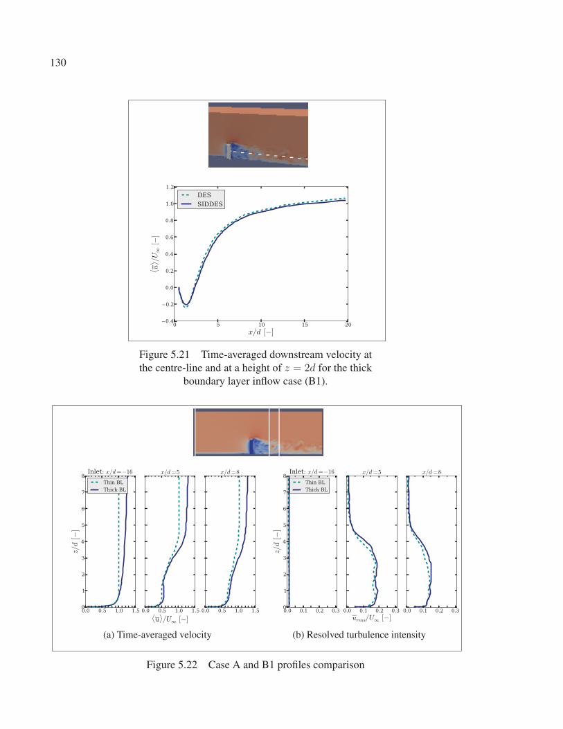
130

0 5 10 15 20

x/d [−]

0.4

0.2

0.0

0.2

0.4

0.6

0.8

1.0

1.2

⟨ u⟩ /U∞

[−]

DES

SIDDES

Figure 5.21 Time-averaged downstream velocity at

the centre-line and at a height of z = 2d for the thick

boundary layer inflow case (B1).

0.0 0.5 1.0 1.50

1

2

3

4

5

6

7

8

z/d[−

]

Inlet: x/d=−16

Thin BL

Thick BL

0.0 0.5 1.0 1.5⟨u⟩/U∞

[−]

x/d=5

0.0 0.5 1.0 1.5

x/d=8

(a) Time-averaged velocity

0.0 0.1 0.2 0.30

1

2

3

4

5

6

7

8

z/d[−

]

Inlet: x/d=−16

Thin BL

Thick BL

0.0 0.1 0.2 0.3

urms/U∞ [−]

x/d=5

0.0 0.1 0.2 0.3

x/d=8


Figure 5.22 Case A and B1 profiles comparison

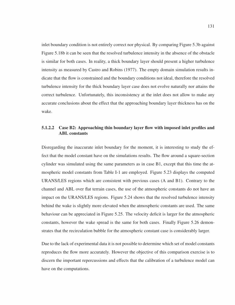
131

inlet boundary condition is not entirely correct nor physical. By comparing Figure 5.3b against

Figure 5.18b it can be seen that the resolved turbulence intensity in the absence of the obstacle

is similar for both cases. In reality, a thick boundary layer should present a higher turbulence

intensity as measured by Castro and Robins (1977). The empty domain simulation results in-

dicate that the flow is constrained and the boundary conditions not ideal, therefore the resolved

turbulence intensity for the thick boundary layer case does not evolve naturally nor attains the

correct turbulence. Unfortunately, this inconsistency at the inlet does not allow to make any

accurate conclusions about the effect that the approaching boundary layer thickness has on the

wake.

5.1.2.2 Case B2: Approaching thin boundary layer flow with imposed inlet profiles andABL constants

Disregarding the inaccurate inlet boundary for the moment, it is interesting to study the ef-

fect that the model constant have on the simulations results. The flow around a square-section

cylinder was simulated using the same parameters as in case B1, except that this time the at-

mospheric model constants from Table I-1 are employed. Figure 5.23 displays the computed

URANS/LES regions which are consistent with previous cases (A and B1). Contrary to the

channel and ABL over flat terrain cases, the use of the atmospheric constants do not have an

impact on the URANS/LES regions. Figure 5.24 shows that the resolved turbulence intensity

behind the wake is slightly more elevated when the atmospheric constants are used. The same

behaviour can be appreciated in Figure 5.25. The velocity deficit is larger for the atmospheric

constants, however the wake spread is the same for both cases. Finally Figure 5.26 demon-

strates that the recirculation bubble for the atmospheric constant case is considerably larger.

Due to the lack of experimental data it is not possible to determine which set of model constants

reproduces the flow more accurately. However the objective of this comparison exercise is to

discern the important repercussions and effects that the calibration of a turbulence model can

have on the computations.

132

15 10 5 0 5 10 15

x/d [−]

2

4

6

8

10

z/d

[−]

0.0

0.2

0.4

0.6

0.8

1.0

Regions

Figure 5.23 Time-averaged regions for the

SIDDES case B2. A pure LES region is identified as

1 and a pure URANS as 0.

0.0 0.5 1.0 1.50

1

2

3

4

5

6

7

8

z/d[−

]

Inlet: x/d=−16

0.0 0.5 1.0 1.5⟨u⟩/U∞

[−]

x/d=5

0.0 0.5 1.0 1.5

x/d=8

Aerodynamic constants

Atmospheric constants

(a) Time-averaged velocity

0.0 0.1 0.2 0.30

1

2

3

4

5

6

7

8

z/d[−

]

Inlet: x/d=−16

0.0 0.1 0.2 0.3

urms/U∞ [−]

x/d=5

0.0 0.1 0.2 0.3

x/d=8




Figure 5.24 Case B1 (aerodynamic constants) and B2 (atmospheric constants)

comparison using SIDDES.

133

0.0 0.5 1.0 1.54

3

2

1

0

1

2

3

4y/d[−

]

x/d=3

0.0 0.5 1.0 1.5⟨u⟩/U∞

[−]

x/d=5

0.0 0.5 1.0 1.5

x/d=8



Figure 5.25 Time-averaged resolved velocity at a height of

z = d for the thick boundary layer. Case B1 (aerodynamic

constants) and B2 (atmospheric constants) using SIDDES.

5.1.2.3 Case B3: Approaching thick boundary layer flow with mapped inlet from a pre-cursor simulation

A precursor simulation is employed to appropriately model a square-section cylinder sub-

merged in a ABL, in particular to correctly represent the inlet flow. As shown in Figure 5.27,

an empty domain with periodic boundary conditions and a thick boundary layer driven by a

constant large pressure gradient is computed first. A precursor simulation is basically a ABL

simulation over flat terrain. Within the precursor simulation the flow naturally develops the

turbulence structures and turbulence intensity. Once the simulations has reach statistical con-

vergence (∼ 20 − 30 flow-through times), the flow characteristics (i.e. u, k and ω) are saved

every time step at the outlet plane and used as a inlet boundary condition for a successor sim-

ulation. Contrary to the previous cases B1 and B2, a precursor simulation will yield an inlet

where all the flow properties (i.e. velocity, turbulence intensity, eddy size, etc.) are in agree-

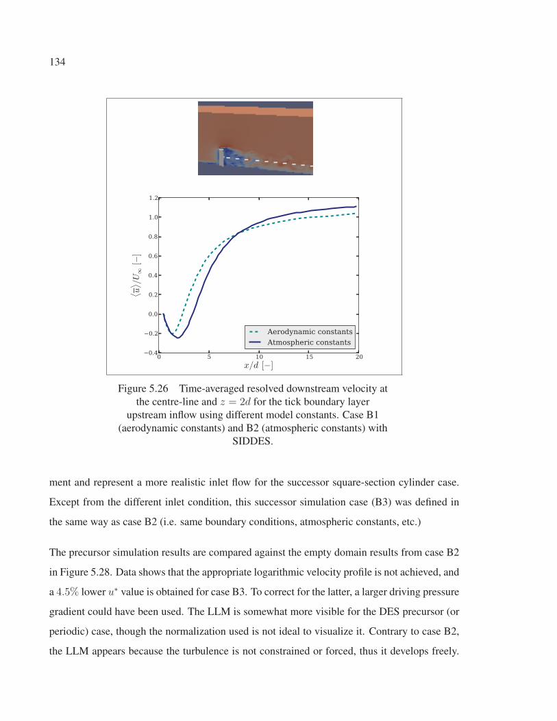
134

0 5 10 15 20

x/d [−]

0.4

0.2

0.0

0.2

0.4

0.6

0.8

1.0

1.2

⟨ u⟩ /U∞

[−]



Figure 5.26 Time-averaged resolved downstream velocity at

the centre-line and z = 2d for the tick boundary layer

upstream inflow using different model constants. Case B1

(aerodynamic constants) and B2 (atmospheric constants) with

SIDDES.

ment and represent a more realistic inlet flow for the successor square-section cylinder case.

Except from the different inlet condition, this successor simulation case (B3) was defined in

the same way as case B2 (i.e. same boundary conditions, atmospheric constants, etc.)

The precursor simulation results are compared against the empty domain results from case B2

in Figure 5.28. Data shows that the appropriate logarithmic velocity profile is not achieved, and

a 4.5% lower u∗ value is obtained for case B3. To correct for the latter, a larger driving pressure

gradient could have been used. The LLM is somewhat more visible for the DES precursor (or

periodic) case, though the normalization used is not ideal to visualize it. Contrary to case B2,

the LLM appears because the turbulence is not constrained or forced, thus it develops freely.

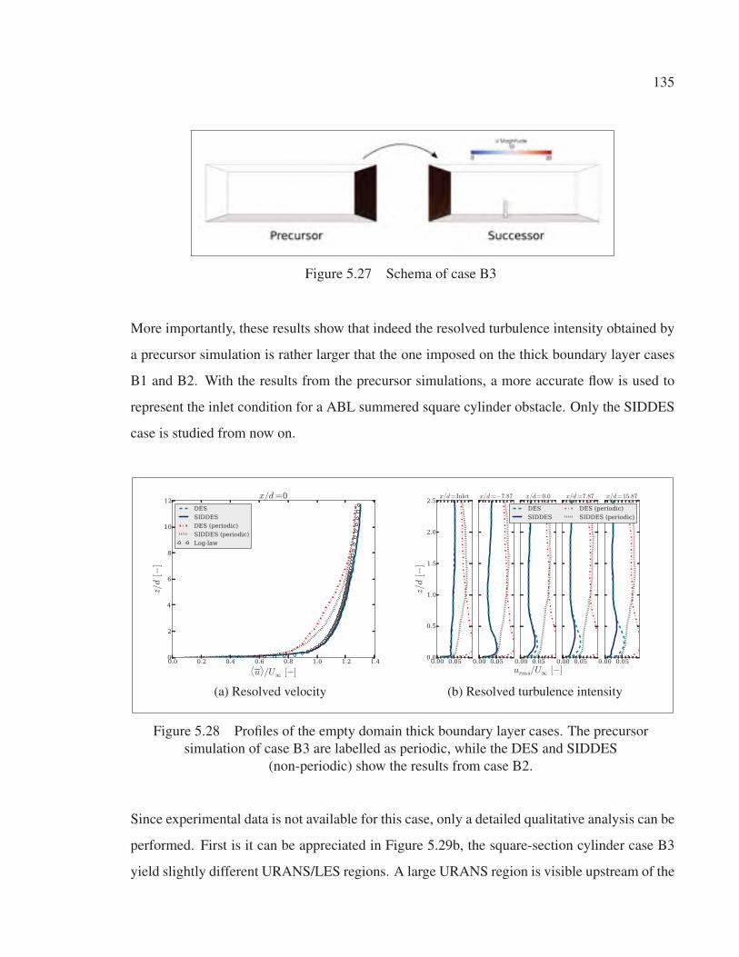
135

Figure 5.27 Schema of case B3

More importantly, these results show that indeed the resolved turbulence intensity obtained by

a precursor simulation is rather larger that the one imposed on the thick boundary layer cases

B1 and B2. With the results from the precursor simulations, a more accurate flow is used to

represent the inlet condition for a ABL summered square cylinder obstacle. Only the SIDDES

case is studied from now on.

(a) Resolved velocity (b) Resolved turbulence intensity

Figure 5.28 Profiles of the empty domain thick boundary layer cases. The precursor

simulation of case B3 are labelled as periodic, while the DES and SIDDES

(non-periodic) show the results from case B2.

Since experimental data is not available for this case, only a detailed qualitative analysis can be

performed. First is it can be appreciated in Figure 5.29b, the square-section cylinder case B3

yield slightly different URANS/LES regions. A large URANS region is visible upstream of the

136

obstacle because the precursor time-averaged URANS region (Figure 5.29a) is also large. The

URANS/LES regions obtained in this case are consistent with the flat terrain results. Next, the

normalized time-averaged velocity at plane downstream of the obstacle is seen in Figure 5.30.

It is evident that the wake is broader in the spanwise direction compared to the previous cases.

This could be linked to the larger eddy structures present at the inlet boundary condition. As

measured by Wang et al. (2006), two spanwise vortices are distinguished in Figure 5.30b at the

top of the obstacle. The vortices have opposite spanwise velocity components. In that same

figure, two base vortex is seen close to the wall. In a similar manner, two vortices are visible in

the vertical direction in Figure 5.30c. The ui, rms values and shear stresses at the same plane are

shown in Figure 5.31. These results are in quantitative agreement with the lateral distributions

measured by Wang et al. (2006). Also as it has been described in the literature (Wang et al.,

2006), the horseshoe vortex effect can be distinguished close to the wall at the side of the

obstacle in Figure 5.32. The streamline also show that most of the flow leaves the wake vortex

at a certain height approximately around z/h ∼ 2. The same phenomena is seen in case A,

thus the flow seems to escape the vortex at a much lower height (compare to Figure 5.15). This

is also an indication that in the thick approaching boundary layer case, the base vortex is larger

than in the thin boundary layer case as observed by Wang et al. (2006).

15 10 5 0 5 10 15

x/d [−]

2

4

6

8

10

z/d

[−]

0.0

0.2

0.4

0.6

0.8

1.0

Regions

(a) Precursor simulation

15 10 5 0 5 10 15

x/d [−]

2

4

6

8

10

z/d

[−]

0.0

0.2

0.4

0.6

0.8

1.0

Regions

(b) Successor simulation

Figure 5.29 Time-averaged URANS and LES regions for the SIDDES case B3. A

region of 1 represents a pure LES zone and 0 a pure URANS.

137

(a) 〈u〉/U∞ (b) 〈v〉/U∞ (c) 〈w〉/U∞

Figure 5.30 Time-averaged velocity at a plane x = 5d downstream from the obstacle

on case B3 using SIDDES.

(a) urms/U∞ (b) vrms/U∞ (c) wrms/U∞

(d) 〈u′v′〉/U∞ (e) 〈u′w′〉/U∞

Figure 5.31 ui, rms and shear stresses for case B3 at x = 5d using SIDDES.

The velocity vectors in the middle plane are shown in Figure 5.33. The upper and lower

vortices behind the obstacle are visible. As for the thin boundary layer case, the saddle point

exist and the recirculation bubble does not reattached at the wall. It has been demonstrated that

the saddle point height is dependent on the approaching boundary layer flow. As the boundary

layer thickness grows, the saddle point takes place further from the bottom wall and the upwash

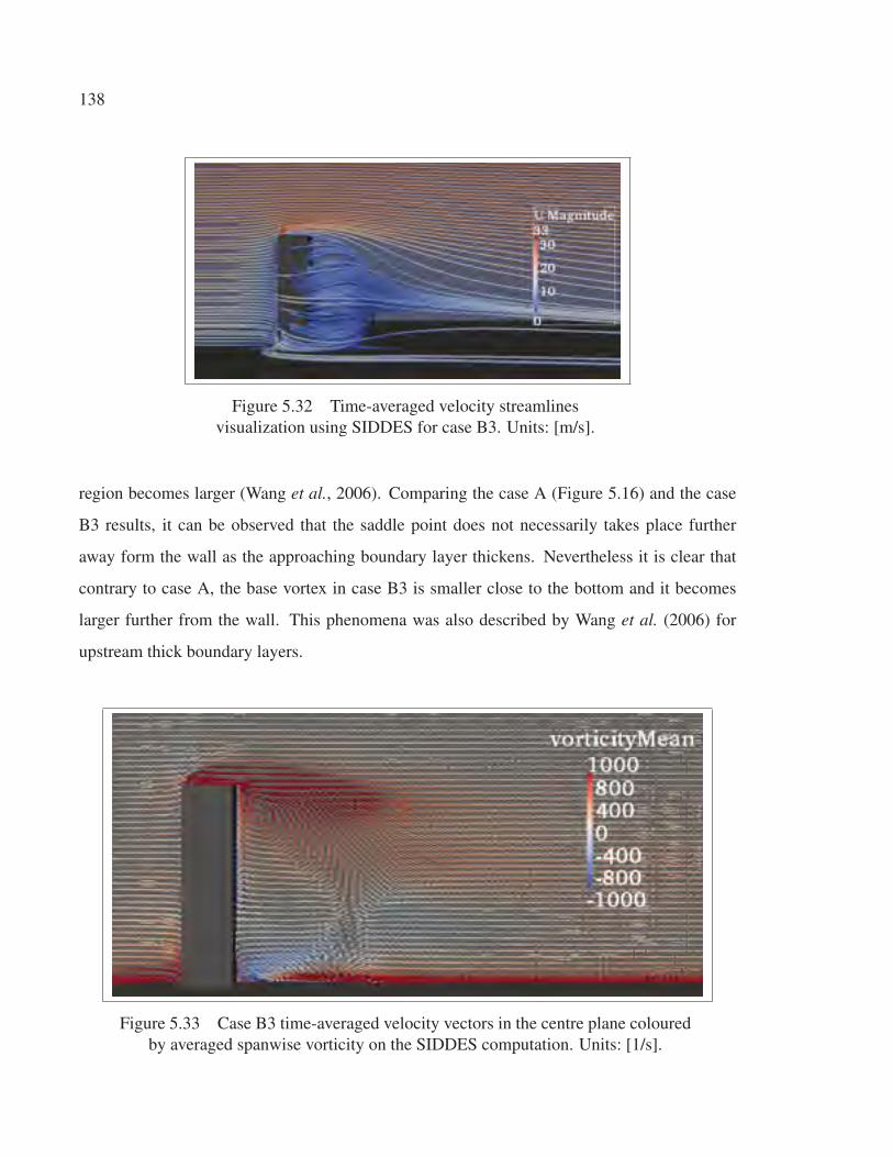
138

Figure 5.32 Time-averaged velocity streamlines

visualization using SIDDES for case B3. Units: [m/s].

region becomes larger (Wang et al., 2006). Comparing the case A (Figure 5.16) and the case

B3 results, it can be observed that the saddle point does not necessarily takes place further

away form the wall as the approaching boundary layer thickens. Nevertheless it is clear that

contrary to case A, the base vortex in case B3 is smaller close to the bottom and it becomes

larger further from the wall. This phenomena was also described by Wang et al. (2006) for

upstream thick boundary layers.

Figure 5.33 Case B3 time-averaged velocity vectors in the centre plane coloured

by averaged spanwise vorticity on the SIDDES computation. Units: [1/s].

139

In Figure 5.34a, the shear stress visualization at the obstacle’s front wall show that the flow

deviates sideways in most of the cylinder. Up to to a certain height and exactly at the centre

plane of the obstacle, the flow deviates downwards. Only a small part at the top of the obstacle

displays shear stresses indicating that the flow deviates upwards. This reproduced behaviour is

consistent with the shedding of a Kármán-type vortex (Sakamoto, 1983). Figure 5.34b shows

the presence of upward and downward flow. The recirculation bubble can also be seen in the

time-averaged wall shear stresses at the bottom wall displayed in Figure 5.35.

(a) Front face

(b) Back face

Figure 5.34 Time-averaged wall shear stresses vectors on the

cylinder for SIDDES case B3. Colour scale represents their

magnitude. Units: [m2/s2].

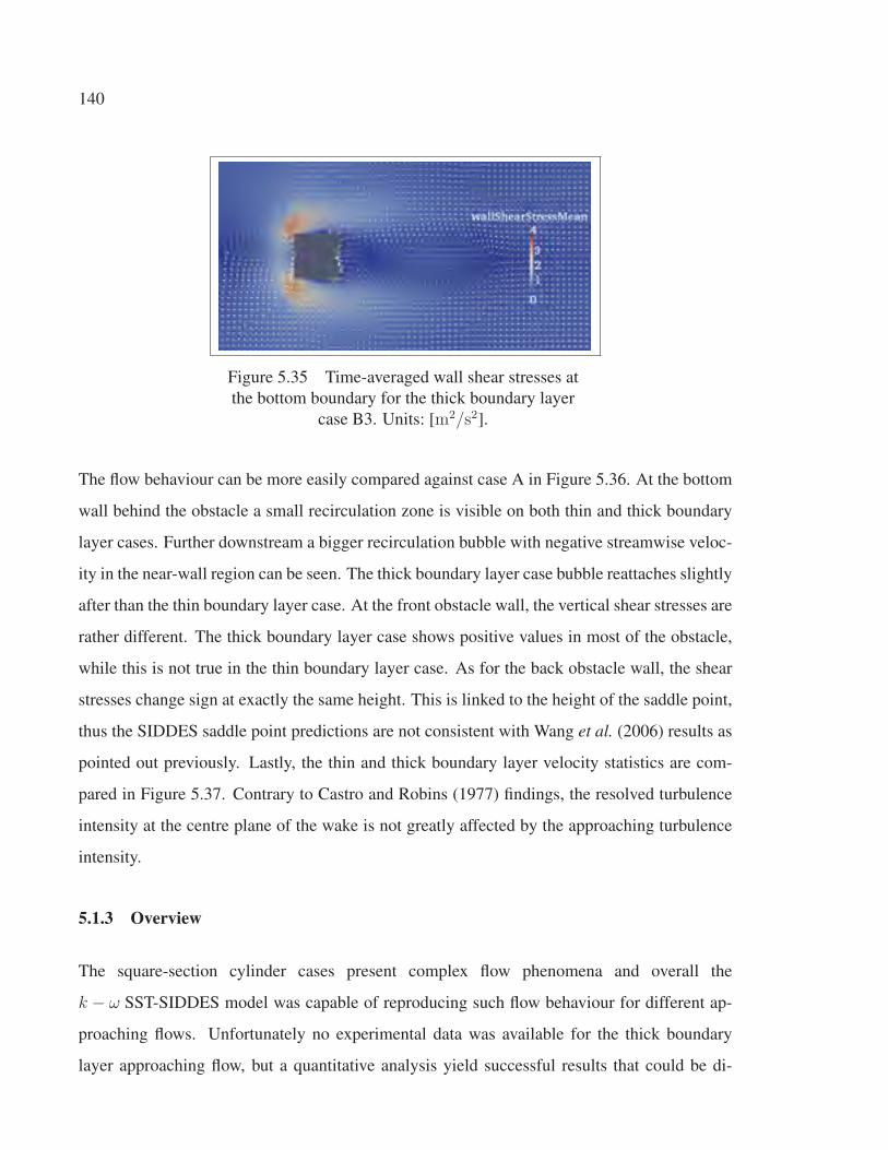
140

Figure 5.35 Time-averaged wall shear stresses at

the bottom boundary for the thick boundary layer

case B3. Units: [m2/s2].

The flow behaviour can be more easily compared against case A in Figure 5.36. At the bottom

wall behind the obstacle a small recirculation zone is visible on both thin and thick boundary

layer cases. Further downstream a bigger recirculation bubble with negative streamwise veloc-

ity in the near-wall region can be seen. The thick boundary layer case bubble reattaches slightly

after than the thin boundary layer case. At the front obstacle wall, the vertical shear stresses are

rather different. The thick boundary layer case shows positive values in most of the obstacle,

while this is not true in the thin boundary layer case. As for the back obstacle wall, the shear

stresses change sign at exactly the same height. This is linked to the height of the saddle point,

thus the SIDDES saddle point predictions are not consistent with Wang et al. (2006) results as

pointed out previously. Lastly, the thin and thick boundary layer velocity statistics are com-

pared in Figure 5.37. Contrary to Castro and Robins (1977) findings, the resolved turbulence

intensity at the centre plane of the wake is not greatly affected by the approaching turbulence

intensity.

5.1.3 Overview

The square-section cylinder cases present complex flow phenomena and overall the

k − ω SST-SIDDES model was capable of reproducing such flow behaviour for different ap-

proaching flows. Unfortunately no experimental data was available for the thick boundary

layer approaching flow, but a quantitative analysis yield successful results that could be di-

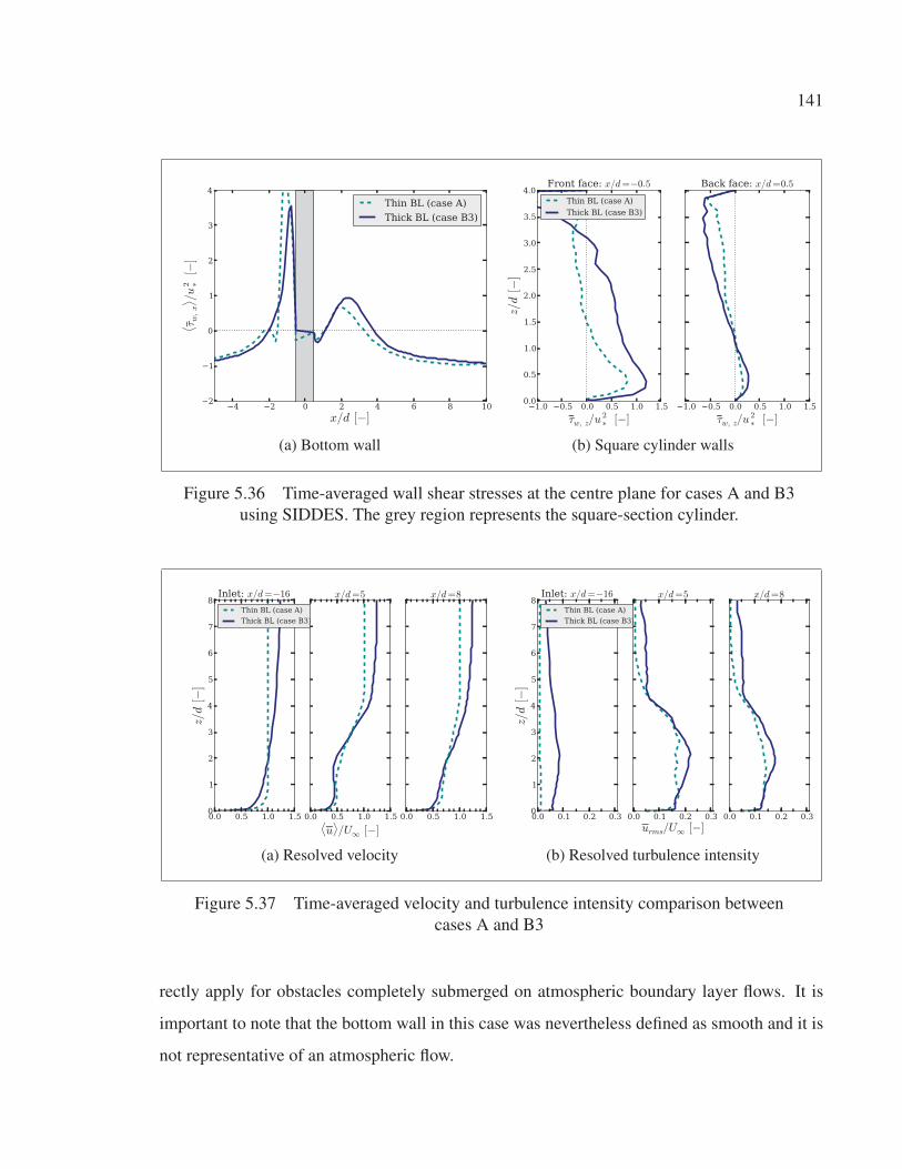
141

4 2 0 2 4 6 8 10

x/d [−]

2

1

0

1

2

3

4

⟨ τ w,x

⟩ /u

2 ∗[−

]Thin BL (case A)

Thick BL (case B3)

(a) Bottom wall

1.0 0.5 0.0 0.5 1.0 1.5

τw, z/u2∗

[−]

0.0

0.5

1.0

1.5

2.0

2.5

3.0

3.5

4.0

z/d[−

]

Front face: x/d=−0.5

Thin BL (case A)

Thick BL (case B3)

1.0 0.5 0.0 0.5 1.0 1.5

τw, z/u2∗

[−]

Back face: x/d=0.5

(b) Square cylinder walls

Figure 5.36 Time-averaged wall shear stresses at the centre plane for cases A and B3

using SIDDES. The grey region represents the square-section cylinder.

0.0 0.5 1.0 1.50

1

2

3

4

5

6

7

8

z/d[−

]

Inlet: x/d=−16

Thin BL (case A)

Thick BL (case B3)

0.0 0.5 1.0 1.5⟨u⟩/U∞

[−]

x/d=5

0.0 0.5 1.0 1.5

x/d=8


0.0 0.1 0.2 0.30

1

2

3

4

5

6

7

8

z/d[−

]

Inlet: x/d=−16

Thin BL (case A)

Thick BL (case B3)

0.0 0.1 0.2 0.3

urms/U∞ [−]

x/d=5

0.0 0.1 0.2 0.3

x/d=8


Figure 5.37 Time-averaged velocity and turbulence intensity comparison between

cases A and B3

rectly apply for obstacles completely submerged on atmospheric boundary layer flows. It is

important to note that the bottom wall in this case was nevertheless defined as smooth and it is

not representative of an atmospheric flow.

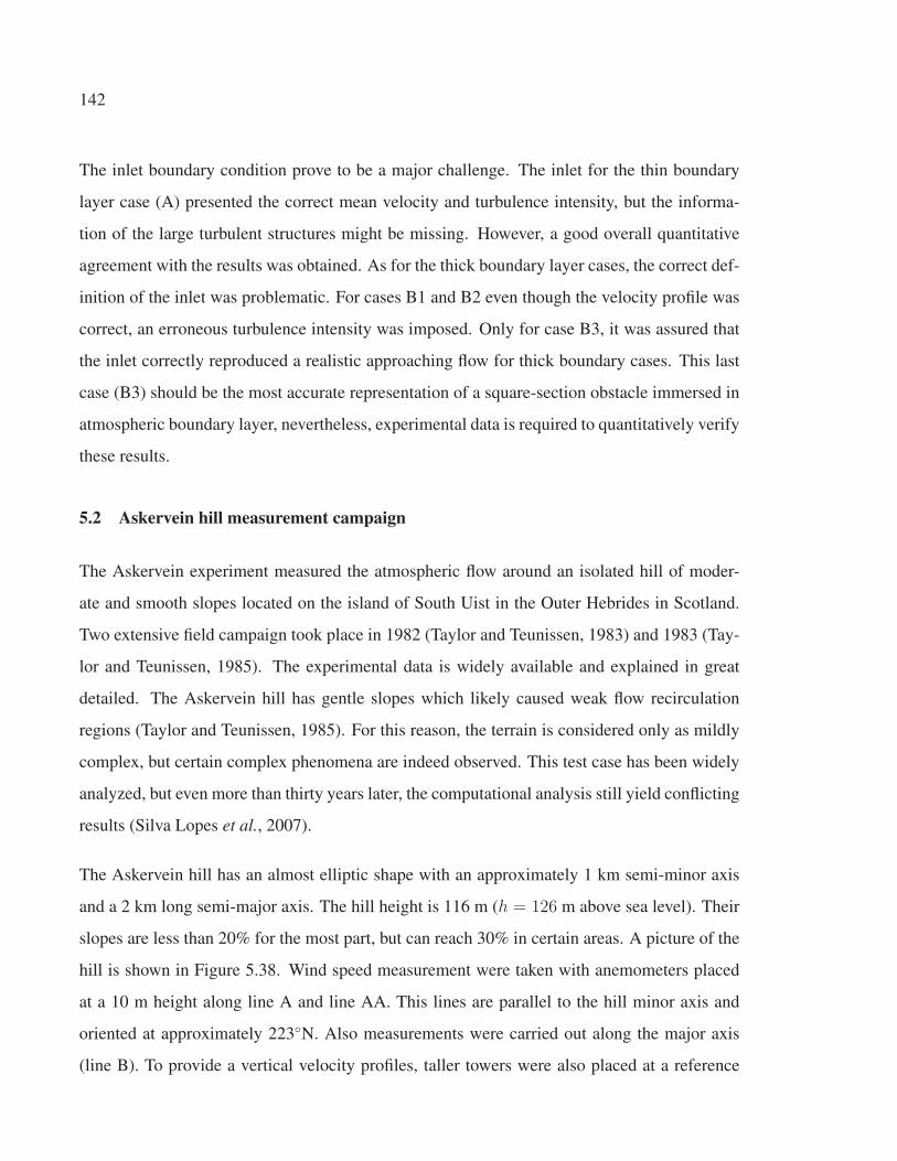
142

The inlet boundary condition prove to be a major challenge. The inlet for the thin boundary

layer case (A) presented the correct mean velocity and turbulence intensity, but the informa-

tion of the large turbulent structures might be missing. However, a good overall quantitative

agreement with the results was obtained. As for the thick boundary layer cases, the correct def-

inition of the inlet was problematic. For cases B1 and B2 even though the velocity profile was

correct, an erroneous turbulence intensity was imposed. Only for case B3, it was assured that

the inlet correctly reproduced a realistic approaching flow for thick boundary cases. This last

case (B3) should be the most accurate representation of a square-section obstacle immersed in

atmospheric boundary layer, nevertheless, experimental data is required to quantitatively verify

these results.

5.2 Askervein hill measurement campaign

The Askervein experiment measured the atmospheric flow around an isolated hill of moder-

ate and smooth slopes located on the island of South Uist in the Outer Hebrides in Scotland.

Two extensive field campaign took place in 1982 (Taylor and Teunissen, 1983) and 1983 (Tay-

lor and Teunissen, 1985). The experimental data is widely available and explained in great

detailed. The Askervein hill has gentle slopes which likely caused weak flow recirculation

regions (Taylor and Teunissen, 1985). For this reason, the terrain is considered only as mildly

complex, but certain complex phenomena are indeed observed. This test case has been widely

analyzed, but even more than thirty years later, the computational analysis still yield conflicting

results (Silva Lopes et al., 2007).

The Askervein hill has an almost elliptic shape with an approximately 1 km semi-minor axis

and a 2 km long semi-major axis. The hill height is 116 m (h = 126 m above sea level). Their

slopes are less than 20% for the most part, but can reach 30% in certain areas. A picture of the

hill is shown in Figure 5.38. Wind speed measurement were taken with anemometers placed

at a 10 m height along line A and line AA. This lines are parallel to the hill minor axis and

oriented at approximately 223◦N. Also measurements were carried out along the major axis

(line B). To provide a vertical velocity profiles, taller towers were also placed at a reference

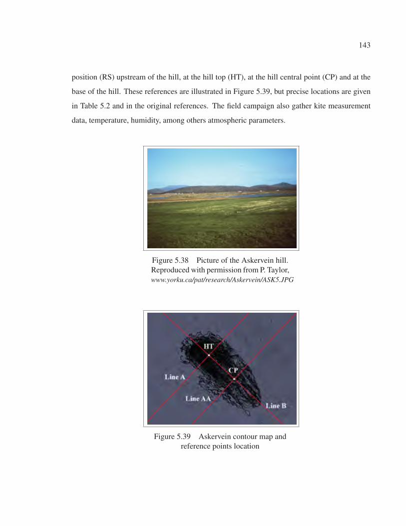
143

position (RS) upstream of the hill, at the hill top (HT), at the hill central point (CP) and at the

base of the hill. These references are illustrated in Figure 5.39, but precise locations are given

in Table 5.2 and in the original references. The field campaign also gather kite measurement

data, temperature, humidity, among others atmospheric parameters.

Figure 5.38 Picture of the Askervein hill.

Reproduced with permission from P. Taylor,

www.yorku.ca/pat/research/Askervein/ASK5.JPG

Figure 5.39 Askervein contour map and

reference points location

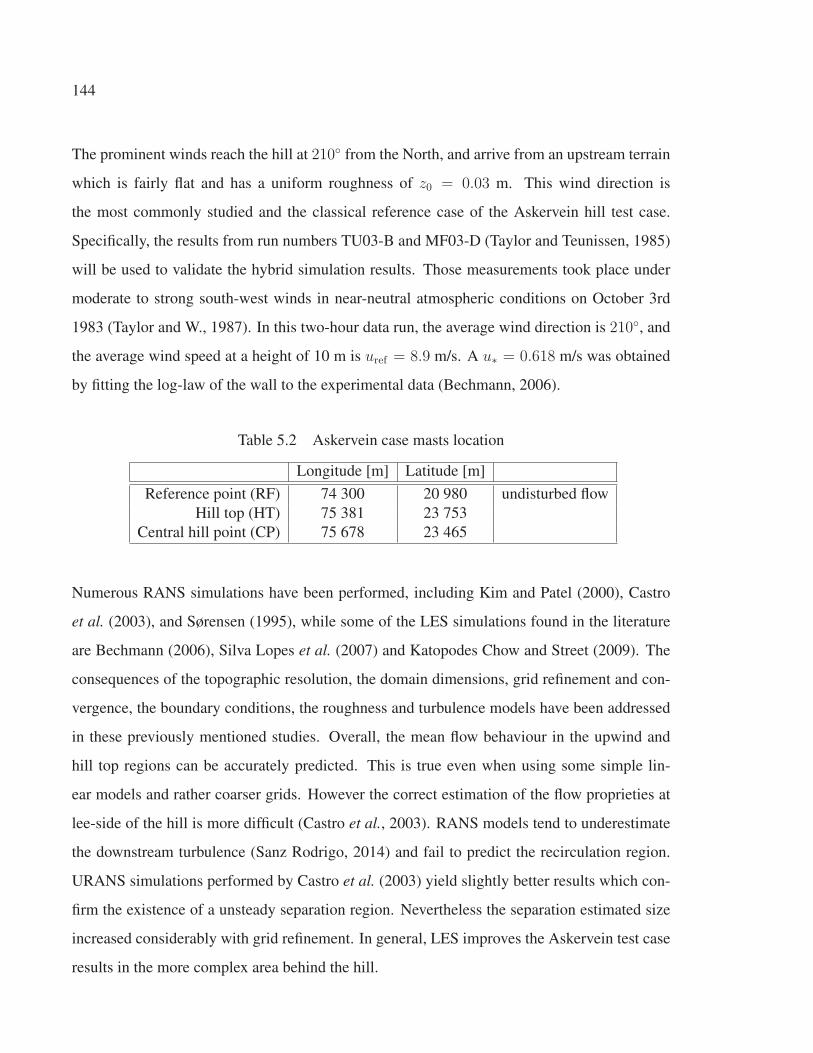
144

The prominent winds reach the hill at 210◦ from the North, and arrive from an upstream terrain

which is fairly flat and has a uniform roughness of z0 = 0.03 m. This wind direction is

the most commonly studied and the classical reference case of the Askervein hill test case.

Specifically, the results from run numbers TU03-B and MF03-D (Taylor and Teunissen, 1985)

will be used to validate the hybrid simulation results. Those measurements took place under

moderate to strong south-west winds in near-neutral atmospheric conditions on October 3rd

1983 (Taylor and W., 1987). In this two-hour data run, the average wind direction is 210◦, and

the average wind speed at a height of 10 m is uref = 8.9 m/s. A u∗ = 0.618 m/s was obtained

by fitting the log-law of the wall to the experimental data (Bechmann, 2006).

Table 5.2 Askervein case masts location

Longitude [m] Latitude [m]

Reference point (RF) 74 300 20 980 undisturbed flow

Hill top (HT) 75 381 23 753

Central hill point (CP) 75 678 23 465

Numerous RANS simulations have been performed, including Kim and Patel (2000), Castro

et al. (2003), and Sørensen (1995), while some of the LES simulations found in the literature

are Bechmann (2006), Silva Lopes et al. (2007) and Katopodes Chow and Street (2009). The

consequences of the topographic resolution, the domain dimensions, grid refinement and con-

vergence, the boundary conditions, the roughness and turbulence models have been addressed

in these previously mentioned studies. Overall, the mean flow behaviour in the upwind and

hill top regions can be accurately predicted. This is true even when using some simple lin-

ear models and rather coarser grids. However the correct estimation of the flow proprieties at

lee-side of the hill is more difficult (Castro et al., 2003). RANS models tend to underestimate

the downstream turbulence (Sanz Rodrigo, 2014) and fail to predict the recirculation region.

URANS simulations performed by Castro et al. (2003) yield slightly better results which con-

firm the existence of a unsteady separation region. Nevertheless the separation estimated size

increased considerably with grid refinement. In general, LES improves the Askervein test case

results in the more complex area behind the hill.

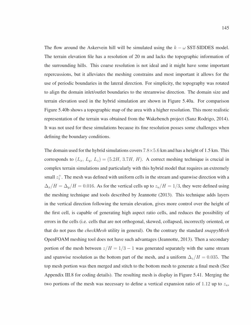
145

The flow around the Askervein hill will be simulated using the k − ω SST-SIDDES model.

The terrain elevation file has a resolution of 20 m and lacks the topographic information of

the surrounding hills. This coarse resolution is not ideal and it might have some important

repercussions, but it alleviates the meshing constrains and most important it allows for the

use of periodic boundaries in the lateral direction. For simplicity, the topography was rotated

to align the domain inlet/outlet boundaries to the streamwise direction. The domain size and

terrain elevation used in the hybrid simulation are shown in Figure 5.40a. For comparison

Figure 5.40b shows a topographic map of the area with a higher resolution. This more realistic

representation of the terrain was obtained from the Wakebench project (Sanz Rodrigo, 2014).

It was not used for these simulations because its fine resolution posses some challenges when

defining the boundary conditions.

The domain used for the hybrid simulations covers 7.8×5.6 km and has a height of 1.5 km. This

corresponds to (Lx, Ly, Lz) = (5.2H, 3.7H, H). A correct meshing technique is crucial in

complex terrain simulations and particularly with this hybrid model that requires an extremely

small z+1 . The mesh was defined with uniform cells in the stream and spanwise direction with a

Δx/H = Δy/H = 0.016. As for the vertical cells up to zu/H = 1/3, they were defined using

the meshing technique and tools described by Jeannotte (2013). This technique adds layers

in the vertical direction following the terrain elevation, gives more control over the height of

the first cell, is capable of generating high aspect ratio cells, and reduces the possibility of

errors in the cells (i.e. cells that are not orthogonal, skewed, collapsed, incorrectly oriented, or

that do not pass the checkMesh utility in general). On the contrary the standard snappyMesh

OpenFOAM meshing tool does not have such advantages (Jeannotte, 2013). Then a secondary

portion of the mesh between z/H = 1/3− 1 was generated separately with the same stream

and spanwise resolution as the bottom part of the mesh, and a uniform Δz/H = 0.035. The

top mesh portion was then merged and stitch to the bottom mesh to generate a final mesh (See

Appendix III.8 for coding details). The resulting mesh is display in Figure 5.41. Merging the

two portions of the mesh was necessary to define a vertical expansion ratio of 1.12 up to zu,

146

(a) Domain and terrain representation used in the hybrid

simulations

(b) A more realistic terrain. Not used in the hybrid simulations.

Figure 5.40 Top view of the Askervein hill

and also to avoid extremely elongated cells in the top two thirds of the domain which are not

recommended in LES regions.

Two different meshes are analyzed. They both have the same number of cells in the stream and

spanwise, but different z1. The specific grid parameters are given in Table 5.3. Unfortunately

even with the mentioned meshing technique, the required z+1 ∼ 1.0 could not be attained with-

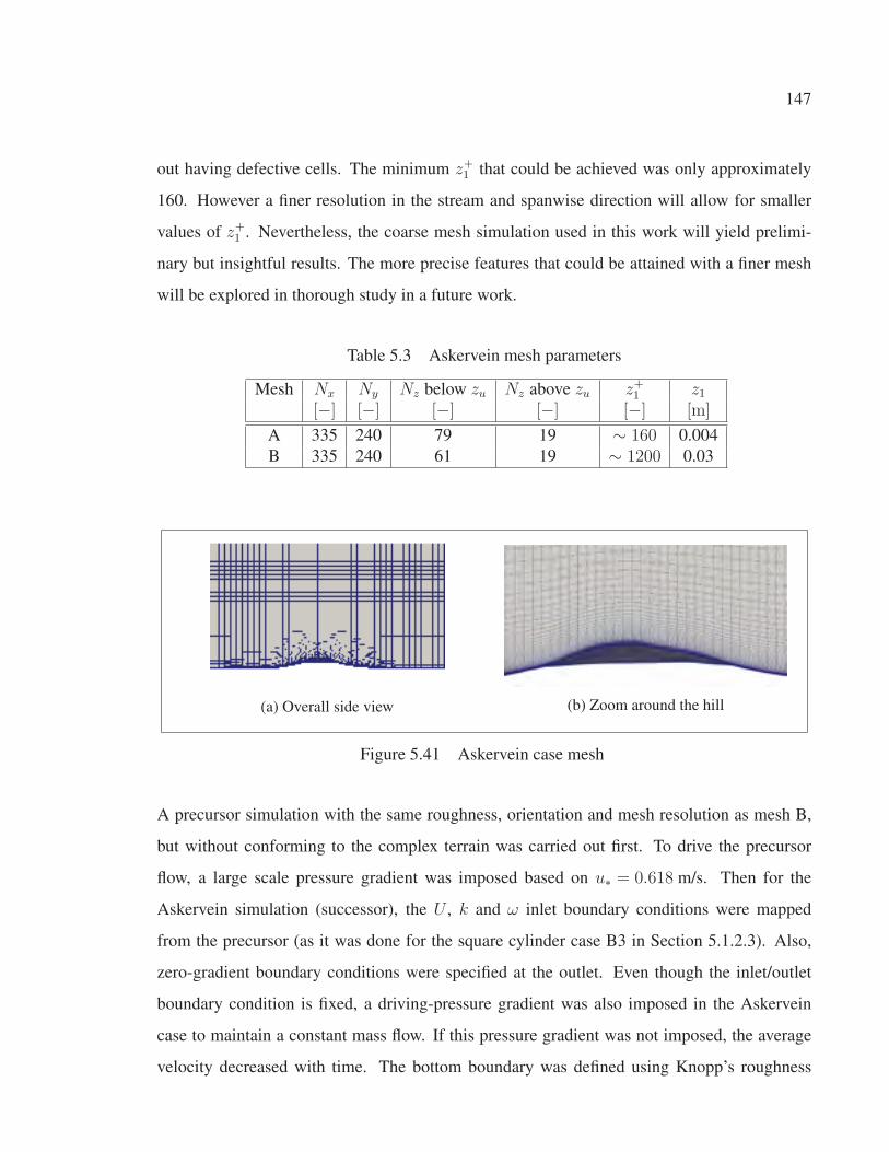
147

out having defective cells. The minimum z+1 that could be achieved was only approximately

160. However a finer resolution in the stream and spanwise direction will allow for smaller

values of z+1 . Nevertheless, the coarse mesh simulation used in this work will yield prelimi-

nary but insightful results. The more precise features that could be attained with a finer mesh

will be explored in thorough study in a future work.

Table 5.3 Askervein mesh parameters

Mesh Nx Ny Nz below zu Nz above zu z+1 z1[−] [−] [−] [−] [−] [m]

A 335 240 79 19 ∼ 160 0.004

B 335 240 61 19 ∼ 1200 0.03

(a) Overall side view (b) Zoom around the hill

Figure 5.41 Askervein case mesh

A precursor simulation with the same roughness, orientation and mesh resolution as mesh B,

but without conforming to the complex terrain was carried out first. To drive the precursor

flow, a large scale pressure gradient was imposed based on u∗ = 0.618 m/s. Then for the

Askervein simulation (successor), the U , k and ω inlet boundary conditions were mapped

from the precursor (as it was done for the square cylinder case B3 in Section 5.1.2.3). Also,

zero-gradient boundary conditions were specified at the outlet. Even though the inlet/outlet

boundary condition is fixed, a driving-pressure gradient was also imposed in the Askervein

case to maintain a constant mass flow. If this pressure gradient was not imposed, the average

velocity decreased with time. The bottom boundary was defined using Knopp’s roughness

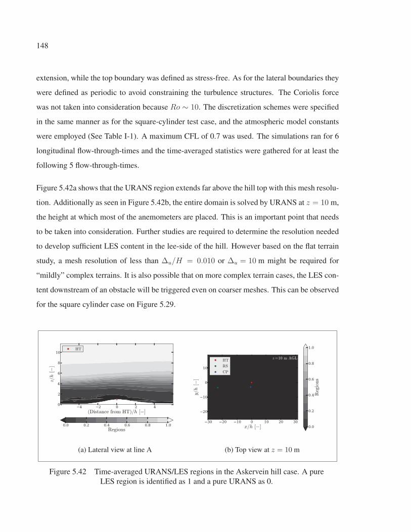
148

extension, while the top boundary was defined as stress-free. As for the lateral boundaries they

were defined as periodic to avoid constraining the turbulence structures. The Coriolis force

was not taken into consideration because Ro ∼ 10. The discretization schemes were specified

in the same manner as for the square-cylinder test case, and the atmospheric model constants

were employed (See Table I-1). A maximum CFL of 0.7 was used. The simulations ran for 6

longitudinal flow-through-times and the time-averaged statistics were gathered for at least the

following 5 flow-through-times.

Figure 5.42a shows that the URANS region extends far above the hill top with this mesh resolu-

tion. Additionally as seen in Figure 5.42b, the entire domain is solved by URANS at z = 10 m,

the height at which most of the anemometers are placed. This is an important point that needs

to be taken into consideration. Further studies are required to determine the resolution needed

to develop sufficient LES content in the lee-side of the hill. However based on the flat terrain

study, a mesh resolution of less than Δu/H = 0.010 or Δu = 10 m might be required for

“mildly” complex terrains. It is also possible that on more complex terrain cases, the LES con-

tent downstream of an obstacle will be triggered even on coarser meshes. This can be observed

for the square cylinder case on Figure 5.29.

4 2 0 2 4

(Distance from HT)/h [−]

0

2

4

6

8

10

z/h[−

]

HT

0.0 0.2 0.4 0.6 0.8 1.0

Regions

(a) Lateral view at line A

30 20 10 0 10 20 30

x/h [−]

20

10

0

10

y/h[−]

z=10 m AGLHT

RS

CP

0.0

0.2

0.4

0.6

0.8

1.0

Regions

(b) Top view at z = 10 m

Figure 5.42 Time-averaged URANS/LES regions in the Askervein hill case. A pure

LES region is identified as 1 and a pure URANS as 0.

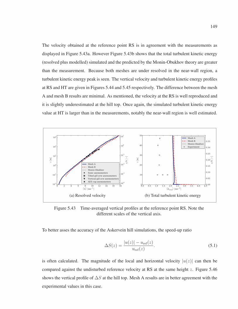
149

The velocity obtained at the reference point RS is in agreement with the measurements as

displayed in Figure 5.43a. However Figure 5.43b shows that the total turbulent kinetic energy

(resolved plus modelled) simulated and the predicted by the Monin-Obukhov theory are greater

than the measurement. Because both meshes are under resolved in the near-wall region, a

turbulent kinetic energy peak is seen. The vertical velocity and turbulent kinetic energy profiles

at RS and HT are given in Figures 5.44 and 5.45 respectively. The difference between the mesh

A and mesh B results are minimal. As mentioned, the velocity at the RS is well reproduced and

it is slightly underestimated at the hill top. Once again, the simulated turbulent kinetic energy

value at HT is larger than in the measurements, notably the near-wall region is well estimated.

10-4

10-3

10-2

10-1

100

101

z/h

[−]

10-2

10-1

100

101

102

103

z[m

]

0 2 4 6 8 10 12 14 16 18⟨u⟩[ms−1 ]

Mesh A

Mesh B

Monin-Obukhov

Sonic anemometers

Tilted gill uvw anemometers

Vertical gill uvw anemometers

AES cup anemometers


0.00

0.05

0.10

0.15

0.20

0.25

0.30

0.35

z/h

[−]

0

10

20

30

40

50z[m

]

0.0 0.5 1.0 1.5 2.0 2.5 3.0 3.5 4.0 4.5⟨ktotal

⟩[ms−2 ]

Mesh A

Mesh B

Monin-Obukhov

Experiment

(b) Total turbulent kinetic energy

Figure 5.43 Time-averaged vertical profiles at the reference point RS. Note the

different scales of the vertical axis.

To better asses the accuracy of the Askervein hill simulations, the speed-up ratio

ΔS(z) =|u(z)| − uref(z)

uref(z). (5.1)

is often calculated. The magnitude of the local and horizontal velocity |u(z)| can then be

compared against the undisturbed reference velocity at RS at the same height z. Figure 5.46

shows the vertical profile of ΔS at the hill top. Mesh A results are in better agreement with the

experimental values in this case.

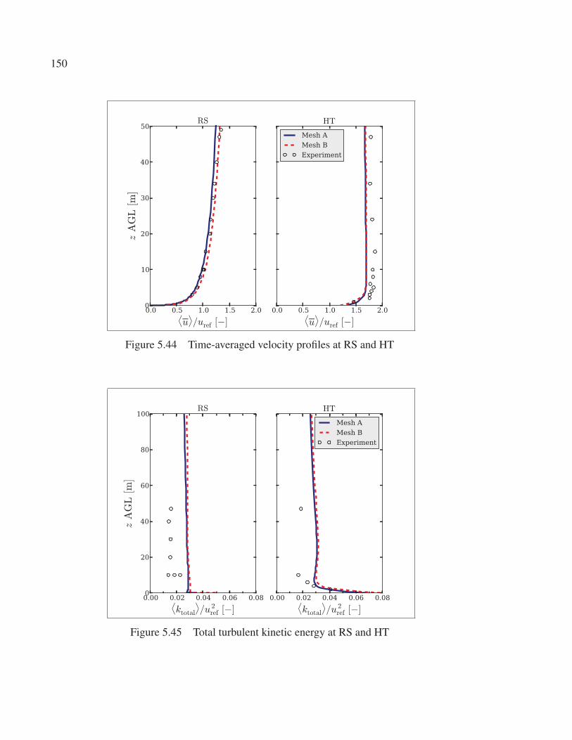
150

0.0 0.5 1.0 1.5 2.0⟨u⟩/uref [−]

0

10

20

30

40

50zAGL[m]

RS

0.0 0.5 1.0 1.5 2.0⟨u⟩/uref [−]

HT

Mesh A

Mesh B

Experiment

Figure 5.44 Time-averaged velocity profiles at RS and HT

0.00 0.02 0.04 0.06 0.08⟨ktotal

⟩/u 2

ref [−]

0

20

40

60

80

100

zAGL[m

]

RS

0.00 0.02 0.04 0.06 0.08⟨ktotal

⟩/u 2

ref [−]

HT

Mesh A

Mesh B

Experiment

Figure 5.45 Total turbulent kinetic energy at RS and HT

151

0.00

0.05

0.10

0.15

0.20

0.25

0.30

0.35

z/h[−]

0

10

20

30

40

50

zAGL[m]

0.0 0.5 1.0 1.5 2.0

ΔS [−]

Mesh A

Mesh B

Experiment

Figure 5.46 Vertical speed-up ratio at HT

Across the hill along line A and AA, the speed-up ratio at z = 10 m is rather accurately re-

produced in the upstream region. This can be noticed in Figure 5.47. Nevertheless, the sharp

deceleration in the lee-side of the hill along line A is not correctly predicted by the hybrid

model. Downstream, the ΔS value can indicate the existence of a possible recirculation re-

gion (Katopodes Chow and Street, 2009). As for the normalized turbulent kinetic energy along

line A and AA in Figure 5.48, the hybrid model results are not consistent with the experimental

data. However in general, RANS models and even coarse mesh LES results (Silva Lopes et al.,

2007) tend to under estimate the turbulence downstream of the hill.

Finally, Figure 5.49a gives a global perception of the mean velocity field at a height of 10 m,

while the instantaneous velocity field near the hill is shown in Figure 5.49b. These simulations

do not indicate the presence of a recirculation region in the lee-side of the hill.

5.2.1 Overview

Even with a simplified terrain representation and a coarse topographic resolution, the neutral

atmospheric flow around the Askervein hill was properly estimated by the k − ω SST-SIDDES

hybrid model. Due to the coarse mesh refinement used, most of the results shown come from

152

1000 500 0 500 1000


0.8

0.6

0.4

0.2

0.0

0.2

0.4

0.6

0.8

1.0

ΔS[−

]

Mesh A

Mesh B

Experiment

(a) Along line A

1000 500 0 500 1000

(Distance from CP)/h [−]

0.8

0.6

0.4

0.2

0.0

0.2

0.4

0.6

0.8

1.0

ΔS[−

]

Mesh A

Mesh B

Experiment

(b) Along line AA

Figure 5.47 Speed-up across the Askervein hill at z = 10 m

1000 500 0 500 1000


0.01

0.02

0.03

0.04

0.05

0.06

0.07

⟨ ktotal⟩ /

u2 ref[−

]

Mesh A

Mesh B

Experiment

(a) Along line A

1000 500 0 500 1000 1500

(Distance from CP)/h [−]

0.01

0.02

0.03

0.04

0.05

0.06

0.07

⟨ kto

tal⟩ /

u2 ref[−

]

Mesh A

Mesh B

Experiment

(b) Along line AA

Figure 5.48 Turbulent kinetic energy across the Askervein hill at z = 10 m

URANS regions in the simulation. As it is often seen on RANS simulations, the hybrid results

reproduce accurately the mean velocity field, but encounter difficulties to correctly estimate

unsteady phenomena and turbulence statistics (i.e the turbulent kinetic energy and the recircu-

lation region).

153

30 20 10 0 10 20 30

x/h [−]

20

10

0

10

y/h[−]

z=10 m AGLHT

RS

CP

0.4

0.6

0.7

0.8

1.0

1.1

1.2

1.4

1.5

1.6

|⟨ u

⟩ |/uref[−]

(a) Magnitude of the mean horizontal velocity

3 2 1 0 1 2 3 4

x/h [−]

4

3

2

1

0

1

2

3

y/h[−]

z=10 m AGLHT

RS

CP

0.4

0.6

0.8

1.0

1.1

1.3

1.5

1.7

u/uref[−]

(b) Instantaneous streamwise velocity

Figure 5.49 Mesh A velocity field at z = 10 m

154

The hybrid model results could potentially be improved with a finer mesh. First, smaller cells

will push the LES regions closer to the ground, possibly allowing the prediction of unsteady

behaviour in the lee-side of the hill. Secondly, having a finer mesh will reduce the aspect ratio

of the near-wall cells and alleviate the meshing constrains. Therefore, having smaller cells in

the stream and spanwise direction will allow smaller values z1 without introducing errors in

the mesh and the required z+1 will be more easily attainable.

These results do not appear to indicate that having a large z+1 (without a wall function) could

lead to any discrepancies or unphysical behaviour in the simulations. As shown on the flat

terrain cases in Section 4.2, it might not be necessary to have z+1 ∼ 1.0 for atmospheric flow

simulations if its consequences are understood (i.e. peak in the turbulent kinetic energy profile

and the inaccurate estimation of u∗). But to firmly corroborate that statement finer mesh test

cases need to be analyzed.

On the other hand, Castro et al. (2003) considered that the inaccuracies in their Askervein

RANS results could be related to the fact that equilibrium boundary layer assumptions are used

in complex flows. Once more, a k − ω SST-SIDDES simulation of the Askervein case with a

finer mesh and z+1 ∼ 1.0 could help corroborate if wall functions and flat terrain assumptions

are valid for complex terrain simulations.

CONCLUSION

A turbulence model based on the k − ω SST RANS model and the simplified improved

delayed detached-eddy simulation (SIDDES) hybrid approach has been implemented in

OpenFOAM v.2.2.2. The k − ω SST-SIDDES hybrid model is considered a good candidate

for microscale simulations of the atmospheric boundary layer for two main reasons. First, its

particular wall treatment is less dependent on flat terrain assumptions, therefore wall functions

to model the Earth’s surface can be avoided. This hybrid model might also provide some guid-

ance to better understand the effects of using wall functions in complex terrain. And secondly,

it is expected that the proposed hybrid model can result in a good compromise between the

higher accuracy and lower computer cost needed by the wind energy industry.

The k − ω SST-SIDDES model is based on the standard DES hybrid approach, but its formu-

lation is significantly more complex. However, the SIDDES can overcome certain drawbacks

that arise when DES-type models are applied outside their original scope, specifically when

they are used as a wall-modelled LES (WMLES). Because of the fine grid refinement (with re-

spect to the boundary layer height) needed in microscale simulations, the DES approaches will

always behave as a WMLES and the standard DES might most likely yield erroneous results

as demonstrated by Nikitin et al. (2000) on channel flow cases. Subsequently, the SIDDES

approach (or any other improvement or correction) is imperative for atmospheric boundary

layer simulations with these type of hybrid models. In this thesis, the conclusions of Shur et al.

(2008) and Gritskevich et al. (2012) concerning aerodynamic flows have been extended and

the SIDDES has been proven valid on atmospheric flows with extremely rough walls and high

Reynolds numbers.

Before being tested on atmospheric flows, this hybrid model has been extensively validated

on canonical flows. This detailed process also provided an opportunity to properly explore

certain modelling concepts and turbulence model limitations. To this end, decaying isotropic

turbulence cased was used to properly calibrated the hybrid model constants within the specific

numerical framework (i.e. OpenFOAM package, discretization schemes, etc.). It was also

established that the model is capable of simulating correctly the turbulence energy cascade.

156

As well, a decaying turbulence subjected to rotation and a homogeneous shear turbulence test

cases demonstrated that the rotation and mean shear effects are properly reproduced by the

hybrid model. Next, several channel flow cases were analyzed to verify that the SIDDES

model behaves well at the high Reynolds numbers and the large roughness lengths encountered

in atmospheric flows. Also, blended discretization schemes were implemented to successfully

improve the results and stability of the simulations. Overall, these canonical flow cases helped

recognize and understand the proposed hybrid model capabilities and limitations.

Later, a rigorous analysis of the ideal atmospheric boundary layer over flat terrain with ho-

mogeneous roughness was carried out. The analysis brought forward the fact that the model

requires a good quality mesh generator capable of properly defining the height of the fist node

and handling high aspect ratio near-wall cells. Nevertheless, the fine grid refinement on the

vertical direction required by the roughness extension might not be necessarily crucial at least

for flat terrain. It was verified that DES indeed yields incorrect results on this particular type

of simulations. To conclude, it was demonstrated that the hybrid model is able to reproduce

the ideal atmospheric boundary layer characteristics. In particular, the velocity profiles shows

a logarithmic behaviour and the turbulent kinetic energy is constant in the lower 20% of the

domain. Additionally due to the URANS region that cover almost all of the ASL, the mean

velocity gradient is correctly reproduced by the hybrid model. In other words, the overshoot

commonly obtained by LES is absent. Lastly, a real flat terrain case was simulated. The

SIDDES model yield realistic flow behaviour, but it overestimated the value of the spanwise

component.

In this work, the k − ω SST-SIDDES turbulence model was thoroughly validated to assess

its capabilities. The complete validation process could be used as a standard procedure for

turbulence model verification on atmospheric flow. With k − ω SST-SIDDES, accurate results

were obtained on canonical flows and atmospheric flows over flat terrain. It was shown that

atmospheric boundary layer simulations over flat terrain can be carried out successfully without

relying on the use of wall functions or on considerably large computing resources.

157

Finally, simulations of complex flow were performed. The massively separated flow around

square-section cylinder and the full scale Askervein hill was studied. The fine mesh required

appears to be the most important drawback and certain compromises had to be made. However,

the results corroborate that the hybrid model is capable of capturing the physics of the complex

turbulent flows without relying on the use of a wall function. Therefore the k − ω SST-SIDDES

hybrid model is indeed a good candidate for studying complex flows and microscale wind

energy simulations.

Proposed future work

Most of the thesis work was devoted to assure a proper hybrid model implementation, and

to perform a very thorough and rigorous turbulence model validation within the OpenFOAM

framework. All this testing was crucial to guarantee reliable simulations. However as in any

research work, further studies and tests could always be performed to potentially enrich the

current findings.

It is essential to develop a complete benchmark for testing complex terrain simulations that

could become a standard for turbulence model verification on microscale atmospheric flow.

This benchmark should consist of:

• Standard test cases to validate flow separation and reattachment.

• Recent and complete wind-tunnel experiments which are representative of atmospheric

flows (i.e. thick boundary layer, rough surfaces, flow separation regions, etc).

• More challenging natural complex terrain cases where careful field measurement cam-

paigns have taken place. For example, attempting to obtain accurate results of the Bolund

experiment which presents a sharp escarpment.

158

More specifically in the case of atmospheric flow over complex terrain using the

k − ω SST-SIDDES hybrid model, the future tests that should be considered must include:

• The analysis of the mentioned complex terrain benchmark. This type of studies will

determine quantitatively and unquestionably the capabilities of the model. In particu-

lar, this type of analysis will corroborate if the k − ω SST-SIDDES surface treatment

(without a wall function) can produce accurate results in complex terrain test cases.

• The study of the Askervein hill case using finer grids to push the LES regions closer

to the ground surface. Having a smaller URANS region could possibly provide a more

accurate estimation of the turbulent kinetic energy and other turbulence statistics, and

modelled the unsteady behaviour of the flow in the lee-side of the hill. Additionally, a

finer mesh will allow to reduce the height of the near-wall cells. Then it will be possible

to corroborate if the used k − ω SST surface treatment can provide more accurate results

in complex terrain than having a wall function.

• The study of variable roughness and canopy models to better model the ground hetero-

geneous surface.

• The inclusion of atmospheric stratification which has a considerable effect on the physics

of the atmospheric flow.

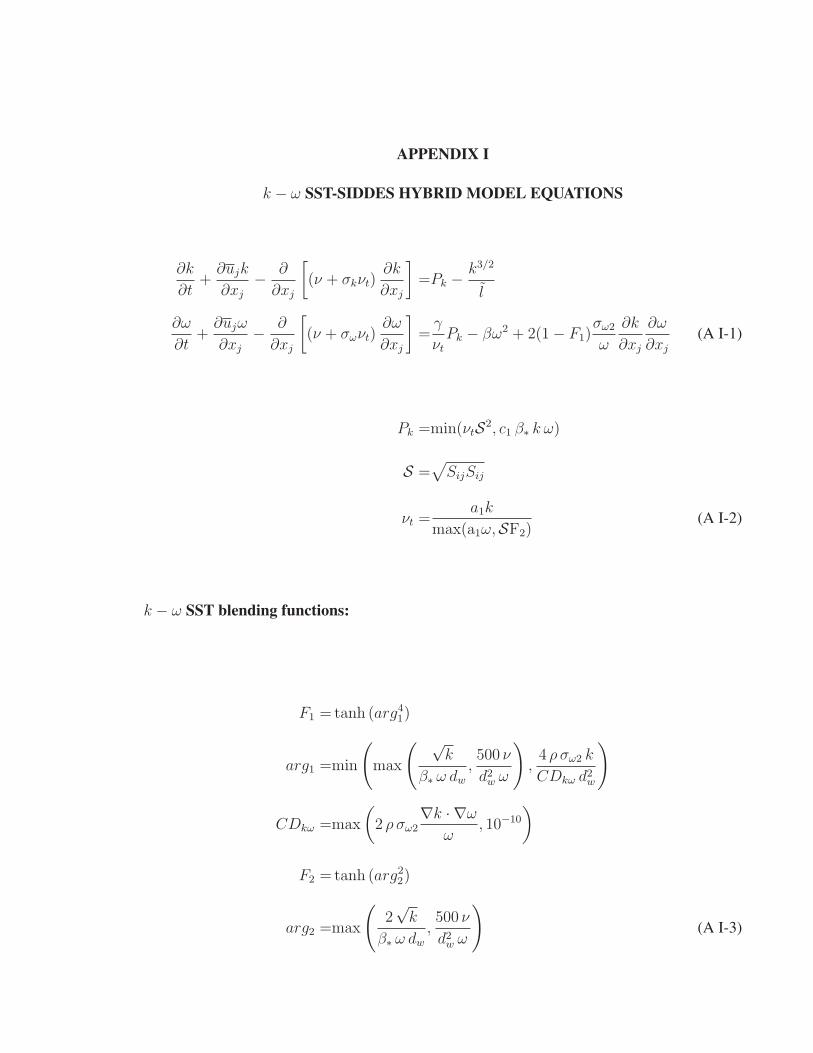
APPENDIX I

k − ω SST-SIDDES HYBRID MODEL EQUATIONS

∂k

∂t+

∂ujk

∂xj

− ∂

∂xj

[(ν + σkνt)

∂k

∂xj

]=Pk − k3/2

l

∂ω

∂t+

∂ujω

∂xj

− ∂

∂xj

[(ν + σωνt)

∂ω

∂xj

]=γ

νtPk − βω2 + 2(1− F1)

σω2

ω

∂k

∂xj

∂ω

∂xj

(A I-1)

Pk =min(νtS2, c1 β∗ k ω)

S =√

SijSij

νt =a1k

max(a1ω,SF2)(A I-2)

k − ω SST blending functions:

F1 =tanh (arg41)

arg1 =min

(max

( √k

β∗ ω dw,500 ν

d2w ω

),4 ρ σω2 k

CDkω d2w

)

CDkω =max

(2 ρ σω2

∇k · ∇ω

ω, 10−10

)

F2 =tanh (arg22)

arg2 =max

(2√k

β∗ ω dw,500 ν

d2w ω

)(A I-3)

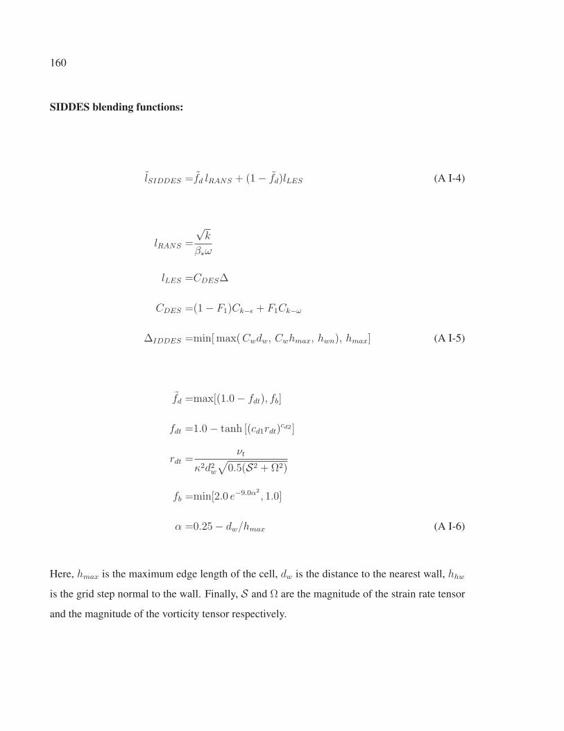
160

SIDDES blending functions:

lSIDDES =fd lRANS + (1− fd)lLES (A I-4)

lRANS =

√k

β∗ω

lLES =CDESΔ

CDES =(1− F1)Ck−ε + F1Ck−ω

ΔIDDES =min[max(Cwdw, Cwhmax, hwn), hmax] (A I-5)

fd =max[(1.0− fdt), fb]

fdt =1.0− tanh [(cd1rdt)cd2 ]

rdt =νt

κ2d2w√

0.5(S2 + Ω2)

fb =min[2.0 e−9.0α2

, 1.0]

α =0.25− dw/hmax (A I-6)

Here, hmax is the maximum edge length of the cell, dw is the distance to the nearest wall, hhw

is the grid step normal to the wall. Finally, S and Ω are the magnitude of the strain rate tensor

and the magnitude of the vorticity tensor respectively.

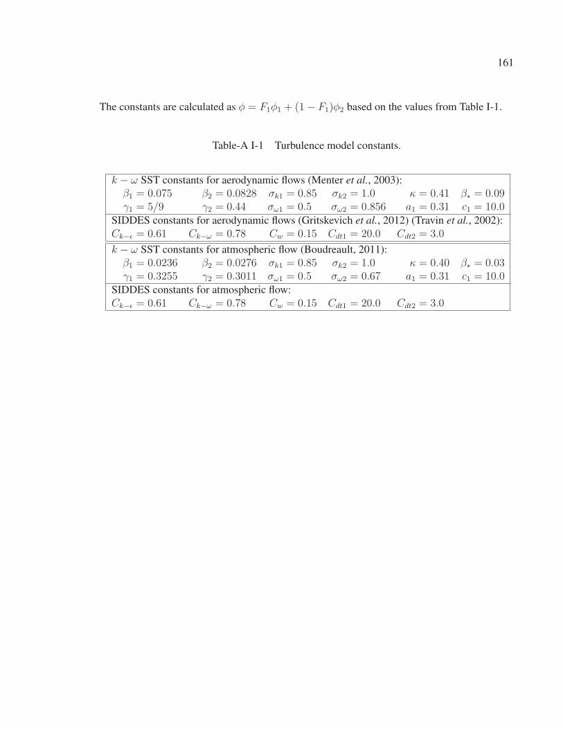
161

The constants are calculated as φ = F1φ1 + (1− F1)φ2 based on the values from Table I-1.

Table-A I-1 Turbulence model constants.

k − ω SST constants for aerodynamic flows (Menter et al., 2003):

β1 = 0.075 β2 = 0.0828 σk1 = 0.85 σk2 = 1.0 κ = 0.41 β∗ = 0.09γ1 = 5/9 γ2 = 0.44 σω1 = 0.5 σω2 = 0.856 a1 = 0.31 c1 = 10.0

SIDDES constants for aerodynamic flows (Gritskevich et al., 2012) (Travin et al., 2002):

Ck−ε = 0.61 Ck−ω = 0.78 Cw = 0.15 Cdt1 = 20.0 Cdt2 = 3.0

k − ω SST constants for atmospheric flow (Boudreault, 2011):

β1 = 0.0236 β2 = 0.0276 σk1 = 0.85 σk2 = 1.0 κ = 0.40 β∗ = 0.03γ1 = 0.3255 γ2 = 0.3011 σω1 = 0.5 σω2 = 0.67 a1 = 0.31 c1 = 10.0

SIDDES constants for atmospheric flow:

Ck−ε = 0.61 Ck−ω = 0.78 Cw = 0.15 Cdt1 = 20.0 Cdt2 = 3.0

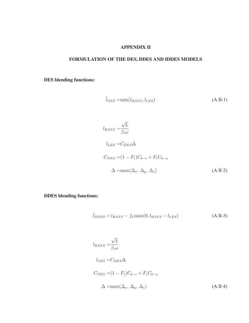
APPENDIX II

FORMULATION OF THE DES, DDES AND IDDES MODELS

DES blending functions:

lDES =min(lRANS, lLES) (A II-1)

lRANS =

√k

β∗ω

lLES =CDESΔ


Δ =max(Δx, Δy, Δz) (A II-2)

DDES blending functions:

lDDES = lRANS − fd max(0, lRANS − lLES) (A II-3)

lRANS =

√k

β∗ω

lLES =CDESΔ


Δ =max(Δx, Δy, Δz) (A II-4)

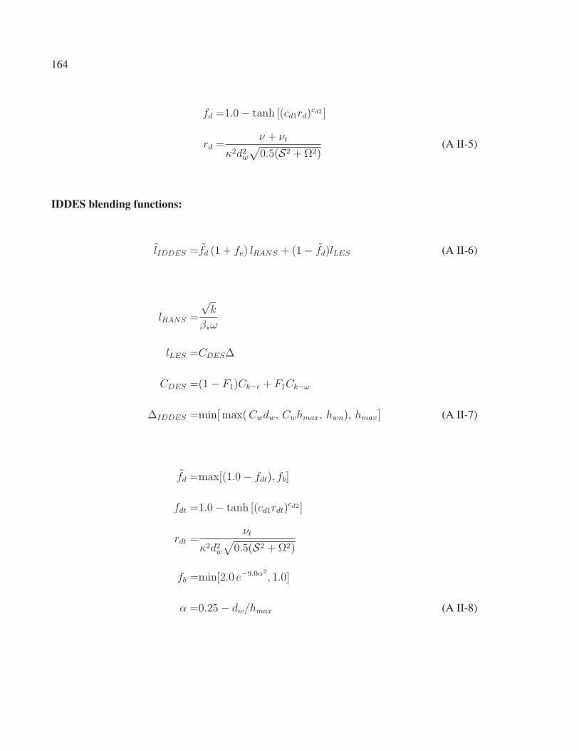
164

fd =1.0− tanh [(cd1rd)cd2 ]

rd =ν + νt

κ2d2w√

0.5(S2 + Ω2)(A II-5)

IDDES blending functions:

lIDDES =fd (1 + fe) lRANS + (1− fd)lLES (A II-6)

lRANS =

√k

β∗ω

lLES =CDESΔ


ΔIDDES =min[max(Cwdw, Cwhmax, hwn), hmax] (A II-7)

fd =max[(1.0− fdt), fb]

fdt =1.0− tanh [(cd1rdt)cd2 ]

rdt =νt

κ2d2w√

0.5(S2 + Ω2)

fb =min[2.0 e−9.0α2

, 1.0]

α =0.25− dw/hmax (A II-8)

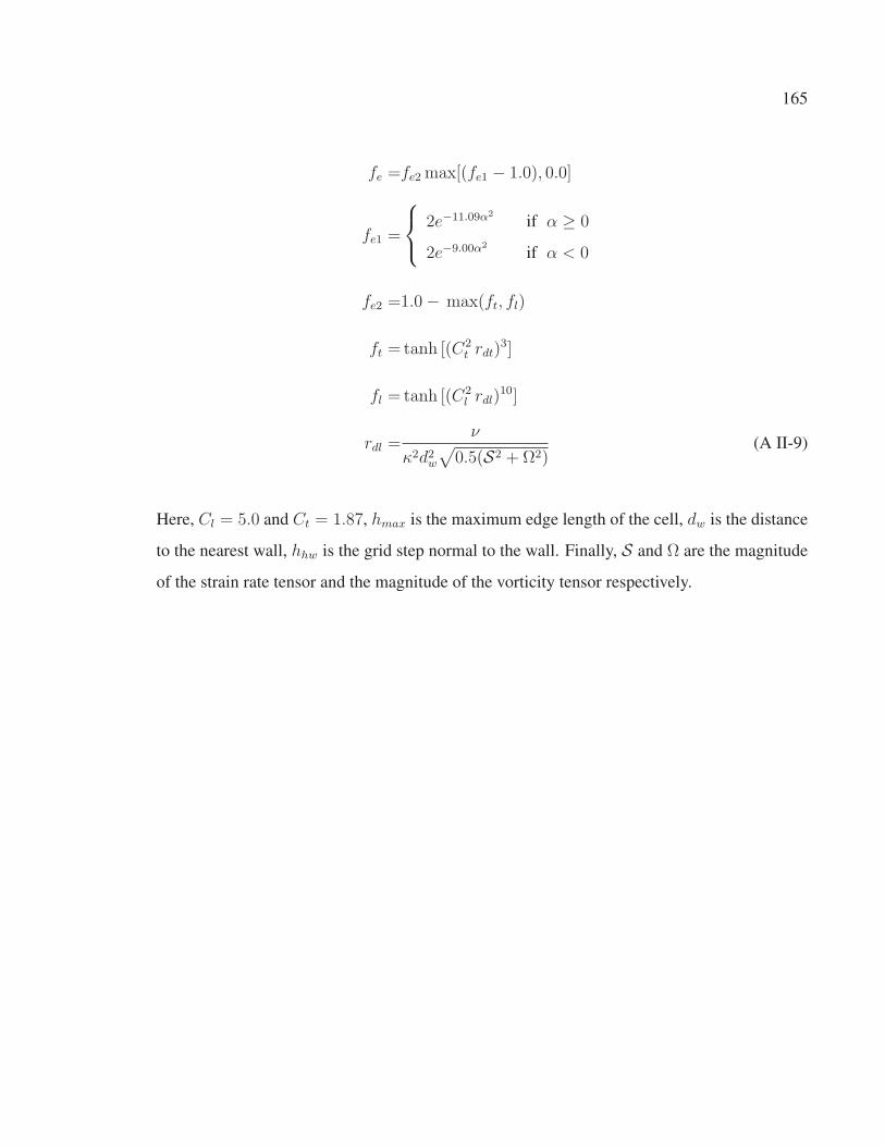
165

fe =fe2 max[(fe1 − 1.0), 0.0]

fe1 =

⎧⎨⎩ 2e−11.09α2if α ≥ 0

2e−9.00α2if α < 0

fe2 =1.0− max(ft, fl)

ft =tanh [(C2t rdt)

3]

fl =tanh [(C2l rdl)

10]

rdl =ν

κ2d2w√

0.5(S2 + Ω2)(A II-9)

Here, Cl = 5.0 and Ct = 1.87, hmax is the maximum edge length of the cell, dw is the distance

to the nearest wall, hhw is the grid step normal to the wall. Finally, S and Ω are the magnitude

of the strain rate tensor and the magnitude of the vorticity tensor respectively.

APPENDIX III

OPENFOAM CODE

1. Implementing the k and ω equations for the hybrid model

// Turbulent frequency equationtmp<fvScalarMatrix> omegaEqn(

fvm::ddt(omega_)+ fvm::div(phi_, omega_)- fvm::Sp(fvc::div(phi_), omega_)- fvm::laplacian(DomegaEff(F1), omega_)==// gamma(F1)*S2 //See Gritskevich2011

gamma(F1)*min(G, c1_*betaStar_*k_*omega_)/max(nuSgs_,dimensionedScalar("SMALL", nuSgs_.dimensions(), SMALL))

- fvm::Sp(beta(F1)*omega_, omega_)- fvm::SuSp

((F1 - scalar(1))*CDkOmega/omega_, omega_

));

.....

// Turbulent kinetic energy equationtmp<fvScalarMatrix> kEqn(

fvm::ddt(k_)+ fvm::div(phi_, k_)- fvm::Sp(fvc::div(phi_), k_)- fvm::laplacian(DkEff(F1), k_)==

min(G, c1_*betaStar_*k_*omega_)//- fvm::Sp(betaStar_*omega_, k_) // Original kwSST code- fvm::Sp(pow(k_,1.0/2.0)/dTilda_, k_) // Modified for SIDDES

);

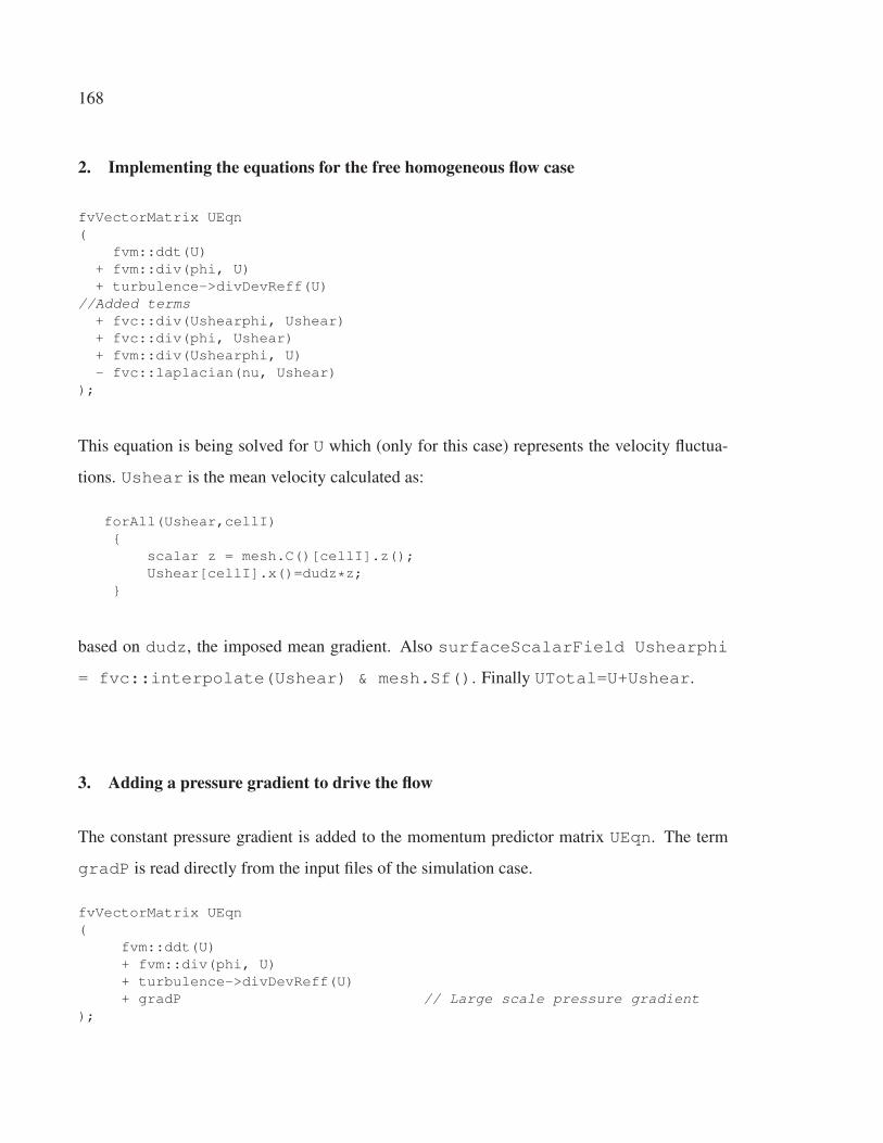
168

2. Implementing the equations for the free homogeneous flow case

fvVectorMatrix UEqn(

fvm::ddt(U)+ fvm::div(phi, U)+ turbulence->divDevReff(U)

//Added terms+ fvc::div(Ushearphi, Ushear)+ fvc::div(phi, Ushear)+ fvm::div(Ushearphi, U)- fvc::laplacian(nu, Ushear)

);

This equation is being solved for U which (only for this case) represents the velocity fluctua-

tions. Ushear is the mean velocity calculated as:

forAll(Ushear,cellI){

scalar z = mesh.C()[cellI].z();Ushear[cellI].x()=dudz*z;

}

based on dudz, the imposed mean gradient. Also surfaceScalarField Ushearphi

= fvc::interpolate(Ushear) & mesh.Sf(). Finally UTotal=U+Ushear.

3. Adding a pressure gradient to drive the flow

The constant pressure gradient is added to the momentum predictor matrix UEqn. The term

gradP is read directly from the input files of the simulation case.

fvVectorMatrix UEqn(

fvm::ddt(U)+ fvm::div(phi, U)+ turbulence->divDevReff(U)+ gradP // Large scale pressure gradient

);

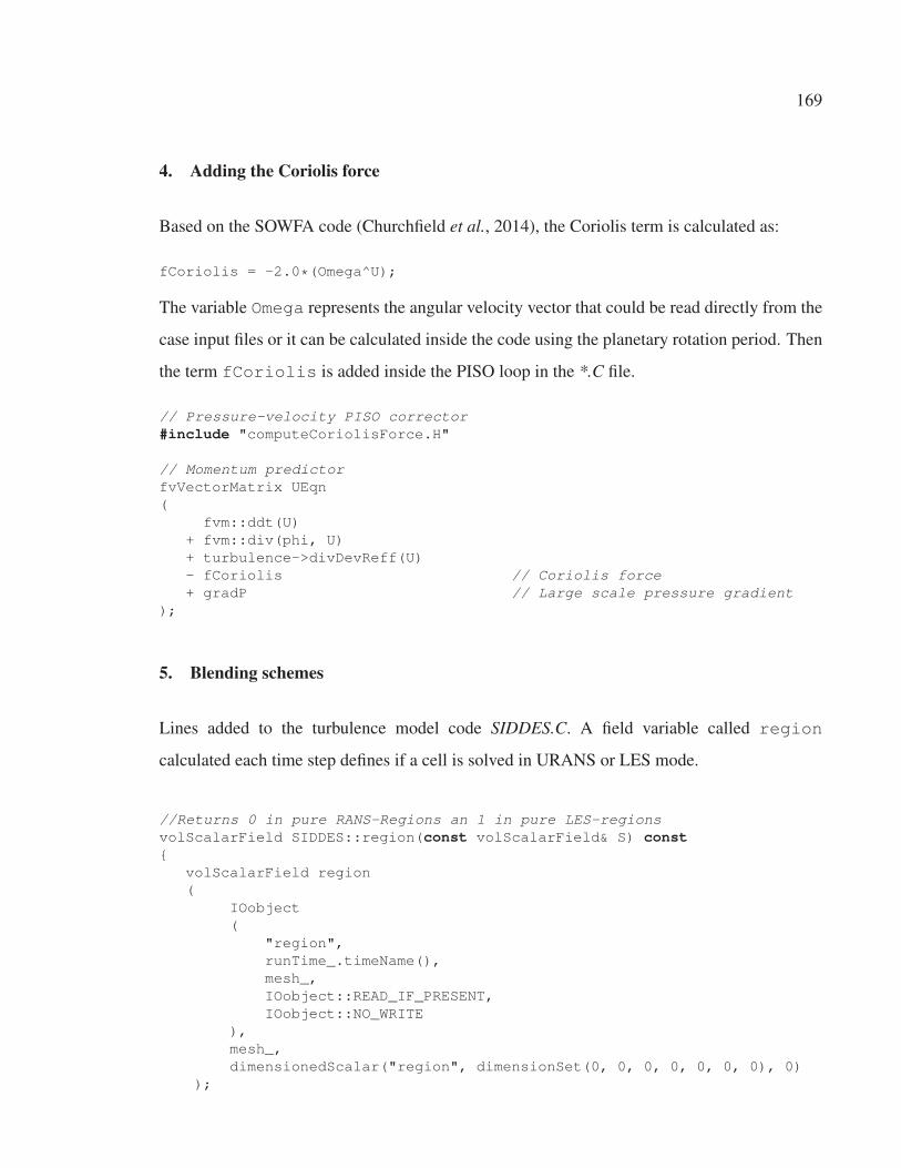
169

4. Adding the Coriolis force

Based on the SOWFA code (Churchfield et al., 2014), the Coriolis term is calculated as:

fCoriolis = -2.0*(Omega^U);

The variable Omega represents the angular velocity vector that could be read directly from the

case input files or it can be calculated inside the code using the planetary rotation period. Then

the term fCoriolis is added inside the PISO loop in the *.C file.

// Pressure-velocity PISO corrector#include "computeCoriolisForce.H"

// Momentum predictorfvVectorMatrix UEqn(

fvm::ddt(U)+ fvm::div(phi, U)+ turbulence->divDevReff(U)- fCoriolis // Coriolis force+ gradP // Large scale pressure gradient

);

5. Blending schemes

Lines added to the turbulence model code SIDDES.C. A field variable called region

calculated each time step defines if a cell is solved in URANS or LES mode.

//Returns 0 in pure RANS-Regions an 1 in pure LES-regionsvolScalarField SIDDES::region(const volScalarField& S) const{

volScalarField region(

IOobject(

"region",runTime_.timeName(),mesh_,IOobject::READ_IF_PRESENT,IOobject::NO_WRITE

),mesh_,dimensionedScalar("region", dimensionSet(0, 0, 0, 0, 0, 0, 0), 0)

);

170

const volScalarField expTerm(exp(sqr(this->alpha())));tmp<volScalarField> fb = min(2*pow(expTerm, -9.0), scalar(1));const volScalarField fdTilda(max(1 - fdt(S), fb));

forAll(fdTilda, cellI){

region[cellI]=1-fdTilda[cellI];}

return region;}

Lines of code added to pisoFoamABL.C file in the solver application. This lines are placed at

the end of the PISO loop to obtain the value of the region from the turbulence model code,

then calculate the blending factors for each needed variable. The blending factor will define

the discretization scheme to use during the following PISO loop.

volScalarField getRegion=mesh.lookupObject<volScalarField>("region");//UBlendingFactor=fvc::interpolate(getRegion);omegaBlendingFactor=fvc::interpolate(getRegion);kBlendingFactor=fvc::interpolate(getRegion);

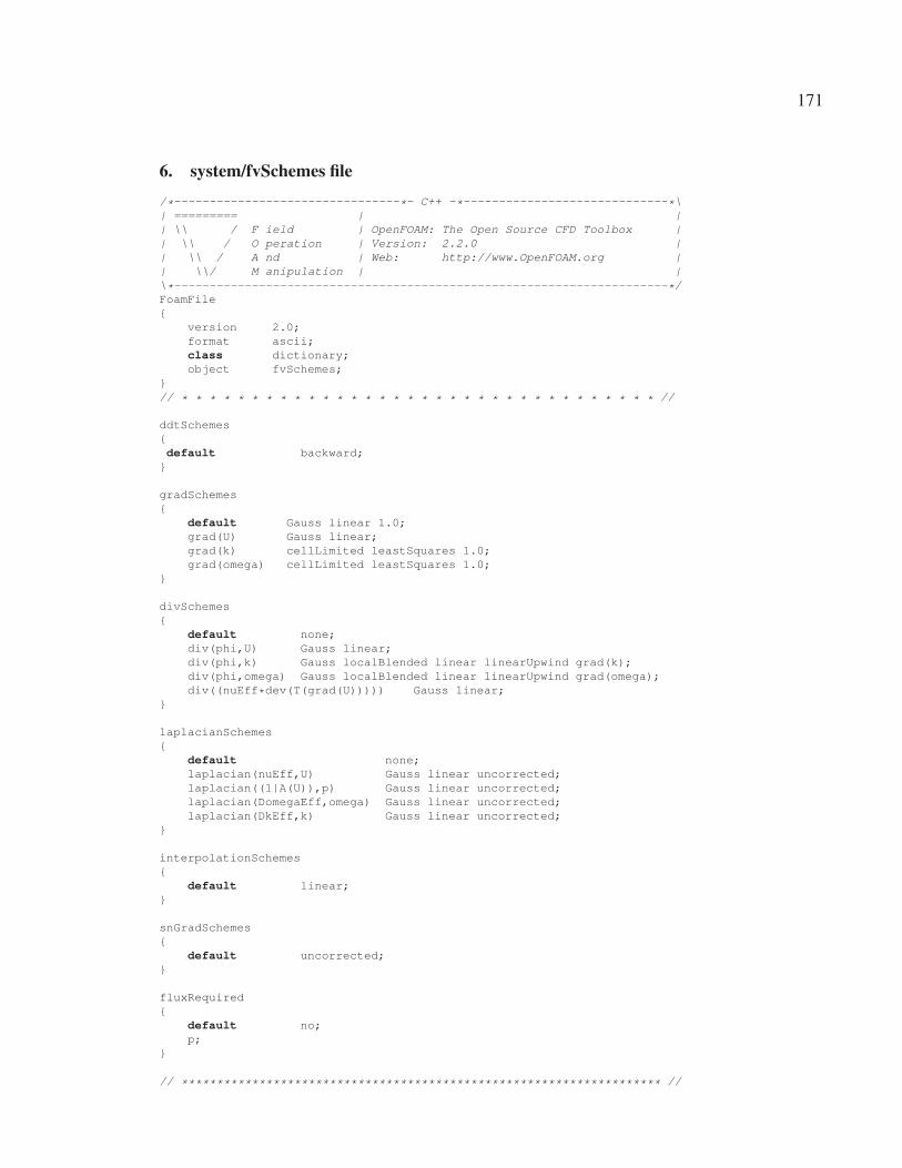
171

6. system/fvSchemes file/*--------------------------------*- C++ -*-----------------------------*\| ========= | || \\ / F ield | OpenFOAM: The Open Source CFD Toolbox || \\ / O peration | Version: 2.2.0 || \\ / A nd | Web: http://www.OpenFOAM.org || \\/ M anipulation | |\*----------------------------------------------------------------------*/FoamFile{

version 2.0;format ascii;class dictionary;object fvSchemes;

}// * * * * * * * * * * * * * * * * * * * * * * * * * * * * * * * * * * //

ddtSchemes{default backward;}

gradSchemes{

default Gauss linear 1.0;grad(U) Gauss linear;grad(k) cellLimited leastSquares 1.0;grad(omega) cellLimited leastSquares 1.0;

}

divSchemes{

default none;div(phi,U) Gauss linear;div(phi,k) Gauss localBlended linear linearUpwind grad(k);div(phi,omega) Gauss localBlended linear linearUpwind grad(omega);div((nuEff*dev(T(grad(U))))) Gauss linear;

}

laplacianSchemes{

default none;laplacian(nuEff,U) Gauss linear uncorrected;laplacian((1|A(U)),p) Gauss linear uncorrected;laplacian(DomegaEff,omega) Gauss linear uncorrected;laplacian(DkEff,k) Gauss linear uncorrected;

}

interpolationSchemes{

default linear;}

snGradSchemes{

default uncorrected;}

fluxRequired{

default no;p;

}

// ******************************************************************** //

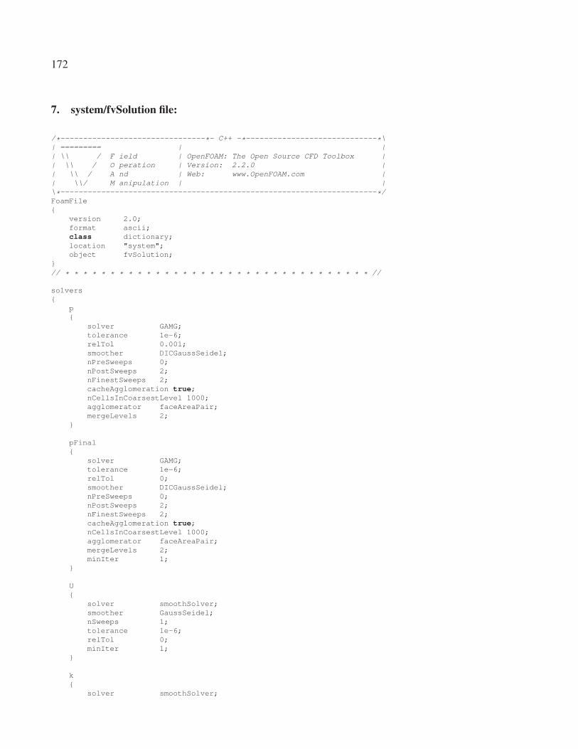
172

7. system/fvSolution file:

/*--------------------------------*- C++ -*-----------------------------*\| ========= | || \\ / F ield | OpenFOAM: The Open Source CFD Toolbox || \\ / O peration | Version: 2.2.0 || \\ / A nd | Web: www.OpenFOAM.com || \\/ M anipulation | |\*----------------------------------------------------------------------*/FoamFile{

version 2.0;format ascii;class dictionary;location "system";object fvSolution;

}// * * * * * * * * * * * * * * * * * * * * * * * * * * * * * * * * * * //

solvers{

p{

solver GAMG;tolerance 1e-6;relTol 0.001;smoother DICGaussSeidel;nPreSweeps 0;nPostSweeps 2;nFinestSweeps 2;cacheAgglomeration true;nCellsInCoarsestLevel 1000;agglomerator faceAreaPair;mergeLevels 2;

}

pFinal{

solver GAMG;tolerance 1e-6;relTol 0;smoother DICGaussSeidel;nPreSweeps 0;nPostSweeps 2;nFinestSweeps 2;cacheAgglomeration true;nCellsInCoarsestLevel 1000;agglomerator faceAreaPair;mergeLevels 2;minIter 1;

}

U{

solver smoothSolver;smoother GaussSeidel;nSweeps 1;tolerance 1e-6;relTol 0;minIter 1;

}

k{

solver smoothSolver;

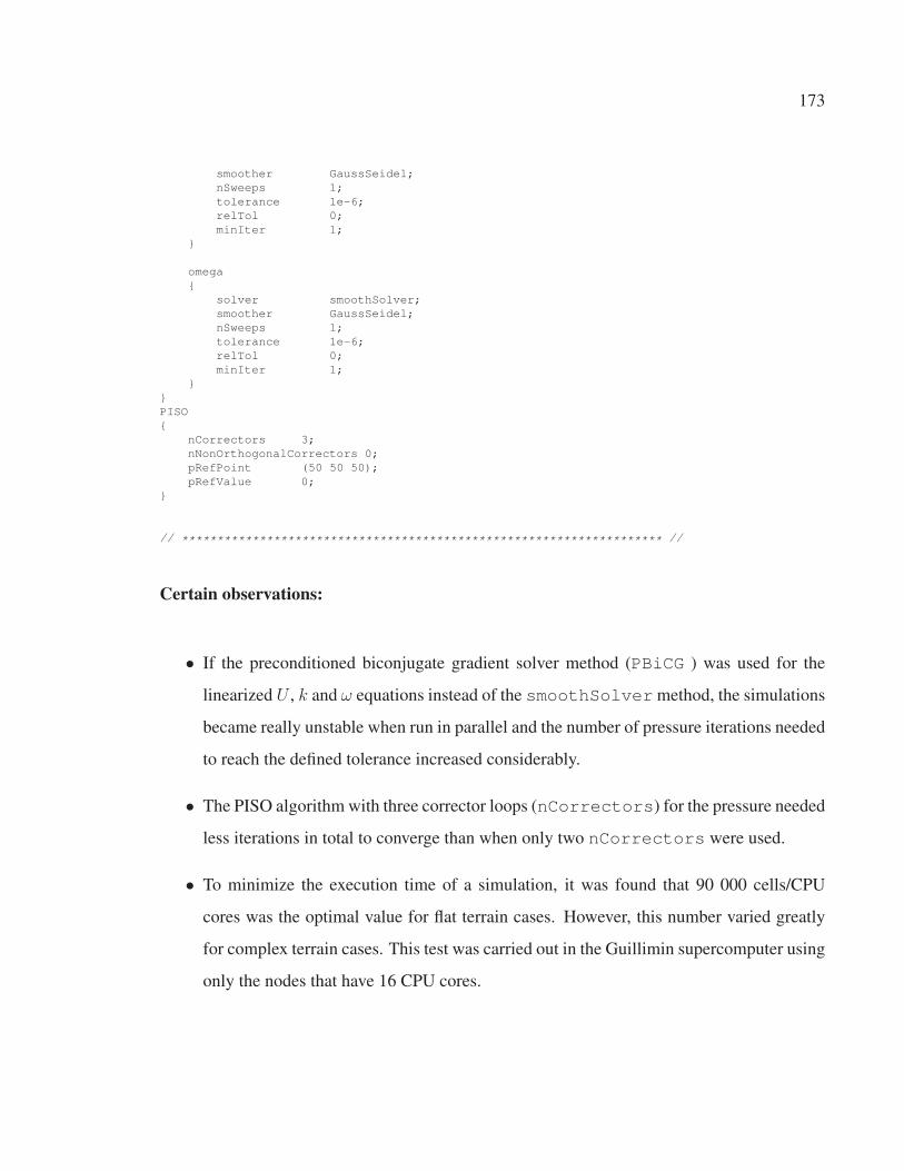
173

smoother GaussSeidel;nSweeps 1;tolerance 1e-6;relTol 0;minIter 1;

}

omega{

solver smoothSolver;smoother GaussSeidel;nSweeps 1;tolerance 1e-6;relTol 0;minIter 1;

}}PISO{

nCorrectors 3;nNonOrthogonalCorrectors 0;pRefPoint (50 50 50);pRefValue 0;

}

// ******************************************************************** //

Certain observations:

• If the preconditioned biconjugate gradient solver method (PBiCG ) was used for the

linearized U , k and ω equations instead of the smoothSolver method, the simulations

became really unstable when run in parallel and the number of pressure iterations needed

to reach the defined tolerance increased considerably.

• The PISO algorithm with three corrector loops (nCorrectors) for the pressure needed

less iterations in total to converge than when only two nCorrectors were used.

• To minimize the execution time of a simulation, it was found that 90 000 cells/CPU

cores was the optimal value for flat terrain cases. However, this number varied greatly

for complex terrain cases. This test was carried out in the Guillimin supercomputer using

only the nodes that have 16 CPU cores.

174

8. Meshing technique in OpenFOAM for complex topography

This meshing technique is based on Jeannotte (2013). To create the Askervien case mesh, two

cases were used: bottomMesh and topMesh. The constant/blockMesh file in the bottom case is

defined as:

*--------------------------------*- C++ -*----------------------------------*\| ========= | || \\ / F ield | OpenFOAM: The Open Source CFD Toolbox || \\ / O peration | Version: 2.2.0 || \\ / A nd | Web: http://www.OpenFOAM.org || \\/ M anipulation | |\*---------------------------------------------------------------------------*/FoamFile{

version 2.2.0;format ascii;class dictionary;object blockMeshDict;

}// * * * * * * * * * * * * * * * * * * * * * * * * * * * * * * * * * * * * * //

convertToMeters 1;

// ******Coordinates of blocksx0 -3800;x1 4000;x2 4000;x3 -3800;

y0 -3200;y1 -3200;y2 2400;y3 2400;

z0 400; //Not really importantz1 500;

//*****Number of cells*****Nx 335; // Number of x-cellsNy 240; // Number of y-cellsNz1 1; // Number of z-cells

//*****Grading values******Gx 1.0; //x-gradingGy 1.0; //y-gradingGz1 1.0 ; //z-grading

vertices(

($x0 $y0 $z0) //0($x1 $y1 $z0) //1($x2 $y2 $z0) //2($x3 $y3 $z0) //3($x0 $y0 $z1) //4($x1 $y1 $z1) //5($x2 $y2 $z1) //6($x3 $y3 $z1) //7

);

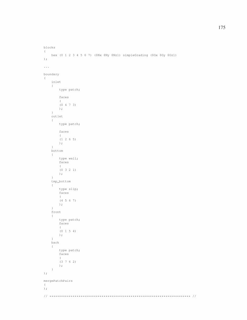
175

blocks(

hex (0 1 2 3 4 5 6 7) ($Nx $Ny $Nz1) simpleGrading ($Gx $Gy $Gz1));

...

boundary(

inlet{

type patch;

faces((0 4 7 3));

}outlet{

type patch;

faces((1 2 6 5));

}bottom{

type wall;faces((0 3 2 1));

}tmp_bottom{

type slip;faces((4 5 6 7));

}front{

type patch;faces((0 1 5 4));

}back{


});

mergePatchPairs();

// ************************************************************************* //

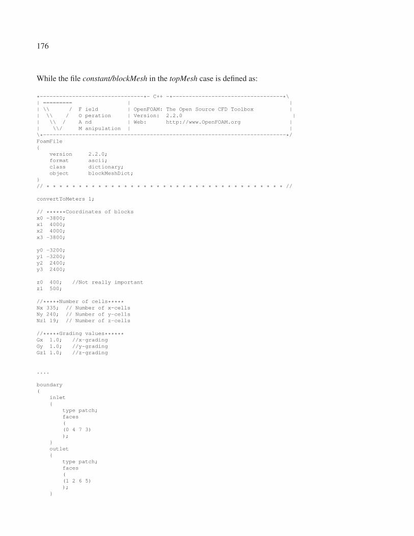
176

While the file constant/blockMesh in the topMesh case is defined as:

*--------------------------------*- C++ -*----------------------------------*\| ========= | || \\ / F ield | OpenFOAM: The Open Source CFD Toolbox || \\ / O peration | Version: 2.2.0 || \\ / A nd | Web: http://www.OpenFOAM.org || \\/ M anipulation | |\*---------------------------------------------------------------------------*/FoamFile{

version 2.2.0;format ascii;class dictionary;object blockMeshDict;

}// * * * * * * * * * * * * * * * * * * * * * * * * * * * * * * * * * * * * * //

convertToMeters 1;

// ******Coordinates of blocksx0 -3800;x1 4000;x2 4000;x3 -3800;

y0 -3200;y1 -3200;y2 2400;y3 2400;

z0 400; //Not really importantz1 500;

//*****Number of cells*****Nx 335; // Number of x-cellsNy 240; // Number of y-cellsNz1 19; // Number of z-cells

//*****Grading values******Gx 1.0; //x-gradingGy 1.0; //y-gradingGz1 1.0; //z-grading

....

boundary(

inlet{


}outlet{


}

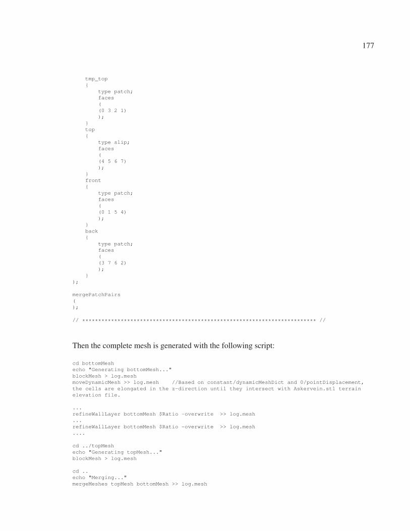
177

tmp_top{


}top{

type slip;faces((4 5 6 7));

}front{


}back{


});

mergePatchPairs();

// ************************************************************************* //

Then the complete mesh is generated with the following script:

cd bottomMeshecho "Generating bottomMesh..."blockMesh > log.meshmoveDynamicMesh >> log.mesh //Based on constant/dynamicMeshDict and 0/pointDisplacement,the cells are elongated in the z-direction until they intersect with Askervein.stl terrainelevation file.

...refineWallLayer bottomMesh $Ratio -overwrite >> log.mesh...refineWallLayer bottomMesh $Ratio -overwrite >> log.mesh....

cd ../topMeshecho "Generating topMesh..."blockMesh > log.mesh

cd ..echo "Merging..."mergeMeshes topMesh bottomMesh >> log.mesh

178

cd topMeshecho "Stitching..."stitchMesh -overwrite -perfect tmp_top tmp_bottom >> log.mesh

echo "Remove tmp patches from constant/polyMesh/boundary file manually!!!!".....

echo "Renumbering ..."renumberMesh >> log.mesh

cp [lastTime]/polyMesh/* constant/polyMesh/rm -rf [lastTime]

echo "The mesh is ready!. Just copy constant/polyMesh/* into the Askervein test case"

This meshing technique can take up to a couple hours to complete for the Askervein case in a

desktop computer.

BIBLIOGRAPHY

Anderson, J. D., 1995. Computational fluid dynamics: the basics with applications. USA :

McGraw-Hill.

Andren, A., A. R. Brown, J. Graf, P. J. Mason, C-H. Moeng, F. T. M. Nieuwstadt, and U. Schu-

mann. 1994. "Large-eddy simulation of a neutrally stratified boundary layer: A compar-

ison of four computer codes". Quarterly Journal of the Royal Meteorological Society,

vol. 120, p. 1457–1484.

Apsley, D. D. and I. P. Castro. 1997. "Flow and dispersion over hills: Comparison between nu-

merical predictions and experimental data". Journal of Wind Engineering and IndustrialAerodynamics, vol. 67 & 68, p. 375–386.

Athanassiadou, M. and I. P. Castro. 2001. "Neutral flow over a series of rough hills: A

laboratory experiment". Boundary-Layer Meteorology, vol. 101, p. 1–30.

Ayotte, K. W. 2008. "Computational modelling for wind energy assessment". Journal of Windengineering and Industrial Aerodynamics, vol. 96, p. 1571-1590.

Bardina, J., J. H. Ferziger, and W. C. Reynolds. May 1983. Improved turbulence models basedon large eddy simulation of homogeneous, incompressible, turbulent flows. Technical

Report TF-19. USA : Thermosciences Division. Department of Mechanical Engineering.

Stanford University.

Bardina, J., J. H. Ferziger, and R. S. Rogallo. 1985. "Effect of rotation on isotropic turbulence:

computation and modelling". Journal of Fluid Mechanics, vol. 154, p. 321–336.

Bartello, P., O. Métais, and M. Lesieur. 1994. "Coherent structures in rotating three-

dimensional turbulence". Journal of Fluid Mechanics, vol. 273, p. 1–29.

Batchelor, G. K., 1967. An introduction to fluid dynamics. Cambridge : Cambridge University

Press.

Bechmann, A. November 2006. "Large-eddy simulation of atmospheric flow over com-

plex terrain". PhD thesis, Risø National Laboratory. Technical University of Denmark,

Roskilde, Denmark. Risø-PhD-28(EN).

Bechmann, A. and N. N. Sørensen. 2010. "Hybrid RANS/LES method for wind flow over

complex terrain". Wind Energy., vol. 13, p. 36-50.

Berg, J., J. Mann, A. Bechmann, M. S. Courtney, and H. E. Jørgensen. 2011. "The Bolund

experiment, Part I: Flow over a steep, three-dimensional hill". Boundary-Layer Meteo-rology, vol. 141, p. 219–243.

Blocken, B., T. Stathopoulos, and J. Carmeliet. 2007. "CFD simulations of the atmospheric

boundary layer: wall function problems". Atmospheric Environment, vol. 41, p. 238-

252.

180

Boudreault, L-É. 2011. "Modélisation numérique de la séparation de l’écoulement atmo-

sphérique". M.Ing thesis, École de Technologie Supérieure, Montreal, QC. Canada.

Bourgeois, J. A., P. Sattari, and R. J. Martinuzzi. 2011. "Alternating half-loop shedding in the

turbulent wake of a finite surface-mounted square cylinder with a thin boundary layer".

Physics of Fluids, vol. 23, n◦ 9, p. 095101.

Boussinesq, M. J., 1897. Théorie de l’écoulement tourbillonnant et tumultueux des liquidesdans les lits rectilignes a grande section. Paris : Gauthier-Villars et fils.

Brasseur, J. G. and T. Wei. 2010. "Designing large-eddy simulation of the turbulent boundary

layer to capture law-of-the-wall scaling". Physics of Fluids, vol. 22, n◦ 2, p. 021303.

Bunge, U., C. Mockett, and F. Thiele. 2007. "Guidelines for implementing detached-eddy

simulation using different models". Aerospace Science and Technology, vol. 11, p. 376–

385.

Castro, F. A., J. M. L. M. Palma, and A. Silva Lopes. 2003. "Simulation of the Askervein

flow. Part 1: Reynolds averaged Navier-Stokes equations (k − ε Turbulence Model)".

Boundary-Layer Meteorology, vol. 107, p. 501-530.

Castro, I. P. and M. Dianat. 1983. "Surface flow patterns on rectangular bodies in thick

boundary layers". Journal of Wind Engineering and Industrial Aerodynamics, vol. 11,

p. 107–119.

Castro, I. P. and A. G. Robins. 1977. "The flow around a surface-mounted cube in uniform and

turbulent streams". Journal of Fluid Mechanics, vol. 79, n◦ 02, p. 307.

Chow, F. K. July 2004. "Subfilter-scale turbulence modeling for large-eddy simulation of the

atmospheric boundary layer over complex terrain". PhD thesis, Department of Civil and

Environmental Engineering, Stanford University, California, USA.

Churchfield, M. J., P. J. Moriarty, G. Vijayakumar, and J. G. Brasseur. August 2-6 2010. "Wind

energy-related atmospheric boundary layer large-eddy simulation using OpenFOAM".

In 19th Symposium on Boundary Layers and Turbulence. (Keystone, Colorado 2010).

Churchfield, M. J., S. Lee, and P. J. Moriarty. 2014. "NREL-NWTC information portal

(SOWFA)". https://nwtc.nrel.gov/SOWFA.

Clifton, A, M H Daniels, and M Lehning. 2014. "Effect of winds in a mountain pass on turbine

performance". Wind Energy, vol. 17, n◦ August 2013, p. 1543–1562.

Comte-Bellot, G. and S. Corrsin. 1971. "Simple eulerian time correlation of full and narrow-

band velocity signals in grid-generated, ‘isotropic’ turbulence". Journal of Fluid Me-chanics, vol. 48, n◦ 2, p. 273-337.

Davidson, P. A., 2004. Turbulence. An introduction for scientists and engineers. Oxford :

Oxford University Press, 657 p.

181

Deardorff, J. W. 1972. "Numerical investigation of neutral and unstable planetary boundary

layers". Journal of the Atmospheric Sciences, vol. 29, p. 91–115.

Detering, H.W. and D. Etling. 1985. "Application of the E-ε turbulence model to the atmo-

spheric boundary layer". Boundary-Layer Meteorology, vol. 33, n◦ 2, p. 113–133.

Drobinski, P. and R. C. Foster. 2003. "On the origin of near-surface streaks in the neutrally-

stratified planetary boundary layer". Boundary-Layer Meteorology, vol. 108, p. 247–

256.

Drobinski, P., P. Carlotti, R. K. Newsom, R. M. Banta, R. C. Foster, and J-L. Redelsperger.

2004. "The structure of the near-neutral atmospheric surface layer". Journal of Atmo-spheric Sciences, vol. 61, p. 699–714.

Drobinski, P., P. Carlotti, J-L. Redelsperger, V. Masson, R. M. Banta, and R. K. Newsom.

2007. "Numerical and experimental investigation of the neutral atmospheric surface

layer". Journal of the Atmospheric Sciences, vol. 64, n◦ 1, p. 137–156.

Emeis, Stefan, 2013. Wind energy meteorology. Atmospheric physics for wind power genera-tion. Berlin : Springer-Verlag.

Ferziger, J.H and M. Peric, 2002. Computational methods for fluid dynamics. ed. 3rd. Berlin :

Springer, 423 p.

Finnigan, J. J. 1988. "Air flow over complex terrain". In Flow and transport in the nat-ural environment: Advances and applications. (Berlin, Germany 1988), p. 183-229.

Springer-Verlag.

Franke, J., A. Hellsten, H. Schlünzen, and B. Carissimo. 2007. Best practice guideline forthe CFD simulation of flows in the urban environment. Technical Report COST Action

732. Quality assurance and improvement of microscale meteorological models. Ham-

burg, Germany : University of Hamburg. Meteorological Institute Centre for Marine and

Atmospheric Sciences.

Garrat, J. R., 1994. The atmospheric boundary layer. Cambridge : Cambridge University

Press.

Godeferd, F. S. 2012. "Relating statistics to dynamics in axisymmetric homogeneous turbu-

lence". Physica D: Nonlinear Phenomena, vol. 241, p. 794–802.

Grant, A. L. M. 1986. "Observations of boundary layer structure made during the 1981

KONTUR experiment". Quarterly Journal of the Royal Meteorological Society, vol.

112, p. 825–841.

Grant, A. L. M. 1991. "The structure of the turbulence in the near neutral atmospheric boundary

layer". Journal of Atmospheric Sciences, vol. 49, n◦ 3, p. 226–239.

182

Gritskevich, M. S., A. V. Garbaruk, J. Schütze, and F. R. Menter. 2012. "Development of DDES

and IDDES formulations for the k − ω shear stress transport model". Flow, Turbulenceand Combustion, vol. 88, p. 431–449.

Gungor, A. G. and S. Menon. 2010. "A new two-scale model for large eddy simulation of

wall-bounded flows". Progress in Aerospace Sciences, vol. 46, p. 28-45.

Hargreaves, D. M. and N. G. Wright. 2007. "On the use of the k−ε model in commercial CFD

software to model the neutral atmospheric boundary layer". Journal of Wind Engineeringand Industrial Aerodynamics, vol. 95, p. 3555-369.

Hinze, J. O., 1975. Turbulence. ed. 2nd. USA : McGraw-Hill.

Hossain, J. and the WWEA Technical Committee. December 2014. World wind resourceassessment report. WWEA Technical Paper Series TP-01-14. Germany : World Wind

Energy Association.

Issa, R. I. 1985. "Solution of the implicitly discretised fluid flow equations by operator-

splitting". Journal of Computational Physics, vol. 62, p. 40–65.

Jackson, P. S. and J. C. R. Hunt. 1975. "Turbulent wind flow over a low hill". Q. J. R. Meteorol.Soc., vol. 101, p. 929–955.

Jeannotte, E. 2013. "Estimation of LIDAR bias over complex terrain using numerical tools".

M.Ing thesis, École de Technologie Supérieure, Montreal, QC. Canada.

Jimenez, A., A. Crespo, and E. Migoya. 2010. "Application of a LES technique to characterize

the wake deflection of a wind turbine in yaw". Wind Energy, vol. 13, p. 559–572.

Jimenez J. (Ed.). 1997. A selection of test cases for the validation of large-eddy simulationsof turbulent flows. Technical Report AGARD Advisory Report No.345. The Fluid

Dynamics Panel : Working Group 21. ftp://torroja.dmt.upm.es/AGARD/.

Kaimal, J. C. and J. J. J. Finnigan, 1994. Atmospheric boundary layer flows. Their structureand measurement. Oxford : Oxford University Press, 283 p.

Kang, H. S., S. Chester, and C. Meneveau. 2003. "Decaying turbulence in an active-grid-

generated flow and comparisons with large-eddy simulation". Journal of Fluid Mechan-ics, vol. 480, p. 129–160.

Katopodes Chow, F. and R. L. Street. 2009. "Evaluation of turbulence closure models for large-

eddy simulation over complex terrain: Flow over Askervein hill". Journal of AppliedMeteorology and Climatology, vol. 48, n◦ 5, p. 1050–1065.

Kim, H. G. and V. C. Patel. 2000. "Test of turbulence models for wind flow over terrain with

separation and recirculation". Boundary-Layer Meteorology, vol. 94, p. 5–21.

183

Knopp, T., B. Eisfeld, and J. B. Calvo. 2009. "A new extension for k-ω turbulence models

to account for wall roughness". International Journal of Heat and Fluid Flow, vol. 30,

n◦ 1, p. 54–65.

Koblitz, T., A. Bechmann, A. Sogachev, N. N. Sørensen, and P. E. Réthoré. 2013. "Com-

putational fluid dynamics model of stratified atmospheric boundary-layer flow". WindEnergy, vol. 18, p. 75–89.

Kolmogorov, A. N. 1941. "The local structure of turbulence in incompressible viscous fluid

for very large Reynolds numbers". Doklady ANSSSR, vol. 30, p. 301-304. (Cited from

Pope, 2000).

Langreder, W., K. Kaiser, H. Hohlen, and J. Hojstrup. 2004. "Turbulence correction for power

curves". EWEC London.

Lee, M. J., J. Kim, and P. Moin. 1990. "Structure of turbulence at high shear rate". Journal ofFluid Mechanics, vol. 216, p. 561–583.

Leonard, A. 1974. "Energy cascade in large-eddy simulations of turbulent fluid flows". Adv.in Geophysics A, vol. 18, p. 237-248.

Lesieur, M. and O. Métais. 1996. "New trends in large-eddy simulations of turbulence". AnnualReview of Fluid Mechanics, vol. 28, p. 45–82.

Lim, H. C., I. P. Castro, and R. P. Hoxey. 2007. "Bluff bodies in deep turbulent boundary

layers: Reynolds-number issues". Journal of Fluid Mechanics, vol. 571, p. 97–118.

Lim, H. C., T. G. Thomas, and I. P. Castro. 2009. "Flow around a cube in a turbulent boundary

layer: LES and experiment". Journal of Wind Engineering and Industrial Aerodynamics,

vol. 97, p. 96–109.

Manwell, J. F., J. G. McGowan, and A. L. Rogers, 2002. Wind energy explained. Theory,design and application. Chippenham, Wiltshire : John Wiley and Sons, LTD.

Mason, P.J. and D J Thomson. 1987. "Large-eddy simulations of the neutral-static-stability

planetary boundary layer". Quarterly Journal of the Royal Meteorological Society, vol.

113, n◦ 476, p. 413–443.

Menter, F. R. 1992. Improved two-equation k-ω turbulence models for aerodynamic flows.

Technical Report NASA-TM-103975. USA : NASA.

Menter, F. R. 1993. "Zonal two equation k − ω turbulence models for aerodynamic flows".

AIAA, vol. 93, p. 2906.

Menter, F. R. 1994. "Two-equation eddy viscosity turbulence models for engineering applica-

tions". AIAA, vol. 32, n◦ 8, p. 1598–1605.

184

Menter, F. R., M. Kuntz, and R. Langtry. 2003. "Ten years of industrial experience with the

SST turbulence model". Turbulence, Heat and Mass Transfer 4, vol. 4, p. 625-632.

Mockett, C., M. Fuchs, and F. Thiele. 2012. "Progress in DES for wall-modelled LES of

complex internal flows". Computers & Fluids, vol. 65, p. 44–55.

Monin, A. S. and A. M. Obukhov. 1954. "Basic laws of turbulent mixing in the atmospheric

surface layer". Trudy Geofiz. Inst. Acad. Sci. U.S.S.R., vol. 24, n◦ 151, p. 163-187.

Muller, Y.-A., Aubrun S., Loyer S., and Masson C. February 4-7th 2013. "Time resolved track-

ing of the far wake meandering of of a wind turbine model in wind tunnel conditions".

In European Wind Energy Association. (Vienna 2013).

Munson, B. R., D. F. Young, and T. H. Okiishi, 2006. Fundamentals of fluid mechanics. ed. 5th.

USA : John Wiley & Sons, Inc.

Nikitin, N. V., F. Nicoud, B. Wasistho, K. D. Squires, and P. R. Spalart. 2000. "An approach to

wall modeling in large-eddy simulations". Physics of Fluids, vol. 12, n◦ 7, p. 1629–1632.

Oberkampf, W. L. and T. G. Trucano. 2002. "Verification and validation in computational fluid

dynamics". Progress in Aerospace Sciences, vol. 38, p. 209-272.

Panofsky, H. A. and J. A. Dutton, 1984. Atmospheric turbulence. Models and methods forengineering applications. USA : John Wiley & Sons, Inc.

Panton, R. L., 1995. Incompressible flow. ed. 2nd. USA : Wiley-Interscience Publication,

837 p.

Patankar, S. V., 1980. Numerical heat transfer and fluid flow. USA : Taylor & Francis.

Patel, V. C. 1998. "Perspective: flow at high Reynolds number and over rough surfaces -

Achilles heel of CFD". Journal of Fluid Engineering, vol. 120, p. 434–444.

Patel, V. C. and J. Y. Yoon. 1996. "Application of turbulence models to separated flow over

rough surfaces". Journal of Fluid Engineering, vol. 117, p. 234 – 241.

Peña, A., R. Floors, and S-E. Gryning. 2014. "The Høvsøre tall wind-profile experiment: A

description of wind profile observations in the atmospheric boundary layer". Boundary-Layer Meteorology, vol. 150, p. 69–89.

Peinke, J., S. Barth, F. B ottcher, D. Heinemann, and B. Lange. 2004. "Turbulence, a challeng-

ing problem for wind energy". Physics A, vol. 338, p. 187-193.

Peng-Karrholm, Fabian. 2006. Rhie-Chow interpolation in OpenFOAM. Technical report.

Göteborg, Sweden : Chalmers University of Technology.

Petersen, E. L., N. G. Mortensen, L. Landberg, J. Højstrup, and H. P. Frank. 1998. "Wind

power meteorology. Part II: Sitting and models". Wind Energy, vol. 1, p. 55-72.

185

Piomelli, U., J. Ferziger, and P. Moin. 1989. "New approximate boundary conditions for large

eddy simulations of wall-bounded flows". Phys. Fluids A, vol. 1, n◦ 6, p. 1061–1068.

Pope, S. B. 1975. "A more general effective-viscosity hypothesis". Journal of Fluid Mechanics,

vol. 72, p. 331–340.

Pope, S. B., 2000. Turbulent flows. Cambridge : Cambridge University Press, 771 p.

Porté-Agel, F., C. Meneveau, and M. B. Parlange. 2000. "A scale-dependent dynamic model

for large-eddy simulation: application to a neutral atmospheric boundary layer". Journalof Fluid Mechanics, vol. 415, p. 261-284.

Pumir, A. 1996. "Turbulence in homogeneous shear flows". Physics of Fluids, vol. 8, n◦ 11, p.

3112–3127.

Reichardt, H. 1951. "Vollständige darstellung der turbulenten geschwindigkeitsverteilung in

glatten leitungen". ZAMM - Journal of Applied Mathematics and Mechanics. Zeitschriftfür Angewandte Mathematik und Mechanik, vol. 31, n◦ 7, p. 208–219.

Reynolds, O. 1895. "On the dynamical theory of incompressible viscous fluids and the deter-

mination of the criterion". Phil Trans. R. Lond. Soc. A., vol. 186, p. 123–164.

Richards, P. and R. Hoxey. 1993. "Appropriate boundary conditions for computational wind

engineering models using the k−ε model". Journal of Wind Engineering and IndustrialAerodynamics, vol. 46 & 47, p. 145-153.

Riziotis, V. A. and S. G. Voustsinas. 2000. "Fatigue loads on wind turbines of different control

strategies operating in complex terrain". Journal of Wind Engineering and IndustrialAerodynamics, vol. 85, p. 211-240.

Rogallo, S. 1981. Numerical experiments in homogeneous turbulence. Technical Report

NASA-TM-81315. USA : NASA.

Rogers, M. M. and P. Moin. 1987. "The structure of the vorticity field in homogeneous

turbulent flows". Journal of Fluid Mechanics, vol. 176, p. 33–66.

Roy, C. J., L. J. Dechant, J. L. Payne, and F. G. Blottner. 2003. "Bluff-body flow simulations

using hybrid RANS/LES". AIAA Journal, vol. 3889.

Sagaut, P., 2006. Large eddy simulations for incompressible flows: An introduction. ed. 3rd.

Berlin : Springer.

Sagaut, P. and C. Cambon, 2008. Homogeneous turbulence dynamics. Cambridge : Cambridge

University Press, 460 p.

Sakamoto, H. 1983. "Vortex shedding from a rectangular prism and a circular cylinder placed

vertically in a turbulent boundary layer". Journal of Fluid Mechanics, vol. 126, p. 147–

165.

186

Salmon et. al., J. R. 1988. "The Askervein hill project: mean wind variations at fixed heights

above ground". Boundary-Layer Meteorology, vol. 43, p. 247-271.

Sanz Rodrigo, J. et al. 2014. "IEA-Task 31 Wakebench: Towards a protocol for wind farm

flow model evaluation. Part 1: Flow-over-terrain models". The Science of Making Torquefrom Wind 2014. Journal of Physics: Conference Series., vol. 524, p. 012105.

Sanz Rodrigo, J. et al. 2014. "IEA-Wind Task 31 "Wakebench" project. Windbench portal.".

https://windbench.net.

Sattari, P., J. A. Bourgeois, and R. J. Martinuzzi. 2011. "On the vortex dynamics in the wake

of a finite surface-mounted square cylinder". Experiments in Fluids, vol. 52, n◦ 5, p.

1149–1167.

Schlichting, H. and K. Gersten, 2000. Boundary layer theory. ed. 8th. Berlin : Springer.

Senocak, I., A. S. Ackerman, M. P. Kirkpatrick, D. E. Stevens, and N. N. Mansour. 2007.

"Study of near-surface models for large-eddy simulations of a neutrally stratified atmo-

spheric boundary layer". Boundary-Layer Meteorology, vol. 124, p. 405-424.

Shur, M. L., P. R. Spalart, M. Kh. Strelets, and A. K. Travin. 2008. "A hybrid RANS-LES

approach with delayed-DES and wall-modelled LES capabilities". International Journalof Heat and Fluid Flow, vol. 29, n◦ 6, p. 1638–1649.

Silva Lopes, A., J. M. L. M. Palma, and F. A. Castro. 2007. "Simulation of the Askervein flow.

Part 2: Large-eddy simulations". Boundary-Layer Meteorology, vol. 125, p. 85-108.

Sørensen, N. N. 1995. General purpose flow solver applied to flow over hills. Risø-R-827(EN).

Roskilde, Denmark : RisøNational Laboratory.

Spalart, P. R. July 2001. Young-person’s guide to detached-eddy simulation grids. Technical

Report CR-2001-211032. USA : NASA.

Spalart, P. R., W-H. Jou, M. Strelets, and S.R. Allmaras. August 4-8 1997. "Comments on

the feasibility of LES for wings, and on a hybrid RANS/LES approach". In Proceedingsof the first AFOSR international conference on DNS/LES. (Ruston, Louisiana 1997).

Louisiana Tech University.

Spalart, P. R., S. Deck, M. L. Shur, K. D. Squires, M. K. Strelets, and A. Travin. 2006. "A new

version of detached-eddy simulation, resistant to ambiguous grid densities". Theoreticaland Computational Fluid Dynamics, vol. 20, n◦ 3, p. 181-195.

Stoll, R. and F. Porté-Agel. 2006. "Effect of roughness on surface boundary conditions for

large-eddy simulation". Boundary-Layer Meteorology, vol. 118, p. 169–187.

Stull, R. B., 1988. An introduction to boundary layer meteorology. Dordrecht : Kluwer

Academic Publishers.

187

Sukheswalla, P., T. Vaithianathan, and L. R. Collins. 2013. "Simulation of homogeneous

turbulent shear flows at higher Reynolds numbers: numerical challenges and a remedy".

Journal of Turbulence, vol. 14, n◦ 5, p. 60–97.

Sullivan, P. P. 1994. "A subgrid-scale model for large-eddy simulation of planetary boundary-

layer flows". Boundary-Layer Meteorology, vol. 71, p. 247–276.

Sumner, J. and C. Masson. 2012. "The Apsley and Castro limited-length-scale k − ε model

revisited for improved performance in the atmospheric surface Layer". Boundary-LayerMeteorology, vol. 144, n◦ 2, p. 199-215.

Sumner, J., C. S. Watters, and C. Masson. 2010. "Review. CFD in wind energy: The virtual,

multiscale wind tunnel". Energies, vol. 3, p. 989-1013.

Tavoularis, S. and U. Karnik. 1989. "Further experiments on the evolution of turbulent stresses

and scales in uniformly sheared turbulence". Journal of Fluid Mechanics, vol. 204, p.

457–478.

Taylor, P. A. and H. W. Teunissen. November 1983. Askervein ’82: Report on the Septem-ber/October 1982 experiment to study boundary-layer flow over Askervein, South Uist.Technical Report MSRB-83-8. Canada : Environment Canada. Atmospheric Environ-

ment Service.

Taylor, P. A. and H. W. Teunissen. December 1985. The Askervein hill project: Report onthe Sept./Oct. 1983, Main field experiment. Technical Report MSRB-84-6. Canada :

Environment Canada. Atmospheric Environment Service.

Taylor, P. A. and Teunissen H. W. 1987. "The Askervein hill project: Overview and background

data". Boundary-Layer Meteorology, vol. 39, p. 15-39.

Tennekes, H. and J. L. Lumley, 1972. A first course in turbulence. Cambridge, Massachusetts :

The MIT Press, 300 p.

The OpenFOAM Foundation. 28th September 2013. "OpenFOAM R© - The open source CFD

toolbox. User guide". http://www.openfoam.org.

The WRF community. 2015. "The weather research and forecasting model website".

http://www.wrf-model.org/.

Travin, A., M. L. Shur, M. Strelets, and P. R. Spalart. 2002. "Physical and numerical upgrades

in the detached-eddy simulation of complex turbulent flows.". In Advances in LES ofComplex Flows Conference Proceedings. (Printed in the Netherlands 2002), p. 239-254.

KluwerAcademic Publishers.

Troldborg, N. June 2008. "Actuator line modeling of wind turbine wakes". PhD thesis, Depart-

ment of Mechanical Engineering, Technical University of Denmark, Lyngby, Denmark.

188

Uchida, T. and Y. Ohya. 2003. "Large-eddy simulation of turbulent airflow over complex

terrain". Journal of Wind Engineering and Industrial Aerodynamics, vol. 91, p. 219-

229.

Versteeg, H. K. and W. Malalasekera, 2007. An introduction to computational fluid dynamics.The finite volume method. ed. 2nd. Harlow : Pearson Education Limited, 503 p.

Wang, H. F., Y. Zhou, C. K. Chan, and K. S. Lam. 2006. "Effect of initial conditions on

interaction between a boundary layer and a wall-mounted finite-length-cylinder wake".

Physics of Fluids, vol. 18, p. 065106.

Welch, P. D. 1967. "The use of fast Fourier transform for the estimation of power spectra: A

method based on time averaging over short, modified periodograms". IEEE Transactionson Audio and Electroacoustics, vol. AU-15, p. 70–73.

White, F. M., 1991. Viscous fluid flow. McGraw-Hill Series in Mechanical Engineering.

ed. 2nd. Boston : McGraw-Hill.

Wilcox, D. C., 2004. Turbulence modeling for CFD. ed. 2nd. San Diego, California : Birm-

ingham Press, Inc., 540 p.

Wood, N. 2000. "Wind Flow over Complex Terrain: A Historical perspective and the prospect

for Large-Eddy Modelling". Boundary-Layer Meteorology, vol. 96, p. 11-32.

World Wind Energy Association. 2014. "World wind energy half-year report 2014".

http://www.wwindea.org.

Yu, H., S. S. Girimaji, and L-S. Luo. 2005. "DNS and LES of decaying isotropic turbulence

with and without frame rotation using lattice Boltzmann method". Journal of Computa-tional Physics, vol. 209, p. 599–616.

Documents

ÉCOLE DE TECHNOLOGIE SUPÉRIEURE …espace.etsmtl.ca/1570/2/BAUTISTA_Mary_Carmen-web.pdf · La ﬁnesse verticale de la grille de calcul proche des limites du ... Mot-clés: technologíe