ECO 120 Macroeconomics

Week 2

Aggregate Expenditures Model LecturerDr. Rod Duncan

News

• Tutorials begin this week. The tutorial lists are on the class webpage and on the wall outside Rod’s office C2-232.

• There is a second tutorial (T9) on Tuesday 5-6pm for Jim Browning in C2-206.

Topics

• Measurement of GDP (what does it represent and how do we measure it?)

• Two sector AE model

• Consumption functions

• Savings functions

Why measure GDP?

• What are the goals of economics?– Answer: Achieve the greatest happiness (welfare or

utility) for individuals in society.– Problem: We can’t measure happiness.

• Second best: We measure the resources and opportunities available to members of society.– We assume that happiness is related to the range of

choices individuals have within society. The more choices people have, the more likely they are to find a choice they are happy with.

Measures of economic output

• Gross domestic product- The total market value of all final goods and services produced in a period (usually the year) within a country.

• Gross national product- The total market value of all final goods and services produced in a period (usually the year) by Australians. – So an Australian lawyer working overseas for 6

months would include his overseas earnings as Aussie GNP but not Aussie GDP.

• Important: GDP/GNP figures use “market prices” to value things and do not count intermediate goods.

Why measure GDP?

• We can’t measure the range of choices, so we measure the value of what we produce and assume that a greater value of production meant that we had more opportunities.

• Paradox of happiness: Richer people report themselves as happier than poorer people. But average happiness in rich societies is not greater than average happiness in poor societies.– So how can we say we are measuring happiness

when more GDP does not make people happier?

Does GDP = happiness?

• Citizens of richer countries generally:– Lead longer, healthier lives;– Are better educated and spend more years in

education;– Have more leisure time and opportunities;– Have greater levels of political participation;– Lead less risky lives from natural or man-made

disasters;– Breathe cleaner air and drink cleaner water;– …

• So perhaps asking people about their “happiness” is not the right question.

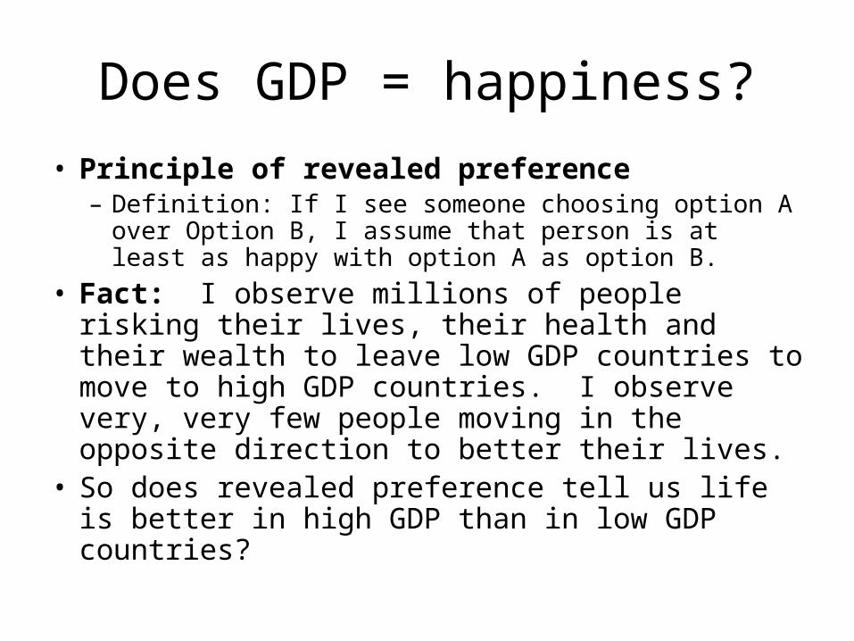
Does GDP = happiness?

• Principle of revealed preference– Definition: If I see someone choosing option A over

Option B, I assume that person is at least as happy with option A as option B.

• Fact: I observe millions of people risking their lives, their health and their wealth to leave low GDP countries to move to high GDP countries. I observe very, very few people moving in the opposite direction to better their lives.

• So does revealed preference tell us life is better in high GDP than in low GDP countries?

Problems with using GDP measures

• We assume that higher GDP is better.• But is GDP the right way to measure economic

output?• GDP only counts things which are valued in

markets- so have market prices.– If we dirty our water, pollution is generally unpriced,

so this would not come into GDP calculations.– A parent taking care of his or her own children is not

paid in the market, so is not counted as part of GDP.– Black market/illegal activities are not measured or

counted as part of GDP.

Measurement of GDP

• Example: In the 1980s, Italy engaged in major reforms of its regulatory practices- slashing a lot of red tape. Italian GDP growth rates were among the highest in Europe. So can we say that Italian reforms greatly increased the welfare of Italians?– Problem: Much of the expansion in GDP was simply

new reporting from firms that had been operating in the black market due to the difficulty of regulations becoming “legit” after the reforms. This was not new output.

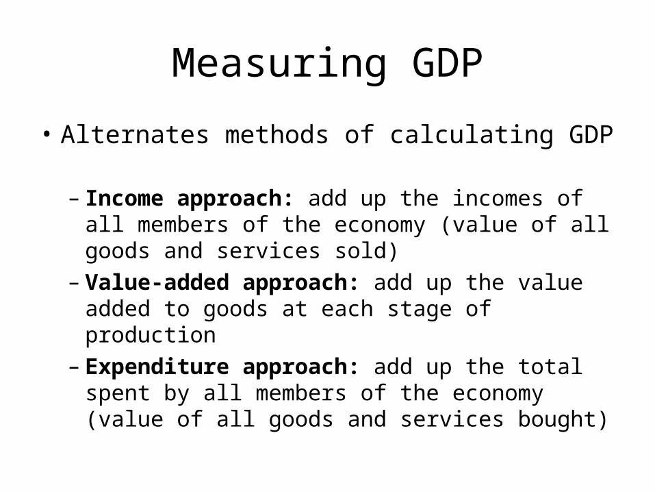
Measuring GDP

• Alternates methods of calculating GDP– Income approach: add up the incomes of all

members of the economy (value of all goods and services sold)

– Value-added approach: add up the value added to goods at each stage of production

– Expenditure approach: add up the total spent by all members of the economy (value of all goods and services bought)

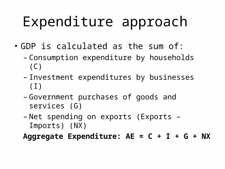
Expenditure approach

• GDP is calculated as the sum of:– Consumption expenditure by households (C)– Investment expenditures by businesses (I)– Government purchases of goods and services

(G)– Net spending on exports (Exports – Imports)

(NX)

Aggregate Expenditure: AE = C + I + G + NX

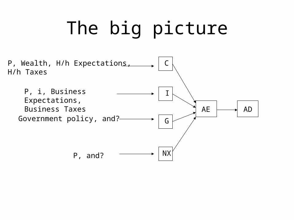
The big picture

P, Wealth, H/h Expectations,H/h Taxes

P, i, Business Expectations, Business Taxes

C

Government policy, and? G

P, and? NX

AE AD

I

Goods market

• Just as in microeconomics, we will model a market for “goods” (this is really shorthand for all goods and services sold in the economy).

• Demand: Goods demand is the purchase of all goods- AE = C + I + G + NX

• Supply: Goods supply is the value of all goods produced- Y

• Equilibrium: We have equilibrium in the goods market when demand is equal to supply:

Y = AE = C + I + G + NX

Two sector model

• The simplest model of the goods market is the two sector model, where goods demand is C and I- private consumption and investment demand.

• In this simplest model, we do not have a government sector (so no G and no taxes), and we do not have trade with the outside world (so no NX).

• We have equilibrium Y* when goods supply, Y, is equal to goods demand, C + I, so what determines C and I?

Two sector model

• C is assumed to be a function of Y- economists usually write this as C = C(Y).– C(Y) tells us the value of C for every value of Y.– C increases as Y increases.– The equilibrium value of C* will depend on the

equilibrium value of Y, Y*. C is an “endogenous” variable- determined within the model.

– One simple form would be that C is a linear function of Y, so

C(Y) = a + b Y

– Since C is increasing in Y, b > 0.

Properties of a consumption function

• What assumptions are we going to make about aggregate consumption of goods and services in an economy?– An aggregate consumption function is simply adding

up all consumption functions of all individuals in society.

– If personal income is 0, people consume a positive amount, through using up savings, borrowing from others, etc, so C(0) should be greater than 0.

– As personal income rises, people spend more, so the slope of C(Y) should be positive.

A consumption function

Can we graph this?

Y

C(Y)

Y*

C(Y*)

C(0)

A consumption function could look like this.

A linear consumption function

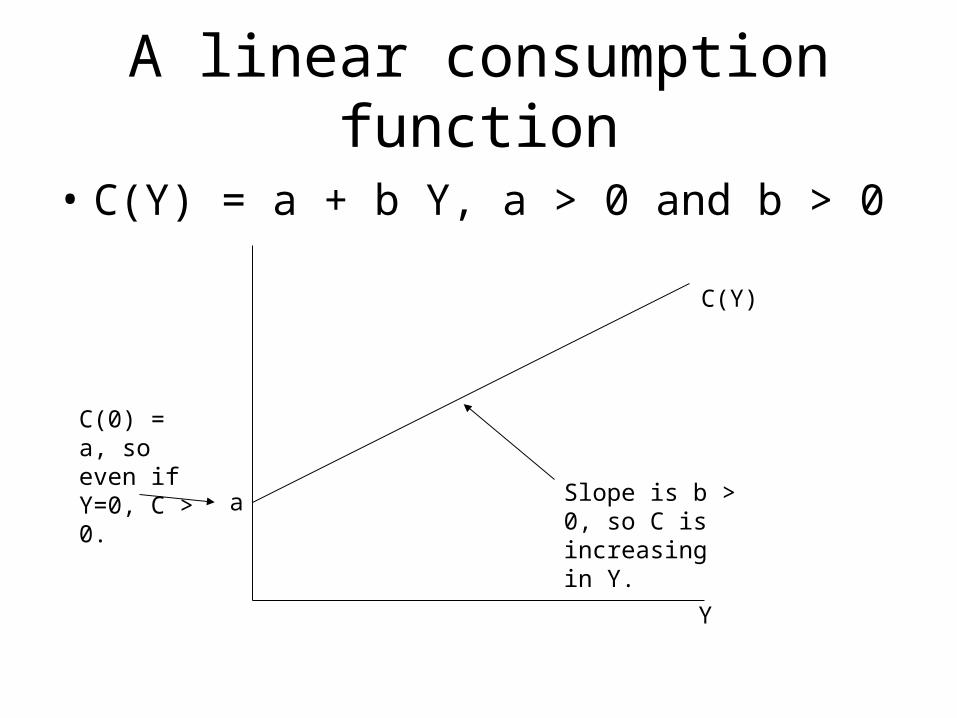
• C(Y) = a + b Y, a > 0 and b > 0

Y

C(Y)

a Slope is b > 0, so C is increasing in Y.

C(0) = a, so even if Y=0, C > 0.

Graphing a function in Excel

• This subject use a lot of “quantitative data” (which means lists of numbers measuring things).

• Students will need to develop their quantitative skills-– Graphing data– Using data to support an argument– Modelling in Excel

• We will be using Excel during this subject. You must become familiar with Excel.

Investment

• In the two sector model, we assume that I is a fixed value, such as $40 billion.– Investment does not depend on Y.– The equilibrium value of I is determined

outside the model, so I is called an “exogenous” variable.

– Later in the subject, we will allow I to vary and discuss the factors that influence I.

Savings

• Y is the total value of production, but Y is also the total value of income in the economy. All sales have to end up as someone’s income.– Sales from a company end up paying worker wages

or as income to the owners of the company.

• If Y is income and C of income is spent, then Y – C is saved, so we must also have a savings function, S(Y), which relates the aggregate level of savings to aggregate income.

• What are the properties of this S(Y)?

Savings function

• Just as with consumption, aggregate savings in an economy should be the sum of every individual’s savings function.

• At very low levels of income, people will borrow (negative savings) rather than starve, so S(0) < 0.

• As income rises, people consume some and save some of their incomes, so S(Y) should be increasing in Y.

• Can we use this knowledge to graph an aggregate savings function?

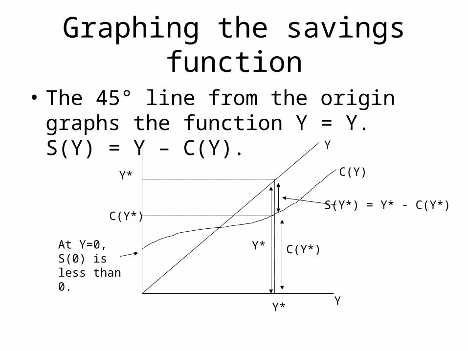
Graphing the savings function

• The 45° line from the origin graphs the function Y = Y. S(Y) = Y – C(Y).

Y

Y

C(Y)

Y*

Y*

C(Y*)

C(Y*)Y*

S(Y*) = Y* - C(Y*)

At Y=0, S(0) is less than 0.

A linear savings function

• If C(Y) is linear, then S(Y) = Y - a - bY, or S(Y) = -a + (1-b) Y, which is also a linear function.

• We assume that if income rises, people consume a part of the increase and save a part of the increase. This means that:

0 < b < 1 and 0 < (1-b) < 1.

• The savings function will then have a negative vertical intercept (at –a) and a positive slope (1-b).

• So what does a linear savings function look like?

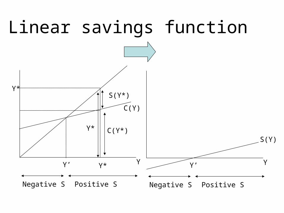
Linear savings function

Y

C(Y)

Y*

Y*

C(Y*)Y*

S(Y*)

Y’

Negative S Positive S

Y

S(Y)

Y’

Negative S Positive S

Average propensity

• Average Propensity to Consume (APC) is consumption as a fraction of Y:

APC = C / Y• Average Propensity to Save (APS) is

savings as a fraction of Y:APS = S / Y

• Since all income is either consumed or saved, we have:

APC + APS = 1

Marginal propensity

• Marginal Propensity to Consume (MPC) is the change in consumption as Y changes:

MPC = (Change in C) / (Change in Y)

• Marginal Propensity to Save (APS) is the change in savings as Y changes:

MPS = (Change in S) / (Change in Y)

Marginal propensity

• For our linear consumption and savings functions, MPC = b and MPS = (1-b). If Y changes, then consumption and savings must change to use up all the change in Y, so

MPC + MPS = 1.

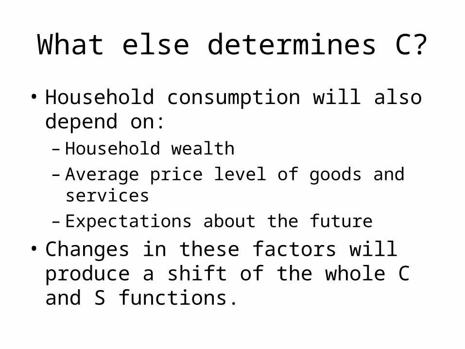
What else determines C?

• Household consumption will also depend on:– Household wealth– Average price level of goods and services– Expectations about the future

• Changes in these factors will produce a shift of the whole C and S functions.

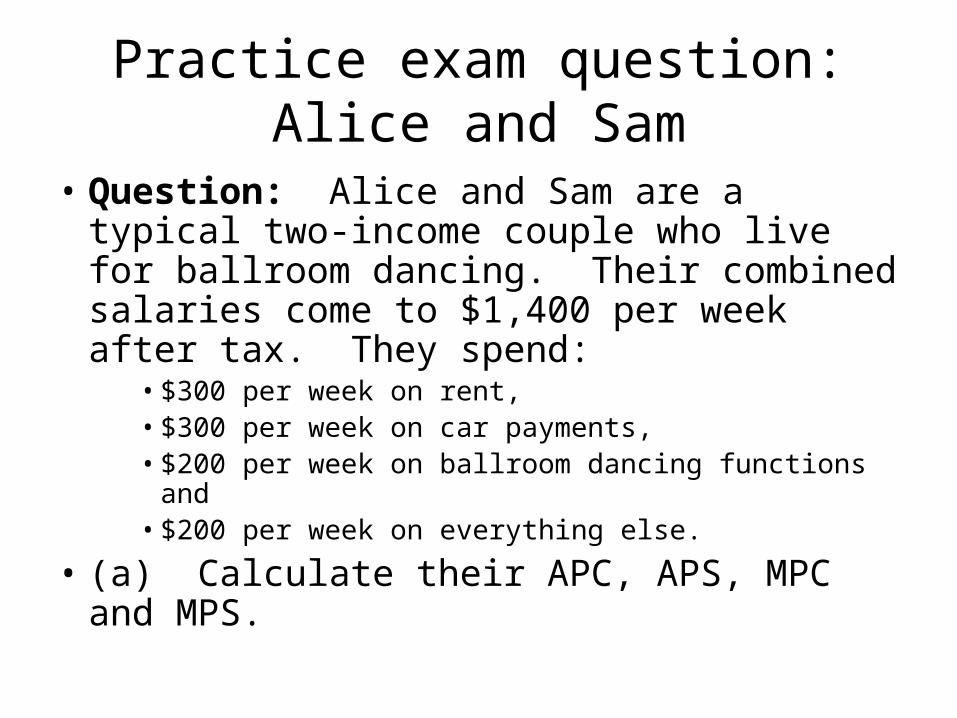
Practice exam question: Alice and Sam

• Question: Alice and Sam are a typical two-income couple who live for ballroom dancing. Their combined salaries come to $1,400 per week after tax. They spend:

• $300 per week on rent, • $300 per week on car payments, • $200 per week on ballroom dancing functions and • $200 per week on everything else.

• (a) Calculate their APC, APS, MPC and MPS.

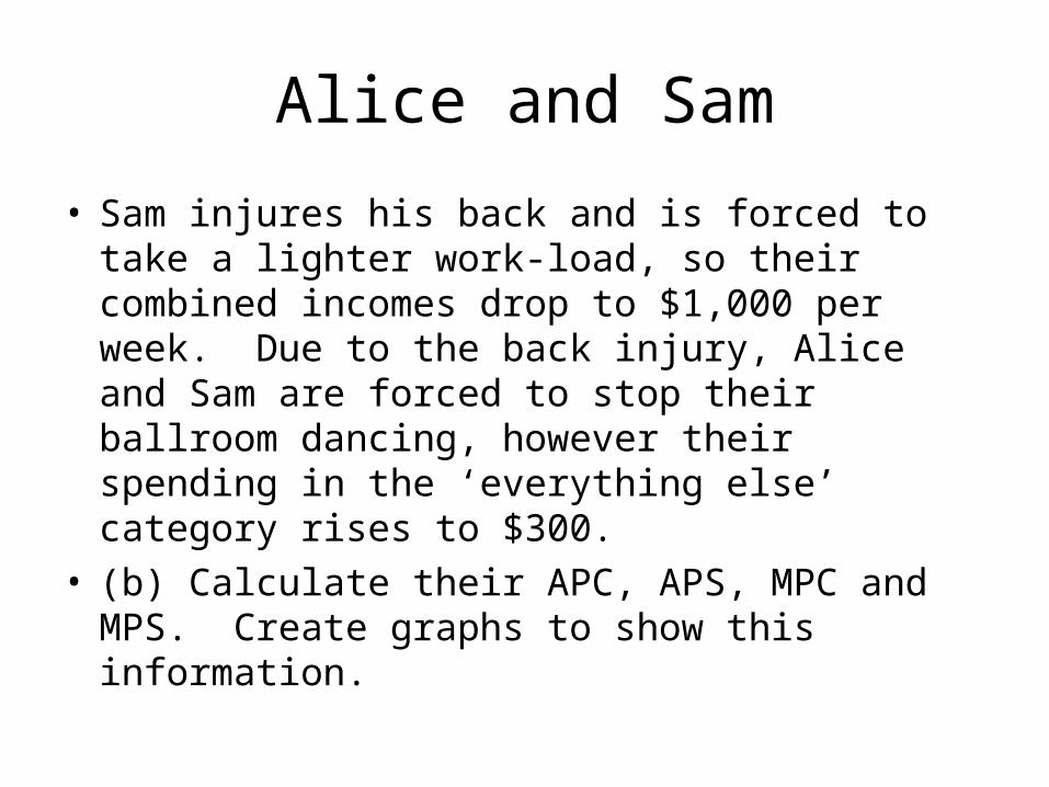
Alice and Sam

• Sam injures his back and is forced to take a lighter work-load, so their combined incomes drop to $1,000 per week. Due to the back injury, Alice and Sam are forced to stop their ballroom dancing, however their spending in the ‘everything else’ category rises to $300.

• (b) Calculate their APC, APS, MPC and MPS. Create graphs to show this information.