ECLiPSe : A Platform forConstraint Logic ProgrammingMark Wallace, Stefano Novello, Joachim SchimpfContact address: IC-Parc,William Penney Laboratory, Imperial College, LONDON SW7 2AZ.email: mgw@doc.ic.ac.ukAugust 1997AbstractThis paper introduces the Constraint Logic Programming (CLP) platform ECLiPSe .ECLiPSe is designed to be more than an implementation of CLP: it also supports math-ematical programming and stochastic programming techniques. The crucial advantage ofECLiPSe is that it enables the programmer to use a combination of algorithms appropriate tothe application at hand. This bene�t results from the ECLiPSe facility to support �ne-grainedhybridisation.ECLiPSe is designed for solving di�cult "combinatorial" industrial problems in the areasof planning, scheduling and resource allocation. The platform o�ers a conceptual modellinglanguage for specifying the problem clearly and simply, in a way that is neutral as to thealgorithm which will be used to solve it. Based on the conceptual model it is easy to constructalternative design models, also expressed in ECLiPSe . A design model is a runnable program,whose execution in ECLiPSe employs a speci�c combination of algorithms. Thus the platformsupports experimentation with di�erent hybrid algorithms.Technically the di�erent classes of algorithms mentioned above have two aspects: constrainthandling, and search. Various di�erent constraint handling facilities are available as ECLiPSelibraries. These include �nite domain propagation, interval propagation and linear constraintsolving. In ECLiPSe the same constraint can be treated concurrently by several di�erenthandlers.With regard to search behaviour, CLP and also mathematical programming typically im-pose new constraints at lower levels in the search tree. By contrast, stochastic techniquessearch for good solutions by locally repairing an original solution, and repeating the processagain and again. ECLiPSe supports both kinds of search, and allows them to be combinedinto hybrid search techniques.1 Introduction: The ECLiPSe PhilosophyThe �rst generation of constraint programming languages focussed on a single technique:constraint propagation, as described in section 4 of [Wal97]. Whilst constraint propagationhas proved itself on a variety of applications, it cannot alone su�ce to e�ciently producesolutions for typical practical industrial problems.Over the years Operations Researchers have designed highly e�cient algorithms for severalclasses of problems, such as set partitioning, matching, knapsack, and network ow problems,using techniques based on Mixed Integer Programming (MIP). More recently stochastic tech-niques, such as Simulated Annealing, have achieved striking results on optimisation problemssuch as the travelling salesman problem.1ECLiPSe is designed to take advantage of all these results, by supporting industrial scaleMIP functionality, and stochastic techniques, as well as constraint propagation and solving.1The travelling salesman problem is to �nd the shortest route which starts at a certain point, visits a given setof destinations (customers), and returns to the starting point at the end.1

More importantly, real industrial problems seldom �t into a speci�c class: the pure travel-ling salesman problem rarely comes up in real life because there are typically many salesmenavailable to cover the di�erent customers, certain customers can only be visited at certaintimes of day, also roads are busier at certain times of day so the journey time may vary withthe time of day, and anyway the poor salesmen need some time to rest - they can't usuallycomplete their circuits before lunchtime! These \side constraints" may belong to anotherproblem class - such as the class of set covering problems, or scheduling problems.Industrial problems typically have constraints that belong to di�erent problem classes -they are in a sense \hybrid". Accordingly it is not only necessary to o�er a wide choice ofalgorithms for solving such problems, but also the facility to mix and match the algorithms,i.e. to build hybrid algorithms.ECLiPSe is designed to support the fast development of speci�c hybrid algorithms tuned tothe problem at hand. It is not assumed that the �rst algorithm implemented by the applicationdeveloper is guaranteed to be the best one: rather ECLiPSe provides a platform supportingexperimentation with di�erent hybrid algorithms until an appropriate one is found which suitsthe particular features of the application.In the next section we shall explore ECLiPSe as a problem modelling language. We dis-tinguish two kinds of model: the conceptualmodel, which captures the problem speci�cation,and the designmodel, which is tuned for e�cient solving on a computer. ECLiPSe is designedto support both kinds of models, and the mapping between them.In the following two sections we shall examine the ECLiPSe facilities for handling con-straints. In [Wal97] we encountered di�erent kinds of constraints - primitive constraints,propagation constraints and constraint agents. ECLiPSe supports various classes of built-inconstraints, both primitive constraints and propagation constraints. ECLiPSe also allows com-plex constraints and constraint behaviours to be constructed from the built-in classes, thussupporting constraint agents.After constraint handling we return to the second major aspect of problem solving: thesearch for solutions.We will separate this discussion into two subsections. The �rst is concerned with con-structive search, and the second with repair-based search. Constructive search explores theconsequences of making choices for decision variables one-at-a-time. Each choice reduces theset of viable choices for the remaining decisions. By contrast repair-based search explores theconsequences, not of making decisions, but of changing them. In this case the new choice istypically compared with the previous one, in the context of other suggested choices for theother decision variables. Initially it is not expected that the suggested choices are necessarilyconsistent with the constraints. The idea of changing the choices is to reduce the number ofconstraint violations until all the constraints are �nally satis�ed.Finally there is a brief section on the ECLiPSe system, its external communication facilit-ies, embeddability, documentation and how to obtain the system.2 ECLiPSe as a Modelling Language2.1 Overview of ECLiPSe as a Modelling LanguageECLiPSe is tailored for solving combinatorial problems. Such problems are characterised by aset of decisions which have to be made (where each decision has a set of alternative choices) anda set of constraints between the decisions (so a certain choice for one decision may preclude,or entail, certain choices for other decisions).In ECLiPSe each decision is modelled by a variable, and each choice by a possible valuefor that variable. The constraints are modelled by relations between the variables. As anexample consider the map colouring program, with four countries to colour.This program was also used to illustrate constraint logic programming in [Wal97]. ECLiPSeis a constraint logic programming language, and it uses the same syntax as Prolog. Hopefullythis syntax will already be familiar to many readers. At the same time, we also hope thatany readers who have su�ered from the limitations of Prolog will not conclude that ECLiPSetherefore su�ers from the same limitations!The problem involves four decisions, one for each country. These are modelled by thevariables A, B, C and D. Countries is just a name for the list of four variables. Each2

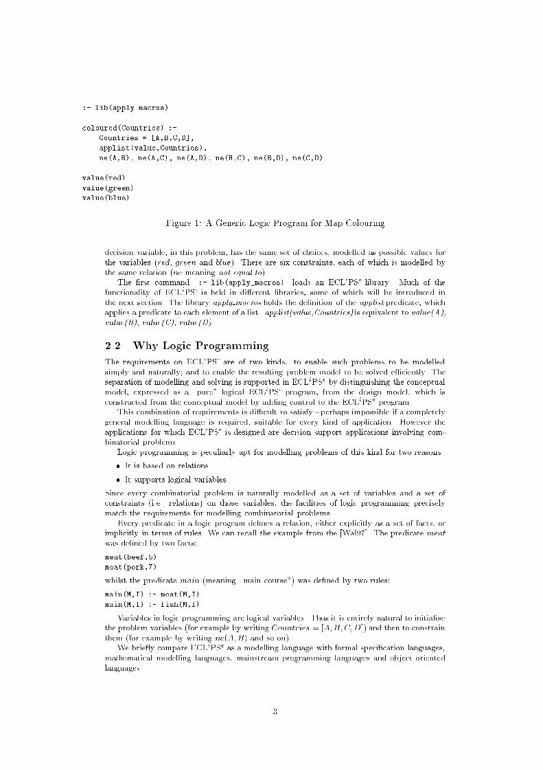
:- lib(apply_macros).coloured(Countries) :-Countries = [A,B,C,D],applist(value,Countries),ne(A,B), ne(A,C), ne(A,D), ne(B,C), ne(B,D), ne(C,D).value(red).value(green).value(blue). Figure 1: A Generic Logic Program for Map Colouringdecision variable, in this problem, has the same set of choices, modelled as possible values forthe variables (red, green and blue). There are six constraints, each of which is modelled bythe same relation (ne meaning not equal to).The �rst command :- lib(apply_macros). loads an ECLiPSe library. Much of thefunctionality of ECLiPSe is held in di�erent libraries, some of which will be introduced inthe next section. The library apply macros holds the de�nition of the applist predicate, whichapplies a predicate to each element of a list. applist(value,Countries) is equivalent to value(A),value(B), value(C), value(D).2.2 Why Logic ProgrammingThe requirements on ECLiPSe are of two kinds: to enable such problems to be modelledsimply and naturally; and to enable the resulting problem model to be solved e�ciently. Theseparation of modelling and solving is supported in ECLiPSe by distinguishing the conceptualmodel, expressed as a \pure" logical ECLiPSe program, from the design model, which isconstructed from the conceptual model by adding control to the ECLiPSe program.This combination of requirements is di�cult to satisfy - perhaps impossible if a completelygeneral modelling language is required, suitable for every kind of application. However theapplications for which ECLiPSe is designed are decision support applications involving com-binatorial problems.Logic programming is peculiarly apt for modelling problems of this kind for two reasons.� It is based on relations� It supports logical variablesSince every combinatorial problem is naturally modelled as a set of variables and a set ofconstraints (i.e. relations) on those variables, the facilities of logic programming preciselymatch the requirements for modelling combinatorial problems.Every predicate in a logic program de�nes a relation, either explicitly as a set of facts, orimplicitly in terms of rules. We can recall the example from the [Wal97]. The predicate meatwas de�ned by two facts:meat(beef,5).meat(pork,7).whilst the predicate main (meaning \main course") was de�ned by two rules:main(M,I) :- meat(M,I).main(M,I) :- fish(M,I).Variables in logic programming are logical variables. Thus it is entirely natural to initialisethe problem variables (for example by writing Countries = [A;B;C;D]) and then to constrainthem (for example by writing ne(A;B) and so on).We brie y compare ECLiPSe as a modelling language with formal speci�cation languages,mathematical modelling languages, mainstream programming languages and object orientedlanguages. 3

2.2.1 Formal Speci�cation LanguagesFormal speci�cation language are designed for formality, but not for execution. Consequentlythey include constructs, such as universal quanti�cation, which are precisely de�ned but arenot constructive. In other words there are constructs which cannot be mapped onto any(practical) algorithm.Luckily the class of problems for which ECLiPSe is designed have a �nite set of decisionvariables each of which admits only �nitely many alternatives. Consequently it is only ne-cessary to support a restricted form of logic2 which is easier to understand and easier toimplement. The nearest thing ECLiPSe o�ers to universal quanti�cation is iteration over�nite sets, as for example the goal applist(value,Countries) in �gure 1.The restricted logic of ECLiPSe has a bene�t that the mapping from the conceptual modelof the problem to the design model is an extension of the conceptual model rather than arewriting. This means that when problem requirements change it is natural to capture thischange in the conceptual model, and then carry them through to the design model. The resultis that during application development the conceptual model and the design model remain instep. This avoids many of the pitfalls which await developers working on applications whosespeci�cations are changing even during application development!2.2.2 Mathematical Modelling LanguagesThere already exists a class of modelling languages designed for combinatorial problems.These are the mathematical modelling languages typically used as input to mixed integerprogramming (MIP) packages. We further discuss MIP, and how to use it through ECLiPSe, in section 3.4 below.Although the syntax is di�erent, mathematical modelling languages share many of thefeatures of logic programming. They support logical variables, and constraints. They supportnumerical constraints which, though not supported in traditional logic programs, are supportedby constraint logic programs as we shall see in the following section. They support namedconstraints, which is achieved in constraint logic programming by introducing a predicatename, eg precede(T1,T2) :- T1 >= T2.There are two facilities in constraint logic programming which are not available in math-ematical modelling languages. The main one is quite simple: in constraint logic programs itis possible to de�ne a constraint which involves a disjunction. Mathematical programmingcannot handle disjunction directly. The second di�erence is that logic programming allowsnew constraints to be de�ned in terms of existing ones, even recursively. In mathematical pro-gramming the model is essentially at, which not only complicates the model but also reducesreuseability within an application and across applications.To illustrate the advantage of handling disjunction in the modelling language, we take atoy example and present two models: a mathematical programming model and a constraintlogic programming model.Consider the constraint that two tasks sharing a single resource cannot be done at thesame time. The constraint involves six variables: the start times S1; S2, end times E1; E2 andresources R1; R2 of the two tasks. The speci�cation of this constraint is as follows:either the two tasks use distinct resource ( R1 ne R2) or task1 ends beforetask2 starts (E1 � S2) or else task2 ends before task1 starts (E2 � S1).First we shall show how it can expressed as a mathematical model without disjunctions. Forthis purpose it must be encoded using numerical equations and inequalities, together withinteger constraints.The disjunctions can be captured by introducing three 0/1 variables, Br1, Br2, and Bt,and using some large constant, say 100000, larger than any possible values for any of the sixvariables. Now we can express the constraint in terms of numerical inequalities as follows:R1 + 100000 �Br1 + 100000 �Br2 � R2 + 1R2 + 100000 � Br1 + 100000 � (1� Br2) � R1 + 1S1 + 100000 � (1�Br1) + 100000 � Bt � E2S2 + 100000 � (1�Br1) + 100000 � (1�Bt) � E12technically called Horn clauses 4

If Br1 = 0 then the two tasks use di�erent resources. In this case, if also Br2 = 0 thenR1 � R2 + 1, otherwise Br2 = 1 and R2 � R1 + 1. It is an exercise for the reader to provethat if Br1 = 0 then the tasks can overlap. Otherwise, if Br1 = 1, then Bt = 0 entails S1 � E2and Bt = 1 entails S2 � E1.In ECLiPSe this constraint can be modelled directly in logic, as illustrated in �gure 2.taskResource(S1,E1,R1,S2,E2,R2) :-ne(R1,R2).taskResource(S1,E1,R1,S2,E2,R2) :-R1=R2, S1 >= E2.taskResource(S1,E1,R1,S2,E2,R2) :-R1=R2, S2 >= E1.Figure 2: Specifying a Resource Contention Constraint in ECLiPSeWe note that the ECLiPSe model is a conceptual model, whilst the mathematical modelis a design model. The point here is that in ECLiPSe both models can be expressed, whilstmathematical modelling can only express a design model. Indeed we shall show in section 4.1below a design model written in ECLiPSe that is very close to the conceptual model.Another ECLiPSe design model, which is also close to the conceptual model, is handledin ECLiPSe by an automatic translator which builds the MIP model and passes it to theMIP solver of ECLiPSe . This translator is described in [RWH97] which is available from theIC-Parc home page (whose URL is given in section 6 below).Whilst the above example shows that such complex constraints can be expressed in terms ofnumerical inequalities, as required for MIP, the encoding is awkward and di�cult to debug. Itbecomes increasingly di�cult as the constraints become more complex (eg the current exampleimmediately becomes harder still if the resources have a �nite capacity greater than one).Notice, �nally, that the mathematical model requires resources to be identi�ed by numbers,whilst the constraint logic programming model imposes no such restriction as we shall showin section 4 below.2.2.3 Mainstream Programming LanguagesNaturally the implemented solution to an industrial problem must be delivered into the indus-trial computing environment. It is sometimes argued that this is only possible if the solutionis implemented in a mainstream programming language such as C, C++ or even Java. Thereare two arguments supporting this view, �rstly that of embeddability (it is easier and more ef-�cient to pass data and control between modules written in the same programming language),and secondly that of system support (mainstream language programmers are much easier to�nd and replace than specialist programmers).Whilst this argument only supports a mainstream programming language being used forimplementation, and not conceptual modelling, it has consequence for the modelling languageas well on the assumption, which we discussed above, that the conceptual model should beclose to the design model. Thus if the design model is encoded in a mainstream programminglanguage, then either the conceptual model must be compromised becoming more like a designmodel, or the gap between the conceptual model and design model grows very wide.Sadly the attempt to tackle combinatorial problems with mainstream programming lan-guages has too often foundered because the implemented solution has proved not to solve theactual industrial requirement (often because requirements change during application develop-ment). The solution cannot then be modi�ed to meet the actual, or new, requirements withina reasonable cost and timescale.Given that the core combinatorial optimisation problem is best solved by a specialisedprogramming platform (either mathematical or constraint-based), the problem of embeddinghas to be solved.One approach is to embed constraint solving in a mainstream programming language. Aswe shall see in section 5 below, search and constraint handling are closely interdependent.Even if the search is encoded in a mainstream programming language, the programmer is5

required to understand in detail not only the data structures used by the constraint handlers,but their operational behaviour.In practice packages providing an embedding of constraints in mainstream programminglanguages also encapsulate search within the package. The application developer is requiredto control the search. To avoid any mismatch between the host programming language andsearch control within the package, a popular approach is to implement the package as a libraryof the host programming language.The result is that the separation of conceptual modelling and design modelling is given up,in favour of staying within the con�nes of the expressive capabilities of the host programminglanguage. This approach not only requires specialist programmers to develop and supportthe application, but it also sacri�ces the modelling advantages of mathematical and constraintlogic programming.In fact the problem of embedding has been overcome, though �rst generation constraintlogic programming languages were de�cient in this area. ECLiPSe is fully embeddable in Cand C++, and indeed uses an external solver, written in C to handle linear constraints, since theruntime cost of such an interface is perfectly acceptable even for a tightly integrated componentsuch as a constraint handler!2.2.4 Object Oriented LanguagesECLiPSe supports object-orientation through two distinct features, modules and structures.Modules support behavioural object orientation, and structures support structural object ori-entation.Because of the nature of combinatorial problems, the only requirement for behaviouralobject orientation is in the constraint handlers. The implementation of each constraints libraryis hidden inside a module, and access to the internal data structures is only through predicatesexported from the module.The remaining objects that can occur in an ECLiPSe model have attributes but no beha-viour, and so they require only structural object orientation.In our �rst example we modelled a map colouring problem using only variables and con-straints. It can be argued, however, that for more complex applications, the conceptual modelcan bene�t from a notion of object, into which variables can be built. For example in mod-elling a resource scheduling problem the notion of a task with certain attributes is useful. Atask might have an identi�er, a start time, and end time and a duration.After declaring structures for tasks and times, as in �gure 3, the programmer can accessany of their attributes independently.[eclipse 1]: lib(structures).* structures loaded[eclipse 2]: define_struct( task(id, start, end, duration)),define_struct( time(hour, minute)).* yes.[eclipse 3]: T=task with [id:a,duration:10].* T = task(a, _, _, 10)* yes.[eclipse 4]: T1=task with [id:a3,start:S3,end:(time with hour:H3)],T2=task with [id:a4,start:S3,end:(time with hour:H4)],H3>H4.* T1 = task(a3, S3, time(H3, _), _)* T2 = task(a4, S3, time(H4, _), _)* yes. Figure 3: De�ning a Task Structure6

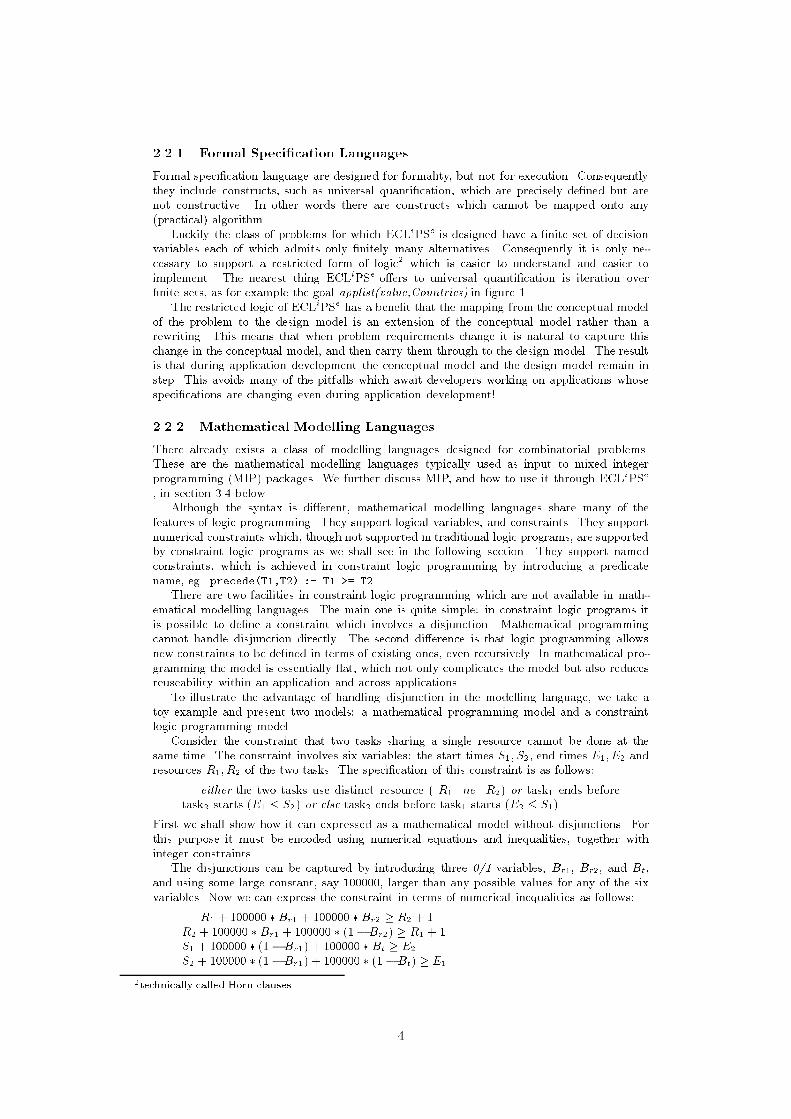
Each ECLiPSe prompt (eg [eclipse 1]:) is followed by a user query (eg lib(structures).).In the rest of the article, \query N" always refers to the query which is preceded by the prompt[eclipse N]:.The programmer enters lib(structures). to which the system responds structures loaded.I have added a star to the beginning of each line showing a system response.Query 2 de�nes the attributes for objects in the classes task and time. Query 3 shows howthe user can equate a variable with a structured object (i.e. the variable is instantiated to thestructure). ECLiPSe automatically constructs unknown values (written _) for the unspeci�edattributes.Query 4 illustrates something of the expressive power needed in a constraint programminglanguage which supports objects. Not only do the objects T1 and T2 share an attributevalue - this is a shared subobject - but they also have non-shared subobjects whose attributesare connected by a constraint. Such a constraint, between distinct objects, is typically notexpressible within the traditional object-oriented framework.2.3 The Conceptual Model and the Design ModelThe main bene�t of constraint logic programming over other platforms for solving combinator-ial problems is in the closeness between the conceptual model and the design model. ECLiPSetakes full advantage of this by o�ering facilities to choose di�erent annotations of the same con-ceptual model to achieve design models which, whilst syntactically similar, can have radicallydi�erent behaviour.2.3.1 Map ColouringLet us start by mapping the conceptual model for the map colouring example illustrated in�gure 1 into a design model which uses the �nite domain constraint handler of ECLiPSe .The design model is encoded as shown in �gure 4.:- lib(fd).coloured(Countries) :-Countries=[A,B,C,D],Countries :: [red,green,blue],ne(A,B), ne(A,C), ne(A,D), ne(B,C), ne(B,D), ne(C,D),labeling(Countries).ne(X,Y) :- X##Y. Figure 4: A Finite Domain CLP Program for Map ColouringThe design model extends the conceptual model in four ways.1. The ECLiPSe �nite domain library is loaded (using :- lib(fd)).2. An explicit �nite domain is associated with each decision variable (using Countries ::[red, green, blue]).3. The �nite domain built-in disequality constraint is used to implement the ne constraint(using ne(X,Y) :- X##Y). ## is a special syntax for disequality used by the �nite domainconstraint solver.4. This program includes a search algorithm, invoked by the goal labeling(Countries). Aswe shall see later, this predicate tries choosing, for each of the variables A, B, C andD in turn, a value from its domain. It succeeds when a combination of values has beenfound that satis�es the constraints.Naturally this is a toy example, and it is not always so easy to turn a conceptual model,such as the ECLiPSe program in �gure 1, into a design model, such as the program in �gure4. Nevertheless constraint logic programming, and in particular ECLiPSe , have made a lot of7

progress in achieving a close relationship between the conceptual model and the design model.The di�erent components of the ECLiPSe system all support the separate development ofa clear, correct conceptual model, and an e�cient design model, and they also support themapping between the two.2.3.2 Having Enough Change in Your PocketLet us now take a more interesting problem, which has been set as a recent challenge withinthe MIP community. The problem is apparently rather simple: what is the minimum numberof coins a purchaser needs in their pocket in order to be able to buy any one item costing lessthan one pound, and guarantee to be able to pay the exact amount?The problem involves only six decision variables, one for the number of coins of eachdenomination held in the pocket (the denominations are 1,2,5,10,20,50).The conceptual model for this problem is shown in �gure 5.:- lib(apply_macros).solve(PocketCoins,Min) :-PocketCoins=[P,Tw,Fv,Te,Twe,Ff], %1applist(range(0,99),[Min|PocketCoins]), %2Min = P+Tw+Fv+Te+Twe+Ff, %3fromto(1,99,genc(PocketCoins)), %4minimize(Min). %5genc(PocketCoins,Total) :-Coins=[P1,Tw1,Fv1,Te1,Twe1,Ff1], %6applist(range(0,99),Coins), %7Total = P1+2*Tw1+5*Fv1+10*Te1+20*Twe1+50*Ff1, %8maplist( '<=',Coins,PocketCoins). %9Figure 5: Conceptual Model for the Coins ProblemThe lines are numbered, using the syntax %N, as % is a comment symbol in ECLiPSe . Wedescribe this program line by line.1. The variable PocketCoins is just a shorthand for the list of six variables, [P, Tw, Fv, Te,Twe, Ff] which denote the number of coins of each denomination held in the pocket.2. [A,B,C] is a list, but ECLiPSe allows lists to be written in an alternative syntax [Head| Tail]. Thus [Min | PocketCoins] is simply another way of writing the list of sevenvariables, [Min, P, Tw, Fv, Te, Twe, Ff]. The command applist(range(0,99), [Min |PocketCoins]) associates a range (between 0 and 99) with each of the variables.3. Min is the total number of coins in the pocket, as enforced by the equation Min =P+Tw+Fv+Te+Twe+Ff.4. To ensure that these coins are enough to make up any total between 1 and 99, we nowimpose 99 further constraints, one for each total. genc(PocketCoins,Total) is called foreach value of Total between 1 and 99.5. minimize(Min) simply speci�es that the best feasible solution to the problem is one whichminimises the value of the variable Min.6. genc(PocketCoins,Total) initialises another set of coins [P1, Tw1, Fv1, Te1, Twe1, Ff1]needed to make up the total Total.7. This set of coins is also initialised to range between 0 and 998. Their total value is constrained to be equal to Total. This constraint is enforced by theequation Total = P1+ 2*Tw1 + 5*Fv1 + 10*Te1 + 20*Twe1 + 50*Ff1.8

9. Finally the constraint that the required coins of each denomination must be less than,or equal to, the number of coins of that denomination in the pocket, is enforced by theconstraints: P1 <= P, Tw1 <= Tw, Fv1 <= Fv, Te1 <= Te, Twe1 <= Twe, Ff1 <= Ff.These constraints are generated by the single command maplist( <=, Coins, Pocket-Coins).Let's start by trying mixed integer programming on this problem. To do this we addinteger declarations for each of the integer variables, and change the constraints to use thesyntax recognised by the (external) MIP solver accessed via the ECLiPSe library eplex. Forequations we use the syntax $=, and for inequalities we use $>=. The design model is shownin �gure 6.:- lib(apply_macros).:- lib(eplex).solve(PocketCoins,Cost) :-PocketCoins=[P,Tw,Fv,Te,Twe,Ff],applist(range(0,99),[Min|PocketCoins]),Min $= P+Tw+Fv+Te+Twe+Ff,fromto(1,99,genc(PocketCoins)),optimize(min(Min),Cost).genc(PocketCoins,Total) :-Coins=[P1,Tw1,Fv1,Te1,Twe1,Ff1],applist(range(0,99),Coins),Total $= P1+2*Tw1+5*Fv1+10*Te1+20*Twe1+50*Ff1,maplist( '$=<',Coins,PocketCoins).range(Min,Max,Var) :-integers(Var),Var $>= Min,Var $=< Max. Figure 6: Conceptual Model for the Coins ProblemThis program passes all the $= and $>= constraints to the CPLEX mixed integer program-ming package [CPL93], and invokes the CPLEX branch and bound solver, to minimise thevalue of the variable Min. This minimum is placed in the variable Cost.As such this model can only solve the problem of producing the exact change up to 59pence (replacing 99 with 59 in the above program). For the full problem the system runs outof memory. There are standard MIP solutions to the problem which run overnight, but it is atough challenge to reduce this time from hours to minutes!In �gure 7 we illustrate an ECLiPSe program for solving the \Coins" problem using thefacilities of the ECLiPSe �nite domain constraint solver implemented in the ECLiPSe libraryfd. In this case the #= and #>= constraints and the optimisation predicate minimize are imple-mented in the ECLiPSe �nite domain library. This program proves within a few seconds thatthe minimum number of coins a purchaser needs in their pocket to make up any total between1 and 99 is eight coins! One solution is: P = 1; Tw = 2; Fv = 1; Te = 1; Twe = 2; Ff = 1.We have shown how the same underlying model for the \Coins" problem can be passed todi�erent solvers so as to use the best one. However in ECLiPSe it is not a choice of either/or:the same constraints can easily be passed to several solvers at the same time! For instance wecan de�ne X $#= Y to be both X $= Y and X #= Y and replace = in the above model with $#=,and we can treat >= similarly.Whilst for this problem the �nite domain solver alone solves the problem most e�ciently,we have encountered practical examples where the combination of both solvers outperformseach on its own. 9

:- lib(apply_macros).:- lib(fd).solve(PocketCoins,Min) :-PocketCoins=[P,Tw,Fv,Te,Twe,Ff],applist(range(0,99),[Min|PocketCoins]),Min #= P+Tw+Fv+Te+Twe+Ff,fromto(1,99,genc(PocketCoins)),minimize(labeling(PocketCoins),Min).genc(PocketCoins,Total) :-Coins=[P1,Tw1,Fv1,Te1,Twe1,Ff1],applist(range(0,99),Coins),Total #= P1+2*Tw1+5*Fv1+10*Te1+20*Twe1+50*Ff1,maplist( '#<=',Coins,PocketCoins).range(Min,Max,Var) :-Var::Min..Max Figure 7: fd Constraints for the Coins Problem3 Solvers and SyntaxECLiPSe o�ers several di�erent libraries for handling symbolic and numeric constraints. Theyare the fd (�nite domain) library, the range library, the ria (real number interval) library, and�nally the eplex (MIP) library.3.1 The fd (Finite Domain) LibraryThe �nite domain library has been used and re�ned over a 10 year period. As a result it hasa great many constraint handling facilities. It is best seen as three libraries.The �rst is a library for handling symbolic �nite domains, with values like red, machine 1etc. The built-in constraints on symbolic �nite domain variables are equations and disequalit-ies: these constraints can only hold between expressions which are either constants or variables.These constraints can also be used when the domains are numeric.The second is a library for handling integer variables, and numerical constraints on thosevariables. The library propagates equations and inequalities between linear expressions. Alinear numeric expression is one that can be written in the form Term1+Term2+: : :+Termn,where each term can, in turn, be written Number or Number � V ariable. The number canbe positive or negative. An example is the expression 3 �X + (�4) � Y + 3 (which we wouldnormally write 3 �X � 4 � Y + 3).The third is a library supporting some built-in complex constraints. Two examples of suchconstraints are the alldistinct constraint, which constraints a set of variables to take valueswhich are pairwise distinct, and the atmost constraint, which constrains at most N variablesfrom a given set to take a certain value.3.1.1 The fd Symbolic Finite Domain FacilitiesIn �gures 1 and 4, above, we showed a map colouring problem and its solution. The domainsassociated with the countries were red, green and blue. These were declared as �nite domains,with the usual syntax: X :: [red, green, blue].The problem could have been modelled using numbers to represent colours, so there isno extra power in allowing symbolic �nite domains as well as numeric ones. However whendeveloping ECLiPSe programs for real problems, it is a very great help to use meaningfulnames so as to distinguish di�erent types of �nite domain variables. In particular it is crucialduring debugging! 10

Figure 8 illustrates the basic constraints on �nite domain variables, and predicates foraccessing and searching these domains.The second query associates a symbolic �nite domain with the variable X. In responseECLiPSe prints out the variable name and its newly assigned domain. The fact that thevariable has an associated domain does not require any changes in other parts of the program,where X may be treated as an ordinary variable.Query 3 shows that symbolic domains can include values of di�erent types.Query 4 shows the use of the dom predicate to retrieve the domain associated with avariable.Queries 5 and 6 illustrate the equality and disequality constraints, and their e�ects on thedomains of the variables involved. Finite domain constraints use a special syntax to makeexplicit which constraint library is to handle the constraint, for example it uses #= instead of=. Queries 7, 8 and 9 illustrate search. Strictly one would not expect search predicatesto belong to a constraint library, but in fact search and constraint propagation are closelyconnected.Query 7 shows the indomain predicate instantiating a domain variable X to a value inits domain. ECLiPSe asks if more answers are required, and when the user does indeed askfor more, another value from the domain of X is chosen, and X is instantiated to that valueinstead. When the user asks for more again, X is instantiated to the third and last value in itsdomain, and this time ECLiPSe doesn't o�er the user any further choices, but simply outputsyes.Query 8 illustrates the built-in �nite domain labeling predicate. This predicate simplyinvokes indomain on each variable in turn in its argument. In this case it calls indomain �rston X, then Y and then Z. However the variables are constrained to take di�erent values bythree disequality constraints, and only those labelings that satisfy the constraints are admitted.Consequently this query has six di�erent answers, though the user stops asking for more afterthe second answer.Query 9 illustrates a heuristic based on the fail �rst principle. In choosing the nextdecision to make, when solving a problem, it is often best to make the choice with the fewestalternatives �rst. The predicate delete� selects a variable from a set of variables which has thefewest alternatives: i.e. the smallest �nite domain. In the example there are three variables, X,Y and Z representing three decisions, delete� picks out Y because it has the smallest domain,and then indomain selects a value for Y . The third argument of delete� is an output argument:Rest returns the remaining variables after the selected one has been removed. These are thedecisions yet to be made.3.1.2 The fd Integer Arithmetic FacilitiesFor numeric �nite domains the fd library admits equations, inequalities and disequalities overnumeric expressions.Additionally the fd library includes some built-in optimisation predicates. These are allillustrated in �gure 9.Query 2 illustrates how a numeric �nite domain can be initialised just by giving lower andupper bounds, instead of the whole list of members. In fact, internally, �nite domains arestored as lists of intervals (for example [1..5, 8..10, 15]).Query 3 shows how the user can �nd out the lower bound of a variable's numeric �nitedomain. There is a similar predicate for retrieving the upper bound.Queries 4, 5 and 6 illustrate some features of �nite domain constraint propagation.Query 4 shows the pruning achieved by a simple numerical �nite domain constraint. Noticethat both the domains of X and Y are pruned - constraints work in all directions!Query 5 illustrates that a �nite domain constraint remains active even after it has achievedsome pruning. This query is the same as query 3, with an extra constraint imposed sub-sequently. The X# > Y +1 constraint is still active, and prunes the domain of X still furtherfrom [3..10] to [8..10].Query 6 shows that, in the interest of computational e�ciency, the mathematical constraintsonly narrow the bounds of the �nite domains. In this example the domain of X could theor-etically be reduced to [4,6,8,10], but this would require much more computation - especiallyif the �nite domains were quite large! 11

[eclipse 1]: lib(fd).* fd loaded[eclipse 2]: X::[a,b,c].* X = X{[a, b, c]}* yes.[eclipse 3]: X::[a, 3.1, 7].* X = X{[3.0999999, 7, a]}* yes.[eclipse 4]: X::[a,b,c], dom(X,List).* X = X{[a, b, c]}* List = [a, b, c]* yes.[eclipse 5]: X::[a,b,c], Y::[b,c,d], X#=Y.* X = X{[b, c]}* Y = X{[b, c]}* yes.[eclipse 6]: X::[a,b,c], X##b.* X = X{[a, c]}* yes.[eclipse 7]: X::[a,b,c], indomain(X).* X = a More? (;)* X = b More? (;)* X = c* yes.[eclipse 8]: [X,Y,Z]::[a,b,c], X##Y, Y##Z, X##Z, labeling([X,Y,Z]).* X = a* Y = b* Z = c More? (;)* X = a* Y = c* Z = b More? (;)* yes.[eclipse 9]: [X,Z]::[a,b,c], Y::[a,c],deleteff(Var,[X,Y,Z],Rest), indomain(Var).* X = X{[a, b, c]}* Y = a* Z = Z{[a, b, c]}* Rest = [X{[a, b, c]}, Z{[a, b, c]}]* Var = a More? (;)* yes. Figure 8: Using Symbolic Finite Domains12

[eclipse 1]: lib(fd).* fd loaded[eclipse 2]: X::1..10.* X = X{[1..10]}* yes.[eclipse 3]: X::1..10, mindomain(X,Min).* X = X{[1..10]}* Min = 1* yes.[eclipse 4]: [X,Y]::1..10, X#>Y+1.* X = X{[3..10]}* Y = Y{[1..8]}* yes.[eclipse 5]: [X,Y]::1..10, X#>Y+1, Y#=6.* X = X{[8..10]}* Y = 6* yes.[eclipse 6]: [X,Y,Z]::1..10, X #= 2*(Y+Z).* X = X{[4..10]}* Y = Y{[1..4]}* Z = Z{[1..4]}* yes.[eclipse 7]: X::1..10, mindomain(X,Min).* X = X{[1..10]}* Min = 1* yes.[eclipse 8]: [X,Y,Z]::1..10, X #= 2*(Y+Z), Y##Z,minimize(labeling([X,Y,Z]),X).* Found a solution with cost 6* Y = 2* Z = 1* X = 6* yes. Figure 9: Numeric Finite Domains13

Query 7 is an example of the use of the built-in minimize predicate. This predicate returnsan admissible labeling of the variables X, Y and Z which yields the smallest value for X.In general any search procedure can be substituted for labeling([X,Y,Z]) as the �rst argu-ment to minimize. For example we could have used minimize( (indomain(X), indomain(Y),indomain(Z)), X).3.1.3 The fd Complex ConstraintsThere are two motivations for supporting complex constraints. One is to simplify problemmodelling. It is shorter, and more natural, to use a single alldistinct constraint on N variablesthan to use n � (n� 1)=2 (pairwise) disequalities!The second motivation is to achieve specialised constraint propagation behaviour. Thealldistinct constraint on N variables, has the same semantics as n � (n � 1)=2 (pairwise)disequalities, but it can also achieve better propagation than would be possible with thedisequalities. For example if any M of the variables have the same domain, and its size is lessthan M , then the alldistinct constraint can immediately fail. However if two variables Xand Y have the same domain, with M > 1 elements, the constraint X ## Y can achieve nopropagation at all. Thus the pairwise disequalities are unable to achieve the same propagationas the alldistinct constraint.The constraint atmost(Number;List; V al) constrains atmost Number of the variables inthe list List to take the value V al. This is a di�cult constraint to express using logic. Oneway is to constrain each sublist of length Number+1 to contain a variable with value di�erentfrom V al, but the resulting number of constraints can be very large!A more natural way is to constrain all the variables to take a value di�erent from V al, andto allow the constraint to be violated up to N times. The fd library supports such a facilitywith the constraint #=(T1, T2, B). This constraint makes B = 1 if T1 = T2 and B = 0otherwise. It is possible to express atmost by imposing the constraint # = (V ari; V al; Bi)for each variable V ari in the list and then adding the constraint B1 + : : :+Bm# <= N . Thebuilt-in atmost constraint is essentially implemented like this.The other fd constraints (#<, #>, etc.) can be extended with an extra 0/1 variable in thesame way.The fd library includes a great variety of facilities, which are best explored by obtaining theECLiPSe extensions manual [Be97] and looking at the programming examples in the sectionon the fd library there.3.2 The range LibraryThe range library does very little itself, but it provides a common basis for the interval andthe MIP libraries. By contrast with the �nite domain library, the range library admits rangeswhose lower and upper bound are either real numbers or integers. The library enables theprogrammer to associate a range with one or more variables, as illustrated in �gure 10.[eclipse 1]: lib(range).* range loaded[eclipse 2]: X::0.0..9.5, lwb(X,4.5).* X = X{4.5 .. 9.5}* yes.[eclipse 3]: X::4.5..9.5, X=6.0.* X = 6.0* yes.[eclipse 4]: X::4.5..9.5, X=1.0.* no (more) solution.[eclipse 5]: X::0.0..9.5, lwb(X,4.5), integers([X]).* X = X{5 .. 9}* yes. Figure 10: Example Queries Using the range Library14

In query 2, the programmer enters X::0.0..9.5, lwb(X,4.5)., and the system respondsby printing out the resulting range. When the variable is instantiated, the range is checked forcompatibility, as shown by queries 3 and 4.Finally, what might be treated as type information in other programming paradigms, canbe treated as a constraint in the constraint programming paradigm. Thus we can add aconstraint that something is an integer in the middle of a program, as shown by query 5.3.3 The ria (Real Interval Arithmetic) LibraryThe ria library supports numeric constraints which may involve several variables. Throughoutprogram execution, ria continually narrows the ranges associated with the variables as far aspossible based on these constraints. In other words ria supports propagation of intervals,using the range library to record the current ranges, and to detect inconsistencies.The constraints handled by ria are equations and inequalities between numerical expres-sions. The expressions can be quite complex, they can include polynomials and trigonomet-rical functions. This functionality is quite similar to that o�ered by fd, except that fd canonly propagate linear constraints. On the other hand, the �nite domain library uses integerarithmetic instead of real number arithmetic, so it is in general more e�cient than ria.We shall con�ne ourselves here to a single example showing ria at work.Suppose we wish to build a garden house, whose corners must lie on a given circle. Thehouse should be a regular polygon, but may have any number of sides. It should be as large aspossible within these limitations. (Note that the more sides the larger the area covered, untilit covers practically the whole of the circle.) However each extra side incurs a �xed cost. Theproblem is to decide how many sides the garden house should have?If it had six sides, the house would look as illustrated in �gure 11.Rad Y

X Figure 11: The Garden HouseThe area of the house is 2*6*A where A is the area of the triangle in the illustration. Thearea of an N-sided house can be modelled in ECLiPSe as shown in �gure 12. N is the numberof sides, and Area is the area of the house. The variable Rad denotes the radius of the circle,and X and Y are the lengths of the sides of the triangle, as illustrated in �gure 11.ria requires its constraints to be written with a speci�c syntax (eg X *>= Y instead of justX >= Y). This distinguishes ria constraints from linear and �nite domain constraints, whicheach have their own special syntax.To work out the payo� between the area and the number of sides, we de�ne the cost of thehouse to be W1 �Area�W2 �N , where W1 and W2 are weighting factors that we can choseto re ect the relative costs and bene�ts of the area against the number of sides. In the modelshown in �gure 12, tcost returns the cost-bene�t of an N-sided house in case the radius of thecircle is 10, and the weights are W1 = 1 and W2 = 10.We can place this program in a �le called house.pl, and then use ECLiPSe to �nd out somecosts by �rst \consulting" the �le, as illustrated �gure 13, query 1.Queries 2-6, in �gure 13, would seem to indicate that the seven sided house is best for thegiven cost weightings.3However it is also interesting to see whether the interval reasoning system itself can achieveuseful propagation without even knowing the number of sides of the house. We show this inquery 7.3The intervals returned from ria are much narrower than this, but for this paper I have reduced the output tothree signi�cant �gures. 15

:- lib(ria).area(N,Rad,Area) :-X*>=0, Y*>=0, N*>=3, integers(N),Rad *>=0, Area*>=0,Area *=< pi*sqr(Rad),cos(pi/N) *= Y/Rad,sqr(Y)+sqr(X) *= sqr(Rad),Area *= N*X*Y.cost(N,Rad,W1,W2,Cost) :-W1*>=1, W2*>=1, Cost *>=0,area(N,Rad,Area),Cost *= W1*Area-W2*N.tcost(N,Cost) :-cost(N,10,1,10,Cost).Figure 12: The Area, and Cost-Bene�t, of a Garden House[eclipse 1]: [house].* range loaded* house.pl compiled* yes.[eclipse 2]: tcost(3,C).* C = C{99.90 .. 99.91}* yes.[eclipse 3]: tcost(4,C).* C = C{159.9 .. 160.0}* yes[eclipse 4]: tcost(6,C).* C = C{199.8 .. 199.9}* yes.[eclipse 5]: tcost(7,C).* C = C{203.6 .. 203.7}* yes.[eclipse 6]: tcost(8, C).* C = C{202.8 .. 202.9}* yes.[eclipse 7]: tcost(N,C).* N = N{3 .. 31}* C = C{0.0 .. 284.2}* yes.[eclipse 8]: tcost(N,C), squash([C],1e-2,lin).* N = N{3 .. 31}* C = C{0.0 .. 224.2}Figure 13: Finding the Optimal Shape for a Garden House16

An upper bound on the number of sides is extracted due to the constraint that the cost-bene�t must be positive, but the propagation on the cost-bene�t is rather weak. In cases likethis, propagation can be augmented by a technique known as squashing, as illustrated in query8. We now give two short examples showing limitations of interval reasoning in general. Thiswill motivate the introduction of a linear constraint solver in ECLiPSe , described in section3.4.The two limitations are that interval reasoning cannot, even in some quite simple examples,detect inconsistency among the constraints; and in cases where the constraints have only onesolution, interval reasoning often fails to re ect this in the results of propagation.This is illustrated by a couple of simple examples in �gure 14. In this case the system[eclipse 1]: lib(ria).* ria loaded[eclipse 2]: [X,Y,Z]:: -100.0..100.0,X+Y *=<1, Z+X*=<1, Y+Z*=<1, X+Y+Z*>=2.* X = X{-100.1 .. 100.1}* Y = Y{-100.1 .. 100.1}* Z = Z{-100.1 .. 100.1}* yes[eclipse 3]: [X,Y]:: -100.0 .. 100.0, X+Y *= 2, X-Y *= 0.* X = X{-98.1 .. 100.1}* Y = Y{-98.1 .. 100.1}* yes Figure 14: Poor Interval Propagation Behaviourfailed to detect the inconsistency in query 2, and did not deduce that only one value waspossible for X and Y in query 3. The answer is not incorrect, as ria only guarantees thatany possible answers must lie in the intervals returned - it does not guarantee the existence ofan answer in that interval. Nevertheless it would be useful to have available a more powerfulsolver to recognise cases such as these.3.4 The eplex (External CPLEX Solver Interface) LibraryEquations and inequalities between linear numeric expressions, as de�ned in section 3.1 above,are a subset of the constraints which can be handled by ria. However this class can be handledvery powerfully, so much so that any inconsistency between the constraints is guaranteed tobe detected. Techniques for solving linear constraints have been at the heart of operationsresearch for half a century, and highly e�cient linear solvers have been developed.One of the most widely distributed, scaleable and e�cient packages incorporating a lin-ear constraint solver is the CPLEX MIP package [CPL93]. CPLEX o�ers several algorithmsfor solving linear constraints including the Simplex and Dual Simplex algorithms. These al-gorithms are supported by sophisticated data structures, and the package can handle problemsinvolving ten of thousands of linear constraints over ten of thousands of variables.In the discussion so far, we have not yet mentioned an important aspect of most industrialcombinatorial problems. Not only is it required to make decisions that satisfy the constraints,but they must also be chosen to optimise some measure. In the travelling salesman problemfor example, the decisions of what order to visit the cities are based on optimising the totaldistance travelled by the salesman.One feature of available packages for solving linear and mixed integer problems, is supportfor optimisation. Figure 15 is a design model for a transportation problem, which uses theeplex library to pass the constraints to the CPLEX package.Note that, where fd uses a # and ria uses a *, eplex uses a $.The answer returned by ECLiPSe is 17

:- lib(eplex).main(Cost, Vars) :-% Transportation problem: clients A,B,C,D, plants 1,2,3.% Variables represent amount delivered from plant to client.Vars = [A1, B1, C1, D1, A2, B2, C2, D2, A3, B3, C3, D3],Vars :: 0.0..10000.0, % variablesA1 + A2 + A3 $= 200, % client demand constraintsB1 + B2 + B3 $= 400,C1 + C2 + C3 $= 300,D1 + D2 + D3 $= 100,A1 + B1 + C1 + D1 $=< 500, % plant capacity constraintsA2 + B2 + C2 + D2 $=< 300,A3 + B3 + C3 + D3 $=< 400,optimize(min( % solve minimizing10*A1 + 7*A2 + 11*A3 + % transportation costs8*B1 + 5*B2 + 10*B3 +5*C1 + 5*C2 + 8*C3 +9*D1 + 3*D2 + 7*D3), Cost).Figure 15: A Design Model for a Transportation ProblemC = 6600.0 V = [0.0, 200.0, 300.0, 0.0, 0.0, 200.0, 0.0, 100.0, 200.0, 0.0, 0.0,0.0]In fact MIP packages typically not only o�er optimisation as a facility, they insist on anoptimisation function in the design model. Therefore in illustrating the two examples whereria performed badly, using instead the eplex library, we shall insert a dummy optimisationfunction! The use of eplex on these examples is shown in �gure 16.Query 2 is the same set of constraints whose inconsistency is not detected by ria. eplex,however, recognises their inconsistency.In order to establish that there is only one possible value for X we have had to use twoqueries, 3 and 4, �rst �nding the minimum value for X and then the maximum. Although thesame value for Y was returned in both solutions, the eplex library has still not proved that 1is the only possible value for Y .For problems involving only real number (or continuous) variables, linear constraint solvingalone su�ces to solve the problem. However industrial problems typically include a mixtureof real number and integer variables. For example in problems involving discrete resources thedecision as to which resource to use for a task cannot be modelled as a continuous variable.Traditionally operational researchers will use a binary (or 0/1) variable or an integer variable.Most resources are discrete, for example machines for jobs, vehicles for deliveries, rooms formeetings, berths for ships, people for projects, and so on. Another fundamental use of discretevariables is in modelling the decision as to which order to do things in - for example visitingcities in the travelling salesman problem, or performing tasks on the same machine.From the point of view of the programmer, adding the constraint that a variable is integer-valued is straightforward. However the e�ect of such a constraint on the performance of thesolver can be disastrous, because mixed integer problems are much harder to solve than linearproblems!The eplex library uses standard range-variables provided by the range-library, which fa-cilitates interfacing to other solvers. The interface to CPLEX enables state information to beretrieved, such as constraint slacks, basis information, and reduced costs. Also many para-18

[eclipse 1]: lib(eplex).* eplex loaded[eclipse 2]: X+Y $=< 1, Z+X $=< 1, Y+Z $=< 1, X+Y+Z $>= 2,Opt $= 0, optimize(min(Opt),Cost).* no (more) solution.[eclipse 3]: X+Y $= 2, X-Y $= 0, optimize(min(X),Cost).* X = 1.0* Y = 1.0* Cost = 0.0* yes.[eclipse 4]: X+Y $= 2, X-Y $= 0, optimize(max(X),Cost).* X = 1.0* Y = 1.0* Cost = 0.0* yes. Figure 16: Linear Constraint Solving[eclipse 1]: lib(eplex).* eplex loaded[eclipse 2]: X+Y $>= 3, X-Y $= 0, optimize(min(X), C).* Y = 1.5* X = 1.5* C = 1.5* yes.[eclipse 3]: integers([X]), X+Y $>= 3, X-Y $= 0, optimize(min(X), C).* Y = 2.0* X = 2* C = 2.0* yes. Figure 17: Mixed Integer Programming19

meters can be queried and modi�ed. A quite generic solver demon is provided which makesit easy to use CPLEX within a data-driven CLP setting.The notion of solver handles encourages experiments with multiple solvers. A pair ofpredicates make it possible to read and write problem �les in MPS or LP format.MIP packages such as CPLEX and XPRESS , which is also currently being integrated intothe eplex package, are surprisingly e�ective even for some problems involving many discretevariables. Their underlying linear solvers re ect a carefully chosen balance between exibilityand scaleability. They o�er less exibility than the linear solvers which are usually built intoconstraint programming systems, such as CLP (R), but much better scaleability.It has proved possible, within ECLiPSe , to achieve much of the exibility of CLP (R)within the restrictions imposed by MIP solvers [RWH97].4 Complex ConstraintsWhilst constraint programming languages o�er a broad selection of built-in constraints, eachnew industrial application typically requires a number of application-speci�c constraints whicharen't among the built-in constraints.Let us take, as an ongoing example, the constraint that two tasks sharing a single resourcecannot be done at the same time. This constraint was introduced in section 2.2.2 above.The constraint involves six variables: the start times S1; S2, end times E1; E2 and resourcesR1; R2 of the two tasks. The speci�cation of this constraint is as follows:either the two tasks use distinct resource (R1 ne R2) or task1 ends beforetask2 starts (E1 � S2) or else task2 ends before task1 starts (E2 � S1).We shall compare three di�erent ways of handling this constraint.First we recall how it can be encoded using numerical equations and inequalities, togetherwith integer constraints. This is the encoding necessary to allow it to be solved using MIPalgorithms, as available through the eplex library. However the MIP package is not necessarilythe best algorithm for handling such a constraint.Indeed experience with practical applications suggests that the more 0/1 variables it isnecessary to introduce to handle each constraint, the less e�cient MIP becomes. The ine�-ciency comes partly because the MIP constraints are handled globally, and the cost of handlingextra constraints and boolean variables increases very fast with their number.4 It also comesbecause, until the boolean variables take a value very close to 0 they have very little e�ect onthe search.5By contrast we shall show how it can be handled using two further libraries of ECLiPSe- the propia library and the chr library. These libraries allow the constraint to be modelledmuch more simply and handled more e�ciently.4.1 The propia (Generalised Propagation) LibraryA major issue in de�ning complex constraints is how to handle disjunction. The resourceconstraint of our running example can be quite easily expressed using a disjunction of �nitedomain constraints. Indeed ECLiPSe allows us to express disjunction as alternative clausesde�ning a predicate, so the constraint can be expressed as a single ECLiPSe predicate thus:fdTaskResource(S1,E1,R1,S2,E2,R2) :-R1 ## R2.fdTaskResource(S1,E1,R1,S2,E2,R2) :-R1#=R2, S1 #>= E2.fdTaskResource(S1,E1,R1,S2,E2,R2) :-R1#=R2, S2 #>= E1.The purpose of the propia library is to take exactly such disjunctive de�nitions and turnthem into constraints!This is illustrated in �gure 18. The syntax Goal infers most turns any ECLiPSe goal into4Using the Simplex or Dual Simplex algorithms this cost goes up, in the worst case, exponentially with thenumber of constraints and variables.5Technically they are rarely facet-inducing cuts. 20

:- lib(propia).propiaTR(S1,R1,S2,R2) :-[S1,S2]::0..100, [R1,R2]::[r1,r2,r3],E1 = S1+50, E2 = S2+70,fdTaskResource(S1,E1,R1,S2,E2,R2) infers most.fdTaskResource(S1,E1,R1,S2,E2,R2) :-R1 ## R2.fdTaskResource(S1,E1,R1,S2,E2,R2) :-R1#=R2, S1 #>= E2.fdTaskResource(S1,E1,R1,S2,E2,R2) :-R1#=R2, S2 #>= E1.Figure 18: Specifying a Resource Contention Constraint in ECLiPSea constraint. It is supported by the propia library.The behaviour of this constraint is to �nd which values for each variable are consistentwith the constraint. The constraint has the propagation behaviour described in [Wal97]:it repeatedly attempts to reduce the domains of its variables further every time any otherconstraints reduce any of these domains. Figure 19 shows some examples of this behaviour.In query 2, the constraint deduces that, since the tasks cannot overlap, task1 cannot startbetween 51 and 69, and task2 cannot start between 31 and 49. In query 3, since the tasks arebound to overlap, the constraint deduces that task2 must use either resource r2 or r3.[eclipse 1]: [fdTaskResource].* propia loaded* fdTaskResource.pl compiled.* yes.[eclipse 2]: propiaTR(S1, R1, S2, R2), R1#=r1, R2#=r1.* S1 = S1{[0..50, 70..100]}* R1 = r1,* S2 = S2{[0..30, 50..100]},* R2 = r1* yes.[eclipse 3]: propiaTR(S1,R1,S2,R2), R1=r1, S2#>=35, S2#<=45.* S1 = S1{[0..100]}* R1 = r1,* S2 = S2{[35..45]},* R2 = R2{[r2, r3]}* yes. Figure 19: The Behaviour of Goal infers mostOther behaviour can be achieved by writing Goal infers consistent or Goal infers groundinstead. These behaviours, together with other facilities of the propia library are described inthe ECLiPSe extensions manual [Be97].4.2 The chr (Constraint Handling Rules) LibraryThe ECLiPSe programmer has little control over the behaviour of complex predicates usingthe propia library. For example in the fdTaskResource query 2, illustrated in �gure 19, theconstraint detects \holes" inside the domains of the variables S1 and S2. However experience21

in solving scheduling problems suggests that the computational e�ort expended in detectingsuch holes is rarely compensated by any reduction the amount of search necessary to �ndsolutions. Whilst this propagation is too powerful, the other alternatives available in thepropia library are too weak.The most useful behaviour for the constraint is to do nothing until one of the followingconditions hold:� If the tasks are guaranteed to overlap, constrain them to use distinct resources� If the tasks must use the same resource, and one of the tasks cannot precede the other,constrain that task not to start until the other task has ended.Notice that this is, unfortunately, not the behaviour achieved by the MIP encoding, either!This behaviour can be expressed in ECLiPSe using the Constraint Handling Rules chrlibrary. The required ECLiPSe encoding remains quite logical, but it needs a new concept,that of a guard. A rule with a guard is not executed until its guard is entailed, until then itdoes nothing. The data-driven implementation of guarded rules uses the same mechanisms asthe data-driven implementation of constraints discussed in the following section.The syntax for guarded rules is rather di�erent from the syntax for ECLiPSe clauses en-countered so far. This syntax is illustrated by the encoding of the tsakResources constraint in�gure 20. In this example the constraint handling rules use �nite domain constraints in theirde�nitions.chrTR(S1,R1,S2,R2) :-[S1,S2]::0..100, [R1,R2]::[r1,r2,r3],E1 = S1+50, E2 = S2+70,chrTaskResource(S1,E1,R1,S2,E2,R2).constraints chrTaskResource/6.chrTaskResource(S1,E1,R1,S2,E2,R2) <==>R1 #= R2, E1 #> S2 | E2 #<= S1.chrTaskResource(S1,E1,R1,S2,E2,R2) <==>R1 #= R2, E2 #> S1 | E1 #<= S2.chrTaskResource(S1,E1,R1,S2,E2,R2) <==>E1 #> S2, E2 #> S1 | R1 ## R2.Figure 20: Constraint Handling Rules for the Task Resources ConstraintLogically each of these three rules states the same constraint: either R1 6= R2 or S2 � E1or S1 � E2. However each rule uses a di�erent \if...then" statement. For example the �rstrule says that if R1 = R2 and E1 > S2 then S1 � E2.In order to use constraint handling rules, it is necessary to translate them into the under-lying ECLiPSe language using an automatic translator. The constraints must be written to a�le called �le.chr - in our example we shall use chrTaskResource.chr. To illustrate the loadingand use of constraint handling rules, we give some example queries in �gure 21.Query 3 yields less propagation than propiaTR because this implementation does not punchholes in the variables' domains.Query 4 does, however, produce new information, because not only do both tasks use thesame resource, but also the constraint S1 � 65 means that task1 must precede task2. Theconstraint deduces that the latest start time for S1 is actually 50, and the earliest start timefor S2 is also (by coincidence) 50.Query 5 uses the fact that the tasks must overlap to remove r1 from the domain of R2.The chr library o�ers many more facilities, including multi-headed rules, and augmentationrules. These facilities can be explored in detail by studying the relevant chapter in [Be97], andtrying out the example constraint handling rule programs which are distributed with ECLiPSe. 22

[eclipse 1]: lib(chr), lib(fd).* chr loaded* fd loaded[eclipse 2]: chr(chrTaskResource).* chrTaskResource.chr compiled.* yes.[eclipse 3]: chrTR(S1, R1, S2, R2), R1#=r1, R2#=r1.* S1 = S1{[0..100]}* S2 = S2{[0..100]}* R1 = r1* R2 = r1* yes.[eclipse 4]: chrTR(S1, R1, S2, R2), R1=r1, R2=r1, S1#<=65.* S2 = S2{[50..100]}* R1 = r1* R2 = r1* S1 = S1{[0..50]}* yes.[eclipse 5]: chrTR(S1,R1,S2,R2), R1=r1, S2#>=35, S2#<=45.* S1 = S1{[0..100]}* R2 = R2{[r2, r3]}* R1 = r1* S2 = S2{[35..45]}* yes. Figure 21: The Behaviour of chrTaskResource23

4.3 Explicit Data Driven ControlThe propia and chr libraries are implemented using a set of underlying facilities in ECLiPSewhich support data-driven computation. The main feature supporting data-driven computa-tion is the suspension. This is illustrated in �gure 22.[eclipse 1]: lib(fd).* fd loaded[eclipse 2]: suspend(writeln("Wake up!"),1,X->inst),writeln("Do this first"),X=1.* Do this first* Wake up!* X = 1* yes.[eclipse 3]: suspend(writeln("Wake up!"),1,X->inst),current_suspension(S),suspension_to_goal(S,Goal,M),kill_suspension(S),call(Goal,M).* Wake up!* ...* yes.[eclipse 4]: X::1..10,suspend(writeln("Wake up!"),1,X->min),X#>3,* Wake up!* X = X{[4..10]}* yes. Figure 22: Handling SuspensionsA suspension is a goal that waits to be executed until a certain event occurs. Each suspen-sion is associated with a set of variables, and as soon as a relevant event occurs to any one ofthe variables in the set, the suspension \wakes up" and the goal is activated. One such eventis instantiation: all the suspensions on a variable wake up when the variable is instantiated.In �gure 22 the �rst query loads the fd library, which will be used in the last example. Itis preferable to load all the libraries that may be needed at the start of the session.Query 2 suspends a goal writeln(\Wake up!") on one variable X. The goal will be executedas soon as X becomes instantiated (X ! inst). When woken the goal will be scheduled witha certain priority. The priority is given as the second argument of suspend. In this case thepriority is 1, which is the highest priority. The remainder of query 2 performs another writestatement and then instantiates X. The output from ECLiPSe shows that the suspended goalis not executed, until X is instantiated, after the system has already output Do this �rst.Query 3 shows various facilities for explicitly handling a suspension. The current suspen-sions can be accessed. (It is also possible to access the just the suspensions on a particularvariable.) A suspension can be converted to a goal.6 A suspension can be \killed", so it is nolonger accessible or wakeable. The suspension has no connection to the goal, however, whichcan still be executed.To save space the output of variable values is omitted here.Finally query illustrates another kind of event that can wake up a suspended goal. In thiscase the goal is suspended until the lower bound of the �nite domain associated with X is6The variableM denotes the module in which writeln is de�ned.24

tightened (X ! min).There are other events which can wake suspended goals associated with other constrainthandlers, but the most general event is that the variable becomes more constrained in anyway (expressed as X ! constrained). Goals suspended in this way will wake when any newconstraint on X is added (an fd constraint, a ria constraint, or an eplex constraint.Finally it is also possible to retrieve goals suspended on a given variable, or those associatedwith a given event on a given variable.Based on this simple idea it is possible to de�ne a constraint behaviour explicitly. As asimple example let us make a constraint that two variable di�er by more than some inputnumber N . We will call the constraint ndi�(N,X,Y), where N is the di�erence, and X and Ythe two variables. Its behaviour will be to tighten the �nite domains of the variables. In �gure:- lib(fd).:- suspend.ndiff(N,X,Y) :-mindomain(X,XMin),maxdomain(Y,YMax),YMax<XMin+N, !,X#>=Y+N.ndiff(N,X,Y) :-mindomain(Y,YMin),maxdomain(X,XMax),XMax<YMin+N, !,Y#>=X+N.ndiff(N,X,Y) :-suspend(ndiff(N,X,Y),3,[X,Y] -> any).Figure 23: Using Suspensions to Implement Constraints23 we implement a behaviour for our ndi� constraint. Since we use underlying fd constraints,we load the fd library.7The �rst clause for ndi� checks if the lower bound for X is so close to the upper bound forY , that X cannot be less than Y (if it was, then to satisfy the ndi� constraint we would needto have Y >= X +N). In this case it imposes the constraint that X# >= Y +N .The second clause does the symmetrical test on the lower bound of Y and the upper boundof X.If neither of these conditions are satis�ed, then ndi� doesn't do anything. It just suspendsitself until the �nite domains of X or Y are tightened ([X;Y ]� > any).This very same mechanism of suspended goals is used to implement all the built-in con-straints of ECLiPSe . For example the constraint X# > Y is implemented using a goal whichis suspended on two events: a change in the maximum of the domain of X, and a changein the minimum of the domain of Y . Typically all the �nite domain built-in constraints aresuspended on events which occur to the �nite domains of their variables.Before concluding this subsection, we should observe that the di�erent constraint librariesof ECLiPSe are supported by a very exible facility. The information about each kind ofconstraint on a variable is held in a data structure which is attached to the variable called anattribute. When the fd library is loaded, each variable in ECLiPSe has a �nite domain attrib-ute. If the variable has no �nite domain, this attribute contains nothing, and the behaviour ofthe variable is just as if it had no attribute. On the other hand if the variable does have a �nitedomain, then the attribute stores the �nite domain, as well as pointers to all the suspendedgoals which are waiting for an event to occur to the �nite domain.7The fd library automatically loads the suspend library, so it is not actually necessary to load suspend explicitly.25

Naturally ria constraints and eplex constraints are stored in other attributes, and they havetheir own suspended goals attached to them.Any ECLiPSe user can de�ne and implement a completely new constraint handling libraryin three steps.1. A new attribute storing information about the new class of constraints, must be de�ned.2. Events speci�c to this class of constraints must be speci�ed.3. New constraint behaviours must be implemented in terms of goals which suspend them-selves on these events.The ECLiPSe extensions manual [Be97] gives an example of de�ning such a new constraintlibrary.5 Search5.1 Constructive Search5.1.1 Branch and BoundIn the preceding sections we have encountered two optimisation procedures, the �nite domainprocedure minimize and the MIP procedure optimize. Both optimisation procedures imple-ment an algorithm called branch and bound, which posts a new constraint, each time it �nds asolution, that the cost of future solutions must be better than the cost of the current best solu-tion. Eventually the new constraint will be unsatis�able, and the algorithm will have provedthat it has found the optimum.5.1.2 Depth-First Search and BacktrackingWe have also encountered the �nite domain search procedure labeling, which successivelyinstantiates a list of �nite domain variables to values in their domains. In ECLiPSe thedefault search method is depth-�rst search and backtracking on failure. Of the complete searchmethods available, this is in practice the best because search algorithms with a breadth-�rstcomponent quickly grow to occupy too much memory. We will discuss some incomplete searchmethods below.5.1.3 Guesses - Constraints Imposed During SearchSearch is, of course, much more general than just labelling. Certainly, for combinatorialproblems, it involves making guesses that may later turn out to have been bad. However aguess need not involve guessing a value for a variable, as is done in labelling. For example ifa variable X has range [0..100], instead of guessing a precise value for X, it may be usefulto perform a binary chop, �rst guessing that X � 50, and then, if the guess turns out tobe bad, guessing that X < 50. A guess in the most general sense is the posting of a new(non-redundant) constraint which narrows the search space. However there is no guaranteethat such a guess does not rule out solutions to the problem, therefore the system must alsoexplore the remainder of the search space on backtracking. Typically this is done by imposingthe negation of the constraint. However the negation of an inequality � is a strict inequality<, which can't be handled by linear programming. However in case X is an integer variable,and N an integer, the negation of X � N is X � N � 1 which can be handled.5.1.4 MIP SearchFinite domain propagation only narrows domains, and does not guarantee to detect all incon-sistencies. Thus there is no guarantee that a partial labelling (which assigns consistent valuesto some of the variables) can always be extended to a complete consistent labelling. Howeverthe linear constraint solver available through eplex does indeed guarantee to detect all incon-sistencies between the linear constraints. On the other hand a linear solver does not take intoaccount the constraint that certain variables can only take integer values, thus it can returnproposed solutions in which non-integer values are proposed for integer variables. The linearsolver can e�ciently �nd an optimal solution to the problem in which integrality constraints26

on the variables are ignored. Such an optimum is termed an optimum of the \continuousrelaxation" of the problem, or just the \relaxed optimum" for short.This suggests a di�erent search mechanism, in which a new constraint is added to excludethe non-integer value in the relaxed optimum returned by the linear constraint solver. If thevalue for integer variable X was 0:5 in the relaxed optimum, for example, a new constraintX � 1 might be added. Since this excludes other feasible solutions such as X = 0, this newconstraint is only a guess, and if it turns out to be a bad guess then the alternative constraintX � 0 is posted instead.This is the search method used in MIP when optimize is called in the eplex library.5.1.5 Search Heuristics based on Hybrid Solvers fdplexMIP search can be duplicated in ECLiPSe by passing the linear constraints to CPLEX andusing the proposed solutions to decide which new constraint to impose (i.e. guess) next.Whilst there is little point in precisely duplicating the MIP search control with ECLiPSe , itallows the ECLiPSe programmer to de�ne new search techniques using information from boththe fd library and from eplex.For example the size of the �nite domain, as recorded in the �nite domain library, canbe used when choosing the next variable on which to guess a constraint. Then the value ofthis variable in the relaxed optimum returned from eplex can be used when choosing to whichvalue to label it �rst.This search technique is supported by the ECLiPSe library fdplex, and is illustrated in�gure 24. The fdplex version of indomain selects the value closest to the value at the relaxed:- lib(fdplex).mylabeling([]).mylabeling(Vars) :-deleteff(Var,Vars,Rest),indomain(Var),mylabeling(Rest).solve(X,Y,Z,W) :-[X,Y]::1..5,[Z,W]::1..100,10*Z+7*W+4*X+Y #= 49,Cost #= Z-2*W+X-2*Y,minimize(mylabeling([X,Y,Z,W]),Cost).Figure 24: Search with the fdplex Libraryoptimum returned by eplex. Indeed it is instructive to watch the search taking place usingthe ECLiPSe tracing facilities, so we shall load the program of �gure 24 into a �le calledfdplexsearch.pl. Now we shall run it as shown in �gure 25. In query 1 the fdplex is loaded,and it automatically loads the other libraries which are needed. Query 2 sets spypoints ontwo predicates. Now each time either of these predicates are called, and when they exit,the debugger stops and allows the programmer to study the state of the program execution.Query 3 calls the program de�ned in �gure 24. Before labelling starts the domains of thevariables have already been reduced by �nite domain propagation. The reduced domains areautomatically communicated to the range library, and passed into the linear solver. The linearsolver (CPLEX) has already been invoked by eplex and has returned the values of the variablesX;Y; Z;W at the relaxed optimum.Now delete� selects the variable with the smallest domain, which is Z. The fdplex indomainpredicate labels Z to the integer value nearest to its value at the relaxed optimum. This wakesthe fd constraint handler which tightens the domain of X, and it wakes the linear solver whichreturns a new relaxed optimum with new suggested values for the other variables.27

[eclipse 1]: [fdplexsearch].* fd loaded* range loaded* eplex loaded* fdplex loaded* yes.[eclipse 2]: spy(mylabeling), spy(indomain).* spypoint added to mylabeling / 1.* spypoint added to indomain / 1.* yes.[eclipse 9]: solve(X, Y, Z, W).* CALL mylabeling([X{eplex:1.0, range : 1..5, fd:[1..5]},* Y{eplex:5.0, range : 1..5, fd:[1..5]},* Z{eplex:1.2, range : 1..3, fd:[1..3]},* W{eplex:4.0, range : 1..4, fd:[1..4]}]) (dbg)?- leap* CALL indomain(Z{eplex:1.2, range : 1..3, fd:[1..3]}) (dbg)?- leap* EXIT indomain(1) (dbg)?- leap* CALL mylabeling([Y{eplex:5.0, range : 1..5, fd:[1..5]},* X{eplex:2.0, range : 1..5, fd:[2..5]},* W{eplex:3.7, range : 1..4, fd:[2..4]}]) (dbg)?- leap* CALL indomain(W{eplex:3.7, range : 1..4, fd:[2..4]}) (dbg)?- leap* EXIT indomain(4) (dbg)?- leap* CALL mylabeling([3, 2]) (dbg)?- no debug* Found a solution with cost -11* X = 2* Y = 3* Z = 1* W = 4* yes. Figure 25: Tracing fdplex Search28

This time the variable with the smallest domain is W , and this is the one selected forinstantiation. Once this has been instantiated to the integer value closest to its suggestedvalue, fd propagation immediately instantiates the remaining values.At the next spy point the user enters no debug and tracing is switched o�. The optimalsolution is indeed the one found �rst, which testi�es to the usefulness of the combined heuristicused in the search.5.1.6 Incomplete Constructive SearchFor real industrial applications, the search space is usually too large for complete search to bepossible. The branch and bound search yields better solutions with longer and longer delaysuntil, in many cases, it fails to yield any new solutions but continues searching fruitlessly!In cases where complete search is impractical, the heuristics guiding the search become veryimportant. If bad heuristics are chosen the search may methodically explore some unpromisingcorner of the search space yielding very poor solutions which fail to drive the branch and boundsearch into more fruitful areas. Good heuristics depend on good constraint handling: theinformation returned from the constraint handlers is crucial in enabling the heuristics to focussearch on promising regions. Moreover once some good choices have been made, propagationcan achieve even better results supporting even better heuristics for future choices. Thispositive feedback produces a virtuous spiral.Received wisdom suggests that local search techniques, based on solution repair, achievefaster convergence on good solutions than constructive search. However on several industrialapplications our experience has shown the contrary. Good heuristics tailored to the applicationat hand has proved more e�ective in yielding high quality solutions than techniques based onsolution repair.5.1.7 Intelligent Backtracking and nogood LearningECLiPSe o�ers facilities for programmers to de�ne speci�c constructive search algorithms.Intelligent backtracking has been implemented in ECLiPSe . However it is not o�ered as alibrary, because in practice any reduction in the amount of search due to intelligent backtrack-ing is dominated by the cost of accessing and updating the necessary data structures.The information about which constraints are involved, when a failure occurs during search,is useful for recording combinations of variable values which are mutually inconsistent. Suchcon ict sets can be used to impose extra constraints called nogoods which are learned duringsearch.nogood learning has also been implemeted in ECLiPSe and is proving useful on somebenchmark examples, but as yet no library supporting nogoods is available. A paper describingthis work [RR96] is available from the IC-Parc home page (whose URL is given in section 6below).5.2 Solution RepairAt the end of the previous section we suggested that even for incomplete search, constructivesearch with good heuristics can outperform solution repair. However there are many import-ant examples, such as job-shop scheduling and travelling salesman problems, where repairperforms better than constructive search. Moreover repair is very important in handling dy-namic problems, which change after an initial solution has been found. The problem may bechanged because the user is unsatis�ed with the solution for reasons which are not captured inthe implementation, and adds new constraints to exclude this solution. Otherwise the changemay be due to external circumstances such as unplanned delays, rush orders, cancellations,and so on.ECLiPSe uses the concept of the tentative value to support solution repair. This is thesame concept that is used to return proposed values for variables from the linear solver, asdiscussed in the preceding section. In the case of repair, however, the tentative value comesnot from a constraint handler, but from the original solution to the original problem.When the problem changes, some of the tentative values may no longer satisfy some of thenew constraints. Indeed the simplest change is to constrain a variable to take a new value.In this case the tentative value violates the new constraint. In case there is no violation, of29

course, the tentative values comprise a feasible solution to the new problem and there is noneed to repair the solution at all!The purpose of the ECLiPSe repair library is to support the process of detecting a variablewhose tentative value is in con ict with a constraint, and in detecting further violations thatresult from choosing a value for a variable that di�ers from its tentative value.5.2.1 \Constructive" RepairThere are several very di�erent repair algorithms that arise from di�erent choices of howto change the value of a variable from its tentative value. The algorithm most similar toconstructive search simply instantiates the variable to the chosen new value. In this case thetentative values do no more than support a speci�c heuristic within a constructive searchalgorithm. Notice that the heuristic can do more than simply choosing the tentative valueas the �rst guess for each variable during labelling. It can also take into account for eachvalue for a variable the number of other tentative values with which it con icts according tothe constraints. Thus when a variable is labelled to a new value, the value is chosen so as tominimise disruption to the original solution.The ECLiPSe repair library de�nes primitives for setting a tentative value for a variable(tent set) and for looking it up (tent get). It also supports a special annotation which changesthe behaviour of a constraint from propagation to simply checking against the tentative valuesof their uninstantiated variables. The annotation is written Constraint r, where Constraintcan be any built-in or user-de�ned constraint. Whenever the check fails, the constraint isrecorded as a con ict constraint, and full propagation on the constraint is switched on. Theset of con ict constraints can be accessed via the predicate con ict constraints. This can beused in the search procedure to decide which variable to label next.A built-in search predicate called repair is provided which selects a variable whose tentativevalue violates a repair constraint, labels it and succeeds when all the remaining variables haveconsistent tentative values.We illustrate this repair algorithm (with an example from the IC-Parc ECLiPSe librarymanual [SNE97]) in �gure 26. The solutions found are [1; 3; 1] and [1; 3; 2], which means thatsolve(X,Y,Z) :-[X,Y,Z]::1..3, % the problem variablesY ## X r, % state the constraintsY ## Z r,Y #= 3 r,[X,Y,Z] tent_set [1,2,3], % set existing solutionrepair, % invoke repair labeling[X,Y,Z] tent_get [NewX,NewY,NewZ]. % get repaired solutionFigure 26: The \Constructive" Repair Algorithmonly Z has been repaired. Initially only the constraint Y# = 3 is inconsistent with the solutionso variable Y is repaired to take the value 3. This now a�ects the constraint Y##Z, and Zmust be repaired to either 1 or 2.The constraint Y##X is not a�ected by the update. In particular, X keeps the value ofthe existing solution, and is not even being labeled by repair/0.Constructive repair is also known as informed backtracking and has been used successfullyon a variety of benchmarks [MJPL92].5.2.2 Weak CommitmentInstead of instantiating a variable in order to repair it, an alternative method is simply tochange its tentative value. This approach requires no backtracking, since every con ict canbe �xed by just changing tentative values. The disadvantage is that cycles can easily occur inwhich two variables repeatedly switch their tentative values.A very successful algorithm based on repairing tentative values is called Weak Commitment[Yok94]. On starting all the variables have tentative values. Variables in con ict are repaired30

- by instantiating them - until either there are no more con icts and the algorithm terminates,or the remaining con icts cannot be repaired. The latter situation occurs when some variablein con ict cannot be instantiated to any value that is consistent with the variables instantiatedso far.When such a dead-end is encountered, the weak commitment algorithm simply uninstan-tiates all the variables, setting their tentative values to the values they had when they wereinstantiated. Then the algorithm restarts, �xing con icts as before.5.2.3 Local ImprovementConstructive repair and weak commitment are two algorithms designed to �nd feasible solu-tions to a problem. In case the problem additionally requires some cost to be minimised, therepair must be adapted to return better and better solutions.For unconstrained problems, local improvement can be achieved by just changing the valueof some variable, having chosen the variable and value such that the cost of the new solutionis better than the cost of the previous solution. This idea underlies the various hill-climbingalgorithms as well as stochastic techniques such as Simulated Annealing and Tabu search.For problems with constraints, changing the value of a variable will not necessarily yield afeasible solution. The ECLiPSe repair library can be used, however, to �nd a feasible solutionwhich incorporates the change.A simulated annealing program has been written in ECLiPSe which ensures that movesrespect the problem constraints. The program has been compared with a pure simulatedannealing approach which simply associates a cost with violated constraints and otherwisetreats the problem as unconstrained. Experiments showed that the \constrained simulatedannealing" program outperformed the pure one.For an industrial application the repair library has been used together with the eplex linearconstraint library. In the algorithm used for this application, the relaxed optimum is checkedagainst the repair constraints, and at each step a violated constraint is strengthened in sucha way that the next solution returned from eplex must satisfy it. The algorithm outperformsstandard MIP search because the problem is a dynamic constraint problem: there is an originalsolution and the requirement is to modify that solution to satisfy some new constraints.Details of these algorithms are beyond the scope of this article, but hopefully this briefsurvey has o�ered a glimpse of the power of repair-based search in combination with thedi�erent solvers of ECLiPSe .6 The ECLiPSe SystemECLiPSe is jointly owned by ICL and IC-Parc, which is an ICL-supported research centre atImperial College. The system can be obtained by ftp from IC-Parc by emailingeclipse-request@doc.ic.ac.ukECLiPSe runs under the Unix operating system (speci�cally SunOS 4 on Sun-4 hardware,Solaris on Sparc machines and Linux on PC's), and will be available under Windows-NT(version 4.0) by the end of 1997.ECLiPSe is embeddable in C and C++ programs. It is available in the form of a linkablelibrary, and a number of facilities are available to pass data between the di�erent environments,to make the integration as close as possible. Naturally facilities are also provided to allowECLiPSe to invoke C and C++.A tightly integrated graphical system is very useful for program development, and ECLiPSeo�ers such an integration to the Tcl/Tk toolkit, which is public domain software availableunder Unix and Windows. Typically ECLiPSe is invoked from Tcl which is driven directly byuser interactions. An example graphical environment for ECLiPSe developers is the graphicalconstraint environment Grace, available as an ECLiPSe library. Grace is implemented usingECLiPSe and Tcl.The manuals and other documentation include a manual covering the non-constraint facil-ities of ECLiPSe [Ae97], manuals covering the facilities supporting constraints [Be97, SNE97],and information covering the graphical user interface library, and embeddability in C and C++.Background references can be found in the list of publications reachable from the IC-Parchome page at 31

http://www-icparc.doc.ic.ac.uk/7 ConclusionThe ECLiPSe platform has been under development for over ten years. During that timeconstraint programming has established itself not only as an important research area, but alsoin live industrial applications. The market for constraint technology is growing dramatically,to the point that the major vendor of MIP technology (CPLEX) has been recently taken overby a constraint technology vendor (ILOG).Over the last �ve years ECLiPSe has moved on from its early roots in logic programmingand constraint propagation, to a focus on hybrid algorithms. A tight integration between MIPand CLP has been developed and hybrid algorithms based on this combination have provedtheir e�ciency on industrial applications. However hybrid search algorithms, in particularutilising solution repair, have also been a focus of research and development.Based on growing experience with hybrid algorithms, we have been able to separate thefeatures of the di�erent algorithms both from each other, and from the underlying problemmodel. Consequently we have reached the point where ECLiPSe can be used to express aclear, precise and neutral conceptual model of an application, and this model can then beextended and annotated at the implementation stage. The result of implementation is a designmodel which implements �ne-grained hybrid algorithms tailored to the application at hand.This work has been based on experience on a variety of industrial applications. IC-Parchas developed applications for several of its industrial partners, and each application hascontributed to the �nal architecture of the ECLiPSe platform. Ongoing applications, withpartners such as British Airways, Wincanton Transport and Bouygues, continually give riseto new hybrid techniques, and these results will feed back into ECLiPSe , as the algorithmsare encapsulated and added as new libraries.Nevertheless the real bene�t of ECLiPSe comes not from the algorithms that are alreadyencapsulated as libraries, but from the ease with which new hybrid algorithms can be developedand validated, and delivered into the industrial computing environment.

32

References[Ae97] Abderrahamane Aggoun and et.al. ECLiPSe user manual. IC-Parc, 1997.[Be97] Pascal Brisset and et.al. ECLiPSe Extensions manual. IC-Parc, 1997.[CPL93] CPLEX. Using the cplex callable library and cplex mixed integer library. TechnicalReport Version 2.1, CPLEX Optimisation Inc., 1993.[MJPL92] S. Minton, M. D. Johnston, A. B. Philips, and P. Laird. Minimizing con icts: aheuristic repair method for constraint satisfaction and scheduling problems. Arti-�cial Intelligence, 58, 1992.[RR96] Tom Richards and Barry Richards. Nogood learning for constraint satisfaction.Technical report, IC-Parc, 1996. In Proceedings CP 96 Workshop on ConstraintProgramming Application.[RWH97] Robert Rodosek, Mark Wallace, and Moza�an Hajian. A new approach to integ-rating mixed integer programming with constraint logic programming. Technicalreport, IC-Parc, 1997. To appear in Annals of Operations Research.[SNE97] Joachim Schimpf, Stefano Novello, and Hani El Sakkout. IC-Parc ECLiPSe LibraryManual. IC-Parc, 1997.[Wal97] Mark Wallace. Constraint programming. Chapter 17 of The Handbook of AppliedExpert Systems, CRC Press, 1997.[Yok94] M. Yokoo. Weak-commitment search for solving constraint satisfaction problems.In Proc. 12th National Conference on Arti�cial Intelligence, pages 313{318, 1994.

33

Contents1 Introduction: The ECLiPSe Philosophy 12 ECLiPSe as a Modelling Language 22.1 Overview of ECLiPSe as a Modelling Language : : : : : : : : : : : : : : : : : : 22.2 Why Logic Programming : : : : : : : : : : : : : : : : : : : : : : : : : : : : : : 32.2.1 Formal Speci�cation Languages : : : : : : : : : : : : : : : : : : : : : : : 42.2.2 Mathematical Modelling Languages : : : : : : : : : : : : : : : : : : : : : 42.2.3 Mainstream Programming Languages : : : : : : : : : : : : : : : : : : : 52.2.4 Object Oriented Languages : : : : : : : : : : : : : : : : : : : : : : : : : 62.3 The Conceptual Model and the Design Model : : : : : : : : : : : : : : : : : : : 72.3.1 Map Colouring : : : : : : : : : : : : : : : : : : : : : : : : : : : : : : : : 72.3.2 Having Enough Change in Your Pocket : : : : : : : : : : : : : : : : : : 83 Solvers and Syntax 103.1 The fd (Finite Domain) Library : : : : : : : : : : : : : : : : : : : : : : : : : : : 103.1.1 The fd Symbolic Finite Domain Facilities : : : : : : : : : : : : : : : : : 103.1.2 The fd Integer Arithmetic Facilities : : : : : : : : : : : : : : : : : : : : : 113.1.3 The fd Complex Constraints : : : : : : : : : : : : : : : : : : : : : : : : : 143.2 The range Library : : : : : : : : : : : : : : : : : : : : : : : : : : : : : : : : : : 143.3 The ria (Real Interval Arithmetic) Library : : : : : : : : : : : : : : : : : : : : : 153.4 The eplex (External CPLEX Solver Interface) Library : : : : : : : : : : : : : : 174 Complex Constraints 204.1 The propia (Generalised Propagation) Library : : : : : : : : : : : : : : : : : : : 204.2 The chr (Constraint Handling Rules) Library : : : : : : : : : : : : : : : : : : : 214.3 Explicit Data Driven Control : : : : : : : : : : : : : : : : : : : : : : : : : : : : 245 Search 265.1 Constructive Search : : : : : : : : : : : : : : : : : : : : : : : : : : : : : : : : : 265.1.1 Branch and Bound : : : : : : : : : : : : : : : : : : : : : : : : : : : : : : 265.1.2 Depth-First Search and Backtracking : : : : : : : : : : : : : : : : : : : : 265.1.3 Guesses - Constraints Imposed During Search : : : : : : : : : : : : : : : 265.1.4 MIP Search : : : : : : : : : : : : : : : : : : : : : : : : : : : : : : : : : : 265.1.5 Search Heuristics based on Hybrid Solvers fdplex : : : : : : : : : : : : : 275.1.6 Incomplete Constructive Search : : : : : : : : : : : : : : : : : : : : : : : 295.1.7 Intelligent Backtracking and nogood Learning : : : : : : : : : : : : : : : 295.2 Solution Repair : : : : : : : : : : : : : : : : : : : : : : : : : : : : : : : : : : : : 295.2.1 \Constructive" Repair : : : : : : : : : : : : : : : : : : : : : : : : : : : : 305.2.2 Weak Commitment : : : : : : : : : : : : : : : : : : : : : : : : : : : : : : 305.2.3 Local Improvement : : : : : : : : : : : : : : : : : : : : : : : : : : : : : : 316 The ECLiPSe System 317 Conclusion 3234