Embed Size (px)
Citation preview
1
ECE 107: ElectromagnetismSet 2: Transmission lines
Instructor: Prof. Vitaliy LomakinDepartment of Electrical and Computer Engineering
University of California, San Diego, CA 92093
2
Outline
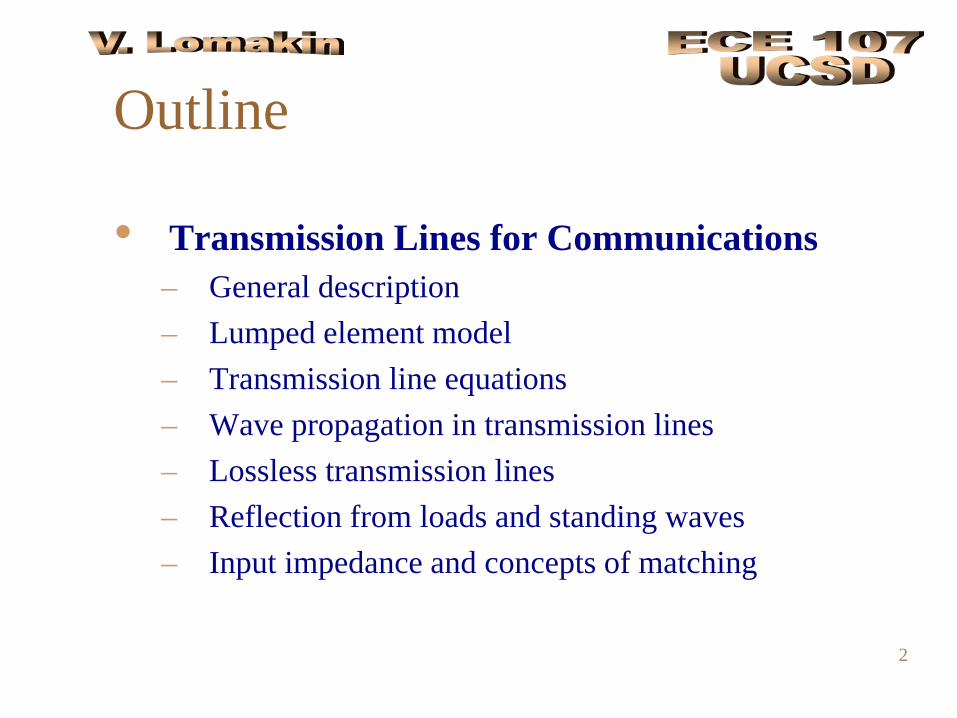
• Transmission Lines for Communications– General description– Lumped element model – Transmission line equations– Wave propagation in transmission lines– Lossless transmission lines– Reflection from loads and standing waves– Input impedance and concepts of matching
3
General description (1)
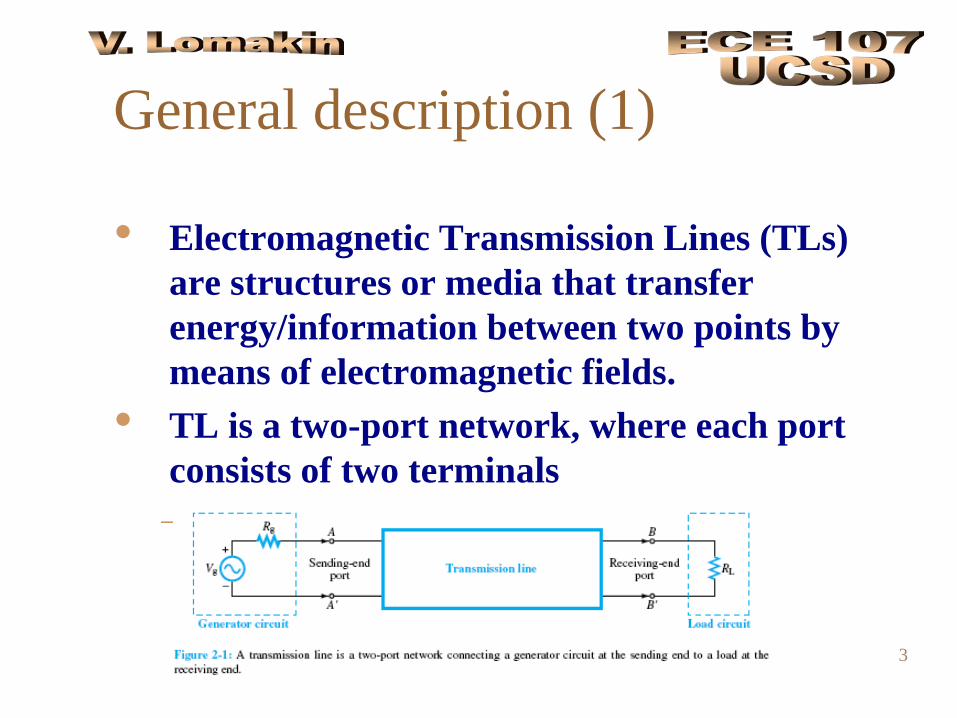
• Electromagnetic Transmission Lines (TLs) are structures or media that transfer energy/information between two points by means of electromagnetic fields.
• TL is a two-port network, where each port consists of two terminals–
4
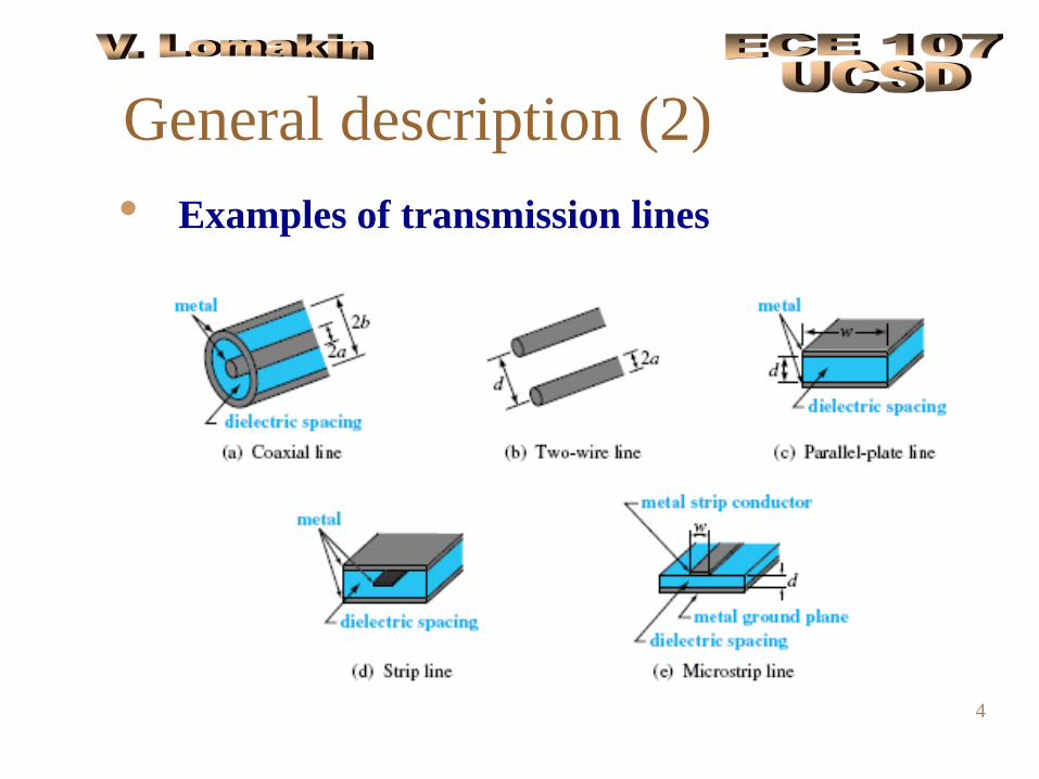
General description (2)• Examples of transmission lines
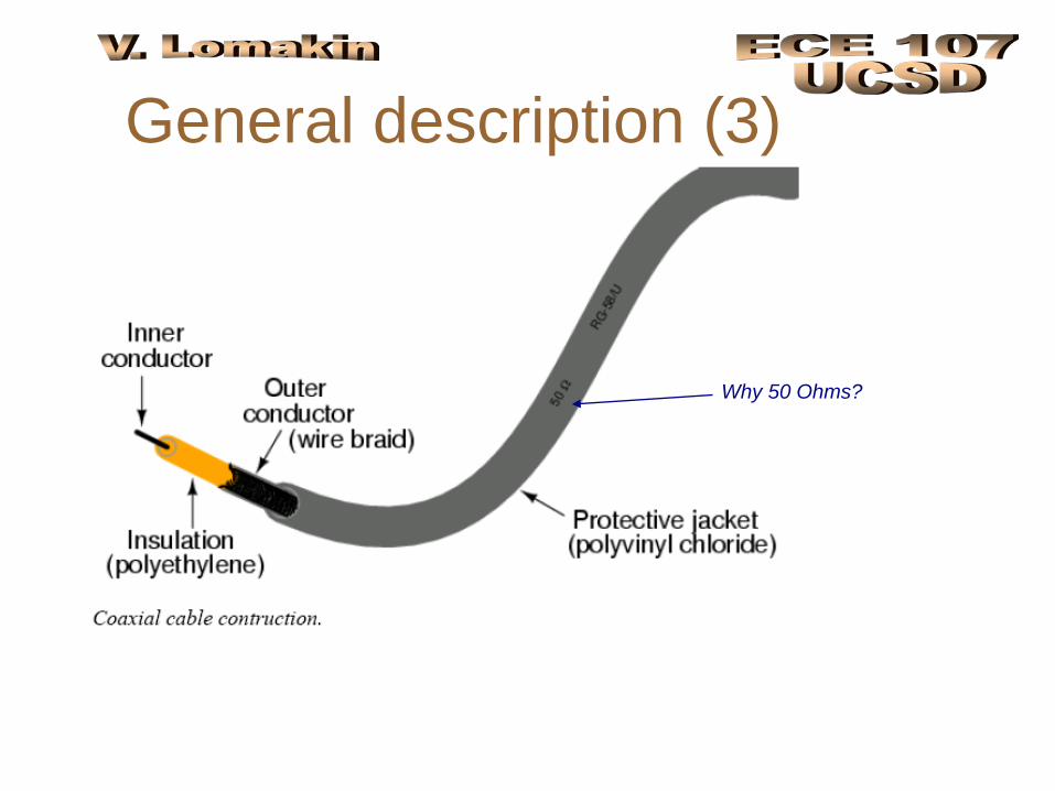
Why 50 Ohms?
General description (3)
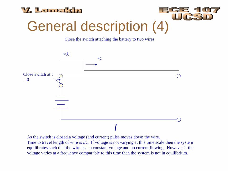
General description (4)
l
v(t)~c
As the switch is closed a voltage (and current) pulse moves down the wire.Time to travel length of wire is l/c. If voltage is not varying at this time scale then the system equilibrates such that the wire is at a constant voltage and no current flowing. However if the voltage varies at a frequency comparable to this time then the system is not in equilibrium.
Close switch at t = 0
Close the switch attaching the battery to two wires
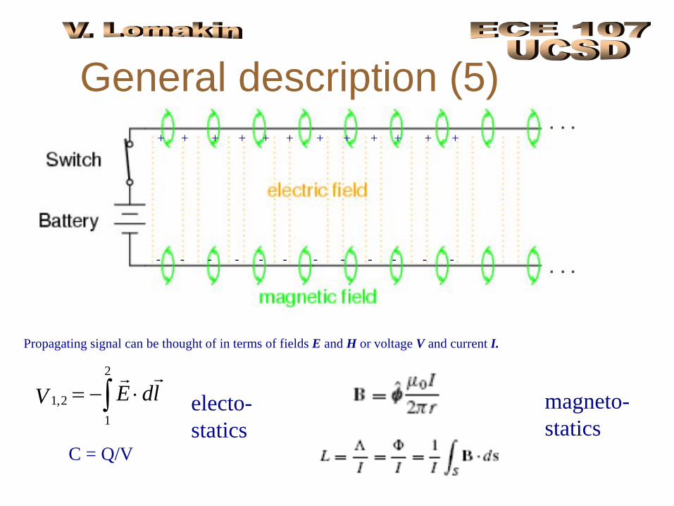
General description (5)
Propagating signal can be thought of in terms of fields E and H or voltage V and current I.
∫ ⋅−=2
12,1 ldEV
C = Q/V
+ + + + + + + + + + + +
- - - - - - - - - - - -
electo-statics
magneto-statics
8
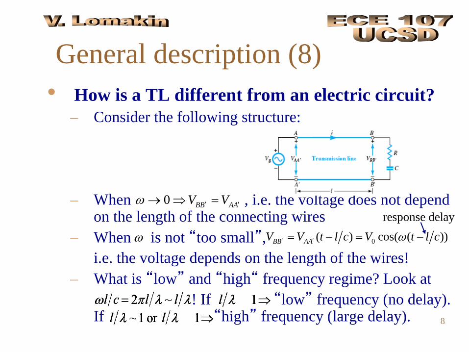
General description (8)• How is a TL different from an electric circuit?
– Consider the following structure:
– When , i.e. the voltage does not depend on the length of the connecting wires
– When is not “too small”,i.e. the voltage depends on the length of the wires!
– What is “low” and “high“ frequency regime? Look at ! If “low” frequency (no delay).
If “high” frequency (large delay).
0 BB AAV Vω ′ ′→ ⇒ =
ω 0( ) cos( ( ))BB AAV V t l c V t l cω′ ′= − = −
response delay
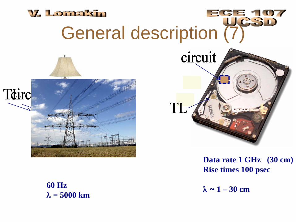
General description (7)
60 Hzλ = 5000 km
UCT)
ATE
Data rate 1 GHz (30 cm)Rise times 100 psec
λ ~ 1 – 30 cm
10
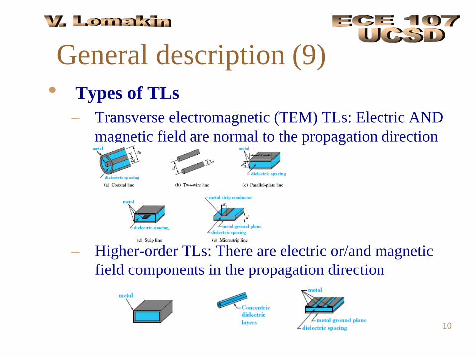
General description (9)• Types of TLs
– Transverse electromagnetic (TEM) TLs: Electric AND magnetic field are normal to the propagation direction
– Higher-order TLs: There are electric or/and magnetic field components in the propagation direction
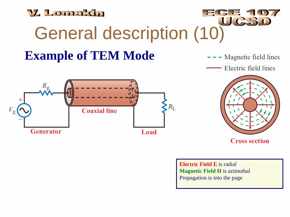
General description (10)
Electric Field E is radialMagnetic Field H is azimuthalPropagation is into the page
Example of TEM Mode
12
Lumped element model (1)• Only TEM TLs will be considered in the
course• A TL will be presented by an equivalent.
parallel-wire configuration regardless of the specific shape.
• This is allowed because the field propagates in TEM TLs independently of the cross-sectional field distribution.
• The parameters of this configuration will be different for different types of TLs.
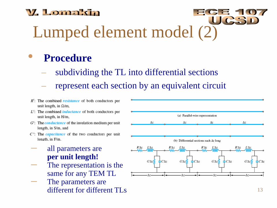
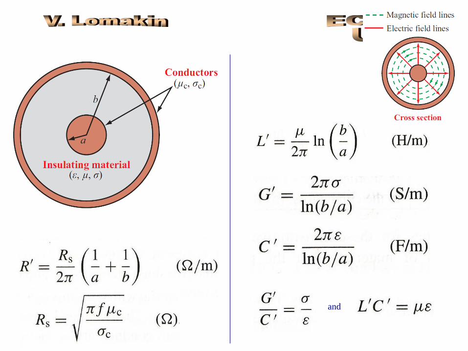
13
Lumped element model (2)• Procedure
– subdividing the TL into differential sections– represent each section by an equivalent circuit
– all parameters are per unit length!
– The representation is the same for any TEM TL
– The parameters are different for different TLs
and
15
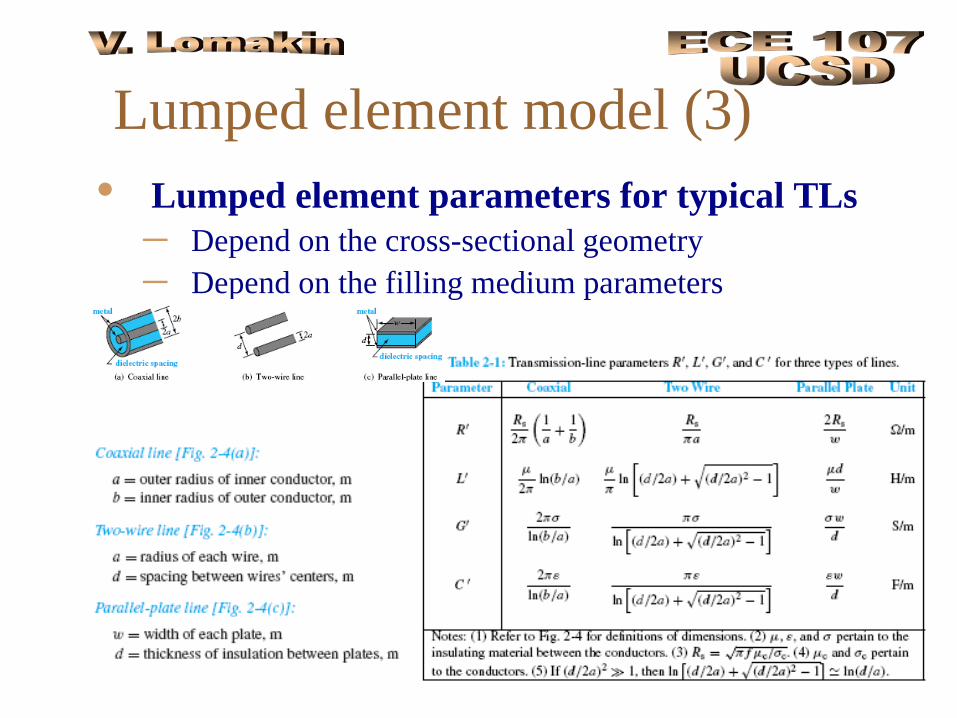
Lumped element model (3)• Lumped element parameters for typical TLs
– Depend on the cross-sectional geometry– Depend on the filling medium parameters
16
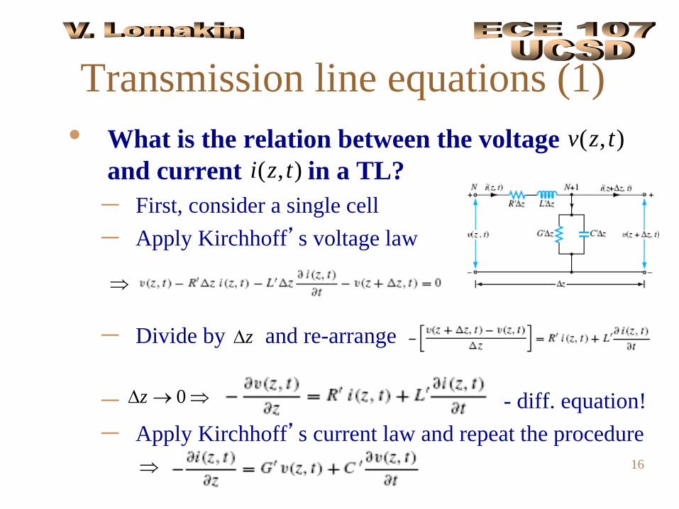
Transmission line equations (1)• What is the relation between the voltage
and current in a TL? – First, consider a single cell– Apply Kirchhoff’s voltage law
– Divide by and re-arrange
– - diff. equation!– Apply Kirchhoff’s current law and repeat the procedure
( , )v z t( , )i z t
⇒
0z∆ → ⇒
z∆
⇒
17
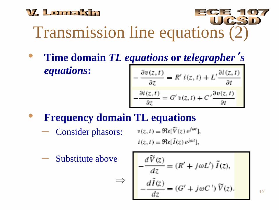
Transmission line equations (2)• Time domain TL equations or telegrapher’s
equations:
• Frequency domain TL equations– Consider phasors:
– Substitute above
⇒
18
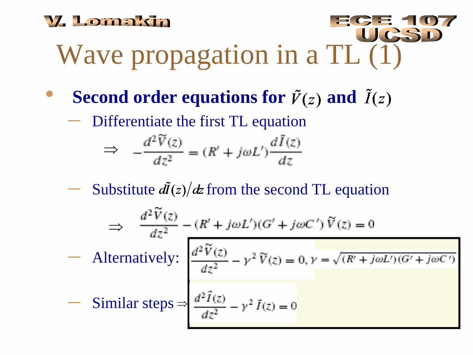
Wave propagation in a TL (1)• Second order equations for and
– Differentiate the first TL equation
– Substitute from the second TL equation
– Alternatively:
– Similar steps
⇒
⇒
⇒
19
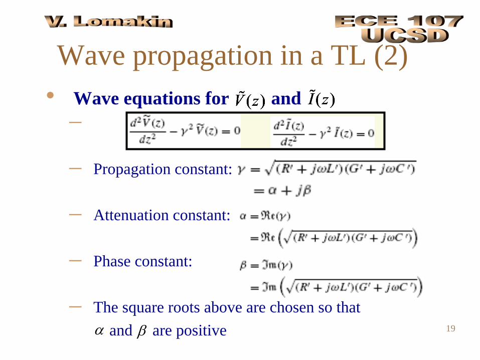
Wave propagation in a TL (2)• Wave equations for and
–
– Propagation constant:
– Attenuation constant:
– Phase constant:
– The square roots above are chosen so that and are positiveα β
20
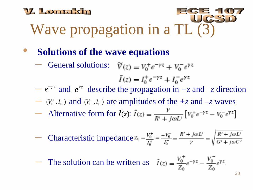
Wave propagation in a TL (3)• Solutions of the wave equations
– General solutions:
– and describe the propagation in +z and –z direction – and are amplitudes of the +z and –z waves– Alternative form for :
– Characteristic impedance
– The solution can be written as
0 0( , )V I+ +
ze γ− zeγ
0 0( , )V I− −
21
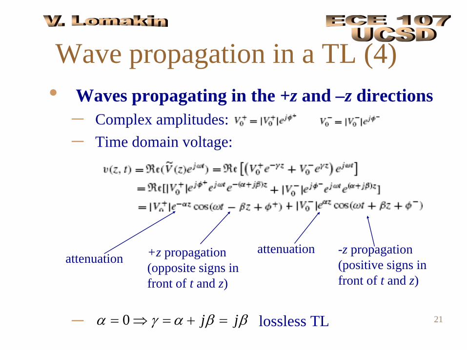
Wave propagation in a TL (4)• Waves propagating in the +z and –z directions
– Complex amplitudes:– Time domain voltage:
– lossless TL
+z propagation (opposite signs in front of t and z)
-z propagation (positive signs in front of t and z)
attenuationattenuation
0 j jα γ α β β= ⇒ = + =
22
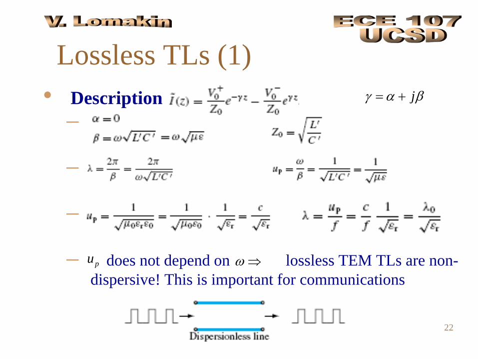
Lossless TLs (1)• Description
–
–
–
– does not depend on lossless TEM TLs are non-dispersive! This is important for communications
pu ω ⇒
jγ α β= +
23
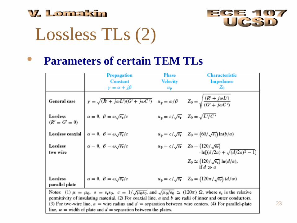
Lossless TLs (2)• Parameters of certain TEM TLs
24
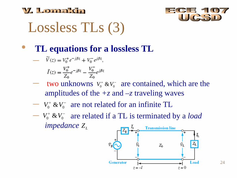
Lossless TLs (3)• TL equations for a lossless TL
–
– two unknowns are contained, which are the amplitudes of the +z and –z traveling waves
– are not related for an infinite TL– are related if a TL is terminated by a load
impedance
0 0&V V+ −
0 0&V V+ −
0 0&V V+ −
LZ
25
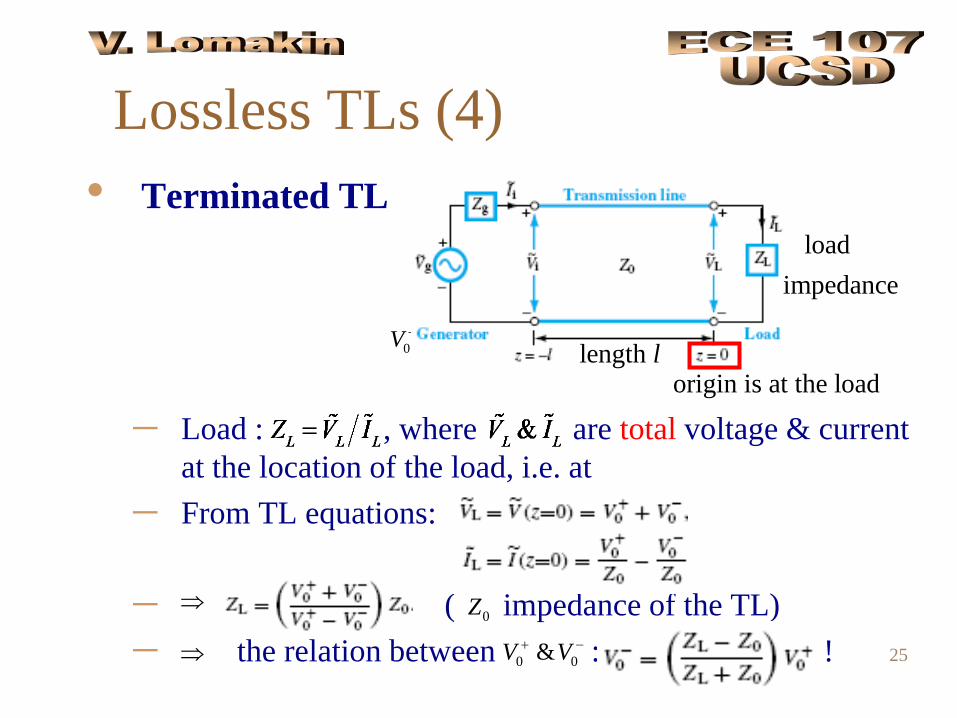
Lossless TLs (4)• Terminated TL
– Load : , where are total voltage & current at the location of the load, i.e. at
– From TL equations:
– ( impedance of the TL) – the relation between : !
0 0&V V+ −
load impedance
length lorigin is at the load
⇒0Z
⇒ 0 0&V V+ −
26
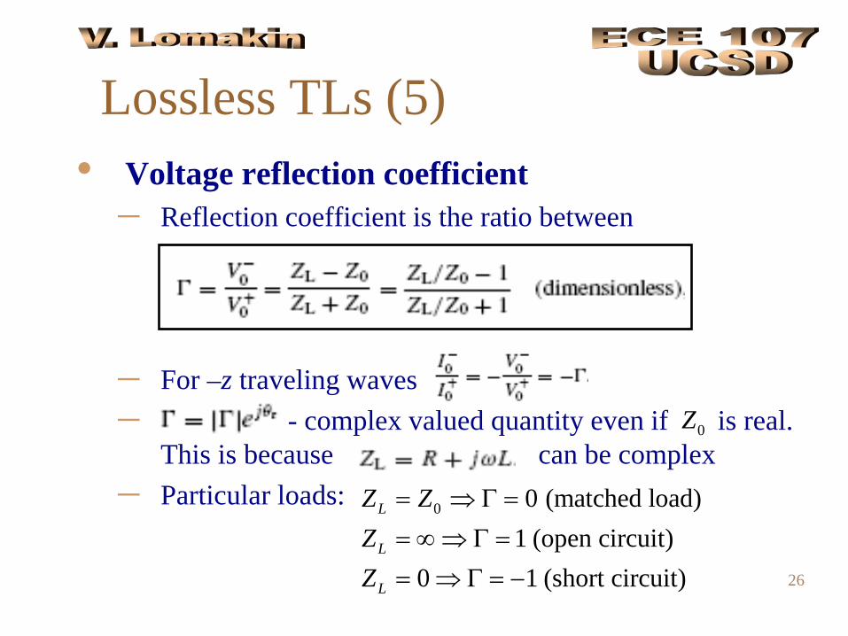
Lossless TLs (5)• Voltage reflection coefficient
– Reflection coefficient is the ratio between
– For –z traveling waves – - complex valued quantity even if is real.
This is because can be complex– Particular loads:
0Z
0 0 (matched load)1 (open circuit)
0 1 (short circuit)
L
L
L
Z ZZZ
= ⇒ Γ == ∞⇒ Γ == ⇒ Γ = −
27
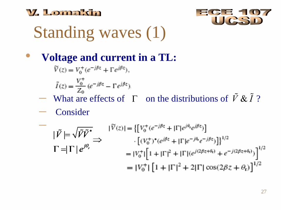
Standing waves (1)• Voltage and current in a TL:
– What are effects of on the distributions of ?– Consider–
Γ
28
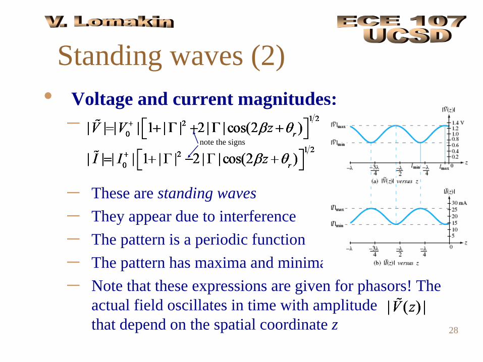
Standing waves (2)• Voltage and current magnitudes:
–
– These are standing waves– They appear due to interference– The pattern is a periodic function– The pattern has maxima and minima– Note that these expressions are given for phasors! The
actual field oscillates in time with amplitude that depend on the spatial coordinate z
note the signs
29
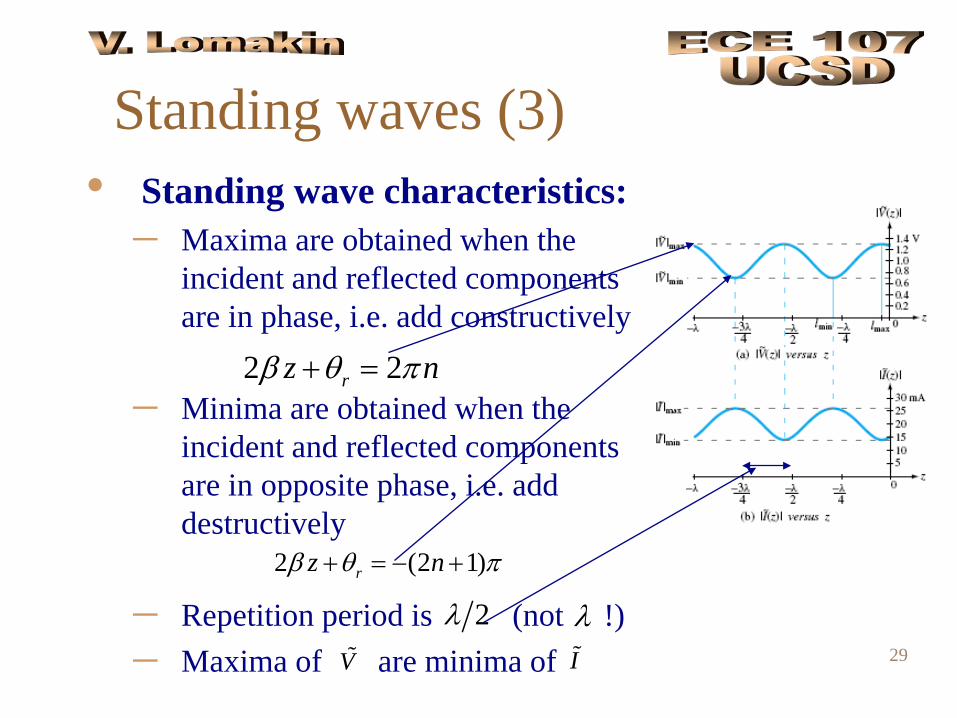
Standing waves (3)• Standing wave characteristics:
– Maxima are obtained when the incident and reflected components are in phase, i.e. add constructively
– Minima are obtained when the incident and reflected components are in opposite phase, i.e. add destructively
– Repetition period is (not !) – Maxima of are minima of
2 2rz nβ θ π+ =
2 (2 1)rz nβ θ π+ = − +
λ2λV I
30
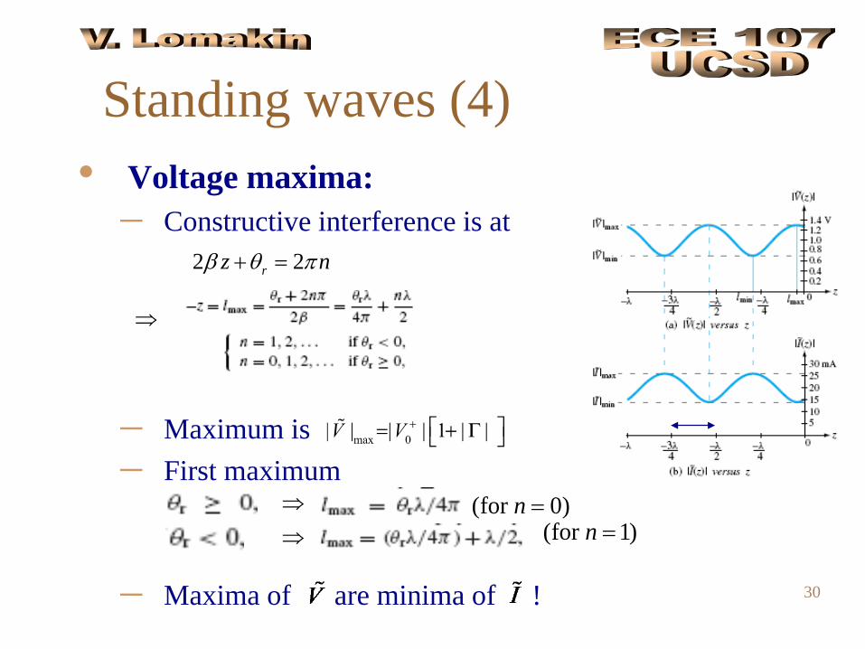
Standing waves (4)• Voltage maxima:
– Constructive interference is at
– Maximum is– First maximum
– Maxima of are minima of !
2 2rz nβ θ π+ =
⇒
⇒ (for 0)n =⇒ (for 1)n =
31
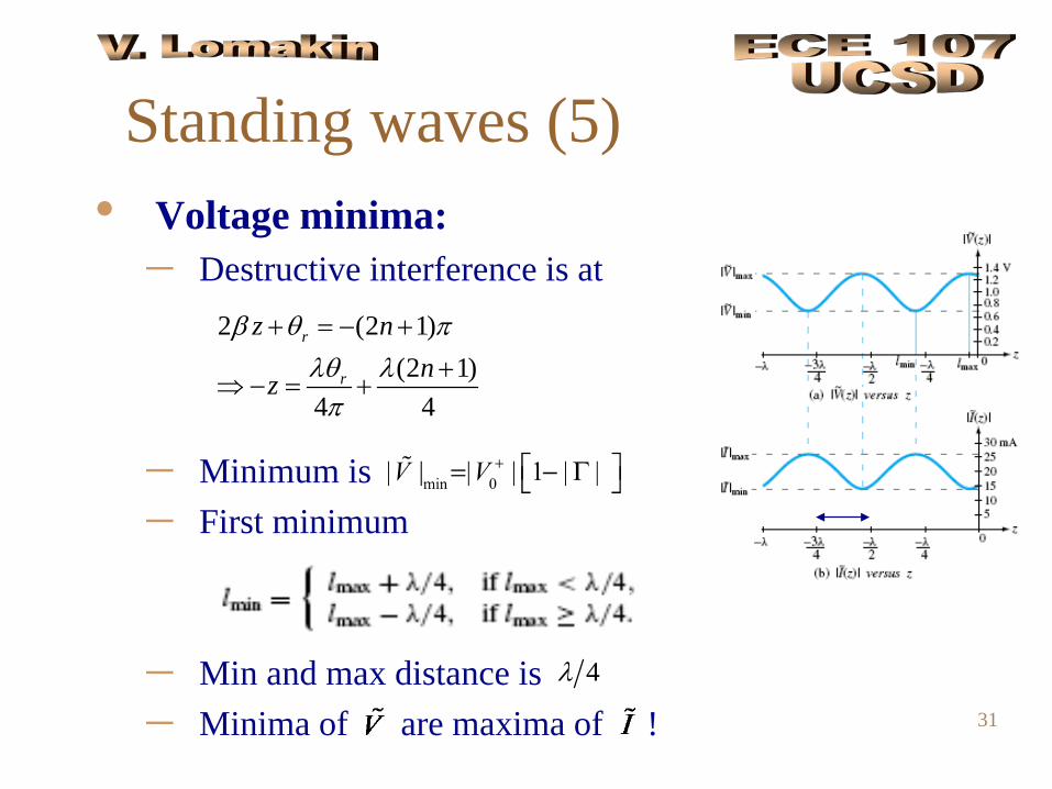
Standing waves (5)• Voltage minima:
– Destructive interference is at
– Minimum is– First minimum
– Min and max distance is– Minima of are maxima of !
2 (2 1)(2 1)
4 4
r
r
z nnz
β θ πλθ λπ
+ = − ++
⇒ − = +
4λ
32
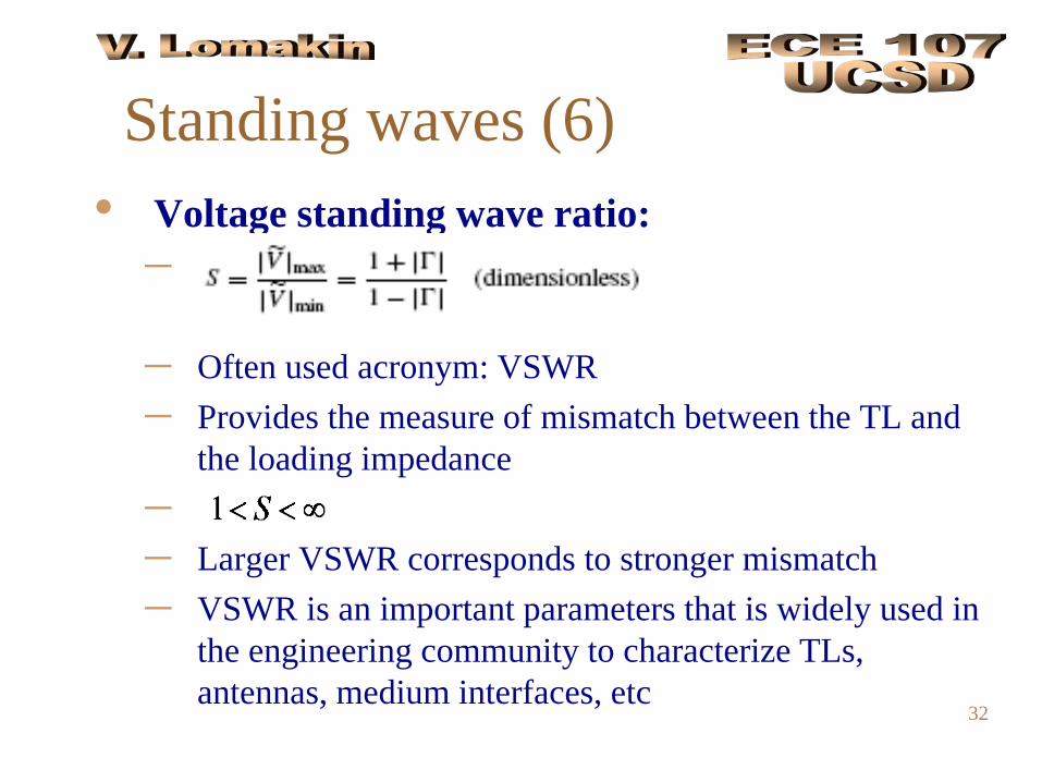
Standing waves (6)• Voltage standing wave ratio:
–
– Often used acronym: VSWR– Provides the measure of mismatch between the TL and
the loading impedance–– Larger VSWR corresponds to stronger mismatch– VSWR is an important parameters that is widely used in
the engineering community to characterize TLs, antennas, medium interfaces, etc
33
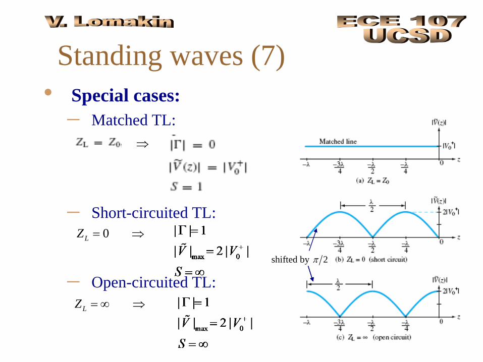
Standing waves (7)• Special cases:
– Matched TL:
– Short-circuited TL:
– Open-circuited TL:
⇒
0LZ = ⇒
LZ = ∞ ⇒
shifted by 2π
34
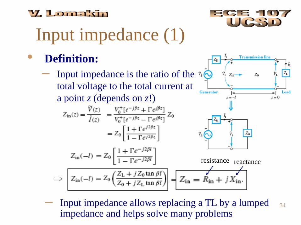
Input impedance (1)• Definition:
– Input impedance is the ratio of the total voltage to the total current at a point z (depends on z!)
⇒
– Input impedance allows replacing a TL by a lumped impedance and helps solve many problems
resistance reactance
35
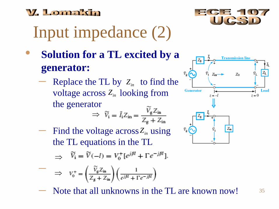
Input impedance (2)• Solution for a TL excited by a
generator:– Replace the TL by to find the
voltage across looking from the generator
– Find the voltage across using the TL equations in the TL
–
inZ
⇒
⇒
⇒
– Note that all unknowns in the TL are known now!
inZ
inZ
36
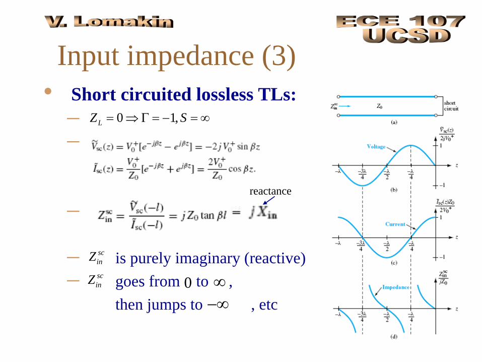
Input impedance (3)• Short circuited lossless TLs:
––
–
– is purely imaginary (reactive)– goes from to ,
then jumps to , etc
0 1,LZ S= ⇒ Γ = − = ∞
reactance
scinZscinZ ∞0
−∞
37
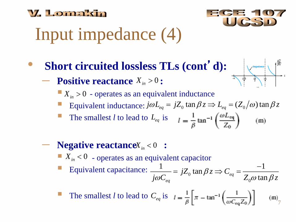
Input impedance (4)• Short circuited lossless TLs (cont’d):
– Positive reactance : - operates as an equivalent inductance Equivalent inductance: The smallest l to lead to is
– Negative reactance : - operates as an equivalent capacitor Equivalent capacitance:
The smallest l to lead to is
0inX >
0inX >
0 0tan ( ) taneq eqj L jZ z L Z zω β ω β= ⇒ =
eqL
0inX <
00
1 1tantaneq
eq
jZ z Cj C Z z
βω ω β
−= ⇒ =
0inX <
eqC
38
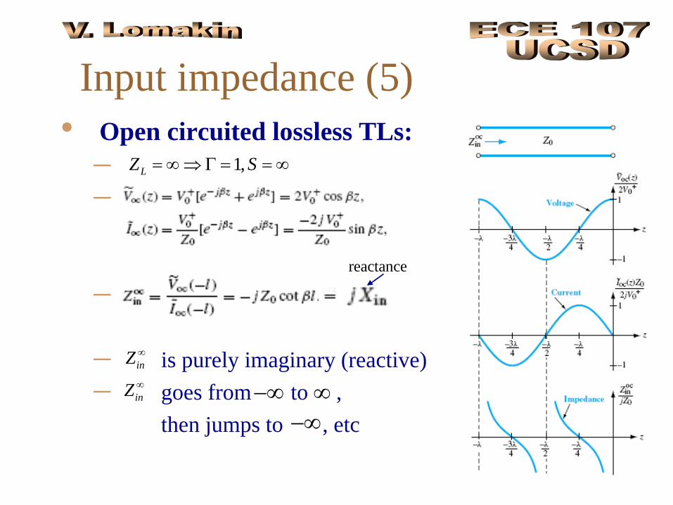
Input impedance (5)• Open circuited lossless TLs:
––
–
– is purely imaginary (reactive)– goes from to ,
then jumps to , etc
1,LZ S= ∞⇒ Γ = = ∞
reactance
inZ ∞
inZ ∞ ∞−∞−∞
39
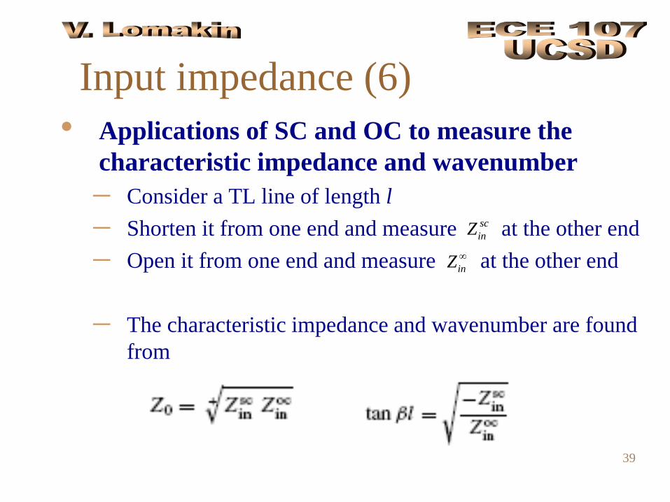
Input impedance (6)• Applications of SC and OC to measure the
characteristic impedance and wavenumber – Consider a TL line of length l– Shorten it from one end and measure at the other end– Open it from one end and measure at the other end
– The characteristic impedance and wavenumber are found from
inZ ∞
scinZ
40
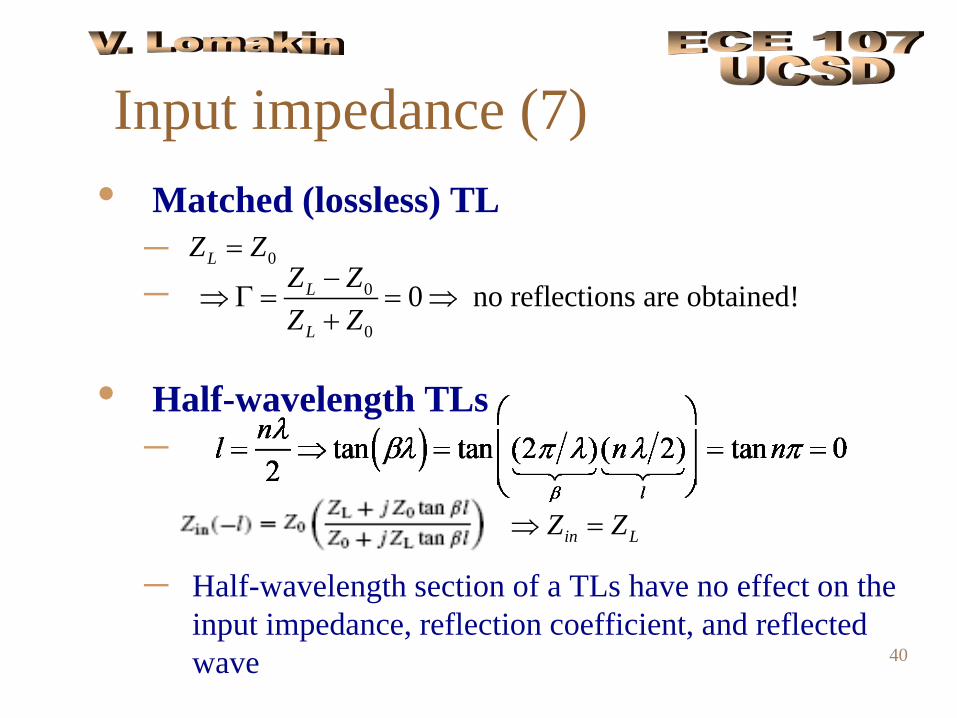
Input impedance (7)• Matched (lossless) TL
––
• Half-wavelength TLs –
– Half-wavelength section of a TLs have no effect on the input impedance, reflection coefficient, and reflected wave
0LZ Z=0
0
0 no reflections are obtained!L
L
Z ZZ Z
−⇒ Γ = = ⇒
+
in LZ Z⇒ =
41
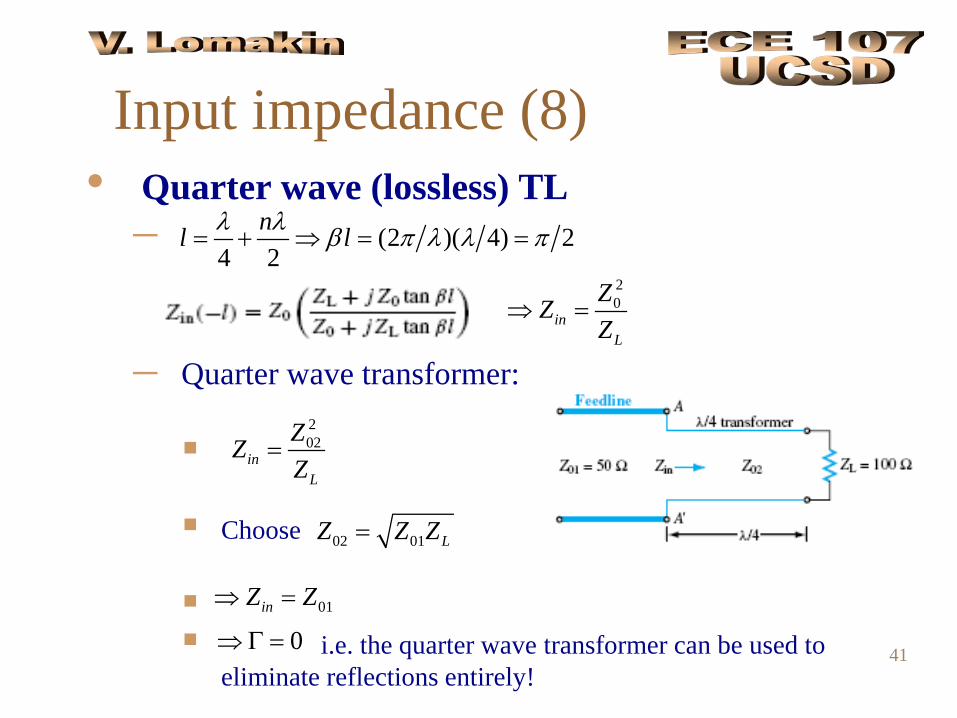
Input impedance (8)• Quarter wave (lossless) TL
–
– Quarter wave transformer:
Choose
i.e. the quarter wave transformer can be used to
eliminate reflections entirely!
(2 )( 4) 24 2
nl lλ λ β π λ λ π= + ⇒ = =
02 01 LZ Z Z=
202
inL
ZZZ
=
01inZ Z⇒ =
0⇒Γ =
20
inL
ZZZ
⇒ =
42
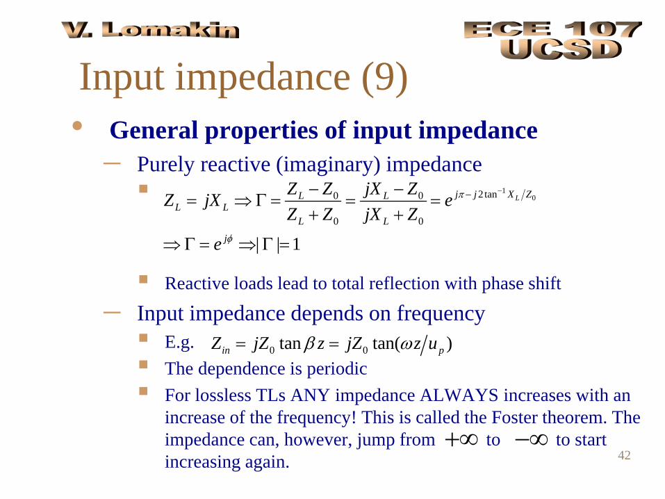
Input impedance (9)• General properties of input impedance
– Purely reactive (imaginary) impedance
Reactive loads lead to total reflection with phase shift
– Input impedance depends on frequency E.g. The dependence is periodic For lossless TLs ANY impedance ALWAYS increases with an
increase of the frequency! This is called the Foster theorem. The impedance can, however, jump from to to start increasing again.
102 tan0 0
0 0
| | 1
Lj j X ZL LL L
L Lj
Z Z jX ZZ jX eZ Z jX Z
e
π
φ
−−− −= ⇒ Γ = = =
+ +
⇒ Γ = ⇒ Γ =
0 0tan tan( )in pZ jZ z jZ z uβ ω= =
+∞ −∞
43
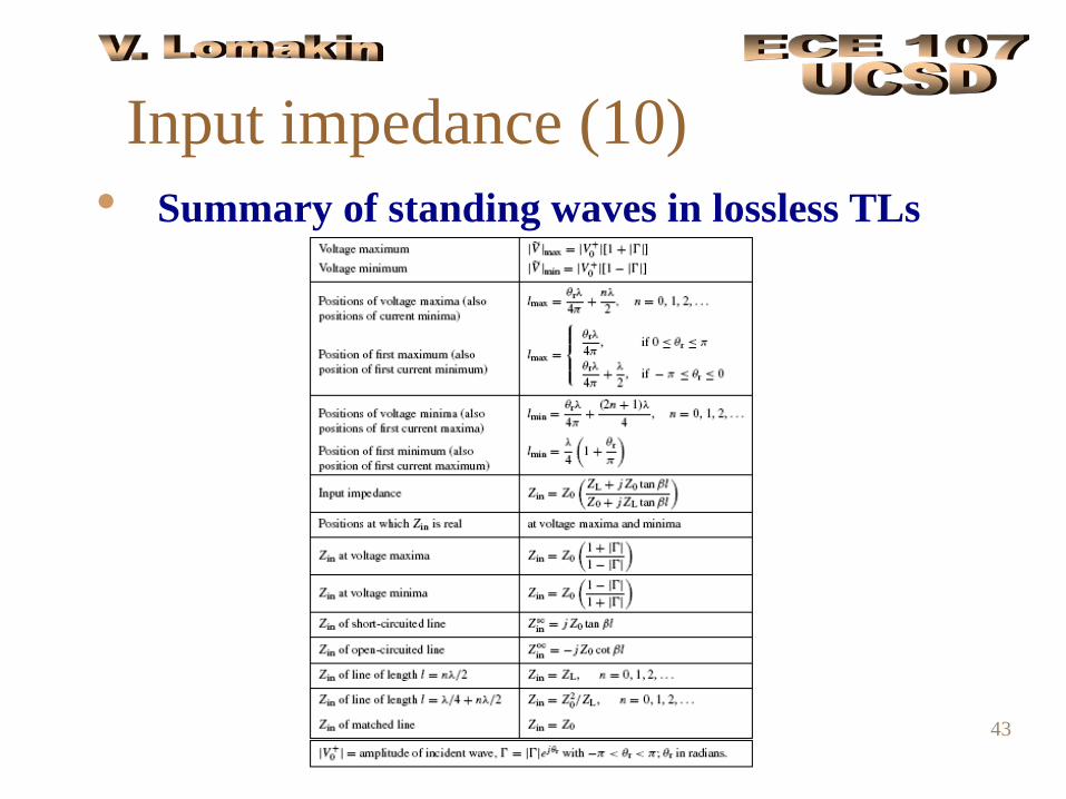
Input impedance (10)• Summary of standing waves in lossless TLs
44
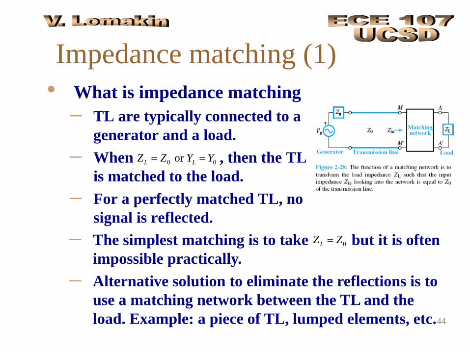
– The simplest matching is to take but it is often impossible practically.
– Alternative solution to eliminate the reflections is to use a matching network between the TL and the load. Example: a piece of TL, lumped elements, etc.
Impedance matching (1)• What is impedance matching
– TL are typically connected to a generator and a load.
– When , then the TL is matched to the load.
– For a perfectly matched TL, no signal is reflected.
0 0 or L LZ Z Y Y= =
0LZ Z=
45
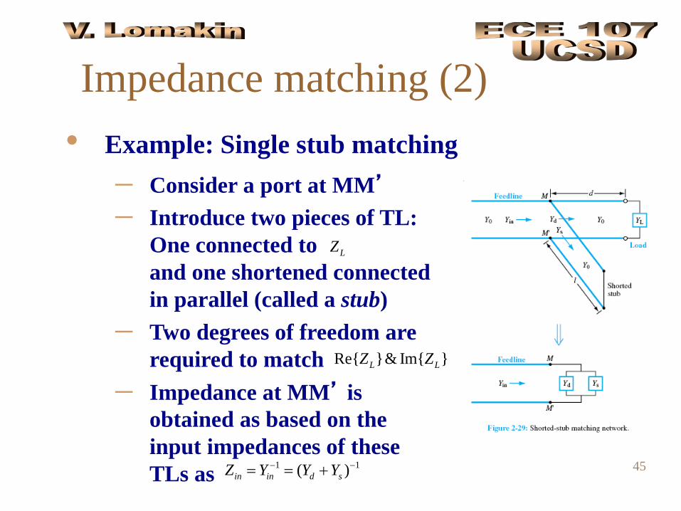
– Consider a port at MM’
– Introduce two pieces of TL: One connected to and one shortened connected in parallel (called a stub)
– Two degrees of freedom are required to match
– Impedance at MM’ is obtained as based on the input impedances of these TLs as
Impedance matching (2)• Example: Single stub matching
1 1( )in in d sZ Y Y Y− −= = +
Re{ }& Im{ }L LZ Z
LZ
46
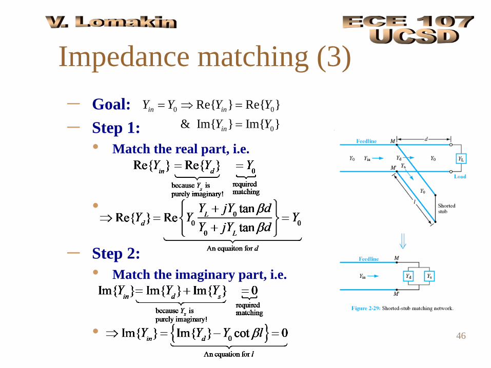
– Goal: – Step 1:
• Match the real part, i.e.
•
– Step 2: • Match the imaginary part, i.e.
•
Impedance matching (3)0 0
0
Re{ } Re{ }& Im{ } Im{ }
in in
in
Y Y Y YY Y
= ⇒ ==
47
Impedance matching (4)• General comments
– Many more options for matching networks exist– Lumped element matching is a good option as well– In most situations, perfect matching ( ) occurs
only for the matched frequency. – When the frequency is modified, the matching is not
perfect anymore, i.e. . The rate of mismatch depends on the shift of frequency and type of the matching network
0Γ =
0Γ ≠
48
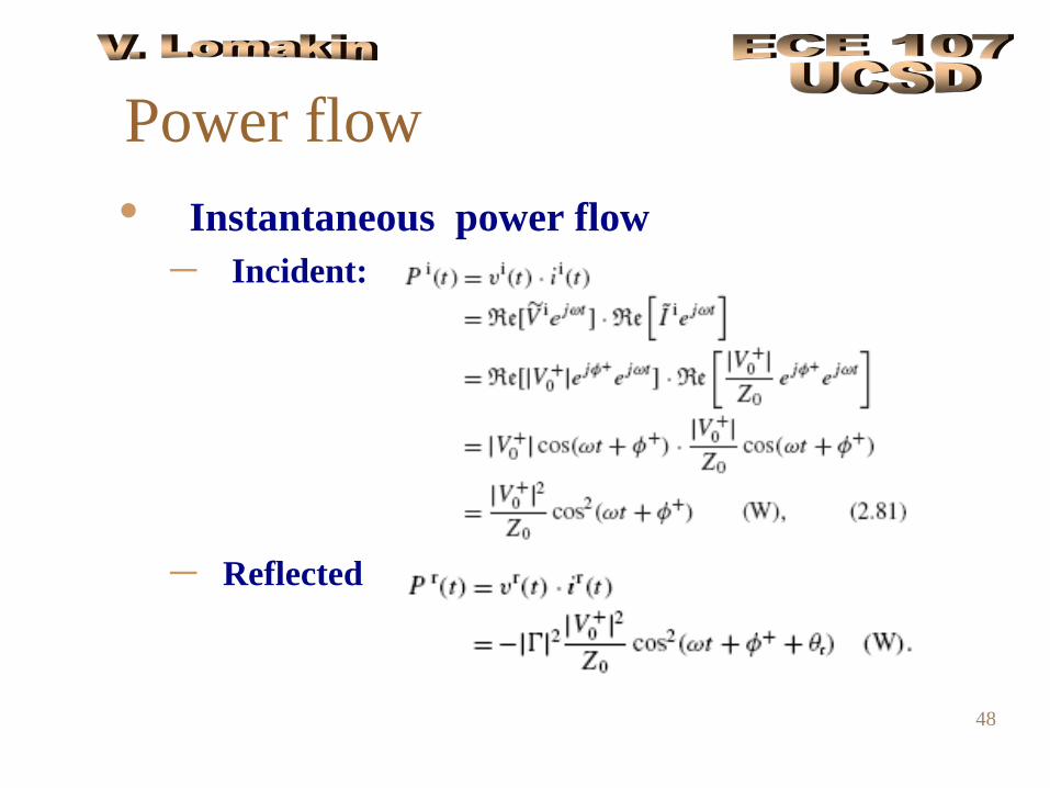
Power flow• Instantaneous power flow
– Incident:
– Reflected
49
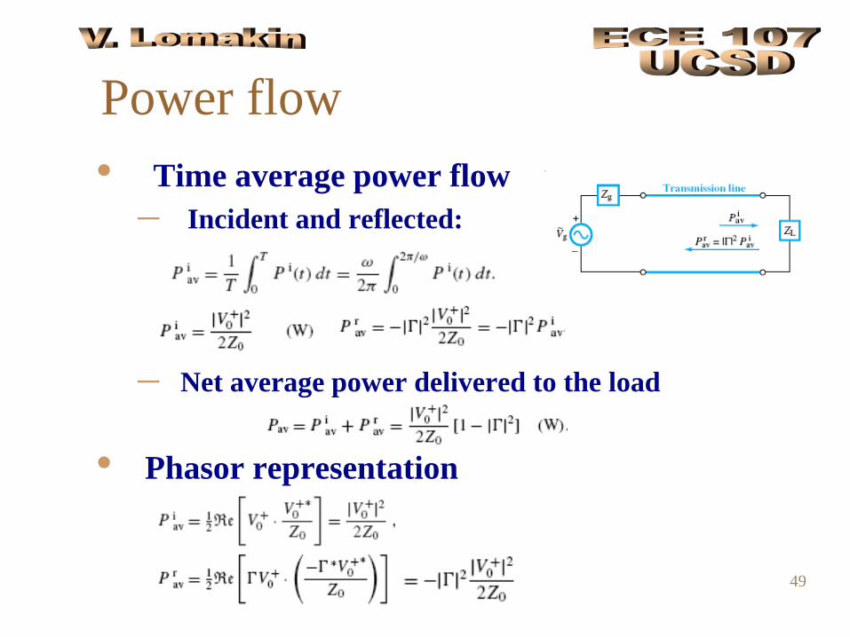
Power flow• Time average power flow
– Incident and reflected:
– Net average power delivered to the load
• Phasor representation