Embed Size (px)
Citation preview

Easy Instances for Model Checking
Markus Frick
Dissertationzur Erlangung des Doktorgrades
der Mathematischen Fakultatder Albert Ludwigs Universitat
Freiburg im Breisgau
16. August 2001

2
Dekan der mathematischen Fakultat:Prof. Dr. Wolfgang Soergel
Erster Referent:Prof. Dr. Martin Grohe
Zweiter Referent:Prof. Dr. Heinz-Dieter Ebbinghaus
Datum der Promotion: 20. Juni 2001

3
Zusammenfassung
Das zentrale Thema der vorliegenden Dissertation ist das sogenannteModel-Checking Problem. In seiner einfachsten Form haben wir eine endlicherelationale Struktur A und einen logischen Satz ϕ gegeben und fragen ob ϕin A wahr ist. Fragen dieser Art treten in den verschiedensten Bereichen derInformatik auf, unter anderem in der Datenbanktheorie und der kunstlichenIntelligenz.
Neben diesem Entscheidungsproblem untersuchen wir bestimmte Varia-tionen des Model-Checking Problems. Fur eine Formel mit freien Variablenstellen sich die Fragen des Aufzahlens aller erfullenden Belegungen, des Fin-dens einer erfullenden Belegung, sowie die Anzahl aller erfullenden Belegun-gen zu berechnen.
Unser Hauptinteresse gilt der Komplexitat dieser Probleme, wobei wir aufAlgorithmen abzielen, deren Laufzeit beliebig von der Formel, jedoch nur li-near von der Große der Eingabestruktur abhangen. Offensichtlich hangt dieKomplexitat der Model-Checking Probleme von der Ausdruckskraft der Spra-che sowie der zugelassenen Strukturen ab. So ist z.B. Model-Checking fur diemonadische Logik der zweiten Stufe (MSO) PSPACE-vollstandig. Anderer-seits hat Courcelle einen Algorithmus gefunden, der die Modellbeziehung inZeit O(f(‖ϕ‖) · ‖A‖) fur Strukturen mit Baumbreite ≤ eine fest vorgegebeneZahl w berechnet.
Die Baumbreite ist ein Maß fur die Ahnlichkeit mit einem Baum. In derAlgorithmentheorie ist diese numerische Invariante die vielleicht erfolgreich-ste Eigenschaft bei der Suche nach einfachen Instanzen fur normalerweiseharte Probleme.
In der vorliegenden Arbeit untersuchen wir im wesentlichen zwei Pro-blemarten. In Kapitel 2 verallgemeinern wir Courcelle’s Theorem und be-schreiben Algorithmen, die fur Formeln der monadischen zweiten Stufe undStrukturen beschrankter Baumbreite alle erfullenden Belegungen, bzw. eineeinzelne erfullende Belegung finden. Beide Algorithmen arbeiten in Zeit li-near in der Große der Eingabe plus der Große der Ausgabe (das ist fur denAufzahlungfall wichtig). Da das Zahlproblem bereits von Arnborg, Lagergrenund Seese im Jahre 1991 gelost wurde, kann damit MSO-Model-Checking aufStrukturen beschankter Baumbreite als vollstanding bearbeitet betrachtetwerden.

4
Die vorgestellten Algorithmen basieren auf einem automatentheoretischenAnsatz und stellen im wesentlichen nur eine Verfeinerung (und Optimierung)bereits bekannter Methoden dar.
Im zweiten Teil der Arbeit (Kapitel 3 und 4), untersuchen wir das Pro-blem der ersten Stufe Logik auf Strukturen, die lokal beschranke Baumbreitebesitzen, oder etwas formaler: fur eine Funktion f : N→ N lassen wir Struk-turen A zu, deren r-Nachbarschaften hochstens die Baumbreite f(r) haben.
Unter diesen Begriff fallen so wichtige Klassen wie planare Graphen,Strukturen beschrankter Valenz und Graphen mit beschrankter Kreuzungs-zahl.
Der Ansatz zur Losung von Model-Checking Problemen dieser Art ba-siert dabei auf der Beobachtung daß alle erste Stufe Eigenschaften “lo-kal” sind. Durch die Ergebnisse aus dem 2. Kapitel konnen nun lokaleLosungsmengen in optimaler Zeit berechnet werden (denn Nachbarschaftenhaben nach Voraussetzung beschrankte Baumbreite). Danach mussen zurLosung des jeweiligen Model-Checking Problems “nur” noch die Teilergeb-nisse zusammengesetzt werden. Auf diese Weise losen wir die vier angespro-chenen Model-Checking Probleme fur die Logik der ersten Stufe auf lokalbaumartigen Strukturen (nicely locally tree-decomposable classes). DieseAlgorithmen arbeiten alle in Zeit linear in der Große der Eingabestruktur(plus der Große der Ausgabe beim Aufzahlungsproblem). Damit ist auchdieser Problembereich vollstandig gelost.

Contents
1 Introduction 7
1.1 Background: The model-checking problem . . . . . . . . . . . 7
1.2 Preliminaries . . . . . . . . . . . . . . . . . . . . . . . . . . . 10
1.3 The road map . . . . . . . . . . . . . . . . . . . . . . . . . . . 13
2 Evaluation on Tree-like Structures 16
2.1 Tree-decompositions and linear time . . . . . . . . . . . . . . . 17
2.2 Courcelle’s result and a simple extension . . . . . . . . . . . . 21
2.2.1 Evaluation with one free point variable . . . . . . . . . 25
2.3 Evaluation on tree-like structures . . . . . . . . . . . . . . . . 28
2.3.1 Evaluating MSO-queries on colored trees . . . . . . . . 29
2.3.2 The extension to tree-like structures . . . . . . . . . . 42
3 First-Order Decision Problems 48
3.1 Local tree-likeness . . . . . . . . . . . . . . . . . . . . . . . . . 48
3.2 Gaifman’s theorem . . . . . . . . . . . . . . . . . . . . . . . . 57
3.3 The main algorithm . . . . . . . . . . . . . . . . . . . . . . . . 58
3.4 Remarks on special cases . . . . . . . . . . . . . . . . . . . . . 62
4 First-Order with free Variables 67
4.1 A normal form for local formulas . . . . . . . . . . . . . . . . 68
4.2 Including the tree cover . . . . . . . . . . . . . . . . . . . . . . 73
4.2.1 The contiguousness-graph . . . . . . . . . . . . . . . . 77
4.3 The evaluation- and witness problem . . . . . . . . . . . . . . 79
4.3.1 The evaluation problem . . . . . . . . . . . . . . . . . 80
4.3.2 Finding a witnessing tuple . . . . . . . . . . . . . . . . 85
4.4 The counting problem . . . . . . . . . . . . . . . . . . . . . . 88
4.4.1 Reducing the starting problem . . . . . . . . . . . . . . 90
4.4.2 Counting . . . . . . . . . . . . . . . . . . . . . . . . . . 94
5
6 CONTENTS
A The Machine Model 101A.1 The Definition . . . . . . . . . . . . . . . . . . . . . . . . . . . 102A.2 RAMs on relational structures . . . . . . . . . . . . . . . . . . 104A.3 Data-structures and algorithms . . . . . . . . . . . . . . . . . 105A.4 The linear time sort . . . . . . . . . . . . . . . . . . . . . . . . 111
Index 115
Bibliography 117

Chapter 1
Introduction
1.1 Background: The model-checking prob-
lem
It is an important task in complexity theory to find feasible instances forotherwise intractable problems. Apart from delivering algorithms for practi-cal use, feasibility results may shed light on the structural properties of theproblem instances. The main subject of this thesis is the so called model-checking problem and to exhibit instances for which this generally intractableproblem is easy to solve. In its basic version the problem looks as follows:we have given a structure A and a sentence ϕ and we ask whether A satisfiesϕ. If ϕ ∈ L for some logic L, we call this the L-model-checking problem.
This problem and its variations appear in various areas of computer sci-ence, most notably in database theory [CH82] and in the realm of constraintsatisfaction [FV93]. An important feature is its meta-character with respectto algorithms and complexity theory, i.e. standard problems from algorithmtheory can be expressed as certain instances of the model-checking problem.For instance, to decide if a graph G contains a k-clique, we may alterna-tively decide whether the first-order (FO) sentence ϕk, saying that there arek pairwise adjacent vertices, holds in G. In a similar way colorability can bereduced to monadic second-order (MSO) model-checking.
Essentially there are three different generalizations of the basic model-checking problem. Assume that we are given a formula ϕ with free variablesand a structure A. The evaluation problem asks for all assignments of the freevariables such that ϕ with these assignments holds in A. The case where wejust want to find a single satisfying assignment is called the witness problem,and finally, the counting problem refers to the task of computing the number
7
8 CHAPTER 1. INTRODUCTION
of satisfying assignments.
Our interest is focused on the complexity of the model-checking problemand its generalizations. This question is intimately related to the expressibil-ity of the logical language in question. First attempts of measuring the com-plexity of model-checking have been done with respect to the size ‖ϕ‖+ ‖A‖of the input. Unfortunately, this complexity turned out to be very high(and certainly depends on the chosen language); already the very basic con-junctive queries are NP-complete [CM77]. Full first-order logic and monadicsecond-order logic have been shown to be PSPACE-complete [Var82].
To prove PSPACE-hardness for FO-model-checking, we reduce the prob-lem to QBF (quantified Boolean formula, see [BDG95]), which essentially ismodel-checking over a two element structure with an unary relation. Oneconceivable interpretation of this fact is that the query carries the bulk ofcomplexity. Since at the same time, the queries are assumed to be smallcompared to the size of the structure, Vardi [Var82] introduced the notion ofData complexity. Herein, the complexity is expressed in terms of the size ofthe structure, whereas the dependency on the query is completely neglected.In this framework, we get PTIME algorithms for FO-model-checking andits generalizations, e.g. for an FO-sentence with k variables we can decideA |= ϕ in time O(‖A‖+ |A|k) [Var95].
Although this is considered to be “efficient” (well, it’s in PTIME), it isnot satisfying. Already for a query involving 5 variables and a structure ofmoderate size 1000, the algorithm needs at least 1015 steps to decide themodel relation, what is far from feasible.
Parameterized complexity is a novel approach presented by Downey andFellows [DF99]. They not only introduced new ways to measure complexity,but developed an entire complexity theory including reductions and notionsof completeness. In this framework, one or more parts of the input are con-sidered to be the parameter of the problem instance. Under these conditionsthe problem’s complexity is measured by separate functions on the parameterand the rest of the instance, respectively.
In our context, we consider the formula ϕ as the parameter and say thatmodel-checking is fixed parameter tractable (in FPT), if there is a functionf : N → N, a constant c ≥ 1 and an algorithm that solves the problemin time f(‖ϕ‖) · ‖A‖c. It was proved that conjunctive (first-order) queryevaluation is W[1]-complete [PY97] (AW[1]-complete, respectively [DFT96]).These two classes correspond to the traditional classes NP and PSPACE and
1.1. BACKGROUND: THE MODEL-CHECKING PROBLEM 9
both results entail that, unless FPT = W[1], the corresponding problems arenot in FPT.1
We employ two strategies to bypass these hardness results. The first oneis exhibiting numerical invariants of the input instances and examining thecomplexity with respect to these new parameters. The maybe most successfulparameter is the so called tree-width of a structure. Intuitively it measuresthe tree-likeness of a structure, and it has been applied to a huge varietyof algorithmic problems (cf. [Bod97] for a survey). For instance, a tree hastree-width 1, and an n-clique has tree-width n− 1. Of particular interest formodel-checking is Courcelle’s well known theorem:
Let w ≥ 1 and ϕ be a monadic second-order sentence. Then thereis an algorithm that, given a structure of tree-width at most w,decides in linear time whether ϕ holds in A.
In our framework, the tree-width w := tw(A) of A and the sentence ϕ areconsidered as parameters (actually, w is a numerical invariant of the inputstructure). Now this theorem looks as follows:
There is a function f : N2 → N and an algorithm that, given asentence ϕ ∈ MSO and a structure A, decides whether ϕ holds inA in time
f(‖ϕ‖, tw(A)) · ‖A‖.
The second, less general approach we follow in this thesis, is to apriori re-strict the class of admitted structures. For a long time it has been known thatproperties expressible in first-order logic are local [Gai82]. Hence, motivatedby Courcelle’s theorem, it is conceivable that local tree-likeness of structurescan be exploited to get efficient algorithms. In this thesis, we introduce thenotion of locally tree-decomposable classes C and show the following:
Let C be a locally tree-decomposable class of structures. Thenthere is an f : N → N and an algorithm that, given an FO-sentence ϕ and a structure A ∈ C, decides whether ϕ holds in A
in timef(‖ϕ‖) · ‖A‖.
Many important classes are locally tree-decomposable, for example, theclass of graphs of bounded genus and graphs with bounded valence. Note
1Like NP 6= P, it is usually assumed that FPT 6= W[1].

10 CHAPTER 1. INTRODUCTION
here that Courcelle’s theorem is a uniform result, in the sense that thereis one algorithm that works for all input structures. In contrast to that,this second approach gives for each class C an algorithm solving the model-checking problem for structures from C.
All results presented in this thesis are essentially of the two types above.For the decision, witness and counting problems, we aim at algorithms thatwork within time linear in the size of the input structure. For the evaluationcases we admit time linear in the size of the input structure plus the size ofthe output. In particular, we will settle the MSO-evaluation problem andthe MSO-witness problem in linear time parameterized by the tree-width ofthe input structure. Furthermore, we are able to extend the just mentionedoptimal model-checking result for locally tree-decomposable classes to theevaluation, witness and counting cases.
Before we give a survey on the thesis and an exact formulation of theproved results, we have to fix notation and the computation model.
1.2 Preliminaries
For n ≥ 1, we set [n] := 1, . . . , n. By Pow(A) we denote the power set ofA and Pow≤l(A) is the set of elements of Pow(A) that have cardinality ≤ l.
A vocabulary is a finite set of relation symbols. Each relation symbol isassociated with a natural number, its arity. Vocabularies are always denotedby the letter τ .
A τ -structure A consists of a non-empty set A, called the universe of A,and a relation RA ⊆ Ar for each r-ary R ∈ τ . Let A be a structure andB ⊆ A non-empty. Then 〈B〉A denotes the substructure of A induced by B.If the context is clear we omit the superscript.
We only consider finite structures. A graph is an E-structure (G,EG)where EG is an anti-reflexive and symmetric binary relation (in otherwords: we consider simple undirected graphs without loops). The ele-ments of the universe of a graph are called vertices and sometimes we re-fer to elements of EG by the term edges. A colored graph is a structureB = (B,EB, PB
1 , . . . , PBm ), where (B,EB) is a graph and the unary relations
PB1 , . . . , P
Bm form a partition of the universe B.
For a vocabulary τ , the set of first-order formulas is built up from aninfinite supply of variables x, y, x1, x2, . . ., the relation symbols R ∈ τ and =,

1.2. PRELIMINARIES 11
the connectives ∨,∧,¬,→ and the quantifiers ∀x, ∃x ranging over elementsof the universe of the structure. This logic is denoted by FO.
We extend this calculus by unary second-order variables X,Y,X1, X2, . . .which range over sets of elements of the universe. For a vocabulary τ , themonadic second-order logic (MSO) is the closure of FO under the adjunctionof the new atoms built from new unary relation variables, and unary second-order quantification ∃X,∀X.
A free variable in a formula ϕ is a variable x (or X) occurring in ϕ thatis not in the scope of a quantifier ∃x, ∀x (or ∃X,∀X, respectively). We writeϕ(X1, . . . , Xl, x1, . . . , xm) to indicate that the free variables in ϕ are exactlyX1, . . . , Xl, x1, . . . , xm. A sentence is a formula that contains no free vari-ables. The semantics of FO,MSO should be clear. For a τ -structure A,A1, . . . , Al ⊆ A, a1, . . . , am ∈ A and a τ -formula ϕ(X1, . . . , Xl, x1, . . . , xm) wewrite A |= ϕ(A1, . . . , Al, a1, . . . , am) to say that A satisfies ϕ if the variablesX1, . . . , Xl are interpreted by the subsets A1, . . . , Al and x1, . . . , xm are inter-preted by the elements a1, . . . , am, respectively. The rank rk(ϕ) of a formulaϕ is the maximal number of nested quantifiers in ϕ.
For a structure A and a formula ϕ(X1, . . . , Xl, x1, . . . , xm) we let
ϕ(A) := (A1, . . . , Al, a1, . . . , am) | A |= ϕ(A1, . . . , Al, a1, . . . , am).
For a sentence ϕ we set ϕ(A) = TRUE if A satisfies ϕ, and = FALSE,otherwise2. If the vocabularies of A and ϕ do not agree, we set ϕ(A) =FALSE (or = ∅ for ϕ with free variables). Here the convention that allvariables of ϕ enclosed within the brackets actually occur freely in ϕ is crucialfor this definition to be well defined.
Let L be a logic and C a class of structures (C may be the class of allstructures). The L-model-checking problems over C are the following:
• the decision problem
Input: Structure A ∈ C, sentence ϕ ∈ L.Problem: Decide, if ϕ(A) = TRUE.
• the evaluation problem
2To be more consistent, we could define TRUE = ∅ and FALSE = .

12 CHAPTER 1. INTRODUCTION
Input: Structure A ∈ C, formula ϕ ∈ L.Problem: Compute ϕ(A).
• the witness problem
Input: Structure A ∈ C, formula ϕ ∈ L.Problem: Compute an element of ϕ(A).
• the counting problem
Input: Structure A ∈ C, formula ϕ ∈ L.Problem: Compute |ϕ(A)|.
Algorithms: Since we are looking for linear time algorithms for the abovequery evaluation problems, the questions of how the input is coded and whatmodel of computation we employ, become a central issue. Our underlyingmodel of computation is the standard RAM-model with addition and sub-traction as arithmetic operations [AHU74]. We assume the logarithmic costmeasure. For an exact description of the model, and why we have chosen it,we refer the reader to the appendix (section A). There we also give a descrip-tion of the pseudo-code we use in the algorithms. Nevertheless, it should bepossible to understand the programs without reading the appendix.
In our main results, we mostly omit the O-notation. This improves read-ability of the main results (and often we can think of the constants as part ofsome unspecified function bounding the running time: e.g. f in f(‖ϕ‖)·‖A‖).But it should be clear that all results involve constants depending on the usedhardware and data-structures.
A relational structure A is coded by a word w consisting of the vocabulary,the elements of the universe A, and the relations RA for R ∈ τ . Observe thatwe do not encode relations by the corresponding Boolean matrices, but simplyby a list of its tuples. This is considered the standard coding for algorithms.It becomes particular important due to the fact that we develop algorithmsrunning in time linear in the size of the input structure. In that case codingrelations by their Boolean matrices would waste space and grant too muchtime, if the relations contained few tuples. Again, we refer the reader to theappendix (section A.2).
Formulas are coded in some reasonable way, e.g. by a string or its syn-tactic tree.
1.3. THE ROAD MAP 13
We will carefully distinguish between the size ‖o‖ of an object o (whichis the length of the used encoding), and, if o is a set, its cardinality |o|. Forinstance, if R is an r-ary relation, then ‖RA‖ = O(r ·|RA|+1). The differencebetween | · | and ‖ · ‖ becomes crucial when we consider sets of the form ϕ(A)where ϕ has free second-order variables.
As an example let us present an easy observation concerning the decisionproblem for first-order logic over the class of all structures.
Example 1 ([Var95]). Let ϕ(x) ∈ FO with k variables. Then ϕ(A) can becomputed in time
O(‖ϕ‖(‖A‖+ |A|k))
Proof: First, check if ϕ(x) and A are of the same vocabulary and, if not,return ∅.
Let all variables in ϕ be among x1, . . . , xk. As a matter of fact, there areO(‖ϕ‖) many subformulas ψ1(x), . . . , ψm(x) of ϕ(x). We compute ψi(A) ina bottom-up manner. We start with the atoms, i.e. if ψi(x) is of the formRx for some R ∈ τ then ψi(A) can easily be computed by a loop over theelements of RA. If ψi is a conjunction or negation, then simply take the joinor complement of the corresponding intermediate result(s).
Let e.g. (x1, . . . , xl) be the tuple of variables free in ψj and ψi(x) =∃x1ψj(x). Now compute the projection of ψj(A) without the coordinatecorresponding to x1. The result is ψi(A).
Since for all i |ψi(A)| ≤ |A|k it is easy to see that the algorithm, suitablyimplemented, works within the claimed time bound. 2
1.3 The road map
So let us give a survey on the thesis. As mentioned before, our main topicis the model-checking problem and its generalizations. We start with anoverview of the most relevant results and give some hints about how theseresults have been achieved.
In the second chapter, we examine the MSO-model-checking problemsover structures of bounded tree-width. The standard way to handle thiskind of problems, is to reduce the problem stated for arbitrary structures toa problem on binary trees. This linear time reduction was first employed in[ALS91]. The resulting problem instance is well suited to apply, the algo-rithmically well understood, automata theoretic methods.
14 CHAPTER 1. INTRODUCTION
We proceed in a two-fold way. First, we re-prove Courcelle’s theorem,which coincides with the decision problem for MSO-logic parameterized bythe tree-width of the input structures. This is done without the abovemen-tioned reduction using merely logical methods. Using dynamic programmingthis approach is extended to solve the evaluation problem for formulas witha single free first-order variable.
After that, we turn to the standard approach. We develop algorithms forthe evaluation and witness problem, i.e. algorithms that, given a structure A
and an MSO-formula ϕ(X, y), compute ϕ(A) in time f(‖ϕ‖, w) · (‖ϕ(A)‖ +‖A‖), for some function f : N2 → N and w the tree-width of A (and in timef(‖ϕ‖, w) · ‖A‖ for the witness problem).
The proofs do not contain essentially new ideas. Some ideas concerningautomata can already be found in [CM93] (although no effort was made inoptimization). So the main technical problem remained to achieve the tighttime bounds.
Observe that the counting problem for MSO over structures of boundedtree-width has already been settled by Arnborg, Lagergren and Seese[ALS91].
The third chapter is dedicated to the problem of deciding first-order prop-erties over locally tree-decomposable classes of structures. Essentially, a classC of structures is locally tree-decomposable, if for each A ∈ C the universeA can be covered suitably by a family T of subsets of A, such that for eachT ∈ T , 〈T 〉A has tree-width bounded by a value independent from the sizeof A. After giving the definition, we prove some lemmas about the structureof such classes.
Several natural classes of structures happen to be locally tree-decomposable. Most notably structures of bounded degree, structures ofbounded tree-width, planar graphs, and graphs embeddable into some sur-face.
Then we prove the main theorem saying that over classes C of locallytree-decomposable classes, the FO-decision problem is solvable in linear time.More precisely, there is a function f : N → N and an algorithm that, givena structure A ∈ C and an FO-sentence ϕ, decides if ϕ holds in A in timef(‖ϕ‖) · ‖A‖. Roughly, we use the normal form theorem from Gaifman[Gai82] that allows to express first-order definable queries by “local” queries.These local queries can be evaluated in the substructures induced by thecover sets (the T ’s in the above definition). In a last step, we re-assemble thelocal results and decide whether the initial first-order sentence holds in A.

1.3. THE ROAD MAP 15
A natural continuation of the third chapter is to extend the decision re-sult to the cases with free variables. This is what the forth chapter intends.But unfortunately, to solve these problems in the affirmative, the class char-acterization developed in the preceding section does not suffice. We will callclasses satisfying a more restricted definition nicely locally tree-decomposable.A pleasant property of this new, stricter definition is that it still comprisesall examples mentioned above.
For such classes of structures we develop algorithms that solve the evalu-ation and witness problem. Given an input structure A and a formula ϕ(x),the running time is bounded by f(‖ϕ‖) · (|ϕ(A)| + ‖A‖) for the evaluationproblem and by f(‖ϕ‖) · ‖A‖ for the witness problem.
The details are too involved to be presented here, but essentially we againexploit locality and use the fact that local computations can be done inoptimal time (by the results of the second chapter for structures of boundedtree-width).
Finally, we attack the FO-counting problem for nicely locally tree-decomposable classes. At the end of the forth chapter, this counting problemis reduced to the calculation of a sum over labels attached to “independent”sets of a graph of bounded degree (hence we have a polynomial number ofaddends). Nevertheless, we get an algorithm that solves the FO-countingproblem over such classes in time f(‖ϕ‖) · ‖A‖ for some suitable functionf : N→ N and input A, ϕ.
In the appendix we will present the machine model and some basic algo-rithms that are used in the thesis.
Thanks to my supervisor Martin Grohe for guidance and advice. I wouldalso like to thank all people giving useful comments on drafts of this thesis(they know who they are). Particular thanks to Bernhard Herwig who in thelast minute pointed out an easy proof for theorem 67.
Chapter 2
Evaluation on Tree-likeStructures
Intuitively, the tree-width of a graph measures its similarity with a tree.In the known form, this notion was introduced by Robertson and Seymour[RS86], and the straightforward generalization to arbitrary structures is dueto Feder and Vardi [FV93].
We start with the introduction of the notion of a tree-decomposition forarbitrary structures. To explain the handling of such decompositions, wedevelop the adequate data structures and procedures that are essential forlinear time algorithms. As a first application, we re-prove Courcelle’s theo-rem [Cou90] by purely logical techniques. In a further step, we extend thisresult by a Dynamic programming approach to a linear time algorithm thatassociates to each element of the input structure its logical type.
In the subsequent section we state and prove the main result concerningstructures of bounded tree-width. It claims that there is an algorithm thatevaluates MSO-queries in time linear in the size of the input plus the sizeof the output. This is done by an automata theoretic approach, essentiallybased on ideas from Arnborg, Lagergren and Seese [ALS91]. For that, thequestion about tree-decompositions is reduced to colored binary trees, onwhich (by [TW68]) MSO and deterministic tree automata coincide. Doing asuitable prescan, we will be able to avoid unnecessary computation, and thusobtain the tight time bound. In a paper of Courcelle and Mosbah about eval-uating MSO on tree-like graphs [CM93] it was already noted that the usualautomata theoretic methods can be improved by sorting out unreachablestates. But neither the exact idea was made explicit nor an implementationwas given to obtain optimal time bounds. In fact, these details will be thetechnically most involved part of the section.
16

2.1. TREE-DECOMPOSITIONS AND LINEAR TIME 17
2.1 Tree-decompositions and linear time
We start with the definition of a tree-decomposition of a relational structure.Recall that a tree is a connected acyclic graph. Let A be a τ -structure forsome relational vocabulary τ .
Definition 2. A tree-decomposition of A is a pair (T , (Bt)t∈T ), where T isa tree and (Bt)t∈T is a family of subsets of A such that
(1) For every a ∈ A, the set t ∈ T | a ∈ Bt is non-empty and connectedin T .
(2) For every R ∈ τ and every a ∈ RA there is a t ∈ T such that a ∈ Bt.
The sets Bt are called the blocks of the tree-decomposition, and the widthof (T , (Bt)t∈T ) is max|Bt| | t ∈ T − 1. The tree-width tw(A) of A isthe minimal width of a tree-decomposition of A. From property (1) weimmediately derive the following important property of tree-decompositions:Let t, t′ ∈ T with common ancestor s. Then Bt ∩Bt′ ⊆ Bs.
Sometimes we use the easy fact that the class of structures of tree-widthat most w is sparse:
Lemma 3 ([Bod98]). Let w ≥ 1 and τ a vocabulary. Then there is aconstant k (depending on τ and w) such that for every τ -structure A of tree-width at most w we have ‖A‖ ≤ k · |A|.
The main application of this fact is that if C is a class of structures oftree-width ≤ w, then each relation of a structure A ∈ C contains at mostf(w, τ) · |A| many tuples for some suitable f : N2 → N. Hence, we can passthrough the relation in time linear in the cardinality of the universe.
Definition 4 (Gaifman graph). Let A be a τ -structure. Then the Gaifmangraph of A is the graph G(A) = (G,EG(A)), with universe G := A and an edgebetween a, b ∈ A, a 6= b, if there is an R ∈ τ and a tuple (a1, . . . , ak) ∈ RA
such that a, b ∈ a1, . . . , ak.It is easy to see that, given a structure A, its Gaifman graph G(A) can
be calculated in time O(‖A‖): For each k-ary relation R ∈ τ perform a loopover all (a1, . . . , ak) ∈ RA doing the following: for each i = 1, . . . , k add aito the adjacency list of a1, . . . , ai−1, ai+1, . . . , ak, respectively. Afterwards,we remove multiple vertices from every adjacency list (cf. end of sectionA.3). The time bound is easily verified. Observe here that the constanthidden behind the O-notation depends on the vocabulary τ . If r denotesthe maximal arity of relations of τ then the constant is roughly |τ | · r2 (each(a1, . . . , ak) ∈ RA leads to at most k(k − 1) edges in the Gaifman graph).
The next property of Gaifman graphs is particularly useful:

18 CHAPTER 2. EVALUATION ON TREE-LIKE STRUCTURES
Lemma 5. Let A be a τ -structure. Then (T , (Bt)t∈T ) is a tree-decompositionof A if, and only if, it is a tree-decomposition of G(A).
Proof: Assume that (T , (Bt)t∈T ) is a tree-decomposition of G(A). Now takean a ∈ RA, for some R ∈ τ . Since in G(A) the set a1, . . . , ak is a clique,it must appear in a single block Bt, hence a ∈ Bt. The connectedness (1)condition is equal for both, the structure and its Gaifman graph.
For the other direction, assume that (T , (Bt)t∈T ) is a tree-decompositionof A and (a, b) ∈ EG(A). By definition of the Gaifman graph, there is anR ∈ τ and an a ∈ RA such that (a, b) ∈ a1, . . . , ak. Thus, there is a t ∈ Tsuch that a ∈ Bt, hence (a, b) ∈ Bt. 2
By this lemma, most results about tree-decompositions of graphs extendto structures. In particular, the outstanding result that tree-decompositionscan be calculated in linear time was originally stated for graphs.
Theorem 6 (Bodlaender[Bod96]). There is a polynomial p(x) and analgorithm that, given a τ -structure A, computes a tree-decomposition of A ofwidth w := tw(A) in time
O(2p(w)|A|).
The first problem with this algorithm is that it is technically so involvedthat an implementation appears to be hopeless. On the other hand the factordepending on w grows unreasonably high, even small values. This makes thealgorithm almost worthless for practice. A Dynamic programming approachto the problem has been developed by Arnborg et al [ACP87]. This, atleast implementable, algorithm needs O(|A|w+1) time to compute a tree-decomposition of width w := tw(A). But due to its Dynamic nature, this isalso the least running time, hence it can not even be used for a particular setof instances. Until now there is no practical algorithm known that calculatesa tree-decomposition of optimal width.
In [Ree92], Reed proposed a quadratic time algorithm for finding tree-decompositions of width 4 · tw(A). Despite of bad constants in the worstcase, there are reasons for a nice behavior in practice. In each step, theDivide and Conquer procedure determines a separator (out of a constantnumber of possible separators) of the graph, splits up the graph into itscorresponding components and continues with these components. Since thefirst encountered separator suffices to continue, it is conceivable that weget reasonable running times in practice (this means for “natural” probleminstances). Parts of this algorithm have already been implemented by theauthor, but there are still no experimental results. Above all there is thequestion of what are “natural” instances of graphs of tree-width, say, w.

2.1. TREE-DECOMPOSITIONS AND LINEAR TIME 19
For our purposes, it is convenient to work with tree-decompositions ofa normalized form. For a vertex r ∈ T (the root) the pair (T , rT ) is thetree T rooted in rT (in the sequel we often omit the superscript). And oncewe have declared a root in a tree, we can speak about parents, children anddescendents. This also induces the natural partial ordering ≤T on T (theroot is the least element). For t ∈ T , we denote the subtree of T rooted int by Tt. In relation with the underlying structure A, we denote by At thesubstructure of A induced by the set
⋃s∈Tt Bs.
Definition 7. A special tree-decomposition (STD) of width w of a structureA is a 3-tuple (T , r, (bt)t∈T ) where T is a binary tree, r ∈ T is the rootand every bt := (bt0, . . . , b
tw) is a (w + 1)-tuple of elements of A, such that
(T , bt0, . . . , btwt∈T ) is a tree-decomposition of A of width w.
Obviously, having a tree-decomposition (T , (Bt)t∈T ), a special tree-decomposition can be computed in linear time: Thereto, assume that w.l.o.gall Bt are non-empty and declare an arbitrary vertex to be the root. For eachBt we generate a |Bt|-tuple b, which itself is extended to a (w + 1)-tuple bt.For that, we fill up missing bti with arbitrary “dummy” elements b ∈ Bt. Tomake T binary, assume that t ∈ T has 3 children u1, u2, u3. We create a newvertex t′ being a child of t with the unique sibling u1. u2 and u3 become thechildren of t′, and we define bt
′:= bt. For more than 3 children we simply
iterate this procedure. Altogether, we start with the root, proceed top-downto the leaves and end up with a special tree-decomposition.
Representation of tree-decompositions: Generally, for algorithms torun in linear time, it is important to structure the data adequately. We willuse the concept of bounded tree-width to design model checking algorithmsthat work in time linear in the size of the input structure (plus the size ofthe output for evaluation problems). Hence structuring the data in a timesaving manner becomes a central issue of our work. In chapter A we give acomplete account on the machine model we use throughout this thesis andhow we store and structure data in this model. The distinction betweensmall and big objects turns out to be useful in the parameterized setting(cf. the introduction). Roughly, objects whose size depend on the inputstructure (e.g. subsets of the universe) are called big and require a carefulimplementation (by lists, arrays or whatsoever depending on the usage). Forfurther details the reader is referred to section A.3.
Let A be a τ -structure and (T , r, (bt)t∈T ) a tree-decomposition of A ofwidth w. In the bulk of applications, the algorithms work as follows: thetree is traversed in a bottom-up or top-down manner, while in each step
20 CHAPTER 2. EVALUATION ON TREE-LIKE STRUCTURES
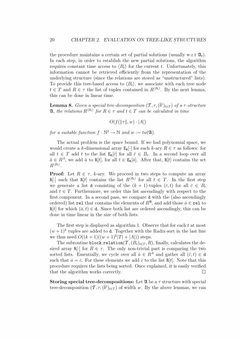
the procedure maintains a certain set of partial solutions (usually w.r.t At).In each step, in order to establish the new partial solutions, the algorithmrequires constant time access to 〈Bt〉 for the current t. Unfortunately, thisinformation cannot be retrieved efficiently from the representation of theunderlying structure (since the relations are stored as “unstructured” lists).To provide this tree-based access to 〈Bt〉, we associate with each tree nodet ∈ T and R ∈ τ the list of tuples contained in R〈Bt〉. By the next lemma,this can be done in linear time.
Lemma 8. Given a special tree-decomposition (T , r, (bt)t∈T ) of a τ -structureA, the relations R〈Bt〉 for R ∈ τ and t ∈ T can be calculated in time
O(f(‖τ‖, w) · |A|)
for a suitable function f : N2 → N and w := tw(A).
The actual problem is the space bound. If we had polynomial space, wewould create a k-dimensional array ER[·] for each k-ary R ∈ τ as follows: forall t ∈ T add t to the list ER[c] for all c ∈ Bt. In a second loop over alla ∈ RA, we add a to R[t], for all t ∈ ER[a]. After that, R[t] contains the setR〈Bt〉.
Proof: Let R ∈ τ , k-ary. We proceed in two steps to compute an arrayR[·] such that R[t] contains the list R〈Bt〉 for all t ∈ T . In the first stepwe generate a list d consisting of the (k + 1)-tuples (c, t) for all c ∈ Bt
and t ∈ T . Furthermore, we order this list ascendingly with respect to thefirst component. In a second pass, we compare d with the (also ascendinglyordered) list rel that contains the elements of RA, and add those a ∈ rel toR[t] for which (a, t) ∈ d. Since both list are ordered ascendingly, this can bedone in time linear in the size of both lists.
The first step is displayed as algorithm 1. Observe that for each t at most(w+ 1)k tuples are added to d. Together with the Radix-sort in the last linewe thus need O((k + 1)((w + 1)k|T |+ |A|)) steps.
The subroutine block relation(T , (Bt)t∈T , R), finally, calculates the de-sired array R[·] for R ∈ τ . The only non-trivial part is comparing the twosorted lists. Essentially, we cycle over all a ∈ RA and gather all (c, t) ∈ d
such that a = c. For these elements we add c to the list R[t]. Note that thisprocedure requires the lists being sorted. Once explained, it is easily verifiedthat the algorithm works correctly. 2
Storing special tree-decompositions: Let A be a τ structure with specialtree-decomposition (T , r, (bt)t∈T ) of width w. By the above lemmas, we can

2.2. COURCELLE’S RESULT AND A SIMPLE EXTENSION 21
1 proc gen ttuples(T , (Bt)t∈T )2 for t ∈ T do3 for c ∈ Bt do append(d, (c, t)) od4 od5 radix sort(d);6 return(d);7 .
Algorithm 1. Generate the list d
compute additional arrays (R[·])R∈τ of size |T | such that for all R ∈ τ andt ∈ T we have:
R[t] = R〈Bt〉 as a linked list.
Observe that since Bt has size (w + 1), each list R[t] for k-ary R has size≤ (w+ 1)k, hence we have the desired constant time decision for queries likea ∈ R〈Bt〉.
2.2 Courcelle’s result and a simple extension
The following theorem is due to Courcelle [Cou90] and states that MSO-properties are linear time decidable over classes of bounded tree-width. Ac-tually, he proved this theorem using context free hyperedge-grammars andclasses definable by equational expressions. We take another way using gamesthat characterize certain fragments of monadic second-order logic (MSO).
Theorem 9. Let w ≥ 1 and ϕ ∈ MSO of quantifier rank q. There is functionf : N2 → N and an algorithm that answers A |= ϕ, for a structure A in time
f(w, q) · ‖A‖
for w := tw(A).
For two structures A,B and q ≥ 0 we write A ≡MSOq B, if A and B
satisfy the same sentences ϕ ∈ MSO of rank ≤ q. ≡MSOq can be charac-
terized by an Ehrenfeucht-Fraisse game that is played by the Spoiler andthe Duplicator. The Spoiler starts choosing one of the two structures, say,A and then decides whether he does a point move or set move. In a point(set) move, the Spoiler chooses some a ∈ A (P ⊆ A), and the Duplicatoranswers b ∈ B (Q ⊆ B). After q moves, elements a1, . . . , ar and subsetsP1, . . . , Ps (q = r + s) in A and corresponding elements b1, . . . , br and sub-sets Q1, . . . , Qs of B have been chosen. Now, the Duplicator has won, if

22 CHAPTER 2. EVALUATION ON TREE-LIKE STRUCTURES
1 proc block relation(T , (Bt)t∈T , R)2 rel := RA;3 d := gen ttuples(T , (Bt)t∈T );4 for a ∈ rel do5 while () do6 (c, t) := current(d);7 if a = c8 then9 append(R[t], a);
10 else11 if predecessor(rel) = c12 then13 break;14 fi15 fi16 next element(d);17 od18 od19 .
Algorithm 2. Calculate R〈Bt〉 for all t ∈ T
a 7→ b ∈ Part((A, P1, . . . , Ps), (B, Q1, . . . , Qs)). The next theorem is folkloreand can be found in, for instance, [EF95].
Theorem 10. A ≡MSOq B iff the Duplicator has a winning strategy for the
q-move game on A and B.
For q ≥ 0 the q-type tpq(A, a) of a k-tuple a ∈ A in a τ -structure A isthe set of all monadic second-order formulas ϕ(x) of quantifier-rank at mostq such that A |= ϕ(a). Using standard techniques, it is easy to see that,up to logical equivalence, there are only finitely many monadic second orderformulas with free variables in x of quantifier rank at most q. Hence tpq(A, a)has a finite description. Observe that (A, a) ≡MSO
q (B, b) is equivalent totpq(A, a) = tpq(B, b).
Since we consider q-types of the substructures At of A, it is convenient tointroduce the shortcuts stype(t) := tpq(At, b
t) and block(t) := (〈Bt〉, bt). Wesay that two blocks corresponding to tree vertices s, t (of maybe different tree-decompositions) are isomorphic (block(s) ∼= block(t)), if there is a bijectivefunction f : Bs → Bt such that for k-ary R ∈ τ and all (a1, . . . , ak) ∈ Bs:a ∈ R〈Bs〉 ⇔ (f(a1), . . . , f(ak)) ∈ R〈Bt〉 and f(bsi ) = bti for all i = 0, . . . , w.

2.2. COURCELLE’S RESULT AND A SIMPLE EXTENSION 23
Remark: When we treat special tree-decompositions, we always use bt todenote the tuple associated with the tree node t ∈ T . Even if we handle var-ious tree-decompositions, this does not introduce ambiguities, if we assumethat different tree-decompositions have disjoint underlying trees T . For con-venience, we still use Bt to denote bt0, . . . , btw; of course only in situationsthat do not depend on the specific ordering of the tuple bt.
For a special tree-decomposition (T , r, (bt)t∈T ), we define the equality-typeat s, t ∈ T as
id(s, t) := (i, j) | 0 ≤ i < j ≤ w, bsi = btj.
The next lemma is essential for Courcelle’s theorem.
Lemma 11. Let A and A′ be τ -structures, and (T , r, (bt)t∈T ) and(T ′, r′, (bt′)t′∈T ′) be special tree-decompositions of A and A′ of widthw ≥ 1, respectively. For t ∈ T and t′ ∈ T ′ with childrenu1, u2 and v1, v2, respectively, the following holds (cf. figure 2.1):If stype(u1) = stype(v1), id(t, u1) = id(t′, v1)and stype(u2) = stype(v2), id(t, u2) = id(t′, v2)and block(t) ∼= block(t′),
then we have stype(t) = stype(t′).
Proof: We prove this lemma using Ehrenfeucht-Fraisse games. Becausetpq(b
u1 ,Au1) = tpq(bv1 ,A′v1
), the Duplicator has a local winning strategy forthe corresponding game on (Au1 , b
u1) and (A′v1, bv1). Likewise he has a local
strategy on (Au2 , bu2) and (Bv2 , b
v2). We have to show that the Duplicatorwins the game on (At, b
t) and (A′t′ , bt′). We show that the Duplicator can
maintain the winning situation. Assume we have a partial isomorphism c 7→ dfrom (At, P , b
t) to (A′t′ , Q, bt′ (this means that P , Q and c, d have already
been pebbled in the game) and that local strategies exist. We show how theDuplicator act in the set moves.
Assume that the Spoiler pebbles a set X ⊆ At. This set splits up intothe parts X1 := X ∩ Au1 and X2 := X ∩ Au2 and X+ := X \ (X1 ∪ X2).According to the local strategies, the Duplicator chooses sets Y1 ⊆ Bu1 , Y2 ⊆Bu2 corresponding to X1, X2. Take Y + to be the image of X+ under theclaimed isomorphism (recall that block(t) and block(t′) are isomorphic). TheDuplicator responds Y := Y1 ∪ Y2 ∪ Y +.
We have to show that c 7→ d is still a partial isomorphism (now of thestructures expanded by X and Y , respectively). Take some a ∈ c1, . . . , cr.Essentially, there are 2 cases: (i) a ∈ bt: then the isomorphism between bt
and bt′
assures that a is mapped to an element a′ with a ∈ X ⇐⇒ a′ ∈ Y .

24 CHAPTER 2. EVALUATION ON TREE-LIKE STRUCTURES
Au1 A′v1
bt′
bt
Au2 A′v2
Figure 2.1: Dependency of types
If (ii) a /∈ bt, then a is contained in, say, Au1 . By the local strategy,according to which the Duplicator chose Y1, we also have a ∈ X1 ⇐⇒ a′ ∈Y1. Observe that we do not have to check for the relation of different a, b ∈c1, . . . , cr, since there conformity with the relations holds by assumption.Since the point moves work similarly, the proof is completed. 2
Let t ∈ T for a special tree-decomposition (T , r, (bt)t∈T ). For each R ∈ τwe define itype(R, t) := (i1, . . . , ik) | (bti1 , . . . , b
tik
) ∈ RA. The isomorphism-type at t ∈ T is the pair
itype(t) := (id(t, t), (R, itype(R, t)) | R ∈ τ).
Observe that itype does not contain any reference to the underlying structureA. It is easy to see that there is an isomorphism between (〈Bt〉, bt) and(〈Bt′〉, bt
′) if, and only if, itype(t) = itype(t′). Then it is an easy corollary of
the last lemma that for t ∈ T with children u1 and u2, stype(t) only dependson stype(u1), stype(u2), itype(t) and how bt and bu1 , and bt and bu2 intersect,respectively. For leaves t, stype(t) only depends on the isomorphism typeof itype(t). This means that there are functions Γ and ∆ such that for allstructures A with an STD (T , r, (bt)t∈T ) of width w we have
stype(t) = Γ(itype(t), stype(u1), id(u1, t), stype(u2), id(u2, t))
for parent nodes t with children u1, u2
stype(t) = ∆(itype(t)) for leaves t.
As already mentioned, there is a finite number of q-types for a fixed q ≥0. Furthermore, the number of different isomorphism types of blocks ofthe decomposition depends only on w. The same holds for the number of

2.2. COURCELLE’S RESULT AND A SIMPLE EXTENSION 25
ways in which adjacent blocks may intersect. Hence, the functions Γ and ∆only depend on w and q, but not on the structure A and can be assumedto be accessible in constant size lookup tables. This thoughts are directlytranslated to the program displayed as algorithm 3. The functions itype(t)and id(s, t) calculate the respective types in constant time by access to thearrays R[·] for R ∈ τ (recall the remark about how tree-decompositions arestored).
1 proc model checkϕ,w(A)2 Compute STD (T , r, (bt)t∈T ) of width w of A
3 tp := stype(r);4 if ϕ ∈ tp then accept else reject fi5 .7 proc stype(t)8 comment: Compute and return stype[t]9 if t is a leaf
10 then stype[t] := (∆(itype(t)))11 else12 u1 := first child of t;13 u2 := second child of t14 stype[t] := Γ(itype(t), stype(u1), id(u1, t),
stype(u2), id(u2, t));15 fi16 return(stype[t]);17 .
Algorithm 3. Checking monadic second-order property ϕ
The correctness of model checkϕ,w follows directly from the properties ofΓ,∆ and the fact that A |= ϕ is equivalent to ϕ ∈ tpq(A, b
r) = stype(r).To estimate the time bound, recall that a STD (T , r, (bt)t∈T ) of A can becomputed in time g(w) · ‖A‖ for some function g.
Because ∆ and Γ are stored in constant size look-up tables and the func-tions itype as well as id need constant time, each recursive call in stype
costs time g′(w, q) for a suitable g′. Summing this up, we obtain a timebound g(w) · ‖A‖+ g′(w, q)|T | = f(w, q) · |A| for some suitable f . 2
2.2.1 Evaluation with one free point variable
Let A be a τ structure. In this section we describe an extension of theresult proved in the last section. In contrast to Courcelle’s algorithm, which

26 CHAPTER 2. EVALUATION ON TREE-LIKE STRUCTURES
only computes tpq(A, br), we now compute (within essentially the same time
bound) tpq(A, bt) for all t ∈ T at once (if T is the underlying tree of a suitable
tree-decomposition). This enables us to associate with each vertex a ∈ A itsq-type tpq(A, a) := ϕ(x) | A |= ϕ(a) and rk(ϕ) ≤ q.
Lemma 12. Let w, q ≥ 0. There is an algorithm that, on input A withtree-width ≤ w, calculates the array tp[a] := tpq(A, a), for all a ∈ A in time
f(w, q) · ‖A‖
for an appropriate f : N2 → N.
Proof: Let (T , r, (bt)t∈T ) be an STD of width w of a τ -structure A. Weadopt the notation from the above discussion. Let t ∈ T . Analogously to At,we define At as the substructure of A “above” t, i.e. At := 〈(A \ At) ∪ Bt〉.The top-type is ttype(t) := tpq(A
t, bt) and we define type(t) := tpq(A, bt).
Our goal is to compute type(t) for all t ∈ T , since from that we caneasily extract the desired information. For a = bti, we get tpq(A, a) =ϕ(xi) | ϕ(xi) ∈ type(t), hence we can concentrate on type(t) for all t ∈ T .Observe that for all t ∈ T we have (cf. figure 2.2)
At
At
bt bt bt
bt
At At
Figure 2.2: Computing type(t).
type(t) = Γ(itype(t), stype(t), id(t, t), ttype(t), id(t, t)).
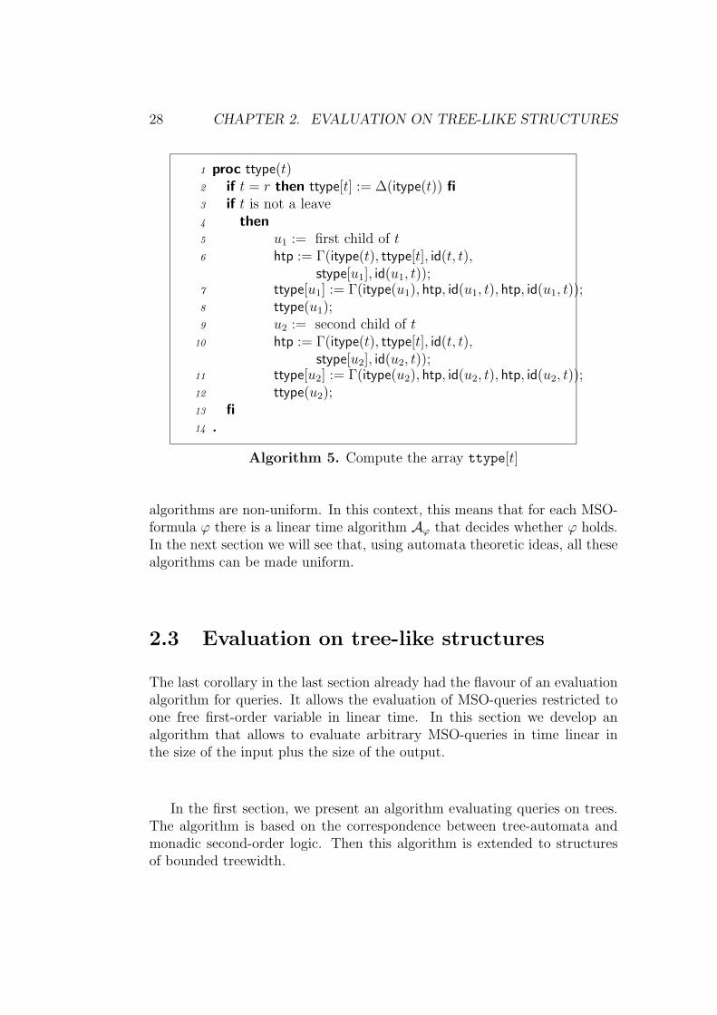
Hence we are done, if we know stype(t) and ttype(t) for all t ∈ T . The arraystype[·] is computed (bottom-up) by the subroutine stype(r) from the proofof Courcelle’s theorem. For the computation of ttype[t] for t ∈ T observethe following:Let t be a node, t 6= r with parent s and sibling t′. Observe that
tpq(〈At′ ∪ As〉, bs) = Γ(itype(s), ttype(s), id(s, s), stype(t′), id(t′, s)).

2.2. COURCELLE’S RESULT AND A SIMPLE EXTENSION 27
If we denote this type with τ we get
ttype(t) = Γ(itype(t), τ, id(s, t), τ, id(s, t)).
The straightforward implementation is displayed as algorithms 4 and 5. Aftercomputing the STD of A we compute the two arrays stype and ttype asexplained above. Then an easy loop over all vertices t ∈ T associates witht the corresponding type type(t). This proves the correctness. For the timebound notice that each of the first two calls take time linear in |A|. Thesame holds for last loop. 2
1 proc model checkϕ,w(A)2 Compute STD (T , r, (bt)t∈T ) of width w of A
3 stype(r); ttype(r);4 for t ∈ T do5 type[t] := Γ(itype(t), stype[t], id(t, t),
ttype[t], id(t, t));6 for i = 0 to w do7 if tp[bti] 6= NULL8 then9 tp[bti] := ϕ(xi) | ϕ(xi) ∈ type[t]
10 fi11 od12 od13 .
Algorithm 4. Compute type[a] for all a ∈ A
The following lemma will be needed in the next chapter.
Corollary 13. Let w ≥ 1 and ϕ(x) ∈ MSO of quantifier rank q. There isa function f : N2 → N and an algorithm that on input A calculates the seta ∈ A | A |= ϕ(a) in time
f(w, q) · ‖A‖.
Proof: In a first step we associate tpq(A, a) with each vertex a ∈ A (throughthe array tp in the last lemma). Then we perform a loop over all a ∈ A andadd those a to the set, for which ϕ(x) ∈ tp[a]. 2
Remark: Note that these model-checking algorithms require the functionsΓ and ∆. Since we did not explain how their tables can be computed, our
28 CHAPTER 2. EVALUATION ON TREE-LIKE STRUCTURES
1 proc ttype(t)2 if t = r then ttype[t] := ∆(itype(t)) fi3 if t is not a leave4 then5 u1 := first child of t6 htp := Γ(itype(t), ttype[t], id(t, t),
stype[u1], id(u1, t));7 ttype[u1] := Γ(itype(u1), htp, id(u1, t), htp, id(u1, t));8 ttype(u1);9 u2 := second child of t
10 htp := Γ(itype(t), ttype[t], id(t, t),stype[u2], id(u2, t));
11 ttype[u2] := Γ(itype(u2), htp, id(u2, t), htp, id(u2, t));12 ttype(u2);13 fi14 .
Algorithm 5. Compute the array ttype[t]
algorithms are non-uniform. In this context, this means that for each MSO-formula ϕ there is a linear time algorithm Aϕ that decides whether ϕ holds.In the next section we will see that, using automata theoretic ideas, all thesealgorithms can be made uniform.
2.3 Evaluation on tree-like structures
The last corollary in the last section already had the flavour of an evaluationalgorithm for queries. It allows the evaluation of MSO-queries restricted toone free first-order variable in linear time. In this section we develop analgorithm that allows to evaluate arbitrary MSO-queries in time linear inthe size of the input plus the size of the output.
In the first section, we present an algorithm evaluating queries on trees.The algorithm is based on the correspondence between tree-automata andmonadic second-order logic. Then this algorithm is extended to structuresof bounded treewidth.

2.3. EVALUATION ON TREE-LIKE STRUCTURES 29
2.3.1 Evaluating MSO-queries on colored trees
Before we start, we need to introduce the basic concepts concerning treeautomata. Let Γ be a finite alphabet. We define τΓ to be the vocabularyconsisting of a binary relation symbol E, a constant r and an unary relationsymbol Pγ for each γ ∈ Γ. A Γ-tree is a τΓ-structure whose underlying graph(the reduction to E) is a binary tree rooted in r and the Pγ for γ ∈ Γ forma partition of the universe. A colored tree is a Γ-tree for some Γ. We say thata vertex t of a colored tree T has color γ, if t ∈ P Tγ . In this case we writeγ(t) = γ.
A (bottom-up) Γ-tree automaton is a 4-tuple A = (Q, δ,∆, F ), where Qis the finite set of states and ∆ : Γ→ Q the starting function. F ⊆ Q is theset of accepting states and δ : Pow≤2(Q)× Γ→ Q is the transition function.
The run (observe that δ is a function) ρ : T → Q of A on the Γ-tree T isdefined in a bottom-up manner. If t is a leaf, then ρ(t) := ∆(γ(t)). If t haschildren s1, s2 then ρ(t) := δ(ρ(s1), ρ(s2), γ(t)). The automaton A is saidto accept T if ρ(rT ) ∈ F . Otherwise we say that A rejects T .
A class of colored trees is recognizable, if it is the class of trees acceptedby some tree-automaton.
Theorem 14 (Thatcher and Wright [TW68, Tho97]). Let Γ be a finitealphabet. A class of Γ-trees is recognizable, if and only if, it is definable byan MSO[τΓ] sentence.
We proceed as follows: since the above theorem only applies to sen-tences we show how formulas with free variables have to be treated. First,we replace free first-order variables by free second-order variables. Thenwe show how free second-order variables correspond to an extension ofthe vocabulary on the automaton side. So assume that we have givenan MSO-formula ϕ(X1, . . . , Xl, y1, . . . , ym). We translate ϕ to a formulaϕ′(X1, . . . , Xl, Y1, . . . , Ym) such that for every structure A and B, C ⊆ A
A |= ϕ′(B, C) ⇔ there are c1, . . . , cm ∈ A with C1 = c1, . . . , Cm = cmand A |= ϕ(B, c)
Now let be given ϕ(X1, . . . , Xk) ∈ MSO[τΓ] for an alphabet Γ and a Γ-treeT . To code assignments of the free variables Xi into the tree, we extend thealphabet to Γ′ := Γ×0, 1k. Then, given an assignment B1, . . . , Bk ⊆ T forour free variables, we obtain the corresponding Γ′-tree T ′ := (T ; B1, . . . , Bk)by the obvious expansion of the vocabulary. In particular, if γ(t) denotes thecolor of t in T , we define
γ′(t) = (γ, ε) ⇔ γ(t) = γ and (t ∈ Bi ⇔ εi = 1) for i = 1, . . . , k.

30 CHAPTER 2. EVALUATION ON TREE-LIKE STRUCTURES
The tuple ε is called the additional color of t. This establishes the corre-spondence between assignments on the one side and colors on the other.Observe that (T ; B1, . . . , Bk) does not denote the expansion of T with knew unary relations (this is why we use a semicolon instead of a comma).In fact, (T ; B1, . . . , Bk) denotes the τΓ′-structure (T,ET , (P T
(γ,ε))γ∈Γ,ε∈0,1k),
where P(γ,ε) is defined above (cf. the definition of γ′).It is easy to see that the class
(T ; B) | T a colored Γ-tree, B ∈ ϕ(T )
is axiomatized by the τΓ′-sentence
ϕ′ := ∃X1 . . . Xk∃(Yγ)γ∈Γ
(ϕ(X)∧
∀t( ∧γ∈Γ
∧ε∈0,1k
(P(γ,εi)t↔ (Yγt ∧∧i:εi=1
Xit ∧∧i:εi=0
¬Xit)))).
where ϕ(X) is obtained from ϕ(X) by replacing all Pγ with the unary second-order variable Yγ, and using ∃(Yγ)γ∈Γ as a shortcut for the existential quan-tification of all Yγ, γ ∈ Γ. As it will turn out, this characterization sufficesto apply theorem 14 to our problem. Let us state our main theorem for thecase of Γ-trees.
Theorem 15. There exists a function f and an algorithm that solves theevaluation problem for MSO-formulas on colored trees in time
f(‖ϕ‖) · (‖T ‖+ ‖ϕ(T )‖)
on input ϕ(X1, . . . , Xl, x1, . . . , xm) and T .
Proof: By the discussion above, we assume the input consisting of a formulaof the form ϕ(X1, . . . , Xk) ∈ MSO[τΓ] and a Γ-tree T . Remember that theclass C is defined by the above MSO[τΓ′ ]-sentence ϕ′. Hence, there is a Γ′-automaton A = (Q,∆, δ, F ) recognizing C.
Now we get an easy and constructive characterization of the sought set.For the input Γ-tree T we have
ϕ(T ) = B | A accepts (T ; B).
This gives us the idea for the algorithm. We simply collect the additionalcolors such that A accepts T expanded by those colors. The presentationof the algorithm (doing this in an optimal way) involves two parts. In thefirst part, we describe how the algorithm is going to work, including the

2.3. EVALUATION ON TREE-LIKE STRUCTURES 31
correctness of the steps performed by the algorithm. In a second part, wegive a detailed implementation of the algorithm together with an analysis ofthe running time and the data structures involved.
I.) The algorithm: We pass through the tree T three times. In a firstbottom-up pass we collect the set of states that could be reached by theautomaton. Then we go down, sorting out those states that do not lead toaccepting states, and finally we go bottom-up again gathering the satisfyingassignments for ϕ(X) (even considering only those).
1. Bottom-up: By induction from the leaves to the root, we first compute,for every t ∈ T , a set Pt of “potential states” at t: If t is a leaf, thenPt := ∆((γ(t), ε)) | ε ∈ 0, 1k. For an inner vertex t with children s1 ands2, we set
Pt := δ(q1, q2, (γ(t), ε)) | q1 ∈ Ps1 , q2 ∈ Ps2 , ε ∈ 0, 1k.
Then for all t ∈ T and q ∈ Q we have q ∈ Pt if, and only if, there are setsB1, . . . , Bk ⊆ T such that for the run ρ of A on (T ; B) we have ρ(t) = q.This is easily proved by induction.
Note that if Pr ∩ F = ∅ we have ϕ(T ) = ∅, and no further action isrequired.
2. Top-down: Starting at the root r := rT we compute, for every t ∈ T ,the subset St of Pt of “success states” at t: We let Sr := F ∩ Pr. If t hasparent s and sibling t′, then
St := q ∈ Pt | there are q′ ∈ Pt′ , ε ∈ 0, 1k such that δ(q, q′, (γ(s), ε)) ∈ Ss.
Then for all t ∈ T and q ∈ Q we have q ∈ St if, and only if, there are setsB1, . . . , Bk ⊆ T such that A accepts (T , B) and for the run ρ of A on (T , B)we have ρ(t) = q (again easy by induction).
3. Bottom-up again: Recall that for t ∈ T , by Tt we denote the subtreeof T rooted in t. For t ∈ T and q ∈ St we let
Satt,q :=B ⊆ Tt
There are sets B′1, . . . , B′k ⊆ T such that
B′i ∩ Tt = Bi for 1 ≤ i ≤ k,A accepts (T , B′),and for the run ρ of A on (T , B′) we haveρ(t) = q
.
We compute the sets Satt,q inductively from the leaves to the root. Let t ∈ Tand q ∈ St. Set Bt
1 := t and Bt0 = ∅. If t is a leaf, then
Satt,q = (Btε1, . . . , Bt
εk) | ∆((γ(t), ε)) = q.
32 CHAPTER 2. EVALUATION ON TREE-LIKE STRUCTURES
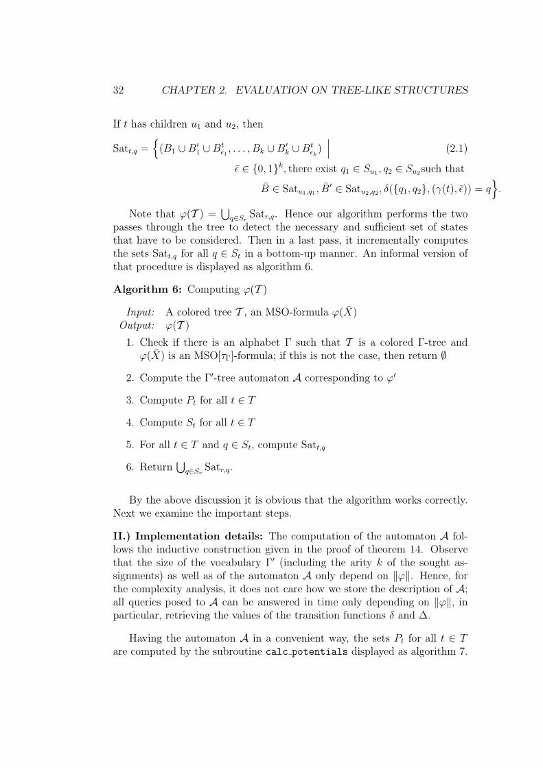
If t has children u1 and u2, then
Satt,q =
(B1 ∪B′1 ∪Btε1, . . . , Bk ∪B′k ∪Bt
εk) (2.1)
ε ∈ 0, 1k, there exist q1 ∈ Su1 , q2 ∈ Su2such that
B ∈ Satu1,q1 , B′ ∈ Satu2,q2 , δ(q1, q2, (γ(t), ε)) = q
.
Note that ϕ(T ) =⋃q∈Sr Satr,q. Hence our algorithm performs the two
passes through the tree to detect the necessary and sufficient set of statesthat have to be considered. Then in a last pass, it incrementally computesthe sets Satt,q for all q ∈ St in a bottom-up manner. An informal version ofthat procedure is displayed as algorithm 6.
Algorithm 6: Computing ϕ(T )
Input: A colored tree T , an MSO-formula ϕ(X)Output: ϕ(T )
1. Check if there is an alphabet Γ such that T is a colored Γ-tree andϕ(X) is an MSO[τΓ]-formula; if this is not the case, then return ∅
2. Compute the Γ′-tree automaton A corresponding to ϕ′
3. Compute Pt for all t ∈ T
4. Compute St for all t ∈ T
5. For all t ∈ T and q ∈ St, compute Satt,q
6. Return⋃q∈Sr Satr,q.
By the above discussion it is obvious that the algorithm works correctly.Next we examine the important steps.
II.) Implementation details: The computation of the automaton A fol-lows the inductive construction given in the proof of theorem 14. Observethat the size of the vocabulary Γ′ (including the arity k of the sought as-signments) as well as of the automaton A only depend on ‖ϕ‖. Hence, forthe complexity analysis, it does not care how we store the description of A;all queries posed to A can be answered in time only depending on ‖ϕ‖, inparticular, retrieving the values of the transition functions δ and ∆.
Having the automaton A in a convenient way, the sets Pt for all t ∈ Tare computed by the subroutine calc potentials displayed as algorithm 7.

2.3. EVALUATION ON TREE-LIKE STRUCTURES 33
The call of calc potentials(r) provides the set Pt as array element p[t] forall t ∈ T . For that, we recursively descent the tree and compute Pt by adirect evaluation of the definition. Note that the colors of tree vertices t ∈ Tare stored in an array over T (cf. the appendix on page 110). This admitsaccess to γ(t) in time h(‖Γ′‖) for a suitable h. Since we also have constanttime access to δ and ∆, we can evaluate the definition of Pt (in each levelt ∈ T ) in time f(‖ϕ‖) for some function f .
1 proc calc potentials(t)2 if t is a leaf3 then4 p[t] := ∆((γ(t), ε) | ε ∈ 0, 1k5 else6 u1 := first child of t7 u2 := second child of t8 calc potentials(u1); calc potentials(u2);9 p[t] := δ(q1, q2, (γ(t), ε)) | q1 ∈ p[s1],
q2 ∈ p[s2], ε ∈ 0, 1k10 fi11 .
Algorithm 7. Compute the sets Pt for t ∈ T
Together, the time for the entire procedure call sums up to f(‖ϕ‖) · |T |.The subroutine calc successfuls works like calc potentials, implement-ing the above recursive procedure for the sets St (there we fill up the arrays[·]). Thus, steps 3 and 4 need time f(‖ϕ‖) · |T | each.
Step 5 is the crucial one, and to compute the sets Satt,q we have toproceed particularly carefully to obtain the optimal time bound claimed inthe theorem. We shall use the following two facts about the sets Satt,q.
(1) Satt,q is non-empty for all t ∈ T and q ∈ St
(2) Satt,q ∩ Satt,q′ = ∅ for all t ∈ T , q, q′ ∈ St such that q 6= q′
The first one claims that all sets Satt,q that are sufficient for the compu-tation of ϕ(T ) are actually necessary, while the second essentially says thatno tuple is handled twice.
Proof: (of the two claims) For the first claim assume q ∈ St. By definition,this is equivalent to there exists a B such that for the accepting run ρ of A

34 CHAPTER 2. EVALUATION ON TREE-LIKE STRUCTURES
on (T , B) we have ρ(t) = q; hence B ∩ Tt ∈ Satt,q. The second claim followsfrom the fact that A is deterministic, i.e. different states in t ∈ T can onlybe reached in runs over different colorings. 2
By definition, Satt,q contains sets of k-tuples of subsets of the universeT (the assignments for X1, . . . , Xk). To represent these sets we use a datastructure of the following form: subsets of the universe T are stored as linkedlists (cf. section A.3). Then a k-tuple A is represented as a k-size array suchthat the ith array element is a pointer to the list Ai. The arrays A themselves,are again arranged as lists (cf. the distinction between big and small datastructures in the appendix).
Let T ′, T ′′ be disjoint sets and S ′, S ′′ two non-empty sets of k-tuples ofsubsets of T ′ and T ′′, respectively. The operation required to compute Satt,q(cf. the definition) corresponds to
merge(S ′, S ′′) := (B′1 ∪B′′1 , . . . , B′k ∪B′′k) | B′ ∈ S ′, B′′ ∈ S ′′,
whose implementation is displayed as algorithm 8. Note that this is a socalled destructive procedure, since after the call the arguments are part of theresult.
Let us estimate the time needed by algorithm 8 to merge the sets s′, s′′.Apart from the if-statements at the beginning of the code, we perform aloop over all tuples assign′ ∈ s′, assign′′ ∈ s′′ and concatenate each ofthem componentwise. This concatenation is done in constant time (cf. theappendix). As mentioned above, we incorporate the arguments into theresult. This is guaranteed by the two if-clauses, e.g. the first one assures thateach but the last entry of s′ is concatenated with a copy of the respectiveassign′′ ∈ s′′. On the other hand, the elements assign′′ ∈ s′′ (themselves)are concatenated with the last entry of s′. The second if-clause does thesame with reversed roles of assign′ and assign′′. Hence, all elements of s′
and s′′ are reused.
Making a copy of an object x takes time ‖x‖. Hence, altogether we needtime
O(1 + |merge(s′, s′′)|+ ‖merge(s′, s′′)‖ − ‖s′‖ − ‖s′′‖)
to compute the merge of two sets s′, s′′. Note here that |s| stands for thenumber of items contained in the list s, while ‖s‖ :=
∑(B1,...,Bk)∈s
∑ki=1 |Bi|.
Two get a more convenient representation of this upper bound, we use furtherconditions that are assured by the three if-clauses (i.e. s′, s′′ 6= ∅ and s′, s′′ 6=(∅, . . . , ∅)) at the beginning of the procedure. Under these conditions we

2.3. EVALUATION ON TREE-LIKE STRUCTURES 35
1 proc merge(s’, s”)2 ms := ∅; /* the merged set */3 if empty(s’) or empty(s”) then return(ms) fi;4 if s’ = (∅, . . . , ∅) then return(s”) fi;5 if s” = (∅, . . . , ∅) then return(s’) fi;6 for assign’ ∈ s’ do7 for assign” ∈ s” do8 if last(s’, assign’)9 then a2 := assign”
10 else a2 := copy(assign”)11 fi12 if last(s”, assign”)13 then a1 := assign’14 else a1 := copy(assign’)15 fi16 for i = 1 to k do /* concatenate the sets */17 append(a1[i], a2[i]);18 od19 append(ms, a1); /* add it to the result */20 od21 od22 return(ms);23 .
Algorithm 8. Destructively merging two sets of assignments
can show that
O(1 + |merge(s′, s′′)|+ ‖merge(s′, s′′)‖ − ‖s′‖ − ‖s′′‖)= O(1 + ‖merge(s′, s′′)‖ − ‖s′‖ − ‖s′′‖), (2.2)
which simplifies the subsequent analysis of the main algorithm. To provethis, assume w.l.o.g. that |s′| ≥ |s′′| and that |s′| is sufficiently big (otherwise(2.2) holds trivially). If |s′′| = 1 then ‖merge(s′, s′′)‖ = |s′| · ‖s′′‖ + ‖s′‖,hence ‖merge(s′, s′′)‖ − ‖s′‖ − ‖s′′‖ ≥ |s′| − 1 (since ‖s′′‖ ≥ 1). Togetherwith |merge(s′, s′′)| = |s′|, this implies equation (2.2) for this case.
If |s′′| > 1, then ‖merge(s′, s′′)‖ − ‖s′‖ − ‖s′′‖ ≥ |merge(s′, s′′)|. Hence,as before, we obtain (2.2).
Having proved an upper bounded for algorithm 8, let us move to the mainalgorithm. Given a t ∈ T , algorithm 9 computes the sets Satt,q for all q ∈ St.

36 CHAPTER 2. EVALUATION ON TREE-LIKE STRUCTURES
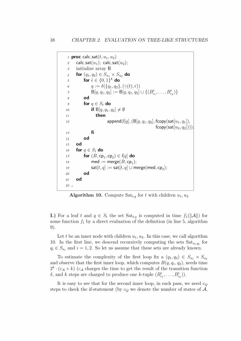
The case where t is a leaf is handled in the loop around line 5. Its correctnessis obvious. For inner nodes we call the procedure calc sat(t, u1, u2) displayedas algorithm 10, where u1, u2 are the children of t.
1 proc calc sat(t)2 if t is a leaf3 then4 for q ∈ St do5 sat[t, q] := (Bt
ε1, . . . , Bt
εk) | ∆((γ(t), ε)) = q
6 od7 else8 u1 := first child of t;9 u2 := second child of t;
10 calc sat(t, u1, u2);11 fi12 .
Algorithm 9. Calculate Satt,q for all q ∈ St
Now consider algorithm 10. In the second line we compute the valuesSatui,qi for qi ∈ Sui , i = 1, 2. Based on these values we want to computeSatt,q for q ∈ St in an efficient way (reusing all already obtained partialassignments). We explain the functionality in two phases: first, we describewhy we get the right answer and second, we give a detailed account on therunning time of the procedure.
Essentially, the procedure consists of two loops. In the first one (lines 4 to15), we prepare for the second one (lines 16 to 21), which actually computesthe desired sets by means of merges. To understand the first loop, take apair (q1, q2) ∈ Su1 × Su2 , a q ∈ St and define
B(q, q1, q2) := (Btε1, . . . , Bt
εk) | δ(q1, q2, (γ(t), ε)) = q.
The first inner loop computes this set B[q, q1, q2], which intuitively con-tains the tuples by which assignments from Satu1,q1 and Satu2,q2 extend toassignments in Satt,q. For the second inner loop (around the if-clause in line10) we need to have a closer look at the problem of reusing intermediateresults.
Our objective is to compute the sets Satt,q, which in terms of the merge-function can be characterized as the following disjoint union:
Satt,q =⋃
(q1,q2)∈Su1×Su2B(q,q1,q2) 6=∅
merge(merge(Satu1,q1 , B(q, q1, q2)), Satu2,q2). (*)

2.3. EVALUATION ON TREE-LIKE STRUCTURES 37
In a straightforward implementation, we would simply merge all setsSatu1,q1 , B(q, q1, q2), and Satu2,q2 with B(q, q1, q2) 6= ∅. Recall here that mergeis destructive, i.e. after the call of merge(s′, s′′) the parameters s′, s′′ are nolonger available (they have become part of the result). On the other hand,we cannot copy each argument before passing it to the merge-procedure; thiswould be to wasteful.
Our solution to this problem is to make copies of all Satu1,q1 and Satu2,q2
that are to be merged with some B(q, q1, q2) (one copy for each subsequentapplication of (*)). When doing the copies, we guarantee at the same timethat we only make a copy, if it is really necessary. This allows direct calls ofthe merge-procedure in the subsequent loop and, as we will see, assures theclaimed time bound.
To avoid unhandy pre-estimations of the number of copies that have tobe made, we enhance the data structure for the sets Satt,q by a “usage”-flag,which indicates, if the set has already been copied. Initially, after the objectis created, this flag is set “off”. In this context we introduce the functionfcopy(x) which first looks if the flag of x is “on”, and if so, returns a copyof x. If the flag is “off”, the flag is flipped “on” and x itself is returned.
So we come back to the second inner loop: for each non-empty B(q, q1, q2)we store the triple (Satu1,q1 , Satu2,q2 , B(q, q1, q2)) in the list l[q]. And theseare exactly the arguments of the merges of the form (*) that have to be doneto obtain Satt,q for all q ∈ St.
In the second outer loop (lines 16 to 21), we finally generate the setsSatt,q from the elements of the list l[q]. This proves the correctness of thealgorithm.
The running time: We will show by induction over t ∈ T that all Satt,q,q ∈ St are computed in time
T (t) ≤ c ·∑q∈St
‖Satt,q‖+ f(‖A‖) · |Tt|
for a constant c and a suitable function f (these will be defined later). Thenthe theorem follows with property (2) of Satt,q. To prove this bound, we firstgive a recursive characterization of the time algorithm 9 spends at a nodet ∈ T . In a second step, we show inductively that this recursive formulayields the upper bound claimed above.
38 CHAPTER 2. EVALUATION ON TREE-LIKE STRUCTURES
1 proc calc sat(t, u1, u2)2 calc sat(u1); calc sat(u2);3 initialize array B4 for (q1, q2) ∈ Su1 × Su2 do5 for ε ∈ 0, 1k do6 q := δ(q1, q2, (γ(t), ε))7 B[q, q1, q2] := B[q, q1, q2] ∪ (Bt
ε1, . . . , Bt
εk)
8 od9 for q ∈ St do
10 if B[q, q1, q2] 6= ∅11 then12 append(l[q], (B[q, q1, q2], fcopy(sat[u1, q1]),
fcopy(sat[u2, q2])));13 fi14 od15 od16 for q ∈ St do17 for (B, cp1, cp2) ∈ l[q] do18 med := merge(B, cp1);19 sat[t, q] := sat[t, q] ∪merge(med, cp2);20 od21 od22 .
Algorithm 10. Compute Satt,q for t with children u1, u2
I.) For a leaf t and q ∈ St the set Satt,q is computed in time f1(‖A‖) forsome function f1 by a direct evaluation of the definition (in line 5, algorithm9).
Let t be an inner node with children u1, u2. In this case, we call algorithm10. In the first line, we descend recursively computing the sets Satui,qi forqi ∈ Sui and i = 1, 2. So let us assume that these sets are already known.
To estimate the complexity of the first loop fix a (q1, q2) ∈ Su1 × Su2
and observe that the first inner loop, which computes B(q, q1, q2), needs time2k · (cA + k) (cA charges the time to get the result of the transition functionδ, and k steps are charged to produce one k-tuple (Bt
ε1, . . . , Bt
εk)).
It is easy to see that for the second inner loop, in each pass, we need cQsteps to check the if-statement (by cQ we denote the number of states of A,

2.3. EVALUATION ON TREE-LIKE STRUCTURES 39
i.e. cQ := |Q|). Furthermore, for all (q1, q2) together, we need
c1·(∑q∈St
∑(q1,q2),
B(q,q1,q2) 6=∅
(‖Satu1,q1‖+‖Satu2,q2‖
)−∑q1∈Su1
‖Satu1,q1‖−∑q2∈Su2
‖Satu2,q2‖)
steps to do the copies. In particular, the first double sum accounts forthe effort to make the copies (in line 12). From this cost we have to subtractthe work we saved by reusing the sets Satui,qi , qi ∈ Sui . The constant c1
takes care for the overhead produced by fcopy and the generation of l[q](this constant is independent from T and A). Hence, we need
c2Q · 2k · (cA + k) + c3
Q + c1 ·∑q∈St
∑(q1,q2),
B(q,q1,q2) 6=∅
(‖Satu1,q1‖+ ‖Satu2,q2‖
)− c1 ·
( ∑q1∈Su1
‖Satu1,q1‖+∑q2∈Su2
‖Satu2,q2‖)
steps for the entire first loop (in the sequel, we denote the term c2Q · 2k ·
(cA + k) + c3Q by f(‖A‖)).
The second loop simply merges all of the recently computed sets. Theneeded time sums up to
c2 ·∑q∈St
∑(q1,q2),
B(q,q1,q2) 6=∅
(‖merge(merge(Satu1,q1 , B(q, q1, q2)), Satu2,q2)‖
− ‖Satu1,q1‖ − ‖B(q, q1, q2)‖ − ‖Satu2,q2‖),
where c2 is the constant from the merge-function. Observe that we donot need to account for the loops, since there are no void loops (property(1) above). In characterization (*) of Satt,q the union is disjoint, hence, thisvalue is dominated by
c2 ·(∑q∈St
‖Satt,q‖ −∑q∈St
∑(q1,q2),
B(q,q1,q2) 6=∅
(‖Satu1,q1‖+ ‖Satu2,q2‖
)).
Altogether, it is obvious that for the time T (t) spent at an inner node t ∈ T

40 CHAPTER 2. EVALUATION ON TREE-LIKE STRUCTURES
with children u1, u2 we have
T (t) ≤ T (u1) + T (u2) + f(‖A‖)
+ (c1 − c2) ·∑q∈St
∑(q1,q2),
B(q,q1,q2) 6=∅
(‖Satu1,q1‖+ ‖Satu2,q2‖
)
− c1 ·( ∑q1∈Su1
‖Satu1,q1‖+∑q2∈Su2
‖Satu2,q2‖)
+ c2 ·∑q∈St
‖Satt,q‖.
II.) It remains to prove that this recursion formula yields the claimed upperbound. Define c := c1 + c2. By induction hypothesis, T (ui) ≤ f(‖A‖) ·|Tui| + c ·
∑qi∈Sui
‖Satui,qi‖ for i = 1, 2. If we insert this into the recursive
characterization of T (t), we get T (t) ≤ f(‖A‖) · (|Tu1|+ |Tu2|+ 1)
+ (c1 + c2) ·( ∑q1∈Su1
‖Satu1,q1‖+∑q2∈Su2
‖Satu2,q2‖)
+ (c1 − c2) ·∑q∈St
∑(q1,q2),
B(q,q1,q2) 6=∅
(‖Satu1,q1‖+ ‖Satu2,q2‖
)
− c1 ·( ∑q1∈Su1
‖Satu1,q1‖+∑q2∈Su2
‖Satu2,q2‖)
+ c2 ·∑q∈St
‖Satt,q‖,
which is equal to
f(‖A‖) · |Tt|+ c2 ·∑q∈St
‖Satt,q‖
+ (c1 − c2) ·∑q∈St
∑(q1,q2),
B(q,q1,q2) 6=∅
(‖Satu1,q1‖+ ‖Satu2,q2‖
)
+ c2 ·( ∑q1∈Su1
‖Satu1,q1‖+∑q2∈Su2
‖Satu2,q2‖).
It is easy to see that
∑q∈St
∑(q1,q2),
B(q,q1,q2) 6=∅
(‖Satu1,q1‖+ ‖Satu2,q2‖
)≤∑q∈St
‖Satt,q‖,

2.3. EVALUATION ON TREE-LIKE STRUCTURES 41
hence, we have
T (t) ≤ f(‖A‖) · |Tt|+ (c1 + c2) ·∑q∈St
‖Satt,q‖
+ c2 ·(( ∑
q1∈Su1
‖Satu1,q1‖+∑q2∈Su2
‖Satu2,q2‖)
−∑q∈St
∑(q1,q2),
B(q,q1,q2) 6=∅
(‖Satu1,q1‖+ ‖Satu2,q2‖
)),
which is smaller than f(‖A‖) · |Tt| + c ·∑
q∈St ‖Satt,q‖ (since the lastaddend is ≤ 0). As mentioned in the beginning of the complexity analysis,this bound on T (t) completes the proof of theorem 15. 2
We immediately get the following corollary.
Corollary 16. There exists a function f and an algorithm that solves theevaluation problem for MSO-formulas with no free set variables on coloredtrees in time
f(‖ϕ‖) · (‖T ‖+ |ϕ(T )|)on input ϕ(x1, . . . , xk) and T .
Proof: For a formula without free set variables we have ‖ϕ(T )‖ = k ·|ϕ(T )| ≤ ‖ϕ‖ · |ϕ(T )| (since all variables xi must occur freely in ϕ(x)). 2
The witness case for MSO on colored trees is now an easy corollary oftheorem 15.
Corollary 17. There exists a function f and an algorithm that solves thewitness problem for MSO-formulas on colored trees in time
f(‖ϕ‖) · ‖T ‖
on input ϕ(X1, . . . , Xl, x1, . . . , xm) and T .
Proof: Proceed as before, until the calculation of Satt,q. Now we select anaccepting run ρ : T → Q on T and then compute a particular coloring of Tinducing that run. We start with an arbitrary q ∈ Sr and proceed top-down.Assume that in node t we are in state q ∈ St and t has children u1, u2. Nowchoose an additional color εt ∈ 0, 1k and states q1 ∈ Su1 and q2 ∈ Su2
such that δ(q1, q2, (γ(t), εt)) = q. If t is a leaf and ρ(t) = q, choose anεt ∈ 0, 1k such that ∆((γ(t), εt)) = q. The tuple A = (A1, . . . , Ak) withAi := t | εti = 1 is an satisfying assignment. The analysis is straightforwardand omitted. 2
42 CHAPTER 2. EVALUATION ON TREE-LIKE STRUCTURES
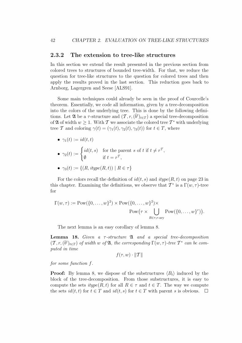
2.3.2 The extension to tree-like structures
In this section we extend the result presented in the previous section fromcolored trees to structures of bounded tree-width. For that, we reduce thequestion for tree-like structures to the question for colored trees and thenapply the results proved in the last section. This reduction goes back toArnborg, Lagergren and Seese [ALS91].
Some main techniques could already be seen in the proof of Courcelle’stheorem. Essentially, we code all information, given by a tree-decompositioninto the colors of the underlying tree. This is done by the following defini-tions. Let A be a τ -structure and (T , r, (bt)t∈T ) a special tree-decompositionof A of width w ≥ 1. With T we associate the colored tree T ∗ with underlyingtree T and coloring γ(t) = (γ1(t), γ2(t), γ3(t)) for t ∈ T , where
• γ1(t) := id(t, t)
• γ2(t) :=
id(t, s) for the parent s of t if t 6= rT ,
∅ if t = rT ,
• γ3(t) := (R, itype(R, t)) | R ∈ τ
For the colors recall the definition of id(t, s) and itype(R, t) on page 23 inthis chapter. Examining the definitions, we observe that T ∗ is a Γ(w, τ)-treefor
Γ(w, τ) := Pow(0, . . . , w2)× Pow(0, . . . , w2)×
Pow(τ ×
⋃R∈τ,r-ary
Pow(0, . . . , wr)).
The next lemma is an easy corollary of lemma 8.
Lemma 18. Given a τ -structure A and a special tree-decomposition(T , r, (bt)t∈T ) of width w of A, the corresponding Γ(w, τ)-tree T ∗ can be com-puted in time
f(τ, w) · ‖T ‖
for some function f .
Proof: By lemma 8, we dispose of the substructures 〈Bt〉 induced by theblock of the tree-decomposition. From those substructures, it is easy tocompute the sets itype(R, t) for all R ∈ τ and t ∈ T . The way we computethe sets id(t, t) for t ∈ T and id(t, s) for t ∈ T with parent s is obvious. 2

2.3. EVALUATION ON TREE-LIKE STRUCTURES 43
T ∗ does not contain any reference to the structure A, hence the problemarises of how to “speak” about subsets and elements of A in the colored treeT ∗. Thereto, we code each element a ∈ A by a canonical tuple of subsets ofT . This tuple defines a unique (t, i) such that a = bti.
For an element a ∈ A we let node(a) be the minimal t ∈ T with respectto ≤T such that a ∈ bt0, . . . , btw. We define U(a) := (U1(a), . . . , Uw(a)) by
Ui(a) :=
node(a) if b
node(a)i = a and b
node(a)j 6= a for 1 ≤ j < i,
∅ otherwise,
for 0 ≤ i ≤ w. This tuple is a unique representative for the element a: itencodes in which bt the element a occurs first (w.r.t ≤T ), and its minimalplace (w.r.t. the ordered tuple) in the tuple bt. For a subset B ⊆ A welet Ui(B) :=
⋃a∈B Ui(a) and U(B) := (U0(B), . . . , Uw(B)). Note that for
subsets U0, . . . , Uw ⊆ T there exists an a ∈ A such that U = U(a) if, andonly if,
(1)⋃wi=0 Ui is a singleton.
(2) For all t ∈ T and 0 ≤ i < j ≤ w: If t ∈ Uj then (i, j) /∈ γ1(t).
(3) For all t ∈ T , t 6= rT , with parent s and 0 ≤ i, j ≤ w: If t ∈ Ui then(i, j) /∈ γ2(t).
Moreover, there is a subset B ⊆ A with U = U(B) just in case theconditions (2) and (3) are fulfilled.
To be able to talk about A in T ∗ we define MSO-formulasElem(X0, . . . , Xw) and Set(X0, . . . , Xw) such that for arbitrary U0, . . . , Uw ⊆T we have
T ∗ |= Elem(U) ⇐⇒ there is an a ∈ A with U = U(a);
T ∗ |= Set(U) ⇐⇒ there is a subset B ⊆ A with U = U(B).
The formula
Set(U) := ∀t( ∧
0≤i<j≤w
Ujt→∧
γ∈Γ(w,τ)(i,j)∈γ1
¬Pγt ∧∧
0≤i,j≤w
Uit→∧
γ∈Γ(w,τ)(i,j)∈γ2
¬Pγt)
realizes the recognition of sets. For Elem(U) we just add the condition thatU0 ∪ · · · ∪ Uw is a singleton. The next lemma completes the reduction.

44 CHAPTER 2. EVALUATION ON TREE-LIKE STRUCTURES
Lemma 19. Every MSO-formula ϕ(X1, . . . , Xk, y1, . . . , yl) can be effectivelytranslated to a formula ϕ∗(X1, . . . , Xk, Y1, . . . , Yl) such that:
(1) For all B1, . . . , Bk ⊆ A, a1, . . . , al ∈ A we have
A |= ϕ(B1, . . . , Bk, a1, . . . , al)
⇐⇒ T ∗ |= ϕ∗(U(B1), . . . , U(Bk), U(a1), . . . , U(al)).
(2) For all U1, . . . , Uk, V1, . . . , Vl ⊆ T such that T ∗ |=ϕ∗(U1, . . . , Uk, V1, . . . , Vl) there exist B1, . . . , Bk ⊆ A, a1, . . . , al ∈ Asuch that Ui = U(Bi) for 1 ≤ i ≤ k and Vi = U(ai) for 1 ≤ i ≤ l.
Proof: The proof of the first statement proceeds by induction over ϕ, henceis effective. The cases of Boolean connectives are trivial, and for an existentialquantifier ∃Y ϕ(Y ) we take the formula ∃Y (Set(Y ) → ϕ∗(Y )). Likewise, weproceed for first-order quantifications. The only non-trivial part is the caseof atomic ϕ.
Let R ∈ τ be an r-ary relation symbol and ϕ = Ry1 . . . , yr. The variablesy1, . . . , yr are assumed to be represented by tuples Y1, . . . , Yr ⊆ T , whichcanonically encode vertices of A. In general, the components ai of a tuplea ∈ A are not coded by the same minimal node in T , hence using Y1, . . . , Yrwe cannot decide whether the tuple is contained in RA or not (since we onlydispose of the relation on elements of a common block).
To bypass this problem, we extend tuples V ⊆ T to maximally “consis-tent” ones. We say that V = (V1, . . . , Vw) ⊆ T is closed, if the followinghold:
• If t ∈ Vi and (i, j) ∈ γ1(t) then t ∈ Vj.
• If t has parent s, s ∈ Vj and (i, j) ∈ γ2(t) then t ∈ Vi.
Clearly, in a similar way as for Elem(X) we can define an MSO-formulaClosed(X0, . . . , Xw) such that
T ∗ |= Closed(V ) ⇐⇒ V is closed.
Note that, for a ∈ A and closed V , if U(a) ⊆ V , t ∈ T , 0 ≤ i ≤ w and

2.3. EVALUATION ON TREE-LIKE STRUCTURES 45
ati = a then t ∈ Vi. Now ϕ is translated to the formula
ϕ∗(Y1, . . . , Yr) := Elem(Y1) ∧ . . . ∧ Elem(Yr)∧
∀Z1 . . . Zr
( r∧i=1
(Yi ⊆ Zi ∧ Closed(Zi)
)→
∃x( w∨i1,...,ir=0
(Z1,i1x ∧ . . . ∧ Zr,irx ∧∨
γ∈Γ(τ,w)(i1,...,ir)∈γ3(R)
Pγx))).
By definition, it is obvious that for this case we have
A |= ϕ(a1, . . . , ar)⇔ T ∗ |= ϕ∗(U(a1), . . . , U(ar)).
Recall that, since for every occurrence of a tuple of variables X, Y we addi-tionally impose Set(Y ) and Elem(X), respectively, the second claim triviallyholds. This completes the proof of the lemma. 2
Now the sought theorem is immediate.
Theorem 20. There exists a function f : N2 → N and an algorithm thatsolves the evaluation problem for MSO-formulas in time
f(‖ϕ‖, tw(A)) · (‖A‖+ ‖ϕ(A)‖)
with inputs ϕ ∈ MSO and the structure A.
Proof: The main procedure is displayed as algorithm 11.
Algorithm 11: Computing ϕ(A)
Input: A structure A, an MSO-formula ϕ(X, y)Output: ϕ(A)
1. Check if A and ϕ have the same vocabulary, say τ ; if this is not thecase then return ∅.
2. Compute a special tree-decomposition (T , r, (bt)t∈T ) of tree-width w :=tw(A) of A.
3. Compute the corresponding Γ(τ, w)-tree T ∗.
4. Compute the formula ϕ∗.
5. Compute ϕ∗(T ∗).
6. Compute ϕ(A).

46 CHAPTER 2. EVALUATION ON TREE-LIKE STRUCTURES
The first line needs time linear in the size of the input. By theorem 6,line 2 requires time f1(‖τ‖, w)|A| for some suitable f1. The same holds forline 3 (by lemma 18).
The time needed by the forth line only depends on the size of ϕ (bythe construction in the proof of lemma 19) and line 5 can be done inf3(‖ϕ∗‖) · (|T | + ‖ϕ∗(T ∗)‖) steps by theorem 15. Finally, given the setϕ∗(T ∗), the output ϕ(A) can be computed by applying the map U(a) 7→ ain time ‖ϕ∗(T )‖ = f(w)‖ϕ(A)‖. For that, we first create arrays ui such thatui[t] = a iff t ∈ Ui(a). This is done by a breadth-first search through T inwhich we gradually fill up the arrays ui. We have an Boolean array a initial-ized to false, and at each tree node t we perform a loop from i = 0, . . . , wand if a[i] = false we set ui[t] = bti, otherwise we do nothing (because thenbti has already its code).
Using this, for each U ⊆ T we can do look-ups in constant time and findthe corresponding U ⊆ A in time ‖U‖ = f(w) · |U |. Thus ϕ(T ) is translatedto ϕ(A) within the claimed time bound.
Altogether, we get the desired time bound. 2
Like in the case of trees, we easily get
Theorem 21. There exists a function f : N2 → N and an algorithm thatsolves the evaluation problem for MSO-formulas without free second-ordervariables in time
f(‖ϕ‖, tw(A)) · (‖A‖+ |ϕ(A)|)
with inputs ϕ ∈ MSO and a structure A.
as well as the witness case.
Theorem 22. There exists a function f : N2 → N and an algorithm thatsolves the witness problem for MSO-formulas in time
f(‖ϕ‖, tw(A)) · ‖A‖
with the formula ϕ(X1, . . . , Xl, x1, . . . , xm) and the structure A as inputs.
Finally, for completeness, we state a theorem proven by Arnborg, Lager-gren and Seese [ALS91], saying that the counting problem for structures ofbounded tree-width is solvable in linear time. For this theorem we haveto take the uniform cost model, which allows arithmetical operations (∗,+)being done in constant time (independently from their size).
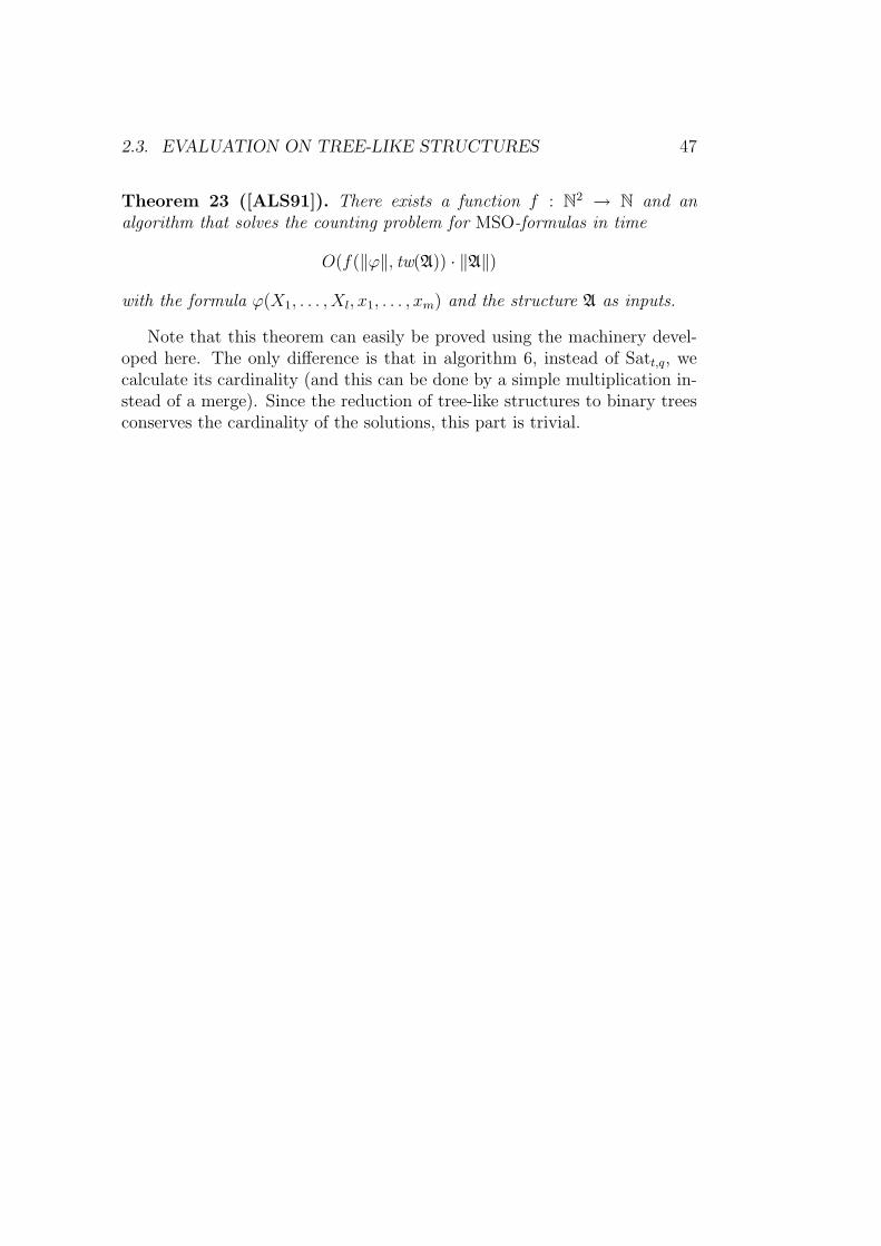
2.3. EVALUATION ON TREE-LIKE STRUCTURES 47
Theorem 23 ([ALS91]). There exists a function f : N2 → N and analgorithm that solves the counting problem for MSO-formulas in time
O(f(‖ϕ‖, tw(A)) · ‖A‖)
with the formula ϕ(X1, . . . , Xl, x1, . . . , xm) and the structure A as inputs.
Note that this theorem can easily be proved using the machinery devel-oped here. The only difference is that in algorithm 6, instead of Satt,q, wecalculate its cardinality (and this can be done by a simple multiplication in-stead of a merge). Since the reduction of tree-like structures to binary treesconserves the cardinality of the solutions, this part is trivial.

Chapter 3
First-order Properties overTree-decomposable Structures
In this chapter we present an extension of the notion of bounded tree-widthmotivated by the observation that common structures have the property thatthe tree-width only depends on the diameter of the structure. To capturethis behaviour, Eppstein [Epp99] introduced the diameter-treewidth propertyof graph classes.
Another way to look at this is that for these structures the tree-width ofa neighborhood of radius r ≥ 1 of an arbitrary vertex is bounded by f(r)for some suitable function f : N → N. We say that classes of structuressatisfying this property have bounded local tree-width. It turns out that oversuch classes the model checking problem is fixed parameter tractable. Inparticular, for each k ≥ 1 there is an f : N → N and an algorithm thatdecides A |= ϕ in time f(‖ϕ‖) · |A|1+1/k for ϕ ∈ FO.
Later on, we further restrict this notion to obtain a linear time algorithmfor the decision problem of FO on so called locally tree-decomposable classes.At the end of the chapter we examine the complexity of special versions ofthe presented algorithm and exhibit the crucial bottlenecks.
3.1 Local tree-likeness
Let A be a τ -structure for some vocabulary τ . Recall that by G(A) we denoteits Gaifman graph. The distance dA(a, b) between two elements a, b ∈ Ain A is the length dA(a, b) of the shortest path in G(A) connecting a andb. For r ≥ 1 and a ∈ A we define the r-neighborhood of a in A to beNAr (a) := b ∈ A | dA(a, b) ≤ r.
48

3.1. LOCAL TREE-LIKENESS 49
Definition 24. (1) The local tree-width of a structure A is the functionltwA : N→ N defined by
ltwA(r) := max
tw(〈NAr (a)〉)
a ∈ A.(2) A class C of structures has bounded local tree-width, if there is a func-
tion f : N→ N such that ltwA(r) ≤ f(r) for all A ∈ C, r ∈ N.
There are several important classes of structures (graphs) that havebounded local tree-width.
Example 25. Structures of bounded tree-width. Let A be a structure withtw(A) ≤ w. Then ltwA(r) ≤ w for all r ≥ 1.
The degree of an element a ∈ A of a structure A is the size of its 1-neighborhood, |NA
1 (a)|. The degree of a structure A is the maximal degreerealized by an element of A.
Example 26. Structures of bounded degree. Let A be a structure of degreeat most d, for a d ≥ 1. Then ltwA(r) ≤ d(d− 1)r−1 for all r ≥ 1.
With reference to the Gaifman graph we can extend the notion of pla-narity to arbitrary structures. We say that a structure A is planar if thecorresponding Gaifman graph G(A) is planar. Observe that a structure al-ways has the same local tree-width as its Gaifman graph. Hence, all boundson graph classes presented in the sequel extend to the corresponding classesof structures.
Example 27 (Robertson and Seymour [RS84]). Planar graphs. Theclass of planar graphs has bounded local tree-width. More precisely, forevery planar graph G and r ≥ 1 we have ltwG(r) ≤ 3r.
Example 28 (Eppstein [Epp99]). Graphs of bounded genus. Let S be asurface. Then the class of all graphs embeddable in S has bounded localtree-width. More precisely, there is a constant c ≥ 1 such that for all graphsG embeddable in S and for all r ≥ 1 we have ltwG(r) ≤ c · g(S) · r (here g(S)denotes the genus of the surface S).
A minor of a graph G is a graph H that is obtained from a subgraphof G by contracting edges. Classes of embeddable graphs (these includeplanar graphs) are examples of minor-closed graph classes. Eppstein gavethe following characterization of all classes of bounded local tree-width thatare closed under taking minors. An apex graph is a graph G that has a vertexv ∈ G such that G \ v is planar.

50 CHAPTER 3. FIRST-ORDER DECISION PROBLEMS
Theorem 29 (Eppstein [Epp95, Epp99]). Let C be a minor-closed classof graphs. Then C has bounded local tree-width if, and only if, C does notcontain all apex graphs.
Let Km,n be the complete bipartite graph with parts of size n and m,respectively.
Example 30. K3,m free graphs. Let C be a class of graphs that do notcontain all K3,m as minors. Then C has bounded local tree-width.
This follows immediately from the observation that K3,m, for m ≥ 3, isan apex graph.
Observe that the class of structures of bounded degree is the only examplethat is not closed under taking minors.
Neighborhood and tree covers: A successful way to examine local prop-erties of structures is to cover them by small neighborhoods. This has beendone systematically in, for instance, [ABCP93, AP90, Pel93].
Definition 31. Let r, s ≥ 1. An (r, s)-neighborhood cover of a structure A
is a family N of subsets of A with the following properties:
(1) For every a ∈ A there exists an N ∈ N such that NAr (a) ⊆ N .
(2) For every N ∈ N there exists an a ∈ A such that N ⊆ NAs (a).
For a subset N of the universe of a structure A, the set of vertices a ∈ Nsuch that NA
r (a) ⊆ N is denoted by Kr(N). Covers are coded as lists of lists(recall the definition of big objects in section A.3). Hence the size of a familyN of sets is ‖N‖ :=
∑N∈N |N |. The algorithm in the following lemma is an
adaptation of an algorithm due to Peleg [Pel93] to our situation.
Lemma 32 (Peleg [Pel93]). Let k ≥ 1. Then there is an algorithm that,given a graph G and an r ≥ 1, computes an (r, 2kr)-neighborhood cover Nof G of size ‖N‖ = O(|G|1+1/k) in time O(
∑N∈N ‖〈N〉G‖).
Proof: We compute the cover as it is displayed in algorithm 12. We iter-atively compute a neighborhood cover N , maintaining a set H of verticeswhose r-neighborhood has not yet been covered by a set in N . In each it-eration step of the main loop (lines 4-14), the algorithm picks an arbitraryvertex a from H (actually the first in the list) and starts to compute increas-ing neighborhoods of a (in lines 7-11) until a certain threshold is reached(line 11). Then it adds the computed set N to the cover N and removes

3.1. LOCAL TREE-LIKENESS 51
1 proc comp cover(G, r)2 H := copy(G); n := |G|3 N := ∅;4 while H 6= ∅ do5 a := first(H);6 N := a;7 do8 M := copy(N);9 L := NGr (M) ∩H;
10 N := NGr (L);11 od while |N | > n1/k|M |12 N := N ∪ N;13 H := H \ L;14 od15 .
Algorithm 12. Computing a neighborhood-cover of G
all points whose neighborhood has now been covered from H, before it goesto the next iteration of the main loop. This process is repeated until H isempty.
Correctness: Let G be a graph, r ≥ 1 and N the cover computed by thealgorithm. We prove a series of claims which entail the statement of thelemma.
Claim 1: For every a ∈ G there exists an N ∈ N such that Nr(a) ⊆ N .
Proof: An element a is removed from the set H of uncovered elements ofA in line 13 only if it belongs to a set L such that N := NGr (L) has beenadded to N . Hence this N contains NGr (a). This proves Claim 1.
Claim 2: For every N ∈ N there exists an a ∈ G such that N ⊆ NG2kr(a).
Proof: We consider the iteration of the main loop that leads to N . Let abe the element chosen in line 5, and let N0 := a. Let l ≥ 1 be the numberof times the loop in lines 7-11 is repeated. For 1 ≤ i ≤ l, let Ni be the valueof N after the ith iteration. Then for 1 ≤ i ≤ l−1 we have |Ni| > n1/k|Ni−1|,and therefore |Ni| > ni/k. Thus l ≤ k.
Furthermore, it is easy to see that for 1 ≤ i ≤ l we have Ni ⊆ NG2ir(a).This implies Claim 2.

52 CHAPTER 3. FIRST-ORDER DECISION PROBLEMS
Claims 1 and 2 show that N is indeed an (r, 2kr)-neighborhood cover ofG. The following Claim 3 shows that the cover is not too large.
Claim 3. ‖N‖ ≤ n1+(1/k).
Proof: For N ∈ N , let M be the corresponding set that is computed inthe last iteration of the loop in lines 7-11 that let to N (i.e. M is the valueof N after the second but last iteration of the loop).
We first show that for distinct N1, N2 ∈ N we have M1 ∩M2 = ∅. Tosee this, suppose that N1 is computed first. Let H1 be the value of H afterthe iteration of the main loop in which N1 has been computed. Note thatfor every a ∈ M1 and b ∈ H1 we have dG(a, b) > r. Moreover, M2 ⊆ N2 ⊆NGr (H1). Thus M1 ∩M2 = ∅.
By the condition in line 11, we have |N | ≤ n1/k|M | for all N ∈ N , henceobtain
‖N‖ =∑N∈N
|N | ≤ n1/k∑N∈N
|M | ≤ n1/k · n.
The last inequality holds because the M are disjoint subsets of G. Thisproves Claim 3.
Running time: To estimate the running time of the algorithm, we claimthat each iteration of the main loop requires time O(‖〈N〉‖), for the vertexset N added to N in the corresponding iteration pass. Then the entirealgorithm runs in the claimed time bound.
All sets except for H are implemented as lists. For H we must be able tocompute set differences H \L for some list L (line 13) and to check whetherH 6= ∅ (and if so, provide an example). We fit these requirements by using areferenced list as described in appendix A on page 108.
We prove the claimed time bound for each single iteration. To calculateL in line 9 we perform a multi-source breadth-first search starting in M . Toassure that we stay within H, we additionally check for new vertices, if theybelong to H (this takes constant time). Observe that we possibly consideredges that are not contained in 〈L〉G, but these are all contained in N , whichis built in the subsequent line. Furthermore, each of these edges is consideredat most r many times (the depth of the search tree). Thus, together we needat most O(‖〈N〉‖) steps.
Note the impact of the usage of referenced lists on the running time:we remove a set L (given as a list) from H calling the subroutine remove()displayed as algorithm 29 (in the appendix). Removing m vertices takes timeO(m). The emptiness check in line 4 and providing an example a ∈ H inline 5 needs constant time.
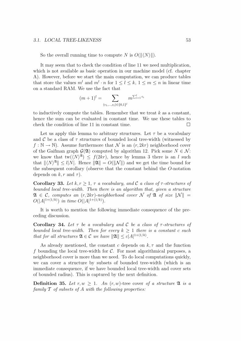
3.1. LOCAL TREE-LIKENESS 53
So the overall running time to compute N is O(‖〈N〉‖).
It may seem that to check the condition of line 11 we need multiplication,which is not available as basic operation in our machine model (cf. chapterA). However, before we start the main computation, we can produce tablesthat store the values ml and ml · n for 1 ≤ l ≤ k, 1 ≤ m ≤ n in linear timeon a standard RAM. We use the fact that
(m+ 1)l =∑
(ε1,...,εl)∈0,1lm∑li=1 εi
to inductively compute the tables. Remember that we treat k as a constant,hence the sum can be evaluated in constant time. We use these tables tocheck the condition of line 11 in constant time. 2
Let us apply this lemma to arbitrary structures. Let τ be a vocabularyand C be a class of τ structures of bounded local tree-width (witnessed byf : N → N). Assume furthermore that N is an (r, 2kr) neighborhood coverof the Gaifman graph G(A) computed by algorithm 12. Pick some N ∈ N :we know that tw(〈N〉A) ≤ f(2kr), hence by lemma 3 there is an l suchthat ‖〈N〉A‖ ≤ l|N |. Hence ‖A‖ = O(‖N‖) and we get the time bound forthe subsequent corollary (observe that the constant behind the O-notationdepends on k, r and τ).
Corollary 33. Let k, r ≥ 1, τ a vocabulary, and C a class of τ -structures ofbounded local tree-width. Then there is an algorithm that, given a structureA ∈ C, computes an (r, 2kr)-neighborhood cover N of A of size ‖N‖ =O(|A|1+(1/k)) in time O(|A|1+(1/k)).
It is worth to mention the following immediate consequence of the pre-ceding discussion.
Corollary 34. Let τ be a vocabulary and C be a class of τ -structures ofbounded local tree-width. Then for every k ≥ 1 there is a constant c suchthat for all structures A ∈ C we have ‖A‖ ≤ c|A|1+(1/k).
As already mentioned, the constant c depends on k, τ and the functionf bounding the local tree-width for C. For most algorithmical purposes, aneighborhood cover is more than we need. To do local computations quickly,we can cover a structure by subsets of bounded tree-width (which is animmediate consequence, if we have bounded local tree-width and cover setsof bounded radius). This is captured by the next definition.
Definition 35. Let r, w ≥ 1. An (r, w)-tree cover of a structure A is afamily T of subsets of A with the following properties:

54 CHAPTER 3. FIRST-ORDER DECISION PROBLEMS
(1) For every a ∈ A there exists a T ∈ T such that NAr (a) ⊆ T .
(2) For every T ∈ T we have tw(〈T 〉A) ≤ w.
The next lemma concerns computing the substructures induced by thesets of a tree cover. This computation is necessary for most algorithms thatwork on the cover sets.
Lemma 36. Let T be an (r + 1, w)-tree cover for a structure A, r, w ≥1. Then an (r, w)-tree cover T ′ and the set 〈T ′〉A | T ′ ∈ T ′ of inducedstructures can be computed in time
O(∑T∈T
‖〈T 〉A‖).
Proof: Let T be an (r+ 1, w)-tree cover of a structure A for some r, w ≥ 1.Take an arbitrary T ∈ T . We call a vertex v ∈ T outermost, if there is anadjacent vertex u ∈ A \ T . In a first step, we copy all but the outermostvertices in T , to a separate list T ′. This is done by a breadth-first search,which terminates a branch, when a vertex outside T is to be put into thequeue (cf. the standard implementation of a breadth-first search tree usingqueues). Then for each v ∈ T ′ we copy its adjacency list, leaving out theedges to vertices not in T ′. Obviously, we obtain 〈T ′〉 and furthermore allthe T ′ form an (r, w)-neighborhood cover of A.
Concerning the running time, observe that the set T ′ can be found intime O(‖〈T ′〉‖) (since for the outermost vertices we only consider one edgeper vertex that is not contained in E〈T 〉). The same time bound holds forthe second step. 2
The construction of tree covers defined in the next lemma is implicit in[Epp99].
Lemma 37 (Eppstein [Epp99]). Let r ≥ 1 and C be a class of graphsthat is closed under taking minors and has bounded local tree-width. Letf : N→ N be a function bounding the local tree-width of the graphs in C.
Then there is an algorithm that, given a graph G ∈ C, computes an(r, f(2r + 1))-tree cover T of G of size ‖T ‖ = O(|G|) in time O(|G|).
Proof: Let G ∈ C and choose an arbitrary vertex a0 ∈ G. For 0 ≤ i ≤ j, letG[i, j] := a ∈ G | i ≤ dG(a0, a) ≤ j.
We claim that tw(〈G[i, j]〉) ≤ f(j − i + 1). This is immediate if i = 0or i = 1, because then G[i, j] ⊆ NGj (a0). If i > 1, we simply contract theconnected subgraph 〈G[0, i − 1]〉G to a single vertex b0. We obtain a minor

3.1. LOCAL TREE-LIKENESS 55
G ′ of G, which is also an element of C by our assumption that C is closedunder taking minors. G ′ still contains the set G[i, j] as it is, but now this setis contained in NG
′
j−i+1(b0). This proves the claim.
The claim implies that for all r ≥ 1, the family T := G[i, i+ 2r] | i ≥ 0is an (r, f(2r+1))-tree cover of G of size at most (2r+1)|G|. On input G, wecan choose an arbitrary a0 and then compute this tree cover in linear timeby a breadth-first search. 2
It is not clear at all, whether we can find an (r, s)-neighborhood coverN for planar graphs G in O(|G|) steps, for fixed r, s ≥ 1, while the aboveconstruction offers an easy and effective way to compute tree covers. Treecovers of size linear in the size of the structure and a linear time algorithmcomputing such a cover is exactly what we need in our algorithms. Thefollowing definition makes this precise.
Definition 38. A class C of structures is locally tree-decomposable, if thereis an algorithm that, given an r ≥ 1 and a structure A ∈ C, computes an(r, w)-tree cover T of A (for some suitable w ≥ 1 depending only on r) suchthat ‖T ‖ = O(|A|) in time O(|A|).
Immediately, we get a lemma corresponding to lemma 3 saying that lo-cally tree-decomposable classes are sparse.
Corollary 39. Let τ be a vocabulary and C be a locally tree-decomposableclass of τ -structures. Then there is a c ≥ 1 such that for all structures A ∈ Cwe have ‖A‖ = c · |A|.
Observe that the constant c depends on τ and the value w bounding thetree-width of the parts of the cover.
Example 40. Classes closed under taking minors. Classes of planar graphs,of graphs of bounded genus, andK3,m-free classes that are closed under takingminors are locally tree-decomposable.
This follows immediately from lemma 37 and the fact that all these classeshave bounded local tree-width. Although not closed under minors, classesof graphs of bounded degree are locally tree-decomposable. Let C be a classof graphs with degree bounded by, say, d and r ≥ 1. Then the familyNGr (v) | v ∈ G is an (r, d(d− 1)r−1)-tree cover of G of size |G| · d(d− 1)r−1.
Example 41. Graphs of bounded degree. The class of graphs of boundeddegree is locally tree-decomposable.

56 CHAPTER 3. FIRST-ORDER DECISION PROBLEMS
Remark: If we carefully analyse the covers constructed in all examples,we find that either a cover consists of subsets with constant radius, or ofrings of constant breadth. For the rings, to deduce bounded tree-width, wecontract their interior to a single vertex and apply the bounded local tree-width property. For subsets with constant radius, the only example is theclass of graphs of bounded degree. This appears to be a “natural” dichotomy,since only artificial classes of locally bounded tree-width, not closed underminors, with unbounded valence are known (e.g. bounded degree plus alltrees). Recently Eppstein [Epp99] asked, if at all there is any other “natural”family of graphs, not minor-closed, but with bounded local tree-width.
Naturally the question arises, if classes of bounded local tree-width aresparse (recall that corollary 34 gave an upper bound of the size of suchstructures). The following counter example was provided by Grohe [FG99]and shows that local tree-decomposability is a proper restriction of boundedlocal tree-width.
Example 42. We construct a class C of graphs of bounded local tree-widthsuch that for every constant c there is a graph G ∈ C with ‖G‖ ≥ c|G|.
We use the following theorem due to Erdos [Erd59]: For all g, k ≥ 1 thereexists a graph of girth greater than g and chromatic number greater than k.Remember that the girth g(G) of a graph G is the length of the shortest cyclein G and the chromatic number χ(G) of G is the least number of colors neededto color the vertices of G such that no two adjacent vertices have the samecolor. It is easy to see that every graph G with χ(G) ≥ k has a connectedsubgraph H with average degree
2|EH||H|
≥ k − 1
(cf. [Die97], p. 98). The diameter of a connected graph G is the numberdiam(G) := maxdG(a, b) | a, b ∈ G.
We inductively construct a family (Gi)i≥1 of graphs as follows: G1 is thegraph consisting of two vertices and an edge between them. Suppose nowthat Gi is already defined. Let G ′i+1 be a graph with g(G ′i+1) ≥ 2diam(Gi) + 1and χ(G ′i+1) ≥ 2i+ 3. Let Gi+1 be a connected subgraph of G ′i+1 with
2|EGi+1||Gi+1|
≥ 2i+ 2.
Clearly, g(Gi+1) ≥ g(G ′i+1) ≥ 2diam(Gi) + 1.Observe that for every r ≥ 1 and every graph G, if 2r + 1 < g(G) then
ltwG(r) ≤ 1. Moreover, if G is connected then ltwG(r) = tw(G) for all

3.2. GAIFMAN’S THEOREM 57
r ≥ diam(G). For every i ≥ 1 and diam(Gi) ≤ r < diam(Gi+1), we letf(r) := maxtw(Gi), ltwGi+1(r). We claim that ltwGi(r) ≤ f(r) for all i, r ≥1. This is obvious for i = 1. For i ≥ 2, we have to distinguish betweenthree cases: If r < diam(Gi−1) ≤ 1
2(g(Gi) − 1), then ltwGi(r) ≤ 1 ≤ f(r).
If diam(Gi−1) ≤ r < diam(Gi), then ltwGi(r) ≤ f(r) immediately by thedefinition of f . If r ≥ diam(Gi), then ltwGi(r) = tw(Gi) ≤ f(r).
Thus the class C := Gi | i ≥ 1 has bounded local tree-width. On theother hand, for every i ≥ 2 we have ‖Gi‖ ≥ |EGi| ≥ i|Gi|.
3.2 Gaifman’s theorem
Recall the definition of the distance between two elements of a relationalstructure. Let τ be a vocabulary. Then for every r ≥ 1 there is a formulaδr(x, y) ∈ FO[τ ] such that for all τ -structures A and a, b ∈ A we have A |=δr(a, b) ⇔ dA(a, b) ≤ r. Within formulas we write d(x, y) ≤ r instead ofδr(x, y) and d(x, y) > r instead of ¬δr(x, y).
If ϕ(x) is a first-order formula, then ϕNr(x)(x) is the formula obtainedfrom ϕ(x) by relativizing all quantifiers to Nr(x), that is, by replacing everysubformula of the form ∃yψ(x, y, z) by ∃y(d(x, y) ≤ r ∧ψ(x, y, z)) and everysubformula of the form ∀yψ(x, y, z) by ∀y(d(x, y) ≤ r → ψ(x, y, z)). Aformula ψ(x) of the form ϕNr(x)(x), for some ϕ(x), is called r-local . Thebasic property of r-local formulas ψ(x) is that it only depends on the r-neighborhood of x whether they hold at x or not, that is, for all structuresA and a ∈ A we have A |= ψ(a) ⇐⇒
⟨NAr (a)
⟩|= ψ(a).
The next theorem is due to Gaifman and states that properties expressiblein first-order logic are local.
Theorem 43 (Gaifman [Gai82]). Every first-order sentence is equivalentto a Boolean combination χ of sentences of the form
∃x1 . . . ∃xm( ∧
1≤i<j≤m
d(xi, xj) > 2r ∧∧
1≤i≤m
ψ(xi)), (3.1)
for suitable r,m ≥ 1 and an r-local ψ(x). The minimal r satisfying the aboveproperties is called the locality rank of ϕ.
In other words, for every sentence ϕ ∈ FO there is a Boolean formula Fand sentences χ1, . . . , χl of the form (3.1) such that F (χ1, . . . , χl) is equivalentto ϕ.
Recall that rk(ϕ) denotes the maximal number of quantifier nestings inϕ. The original proof of Gaifman yielded r ≤ 7rk(ϕ)−1 and m ≤ rk(ϕ).

58 CHAPTER 3. FIRST-ORDER DECISION PROBLEMS
Gaifman presented an explicit inductive construction of the formula χ. Thisenables the effective computation of this formula by an algorithm in time,say, f(‖ϕ‖), for some suitable f : N → N (this function is assumed to benon-elementary [Woe00a]).
3.3 The main algorithm
In this final section we will present the main result of this chapter, namely, analgorithm that decides A |= ϕ for structures A of bounded local tree-widthand first-order sentences ϕ.
Roughly, we first compute the formula χ (from Gaifman’s theorem) thatw.l.o.g. has the form (3.1). Then, using a tree cover T of A, we mark thoseelements a ∈ A for which we have A |= ψ(a). In a last step we try to findelements a1, . . . , am ∈ A such that dA(ai, aj) > 2r for all i 6= j. If there aresuch elements, we accept and reject, otherwise.
We start with two lemmas comprising the main difficulties of the algo-rithm. Assume that we have a family T of subsets of A. The first lemmais needed to recognize those elements a of a T ∈ T for which A |= ψ(a) isequivalent to 〈T 〉A |= ψ(a) (ψ(x) is assumed to be r-local), i.e. the sets ofelements a ∈ T such that NA
r (a) ⊆ T .
Lemma 44. Let A be a τ -structure and T a family of subsets of A. Thenthere exists an algorithm that computes the sets Kr(T ) for all T ∈ T in time
O(∑t∈T
‖〈T 〉A‖).
Proof: Recall that Kr(T ) := a ∈ T | NAr (a) ⊆ T. Let G := G(A) be the
Gaifman graph of A. We present an algorithm that computes Kr(T ) in timeO(‖〈T 〉A‖) for each T ∈ T .
Sets T of a cover are given as a list a1, . . . , al. The pseudo-code forour algorithm is displayed as algorithm 13. We compute Kr(T ) iteratively,maintaining a set K that, in the ith pass, contains the set a ∈ T | NA
i (a) ⊆T. We code K by a referenced list (see page 108) what allows containmentchecks a ∈ K and removing elements in constant time. For simplicity, wedenote the entire data structure by kernel and remove elements by a call ofremove.
Observe that, in contrast to the last usage of a referenced list, we do notrequire to read out single elements from K. Hence, it would suffice to codeK by the two arrays refc, contr (cf. the definition of referenced lists).

3.3. THE MAIN ALGORITHM 59
1 proc comp kernel(T, r)2 kernel := copy(T ); /* working copy of T */3 ref init(kernel); /* initialize referenced array */4 for i = 1 to r do5 aux := ∅;6 for a ∈ kernel do7 if a has a neighbor b /∈ kernel8 then9 append(aux, a);
10 fi11 od12 for b ∈ aux do remove(kernel, b) od13 od14 return(kernel);15 .
Algorithm 13. Compute Kr(T ) for some T .
It is quite obvious that function comp kernel works correctly. Observethat the condition in line 7 characterizes the elements of kernel that lie onthe outermost ring. To check this condition we have to go through the list ofvertices adjacent to a, hence this requires constant time for each such edge(the append in the subsequent line also takes constant time).
Running time: So let us analyse the running time of the algorithm. Eachpass of the outer loop over i needs time O(|T |): in particular we need O(|EA∩T 2|) steps for line 7 plus O(|T |) for line 12. Together this is O(|T | + |EA ∩T 2|) = O(‖〈T 〉‖) = O(|T |).
Since r is treated as a constant, the overall time need for the subroutineis O(|T |) as claimed above. 2
The next lemma allow to determine, whether there is a certain numberof elements whose pairwise distance is bigger than a given r.
Lemma 45. Let C be a class of τ -structures of bounded local tree-width andr,m ≥ 1. Then there is an algorithm that, given a structure A ∈ C and a setP ⊆ A, decides if there are a1, . . . , am ∈ P such that
dA(ai, aj) > r for 1 ≤ i < j ≤ m. (*)
Furthermore, this algorithm needs time O(|A|).

60 CHAPTER 3. FIRST-ORDER DECISION PROBLEMS
1 proc find remotes(A, P,m, r)2 valid := copy(P ); p := 0;3 ref init(valid);4 while valid 6= ∅ and p < m do5 p := p+ 1; ap := first(valid);6 valid := valid \NA
r (ap);7 od8 if p = m then9 accept
10 else if l = 0 then reject fi11 fi12 H := (NA
2r(a1, . . . , ap), P );13 if there are pairwise remote a1, . . . , am ∈ H14 then15 accept;16 else17 reject;18 fi19 .
Algorithm 14. Decide if the are m remote vertices in P .
Proof: Let f : N → N be a function that guarantees that C is of boundedlocal tree-width. The decision procedure is displayed as algorithm 14
Correctness: The algorithm essentially involves two phases. In the firstphase (lines 2-7) we compute elements a1, . . . , ap such that dA(ai, aj) > r forsome p ≤ m. If p = m then we are done and the algorithm accepts, if p = 0(this means P = ∅) we reject. Otherwise (p < m), we pass over to the secondphase.
When we enter the second phase, we have P ⊆ NAr (a1, . . . , ap), since
otherwise we would find another ap+1 remote (with distance > r) to allpreceding ai. Let H := (〈NA
2r(a1, . . . , ap), P )〉. Then for all b, b′ ∈ P wehave dA(b, b′) ≤ r ⇐⇒ dH(b, b′) ≤ r (since we included the r-neighborhoodof P ). Thus, there are a1, . . . , am ∈ P satisfying (*) in A if and only if theysatisfy (*) in H. This proves the correctness of the algorithm.
Running time: The first phase requires O(|A|) steps, since the loop ispassed through at most m times and each pass requires at most O(|A|) steps(set minus is done using a referenced list). For the second phase, note that for

3.3. THE MAIN ALGORITHM 61
B of constant size and s ≥ 1 we have ‖〈NAs (B)〉‖ = O(|NA
s (B)|) (by boundedlocal tree-width). Thus H can be calulated in time O(‖〈H〉‖) = O(|H|).
Furthermore we have tw(H) ≤ ltwA(2pr) ≤ f(2pr), hence the conditionin line 13 is equivalent to the satisfaction of the first-order formula
∃x1, . . . , xm∧
1≤i<j≤m
d(xi, xj) > r ∧m∧i=1
Pxi
in H, and can thus be checked in time O(|H|) by Courcelle’s theorem (theo-rem 9). 2
Now we are ready to state and prove the main theorems.
Theorem 46. Let C be a class of structures of bounded local tree-width. Thenfor every k there is an algorithm that, on input A ∈ C and ϕ ∈ FO, decidesA |= ϕ in time
f(‖ϕ‖) · |A|1+(1/k)
for some suitable function f : N→ N.
Proof: Algorithm 15 is claimed to do the job.
Algorithm 15: Deciding A |= ϕ
Input: Structure A ∈ C, FO-sentence ϕOutput: A |= ϕ?
1. Compute F (χ1, . . . , χl) according to the recipe given by Gaifman’s the-orem; let r and m denote the values from Gaifman’s theorem
2. Compute an (r + 1, 2k(r + 1)) neighborhood-cover N ′ of A
3. Compute an (r, w)-tree cover N from N ′ (for some suitable w ≥ 1)plus the corresponding induced structures
4. Compute Kr(N) for all N ∈ N
5. for all i = 1, . . . , l: (ψi denotes the local formula in χi)
i. Compute PN := a ∈ N | NAr (a) ⊆ N, 〈N〉 |= ψi(a) for all
N ∈ Nii. Compute P :=
⋃N∈N PN
iii. if there are a1, . . . , am ∈ P such that dA(ai, aj) > 2r for i 6= j thenpi := true, else pi := false
6. if F (p1, . . . , pl) = true then accept, else reject

62 CHAPTER 3. FIRST-ORDER DECISION PROBLEMS
Correctness: Since C has bounded local tree-width, the (r + 1, 2k(r + 1))-neighborhood cover N computed in line 2 is a (r + 1, w)-tree cover for somesuitable w ≥ 1 (only depending on C and r). Hence, we can apply lemma 36to get a (r, w)-tree cover N with the corresponding induced substructures.The remainder is obviously correct.
Running time: By Gaifman’s theorem and the subsequent remark, the firstline needs O(f(‖ϕ‖)) steps. Line 2 requires time O(|A|1+(1/k)) (by lemma 32).Recall that the obtained neighborhood cover has size ‖N‖ = O(|A|1+(1/k)).By lemma 44, step 4 needs time O(‖N‖).
l is bounded by a function on ‖ϕ‖, hence we restrict attention to onecycle of the loop. Step 5i is performed by a call of the algorithm from lemma12 for all N ∈ N , each of which requires O(g(‖ϕ‖) · |N |) time. Together, thistakes O(‖ϕ‖·‖N‖) time. Line 5ii takes time O(|N |) and finally, using lemma45 we can decide if the sought elements exist in time O(|A|). Altogether, weget the desired time bound. 2
If we have a locally tree-decomposable class C, we can do even better.
Theorem 47. Let C be a locally tree-decomposable class of structures. Thenthere exists an algorithm that, on input A ∈ C and ϕ ∈ FO, decides A |= ϕin time
f(‖ϕ‖) · ‖A‖for some suitable function f : N→ N.
Proof: The algorithm works exactly like in the previous theorem with theonly difference that now, instead of computing a neighborhood-cover, wedirectly compute a tree cover T and the corresponding induced substructures.By the assumption on C being locally tree-decomposable this can be done intime O(|A|) (cf. the definition). Since T has size O(|A|) and the rest of thealgorithm works in time O(‖T ‖), we are done. 2
Remark: The constants involved in the running time depend on the classC, that is, on a function g such that for r ≥ 1,A ∈ C there is a (r, g(r))-treecover of A.
3.4 Remarks on special cases
The results of the previous section cover a big variety of different problems.Due to their meta character, there are important drawbacks on the efficiency

3.4. REMARKS ON SPECIAL CASES 63
of the algorithms. These are caused by their design, which followed theguideline of being as universal as possible.
For particular cases, these general algorithms can be adjusted to get bet-ter constants. We are going to discuss the restriction of both, the class ofadmitted structures as well as the admitted formulas.
Recall the algorithm from theorem 47. Essentially, given a structureA and an FO-sentence ϕ, the algorithm proceeds in four steps. First, wecompute the Gaifman normal form for ϕ, which is w.l.o.g. of the form
∃x1 . . . ∃xm( ∧
1≤i<j≤m
d(xi, xj) > 2r ∧∧
1≤i≤m
ψ(xi)),
where ψ(x) is an r-local formula for some suitable r ≥ 1 (the locality rank).Then, in the second step, a suitable cover for A (this part depends on theadmitted class; cf. the definition of locally tree-decomposable) is computed.
Using theorem 21, we compute the set P := a ∈ A | A |= ψ(a) in thethird step, and finally, we try to find a constant number of pairwise “remote”elements from P . A closer look shows that each step bears its problems withrespect to the running time.
(i) For the computation of the Gaifman normal form, there is no exactbound known, but already easy formulas tend to yield big and complicatedlocal formulas. For more details the reader is referred to the original workof Gaifman in which an inductive construction of the sought formula is pre-sented.
(ii) Well known is the problem of computing a tree decomposition for astructure. As already discussed in the preceding chapter (cf. page 18) nopractical algorithm is known for the general case.
(iii) Essentially the same holds for the Courcelle-like evaluation algorithmemployed to compute P . But although the worst case analysis yields a lowerbound consisting of a tower of height q, if q is the number of quantifieralternations of ψ, it turned out that for most cases the algorithm behaveswell. Hence, apart from the problem of getting a tree-decomposition, thispart can be considered as practical (or at least more practical than the otherparts).
(iv) Since for the last step we again need Courcelle’s method, there arethe same objections against practicability as in (ii) and (iii).

64 CHAPTER 3. FIRST-ORDER DECISION PROBLEMS
In the remainder of this section, we exemplarily show how different restric-tions affect the algorithms and their running time. In particular, we considerthe restricitions to structures of bounded degree, planar structures and exis-tential formulas.
Structures of bounded degree: For this case, the Gaifman part remainsthe same since we treat arbitrary first-order formula ϕ. Assume that A
denotes the input structure. In part (ii) and (iii), we first compute the setsNAr (a) for all v ∈ A and suitable r ≥ 1, and then apply Courcelle’s algorithm
to determine whether or not ψ(a) holds in A. The application of Courcelle’stheorem is possible due to the fact that each NA
r (a) has size at most f(r) forsome function f , hence has tree-width only depending on r. An alternativeto Courcelle’s algorithm on tree-width f(r) is the ad-hoc algorithm for first-order logic with l variables (see theorem 1) requiring time O(f(r)l) withvery low constants hidden behind the O-notation (cf. the description of thealgorithm on page 13).
Note that this does not necessarily provide a better running time. But itlooks more feasible than the general approach. The same can be said aboutthe last step of the algorithm, where we tried to find pairwise remote vertices.Here we similarly adapt the general algorithm to the special case and decideline 13 in algorithm 14 by an exhaustive search in the substructure H (sincethe size of H only depends on r). Another possiblity would be to adjustDijkstra’s algorithm to our setting.
The same ideas led Grohe [Gro00] to the definition of structure classesof low degree. We say that a class of structures C is of low degree, if forevery k ≥ 1 there is an nk ≥ 1 such that for all A ∈ C with |A| ≥ nkwe have deg(A) ≤ |A|1/k. It is easy to see that the above modification ofthe algorithm also works for this class (observe that tree decompositions donot occur any more in the description of the algorithm). Given a k ≥ 1,the complexity analysis yields the upper time bound f(‖ϕ‖, k) · |A|1+1/k todecide A |= ϕ for some suitable function f .
Planar graphs: For planar graphs there are essentially two places wherewe can (apparently) speed-up the general algorithm. The first place is wherewe compute the tree-decomposition of a planar graph of bounded diameter.In [Epp95] an algorithm was described that computes a tree-decompositionof width O(diam(G)) of a planar graph G in time O(|G|). This algorithmessentially consists of a depth-first search through G and is thus quite effi-cient (in contrast to the algorithm from [Bod96] the constants hidden behindthe O-notation are low). Unfortunately, this algorithm does not provide a
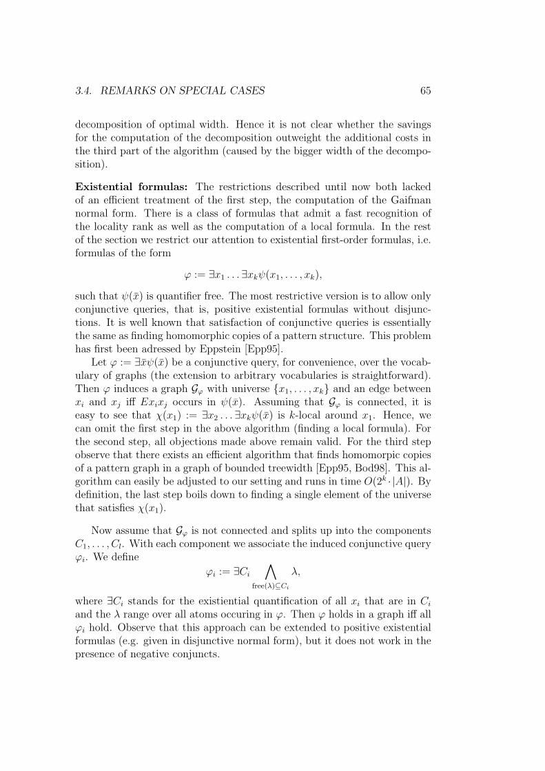
3.4. REMARKS ON SPECIAL CASES 65
decomposition of optimal width. Hence it is not clear whether the savingsfor the computation of the decomposition outweight the additional costs inthe third part of the algorithm (caused by the bigger width of the decompo-sition).
Existential formulas: The restrictions described until now both lackedof an efficient treatment of the first step, the computation of the Gaifmannormal form. There is a class of formulas that admit a fast recognition ofthe locality rank as well as the computation of a local formula. In the restof the section we restrict our attention to existential first-order formulas, i.e.formulas of the form
ϕ := ∃x1 . . . ∃xkψ(x1, . . . , xk),
such that ψ(x) is quantifier free. The most restrictive version is to allow onlyconjunctive queries, that is, positive existential formulas without disjunc-tions. It is well known that satisfaction of conjunctive queries is essentiallythe same as finding homomorphic copies of a pattern structure. This problemhas first been adressed by Eppstein [Epp95].
Let ϕ := ∃xψ(x) be a conjunctive query, for convenience, over the vocab-ulary of graphs (the extension to arbitrary vocabularies is straightforward).Then ϕ induces a graph Gϕ with universe x1, . . . , xk and an edge betweenxi and xj iff Exixj occurs in ψ(x). Assuming that Gϕ is connected, it iseasy to see that χ(x1) := ∃x2 . . . ∃xkψ(x) is k-local around x1. Hence, wecan omit the first step in the above algorithm (finding a local formula). Forthe second step, all objections made above remain valid. For the third stepobserve that there exists an efficient algorithm that finds homomorpic copiesof a pattern graph in a graph of bounded treewidth [Epp95, Bod98]. This al-gorithm can easily be adjusted to our setting and runs in time O(2k · |A|). Bydefinition, the last step boils down to finding a single element of the universethat satisfies χ(x1).
Now assume that Gϕ is not connected and splits up into the componentsC1, . . . , Cl. With each component we associate the induced conjunctive queryϕi. We define
ϕi := ∃Ci∧
free(λ)⊆Ci
λ,
where ∃Ci stands for the existiential quantification of all xi that are in Ciand the λ range over all atoms occuring in ϕ. Then ϕ holds in a graph iff allϕi hold. Observe that this approach can be extended to positive existentialformulas (e.g. given in disjunctive normal form), but it does not work in thepresence of negative conjuncts.

66 CHAPTER 3. FIRST-ORDER DECISION PROBLEMS
In his Master Thesis [Woe00b], Wohrle exhibited a bigger fragment ofexistential first-order logic that admits an easy treatment with respect tolocal behaviour. Recall the definition of Gϕ for a positive existential formulaϕ. For existential formulas ϕ, we define Gϕ to be equal to Gϕ′ , where ϕ′
results from ϕ by deleting all negative literals. Then ϕ is called guarded, iffor each ¬Exixj occuring in ϕ, the variables xi, xj are both contained in thesame component of Gϕ. In the thesis he was able to show that the algorithmfor positive existential formulas also works for guarded ones.
Conclusion: Are these specialized algorithms really practical? The com-putation of the Gaifman normal form in the first step not only takes a longtime, but also returns a huge formula, which afterwards has to be translatedto a finite automaton (including a further blow up). So the only practicalway seems to combine the above proposals, e.g. checking guarded existentialformulas over planar structures or structures of bounded degree.

Chapter 4
First-order Formulas with freeVariables
In the last section we haved showed that we can decide first-order proper-ties over locally tree-decomposable structures in linear time. Naturally, thequestion turns up, if the techniques applied successfully to the decision prob-lem, can be extended to get good algorithms for the evaluation and countingproblems.
Recall the problem: We are given a first-order formula ϕ(x) with freevariables x and a structure A. Our task is to design efficient algorithmsthat solve the evaluation, witness and counting problem, respectively, i.e.calculate the set ϕ(A), find a tuple a ∈ A such that A |= ϕ(a), or calculatethe number |ϕ(A)|.
We will proceed in three steps. In the first step, we develop a normal formfor local formulas ϕ(x). This normal form partitions the set ϕ(a) with respectto “distance-patterns” realized by the free variables x. Second, we include aspecial form of a tree cover T for A to get an alternative description of ϕ(A).This characterization describes how local solutions (computed in the coversets) are assembled to obtain the entire solution, which is accomplished by acombination of the locality properties of first-order logic and the respectiveproperties of neighborhood covers. These ingredients will yield an alternativecharacterization of ϕ(A), which will be the starting point for the solution ofthe three mentioned problems.
The particular solutions will be provided in a third step. While the eval-uation and witness case can be solved more or less straightforwardly, thecounting case requires a bit more effort.
67
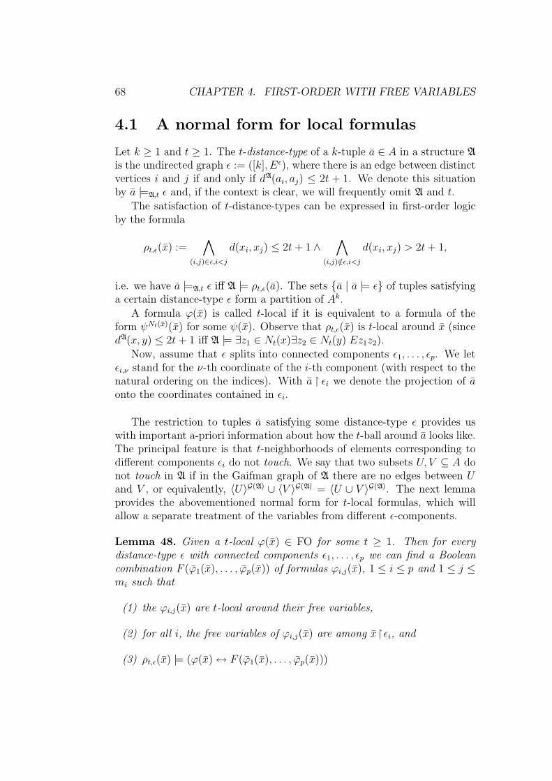
68 CHAPTER 4. FIRST-ORDER WITH FREE VARIABLES
4.1 A normal form for local formulas
Let k ≥ 1 and t ≥ 1. The t-distance-type of a k-tuple a ∈ A in a structure A
is the undirected graph ε := ([k], Eε), where there is an edge between distinctvertices i and j if and only if dA(ai, aj) ≤ 2t + 1. We denote this situationby a |=A,t ε and, if the context is clear, we will frequently omit A and t.
The satisfaction of t-distance-types can be expressed in first-order logicby the formula
ρt,ε(x) :=∧
(i,j)∈ε,i<j
d(xi, xj) ≤ 2t+ 1 ∧∧
(i,j)/∈ε,i<j
d(xi, xj) > 2t+ 1,
i.e. we have a |=A,t ε iff A |= ρt,ε(a). The sets a | a |= ε of tuples satisfyinga certain distance-type ε form a partition of Ak.
A formula ϕ(x) is called t-local if it is equivalent to a formula of theform ψNt(x)(x) for some ψ(x). Observe that ρt,ε(x) is t-local around x (sincedA(x, y) ≤ 2t+ 1 iff A |= ∃z1 ∈ Nt(x)∃z2 ∈ Nt(y) Ez1z2).
Now, assume that ε splits into connected components ε1, . . . , εp. We letεi,ν stand for the ν-th coordinate of the i-th component (with respect to thenatural ordering on the indices). With a εi we denote the projection of aonto the coordinates contained in εi.
The restriction to tuples a satisfying some distance-type ε provides uswith important a-priori information about how the t-ball around a looks like.The principal feature is that t-neighborhoods of elements corresponding todifferent components εi do not touch. We say that two subsets U, V ⊆ A donot touch in A if in the Gaifman graph of A there are no edges between Uand V , or equivalently, 〈U〉G(A) ∪ 〈V 〉G(A) = 〈U ∪ V 〉G(A). The next lemmaprovides the abovementioned normal form for t-local formulas, which willallow a separate treatment of the variables from different ε-components.
Lemma 48. Given a t-local ϕ(x) ∈ FO for some t ≥ 1. Then for everydistance-type ε with connected components ε1, . . . , εp we can find a Booleancombination F (ϕ1(x), . . . , ϕp(x)) of formulas ϕi,j(x), 1 ≤ i ≤ p and 1 ≤ j ≤mi such that
(1) the ϕi,j(x) are t-local around their free variables,
(2) for all i, the free variables of ϕi,j(x) are among xεi, and
(3) ρt,ε(x) |= (ϕ(x)↔ F (ϕ1(x), . . . , ϕp(x)))

4.1. A NORMAL FORM FOR LOCAL FORMULAS 69
To prove this recall the definition of MSO-Ehrenfeucht-Fraisse games de-fined in section 2.2. If we restrict the MSO game to point moves, we geta game that exactly characterizes FO [EF95]. For a structure A and a k-tuple a ∈ A we let the q-type tpq(A, a) be the set of all formulas ψ(x) ∈ FOof quantifier-rank ≤ q such that A |= ψ(a). For two structures A,B andk-tuples a, b we write (A, a) ≡FO
q (B, b), if tpq(A, a) = tpq(B, b). It iswell known that the Duplicator wins the q-round FO-EF-game on (A, a) and(B, b) iff (A, a) ≡q (B, b), and that for all q-types tpq(A, a) there is a formulaχqA,a(x) of quantifier-rank q such that B |= χqA,a(b) iff (A, a) ≡q (B, b).
Proof: Let ϕ(x) be a t-local first-order formula of quantifier-rank q. Weclaim that for a structure A and a k-tuple a ∈ A realizing ε, the type of〈Nt(a)〉 is already determined by the types of 〈Nt(a εi)〉 for i = 1, . . . , p.Since the latter types are determined by t-local formulas around the variablesxεi, this yields the lemma.
Observe that, if we restrict the EF-game on (A, a) and (B, b) such thatboth players are only allowed to put pebbles into NA
t (a) and NBt (b) respec-
tively, then this game characterizes exactly the formulas ψ(x) which aret-local around x. Now suppose (〈Nt(a εi)〉, a εi) ≡q (〈Nt(b εi)〉, b εi)for two tuples a, b and i = 1, . . . , p. We have to show that this implies(〈Nt(a)〉, a) ≡q (〈Nt(b)〉, b), or equivalently, that the Duplicator has a win-ning strategy for the q-round EF-game. But this is obvious, since the t-ballsaround aεi do not touch mutually, and therefore the assumed local strategieson the disjoint t-balls extend to a global strategy. Suppose, for instance, thatin round j ≤ q the Spoiler puts a pebble onto vertex a, with a ∈ Nt(a εi)for a unique i ≤ p. Then the Duplicator responds with a pebble in Nt(bεi)according to his local winning strategy (which exists by assumption). 2
For a Boolean formula F we denote with SAT(F ) the set of assignmentssatisfying F . For a t-local formula ϕ(x) and a distance-type ε = ε1 ∪ . . . ∪εp denote the formula obtained in lemma 48 by ϕt,ε(x) (being of the formF t,ε(ϕ1(x), . . . , ϕp(x)) for some Boolean formula F t,ε).
Let ϕ(x) be t-local around x and ε a t-distance-type. For a Booleanassignment αi,j (1 ≤ i ≤ p and 1 ≤ j ≤ mi) for F t,ε define
ϕt,εiαi (x) := ρt,εi(x) ∧∧
ν:αi,ν=true
ϕi,ν(x) ∧∧
ν:αi,ν=false
¬ϕi,ν(x).
Furthermore, we define ϕt,εα1,...,αp(x) :=
ϕt,ε1α1(xε1) ∧ · · · ∧ ϕt,εpαp (xεp) ∧
∧1≤i<j≤p
d(xεi, xεj) > 2t+ 1). (4.2)

70 CHAPTER 4. FIRST-ORDER WITH FREE VARIABLES
With this notation the next corollary follows directly from the last lemmaand easy Boolean transformations:
Corollary 49. Under the above assumptions, ϕ(x) is equivalent to∨ε
∨(α1,...,αp)∈ SAT(F t,ε)
ϕt,εα1,...,αp(x).
The next lemma is the key to exploit locality of formulas in the presence ofa suitable neighborhood-cover. It will be used in the next section in slightlydifferent contexts.
Lemma 50. Let A be a structure, ϕ(x) be a t-local FO-formula and ε adistance-type over the free variables of ϕ(x). Assume we have a familyU1, . . . , Up of subsets of A with the property that Nt(Ui) and Nt(Uj) do nottouch for all 1 ≤ i < j ≤ p. Then the set B := a | a εi ∈ Ui and A |=(ϕ ∧ ρt,ε)(a) can be characterized as follows:
B =⋃
(α1,...,αp)∈SAT(F t,ε)
p∏i=1
c | c ∈ Ui and 〈Nt(Ui)〉 |= ϕt,εiαi (c), (4.4)
The main feature provided by this lemma is that B is the union of aconstant number of disjoint Cartesian products of locally computable sets.This representation will prove very useful later on where we are given a coverof a structure A by subsets Ui such that 〈Ui〉 has bounded treewidth. Inparticular, this admits local computations to be done in optimal time (cf.for instance algorithm 21).
Proof: Observe that, since Nt(Ui) and Nt(Uj) do not touch, we know thatvertices x ∈ Ui and y ∈ Uj have distance more than 2t + 1, hence elementscorresponding to different ε-components satisfy their claimed remoteness.
Take an a ∈ B, hence A |= (ϕ ∧ ρt,ε)(a), which implies A |=F t,ε(ϕ1(a), . . . , ϕp(a)). We denote the truth-value of ϕi,j(a εi) in A by αi,j,yielding a satisfying assignment α1, . . . , αp for F t,ε. Knowing that all ϕi,j(x)are t-local around xεi, we get
〈Nt(Ui)〉 |= ϕi,j(aεi) iff A |= ϕi,j(aεi).
Together with A |= ρt,εi(a εi), we get 〈Nt(Ui)〉 |= ϕt,εiαi (a εi), hence, bydefinition, a is in the right side of equation (4.4).
Assume that a is in the right-side term, witnessed by α1, . . . , αp ∈SAT(F t,ε). Then, by the satisfaction of ρt,εi(aεi), all components aεi satisfy

4.1. A NORMAL FORM FOR LOCAL FORMULAS 71
εi, and, by the remark above, also remoteness is fulfilled, hence A |= ρt,ε(a).By corollary 49 we know that ϕ(x) ∧ ρt,ε(x) is equivalent to∨α1,...,αp∈SAT(F t,ε)
(ϕt,ε1α1
(x) ∧ · · · ∧ ϕt,εpαp (x))∧
∧1≤i<j≤p
d(xεi, xεj) > 2t+ 1,
(4.5)and this gives that A |= ϕ(a). 2
We end this section by gathering what we have achieved so far to charac-terize the target set ϕ(A) := a | A |= ϕ(x) for a t-local formula ϕ(x) anda structure A. The formula equivalent to ϕ(x) in the corollary is a disjointdisjunction, hence
ϕ(A) =⋃ε
⋃(α1,...,αp)
ϕt,εα1,...,αp(A), (4.6)
where both unions are over disjoint sets. In addition, a formula of the formϕt,εα (x) is a conjunction of formulas with the property that no variable occursfreely in two different conjuncts. Hence, under certain additional conditions(like in the previous lemma), the set of satisfying assignments is a Cartesianproduct.
Computing the normal form: We close this section showing how to com-pute the formula F t,ε from lemma 48. Recall that after this lemma, wecontinued with a formula ϕt,ε(x) where ε = ε1 ∪ · · · ∪ εp is a distance-typeover the variables and t ≥ 1. Hence, in order to get uniform algorithms,we need a procedure that effectively computes this formula. Assume thatwe have given a t-local first-order formula ϕ(x) and a distance-type ε. Wehave to compute a Boolean formula F and a family of formulas ϕi,j(x εi),(1 ≤ i ≤ p and 1 ≤ j ≤ mi) such that:
ρt,ε(x) |= ϕ(x)↔ F (ϕ1(xε1), . . . , ϕp(xεp))
where the ϕi,j(x εi) have quantifier rank ≤ rk(ϕ). The set of all possiblecandidates can be computed as follows. Define
Γi := ψ(xεi) ∈ FO | rk(ψ) ≤ rk(ϕ).
Modulo equivalence, Γi is finite, and a complete set of such formulas can becomputed by an algorithm closing the set of atoms under Boolean combina-tions and existential quantification (the obtained set may contain equivalentformulas). Then the possible candidates for ϕt,ε(x) are exactly the Booleancombinations over
⋃pi=1 Γi. We call this Boolean closure Γ.

72 CHAPTER 4. FIRST-ORDER WITH FREE VARIABLES
Now our problem is to find a ψ(x) ∈ Γ such that
ρt,ε(x) |= ϕ(x)↔ ψ(x).
Remember Godels completeness theorem for the sequence calculus1. A for-mula ψ is said to be derivable from ϕ (ϕ ` ψ), if there exists a sequence ∆of sequence rules such that ϕ∆; ψ is a valid sequence (validness is a purelysyntactic notion).
Theorem 51 (Godel 1928 [EFT95]). Let be ϕ and ψ first-order formulas.Then the following holds:
ϕ |= ψ ⇐⇒ ϕ ` ψ.
This folklore theorem entails that there is an algorithm that enumeratesall logical consequences of a given first-order formula ϕ. This algorithmenumerates all possible sequences ∆ and “applies” them to ϕ, printing outthe result. Note that we cannot decide, if a given formula ψ is a consequenceof ϕ. Hence, the ad-hoc algorithm, checking the equivalence above for allψ(x) ∈ Γ does not work.
Nonetheless, because of lemma 48, we know that such a formula ϕ(x)exists, hence, by the completeness theorem, there must be a ∆ such that
∆;((ρt,ε ∧ ϕ)(x)↔ (ρt,ε ∧ ψ)(x)
)is a valid sequence. Since validness can be decided by a simple syntax check,this offers the following solution to the problem:
For all sequences ∆, check if ∆;((ρt,ε ∧ ϕ)(x) ↔ (ρt,ε ∧ ψ)(x)
)is a valid sequence for some formula ψ(x) ∈ Γ. If so, return thisψ(x).
Obviously, this algorithm is correct. And since we know that such aformula ψ(x) exists and Γ is finite, we always terminate. This proves thefollowing lemma.
Lemma 52. There is an algorithm that, given t ≥ 1, a t-local first-orderformula ϕ(x) and a fitting distance-type ε, computes the formula ϕt,ε(x).
1Details about the sequence calculus can be found in every textbook about logic, forinstance [EFT95].

4.2. INCLUDING THE TREE COVER 73
4.2 Including the tree cover
What we have done so far only concerned the t-local formula ϕ(x). In thissection we bring together the normal form developed in the last section,and the property of the input structures of being locally tree-decomposable.These two ingredients will yield a characterization of ϕ(A) that only involveslocal computations.
Unfortunately, we have to strengthen our requirements on tree covers tobe able to include the cover adequately. For instance, we need the propertythat the union of a constant number of cover sets induces a structure ofbounded treewidth. This property holds for all example classes given in theprevious chapter.
Definition 53. Let r, l ≥ 1 and g : N→ N. A nice (r, l, g)-tree cover T of astructure A is a (r, g(1))-tree cover T such that
(1) for each U ∈ T there are at most l many V ∈ T with U ∩ V 6= ∅
(2) for all U1, . . . , Uq ∈ T , q ≥ 1 we have
tw(〈U1 ∪ · · · ∪ Uq〉A) ≤ g(q)
A class C of structures is nicely locally tree-decomposable, if there exists alinear time algorithm that, given an r ≥ 1 and a structure A ∈ C, computesa nice (r, l, g)-tree cover T of A for some suitable l ≥ 1 and g : N→ N.
It is easy to see that all example classes C, introduced in the last sectionadmit nice tree covers, e.g. for the construction in lemma 37 we can choosel = 3 and g(q) := f((2r + 1) · q), where f is the function bounding the localtreewidth for C. If C is a class of structures of degree bounded by d ≥ 1, thenchoose g(q) := q ·d(d−1)r−1 (the maximum size of q many r-neighborhoods),and l = d(d− 1)r−1.
Now adopt the assumptions from the end of the last section and let ϕ(x)be of the form (4.2), i.e. ϕ(x) := ϕt,εα1,...,αp(x) for a distance type ε and amatching assignment (α1, . . . , αp). This means that we have a formula ϕ(x)of the following form:
ϕ(x) :=∧
1≤i<j≤p
d(xεi, xεj) > 2t+ 1 ∧ ϕ1(xε1) ∧ · · · ∧ ϕp(xεp). (4.7)
Furthermore, a nice (r, l, g) tree cover T = U1, . . . , Um of the input struc-ture A is given, for r := k(2t+ 1) and appropriate l ≥ 1, g : N→ N.

74 CHAPTER 4. FIRST-ORDER WITH FREE VARIABLES
In the sequel, we state and prove a couple of alternative descriptions ofthe target set ϕ(A). We use capital letters for the indices I ∈ [m] over thetree cover. These indices often occur as tuples, which will be indexed bylower-case letters (e.g. Ij ∈ [m]).
(i) Including the cover
ϕ(A) =⋃
(J1,...,Jp)∈[m]p
AJ1,...,Jp , (4.8)
where
AJ1,...,Jp :=aaεi ∩Kr(UJi) 6= ∅ and 〈UJ1 ∪ · · · ∪ UJp〉 |= ϕ(a)
. (4.9)
Proof: This follows directly from the definitions. In fact, if A |= ϕ(a),then, by property (1) of tree covers, there are indices J1, . . . , Jp such thataεi ∩Kr(UJi) 6= ∅.
For the tree cover U1, . . . , Um, we have chosen r (= k(2t + 1)) such thatfor all a with a εi ∩ Kr(UI) 6= ∅ we have Nt(a εi) ⊆ UI , hence Nt(a) ⊆UJ1 ∪ · · · ∪ UJp . Therefore, by t-locality
A |= ϕ(a) iff 〈UJ1 ∪ · · · ∪ UJp〉 |= ϕ(a).
This gives us the left to right inclusion of equation (4.8).The other direction is trivial, by the definition of AJ1,...,Jp . 2
(ii) Structuring the coverThe graph c(T ) serves to summarize the relevant topological information ofa tree cover T , and is the graph ([m], Ec(T )) with Ec(T ) := (I, J) | UI ∩UJ 6= ∅. To partition the set of indices, we introduce the p-contiguousness-type of a tuple (J1, . . . , Jp) w.r.t. T as the graph κ = ([p], Eκ) such that(i, j) ∈ Eκ if, and only if (Ji, Jj) ∈ Ec(T ) (we write (J1, . . . , Jp) |= κ). ByModT (κ) we denote the set of tuples of indices that realize κ: ModT (κ) :=(J1, . . . , Jp) | (J1, . . . , Jp) |= κ.
Convention: We arrange the coordinates of a tuple (J1, . . . , Jp) realizing κaccording to the κ-components they belong to. Tacitly assuming that theordering remains unchanged, we will write (J1, . . . , Jq) for the rearrangedtuple; e.g. AJ1,...,Jq refers to the set defined in equation (4.9), although theindices are permuted (actually, this definition depends on κ).
Furthermore, we declare that if we write Jj, this refers to the j’th coor-dinate of J , while Ji,ν refers to ν’th coordinate contained in κi.

4.2. INCLUDING THE TREE COVER 75
Now assume that we have given a tuple of indices (J1, . . . , Jp) ∈ [m]p
and that this tuple satisfies the p-contiguousness-type κ. The objective ofintroducing κ is to deliver a priori information about the distances betweenelements contained in the sets UJ1 , . . . , UJp : take two indices Ji, Jj not adja-cent in κ, i.e. (i, j) /∈ Eκ. It is easy to see that
dA(Kr(UJi), y) > 2r for all y ∈ Kr(UJj)
follows directly from UJi ∩ UJj = ∅. Let κ be a p-contiguousness-type withconnected components κ1, . . . , κq. Then ε(κi) :=
⋃j∈κi εj is the union of
the ε-components contained in κi. By the remark just made, we know that ifJ |= κ and Ji, Jj belong to different κ-components, then the distance betweenelements of their respective kernels is > 2r. This fact will be used to get thenext characterization of ϕ(A).
Restricting the definition of AJ1,...,Jp to the indices corresponding to thecomponents ε(κi) we obtain the following definition:
AκiJi
:= aε(κi) | for all j, µ such that j is the µ’th element from κi :
aεj ∩Kr(UJi,µ) 6= ∅ and A |= ρt,ε(κi)(aε(κi)) ∧∧j∈κi
ϕj(aεj). (4.10)
This set can be computed in the substructure of A induced by the set UJi :=⋃lν=1 UJi,ν , where l denotes the size of the tuple Ji. As a matter of fact, Aκi
Jiis the set of tuples satisfying the formula
ρt,ε(κi)(xε(κi)) ∧∧j∈κi
(ϕj(xεj) ∧
∨ν∈εj
Pνxν),
where the Pν are new unary relation variables, interpreted by the kernels ofthe cover sets UJν . Observe that, by t-locality, this formula can be evalu-ated correctly2 in 〈UJi〉. The next lemma combines the above remark aboutremoteness of indices and the definition of Aκi
Jiwith lemma 50. It claims
that the set AJ1,...,Jq is a Cartesian product of the locally computable setsAκ1
J1, . . . , A
κqJq
.
Lemma 54. Let be κ a contiguousness-type as above and (J1, . . . , Jq) a tupleof indices realising κ. Then
AJ1,...,Jq = Aκ1
J1× · · · × Aκq
Jq
holds, using the above definitions.2Note that, even if some xν ∈ x εi does not occur freely in ϕi, it must occur in the
set. This is against the convention made in the preliminaries, but is necessary here.

76 CHAPTER 4. FIRST-ORDER WITH FREE VARIABLES
Here we run into the problem already mentioned above. Since the group-ing with respect to the components of κ permutes the coordinates of a tupleJ this also happens to the Cartesian product in the lemma. Therefore, westate that the Cartesian product × is just a notation for the operation thattakes care of this changes.
Now we rewrite equation (4.8) using the preceding lemma and obtain:
ϕ(A) =⋃κ
⋃(J1,...,Jq)|=κ
AJ1,...,Jq
=⋃κ
⋃(J1,...,Jq)|=κ
Aκ1
J1× · · · × Aκq
Jq. (4.11)
What did we gain with this reformulation? First of all, we grouped the indicesinto parts that are mutually independent. Thereby, we opened the way upto a classification of what parts are to be computed together and how thesehave to be assembled afterwards. The crucial point is that dependent partsare nearby neighborhoods, and thus the corresponding indices form smallconnected subgraphs of c(T ) (and as it will turn out in the next section,there are only linearly many of them).
Proof: (of lemma 54) Let κ be given with components κ1, . . . , κq and(J1, . . . , Jq) be a tuple of indices realising κ. First, note that the condi-tion aεj ∩Kr(UJj) 6= ∅ for all j ∈ [p] must be satisfied on both sides of theequation, hence we can ignore it.
Thus, we have the following: a ∈ AJ1,...,Jq ⇔ A |= ρt,ε(a) ∧ ϕ1(a ε1) ∧ · · · ∧ ϕp(aεp). This directly implies aε(κi) ∈ AκiJi (equation (4.10)).
To prove the other direction, assume a tuple a with a ε(κi) ∈ AκiJi
,for all i = 1, . . . , q. We show that for j1, j2 from different κ-components,remoteness is satisfied, i.e. d(a εj1 , a εj2) > 2t + 1. This gives a |= ε, sinceaε(κi) |= ε(κi), for all i, is explicitly claimed in the definition of Aκi
Ji.
For j1 6= j2 there are ν1 ∈ εj1 , ν2 ∈ εj2 such that aν1 ∈ Kr(UJj1 ) andaν2 ∈ Kr(UJj2 ). Using the definition of kernels (cf. the above remark)this gives us the inequality d(aν1 , aν2) > 2r = 2k(2t + 1). On the otherhand, the connectedness of the ε-components yields a εj1 ⊆ Nk(2t+1)(aν1),a εj2 ⊆ Nk(2t+1)(aν2), which together give us the desired inequality d(a εj1 , aεj2) > 2t+ 1 (since either of the ε-components has length less than k).The definition of Aκi
Jiclaims
〈UJi〉 |= ρt,ε(κi)(aε(κi)) ∧∧j∈κi
ϕj(aεj),

4.2. INCLUDING THE TREE COVER 77
for all i = 1, . . . , q, hence A |= ρt,ε(x) ∧ ϕ1(aε1) ∧ · · · ∧ ϕp(aεp). 2
4.2.1 The contiguousness-graph
Recall the last characterization of our target set ϕ(A)
ϕ(A) =⋃κ
⋃(J1,...,Jq)|=κ
Aκ1
J1× · · · × Aκq
Jq. (4.12)
The goal of this section is to provide a characterization of the set of admissibleindices (J1, . . . , Jq) in the above equation. The graph introduced in the nextdefinition captures the combinatorial properties of this index set.
Definition 55. Let κ be a p-contiguousness-type with components κ1, . . . , κqand T be a neighborhood cover. The contiguousness graph c(T , κ) of T with
respect to κ has vertex set Mod(κ1)·∪ · · ·
·∪Mod(κq) and edge relation Ec(T ,κ)
defined as follows:
(Ji, Jj) ∈ Ec(T ,κ) iff there are ν, µ : (Ji,ν , Jj,µ) ∈ Ec(T )
Additionally, we give the vertices corresponding to Mod(κi) the color i, or
more formally, we add unary relations C1, . . . , Cq with Cc(T ,κ)i := Mod(κi).
Remark: It is easy to see that a tuple (J1, . . . , Jq) is admitted in the aboveunion (4.12) for κ if, and only if, Ji ∈ Ci for all i, and J1, . . . , Jq is indepen-dent in c(T , κ). We call tuples satisfying these two conditions independenttuples . Thus our problems translates to the problem of finding independenttuples in a graph. This is, apart from the constraints Ji ∈ Ci, a classicalNP-complete problem [GJ79] in the general case.
The solution, we will provide, takes advantage of the specific combinato-rial structure of c(T , κ) induced by the restrictions on T . (r, l, g)-tree covershave the crucial property that each U ∈ T has at most l contiguous V ∈ T (orequivalently: c(T ) has degree bounded by l). The next lemma summarizesthe properties of c(T , κ).
Lemma 56. Let T be a nice (r, l, g)-tree cover of A. Then for all κ:
(1) c(T , κ) can be calculated in time O(|T |).
(2) c(T , κ) has maximal degree bounded by some function on l, k.
(3) for all i = 1, . . . , q: UJi | Ji ∈ Cc(T ,κ)i is a (r, kl, g hi)-tree cover of
A, where hi(n) := |κi| · n.

78 CHAPTER 4. FIRST-ORDER WITH FREE VARIABLES
Proof: Let T = U1, . . . , Um be an (r, l, g)-tree cover of A and κ acontiguousness-type with components κ1, . . . , κq. Denote the size of κi bypi, and recall that c(T ) has maximal degree ≤ l.
Let J ∈ [m] and i ≤ q. We define κi(J) := J | J |= κi and Jj =
J for some j, the set of all vertices in Cc(T ,κ)i that contain J as a part.
For the proof of (1), we give an algorithm at a quite low level. A non-primitive operation will be the loop over all J ∈ κi(J) for J ∈ [m]. This loopcan be implemented in the following straightforward manner: calculate κi(J),sort it, and identify the set elements with integers from an initial segmentof the naturals. Since J ∈ κi(J) can be checked in constant time, we do notlose any time (see also the complexity analysis at the end of the proof, wherewe show that |κi(J)| ≤ lpi(pi−1)).
1 proc calc cgraph(T , κ)2 comment: calculate the vertex set3 for i = 1 to q do /* the colors */4 n := 1;5 for J = 1 to m do6 for J ∈ κi(J) do7 vertex[i, n] := J ;8 comment: calculate the adjacency list9 adj[i, n] := NULL;
10 for µ = 1 to pi do11 for I ∈ N c(T )(Jµ) do12 for j = 1 to q do13 for I ∈ κj(I) do14 append(adj[i, n], I);15 od16 od17 od18 od19 n := n+ 1;20 od21 od22 od23 .
Algorithm 16. Calculate c(T , κ)
At the end of the algorithm c(T , κ) is contained in the arrays vertex

4.3. THE EVALUATION- AND WITNESS PROBLEM 79
and adj. Their semantics is as follows: vertex[i, j] = J means that the j′thvertex of color i is J . adj[i, j] represents a list of the vertices adjacent to theJ .
It is important for the algorithm to work that the arrays vertex and adj
have only one unbounded dimension (the one that corresponds to the indexj). The others are bounded, hence the arrays are essentially one dimensional.Observe here that vertices can occur multiple times and the vertices of thegraph are not an initial segment of the natural numbers. But with thealgorithm described at the end of section A.3 we get a normalized version.The correctness of the algorithm is immediate.
The running time: For the linear time bound, note that |κi(J)| ≤(lpi)pi−1 = lpi(pi−1), for all J ∈ [m]; we simply choose pi many indices from thep1−1-neigborhood (in c(T )) of J . Thus every loop, apart from the loop overJ , is constant. Hence the algorithm needs time O(m). Implicitly, this forces
c(T , κ) to have linear size, in fact, |Cc(T )i | ≤
∑J∈c(T ) |κi(J)| ≤ m · lpi(pi−1) =
O(m) (this is the maximum value of the variable n).Finally for the normalization of the graph we need time O(p · m +
‖c(T , κ)‖) which is, by the previous considerations, equal to O(m).
To prove (2) consider the loop from line 10 to line 18. Recall that N(J) isthe set of all vertices adjacent to J . In this loop, we generate the adjacencylist for each vertex J , which has size ≤ pi · l · lpi(pi−1).
At last, for (3), we have to confirm the conditions of definition 53. Con-dition (1) of definition 35 transfers immediately to covers with the propertythat each set in the old cover is contained in a set of the new cover.
To examine the treewidth, fix some i and J |= κi. Because T is a nice(r, l, g)-tree cover, the set 〈UJ〉 has treewidth bounded by g(pi). Building theunion over s such sets we get g(pi · s) as an upper bound on the treewidth.
Furthermore, there is an edge between J and J ′ iff UJ ∩ UJ ′ 6= ∅, henceproperty (1) of definition 53 is satisfied (a bound on the non-empty intersec-tions). 2
4.3 The evaluation- and witness problem
In this section we present an algorithm that solves the FO-evaluation problemover nicely tree-decomposable classes C. The running time of the algorithmis linear in the size of the input structure plus the size of the output, henceoptimal.
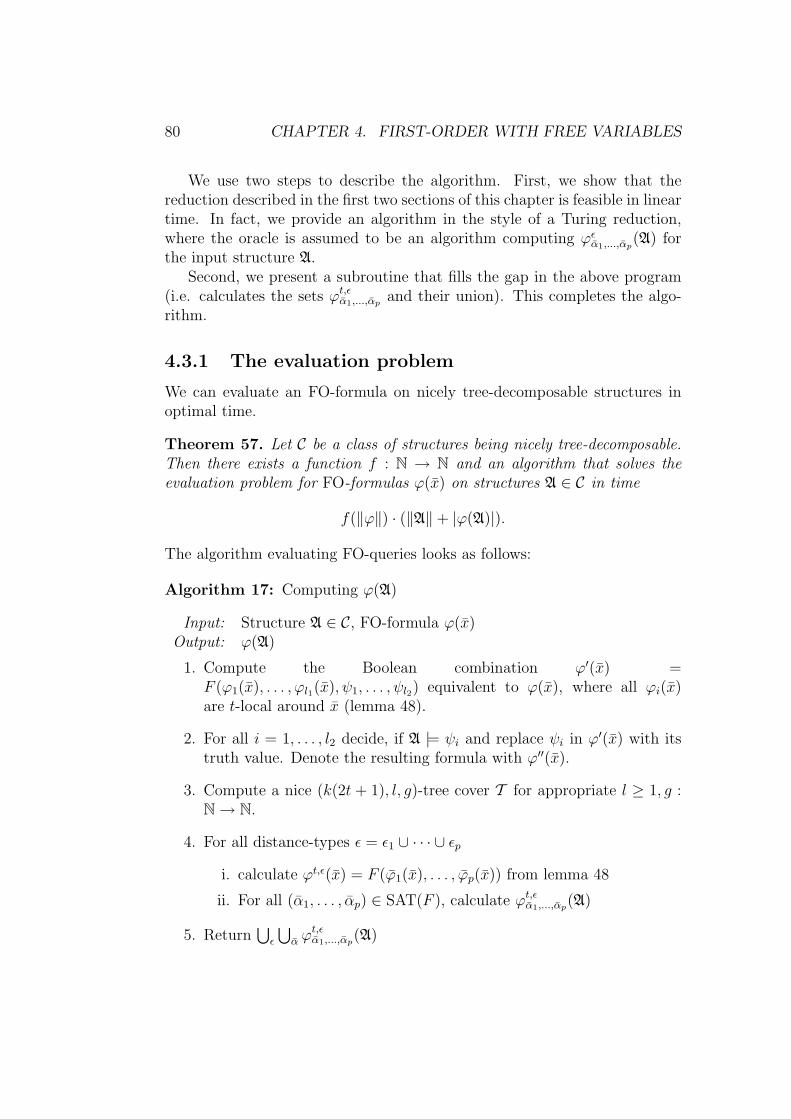
80 CHAPTER 4. FIRST-ORDER WITH FREE VARIABLES
We use two steps to describe the algorithm. First, we show that thereduction described in the first two sections of this chapter is feasible in lineartime. In fact, we provide an algorithm in the style of a Turing reduction,where the oracle is assumed to be an algorithm computing ϕεα1,...,αp
(A) forthe input structure A.
Second, we present a subroutine that fills the gap in the above program(i.e. calculates the sets ϕt,εα1,...,αp and their union). This completes the algo-rithm.
4.3.1 The evaluation problem
We can evaluate an FO-formula on nicely tree-decomposable structures inoptimal time.
Theorem 57. Let C be a class of structures being nicely tree-decomposable.Then there exists a function f : N → N and an algorithm that solves theevaluation problem for FO-formulas ϕ(x) on structures A ∈ C in time
f(‖ϕ‖) · (‖A‖+ |ϕ(A)|).
The algorithm evaluating FO-queries looks as follows:
Algorithm 17: Computing ϕ(A)
Input: Structure A ∈ C, FO-formula ϕ(x)Output: ϕ(A)
1. Compute the Boolean combination ϕ′(x) =F (ϕ1(x), . . . , ϕl1(x), ψ1, . . . , ψl2) equivalent to ϕ(x), where all ϕi(x)are t-local around x (lemma 48).
2. For all i = 1, . . . , l2 decide, if A |= ψi and replace ψi in ϕ′(x) with itstruth value. Denote the resulting formula with ϕ′′(x).
3. Compute a nice (k(2t + 1), l, g)-tree cover T for appropriate l ≥ 1, g :N→ N.
4. For all distance-types ε = ε1 ∪ · · · ∪ εp
i. calculate ϕt,ε(x) = F (ϕ1(x), . . . , ϕp(x)) from lemma 48
ii. For all (α1, . . . , αp) ∈ SAT(F ), calculate ϕt,εα1,...,αp(A)
5. Return⋃ε
⋃α ϕ
t,εα1,...,αp(A)

4.3. THE EVALUATION- AND WITNESS PROBLEM 81
The first line needs time linear in ‖ϕ′(x)‖, which itself only depends on‖ϕ(x)‖ (cf. the end of section 4.1, where we explained how to calculate thenormal form from lemma 48).
By definition, a nice (k(2t + 1), l, g)-tree cover can be computed in timeO(|A|), the same holds for the decision of A |= χi (by theorem 47). Thusline 2 and line 3 need time linear in the structure size.
The loop in line 4 is the crucial one. First, the number of different ε isconstant (depends only on k). Calculating ϕt,ε(x) needs time only dependingon ‖ϕ‖, and the number of different Boolean assignments (α1, . . . , αp) whichhave to be considered is also bounded by a constant. Hence, the subroutinecalculating ϕt,εα1,...,αp(A) is called constantly often.
By a result, being proved later on, ϕt,εα1,...,αp(A) can be calculated in time
O(|ϕ(A)|) (actually in time O(|ϕt,εα1,...,αp(A)|)), hence the entire loop is per-formed in time O(
∑ε
∑α |ϕ(A)|) = O(|ϕ(A)|). The last step, finally, outputs
the just computed sets.
Enumerating independent tuples: Consider the assumptions in algo-rithm 17 before the call of the subroutine in line 4ii, which does the maincomputation. That is, we have given a formula ϕ(x) of the form ϕt,εα1,...,αp(x)(recall formula 4.7), and a tree cover T of A. The procedure enum assign
that enumerates all tuples a such that A |= ϕ(a) is displayed as algorithm18.
Correctness: enum assign first calculates G := c(T , κ) and then elimi-
nates all vertices J ∈ Cc(T ,κ)i with Aκi
J= ∅. Note that a Cartesian product
is empty if, and only if, one of its parts is empty. This means that wethrow away those indices that, in any case, do not contribute to the re-sult. Calling indep tuples(G) (displayed as algorithm 19) then computesthe set of independent tuples I (line 9), which directly provides the set⋃
(J1,...,Jq)∈I Aκ1
J1× · · · × A
κqJq
. This proves the correctness of the algorithm.
And as it will turn out, this, performed in a clever way, is enough to obtainan optimal time bound.
Running time: Concerning the running time, we have to go more intodetails: Note that the outermost loop over κ is passed through a constantnumber of times. Consider the first part between line 4 and line 8: bydefinition, Aκi
Ji= ∅ can be decided in the structure 〈UJi〉, which, by the
additional property of nice tree covers, has bounded treewidth (by g(|κi|), cf.lemma 56). Hence, we can apply the algorithm from theorem 23 and decideemptiness in time f ′(‖ϕ‖) · |UJi|, for some f ′ : N → N. Furthermore, eacha ∈ A is contained in at most l sets UJ , hence
∑Ji∈CGi
|UJi| ≤ l|ε(κi)| · |A|

82 CHAPTER 4. FIRST-ORDER WITH FREE VARIABLES
1 proc enum assign(T , ϕ(x))2 for κ a p-contiguousness-type do3 G := c(T , κ);4 for i = 1 to q do5 for J ∈ CGi do6 if Aκi
J= ∅ then G := G \ J fi
7 od8 od9 I := indep tuples(G);
10 for i = 1 to q do11 Ii := I i;12 for J ∈ Ii do13 calculate Aκi
J;
14 od15 od16 B := ∅;17 for (J1, . . . , Jq) ∈ I do18 B := B ∪ Aκ1
J1× · · · × Aκq
Jq;
19 od20 od21 return(B);22 .
Algorithm 18. Evaluating a t-local formula
for all i ∈ [q]. Therefore, the running time for this loop is linear in the sizeof A. From now on, G denotes the graph after removing these “superflous”vertices.
In line 9, we call the function indep tuples(G) (algorithm 19) to computethe set of independent tuples of G.
Claim: indep tuples(G) returns all independent tuples of G and needs timeO(|indep tuples(G)|).
Proof of the Claim: Consider algorithm 19 and assume that G has maximaldegree d (it is an induced subgraph of a contiguousness-graph). In a firstloop, we partition the set of indices into “big” and “small” ones (lines 4 to8). The actual computation proceeds in two steps. In the first step, we lookexhaustively for all independent tuples over small indices (note that thereare at most (2dq)q many of them).

4.3. THE EVALUATION- AND WITNESS PROBLEM 83
1 proc indep tuples(G)2 I := ∅;3 d := max-degree(G); big = NULL; small = NULL;4 for i = 1 to q do5 if |CGi | > 2dq6 then append(big, i) else append(small, i)7 fi8 od9 if small = NULL
10 then11 Is := () else12 Is := all independent v ∈
∏i∈smallC
Gi
13 fi14 for v ∈ Is do15 for u ∈
∏i∈big C
Gi
16 if (v, u) independent17 then I := I ∪ (v, u)18 fi19 od20 od21 return(I);22 .
Algorithm 19. Calculate all independent tuples
Then, in the second step, we extend these “partial” tuples to tuples over[q], which gives the sought result. The code should be clear.
Let us estimate the time necessary for the second part of the search (thefirst part trivially needs constant time): for simplicity, we assume that allindices are big; the set of all possible tuples of indices (J1, . . . , Jq) has size∏q
i=1 |CGi |. A lower bound for the number of independent tuples is easily seen
to be |CG1 | · (|CG2 | − d) · · · (|CGq | − (q − 1)d). Since our loop goes through all
tuples in∏q
i=1 CGi , it is enough to show that there is a c > 0 (actually, we
choose c := 2q) such that
q∏i=1
|Ci| ≤ c ·q∏i=1
(|Ci| − dq).
To prove this, observe that by |Ci| > 2dq we have |Ci| ≤ 2 · (|Ci| − dq).

84 CHAPTER 4. FIRST-ORDER WITH FREE VARIABLES
Applied to the above situation we get
q∏i=1
|Ci| ≤ 2(|C1| − dq) ·q∏i=2
|Ci| ≤ · · · ≤ 2qq∏i=1
(|Ci| − dq)
as an upper bound on the number of times the loop (between lines 14 and20) is passed. Checking, if a tuple (J1, . . . , Jq) is independent can be donein constant time (a simple lookup in q adjacency lists, all of constant size).Together, we need time
∏qi=1 |C
Gi | = O(
∏qi=1(|Ci| − dq)). 2
So let us revert to the analysis of the running time of enum assign.We just computed the set I of independent tuples of G = c(T , κ) in timeO(|I|) (line 9). Because Aκi
J6= ∅, for all J ∈ CGi , the set I has at most∑
(J1,...,Jq)∈I |Aκ1
J1× · · · × Aκq
Jq| = O(|ϕ(A)|) elements. Hence the loop needs
O(|ϕ(A)|) time.
Now consider the subsequent loop for each i (lines 10 to 15): first, wecalculate the projection of I onto coordinate i. This can be done in O(|I|)steps. A bit more involved, and actually the reason for the first simplifica-tions is the loop over Ii. Observe that Aκi
Jican be calculated in 〈UJi〉. This
substructure has bounded treewidth (recall the first loop), thus we can cal-culate Aκi
Jiin time O(|UJi|+ |A
κiJi|) (recall theorem 21). Hence, the entire loop
requires ∑Ji∈Ii
(|UJi|+ |A
κiJi|))
= O(|A|+∑Ji∈Ii
|AκiJi|)
steps (for the equality, cf. the first loop). It remains to show that∑Ji∈Ii |A
κiJi| = O(|ϕ(A)|). For a tuple b define I(b) := Ji | b ∈ UJi the
number of times a b is computed. Assume Ji ∈ I(b). This entails for allν : Ji ∩ J | bν ∈ UJ 6= ∅, hence
|I(b)| ≤(|κi| · l|ε(κi)|
)|κi|.
Thus, each tuple occurring in⋃Ji∈Ii A
κiJi
is computed at most a constantnumber times, i.e. ∑
Ji∈Ii
|AκiJi| ≤
(|κi| · l|ε(κi)|
)|κi| · | ⋃Ji∈Ii
AκiJi|.
The same argument gives us: I = O(|ϕ(A)|). Finally, we injectively mapeach b ∈
⋃Ji∈Ii A
κiJi
to the lexicographically minimal a ∈ ϕ(A) such that
b = a ε(κi), hence the last term is O(|ϕ(A)|). Such a minimal a exists,
4.3. THE EVALUATION- AND WITNESS PROBLEM 85
since (i) we removed all Ji with empty AκiJi
and (ii) in Ii there are only
indices, which are part of an independent tuple (actually, this was the reasonfor calculating the projections Ii). For else, we would possibly compute“big” sets Aκi
Jithat do not contribute to ϕ(A) (because Ji is not part of a
independent tuple).
To finish, we sum up the times we just estimated. We have c1 · |A| for thefirst loop, and O(|ϕ(A)|) for the second one. As we have seen, the last twoloops need time O(|ϕ(A)|). This amounts to O(‖A‖+ |ϕ(A)|), as claimed inthe theorem. 2
4.3.2 Finding a witnessing tuple
The task of finding a witness for a formula reduces to the task of findingan independent tuple (J1, . . . , Jq) in the contiguousness graph c(T , κ) forsome κ. We describe a pigeonhole-like trick, which immediately provides thealgorithm.
Theorem 58. Let C be a class of nicely tree-decomposable structures. Thenthere is a function f : N → N and an algorithm that solves the witnessproblem for FO-formulas ϕ(x) on structures A ∈ C in time
f(‖ϕ‖) · ‖A‖.
Proof: The algorithm resembles very much the one of the evaluation case.It is displayed as algorithm 20. The analysis of the evaluation case showsthat step 1 to step 3 can be done in linear time. For the last step, assumethat, given a tree cover T , and a formula of the form ϕt,εα1,...,αq(x), we find awitness in linear time. Then the entire algorithm works in linear time (againby the already known fact that there are only constantly many different εand corresponding Boolean assignments α).
Algorithm 20: Computing an a ∈ ϕ(A)
Input: Structure A ∈ C, FO-formula ϕ(x)Output: an a with A |= ϕ(a)

86 CHAPTER 4. FIRST-ORDER WITH FREE VARIABLES
1. Compute the Boolean combination ϕ′(x) =F (ϕ1(x), . . . , ϕl1(x), ψ1, . . . , ψl2) equivalent to ϕ(x), where all ϕi(x)are t-local around x.
2. For all i = 1, . . . , l2 decide, if A |= ψi and replace ψi in ϕ′(x) with itstruth value. Denote the resulting formula with ϕ′′(x).
3. Compute a nice (k(2t + 1), l, g)-tree cover T for appropriate l ≥ 1, g :N→ N.
4. For all distance-types ε = ε1 ∪ · · · ∪ εp
i. calculate ϕt,ε(x) = F (ϕ1(x), . . . , ϕp(x)) from lemma 48
ii. For all (α1, . . . , αp) ∈ SAT(F ), calculate a witness for ϕt,εα1,...,αp(x)in A
5. return one of the found witnesses, if it exists
So it remains to show that finding a witness for formulas of the specialform ϕt,εα (x) can be done in linear time. We already saw in the evaluation casethat satisfying tuples roughly correspond to independent tuples in the con-tiguousness graph. Fortunately, in graphs of bounded valence, independenttuples are easy to find.
Lemma 59. Let (G, C1, . . . , Cq) be a q-colored graph with maximal degreed. Then there is an algorithm that finds an independent tuple (v1, . . . , vq) ∈∏q
i=1 CGi in linear time.
Proof: At the beginning, the subroutine partitions the colors into “big” and“small” ones. The point is that small colors have constant size, hence we cantry all possibilities to find a partial independent tuple. On the other hand,big colors are sufficiently big that, by any means, there exists an extensionof the formerly found partial independent tuple.
The subroutine indep tuple is displayed as algorithm 21. Lines 2 to 8 dothe partitioning. Then the routine exhaustively searches for an independenttuple in the subgraph induced by
⋃i∈smallC
Gi . Obviously, this requires ≤
O((d · q)q) steps. The following claim is the key to the correctness of thealgorithm:
Claim: If u is an independent tuple in 〈⋃i∈smallC
Gi 〉, then line 15 to 23
expand u to an independent tuple of G.
Proof of the claim: Observe that i ≤ q vertices in G have together at mostd · i neighbors. Of each “big” color there are more than d · q vertices, thus
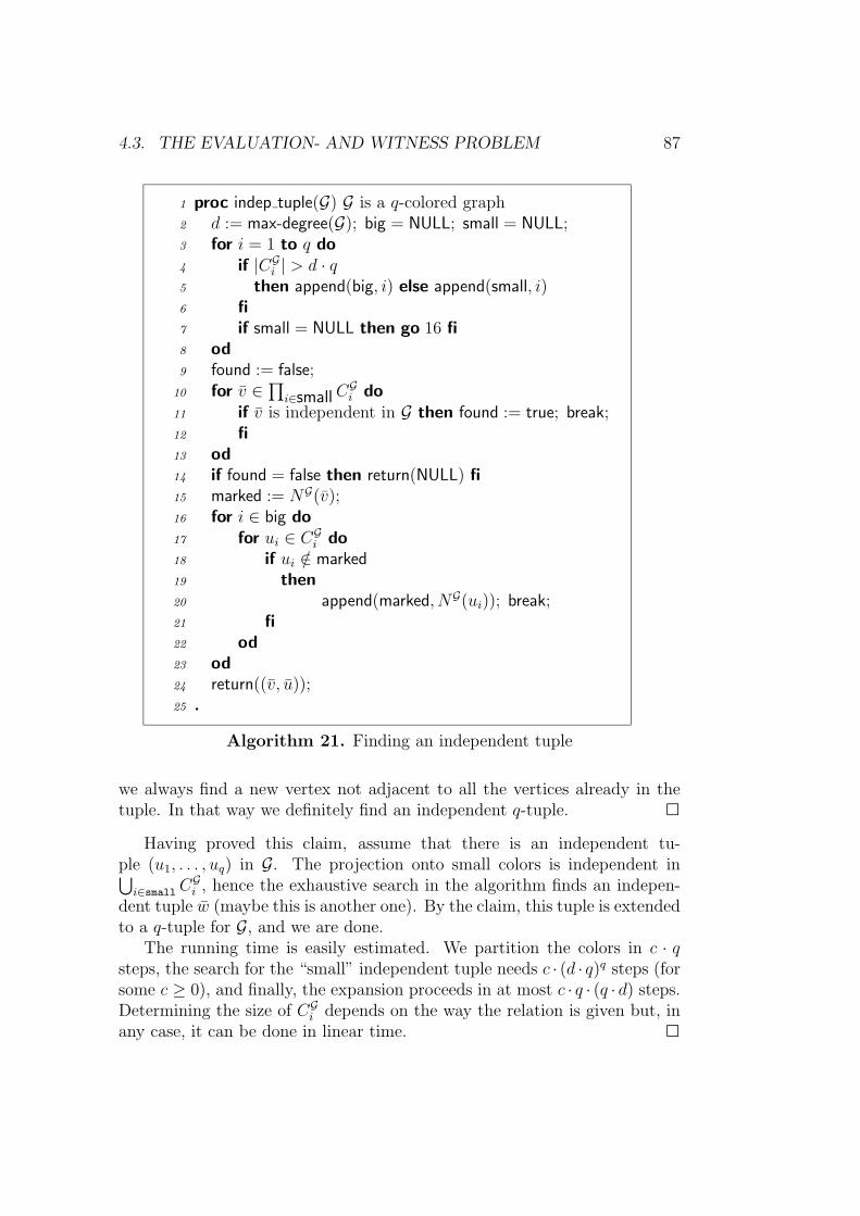
4.3. THE EVALUATION- AND WITNESS PROBLEM 87
1 proc indep tuple(G) G is a q-colored graph2 d := max-degree(G); big = NULL; small = NULL;3 for i = 1 to q do4 if |CGi | > d · q5 then append(big, i) else append(small, i)6 fi7 if small = NULL then go 16 fi8 od9 found := false;
10 for v ∈∏
i∈smallCGi do
11 if v is independent in G then found := true; break;12 fi13 od14 if found = false then return(NULL) fi15 marked := NG(v);16 for i ∈ big do17 for ui ∈ CGi do18 if ui /∈ marked19 then20 append(marked, NG(ui)); break;21 fi22 od23 od24 return((v, u));25 .
Algorithm 21. Finding an independent tuple
we always find a new vertex not adjacent to all the vertices already in thetuple. In that way we definitely find an independent q-tuple. 2
Having proved this claim, assume that there is an independent tu-ple (u1, . . . , uq) in G. The projection onto small colors is independent in⋃i∈smallC
Gi , hence the exhaustive search in the algorithm finds an indepen-
dent tuple w (maybe this is another one). By the claim, this tuple is extendedto a q-tuple for G, and we are done.
The running time is easily estimated. We partition the colors in c · qsteps, the search for the “small” independent tuple needs c · (d · q)q steps (forsome c ≥ 0), and finally, the expansion proceeds in at most c · q · (q · d) steps.Determining the size of CGi depends on the way the relation is given but, inany case, it can be done in linear time. 2

88 CHAPTER 4. FIRST-ORDER WITH FREE VARIABLES
We now turn to the routine that finds a witnessing tuple for ϕt,εα1,...,αp(x).This subroutine is displayed as algorithm 22. The correctness ofwitness assign is obvious.
1 proc witness assign(T , ϕ(x))2 for κ a p-contiguousness-type do3 G := c(T , κ);4 for i = 1 to q do5 for J ∈ CGi do6 if Aκi
J= ∅ then G := G \ J fi
7 od8 od9 (J1, . . . , Jq) := indep tuple(G);
10 if (J1, . . . , Jq) 6= NULL11 then12 calculate an a ∈
∏qi=1 A
κiJi
13 return(a)14 fi15 od16 return(NULL);17 .
Algorithm 22. Finding a witness
Concerning the running time, recall that the first loop needs linear time(cf. evaluation case). Then, by a subroutine call, we determine an indepen-dent tuple (J1, . . . , Jq) (if one exists!). The last step calculates a represen-tative ai ∈ Aκi
Ji, for each i ≤ q. By theorem 22, this requires linear time.
Altogether, we stay within linear time. 2
4.4 The counting problem
The last problem remaining open for first-order formulas over nicely tree-decomposable structures is counting the number of satisfying assignments.We proceed in two steps. In the first one, we reduce the counting problemto the calculation of a sum over integers associated with independent sets ofa graph. Then, in the last section, we show how this sum can be evaluatedquickly.
Remember that, in the context of counting algorithms, we assume thatarithmetical operations can be done in constant time. Like before we reduce

4.4. THE COUNTING PROBLEM 89
the question for an FO-formula ϕ(x) to the case where ϕ(x) is of the formϕt,εα1,...,αp(x) for a k-distance-type ε = ε1 ∪ · · · ∪ εp, the locality rank t of ϕ(x),and a fitting Boolean assignment (α1, . . . , αp). Recall formula (4.6) on page71:
ϕ(A) =⋃ε
⋃(α1,...,αp)
ϕt,εα1,...,αp(A). (4.13)
This union goes over disjoint sets, hence
|ϕ(A)| =∑ε
∑(α1,...,αp)
|ϕt,εα1,...,αp(A)|.
This immediately leads to algorithm 4.4 for the counting problem, leavingopen how to calculate the values |ϕt,εα1,...,αp(A)| of the double sum. The linesuntil line 3 are already familiar. After that, we simply cycle over all possibleε and fitting α, and sum up the respective |ϕt,εα1,...,αp(A)|.
Algorithm 23: Computing |ϕ(A)|
Input: Structure A ∈ C, FO-formula ϕ(x)Output: |ϕ(A)|
1. Compute the Boolean combination ϕ′(x) =F (ϕ1(x), . . . , ϕl1(x), ψ1, . . . , ψl2) equivalent to ϕ(x), where all ϕi(x)are t-local around x.
2. For all i = 1, . . . , l2 decide, if A |= ψi and replace ψi in ϕ′(x) with itstruth value. Denote the resulting formula with ϕ′′(x).
3. Compute a nice (k(2t + 1), l, g)-tree cover T for appropriate l ≥ 1, g :N→ N.
4. For all distance-types ε = ε1 ∪ · · · ∪ εp
i. calculate ϕt,ε(x) = F (ϕ1(x), . . . , ϕp(x)) (cf. 48)
ii. for all (α1, . . . , αp) ∈ SAT(F ), calculate γεα := |ϕt,εα1,...,αp(A)|
5. Return∑
ε
∑α γ
εα
Like in the algorithm for the evaluation problem the lines until line 3 needlinear time. The subsequent loop goes over a constant number of distancetypes ε and respective Boolean assignments α. Hence, assuming that γεα canbe computed in linear time, we are done. 2
This algorithm, together with theorem 67 (in the next subsection), whichallows us to evaluate the double sum, yield the intended counting result:

90 CHAPTER 4. FIRST-ORDER WITH FREE VARIABLES
Theorem 60. Let C be a class of nicely tree-decomposable structures. Thenthere is a function f : N → N and an algorithm that solves the countingproblem for FO-formulas ϕ(x) on structures A ∈ C in time
f(‖ϕ‖) · ‖A‖.
4.4.1 Reducing the starting problem
In the sequel, let ϕ(x) be of the form ϕt,εα1,...,αp(x) for t being the locality rankof ϕ, a distance type ε with components ε1, . . . , εp, together with a suitableBoolean assignment (α1, . . . , αp). k denotes the number of free variables ofϕ(x) and T = U1, . . . , Um is a nice (r, l, g)-tree cover for A.
We will develop a procedure that involves two steps: First, we reduce theproblem of computing |ϕ(A)| to computing a sum over the independent tuplesof a q-colored graph G. Essentially, this sum will look as follows:
γ =∑
v independentvi∈Ci
γ(v1) · · · γ(vq),
where γ(v) is an integer attached to vertex v in the graph G. This reductionis described in the next section, which resembles the evaluation case, but isa bit more complicated. In particular, we give an algorithm that calculatesthe graph G (an extension of the contiguousness graph c(T , κ) from section4.2) and the labels γ(v). The section ends with a procedure that calculatesthe above sum in linear time, completing the proof of theorem 60.
Let us start with the first part. The following equation characterizes thecardinality of ϕ(A) and is a consequence of equation (4.8) on page 74 andthe principle of inclusion and exclusion (PIE). We define AJ :=
⋂J∈J AJ for
an arbitrary index set J .
|ϕ(A)| = |⋃
(J1,...,Jp)∈[m]p
AJ1,...,Jp |PIE=
∑∅6=J⊆[m]p
(−1)|J |+1|AJ | (4.14)
It is worthwhile to compare the situation with the one we had in the evalua-tion case. After including the tree cover into equation (4.8) we grouped theindices (J1, . . . , Jp) with respect to their mutual dependence in the computa-tion of AJ1,...,Jp (cf. lemma 50). In the present case this looks more difficult,because now we have sets of tuples, which apparently lost the relevant topo-logical information.

4.4. THE COUNTING PROBLEM 91
To circumvent this problem, we pass from sets of indices to their projec-tions. More formally, for ∅ 6= J ⊆ [m]p we define J j := Jj | there is a(J1, . . . , Jj, . . . , Jp) ∈ J , the projection of J onto coordinate j.
The natural extension of the definition of AJ1,...,Jp (4.9) to sets of indicesrelates these projections to the sets AJ . We set
AJ1,...,Jp := AJ1×···×Jp ,
which receives further justification by the next lemma, stating that Cartesianproduct and projection are inverse to each other.
Lemma 61. With the above notation, the following holds for all J ⊆ [m]p:
AJ = AJ1,...,Jp.
Proof: The sets on both sides only contain tuples a with A |= ϕ(a), hence itis not necessary to state that explicitly, and we can restrict the argumentationon the requirements imposed by the index sets.
Now, let be J ⊆ [m]p and a ∈ AJ . By definition, this is equivalent toa εi ∩Kr(UJi) 6= ∅ for all i = 1, . . . , p and all (J1, . . . , Jp) ∈ J . The sameholds for all (J1, . . . , Jp) ∈ J 1 × · · · × J p. The backward direction istrivial because J ⊆ J 1× · · · × J p implies AJ ⊇ AJ1,...,Jp. 2
We rewrite equation (4.14) as follows:
|ϕ(A)| =mp∑j=1
(−1)j+1∑
J⊆[m]p,|J |=j
|AJ |
=mp∑j=1
(−1)j+1∑
J1,...,Jp⊆[m]
∑J ,|J |=jJi=Ji
|AJ |. (4.15)
To examine the last equation fix some 1 ≤ j ≤ mp and index setsJ1, . . . ,Jp ⊆ [m]. We claim that the number of addends of the inner-most sum (the sum over the sets J ⊆ [m]p) only depends on the sizesm1 := |J1|, . . . ,mp := |Jp| and j. Thereto, take new index sets J ′i ⊆ [m] withmi = |J ′i | for i = 1, . . . , p. By assumption, there are bijections βi : Ji → J ′i .These bijections lead to a bijection β from the admitted sets for J1, . . . ,Jpto the admitted sets for J ′1, . . . ,J ′p by the following definition:
β : J 7→ (β1(J1), . . . , βp(Jp)) | (J1, . . . , Jp) ∈ J .
Observe that this mapping preserves the size, i.e. |J | = |β(J )|. If we denotethe number of sets J with |J | = j and |J i| = mi by µj(m1, . . . ,mp), i.e.
µj(m1, . . . ,mp) := |J ⊆ [m]p | |J i| = mi, i = 1, . . . , p and |J | = j|,
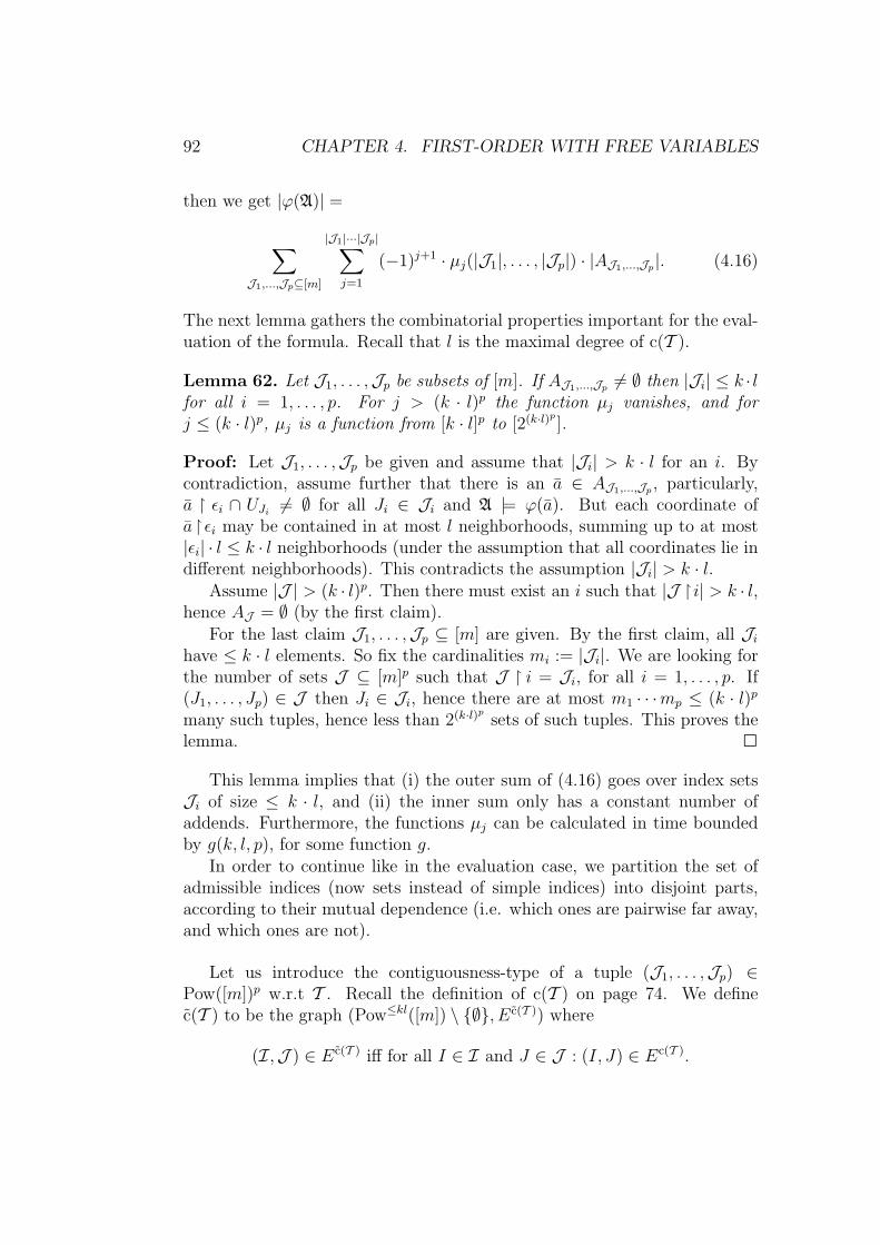
92 CHAPTER 4. FIRST-ORDER WITH FREE VARIABLES
then we get |ϕ(A)| =
∑J1,...,Jp⊆[m]
|J1|···|Jp|∑j=1
(−1)j+1 · µj(|J1|, . . . , |Jp|) · |AJ1,...,Jp |. (4.16)
The next lemma gathers the combinatorial properties important for the eval-uation of the formula. Recall that l is the maximal degree of c(T ).
Lemma 62. Let J1, . . . ,Jp be subsets of [m]. If AJ1,...,Jp 6= ∅ then |Ji| ≤ k · lfor all i = 1, . . . , p. For j > (k · l)p the function µj vanishes, and forj ≤ (k · l)p, µj is a function from [k · l]p to [2(k·l)p ].
Proof: Let J1, . . . ,Jp be given and assume that |Ji| > k · l for an i. Bycontradiction, assume further that there is an a ∈ AJ1,...,Jp , particularly,a εi ∩ UJi 6= ∅ for all Ji ∈ Ji and A |= ϕ(a). But each coordinate ofa εi may be contained in at most l neighborhoods, summing up to at most|εi| · l ≤ k · l neighborhoods (under the assumption that all coordinates lie indifferent neighborhoods). This contradicts the assumption |Ji| > k · l.
Assume |J | > (k · l)p. Then there must exist an i such that |J i| > k · l,hence AJ = ∅ (by the first claim).
For the last claim J1, . . . ,Jp ⊆ [m] are given. By the first claim, all Jihave ≤ k · l elements. So fix the cardinalities mi := |Ji|. We are looking forthe number of sets J ⊆ [m]p such that J i = Ji, for all i = 1, . . . , p. If(J1, . . . , Jp) ∈ J then Ji ∈ Ji, hence there are at most m1 · · ·mp ≤ (k · l)pmany such tuples, hence less than 2(k·l)p sets of such tuples. This proves thelemma. 2
This lemma implies that (i) the outer sum of (4.16) goes over index setsJi of size ≤ k · l, and (ii) the inner sum only has a constant number ofaddends. Furthermore, the functions µj can be calculated in time boundedby g(k, l, p), for some function g.
In order to continue like in the evaluation case, we partition the set ofadmissible indices (now sets instead of simple indices) into disjoint parts,according to their mutual dependence (i.e. which ones are pairwise far away,and which ones are not).
Let us introduce the contiguousness-type of a tuple (J1, . . . ,Jp) ∈Pow([m])p w.r.t T . Recall the definition of c(T ) on page 74. We definec(T ) to be the graph (Pow≤kl([m]) \ ∅, E c(T )) where
(I,J ) ∈ E c(T ) iff for all I ∈ I and J ∈ J : (I, J) ∈ Ec(T ).
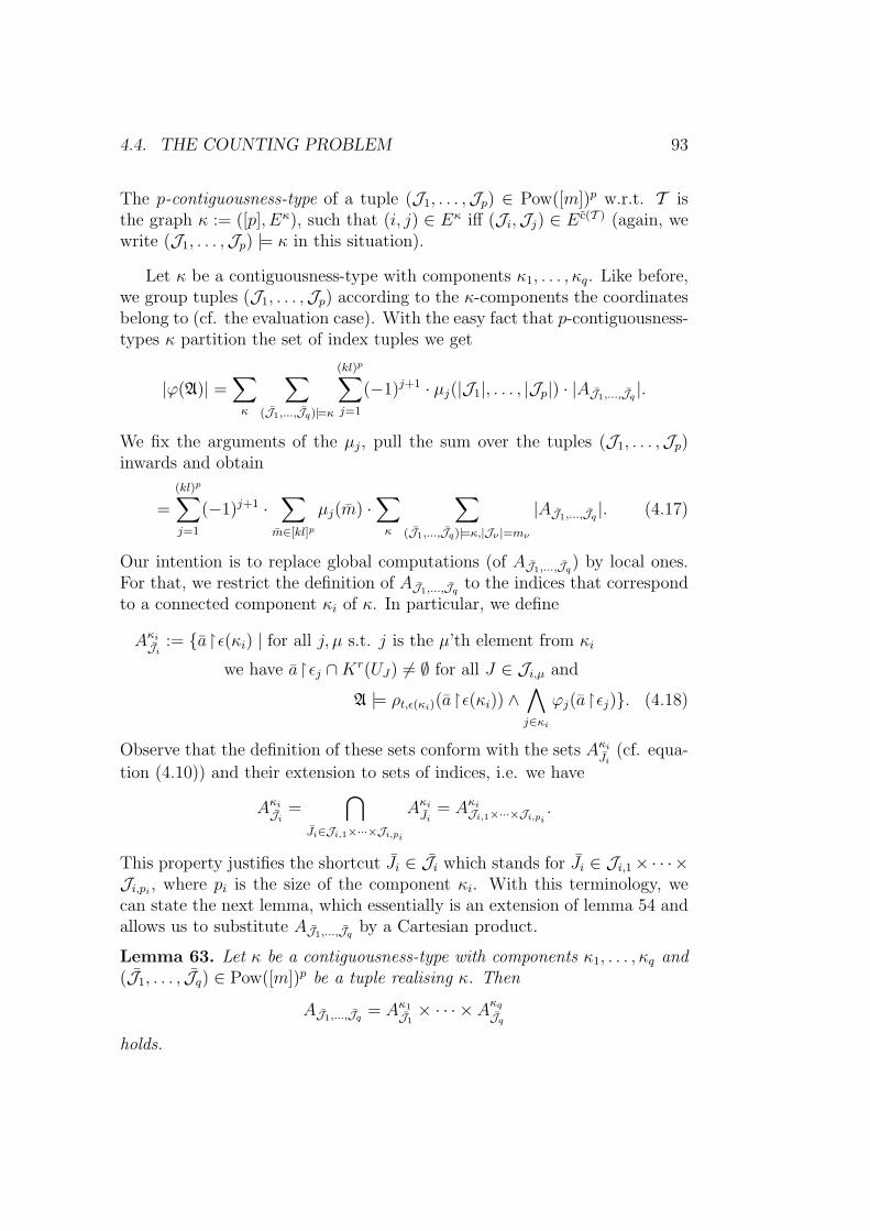
4.4. THE COUNTING PROBLEM 93
The p-contiguousness-type of a tuple (J1, . . . ,Jp) ∈ Pow([m])p w.r.t. T isthe graph κ := ([p], Eκ), such that (i, j) ∈ Eκ iff (Ji,Jj) ∈ E c(T ) (again, wewrite (J1, . . . ,Jp) |= κ in this situation).
Let κ be a contiguousness-type with components κ1, . . . , κq. Like before,we group tuples (J1, . . . ,Jp) according to the κ-components the coordinatesbelong to (cf. the evaluation case). With the easy fact that p-contiguousness-types κ partition the set of index tuples we get
|ϕ(A)| =∑κ
∑(J1,...,Jq)|=κ
(kl)p∑j=1
(−1)j+1 · µj(|J1|, . . . , |Jp|) · |AJ1,...,Jq |.
We fix the arguments of the µj, pull the sum over the tuples (J1, . . . ,Jp)inwards and obtain
=
(kl)p∑j=1
(−1)j+1 ·∑
m∈[kl]p
µj(m) ·∑κ
∑(J1,...,Jq)|=κ,|Jν |=mν
|AJ1,...,Jq |. (4.17)
Our intention is to replace global computations (of AJ1,...,Jq) by local ones.For that, we restrict the definition of AJ1,...,Jq to the indices that correspondto a connected component κi of κ. In particular, we define
AκiJi := aε(κi) | for all j, µ s.t. j is the µ’th element from κi
we have aεj ∩Kr(UJ) 6= ∅ for all J ∈ Ji,µ and
A |= ρt,ε(κi)(aε(κi)) ∧∧j∈κi
ϕj(aεj). (4.18)
Observe that the definition of these sets conform with the sets AκiJi
(cf. equa-
tion (4.10)) and their extension to sets of indices, i.e. we have
AκiJi =⋂
Ji∈Ji,1×···×Ji,pi
AκiJi
= AκiJi,1×···×Ji,pi.
This property justifies the shortcut Ji ∈ Ji which stands for Ji ∈ Ji,1×· · ·×Ji,pi , where pi is the size of the component κi. With this terminology, wecan state the next lemma, which essentially is an extension of lemma 54 andallows us to substitute AJ1,...,Jq by a Cartesian product.
Lemma 63. Let κ be a contiguousness-type with components κ1, . . . , κq and(J1, . . . , Jq) ∈ Pow([m])p be a tuple realising κ. Then
AJ1,...,Jq = Aκ1
J1× · · · × AκqJq
holds.

94 CHAPTER 4. FIRST-ORDER WITH FREE VARIABLES
Proof: To prove the lemma we reduce the problem to the case where wehave indices instead of sets of indices (as in lemma 54). Thereto recall that,by definition, we have
AJ1,...,Jq := AJ1×···×Jq =⋂
J1,...,Jq∈J1×···×Jq
AJ1,...,Jq .
For arbitrary (J1, . . . , Jq) ∈ J1 × · · · × Jq we have (J1, . . . , Jq) |= κ (bydefinition). For such tuples, lemma 54 yields AJ1,...,Jq = Aκ1
J1× · · · × A
κqJq
,
hence
AJ1,...,Jq =⋂
(J1,...,Jq)∈J1×···×Jq
Aκ1
J1× · · · × Aκq
Jq=⋂J1∈J1
Aκ1
J1× · · · ×
⋂Jq∈Jq
AκqJq,
which is equal to Aκ1
J1× · · · × AκqJq . 2
In the sequel, we treat sets of the form AκiJi . These sets are empty, if at
least for one of the indices Ji,ν we have: UJi,ν = ∅. Since these sets do notcontribute to the result, we omit them, i.e. if (J1, . . . , Jq) |= κ, we implicitlyassume that UJi 6= ∅ for i = 1, . . . , p. Later, we will see that this restrictionhas crucial impact on the tractability of c(T ).
With the above lemma, equation (4.17) can be transformed to
=
(kl)p∑j
(−1)j+1∑
m∈[kl]p
µj(m) ·∑κ
∑(J1,...,Jq)|=κ,|Jν |=mν
|Aκ1
J1| · · · |AκqJq |. (4.19)
Since the outer sums have a constant number of addends and µj can be cal-culated easily, this characterization of |ϕ(A)| gives us immediatly a reductionof the starting problem to the calculation of
γ(m, κ) :=∑
(J1,...,Jq)|=κ,|Jν |=mν
|Aκ1
J1| · · · |AκqJq |. (4.20)
4.4.2 Counting
In this last section, we show how to calculate the value
γ(m, κ) :=∑
(J1,...,Jq)|=κ,|Jν |=mν
|Aκ1
J1| · · · |AκqJq | (4.21)
in linear time. Therefore, like in the evaluation case, we translate this ques-tion to a graph theoretic one. What follows is a slight variation of section

4.4. THE COUNTING PROBLEM 95
4.2.1. Let T = U1, . . . , Um be a nice (r, l, g)-tree cover. For a contiguous-ness graph κ and m ∈ [k · l]p define PModT (κ, m) := J | J |= κ, UJi 6=∅ and |Ji| = mi. This is the obvious extension of ModT (κ) to the presentcase.
Definition 64. Let κ be a p-contiguousness-type with components κ1, . . . , κqand (m1, . . . mq) ∈ [k · l]p. The contiguousness graph c(T , κ, m) of T with
respect to κ and m has vertex set PModT (κ1, m1)·∪ · · ·
·∪PModT (κq, mq) and
edge relation E c(T ,κ,m) defined as follows:
(Ji, Jj) ∈ E c(T ,κ,m) iff there are ν, µ : (Ji,ν ,Jj,µ) ∈ E c(T ).
Additionally, we give the vertices corresponding to PModT (κi, mi) the color
i or, more formally, we add unary relations C1, . . . , Cq with Cc(T ,κ,m)i :=
PModT (κi, mi).
The next lemma corresponds to lemma 56 and gathers the relevant prop-erties of contiguousness graphs c(T , κ, m) for a tree cover T .
Lemma 65. Let T be an (r, l, g)-tree cover of a structure A. Then for all κand m ∈ [k · l]p:
(1) c(T , κ, m) can be calculated in time O(|T |).
(2) c(T , κ, m) has maximal degree bounded by some function on l.
Proof: To prove (1) we present an algorithm computing c(T , κ, m). In thefirst step we compute the graph c(T ) without the unnecessary vertices J(those for which UJ = ∅). This procedure is displayed as algorithm 24. Forthe correctness, note that if for J ⊆ [m] we have UJ 6= ∅, then there isa J ∈ J with J ⊆ N c(T )(J). Hence, we really get all relevant vertices ofc(T ). For the loop which generates the adjacency lists, note further thatI × J ⊆ Ec(T ) coincides with the definition of E c(T ). Furthermore, any twoadjacent I,J there must be I ∈ I and J ∈ J such that I and J are adjacentin c(T ).
It is easy to see that the running time is bounded by m · 2l · l · 2l · c wherec is the time necessary to check I ×J ⊆ Ec(T ) in a graph of bounded degree,given in adjacency list representation (this constant is independent from m).
To continue, recall algorithm 16, which calculates the contiguousnessgraph c(T , κ), and the definition of κi(J) for J ∈ [m] and 1 ≤ i ≤ q. Thisdefinition is naturally extended to
κi(J , m) := J ∈ PModT (κi, m) | J = Jj for some j.

96 CHAPTER 4. FIRST-ORDER WITH FREE VARIABLES
1 proc calc pgraph(T )2 for J = 1 to m do3 i := 1;4 for I ⊆ N c(T )(J) do5 vertex[i] := I; adj[i] := NULL;6 /* add adjacencies */7 for I ∈ N c(T )(J) do8 for J ⊆ N c(T )(I) do9 if I × J ⊆ Ec(T )
10 then11 append(adj[i],J );12 fi13 od14 od15 i := i+ 1;16 od17 od18 normalize the graph (vertex[·], adj[·]);19 .
Algorithm 24. Calculate c(T )
Algorithm 25 essentially works like algorithm 16, with roles of c(T ) and c(T )interchanged.
Correctness is immediate by the definition of the c(T , κ, m). For example,there is an edge between I and J iff there are µ,ν such that (Iν ,Jµ) ∈ E c(T ).The µ is delivered by the corresponding for-loop, and ν is implicit in theexpression I ∈ κl(I, ml) (the ν such that I = Iν). Finally I ∈ N c(T )(Jµ)assures that the tuples are adjacent.
For the running time, recall that J ∈ κi(J , mi) can be checked in con-stant time (cf. the case of primitive vertices). Thus, all loops except fromthe one cycling over J ∈ c(T ) are bounded by a constant of the form f(q, l)for a function f : N2 → N. Together, we get the running time dominated byf(q, l) · 2l ·m.
To prove (2), note that c(T ) has maximum degree 2l. Thus, |κi(J , mi)| ≤((2l)pi)pi−1 for a vertex J ∈ c(T ). Thus, summing up over all loops thatcompute the adjacency list, we get pi · q · 2l · ((2l)p)p−1 as an upper bound onthe degree (the maximal number of different I the algorithm can choose inthe loops between line 10 and line 18). 2
Finally, by the following lemma, we can assume the values |AκiJi| being

4.4. THE COUNTING PROBLEM 97
1 proc calc cgraph(T , κ)2 comment: calculate the vertex set3 for i = 1 to q do /* the colors */4 j := 1;5 for J ∈ c(T ) do6 for J ∈ κi(J , mi) do7 vertex[i, j] := J ;8 comment: calculate the adjacency list9 adj[i, j] := NULL;
10 for µ = 1 to pi do11 for l = 1 to q do12 for I ∈ N c(T )(Jµ) do13 for I ∈ κl(I, ml) do14 append(adj[i, j], I);15 od16 od17 od18 od19 j := j + 1;20 od21 od22 od23 normalize the graph (vertex[·, ·], adj[·, ·]);24 .
Algorithm 25. Calculate c(T , κ, m)
known. Observe that only here we really need that our tree covers are nice.
Lemma 66. The values |AκiJi| for i = 1, . . . , q and Ji ∈ C c(T ,κ,m) can becomputed in linear time.
Proof: We compute the |AκiJi| for all Ji ∈ Ci and fixed 1 ≤ i ≤ q straight-
forwardly by a simple loop over Ji and calls of the procedure from theorem23. For that, observe that |AκiJi| can be computed in the structure 〈UJ〉A for
an index J with Jν ∈ Ji,ν , for all ν. Furthermore, for an index J there are atmost (2l)|κi| many Ji satisfying this condition. Like before, since each indexJ is used constantly often, also each a ∈ A is contained constantly often ina set 〈UJ〉, hence the entire computation needs linear time. 2
Now it is easy to see that we are done, if we are able to evaluate theformula (4.21) in linear time. So fix an m ∈ [k · l]q and a contiguousness-type

98 CHAPTER 4. FIRST-ORDER WITH FREE VARIABLES
κ with components κ1, . . . , κq. Define G := c(T , κ, m) and set γ(Ji) := |AκiJi|for Ji ∈ CGi := PModT (κi, mi). Then the tuples (J1, . . . , Jq) ∈ CG1 ×· · ·×CGqadmitted in the sum are exactly the ones that are independent in G.
By lemma 65 the q-colored graph (G, C1, . . . , Cq) has degree bounded by,say, d ≥ 1. The next theorem fills the gap still missing in the proof of theorem60
Theorem 67. There is an algorithm that, given G as above, calculates thevalue
σ(G, γ) :=∑
(v1,...,vq) independent
γ(v1) · · · γ(vq) (4.22)
in time O(‖G‖).
If we plug in this algorithm into the gap left open in algorithm 4.4, thenthe counting problem for FO over classes that admit nice tree covers is solved.We assume the uniform cost measure for arithmetic operations on integers.To attack theorem 67 we need some new definitions.
Let G and a labelling γ be given as above. We group the tuples v accordingto the subgraph they induce in G. Fix a graph π over the set [q] and definethe subsets
Hom(π) := v | (i, j) ∈ Eπ ⇒ (vi, vj) ∈ EG
and
Iso(π) := v | (i, j) ∈ Eπ ⇔ (vi, vj) ∈ EG
of∏q
i=1 CGi . It is easy to see that v ∈ Iso(π) iff v ∈ Hom(π) and for all π′ ) π:
v /∈ Hom(π′). Using these index sets, we define cπ :=∑
v∈Hom(π)
∏i∈[q] γ(vi)
and dπ :=∑
v∈Iso(π)
∏i∈[q] γ(vi). It is easy to see that σ(G, γ) coincides with
dπ for π being the graph consisting of q isolated vertices.We start with a lemma that allows us to calculate the values cπ.
Lemma 68. Let π be a arbitrary graph over [q]. Then cπ can be calculatedin time O(qdq · ‖G‖), where d is the maximal degree of G.
Proof: Let π be a graph over [q] splitting up into components π1, . . . , πr. Bydefinition, we have cπ = cπ1 · · · cπr (just apply the distributive law). Henceit is enough to show that the claim holds for connected π.
So assume that π is connected and take an arbitrary j ∈ [q]. If v ∈Hom(π) then, by connectedness, vi ∈ NGq (v) ∩ Ci for all i 6= j. Since G hasdegree at most d, NGq (v) contains ≤ dq elements. Observe that the situation

4.4. THE COUNTING PROBLEM 99
is similar to that in lemma 56 where we calculated c(T , κ) for a tree cover Tand a contiguousness-type κ.
Now the algorithm proceeds as follows: In a first phase, using thejust derived characterization, we compute a list containing all tuples vthat are in Hom(π). This list may contain multiples. Then we removemultiple occurences from the list, and, in a last step, we sum up theγ(v) := γ(v1) · · · γ(vq) for v from the list. This is displayed as algorithm26.
1 proc calc pi(G, γ)2 comment: calculate the vertex set3 h := ∅; j ∈ [q];4 for v ∈ Cj do5 for v such that vj = v and all vi ∈ Nq(v) ∩ Ci do6 if v ∈ Hom(π) then7 append(h, v);8 fi9 od
10 od11 remove multiples from h;12 return(
∑v∈h γ(v1) · · · γ(vq))
13 .
Algorithm 26. Calculate cπ
It is easy to see that the algorithm works correctly. The time boundsare easily verified. For instance, the loops require time O(|G| · dq) (since|Nq(v)| ≤ dq). Multiple occurrences of tuples can be removed by a simpleRadix-sort (cf. the appendix) and the sum in the last line is computed intime linear in the size of h. 2
With this lemma we are almost finished. By the above observation onthe relation between homomorphisms and isomorphisms, we have
dπ = cπ −∑π′)π
dπ′ , (4.23)
which leads us to the following procedure:
Algorithm 27: Computing σ(G, γ)
Input: A graph (G, C1, . . . , Cq) and γ : G→ N
Output: σ(G, γ)
100 CHAPTER 4. FIRST-ORDER WITH FREE VARIABLES
1. Compute cπ for all π over [q]
2. Compute dπ for all π using formula (4.23)
3. Return dπ for π the empty graph
The correctness is immediate. Since there are ≤ 2q2
different π the firstline needs time O(‖G‖) (by lemma 68). Line 2 needs some more explanations:by induction, we proceed downwards starting with the complete graph π (forwhich we have cπ = dπ). Having computed all dπ for π with l + 1 edges, wecan compute dπ for π with l edges in constant time (simply using formula(4.23)).
Altogether we stay within the time bounds claimed in theorem 67. 2

Appendix A
The Machine Model
This appendix is dedicated to a detailed definition of the machine modelused. This is of particular interest, because linear time classes depend heavilyon the model, and still there is no agreement on which one is the mostappropriate. We will use Random Access Machines (RAM) that have aninfinite supply of registers, each of which may contain a natural number.
The choice for RAMs is motivated by the fact that most algorithms,considered to run in linear time, depend on pointers and direct access todata, a feature that is not provided by Turing machines. Essentially, thereare two ways to charge time for a single operation. The uniform time measurecharges one time unit for each operation, whatever the size of the involvedregisters is. In this framework, the content of a register is considered to haveconstant size. To some extend this model is justified by the fact that mostobjects in algorithms are represented by pointers, which in a real computerhave constant size.
In contrast to that, the logarithmic cost measure charges the logarithmof the values of the registers involved in the operation. This cost measurereflects the fact that logarithmic space is necessary to store numbers. Formost algorithms (that do not involve too much arithmetic) this difference isneglected because of the following reason: the collection of primitive inputobjects (e.g. the vertices of a graph) is assumed to be an initial segment ofthe natural numbers. This problem of normalized inputs will be addressedlater.
We slightly modify the model defined by Grandjean in a series of papers[Gra94a, Gra94b, Gra96]. This model is an extension of the basic RAM-model described in, for example, [CR73], based on the logarithmic cost mea-sure. We present the definition of the model in the first section. Then weaddress the problem of relational structures as inputs of machines, and its
101
102 APPENDIX A. THE MACHINE MODEL
impact on the model checking problem. There we encounter the problem ofnormalizing the input.
Finally we give some sample algorithms to illustrate the used pseudo-codeand frequently used data structures.
A.1 The Definition
The following definition of a DRAM is essentially due to Grandjean andSchwentick [GS99]. We fix an ordered finite alphabet Σ = 1, . . . , d. Weidentify a word w ∈ Σn with the integer it represents in d-adic notation, thatis
w =n∑i=1
widi.
The empty word is identified with zero.
A +,−-DRAM M is a Random Access Machine with two accumulatorsA,B, a special register N and registers Rν(i), for every i, ν ≥ 0. Each ofthese registers contains a non-negative integer. Its program is a sequenceI(1), . . . , I(r) of instructions, each of which is of one of the following forms:
• A := c, for some constant c
• A := A ∗B, where ∗ ∈ +,−
• A := N , N := A and B := A
• B := Rν(A) and Rν(A) := B, for ν ≥ 0
• IF A = B THEN I(i0) ELSE I(i1)
• HALT
• WRITE(Rν(A)) and READRµ(B)(Rν(A))
Most of these instructions have the expected meaning. For instance, if Acontains a number i then the execution of Rν(A) := B copies the content ofB to register Rν(i). This is a kind of addressing mechanism, where A (or irespectively) is the referred address.
The input-output operations need some explanations: WRITE(Rν(A))writes the content of Rν(A) to the output-tape. If the length of Rµ(B) is l,then READRµ(B)(R
ν(A)) stores in register Rν(A) the next l digits of the inputword and advances the input head accordingly. As input, a RAM expects

A.1. THE DEFINITION 103
a word w ∈ Σ∗. We define ‖w‖ to be the length of the word. If registerRν(i) contains the number n then ‖Rν(i)‖ := log n. The space usage of acomputation of a DRAM is the maximal space used during the computation.That is, the maximal
∑i,ν≥0 ‖Rν(i)‖. Now, we are ready to define time
complexity classes.Primarily, we are interested in linear time algorithms, which are a par-
ticularly delicate question. The models proposed in the literature, differ inhow they charge time, what primitive objects are, and how much space isadmitted. We propose a particularly restricted definition of linear time thatonly allows as much space as time.
Definition 69. Let T (n) ≥ n be any time function. A function f : Σ∗ → Σ∗
(language A ⊆ Σ∗) belongs to class DTIME(T (n)), if f is computable (re-spectively, A is recognizable) by a DRAM that executes O(T (n)) instructions(logarithmic time criterion), where n denotes the length ‖w‖ of the input w.Furthermore, the available space is restricted to c · T (n) for some c ≥ 1.
We do not admit multiplication as a primitive operation. For addresses,multiplication and division by 2 can be done using precomputed tables[GS99].
For counting problems we also allow multiplication to be done in lineartime, i.e. the operation A ·B is charged with ‖A ·B‖ steps.
Usually, we have structured input, that is input of the form w =w1, . . . , wn, where w.l.o.g. , /∈ Σ is a separator. The normalization-problemis defined as follows:
Input: a string w1, · · · , wm ∈ (Σ ∪ , )∗Output: a string v1, · · · , vm ∈ (Σ ∪ , )∗, such that
(1) for all i, j : vi = vj if, and only if, wi = wj and
(2) considered as integers, we have v1, . . . , vm = [l]for some l ≤ m.
Grandjean proved the following nice result:
Theorem 70 (Grandjean [Gra96]). There exists an algorithm that solvesthe normalization problem for an input w in time O(‖w‖).
The algorithm is a generalization of the well-known Radix-sort to tuplesof arbitrary degree. Since it works in time linear in the size of the input,it justifies the assumption that inputs are already normalized. By that, all
104 APPENDIX A. THE MACHINE MODEL
wi can be considered as addresses in the memory. This is an indispensablefeature for linear time algorithms. In section A.4 we present an easy versionof Grandjean’s algorithm, which does not tightly obey the linear time bound.Nevertheless, there are reasons that this simplification is the right choice forpractice.
A.2 RAMs on relational structures
All our algorithms work on relational structures. Let τ := R1, . . . , Rl be avocabulary, where Ri is of arity ri ≥ 0. Let A ∈ Str(τ) be a finite τ -structure.An encoding of A is composed of the following: It starts with an encodingof the vocabulary, followed by the size of the universe A and the sizes of therelations RA
i . The next |A| numbers are the elements of the universe followedby enumerations of the tuples of the relations RA
1 , . . . , RAl .
In particular, the encoding enc(τ) of τ as above is a sequence of |τ | + 1natural numbers. The first number is |τ |, followed by the numbers r1, . . . , rl.The length of enc(τ) is ‖τ‖ := |τ |+ 1.
For τ as above, we say that a word w encodes a τ -structure A, if w hasthe form
w = enc(τ), n,m1, . . . ,ml, x1, . . . , xn, a11, . . . , a
1m1, . . . , al1, . . . , a
lml
where n = |A|, mi = |RAi | and ai1, . . . , aimi = RA
i for all i = 1, . . . , l. Thetuples aij are represented as mere sequences of ri natural numbers (recall thatRi is ri-ary). Observe that an encoding of a structure A is not unique, sinceit depends on the ordering in which the elements of the universe appear. Thesize ‖A‖ of the encoding of the structure A is the sum
‖enc(τ)‖+ ‖n‖+n∑j=1
(‖xi‖+ 1) +l∑
i=1
((‖mi‖+ 1) +
mi∑j=1
(‖aij‖+ 1)),
which coincides with the size of w (note the we have to count the ”,”s aspart of the input). Often it is assumed that elements of the universe areprimitive, what means that they need constant space. We think that this isnot realistic as the following example will show.
Querying against databases:In database theory, we are given a countable set dom = v1, v2, . . . anda database scheme τ , which corresponds to a relational vocabulary. An
A.3. DATA-STRUCTURES AND ALGORITHMS 105
instance of τ is a mapping I over domain τ , such that I(R) is a finite relationover dom for each R ∈ τ . The active domain of I is the set of all elementsof dom that occur in a relation I(R), R ∈ τ . Now queries can be evaluatedover the active domain, which, in logical terms, is a finite τ -structure.
In practice, the domain elements correspond to maybe complex objectslike strings or even bitmaps. Thus, given a database instance I, it is notrealistic to assume that the active domain is an initial segment of the naturalnumbers. This leads to the failure of techniques (e.g. using domain elementsas array indices) that are crucial for linear time algorithms.
Recall that, by theorem 70, we can normalize our input in linear time. Inour setting, algorithms will look as follows: first we compute a normalizedversion of the input structure A, i.e. a structure B isomorphic to A, such thatB is an initial segment of the natural numbers. Then the actual algorithmis applied to B.
Maybe, this algorithm produces some output in terms of B, e.g. tuples, orsets of tuples from B. To provide an answer in terms of the input structure,we have to retranslate these objects from B to A. This is done using a tableretrans[·] such that for b ∈ B retrans[b] is the pre-image of b in A accordingto the isomorphism computed by the normalization. Note that Grandjean’salgorithm provides this table as a by-product. With this table (which is oflinear size), the output OB can be translated to OA in time O(‖OA‖), i.e. intime linear in the size of the output.
This justifies the next convention, which has been assumed in almost allpapers concerning algorithms on graphs and structures, but by the theoremof Grandjean receives its validity without any further assumptions:
Convention:
Without loss of generality, we assume that the set of elementsof the universe of an input structure is an initial segment of thenatural numbers.
A.3 Data-structures and algorithms
In this section we describe the pseudo-code language used in presentation ofthe algorithms and the data-structures we work with. At the end, we givethe implementation of radix-sort that illustrates the introduced concepts (thedata structures as well as the language elements). We always use typewriterface to refer to variables and procedures.

106 APPENDIX A. THE MACHINE MODEL
Notice that the algorithmic problems we consider mostly have an inputof the form (A, ϕ) where A is a τ -structure for some relational vocabularyτ and ϕ is a query. We consequently adopt the viewpoint of paramerizedcomplexity for algorithms and their running time (cf. the introduction). Ina typical situation, we express the running time of an algorithm on input(A, ϕ) by functions on ‖ϕ‖, λ(A) for some numerical structure invariant1 λ,and ‖A‖. In this context we call a data structure big if its size may dependon ‖A‖, and small, otherwise. This convention is motivated by the fact thatthe input structure is considered to be “big”, whereas queries or invariantstend to be “small”. We focus on linear time bounds with respect to ‖A‖and arbitrary dependence on the remaining parameters: hence, whateverrepresentation of small objects we choose, the running time will yield resultsof essentially the same type.
Big objects comprise e.g. subsets of the universe A and data associatedwith elements of the universe. For the latter, recall that the input is an initialsegment of the natural numbers. This permits arrays over the universe andtherefore constant time access to the data that corresponds to an a ∈ A.Subsets of A or Ak for k ≥ 1 whose size depend on ‖A‖ are always representedby doubly linked cursor lists. A list consists of a collection of list items, eachof which has a pointer to the preceding and the succeeding list item, and acontent field. The list data structure has a pointer to the first and the lastitem of the list. Additionally, there is a pointer to some arbitrary item, thecursor. An example of such a list is displayed in figure A.1. Observe that,in this example, the contents are pointers to objects xi.
x1 x2 xr−1 xr
list-structure
objects
items
cursor
Figure A.1: The representation of lists.
The items: As displayed in figure A.1, a list consists of an ordered collectionof items. Each of these items contains two pointers (establishing the list
1Formally a numerical invariant for τ -structures is a function f : Str(τ)→ N that mapsisomorphic structures to the same value.

A.3. DATA-STRUCTURES AND ALGORITHMS 107
structure) and a content field. We give an example of the usage of pointersto items at the end of the section. Let it denote a item variable; with thefollowing routines we can access items.
• content(it)
• next(it), previous(it)
• remove(it)
Observe that items are pointer-types, i.e. a variable it contains a pointerto an item. Furthermore, we have a convention that items never occur isolat-edly. This means that an item is always an item of a list, and thus removingan item always means removing an item from a list.
The following procedures provide access to lists. Their semantics shouldbe clear. Let list denote a list, and x refer to some object.
• first(list) and last(list)
• append(list, x), push(list, x)
• append(list, it), push(list, it)
• append(list, list′), push(list, list′)
All this subroutines need constant time. This is remarkable for the caseappend(list, list′), where we simply let the end-pointer of list point tothe last element of list′ and add a pointer from the last element of listto the first element of list′. Observe that we do not copy the lists, insteadwe incorporate one list into the other. For removing elements quickly, it iscrucial to have double links.
Observe that we do not support access via the content field. This wouldinvolve a linear search through the list and thus make it useless for lineartime algorithms (of course only if the list codes a big object).
Convention:
In the bulk of applications we blur the difference between itemsand elements of a list. This allows, for instance, statements likeremove(x) or next(x) (but nevertheless, one should assure thatthe code can be rewritten just using items).

108 APPENDIX A. THE MACHINE MODEL
In the rest of the section we present examples that introduce our usedpseudo-code. These examples also describe repeatedly used simple datastructures and algorithms.
Example 1: Radix-sort. Assume that we are given a structure A and a setX ⊆ Ak. As explained above, A is identified with an initial segment [n] ofthe natural numbers, whereas X corresponds to a list list of k-size arrays awhere a[i] ∈ [n] for i = 1, . . . , k. The procedure radix sort(list, k, n) dis-played as algorithm 28 sorts list with respect to the lexicographical orderingin time
O(k · (‖X‖+ |A|)).After the execution the sorted list is contained in the variable list. Noticethat we strictly distinguish between subroutine calls procedure(params) andaccess to array elements array[index].
1 proc radix sort(list, k, n)2 newsort[n]; /* initialize array of size n */3 for ν := k to 1 do4 temp := NULL;5 for j := 1 to n do6 sort[j] := NULL;7 od8 for it ∈ list do9 append(sort[content(it)[ν]], it);
10 od11 list := NULL; the empty list12 for j := 1 to n do13 for it ∈ sort[j] do14 append(list, it);15 od16 od17 od18 return(sort)19 .
Algorithm 28. radix-sort
The algorithm is well known, so we continue without further explanationson the algorithm. The code itself should be clear.
Example 2: Referenced lists. The next example introduces a data structurethat allows to handle subsets of A (for a given structure A) in a very efficient

A.3. DATA-STRUCTURES AND ALGORITHMS 109
manner. After the initialization with some linked list (representing the set),it supports (i) membership checks in constant time. On the other handit also allows to (ii) find an arbitrary element of the set in constant time(this prevents us from simply taking an array). We call this data structurereferenced list.
Let X ⊆ A be given by a list list of size l and assume that A has sizen. Remember that, by our assumptions, we have A = [n] and X ⊆ [n].Hence, elements of A can be used as array indices. We need three additionalarrays: ref of size n associates with each a ∈ X the corresponding item inlist (whose item content is a). Formally, for each item it of list withcontent(it) = a we have ref[a] = it. But what happens if a /∈ X? Ingeneral, we do not have the time to initialize the array ref to assure that theath entry does not accidently point to some valid position (maybe an itemof another list). For that we introduce new “control” arrays contr of size|X| = l and refc of size n, and initialize them such that contr[i] = a ⇐⇒ ais the ith element in list (at the time of initialization).
n i items
contr refc, ref
n
i
i
n
Figure A.2: Implementation of a referenced list.
An example of this construction is displayed as figure A.2. Observethat a ∈ X if and only if contr[refc[a]] = a. We implement a couple ofsubroutines that perform basic queries to a referenced list (algorithm 29).ref init(list) initializes the auxiliary arrays for list, while remove(list)removes the elements contained in list from the referenced list.

110 APPENDIX A. THE MACHINE MODEL
1 proc ref init(list)2 i := 1;3 for it ∈ list do4 a := content(it);5 ref[a] := it; refc[a] := i; contr[i] := a;6 i := i+ 1;7 od8 .
10 proc remove(list)11 for it ∈ list do12 remove(ref[content(it)]);13 a := content(it);14 ref[a] := NULL; contr[refc[a]] := 0; refc[a] := 0;15 od16 .18 proc is element(a)19 return[contr[refc[a]] = a];20 .
Algorithm 29. Accessing a referenced list.
Answering a ∈ list is done by the obvious check in an additional proce-dure is elem(a). Observe that this can be done in constant time, while wecan remove k elements in time O(k).
A standard application of this data structure is a set that is made smallergradually, and each step depends on some elements still contained in the set(cf. algorithm 12 on page 50).
We end this section with three easy, but useful procedures.
A structure prescan: We go through the whole input and assign to eachtuple a occurring in a relation RA a unique index ι(a). For a τ -structure A
as above and R ∈ τ of arity r we define arrays EνR for ν = 1, . . . , r each of
which has size |RA|. EνR[j] = k means that if a has index ι(a) = j, then
aν = k (recall that the universe is represented by an initial segment of thenatural numbers, hence each element can be seen as an array index). Thisprescan requires linear time in the size of RA, and it enables us to associatein constant time labels with vertices and hyperedges.
Graphs: Graphs admit a more structured representation, referred to as ad-jacency list representation. This representation associates with each vertex

A.4. THE LINEAR TIME SORT 111
the list of adjacent vertices. Having given an E-structure G we can cal-culate such a representation in linear time. Note that this representation isnecessary for techniques like depth-first-search and breadth-first-search to befeasible in linear time.
Removing multiple edges: Let A be a set of size n. Assume that we justhave computed an auxiliary graph G such that G consists of a list of verticesa ∈ Ak for some k. Assume further that vertices as well as edges may occurmultiple times. To apply standard algorithms on G we have to compute anormalized version of G without multiple vertices/edges. Let G be structuredas described in the previous section A.2 (the edges are an unstructured listof pairs).
In a first step we separately sort the universe and the set of edges. Thisis done using radix-sort explained above and requires O(k ·n+ |G|) steps forthe vertices and O(2k · n+ |EG|) steps for the edges. Then we normalize theresult applying the algorithm from theorem 70. We will use this procedurein algorithm 16.
A.4 The linear time sort
In this last part of the appendix we present a simple version of the normaliza-tion algorithm of Grandjean (theorem 70). In contrast to the normalizationexplained before, this sorting procedure expects as input a list w of integerarrays of arbitrary size and sorts these arrays with respect to their size andlexicographical ordering. To see the connection between these procedures letw = w1, . . . , wm ∈ (0, 1∪, )∗ be an input of the normalization algorithm,n := |w| and l := dlog |w|e. We explain how to build a list of integer arraysw from the string w, which then can be sorted by the subsequent sortingroutine.
We define w′i to be the least word of size k · l (for some k ≥ 1) that resultsfrom wi by introducing leading zeros. This naturally induces a partition ofwi into k blocks of size l, which itself corresponds to an k-array of integers.Note that this array can be interpreted as the 2l-adic representation of wi (cf.page 102). For convenience, we assume that the first array entry contains theleast significant bit. Note here that this transformation can easily be donein linear time.
After this transformation, sorting w is essentially the same as normalizingw. In particular, after sorting w, we assign numbers to all it ∈ w such that,if the contents of two items are equal then they have the same associatednumber. For that, assume that v is a sorted version of w (i.e. it contains the

112 APPENDIX A. THE MACHINE MODEL
same items, but in a different order). We loop over all it ∈ v maintaininga counter c (intially set to 0), which is incremented in each step in whichchanges the current item. In the loop body we assign c to the current listitem it, which gives us the desired isomorphism between the input and itsnormalized version.
Our sorting procedure is displayed as algorithm 30 (and essentially is ageneralization of the Radix-sort). We claim that under the assumption thatthe integers are of size O(log ‖w‖), this algorithm works in time O(‖w‖). Afteran analysis of the procedure, we discuss why this algorithm doesn’t fit therequirements of theorem 70, but nevertheless seems to be an adequate choicefor our purposes.
1 proc sort(w)2 ν := 1; sorted := NULL;3 compute used buckets[·]4 while not-empty(w) do5 ext radix sort(w, ν);6 for x ∈ w do7 if size(x) = ν8 then9 append(sorted, x); remove(w, x);
10 fi11 od12 ν := ν + 1;13 od14 return(sorted)
Algorithm 30. Sorting tuples of arbitrary length
The routine normalize(w) works in three steps. First we compute thearray used buckets, which is intended to contain in its ν-th field the indicesi such that there is an x ∈ w with x[ν] = i. This array of lists can be obtainedin linear time by a Radix-sort of the list (ν, i) | there is a x ∈ w such thatx[ν] = i.
In the second step, w is sorted. To see this, consider the loop betweenlines 4 and 13. We have the following loop invariant at the top of the loop: wcontains all x with size(x) ≥ ν (size returns the number of array entries),ordered with respect to their ν least significant digits. All other arrays arealready sorted in the list sorted. The call of ext radix sort(w, ν) corre-sponds to the ν-th cycle in the known Radix-sort, and essentially sorts the

A.4. THE LINEAR TIME SORT 113
list with respect to the ν-digit, conserving the ordering between items havingidentical ν-th digits.
Obviously, after leaving the loop, sorted is ordered as follows: x precedesy in sorted, iff |x| < |y| or x < y with respect to the lexicographical ordering.
1 proc ext radix sort(ilist, ν)2 for x ∈ ilist do3 append(sort[x[ν]], x);4 od5 ilist := NULL; the empty list6 for i ∈ used buckets[ν] do7 for x ∈ sort[i] do8 append(ilist, x);9 od
10 delete(sort[i]);11 od
Algorithm 31. One cycle of the extended radix-sort
To finish the proof, consider subroutine ext radix sort(ilist, ν) (dis-played as algorithm 31), which behaves as follows: ν is expected to be anatural number, and ilist is a list of arrays of size ≥ ν. It puts eachx ∈ ilist in the bucket x[ν] (the ν’th least significant digit). Then it looksup in used buckets[ν] which buckets have been used and copies the itemsback to (the previously deleted) ilist. Using this array we assure that infact we only look in those buckets, which contain relevant data. All otherbuckets are ignored. It is important to note that for each x ∈ ilist thisprocedure needs time O(l) (two append operations and an array lookup),where l is the size of a pointer.
Analysis: Define n := ‖w‖ =∑
x∈w ‖x‖, where ‖x‖ =∑size(x)
ν=1 log x[ν],because of the logarithmic cost measure. As mentioned at the beginning, weassume that all x[ν] have the same size l, and take m = n/l to be the numberof integers in w.
It is easy to see that the array used buckets needs the same amout ofspace as w and is computed in time O(n) (cf. Radix sort in the previoussection). Observe that we always refer with pointers to our objects (e.g. ar-rays or list items), which are all of size O(log n) (this is sufficient to accessall objects). Consider the main loop of sort, let x ∈ w and assume thatsize(x) = k. By the if-condition in line 7 it is obvious that x is treated

114 APPENDIX A. THE MACHINE MODEL
k-times in the procedure ext radix sort and the subsequent append opera-tion, each of which costs time O(log n) (to move the pointers). Together, weget O(m · log n) as an upper bound on the running time. With l = O(log n)this proves the claim.
Discussion: As mentioned before, this algorithm does not fully fit the re-quirements of theorem 70, although it looks very much alike. Consider thetransformation of the input w = w1, . . . , wm to a list of integer arrays. Tosee that this is not sufficient assume that wi = 1 for i = 1, . . . ,m − 1and wm = 1m. Then this transformation yields a data-structure of sizelogm · (m− 1) +m = Ω(n log n), which already breaks the time bound.
Grandjean overcomes this problem by dividing the words wi into big andsmall ones. The small words are sorted in a certain space saving manner,while the big words are sorted as we just saw. Although Grandjean’s versiongives the desired theoretical result, the author believes that for practice (ifit applies) the normalization algorithm presented here is the adequate one.First, the assumption that a natural number n has size log n is not realistic,in particular, there is a minimal de-facto integer size (usually 32 bit, soonbecoming 64 bit). And this allows to adress the space for all sensible inputsizes (it allows to adress 232 ≈ 1010 registers). On the other hand, it is notrealistic to assume that inputs come as plain text (which is the reason thate.g. 1 needs space 1); in all applications, algorithms receive their data in astructured way.
Index
AκiJi
, 75AJ1,...,Jp , 74F t,ε, 69UJi , 75‖A‖, 104‖ · ‖, 103ModT (κ), 74SAT, 69aε, 68block(t), 22c(T ), 74c(T , κ), 77enc(τ), 104id(s, t), see equality typeitype(R, t), 24itype(t), 24Kr(N), 50ltw, 48|=A,t, see distance typeϕ(A), 11ϕt,εiαi (x), 69ρt,ε(x), 68rk, 57stype(t), 22tpq(A, a), 22
active domain, 105automaton
tree, 29
big, 19, 106block, 17
chromatic number, 56
contiguousness type, 74cost measure
logarithmic, 101cost measure
uniform, 101counting problem, 12Courcelle, 61
theorem of, 21cover
neighborhood, 50nice tree, 73tree, 53
decision problem, 11degree, 49derivable, 72distance type, 68DRAM, 102
edge, 10Ehrenfeucht-Fraisse game, 21, 22evaluation problem, 11
first-order logic, 10formula
guarded existential, 66local, 57
Gaifmantheorem, 57
Gaifman graph, 17genus, 49girth, 56graph, 10
apex, 49
115

116 INDEX
colored, 10complete bipartite, 50contiguousness, see c(T , κ)Gaifman, 17planar, 49
indicesof a cover, 73
item, 106
linked list, 106list
referenced, 58local, see formulalocal tree-width, see ltwlocality rank, 57locally tree-decomposable, 55
nicely, 73
minor, 49model-checking problem, 11
neighborhood, 48nice tree cover, see covernormalization problem, 103
outermost vertex, 54
radix sort, 108RAM, 102Random Access Machine, 102rank, 57recognizable, 29referenced list, see list, 109run
of a tree-automaton, 29
second-order logic, 11sentence, 11sequence
calculus, 72valid, 72
small, 19, 106
sparse, 17STD, see special tree-
decompositionstructure, 10
encoding of, 104substructure, 10
touch, 68tree, 17
Γ-, 29colored, 29
tree-decomposition, 17special, 19
tree-width, 17tuples
independent, 77type
q− of MSO, 22contiguousness, 74distance, see distance typeequality, 23isomorphism, 24realize a, 74
universe, 10
variable, 11vertex, 10
width, 17witness problem, 12

Bibliography
[ABCP93] B. Awerbuch, B. Berger, L. Cowen, and D. Peleg. Near-linear costsequential and distributed constructions of sparse neighborhoodcovers. In Proceedings of the 34th Annual IEEE Symposium onFondations of Computer Science, pages 638–647, 1993.
[ACP87] S. Arnborg, D. Corneil, and A. Proskurowski. Complexity offinding embeddings in a k-tree. SIAM Journal on Algebraic andDiscrete Methods, 8:277–284, 1987.
[AHU74] A.V. Aho, J.E. Hopcroft, and J.D. Ullman. The design and anal-ysis of computer algorithms. Addison-Wesley, 1974.
[ALS91] S. Arnborg, J. Lagergren, and D. Seese. Easy problems for tree-decomposable graphs. Journal of Algorithms, 12:308–340, 1991.
[AP90] B. Awerbuch and D. Peleg. Sparse partitions. In Proceedings ofthe 31st Annual IEEE Symposium on Fondations of ComputerScience, pages 503–513, 1990.
[BDG95] J. Balcazar, J. Diaz, and J. Gabarro. Structural Complexity 1.Springer, Berlin, 1995.
[Bod96] H.L. Bodlaender. A linear-time algorithm for finding tree-decompositions of small treewidth. SIAM Journal on Computing,25:1305–1317, 1996.
[Bod97] Hans L. Bodlaender. Treewidth: Algorithmic techniques and re-sults. In Igor Privara and Peter Ruzicka, editors, Proceedings22nd International Symposium on Mathematical Foundations ofComputer Science, volume 1295 of Lecture Notes in ComputerScience, pages 29–36. Springer-Verlag, Berlin, 1997.
[Bod98] H. L. Bodlaender. A partial k-arboretum of graphs with boundedtreewidth. Theoretical Computer Science, (209):1–45, 1998.
117

118 BIBLIOGRAPHY
[CH82] A. Chandra and D. Harel. Structure and complexity of relationalqueries. Journal of Computer and System Sciences, 1982.
[CM77] A.K. Chandra and P.M. Merlin. Optimal implementation of con-junctive queries in relational databases. In Proceedings of the 9thACM Symposium on Theory of Computing, pages 77–90, 1977.
[CM93] B. Courcelle and M. Mosbah. Monadic second-order evaluationsover on tree-decomposable graphs. Theoretical Computer Science,103:49–82, 1993.
[Cou90] B. Courcelle. Graph rewriting: An algebraic and logic approach.In J. van Leeuwen, editor, Handbook of Theoretical ComputerScience, Elsevier Science Publishers, 2:194–242, 1990.
[CR73] S.A. Cook and R.A. Reckhow. Time bounded random accessmachines. Journal of Computer and System Sciences, 7:354–375,1973.
[DF99] R.G. Downey and M.R. Fellows. Parameterized Complexity.Monographs in Computer Science. Springer-Verlag, 1999.
[DFT96] R.G. Downey, M.R. Fellows, and U. Taylor. On the parametriccomplexity fo relational databases queries and a sharper char-acterization of W [1]. In Combinatorics, Complexity and Logic,DMTCS, pages 194–213. Springer-Verlag, 1996.
[Die97] R. Diestel. Graph theory. Graduate texts in mathematics.Springer, 1997.
[EF95] H.-D. Ebbinghaus and J. Flum. Finite Model Theory. SpringerVerlag, 1995. ISBN 3-540-60149-X.
[EFT95] H.-D. Ebbinghaus, J. Flum, and W. Thomas. Mathematical Logic.Springer Verlag, 2 edition, 1995. ISBN 3-540-60149-X.
[Epp95] D. Eppstein. Subgraph isomorphism in planar graphs and relatedproblems. In Proceedings of the Sixth Annual ACM-SIAM Sym-posium on Discrete Algorithms and Applications, volume 3, pages1–27, 1995.
[Epp99] D. Eppstein. Diameter and treewidth in minor-closed graph fam-ilies. Algorithmica, 27(3):275–291, 1999.

BIBLIOGRAPHY 119
[Erd59] P. Erdos. Graph theory and probability. Canadian Journal ofMathematics, (11):34–38, 1959.
[FG99] M. Frick and M. Grohe. Checking first-order properties of tree-decomposable graphs. In Jirı Wiedermann, Peter van Emde Boas,and Mogens Nielsen, editors, Automata, Languages and Program-ming, 26th International Colloquium, ICALP’99, Prague, CzechRepublic, July 11-15, 1999, Proceedings, volume 1644 of LectureNotes in Computer Science, pages 331–340. Springer, 1999.
[FV93] T. Feder and M.Y. Vardi. Monotone monadic SNP and constraintsatisfaction. In Proceedings of the 25th ACM Symposium on The-ory of Computing, pages 612–622, 1993.
[Gai82] H. Gaifman. On local and non-local properties. In J. Stern, editor,Logic Colloquium ’81, pages 105–135. North Holland, 1982.
[GJ79] M. R. Garey and D. S. Johnson. Computers and Intractability -A Guide to the Theory of NP-Completeness. W. H. Freeman andCo., 1979.
[Gra94a] E. Grandjean. Invariance properties of RAMs and linear time.Computational Complexity, 4:62–106, 1994.
[Gra94b] E. Grandjean. Linear time algortihms and NP-complete problems.SIAM Journal of computing, 23:573–597, 1994.
[Gra96] E. Grandjean. Sorting, linear time and the satisfyability prob-lem. Annals of Mathematics and Artificial Intelligence, 16:183–236, 1996.
[Gro00] M. Grohe. Generalized model-checking problems for first-orderlogic. to appear, 2000.
[GS99] E. Grandjean and T. Schwentick. Machine-independent charac-terizations and complete problems for deterministic linear time.to be published, 1999.
[Pel93] D. Peleg. Distance-dependent distributed directories. Informationand Computation, (103):270–298, 1993.
[PY97] C.H. Papadimitriou and M. Yannakakis. On the complexity ofdatabase queries. In Proceedings of the 16th ACM Symposium onPrinciples of Databases Systems, pages 12–19, 1997.
120 BIBLIOGRAPHY
[Ree92] B. Reed. Finding approximate separators and computing treewidth quickly. ACM Symposium on theory of computing, 1992.
[RS84] N. Robertson and P.D. Seymour. Graph minors III. planar tree-width. Journal of Combinatorial Theory, Series B, (36):49–64,1984.
[RS86] N. Robertson and P.D. Seymour. Graph minors II. algorithmicaspects of tree-width. Journal of Algorithms, (7):309–322, 1986.
[Tho97] W. Thomas. Languages, automata, and logic. In A. Salomaa andG. Rozenberg, editors, Handbook of Formal Languages, 3, 1997.
[TW68] J.W. Thatcher and J.B. Wright. Generalized finite automata withan application to a decision problem of second order logic. Math.Syst. Theory, (2):57–82, 1968.
[Var82] M.Y. Vardi. The complexity of relational query languages. In Pro-ceedings of the 14th ACM Symposium on Theory of Computing,pages 137–146, 1982.
[Var95] M.Y. Vardi. On the complexity of bounded-variable queries. InProceedings of the 14th ACM Symposium on Principles of Databases Systems, pages 266–276, 1995.
[Woe00a] A. Woehrle. private communication, 2000.
[Woe00b] A. Woehrle. Lokalitat in der Logik und ihre algorithmis-chen Anwendungen. Master’s thesis, Albert-Ludwigs-UniversitatFreiburg, 2000.