E.2 CAP-INDUCED SETTLEMENT EVALUATION FOR …

DRAFT ONONDAGA LAKECAPPING AND DREDGE AREA AND DEPTH

INITIAL DESIGN SUBMITTAL

Parsons P:\Honeywell -SYR\444576 2008 Capping\09 Reports\9.3 December 2009_Capping and Dredge Area & Depth IDS\flysheets.doc 12/10/2009

E.2

CAP-INDUCED SETTLEMENT EVALUATION FOR REMEDIATION AREA D

i

Prepared for

Parsons 301 Plainfield Road, Suite 350

Syracuse, New York 13212

CAP-INDUCED SETTLEMENT EVALUATION

FOR REMEDIATION AREA D

ONONDAGA LAKE SYRACUSE, NEW YORK

Prepared by

1255 Roberts Boulevard, Suite 200 Kennesaw, Georgia 30144

Project Number: GJ4439

DECEMBER 2009

TABLE OF CONTENTS

1. INTRODUCTION ................................................................................................ 1

2 SUBSURFACE CONDITIONS ........................................................................... 1

3. MATERIAL PROPERTIES ................................................................................. 2

4. SETTLEMENT ANALYSIS ................................................................................ 6 4.1 Methodology ................................................................................................ 6 4.2 Dredge Cut Depths and Cap Thicknesses Considered .............................. 10 4.3 Settlement Calculations ............................................................................. 11 4.4 Cumulative Upward Consolidation Water Flow ....................................... 12

5. CONCLUSIONS ................................................................................................ 14

REFERENCES ............................................................................................................... 15

1

1. INTRODUCTION

This report presents calculations of the amount and rate of consolidation settlement anticipated after dredging and placement of a subaqueous cap in Remediation Area D of the Onondaga Lake Bottom Site. Specifically, this report presents: (i) the total settlement (including primary settlement and secondary settlement) at the end of 30 years after placement of the cap and at the end of two years for the area with the highest estimated settlement; and (ii) the upward flow rate of consolidation water.

Remediation Area D, which is also referred to as the In-Lake Waste Deposit (ILWD), is shown in Figure 1. Remediation Area D consists predominantly of Sediment Management Unit (SMU) 1 with limited portions of SMUs 2 and 7. A preliminary dredging plan and the potential maximum and minimum cap thicknesses in Remediation Area D were provided to Geosyntec by Parsons to facilitate settlement evaluations and are shown in Figures 2 and 3, respectively.

The remainder of this report presents: (i) subsurface conditions; (ii) material properties; (iii) settlement analysis; and (iv) conclusions.

2. SUBSURFACE CONDITIONS

Extensive pre-design investigations (PDIs) were conducted in the ILWD from 2005 to 2007 to characterize the subsurface conditions. Detailed information regarding the subsurface stratigraphy is presented in a calculation package titled “Summary of Subsurface Stratigraphy and Material Properties” (referred to as the ILWD Data Package) for the Stability Evaluation of the ILWD [Appendix H of the Draft Capping and Dredge Area and Depth Initial Design Submittal (IDS), 2009]. In summary, the subsurface stratigraphy primarily consists of the following materials: Solvay waste (SOLW), Marl, Silt and Clay, Silt and Sand, Sand and Gravel, Till, and Shale. In isolated areas of the ILWD, thin silt layers are present over the SOLW.

The subsurface profile of the ILWD was developed based on the elevations of each layer from the boring logs. As explained in the ILWD Data Package, elevations for the deeper surfaces (e.g., bottom of Silt and Clay, bottom of Silt and Sand) that are below the depth of the shallow borings were estimated based on a limited number of deeper borings in the ILWD area. The deeper layers (i.e., Silt and Sand, Sand and Gravel, Till, and Shale) were considered as incompressible layers in the settlement analysis.

2

For the purpose of the settlement analysis presented herein, Remediation Area D was divided into 12 areas based on the thickness of the SOLW, Marl, and Silt and Clay layers. Representative values of SOLW, Marl, and Silt and Clay thicknesses were selected for settlement analysis in each area. The thin isolated silt layers were assumed to be part of the SOLW because their impact on settlement is expected to be insignificant. The divided areas and selected layer thicknesses for the settlement analyses are presented in Figure 4. The subsurface layer thickness contours are presented in Attachment A of this report. It is noted that the selected subsurface thickness values represent a general estimation of the average thickness of each layer in a particular area. The actual subsurface layer thickness at any point within an area may be higher or lower than the selected value.

3. MATERIAL PROPERTIES

The material properties required for settlement analysis include: (i) unit weight of cap and subsurface materials (i.e., SOLW, Marl, and Silt and Clay); and (ii) consolidation parameters of subsurface materials. For the calculation of upward flow rate of consolidation water, the hydraulic conductivities of the subsurface materials were also needed.

Unit Weight

The unit weight of Cap material was assumed to be 120 pcf in the analysis. The unit weight of SOLW, Marl, and Silt and Clay were assumed to be 81 pcf, 98 pcf and 108 pcf, respectively, as presented in the ILWD Data Package.

Consolidation Parameters

The consolidation parameters needed for settlement analysis are: modified compression index (Ccε), modified recompression index (Crε), modified secondary compression index (Cαε), and coefficient of consolidation (cv). These parameters were interpreted from consolidation test data.

Two types of consolidation tests were performed, as follows:

(i) Conventional oedometer test: The conventional oedometer test data can be used to determine all the consolidation parameters needed for settlement

3

analyses. Tests were performed on samples of SOLW, Marl, and Silt and Clay. The test results are presented in Phase I and Phase II Pre-Design Investigation Data Summary Report [Parsons 2007 and 2009]. A summary of those results is presented in Attachment B.

(ii) Seepage-induced consolidation (SIC) test: The SIC tests were completed in general accordance with the method presented by Znidarcic, et al. (1992). The test is run on a disturbed sample that has been slurried. A load is then applied by creating a constant flow rate in the sample. Load is then increased to the maximum desired level after constant flow is reached. The change in void ratio and permeability is measured as the loads are applied. Only the compression index can be calculated based on SIC test data. For Remediation Area D, SIC tests were performed primarily on samples of SOLW. The test results are presented in Phase I and Phase II Pre-Design Investigation Data Summary Report [Parsons 2007 and 2009].

As indicated previously, both tests were performed on samples of SOLW. The rationale for interpreting the Ccε value of SOLW from only the conventional oedometer test results is as follows:

(i) consolidation curves from conventional oedometer tests indicate an “apparent” pre-consolidation pressure between 1,000 to 3,000 psf, as shown by the solid lines in Figure 5. The slope of the consolidation curve is flatter when the vertical effective stress is less than the “apparent” pre-consolidation pressure as compared to when the vertical effective stress is greater than the “apparent” pre-consolidation pressure. It indicates that the compressibility of SOLW under a small stress condition (i.e., less than 1,000 psf) is less than the compressibility under a higher stress condition (i.e., greater than 1,000 psf). As presented in the ILWD Data Package, the consolidated undrained triaxial tests performed for SOLW during the PDI showed higher undrained shear strength ratios under a small stress condition (i.e., less than 1,000 psf) than under higher stress conditions (i.e., greater than 1,000 psf). This is likely due to the overconsolidated condition of the samples in the lab from the presence of an “apparent” pre-consolidation pressure;

4

(ii) SIC tests were performed on disturbed samples, and as expected, did not indicate any “apparent” pre-consolidation pressure, as indicated by the dashed lines in Figure 5. It is believed that the disturbance of the sample in the SIC tests changed the structure of the sample, and therefore, the SIC tests did not show the “apparent” pre-consolidation pressure; and

(iii) the vertical effective stress of SOLW in the field before and after capping is less than the “apparent” pre-consolidation pressure. Therefore, the Ccε value of SOLW should be interpreted from the conventional oedometer test, using the portion of the consolidation curve corresponding to the potential stress condition of SOLW in the field before and after capping (i.e., from 100 to 1,000 psf).

The values interpreted from oedometer tests for Ccε and Crε of SOLW, Marl, and Silt and Clay are presented in Tables 1 through 4. The mean values of Ccε and Crε were used for the settlement analysis in all areas. The interpretation of Cαε and cv for SOLW, Marl, and Silt and Clay are presented in Figures 6 through 13. The representative values were used for the settlement analysis.

For sensitivity analyses to evaluate the impact of consolidation parameter uncertainty on calculated settlement, reasonable upper and lower bound values were selected for Ccε, Crε, Cαε, and cv. For Ccε and Crε, the reasonable upper bound values were selected as the smaller of the calculated “mean plus standard deviation” and the maximum value, and the reasonable lower bound values were selected as the larger of the calculated “mean minus standard deviation” and the minimum value (see Tables 1 through 4). For Cαε and cv, reasonable upper and lower bound values were selected based on the variability within the stress range of interest (see Figures 6 through 13).

As presented in the ILWD Data Package, comparison of calculated in-situ vertical effective stresses and the “apparent” pre-consolidation pressures interpreted from oedometer tests indicates that Marl has an OCR of about 1.2, and Silt and Clay is normally consolidated. The analyses presented herein assumed that both Marl and Silt and Clay are normally consolidated. This assumption will lead to slightly higher total settlement estimates.

5

Hydraulic Conductivity

According to the calculation package titled “Summary of Subsurface Stratigraphy and Material Properties” (referred to as the West Wall Data Package) for the Onondaga Lake West Wall Final Design [Geosyntec 2009], the measured hydraulic conductivity of SOLW varies from 4.95×10-6 cm/s to 2.78×10-5 cm/s. The measured hydraulic conductivity of Silt and Clay varies from 4.9×10-8 cm/s to 4.41×10-7 cm/s. These values are based on hydraulic conductivity tests performed on samples of SOLW and Silt and Clay from the Wastebed B/Harbor Book (WB-B/HB) area. For the purposes of analysis presented herein, the hydraulic conductivities of SOLW and Silt and Clay were assumed as 1×10-5 cm/s and 1×10-7 cm/s, respectively. These values are also reasonably consistent (i.e., same order of magnitude) as the values being used in the groundwater upwelling evaluations for the ILWD. The hydraulic conductivity of Marl was assumed the same as for Silt and Clay. Hydraulic conductivities were only used for the calculation of excess pore water pressures at layer interfaces as part of the upward flow of consolidation water calculations.

A summary of the material properties used in the analyses is provided in Table 5. The reasonable upper and lower bound consolidation parameters used in the sensitivity analysis are summarized in Table 6.

6

4. SETTLEMENT ANALYSIS

4.1 Methodology

Consolidation Settlement

Settlement of the SOLW, Marl, and Silt and Clay was calculated using equations for conventional one-dimensional (1-D) consolidation theory used in geotechnical engineering [Holtz and Kovacs, 1981]. Settlement is caused by the following mechanisms:

• primary compression of the SOLW, Marl, and Silt and Clay due to overburden loading imposed by the cap; and

• secondary compression resulting from the plastic realignment of the fabric (i.e., creep) of SOLW, Marl, and Silt and Clay under the sustained loading.

The general forms of the settlement equations are given below:

Primary Settlement

⎟⎟⎠

⎞⎜⎜⎝

⎛′Δ+′

=vo

vvopS

σσσ

ε log H C

'

r for ' vvo σσ Δ+′ ≤ pσ ′ (1)

⎟⎟⎠

⎞⎜⎜⎝

⎛′Δ+′

+⎟⎟⎠

⎞⎜⎜⎝

⎛′′

=p

vvo

vo

ppS

σσσ

σσ

εε log H C

log H C

'

cr for voσ ′ ≤ pσ ′ and ' vvo σσ Δ+′ > pσ ′ (2A)

⎟⎟⎠

⎞⎜⎜⎝

⎛′Δ+′

=vo

vvopS

σσσ

ε log H C

'

c for voσ ′ > pσ ′ (2B)

Secondary Settlement

log H C 1

2⎟⎟⎠

⎞⎜⎜⎝

⎛=

tt

Ss αε (3)

Total Settlement

sp SSS += (4)

7

Where,

Sp = primary settlement; Ss = secondary settlement; S = total settlement; Ccε = modified compression index; Crε = modified recompression index; Cαε = modified secondary compression index; H = initial thickness of compressible layer;

voσ ′ = initial effective overburden stress;

pσ ′ = preconsolidation pressure; ' vσΔ = increase in effective stress due to the loading;

t1 = time for completion of primary compression; and t2 = time when settlement due to secondary compression is computed (i.e., unless

stated otherwise, assumed to be 30 years for this analysis).

The following equations related to the time rate of consolidation were used to calculate t1:

H

tc 2v

dr

=T (5)

2

100%

4 ⎟

⎠⎞

⎜⎝⎛=UT π for U < 60% (6A)

U%)-000.933log(1-1.781 =T for U > 60% (6B)

It was assumed that, T is approximately equal to 1 at the end of primary compression (i.e., U = 93%, using Equation 6B). Therefore, t1 can be calculated using the following equation:

cH

v

2dr

1 =t (7)

8

Where,

T = time factor; cv = coefficient of consolidation; Hdr = longest drainage path; and U = average degree of consolidation.

Upward Flow of Consolidation Water

Cumulative upward flow volume of consolidation water from SOLW, Marl, and Silt and Clay at any time can be calculated as follows for use in cap design:

∑ ⎟⎟⎠

⎞⎜⎜⎝

⎛⎟⎠⎞

⎜⎝⎛+⎟⎟

⎠

⎞⎜⎜⎝

⎛⎟⎠⎞

⎜⎝⎛= tsi,

ipi

ti,i S100

%PS100

%U100

%P Vt (8)

Where,

Vt = cumulative upward flow volume of consolidation water at time t; Pi = percentage of thickness of layer i contributing to upward flow of consolidation

water; Ui,t = average degree of consolidation for layer i at time t; Spi = ultimate primary settlement of layer i; and Ssi,t = secondary settlement of layer i at time t.

Both P and U can be calculated from contours of excess pore water pressure variation with depth for different times (i.e., isochrones). Simpson’s rule is used to calculate relative areas from contours of excess pore water pressure, which are used to estimate U at different times. The following governing equation for one-dimensional consolidation can be solved using the finite difference method (FDM) to develop isochrones.

cktu

2

2

v2

2

w zu

zu

mv ∂∂

=∂∂

=∂∂

γ (9)

Where,

u = excess pore water pressure;

9

t = time; k = hydraulic conductivity; γw = unit weight of water; and mv = compressibility.

The FDM solution is expressed in terms of the following dimensionless (relative) parameters:

Ru

uu = (10A)

Rttt = (10B)

Rzzz = (10C)

Where,

u = dimensionless (relative) excess pore water pressure; UR = maximum excess pore water pressure induced by the loading; t = dimensionless (relative) time;

tR = time for 93% consolidation, calculated as cz

v

2R

R =t ;

z = relative depth; and zR = maximum depth of all layers modeled.

The finite difference nodes are presented in Figure 14. The FDM equations for a node in a homogeneous layer and at a layer interface are presented in Equations 11A and 11B, respectively.

( ) ( ) tttttt uuuuztu ,0,0,3,12,0 2 +−+

ΔΔ=Δ+ (11A)

( ) ( ) tttttt uuuCuBztAu ,0,0,3,12,0 2 +−+

ΔΔ=Δ+ (11B)

10

The parameters referred to as A, B, and C can be calculated using the following equations (where k1 and k2 are hydraulic conductivities of the top and bottom layers, respectively, and cv1 and cv2 are coefficients of consolidation of the top and bottom layers, respectively):

kk1

kk1

2

1

1

2

1

2

⎟⎟⎠

⎞⎜⎜⎝

⎛⎟⎟⎠

⎞⎜⎜⎝

⎛+

+=

v

v

cc

A (12A)

kk

k2

21

1

+=B (12B)

kk

k2

21

2

+=C (12C)

For numerical stability of the FDM implementation, the following should be satisfied:

( ) 5.02 <ΔΔzt (13)

4.2 Dredge Cut Depths and Cap Thicknesses Considered

The dredging plan and the maximum and minimum cap thickness in Remediation Area D were provided to Geosyntec by Parsons, as shown in Figures 2 and 3 respectively. In summary, the proposed dredging depth in Remediation Area D, excluding hot spot removal, is between 0 m and 3 m (or 10 ft); the proposed cap has a thickness of approximately 3 ft to 5.5 ft. In the settlement analysis performed herein, dredging depths of 0 ft, 3 ft, 6 ft, and 10 ft, and cap thicknesses of 3 ft, 4 ft, and 5.5 ft were considered for each of the 12 areas identified in Figure 4.

11

4.3 Settlement Calculations

Settlement Analysis

Cap-induced settlement analyses were performed for each of the 12 areas for all combinations of the considered dredging depths and cap thicknesses. The calculated settlement includes the primary settlement and secondary settlement that will occur within 30 years of cap placement. The following assumptions were made for the purposes of the analyses presented herein:

• Both Marl and Silt and Clay were considered as one layer in the consolidation rate calculation (i.e., the average degree of consolidation at the end of 30 years and the time needed to reach 90% primary consolidation) because their cv values are comparable. The cv value of Silt and Clay was applied to this combined layer due to the relatively larger thickness of Silt and Clay compared to Marl.

• The SOLW layer was considered to be a singly drained layer. The combined Marl and Silt and Clay layer was assumed to be a doubly drained layer. The cv value of SOLW is much larger than that for the combined layer and, therefore, the excess pore water pressure in the SOLW dissipates (in the upward direction) much faster than the excess pore water pressure in the combined layer. The combined layer behaves similar to a doubly drained layer after most of the excess pore water pressure in the SOLW has dissipated. This assumption will be validated in Section 4.4.

• Secondary compression starts when 90% of the primary consolidation is reached.

The settlement calculations were performed using EXCEL® spreadsheets. An example calculation is shown in Attachment C. Analysis results are presented in Figure 15. For each area, the cap-induced settlement can be read or interpolated from the charts for a given proposed dredging depth and cap thickness that is within the range of the values evaluated.

An additional cap-induced settlement analysis was performed to evaluate the settlement that will occur within two years after cap placement. Area 3 was selected for

12

this analysis because it is the area with the largest calculated settlement for the different combinations of dredging depth and cap thickness. The settlement analysis results for Area 3 for a 2-year period are presented in Figure 16.

Sensitivity Analysis

Sensitivity analyses were performed to evaluate the impact of variability in consolidation parameters on the calculated settlement. Analyses were performed for the condition with a 2-m (6.6 ft) dredge and 4-ft cap thickness, which represents the average dredge depth and cap thickness for Remediation Area D. The reasonable upper and lower bound values presented in Table 6 were used to calculate the potential upper bound and lower bound settlement magnitude. In the calculation of potential upper bound of settlement magnitude, Marl and Silt and Clay were considered as one layer in the consolidation rate calculation and the cv value of Silt and Clay was applied to this layer. In the calculation of potential lower bound of settlement magnitude, all of the SOLW, Marl, and Silt and Clay were assumed as one doubly drained layer for the consolidation rate calculation because the reasonable lower bound cv values of the three materials are comparable. The cv value of Silt and Clay was applied to this combined layer.

Based on settlement calculations presented in Figure 15 for a 2-m dredge and 4-ft cap thickness condition, the settlement ranges from 0.5 ft to 0.7 ft. The sensitivity analysis results indicated that the settlement in Remediation Area D may range from 0.2 ft to 1.0 ft for a 2-m dredge and 4-ft cap thickness condition.

4.4 Cumulative Upward Consolidation Water Flow

After cap placement, water stored in the voids of the subsurface soil will be squeezed out due to the consolidation of the subsurface soil. Part of the water will flow upward. For the purpose of the analyses presented herein, the upward flow rate of consolidation water was evaluated for the condition with a 2-m (6.6 ft) dredge and 4-ft cap thickness, which represents the average dredge depth and cap thickness for Remediation Area D. These analyses were performed using average/representative parameters. The following assumption was made for this analysis:

• Since Marl and Silt and Clay have comparable cv values, they were modeled as one layer. The cv value of Silt and Clay was applied to this combined

13

layer. The SOLW layer was modeled separately because its cv value is much higher than the value for the Marl and Silt and Clay.

Based on this assumption, the analysis of upward flow rate of consolidation water was performed as follows:

(i) calculate the variation of excess pore water pressure with depth and time, according to the subsurface conditions and material properties; and plot the isochrones of excess pore water pressure;

(ii) based on calculated excess pore water pressures, determine the average degree of consolidation (U) of SOLW and the combined layer at different times;

(iii) based on calculated excess pore water pressures, determine the percentage of consolidation water flowing upward (P) for the SOLW and the combined layer (results indicated P is 100% for SOLW and 50% for the combined layer);

(iv) calculate the ultimate primary settlement of SOLW and upper half of the combined layer; and

(v) calculate the primary and secondary settlement of SOLW and upper half of the combined layer at selected times. The total settlement is the cumulative upward consolidation water flow at the selected times.

The calculations were performed using EXCEL® spreadsheets. An example of the calculation is shown in Attachment C. The calculated cumulative consolidation water variations with time for Areas 1 and 7 are presented in Figure 17. These two areas were selected because they have the smallest and largest calculated settlement corresponding to the condition with a 2-m dredge and 4-ft cap thickness and hence, likely to have the largest and smallest cumulative consolidation water flow, respectively. The calculated excess pore water pressure isochrones for Areas 1 and 7 are provided in Attachment D of this report. These isochrones indicated that the excess pore water pressure in SOLW dissipates much faster than in the combined layer. After most of the excess pore water pressure in the SOLW has dissipated, the combined layer behaves similar to a doubly drained layer.

14

5. CONCLUSIONS

This report presents analyses performed to calculate the amount of consolidation settlement and the upward flow rate of consolidation water that may be expected following dredging and placement of a subaqueous cap in Remediation Area D. Based on the results of the analysis, the following conclusions can be made:

• The subsurface soils are expected to undergo consolidation settlement following placement of the cap. The magnitude of settlement largely depends on the dredging depth and cap thickness. The settlement increases when dredging depth decreases or cap thickness increases.

• The subsurface profiles have limited influence on the calculated settlement. The calculated settlements in all areas are in the range of 0 to 1.5 ft for a 30-year period using average or representative consolidation/compressibility parameters. The calculated settlements are in the range of 0 to 0.7 ft for a 2-year period in the area that has the largest calculated settlement for a 30-year period (i.e., Area 3).

• The calculated consolidation settlement is not very sensitive to the consolidation or compressibility parameters. A sensitivity analysis indicates that using reasonable upper bound values for consolidation/compressibility parameters increases the maximum settlement from 0.7 ft to 1.0 ft for the case with 2-m dredging and a 4-ft cap thickness over a 30-year period.

• Upward flow of consolidation water is expected after placement of the cap. The flow rate will be highest when the cap is placed and will decrease with time. For an average condition (i.e., 2-m dredge and 4-ft cap thickness) using average or representative consolidation/compressibility values, a total cumulative consolidation water of approximately 0.4 ft to 0.5 ft is expected within 30 years of cap material placement.

15

REFERENCES

Das, Braja M. (2008). “Advanced Soil Mechanics”. 3rd Edition. Taylor & Francis, Inc.

Holtz and Kovacs. (1981). “An Introduction to Geotechnical Engineering”. Prentice-Hall, Inc., Englewood Cliffs, N. J., 733 p.

Geosyntec Consultants. (2009). Appendix H of the Draft Capping and Dredge Area and Depth Initial Design Submittal, “Summary of Subsurface Stratigraphy and Material Properties”. A report summarizing the subsurface condition and material properties in ILWD.

Geosyntec Consultants. (2009). “Summary of Subsurface Stratigraphy and Material Properties”. A report summarizing the subsurface condition and material properties in SMU 1 and WB-B/HB area.

Parsons. (2007). “Onondaga Lake Pre-Design Investigation: Phase I Data Summary Report”. May 2007.

Parsons. (2009). “Onondaga Lake Pre-Design Investigation: Phase II Data Summary Report”. August 2009.

Znidarcic, D., Abu-Hejleh, A.N., Fairbanks, T. and Robertson A. (1992). “Seepage-Induced Consolidation Test; Equipment Description and Users Manual”. Prepared for Florida Institute of Phosphate Research, University of Colorado, Boulder.

TABLES

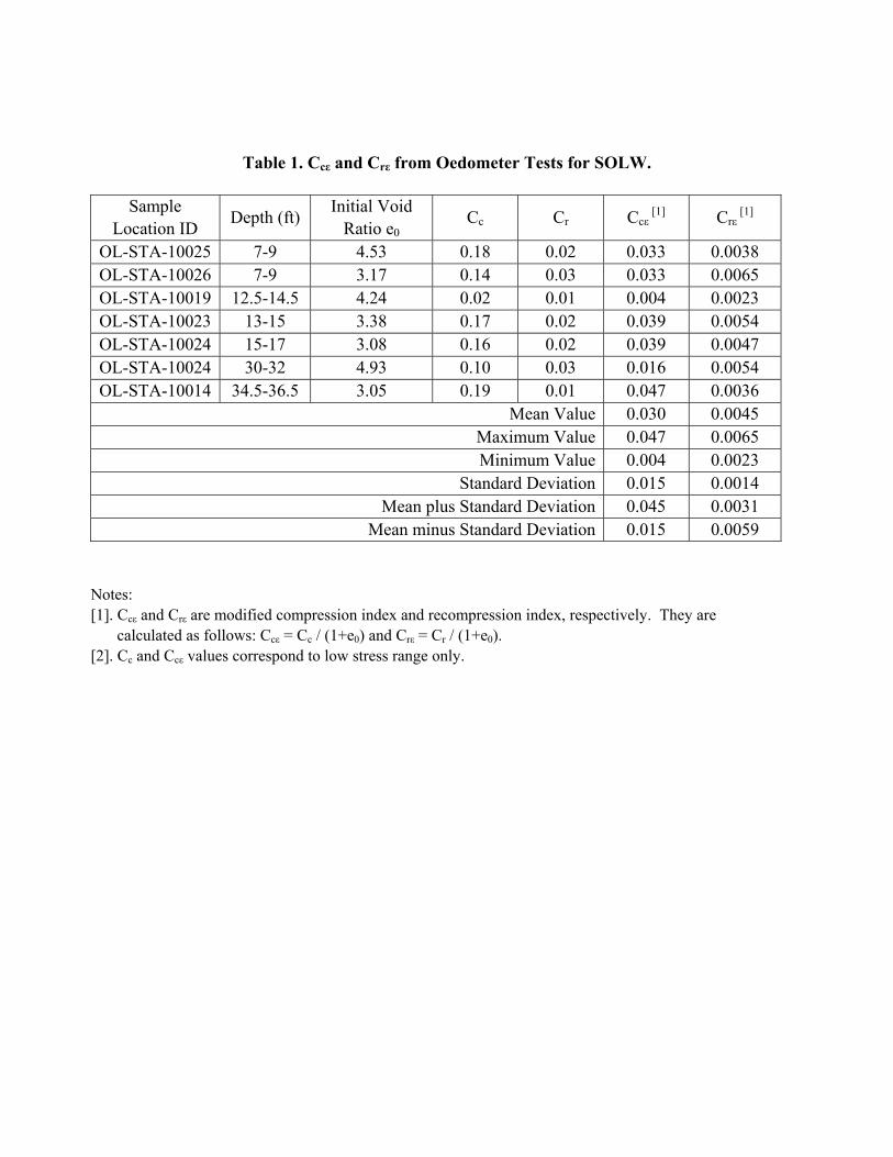
Table 1. Ccε and Crε from Oedometer Tests for SOLW.

Sample Location ID Depth (ft) Initial Void

Ratio e0 Cc Cr Ccε

[1] Crε [1]

OL-STA-10025 7-9 4.53 0.18 0.02 0.033 0.0038 OL-STA-10026 7-9 3.17 0.14 0.03 0.033 0.0065 OL-STA-10019 12.5-14.5 4.24 0.02 0.01 0.004 0.0023 OL-STA-10023 13-15 3.38 0.17 0.02 0.039 0.0054 OL-STA-10024 15-17 3.08 0.16 0.02 0.039 0.0047 OL-STA-10024 30-32 4.93 0.10 0.03 0.016 0.0054 OL-STA-10014 34.5-36.5 3.05 0.19 0.01 0.047 0.0036

Mean Value 0.030 0.0045 Maximum Value 0.047 0.0065 Minimum Value 0.004 0.0023

Standard Deviation 0.015 0.0014 Mean plus Standard Deviation 0.045 0.0031

Mean minus Standard Deviation 0.015 0.0059

Notes: [1]. Ccε and Crε are modified compression index and recompression index, respectively. They are

calculated as follows: Ccε = Cc / (1+e0) and Crε = Cr / (1+e0). [2]. Cc and Ccε values correspond to low stress range only.

Table 2. Ccε and Crε from Oedometer Tests for Marl.


Ratio e0 Cc Cr Ccε

[1] Crε [1]

OL-STA-20001 20-22 1.87 0.37 0.02 0.127 0.0082 OL-STA-20007 23-25 1.89 0.41 0.03 0.142 0.0113 OL-STA-20004 36.6-38.6 0.90 0.16 0.02 0.083 0.0103




Note: [1]. Ccε and Crε are modified compression index and recompression index, respectively. They are

calculated as follows: Ccε = Cc / (1+e0) and Crε = Cr / (1+e0).

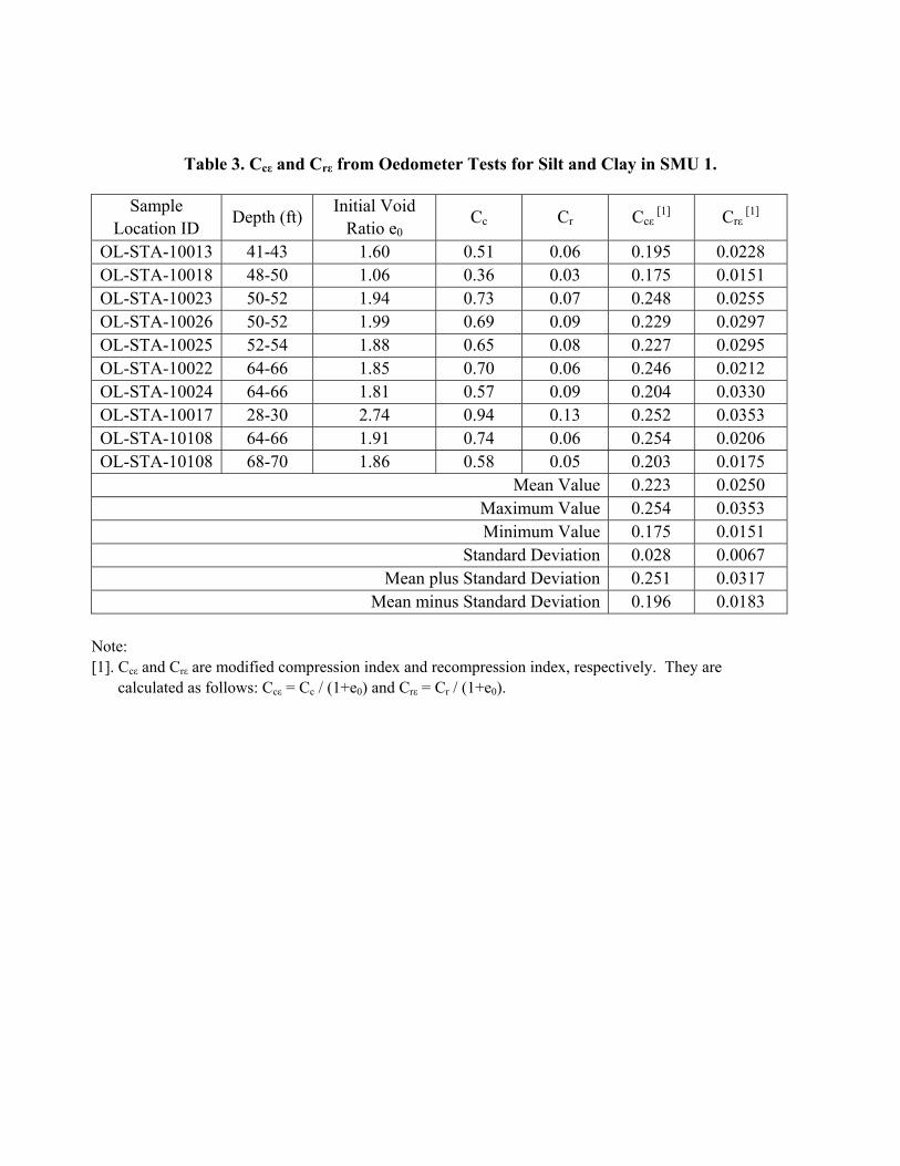
Table 3. Ccε and Crε from Oedometer Tests for Silt and Clay in SMU 1.


Ratio e0 Cc Cr Ccε

[1] Crε [1]

OL-STA-10013 41-43 1.60 0.51 0.06 0.195 0.0228 OL-STA-10018 48-50 1.06 0.36 0.03 0.175 0.0151 OL-STA-10023 50-52 1.94 0.73 0.07 0.248 0.0255 OL-STA-10026 50-52 1.99 0.69 0.09 0.229 0.0297 OL-STA-10025 52-54 1.88 0.65 0.08 0.227 0.0295 OL-STA-10022 64-66 1.85 0.70 0.06 0.246 0.0212 OL-STA-10024 64-66 1.81 0.57 0.09 0.204 0.0330 OL-STA-10017 28-30 2.74 0.94 0.13 0.252 0.0353 OL-STA-10108 64-66 1.91 0.74 0.06 0.254 0.0206 OL-STA-10108 68-70 1.86 0.58 0.05 0.203 0.0175






Table 4. Ccε and Crε from Oedometer Tests for Silt and Clay in SMU 2.


Ratio e0 Cc Cr Ccε

[1] Crε [1]

OL-STA-20007 38.6-40.6 1.33 0.49 0.05 0.210 0.0222 OL-STA-20001 44.9-46.9 0.95 0.26 0.04 0.134 0.0223 OL-STA-20018 47-49 0.91 0.23 0.02 0.119 0.0090






Table 5. Summary of the Material Properties used in Analysis.

Materials Unit

Weight (pcf)

Consolidation Parameters Hydraulic Conductivity

(cm/s) Ccε Crε Cαε cv (ft2/d)

Cap 120 N/A N/A N/A N/A N/A

SOLW 81 0.030[1] 0.0045 0.0011 3.500 1×10-5

Marl 98 0.117 0.0099 0.0050 0.090 (SMU 1) 0.100 (SMU 2)[2] 1×10-7

Silt and Clay (SMU 1) 108 0.223 0.0250 0.0100 0.090 1×10-7

Silt and Clay (SMU 2) 108 0.154 0.0179 0.0050 0.100 1×10-7

Notes: [1]. Ccε value corresponds to low stress range only. [2]. The interpreted cv of Marl is 0.135 ft2/d as presented in Figure 11. However, for the purpose of analysis, the cv of Marl was

assumed to be the same as Silt and Clay (i.e., 0.09 and 0.1 ft2/d in SMUs 1 and 2, respectively) in settlement calculations, as presented in Section 4.3.

Table 6. Selected Reasonable Upper and Lower Bound Values for Consolidation Parameters.

Material Ccε Crε Cαε cv (ft2/d)

Selected Reasonable Upper Bound Values SOLW 0.045 0.0059 0.0030 7.000

Marl 0.142 0.0110 0.0080 0.130 (SMU 1) 0.230 (SMU 2)[1]

Silt and Clay (SMU 1) 0.251 0.0317 0.0130 0.130 Silt and Clay (SMU 2) 0.203 0.0220 0.0070 0.230

Selected Reasonable Lower Bound Values SOLW 0.015 0.0031 0.0003 0.050[2] Marl 0.087 0.0083 0.0025 0.050[2]

Silt and Clay (SMU 1) 0.196 0.0183 0.0070 0.050 Silt and Clay (SMU 2) 0.119 0.0102 0.0040 0.050

Notes: [1]. The interpreted reasonable upper bound value of cv of Marl is 0.15 ft2/d, as presented in

Figure 11. However, for the purpose of analysis, the reasonable upper bound value of cv of Marl was assumed the same as Silt and Clay (i.e., 0.13 and 0.23 ft2/d in SMUs 1 and 2, respectively) in the settlement calculations, as presented in Section 4.3.

[2]. The interpreted reasonable lower bound values of cv of SOLW and Marl are 0.1 and 0.12 ft2/d, respectively, as presented in Figures 10 and 11. However, for the purpose of analysis, the reasonable lower bound values of cv of SOLW and Marl were assumed the same as Silt and Clay (i.e., 0.05 ft2/d) in the settlement calculations, as presented in Section 4.3.

FIGURES

Figure 1. Remediation Area D.

Remediation Area D

Notes: 1. Contours of the existing ground/lake bottom were provided by Parsons

and included the topographic survey in WB-B/HB issued by CNY Land Surveying in Baldwinsville, NY on 18 April, 2008.

2. Boundaries of SMUs and Remediation Area D were provided by Parsons.

SMU 8

SMU 1

SMU 7

SMU 2

WASTEBED B

HARBOR BROOK

Figure 2. Remediation Area D Preliminary Dredging Plan (Figure provided by Parsons to Geosyntec).

N

Figure 3. Cap Thickness in Remediation Area D (Figure provided to Geosyntec by Parsons).

Note: The above cap configuration was assumed for the purposes of the analyses presented herein. Slight modifications to cap thickness should not impact the outcome of the analyses. As necessary, changes to the cap configuration will be addressed in subsequent design submittals.

Figure 4. Areas and Subsurface Layer Thicknesses.

SOLW Marl Silt and Clay1 30 25 1002 20 5 903 20 10 504 45 10 605 50 5 606 45 20 307 45 0 308 20 15 309 35 10 6010 20 10 2011 30 10 2012 20 10 30

AreaSelected Subsurface Layer Thickness (ft)

WASTEBED B

HARBOR BROOK

SMU 7

SMU 8

SMU 2

SMU 1

1

3

5

7

9

11

13

15

1 10 100 1000 10000 100000

Void Ratio

Vertical Effective Stress (psf)

OL‐STA‐10024 (30‐32 ft)

OL‐STA‐10024 (15‐17 ft)

OL‐STA‐10023 (13‐15 ft)

OL‐STA‐10026 (7‐9 ft)

OL‐STA‐10025 (7‐9 ft)

OL‐STA‐10019 (12.5‐14.5 ft)

OL‐STA‐10014 (34.5‐36.5 ft)

OL‐VC‐10037 (9.9‐13.2 ft)

OL‐VC‐10038 (9.9‐13.2 ft)

OL‐VC‐10062A (3.3‐6.6 ft)

OL‐VC‐10080 (9.9‐13.2 ft)

OL‐VC‐10081A (13.2‐16.5 ft)

OL‐VC‐10105 (0‐3.3 ft)

OL‐STA‐10108 (47‐49 ft)

OL‐STA‐10022‐VC (9.9‐13.2 ft)

OL‐STA‐10016‐VC (0‐3.3 ft)

OL‐STA‐10026‐VC (3.3‐6.6 ft)

OL‐STA‐10018‐VC (6.6‐9.9 ft)

OL‐STA‐10015‐VC (9.9‐13.2 ft)

OL‐STA‐10017‐VC (0‐3.3 ft)

OL‐STA‐10017‐VC (9.9‐12.6 ft)

OL‐STA‐10024‐VC (6.6‐9.9 ft)

Figure 5. Comparison of Results from Conventional Oedometer Tests and SIC Tests.

Stress range of interest for SOLW settlement calculations

Range of “apparent” preconsolidation

Dashed Lines: SIC Tests

Solid Lines: Oedometer Tests

Cr

Cc (low stress)

Cc (high stress)

0.000

0.002

0.004

0.006

0.008

0.010

0.012

0.014

0.016

0.001 0.01 0.1 1 10

Mod

ified

Sec

onda

ry C

ompr

essi

on In

dex

Stress Ratio σv'/σp'

Modified Secondary Compression Index of SOLW

OL-STA-10024 (30-32ft)OL-STA-10014 (34.5-36.5ft)OL-STA-10024 (15-17ft)OL-STA-10023 (13-15ft)OL-STA-10025 (7-9ft)OL-STA-10026 (7-9ft)OL-STA-10019 (12.5-14.5ft)Representative ValueReasonable Lower Bound ValueReasonable Upper Bound Value

0.0011

0.0003

0.003

Figure 6. Interpretation of Modified Secondary Compression Index for SOLW.

Note: The ratio of σv'/σp' of SOLW in the field before and after capping was estimated to be between 0.1 and 1 according to the assumed subsurface layer thicknesses.

0.000

0.002

0.004

0.006

0.008

0.010

0.012

0.014

0.016

0.018

0.020

0.001 0.01 0.1 1 10

Mod

ified

Sec

onda

ry C

ompr

essi

on In

dex


Modified Secondary Compression Index of Marl

OL-STA-20007 (23-25ft)

OL-STA-20004 (36.6-38.6ft)

OL-STA-20001 (20-22ft)

Representative Value

Reasonable Lower Bound Value

Reasonable Upper Bound Value

0.008

0.005

0.0025

Figure 7. Interpretation of Modified Secondary Compression Index for Marl.

Note: The ratio of σv'/σp' of Marl in the field before and after capping was estimated to be between 0.7 and 3 according to the assumed subsurface layer thicknesses.

0.000

0.002

0.004

0.006

0.008

0.010

0.012

0.014

0.016

0.018

0.020

0.001 0.01 0.1 1 10

Mod

ified

Sec

onda

ry C

ompr

essi

on In

dex


Modified Secondary Compression Index of Silt and Clay in SMU 1

OL-STA-10023 (50-52ft)OL-STA-10022 (64-66ft)OL-STA-10018 (48-50ft)OL-STA-10025 (52-54ft)OL-STA-10024 (64-66ft)OL-STA-10013 (41-43ft)OL-STA-10026 (50-52ft)OL-STA-10017 (28-30ft)10108 (64-66ft)10108 (68-70ft)Representative ValueReasonable Lower Bound ValueReasonable Upper Bound Value

0.013

0.007

0.01

Figure 8. Interpretation of Modified Secondary Compression Index for Silt and Clay in SMU 1.

Note: The ratio of σv'/σp' of Silt and Clay in the field before and after capping was estimated to be between 0.9 and 3 according to the assumed subsurface layer thicknesses.

0.000

0.002

0.004

0.006

0.008

0.010

0.012

0.014

0.016

0.018

0.020

0.001 0.01 0.1 1 10

Mod

ified

Sec

onda

ry C

ompr

essi

on In

dex


Modified Secondary Compression Index of Silt and Clay in SMU 2

OL-STA-20018 (47-49ft)OL-STA-20001 (44.9-46.9ft)OL-STA-20007 (38.6-40.6ft)Representative ValueReasonable Lower Bound ValueReasonable Upper Bound Value

0.007

0.005

0.004

Figure 9. Interpretation of Modified Secondary Compression Index for Silt and Clay in SMU 2. Note: The ratio of σv'/σp' of Silt and Clay in the field before and after capping was estimated to be between 0.9 and 3 according to the assumed subsurface layer thicknesses.

0.00

1.00

2.00

3.00

4.00

5.00

6.00

7.00

8.00

9.00

10.00

0.001 0.01 0.1 1

Coe

ffici

ent o

f Con

solid

atio

n c v

(ft2 /d

)


Coefficient of Consolidation of SOLW

OL-STA-10024 30-32ftOL-STA-10024 15-17ftOL-STA-10026 7-9ftOL-STA-10025 7-9ftOL-STA-10019 7-9ftOL-STA-10023 13-15ftOL-STA-10014 34.5-36.5ftRepresentative ValueReasonable Lower Bound ValueReasonable Upper Bound Value

7.0

3.5

0.1

Figure 10. Interpretation of Coefficient of Consolidation Index for SOLW. Note: The ratio of σv'/σp' of SOLW in the field before and after capping was estimated to be between 0.1 and 1 according to the assumed subsurface layer thicknesses.

0.00

0.05

0.10

0.15

0.20

0.25

0.30

0.35

0.40

0.001 0.01 0.1 1

Coe

ffici

ent o

f Con

solid

atio

n c v

(ft2 /d

)


Coefficient of Consolidation of Marl

OL-STA-20001 (20-22ft)

OL-STA-20007 (23-25ft)

OL-STA-20004 (36.6-38.6ft)



Reasonable Upper Bound Value

0.15

0.1350.12

Figure 11. Interpretation of Coefficient of Consolidation Index for Marl.

Note: The ratio of σv'/σp' of Marl in the field before and after capping was estimated to be between 0.7 and 3 according to the assumed subsurface layer thicknesses.

0.00

0.10

0.20

0.30

0.40

0.50

0.60

0.70

0.80

0.001 0.01 0.1 1

Coe

ffici

ent o

f Con

solid

atio

n c v

(ft2 /d

)


Coefficient of Consolidation of Silt and Clay in SMU 1

OL-STA-10023 (50-52ft)OL-STA-10022 (64-66ft)OL-STA-10026 (50-52ft)OL-STA-10025 (52-54ft)OL-STA-10024 (64-66ft)OL-STA-10017 (28-30ft)OL-STA-10018 (48-50ft)OL-STA-10013 (41-43ft)OL-STA-10108 (64-66ft)OL-STA-10108 (68-70ft)Representative ValueReasonable Lower Bound ValueReasonable Upper Bound Value 0.13

0.09

0.05

Figure 12. Interpretation of Coefficient of Consolidation Index for Silt and Clay in SMU 1. Note: The ratio of σv'/σp' of Silt and Clay in the field before and after capping was estimated to be between 0.9 and 3 according to the assumed subsurface layer thicknesses.

0.00

0.10

0.20

0.30

0.40

0.50

0.001 0.01 0.1 1

Coe

ffic

ient

of C

onso

lidat

ion

c v(f

t2/d

)


Coefficient of Consolidation of Silt and Clay in SMU 2

OL-STA-20018 (47-49ft)

OL-STA-20001 (44.9-46.9ft)

OL-STA-20007 (38.6-40.6ft)



Reasonable Upper Bound Value0.23

0.1

0.05

Figure 13. Interpretation of Coefficient of Consolidation Index for Silt and Clay in SMU 2. Note: The ratio of σv'/σp' of Silt and Clay in field before and after capping was estimated to be between 0.9 and 3 according to the assumed subsurface layer thicknesses.

(a)

(b)

Figure 14. Finite difference method based numerical solution for the 1-D consolidation equation: (a) for nodes within homogeneous layers; and (b) for

interface node between 2 layers. Note that the consolidation water flow direction is vertical. (source: Das, 2008)

0.0

0.4

0.8

1.2

1.6

2.0

0 2 4 6 8 10

Estim

ated

Set

tlem

ent a

t Top

of C

ap (f

t)

Dredge Depth (ft)

Area 1

Cap Thickness = 3 ft


Cap Thickness = 5.5 ft

(SOLW 30', Marl 25', Silt/Clay 100')

0.0

0.4

0.8

1.2

1.6

2.0

0 2 4 6 8 10

Estim

ated

Set

tlem

ent a

t Top

of C

ap (f

t)

Dredge Depth (ft)

Area 2





0.0

0.4

0.8

1.2

1.6

2.0

0 2 4 6 8 10

Estim

ated

Set

tlem

ent a

t Top

of C

ap (f

t)

Dredge Depth (ft)

Area 3





0.0

0.4

0.8

1.2

1.6

2.0

0 2 4 6 8 10

Estim

ated

Set

tlem

ent a

t Top

of C

ap (f

t)

Dredge Depth (ft)

Area 4





Figure 15. Settlement Analysis Results for Areas 1 to 12 for 30-Year Period.

0.0

0.4

0.8

1.2

1.6

2.0

0 2 4 6 8 10

Estim

ated

Set

tlem

ent a

t Top

of C

ap (f

t)

Dredge Depth (ft)

Area 5





0.0

0.4

0.8

1.2

1.6

2.0

0 2 4 6 8 10

Estim

ated

Set

tlem

ent a

t Top

of C

ap (f

t)

Dredge Depth (ft)

Area 6





0.0

0.4

0.8

1.2

1.6

2.0

0 2 4 6 8 10

Estim

ated

Set

tlem

ent a

t Top

of C

ap (f

t)

Dredge Depth (ft)

Area 7





0.0

0.4

0.8

1.2

1.6

2.0

0 2 4 6 8 10

Estim

ated

Set

tlem

ent a

t Top

of C

ap (f

t)

Dredge Depth (ft)

Area 8





Figure 15. Settlement Analysis Results for Areas 1 to 12 for 30-Year Period (continued).

0.0

0.4

0.8

1.2

1.6

2.0

0 2 4 6 8 10

Estim

ated

Set

tlem

ent a

t Top

of C

ap (f

t)

Dredge Depth (ft)

Area 9





0.0

0.4

0.8

1.2

1.6

2.0

0 2 4 6 8 10

Estim

ated

Set

tlem

ent a

t Top

of C

ap (f

t)

Dredge Depth (ft)

Area 10





0.0

0.4

0.8

1.2

1.6

2.0

0 2 4 6 8 10Estim

ated

Set

tlem

ent a

t Top

of C

ap (f

t)

Dredge Depth (ft)

Area 11




SOLW 30', Marl 10', Silt/Clay 20'

0.0

0.4

0.8

1.2

1.6

2.0

0 2 4 6 8 10

Estim

ated

Set

tlem

ent a

t Top

of C

ap (f

t)

Dredge Depth (ft)

Area 12





Figure 15. Settlement Analysis Results for Areas 1 to 12 for 30-Year Period (continued).

0.0

0.2

0.4

0.6

0.8

1.0

0 2 4 6 8 10

Estim

ated

Set

tlem

ent a

t Top

of C

ap (f

t)

Dredge Depth (ft)

Area 3





Figure 16. Settlement Analysis Results for Area 3 for 2-Year Period.

0.00

0.05

0.10

0.15

0.20

0.25

0.30

0.35

0.40

0.45

0.50

0 2 4 6 8 10 12 14 16 18 20 22 24 26 28 30

Cum

ulat

ive

Upw

ard

Con

solid

atio

n W

ater

Fl

ow (f

t)

Time (years)

Area 1

Area 7

Area 7 - Best Fit Curve

y=0.211x0.235

Figure 17. Calculated Cumulative Consolidation Water Flow.

Note: Calculations were performed for 2 m dredge and 4 ft thick cap.

ATTACHMENT A

SUBSURFACE LAYER THICKNESS CONTOURS

Figure A1. The Thickness of SOLW in Remediation Area D

Note: 1. The subsurface thickness contours were developed based on the elevations of each layer from the boring logs provided by Parsons, as presented in Section 2. 2. The subsurface thickness in the area that is not covered by the contours presented in this figure was estimated based on boring logs provided by Parsons.

Figure A2. The Thickness of Marl in Remediation Area D

Note: 1. The subsurface thickness contours were developed based on the elevations of each layer from the boring logs provided by Parsons, as presented in Section 2. 2. The subsurface thickness in the area that is not covered by the contours presented in this figure was estimated based on boring logs provided by Parsons.

Figure A3. The Thickness of Silt and Clay in Remediation Area D

Note: 1. The subsurface thickness contours were developed based on the elevations of each layer from the boring logs provided by Parsons. The bottom of Silt and Clay was below the depth of the shallow borings and was

developed based on a limited number of borings that went to deeper depths in the ILWD, as presented in Section 2. 2. The subsurface thickness in the area that is not covered by the contours presented in this figure was estimated based on boring logs provided by Parsons.

ATTACHMENT B

CONVENTIONAL OEDOMETER TEST RESULTS SUMMARY

Summary of Consolidation Test Data – Phase I PDI Field Depth Average Compression Recompression Initial Void Initial Water Preconsolidation

Location ID Sample ID Depth Index Index Ratio Content Pressure(ft) (ft) (Cc) (Cr) (eo) (%) (tsf)

OL-STA-10013 OL-0110-05 41-43 42 0.51 0.06 1.60 57.6 0.6OL-STA-10014 OL-0110-08 34.5-36.5 35.5 0.94 0.01 3.05 113.1 0.6OL-STA-10017 OL-0110-20 28-30 29 0.94 0.13 2.74 103.7 0.3OL-STA-10018 OL-0110-27 48-50 49 0.36 0.03 1.06 36.5 0.7OL-STA-10019 OL-0110-30 12.5-14.5 13.5 0.08 0.01 4.24 148.7 1.0OL-STA-10022 OL-0110-49 64-66 65 0.70 0.06 1.85 67.2 0.8OL-STA-10023 OL-0052-06 13-15 14 1.59 0.02 3.38 142.2 0.5OL-STA-10023 OL-0052-04 50-52 51 0.73 0.07 1.94 72.5 0.9OL-STA-10024 OL-0052-07 15-17 16 1.18 0.02 3.08 120.9 0.8OL-STA-10024 OL-0052-09 30-32 31 2.84 0.03 4.93 180.0 1.4OL-STA-10024 OL-0052-12 64-66 65 0.57 0.09 1.81 63.4 0.6OL-STA-10025 OL-0052-13 7-9 8 2.04 0.02 4.53 183.6 0.9OL-STA-10025 OL-0052-16 52-54 53 0.65 0.08 1.88 70.3 0.7OL-STA-10026 OL-0052-19 7-9 8 1.22 0.03 3.17 105.7 0.9OL-STA-10026 OL-0052-22 50-52 51 0.69 0.09 1.99 76.5 0.7OL-STA-20001 OL-0072-07 20-22 21 0.37 0.02 1.87 64.2 0.3OL-STA-20001 OL-0072-09 44.9-46.9 45.9 0.26 0.04 0.95 32.7 0.5OL-STA-20004 OL-0072-01 12-14 13 0.72 0.01 2.91 102.3 0.3OL-STA-20004 OL-0072-02 36.6-38.6 37.6 0.16 0.02 0.90 31.4 0.4OL-STA-20007 OL-0072-04 23-25 24 0.41 0.03 1.89 65.8 0.3OL-STA-20007 OL-0072-05 38.6-40.6 39.6 0.49 0.05 1.33 48.6 0.5OL-STA-20016 OL-0110-52 27-29 28 0.19 0.04 0.89 30.9 0.4OL-STA-20017 OL-0110-57 10-12 11 0.51 0.01 1.42 37.2 0.4OL-STA-20017 OL-0110-59 42-44 43 0.22 0.03 0.87 31.1 0.6OL-STA-20018 OL-0110-55 47-49 48 0.23 0.02 0.91 32.7 0.7

Summary of Consolidation Test Data – Phase II PDI

Modified ModifiedField Depth Average Compression Recompression Compression Recompression Initial Void Initial Water Preconsolidation

Location ID Sample ID Depth Index Index Index Index Ratio Content Pressure(ft) (ft) (Cc) (Cr) (Ccε) (Crε) (eo) (%) (psf)

OL-STA-10108 OL-0267-01 64-66 65 0.74 0.06 0.25 0.02 1.91 70.8 1702OL-STA-10108 OL-0267-02 68-70 69 0.58 0.05 0.20 0.02 1.86 65.3 1032 (disturbed sample)

Notes: 1. The Cc values of SOLW in this table correspond to high stress (i.e., >1000 psf) range and were not used in analysis. 2. The modified compression index Ccε and recompression index Crε are calculated as follows: Ccε = Cc / (1+e0) and Crε = Cr / (1+e0). 3. These summary tables were provided to Geosyntec by Parsons.

ATTACHMENT C

EXAMPLES OF CALCULATIONS

(For Area 7 with 2 m dredge and 4 ft thick cap)

An Example of Settlement Calculations

Input:Dredging Depth 6.6 ft

30 years

Soil LayersThickness

(ft)Unit Weight

(pcf) OCR Ccε Crε CαCoef. of Con. cv

(ft2/d)Time of 90%

primary con. (y)t2/t1 for

Secondary Con.# of

SublayersCap 4 120SOLW 45 81 1 0.030 0.0045 0.0011 3.500 1.3 22.3 18Marl 0 98 1 0.117 0.0099 0.0050 0.090 5.8 5.2 0Silt/Clay 30 108 1 0.223 0.0250 0.0100 0.090 5.8 5.2 6Water 62.4

Consider Total Settlement in

Calculated Settlement (ft):

Primary Settlement

Secondary Settlement

Total Settlement

SOLW 0.158 0.057 0.215Marl 0.000 0.000 0.000Silt/Clay 0.242 0.215 0.457Total 0.40 0.27 0.67

Calculation for SOLWLayer No. 1Layer Thickness, m / ft 2.1333333Midpoint Depth from Dredge Bot, m/ft 1.0666667Effective Stress Before Dredging, KPa/psf 142.6Initial Effective Stress, KPa/psf 19.84Final Effective Stress, KPa/psf 250.24OCR 1Preconsolidation Pressure, KPa/psf 142.6Modified Primary Compression Index, Ccε 0.03Modified Recompression Index, Crε 0.0045Modified Secondary Compression Index, Cαε 0.0011ratio of t2 / t1 22.3SettlementsPrimary Settlement, (m / ft) 0.024Secondary Settlement (m / ft) 0.003Total Settlement (m / ft) 0.027

Layer No. 2Layer Thickness, m / ft 2.1333333Midpoint Depth from Dredge Bot, m/ft 3.2Effective Stress Before Dredging, KPa/psf 182.28Initial Effective Stress, KPa/psf 59.52Final Effective Stress, KPa/psf 289.92OCR 1Preconsolidation Pressure, KPa/psf 182.28Modified Primary Compression Index, Ccε 0.03Modified Recompression Index, Crε 0.0045Modified Secondary Compression Index, Cαε 0.0011ratio of t2 / t1 22.3SettlementsPrimary Settlement, (m / ft) 0.018Secondary Settlement (m / ft) 0.003Total Settlement (m / ft) 0.021




Layer No. 6Layer Thickness, m / ft 2.1333333Midpoint Depth from Dredge Bot, m/ft 11.733333Effective Stress Before Dredging, KPa/psf 341Initial Effective Stress, KPa/psf 218.24Final Effective Stress, KPa/psf 448.64OCR 1Preconsolidation Pressure, KPa/psf 341Modified Primary Compression Index, Ccε 0.03Modified Recompression Index, Crε 0.0045Modified Secondary Compression Index, Cαε 0.0011ratio of t2 / t1 22.3SettlementsPrimary Settlement, (m / ft) 0.009Secondary Settlement (m / ft) 0.003Total Settlement (m / ft) 0.013


Layer No. 8Layer Thickness, m / ft 2.1333333Midpoint Depth from Dredge Bot, m/ft 16Effective Stress Before Dredging, KPa/psf 420.36Initial Effective Stress, KPa/psf 297.6Final Effective Stress, KPa/psf 528OCR 1Preconsolidation Pressure, KPa/psf 420.36Modified Primary Compression Index, Ccε 0.03Modified Recompression Index, Crε 0.0045Modified Secondary Compression Index, Cαε 0.0011ratio of t2 / t1 22.3SettlementsPrimary Settlement, (m / ft) 0.008Secondary Settlement (m / ft) 0.003Total Settlement (m / ft) 0.011





Layer No. 13Layer Thickness, m / ft 2.1333333Midpoint Depth from Dredge Bot, m/ft 26.666667Effective Stress Before Dredging, KPa/psf 618.76Initial Effective Stress, KPa/psf 496Final Effective Stress, KPa/psf 726.4OCR 1Preconsolidation Pressure, KPa/psf 618.76Modified Primary Compression Index, Ccε 0.03Modified Recompression Index, Crε 0.0045Modified Secondary Compression Index, Cαε 0.0011ratio of t2 / t1 22.3SettlementsPrimary Settlement, (m / ft) 0.005Secondary Settlement (m / ft) 0.003Total Settlement (m / ft) 0.009






Calculation for Silt and ClayLayer No. 1Layer Thickness, m / ft 5Midpoint Depth from Top of Silt/Clay, m/ft 2.5Effective Stress Before Dredging, KPa/psf 951Initial Effective Stress, KPa/psf 828.24Final Effective Stress, KPa/psf 1058.64OCR 1Preconsolidation Pressure, KPa/psf 951Modified Primary Compression Index, Ccε 0.223Modified Recompression Index, Crε 0.025Modified Secondary Compression Index, Cαε 0.01ratio of t2 / t1 5.2SettlementsPrimary Settlement, (m / ft) 0.059Secondary Settlement (m / ft) 0.036Total Settlement (m / ft) 0.095

Layer No. 2Layer Thickness, m / ft 5Midpoint Depth from Top of Silt/Clay, m/ft 7.5Effective Stress Before Dredging, KPa/psf 1179Initial Effective Stress, KPa/psf 1056.24Final Effective Stress, KPa/psf 1286.64OCR 1Preconsolidation Pressure, KPa/psf 1179Modified Primary Compression Index, Ccε 0.223Modified Recompression Index, Crε 0.025Modified Secondary Compression Index, Cαε 0.01ratio of t2 / t1 5.2SettlementsPrimary Settlement, (m / ft) 0.048Secondary Settlement (m / ft) 0.036Total Settlement (m / ft) 0.084





An Example Calculation of Upward Cumulative Consolidation Water Flow

LoadingCap thickness = 4 ft

Cap unit weight = 120 psfLoad = 230.4 psf

PropertiesTop Layer Bottom Layer

Type SOLW Silt and Clayk = 1.0E‐05 1.0E‐07 cm/s A = 0.7272

1.8E‐01 1.8E‐03 ft/d B = 2.0E+00Cv = 3.50 0.09 ft2/d C = 2.0E‐02H = 39 30 ft

Cαε = 0.0011 0.0100t90 = 435 2500 days

1.2 6.8 years

Reference ValueszR = 69.0 69.0 ftuR = 2.30 2.30 psftR = 1360 52900 days

4 145 yearsTime Step

Select δt to ensure convergence of solutionδt = 0.0030 0.0030 years

1 1 daysδt‐bar = 8.05E‐04 2.07E‐05

δz = 3 3 ftδz‐bar = 0.04 0.04

bar δt1/(δz)2 = 0.43 0.01 should be less than 0.5

U‐bar valuest (years) 0.00 0.00 0.01 0.01 0.01 0.02 0.02 0.02 0.02 0.03 0.03 0.03 0.04 0.04 0.04 0.05 0.05t (days) 0 1 2 3 4 5 7 8 9 10 11 12 13 14 15 16 18t‐bar 0.00 0.00 0.00 0.00 0.00 0.00 0.00 0.01 0.01 0.01 0.01 0.01 0.01 0.01 0.01 0.01 0.01

Z (ft) z‐bar s1 s2 s3 s4 s5 s6 s7 s8 s9 s10 s10 s10 s10 s10 s10 s10 s100 0.0 0 0 0 0 0 0 0 0 0 0 0 0 0 0 0 0 03 0.0 100 57 51 42 39 35 33 30 29 27 26 25 24 23 22 22 216 0.1 100 100 82 76 69 65 60 57 54 52 49 48 46 44 43 42 419 0.1 100 100 100 92 89 84 80 77 74 71 68 66 64 62 61 59 58

12 0.2 100 100 100 100 97 95 92 89 87 84 82 80 78 76 75 73 7115 0.2 100 100 100 100 100 99 98 96 94 93 91 89 88 86 85 83 8218 0.3 100 100 100 100 100 100 99 99 98 97 96 95 94 93 92 90 8921 0.3 100 100 100 100 100 100 100 100 99 99 99 98 97 96 96 95 9424 0.3 100 100 100 100 100 100 100 100 100 100 100 99 99 98 98 98 9727 0.4 100 100 100 100 100 100 100 100 100 100 100 100 100 99 99 99 9930 0.4 100 100 100 100 100 100 100 100 100 100 100 100 100 100 100 100 9933 0.5 100 100 100 100 100 100 100 100 100 100 100 100 100 100 100 100 10036 0.5 100 100 100 100 100 100 100 100 100 100 100 100 100 100 100 100 10039 0.6 100 100 100 100 100 100 100 100 100 100 100 100 100 100 100 100 10042 0.6 100 100 100 100 100 100 100 100 100 100 100 100 100 100 100 100 10045 0.7 100 100 100 100 100 100 100 100 100 100 100 100 100 100 100 100 10048 0.7 100 100 100 100 100 100 100 100 100 100 100 100 100 100 100 100 10051 0.7 100 100 100 100 100 100 100 100 100 100 100 100 100 100 100 100 10054 0.8 100 100 100 100 100 100 100 100 100 100 100 100 100 100 100 100 10057 0.8 100 100 100 100 100 100 100 100 100 100 100 100 100 100 100 100 10060 0.9 100 100 100 100 100 100 100 100 100 100 100 100 100 100 100 100 10063 0.9 100 100 100 100 100 100 100 100 100 100 100 99 99 99 99 99 9966 1.0 100 99 98 97 96 95 94 93 92 91 90 89 88 87 87 86 8569 1.0 0 0 0 0 0 0 0 0 0 0 0 0 0 0 0 0 0

Top LayerInitial Area = 3900 3900 3900 3900 3900 3900 3900 3900 3900 3900 3900 3900 3900 3900 3900 3900 3900

Current Area = 3700 3530 3468 3392 3342 3288 3244 3201 3162 3124 3090 3056 3024 2993 2963 2935 2907U‐ave= 5% 9% 11% 13% 14% 16% 17% 18% 19% 20% 21% 22% 22% 23% 24% 25% 25%

Final primary settlement (ft) = 0.16 0.16 0.16 0.16 0.16 0.16 0.16 0.16 0.16 0.16 0.16 0.16 0.16 0.16 0.16 0.16 0.16Current primary settlement (ft) = 0.01 0.02 0.02 0.02 0.02 0.02 0.03 0.03 0.03 0.03 0.03 0.03 0.04 0.04 0.04 0.04 0.04

Current secondary settlement (ft) = 0.00 0.00 0.00 0.00 0.00 0.00 0.00 0.00 0.00 0.00 0.00 0.00 0.00 0.00 0.00 0.00 0.00Current total settlement (ft) = 0.01 0.02 0.02 0.02 0.02 0.02 0.03 0.03 0.03 0.03 0.03 0.03 0.04 0.04 0.04 0.04 0.04

Bottom LayerInitial Area = 3000 3000 3000 3000 3000 3000 3000 3000 3000 3000 3000 3000 3000 3000 3000 3000 3000

Current Area = 2900 2896 2891 2887 2883 2879 2875 2871 2867 2863 2859 2855 2852 2848 2845 2841 2837U‐ave= 3% 3% 4% 4% 4% 4% 4% 4% 4% 5% 5% 5% 5% 5% 5% 5% 5%

Final primary settlement (ft) = 0.15 0.15 0.15 0.15 0.15 0.15 0.15 0.15 0.15 0.15 0.15 0.15 0.15 0.15 0.15 0.15 0.15Current primary settlement (ft) = 0.00 0.01 0.01 0.01 0.01 0.01 0.01 0.01 0.01 0.01 0.01 0.01 0.01 0.01 0.01 0.01 0.01

Current secondary settlement (ft) = 0.00 0.00 0.00 0.00 0.00 0.00 0.00 0.00 0.00 0.00 0.00 0.00 0.00 0.00 0.00 0.00 0.00Current total settlement (ft) = 0.00 0.01 0.01 0.01 0.01 0.01 0.01 0.01 0.01 0.01 0.01 0.01 0.01 0.01 0.01 0.01 0.01

Total Total current settlement (ft) = 0.01 0.02 0.02 0.03 0.03 0.03 0.03 0.03 0.04 0.04 0.04 0.04 0.04 0.04 0.05 0.05 0.05

Note: Due to the limited paper size, only part of the calculation sheet is shown here.

U bar and settlement results summaryUave top 5% 16% 30% 51% 73% 93% 99% 100% 100% 100%Uave bot 3% 4% 6% 12% 22% 41% 79% 98% 100% 100%t (years) 0.00 0.02 0.07 0.23 0.54 1.29 4.21 10.54 18.97 30.00t (days) 0.00 5.48 25.19 82.13 196.01 469.75 1536.29 3845.64 6924.78 10950.00Z (ft) t = 0, Ut=5%, Ub=t = 5 days, Ut=16%, Ub t = 25 days, Ut=30%, Ub=6t = 82 days, Ut= t = 196 days, Ut = 1.3 years, Utt = 4.2 years, Utt = 10.5 years, Ut = 19.0 years, Ut = 30 years, Ut=100%, Ub=100%

0 0 0 0 0 0 0 0 0 0 03 100 35 18 10 5 1 0 0 0 06 100 65 34 20 10 3 0 0 0 09 100 84 50 29 15 4 0 0 0 0

12 100 95 63 38 20 5 1 0 0 015 100 99 74 46 25 7 1 0 0 018 100 100 82 54 29 8 1 0 0 021 100 100 88 60 33 9 1 0 0 024 100 100 93 66 36 10 1 0 0 027 100 100 96 71 39 11 1 0 0 030 100 100 98 75 41 12 1 0 0 033 100 100 99 78 43 12 1 0 0 036 100 100 99 80 45 13 1 0 0 039 100 100 100 81 45 13 2 0 0 042 100 100 100 96 77 43 12 1 0 045 100 100 100 99 92 66 20 2 0 048 100 100 100 100 98 79 27 3 0 051 100 100 100 100 99 86 32 3 0 054 100 100 100 100 98 85 33 4 0 057 100 100 100 99 95 79 31 3 0 060 100 100 100 97 86 67 26 3 0 063 100 100 98 87 69 48 19 2 0 066 100 95 80 57 39 26 10 1 0 069 0 0 0 0 0 0 0 0 0 0

Cumulative Upward Conso 0.01 0.03 0.06 0.10 0.15 0.21 0.30 0.37 0.42 0.46

ATTACHMENT D

CALCULATED EXCESS PORE WATER PRESSURE ISOCHRONES

Note: In the charts presented herein, Ut = the average degree of consolidation of top layer (i.e., SOLW); Ub = the average degree of consolidation of bottom layer (i.e., Marl + Silt and Clay).

0

20

40

60

80

100

120

140

0 20 40 60 80 100

Deo

th (ft)

Relative Excess Pore Pressure (%)

Area 1 (6.6' dredge, 4' cap)

t = 0, Ut=3%, Ub=1%

t = 5 days, Ut=21%, Ub=1%

t = 27 days, Ut=45%, Ub=2%

t = 70 days, Ut=70%, Ub=3%

t = 240 days, Ut=96%, Ub=7%

t = 2.1 years, Ut=99%, Ub=14%

t = 7.4 years, Ut=100%, Ub=28%

t = 13.7 years, Ut=100%, Ub=38%

t = 17.9 years, Ut=100%, Ub=43%

t = 30 years, Ut=100%, Ub=56%

0

10

20

30

40

50

60

0 20 40 60 80 100

Dep

th (ft)

Relative Excess Pore Pressure (%)

Area 7 (6.6' dredge, 4' cap)

t = 0, Ut=5%, Ub=3%

t = 5 days, Ut=16%, Ub=4%

t = 25 days, Ut=30%, Ub=6%

t = 82 days, Ut=51%, Ub=12%

t = 196 days, Ut=73%, Ub=22%

t = 1.3 years, Ut=93%, Ub=41%

t = 4.2 years, Ut=99%, Ub=79%

t = 10.5 years, Ut=100%, Ub=98%

t = 19.0 years, Ut=100%, Ub=100%

t = 30 years, Ut=100%, Ub=100%

Documents

E.2 CAP-INDUCED SETTLEMENT EVALUATION FOR …