E0YLEVEL,

•--

TN no. N-1590

title: SHOCK SPECTRUM CALCULATION FROM

ACCELERATION TIME HISTORIES DTICELECTE

author: H. A. Gaberson MAR 3 1 1981

date: September 1980 B

sponsor: Naval Facilities Engineeri:ng Conmand S

program nos: YF53.534.006.0l.017

_ _ _ CIVIL ENGINEERING LABORATORYNAVAL CONSTRUCTION BATTALION CENTERPort Hueneme, California 93043Approved for public release; distribuLion unlimited.

U 2 .31 027

UnclassifiedSECURITY CLASSIFICATIONe OF THIS PAGE (Uh-e DOg~ 9--t)____________________

REPORT DOCUMENTATION PAGE BEFORE COMPLETING FORMI. REPRT NU9911ACCUIISIO6 NO .3ASCCSPICHT'S CATALOG NUM06ft

TN-i1590 DO46tý7J&

JPCK;fECRU fALCULATION FROM Jul _____________1978

L4 -ACELEPLATIONJINME gJISTORIES,0 J V OCR eOOIN aOR, P19POiT NUMOCR

CIVIL ENGINEERING LABORATORY AI OKU~ USR

Naval Construction Battalion Center

Naval Facilities Engineering CommandAlexandria, Virgini3 22332 6

14. MONITORING A494CY NAMEC 6 AOCRESS'IS dit-'II-.,t o CýIoohoInd Oftl.e) IS 39CUVQIV CIASS o p.p@l

W~ OISTRSuION~O1 STATEMENT Wo WA. A.PWOI

Approved for public release; distribution unlimited.

M7 0IVIRISUIIOM STATEMENT lot Itho obetraef *o,.,od fro 9fioth Z0. if dfff.,OI lf@' M~os-4

Is. IuPPLe1IINT&ARV ISO0111

It. KEY WORDS (CýIin*o, w NOW00 04110 Of n.,Or-tY *'U`I 1"ilon , 6Y, b10kb -086P*)

Shock spectrum, response spectrum, data analysis, shock design, shock (mechanics),hardening, earthquaktes.

30 ~~~ T (CooI#,Hmi ...... Cit fl*Ovul fd.IlItf7 y Aoyb ftmbEo

4yhe report mainly discusses. compares, and derives one new and improved and twopopular shock spectrum computation methods, The new one is a single recursive equationmethod that approximates the acceleration as a straight line between the digitized values.The new method is easily derived without recourse to Z iransforni theory and, thus, shouldcontribi cc to improved understanding of the computations. A new source of low frequency

(continued)

DoI F0ANM3 1413 C01ITION OF Nov so i ossoLaTe

SECURITY CL8IPfICATIOhi OF THll PAGE (Stho. 0o1. g,,...o)

UnclassifiedISC-U0IIT CLASSIFICATION Of THIsS PAoC(rW Do- E,•o.d)

0. Continued

error common to all of the calculation methods was found, and empirical testing of thecoefficients was used to establish digitizing rules to avoid the error. A FCRTRAN listingof a program using the new method is given in an appendix.

-V•

I?

Library Card

Civil Engineering LaboratorySHOCK SPECTRUM CALCULATION PROM ACCELERATIONTIME HISTORIES by H. A. Gabefson

TN-1590 66 pp illus September 1960 Unclassified

1. Structural design 2. Shock analysis I. YF53.534.006.01.O17

The report mainly discusses, compares, and derives one new and improved and two

popular shock spectrum computation methods. The new one is A single recursive equation

method that approximates the acceleration u a straight line between the digitized values. The

new method is easily derived without recourse to Z Transform theory and, thus, it. 3uld

contribute to improved understanding of the computations. A new source of low frequency

error common to all of the calculation methods was found, and empirical testing of the

coefficients was used to establish digitizing rules to avoid the error. A FORTRAN listing of

a program using the new method is given in an appendix.

________

UnclassifiedSErCURITY CL.ASSIFICA'TION OF THIS PsAOt~lrhb#A Df..Are • ro,*)

CON•TENTS

Page

INTRODUCTION ............ ... ........................... .!....

BACKGROUND ............ ......... ............................ 2

DESCRIPTION OF THE SHOCK AND RESPONSE SPECTRUM. . ..... .......... 3

COMPUTATIONS .............. ....... ........................... 4

SINGLE-DEGREE-OF-FREEDOM SYSTEM RESPONSETO A FOUNDATION MOTION ............. .................... 5

DISPLACEMENT SINGLE RECURSIVE EQUATION,TRAPAZOIDAL RULE INTEGRAL APPROXIMATION ...... ........... 7

DISPLACEMENT AND VELOCITY PAIR OF RECURSIVEEQUATIONS, ACCELERATION APPROXIMATED ASA STRAIGHT LINE IN INTEGRAL ..... ....... ................. 10

DISPLACEMENT SINGLE RECURSIVE EQUATION, ACCELERATIONAPPROXIMATED AS A STRAIGHT LINE IN INTEGRAL ... ......... ... 11

RESIDUAL SPECTRUM CALCULATION ....... ................... ... 11

THE COMPUTER PROGRAMS ......... ....................... .... 15

COMMENTS .............. ... ............................. ... 16

The Accuracy of the Algorithms ...... ................ ... 16Allowable Frequency Ranges ........... .................. 17

SUMMARY ............. ... .............................. .. 18

ACKNOWLEDGMENT . . . . . . . . . . . . . . . . . . . . . . . . . . 19

REFERENCES ............ ......... ............................ 19

APPENDIXES

A - Derivation of Recursive Equations ..... ... ............ 25B - Computer Programs ..... ..... .................... ... 43.C - Details of the Residual Spectrum Calculation .... ....... 49

D - Frequency Generation for Equally Spaced ValuesWhen Plotted on Logarithmic Paper ........ ............ 57

v

INTRODUCTION

The Naval Facilities Engineering Command seeks to expand the tech-

nology base upon which future shore facilities are founded. An important

area in which a new design approach is being developed is in the manage-

ment and understanding of those characteristics of earthquake and explo-

sively generated foundation motions that damage or destroy Naval equipment.

This report is a part of the design method development. Specifically,

it documents and offers a new method of shock and response spectrum

computation. The new method is more accurate than any known to be in

use, it runs on a computer with less computer time than other procedures

with similar sophistication, and the theory is more easily derivable and

understood. The shock spectrum is the concept used in the new design

method for quantifying the destructive capacity of explosively and

earthquake generated violent equipment foundation motions.

The report begins with an overview of the shock and response spec-

trum concept, and then describes the computations that are required to

transform time histories into shock spectra. It then discusses current

computation methods and compares them to the new computation method.

The new method of computing the "during" values of the spectrum is

presented here for the first time; the theoretical detail is given

separately in Appendix A. The procedure for the computation of the

residual spectrum values has been presented previously in an interim

report (Ref 1) but is repeated here for completeness. A FORTRAN IVlisting of the programs is given in Appendix B, as it is now being used

on a time-sharing computer. NTIS GRA&I

DTIC TABUn:-nnouncedJustification. .

Availtibility Codes.IAvni and/or

Dlst¶ Special

S . . . . . .. . . .. ... . • : i I' I 1 _ _ __-l t I ' I J I 1 I 1

BACKGROUND

The term "shock spectrum" has been in use for about 40 years, and

so one might reasonably assume the technology to be complete. Respected

firms now sell preprogramed minicomputers that calculate and plot a

shock spectrum at the touch of a button. Thus, it is felt that some

explanation for yet another report on the subject must be offered.

A precise definition of the term "shock spectrum" has not yet been

accepted. The term is used by DOD and its contractors, while the earth-

quake community synonomously use the term "response spectrum." The term

is used mostly to describe a short-duration violent motion, but it also

is used to describe a force transient. For the case where it is used to

describe a motion, it is invariably "defined" to be the peak response of

single-degree-of-freedom systems to that motion plotted versus the

natural frequency of the single-degree-of-freedom system. Within that

definition there are at least 108* different plots, even all with the

same damping, which one could call the shock spectrum of that motion.

This state breeds confusion, and prevents one from acquiring experience

in the appearance of severe shock spectra.

Thus, a precise definition is required for use in any design proce-

dure, and one was given along with reasons for it in the preliminary

design method (Ref 2). Specifically, the shock spectrum is taken to be

a plot of the peak relative displacement of a single-degree-of-freedom

system exposed to the motion being analyzed, as a function of undamped

natural frequency, and plotted on four-coordinate paper. The shock

spectrum, therefore, is treated as a precise technical property of a

transient motion. A property is defined by how it is measured and,

particularly in the case of shock spectra, by how it is actually computed.

This report in that sense defines the shock spectrum.

*Plot it log, linear, or semi-log, or four-coordinate; plot absolute orrelative; plot peak acceleration, velocity, or displacement; give plusand minus values, or the overall value; plot the during, residual, orthe total peak. Four-coordinate is the same as log but the paper hasmore lines.

4

Although defined and specified for purposes of this work, interest

and additional study of the shock spectrum will continue. Analysis of

dynamic data in terms of its effect on single-degree-of-freedom systems

is a basically fundamental approach that has not yet been fully exploited.

The references for this work are current; work on explaining the calcu-

lation and improving accuracy continues. Appendix A of this report is a

new development. The coments at the end of Appendix A indicate that

even this effort can be continued. However, the current state of shock

spectrum understanding is adequate for a useful design method. This is

explained in the preliminary design manual, Reference 2. For those who

have to compute their own spectra, or use preprogramed machines and

desire an appreciation for the computations, this report should help.

The shock spectrum is the key to an upgraded design method for

installation of shock-resistant equipment. Pursuance of the concept can

make facilities much safer for Navy personnel. For example, a common

problem from earthquakes is falling fluorescent light fixtures. Attention

to the shock spectrum can cause one to use a fixture, not necessarily

more expensive, that is not sensitive to motions with earthquake fre-

quencies. Indeed all appurtenances to the structure and all installed

equipment have estimatable natural frequencies. The shock spectrum

gives the maximum values of oscillatory motion to expect from equipment

with various natural frequencies. Dynamic design is considerably sim-

plified when one can predict the peak acceleration and displacement.

Thus, the mere understanding of, and attention to, the information in

the predicted shock spectrum permits an evaluation of installed equipment,

especially as regards the equipment breaking free and injuring personnel.

DESCRIPTION OF THE SHOCK AND RESPONSE SPECTRUN

The explosively generated mechanical shock motion or the earthquake-

generated motion of equipment foundations is often recorded as a signal

from an accelerometer on magnetic tape. These records are converted or

3

iI

digitized into a list of closely spaced numerical values of the acceler-

ation with known equal time intervals separating the values. In this

form the information is not readily useful for design. The shock spectrum

transforms this motion time listing into a set of the peak responses the

motion is able to cause in a set of simple mass-spring-dashpot vibratory

systems. Thus, the shock spectrum describes the shock motion in terms

of its capacity to excite simple vibratory systems. This transformation

of the data is now routinely accomplished on digital computers; several

programs are available in the literature (Ref 3-7).

However, the algebra required to derive the calculating equations

is lengthy and seldom published. For example, Lane's algorithm (Ref 8),

which was published in 1964, is extremely efficient, requires unbelievably

few calculations, and is toutcd as being accurate. It was adopted by

virtually all of the aerospace industry and is still in use. It was

derived by using Z Transform Theory (Ref 9) which few understood. In

1973, Cronin (Ref 4) published a method of deriving Lane's result by

manipulating a Duhamel's integral. Cronin's work showed the severity of

the approximation required to obtain the Lane result, which raised

doubts about the accuracy of the method. O'Hara (Ref 10), Nigam and

Jennings (Ref 3), and Vernon (Ref 5) all published two-equation forms

for calculatng equations. Their assumptions were clearly laid out and

satisfactory, but computing with those equations was comparatively time

consuming. A comparison of Cronin's work with these two-equation calcu-

lating schemes made possible the development of a new single-calculating

equation. This new theory is presented here for the first time. The

new method is more simply derived and should contribute to a wider

understanding of the calculations, and thereby make them more believable

and useful.

COMPUTATIONS

To understand the computing to be accomplished, the stage must be

set. The machine will be given a list of perhaps 1,000 acceleration

values in sequence; they ar-- equally spaced values separated by a known

time interval sampled from the acceleration versus time graph of the

4

motion to be analyzed. The resulting spectrum to be calculated will be

a plot versus frequency of the peak responses of simple vibratory systems

of a given damping ratio when exposed to that input motion. Figure 1

contains two computed shock spectra, one for zero damping and one for 5%

damping. It is plotted on four-coordinate paper, as discussed in

Reference 2. As can be read from the figure, this is the shock spectrum

of a foundation motion that would cause an undamped 10-Hertz oscillator

to attain a peak deflection of 3 inches, or a 100-Hertz oscillator to

attain a peak deflection of 0.26 inch and a peak acceleration of about

250g. Each curve on Figure 1 consists of 180 equally spaced points

connected by straight lines; on that sized paper this makes a very

smooth plot. Now the computation can be visualized; one must numerically

calculate the response, one at a time, of 180 different natural frequency

vibratory systems and pick out and save the peak value for each frequency.

A new set of 180 values is computed for each damping ratio. The computer

does it quickly sad inexpensively; even the plotting is done by machine.

SINGLE-DEGREE-OF-FREEDOM SYSTEM RESPONSE TO A FOUNDATION MOTION

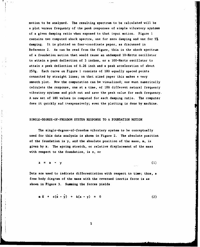
The single-degree-of-freedom vibratory system to be conceptually

used for this data analysis is shown in Figure 2. The absolute position

of the foundation is y, and the absolute position of the mass, m, is

given by x. The spring stretch, or relative displacement of the mass

with respect to the foundation, is z, or

z = X - y (1)

Dots are used to indicate differentiation with respect to time; thus, a

free body diagram of the mass with the reversed inertia force is as

shown in Figure 3. Summing the forces yields

m *+ C(xy) - k(x- y) = 0 (2)

Writing Equation 2 in terms of the relative displacement, z, defined in

Equation 1 yields

m * + cz + kz = -my (3)

By dividing by m, and using the traditional definitions and symbols in

Reference 11 given below

w + k (4a)

c = 2 m w (4b)

c/c (4c)

one obtains

S+ 2C w .+ w2z Z- (5)

Equation 5 gives the dyuamics of the simple system in terms of its more

interpretable characteristics, i.e., its undamped natural frequency, w,

and its damping ratio, C. It non-sizes the equation; all single-degree-

of-freedom systems with the same natural frequency and damping ratio

:must respond identically to the same transient acceleration. All shocks

or earthquakes are transient motions, which can be described in terms of

their transient accelerations. Thus, their effect on single-degree-of-

freedom systems is an excellent way of organizing or classifying their

capability to damage equipment.

The right hand side of Equation 5, the Y, or input to the equation,

will be a list of values. Solutions for Equation 5 will be developed

that generate a list of z's that result from the input. The theory will

also give us equations for x, z, and z once the list of z's has beea

found.

Several approaches exist for deducing the solution of Equat.ion 5

for a transient input, which is what is needed here. A good form, the

Duhamel integral form, is developed in most vibration texts; Thomson

6

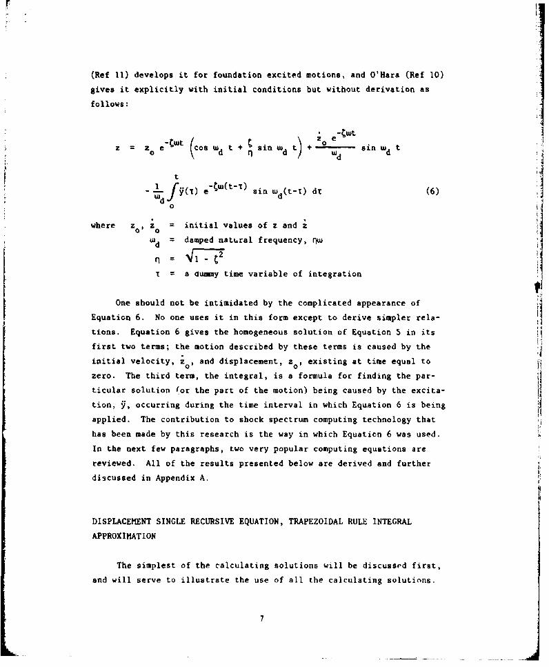
(Ref 11) develops it for foundation excited motions, and O'Hara (Ref 10)

gives it explicitly with initial conditions but without derivation as

follows:

-Cwtc~~~t C

z =zo e •t Wd t + sin +s W d dt

tI ..M e sin wd(t-i) dt (6)_d

where zo, z° = initial values of z and z

Wd = damped natural frequency, rw

T = a dummy time variable of integration

One should not be intimidated by the complicated appearance of

Equation 6. No one uses it in this form except to derive simpler rela-

tions. Equation 6 gives the homogeneous solution of Equation 5 in its

first two terms; the motion described by these terms is caused by the

initial velocity, Zo, and displacement, zo, existing at time equal to

zero. The third term, the integral, is a formula for finding the par-

ticular solution (or the part of the motion) being caused by the excita-

tion, Y, occurring during the time interval in which Equation 6 is being

applied. The contribution to shock spectrum computing technology that

has been made by this research is the way in which Equation 6 was used.

In the next few paragraphs, two very popular computing equations are

reviewed. All of the results presented below are derived and further

discussed in Appendix A.

DISPLACEMENT SINGLE RECURSIVE EQUATION, TRAPEZOIDAL RULE INTEGRAL

APPROXIMATION

The simplest of the calculating solutions will be discussed first,

and will serve to illustrate the use of all the calculating solutions.

7

It was first presented by Lane (Ref 8) and is in current use by most of

the aerospace community (Ref 4,12,13). The result is given below

ail 5 zi-2 + 16 z i- Yi- (7)

where the constants are given by

el5 = - •2th (7a)

isi

f1 6 = 2 e cos wd h (7b)

-h e"• sin wd h-he (7c)

ud

and where h is the time interval between samples of j. This is derived

in Appendix A as Equation A-lia.

The use of Equation 7 can be envisioned as follows. Consider that

for a given damping value, one wants to com~ute the peak z for some

frequency w V The constants a 15 ' a 1 6 ' and yI are first calculated.

Then is substituted into Equation 7 with z1 and z° equaling zero.

This yields a value for z2 . Next 2 and z2 are used to compute z3 with

zI again taken equal to zero. The value z4 is calculated from Equation 7

by using Y3 ' z3 ' and z2 ; and, thus, the process of calculating the z's

from the Y's continues. At each step of the computation, each newly

computed value of z is tested to see if it should replace what up until

that time has been the most positive and negative values. The absolute

largest of the two is the maximum. When the processing of the list of

Y's has been completed and the maximum z found, one has found the maximum

"during" values of z for that frequency. This process is repeated for

each frequency at which a shock spectrum value is desired.

One can refer to Equation 7 as a displacement recursive equation

for use with equally spaced digitized values of acceleration. The list

of displacements computed therefrom completely defines the resulting

motion. In Appendix A it is shown that if the velocity at any time is

desired, it can be computed from these displacement values as follows

8

a= G11 zi-I + a12 zi + ¥2 Yt (7d)

where the constants are given by

all = -(q W e'C•"•)/Csin rpaih)

S a w(l/tan rul - )-12

Y2= - h/2

If the relative acceleration, •i' is of interest, it is obtained by

using the values z and Yi' along with the computed value of zi in

Equation 5, which gives

2 C w w2 z'1 (7e)

If the absolute acceleration is desired, one notes from Equation I that

j =i i+ Vi(f

and, thus, from Equation 7e one finds

i= "2 w "w 2 z2 (7g)

Equations 7, the aerospace industry equations, are a complete set.

References 4 and 13 give Fortran program lists for their use. As men-

tioned in Appendix A, the apparent crudeness of the approximate integra-

tion meth.d was not made clear until Reference 4 was published in 1973.

Nothing has been written criticizing these equations, including Reference 4,

except that they nre completely ignored by the respected earthquake

analysis community (Ref 3 and 7). Reed (Ref 13) compares several com-

puting approaches and finds these equations inaccurate for coarse sampling

rates, but otherwise acceptable. The computational approach advocated

9

" • " " " " .. . ... .. .. . ... . .. .i ....... .. ....... . . ...... .. .. .. . . ... . . i -1M....E N •'

here resulted from trying to reconcile this computing approach with that

of References 3, 7, and 10. A suitably timple theory was found for

transforming the conventions), equations (Ref 3 and 10) into a single

displacement recursive equation so that simplicity of a single equation

could be retained along with the accuracy of the more conventional

integration approximations.

DISPLACEMENT AND VELOCITY PAIR OF RECURSIVE EQUATIONS, ACCELERATION

APPROXIMATED AS A STRAIGHT LINE IN INTEGRAL

The more conventional equations referred to above were first pre-

sented by O'Hara (Ref 10) in 1962 and then independently again by Nigam

and Jennings (Ref 3) in 1968. They approximate the acceleration by a

straight line between the sample points and then integrate the integral

of Equation 6. This yields a pair of equations for processing the data.

They are derived in Appendix A as Equations A-18c and A-18d and are as

follows

zi = aI + a2 i-I + a29 Yi-l + a 3 0 Y1 (Sa)

= a 4 zi-I + a 5 1-I + a 3 1 Yi- + a 3 2 Yi (8b)

The constants, which are a complicated expression, but of the same

variables as in Equation 7, are given in Appendix A as Equations A-4c,

A-4d, A-4f, A-4g, A-18i, A-18j, A-18k, A-181. In this computing method,

two outputs, both z and i, must be computed for each step, and then used

in the next. Since both z and z are being constantly computed, it is a

simple matter to use Equation 7g to compute the acceleration of the

mass, 9, at each point if desired. This is the procedure currently in

use for most of the U.S. earthquake data (Ref 7), and hence is a highly

respected approach. Note that for each step, or for each point of input

data, eight multiplications and six additions are required. What was

found during the course of this work was that the above pair could be

exactly reduced to a single equation; this results in each step only

requiring five multiplications and four additions.

10

ItDISPLACEMENT SINGLE RECURSIVE EQUATION, ACCELERATION APPROXIMATED AS A

STRAIGHT LINE IN INTEGRAL

In Appendix A it is shown that with some shifting of the indices,

one can combine Equations 8& and 8b into the single equation given below

Zi s15 zi-2 16 i-I 24 Yi-2 + a2 5 Yi-l 1 ÷26 Yi (9a)

The constants again are complicated, but easily computed and are given

in Appendix A as Equations A-lOe, A-lOf, A-19b, A-19c, and A-19d. Note

that the constants applied to the z's are the same as those of Equation 7,

Lane's result (Ref 8). No matter how sophisticated an approximate

integration is, these same two constants appear. It does seem more

reasonable that three input values are required for each step, including

the value, Yi' for the time at which the output, zi, is being computed.

As was the case previously, the data or list of Vi's is marched

through Equation 9a, which yields a z. for each 91. If the velocity at

any point is desired, it can be computed as shown in Appendix A,

Equation A-20a, from the z's as follows

= a11 zi-1 + a 12 z + a2 7 Yi-I + a2 8 Vi (9b)

The constants are given in Appendix A as Equations A-10, A-lOc, A-20b,

and A-20c. If the absolute acceleration of the mass, xif is desired, z

is computed and used with zi in Equation 7&.

RESIDUAL SPECTRUM CALCULATION

As has been discussed, the spectrum computation consists of exciting

the theoretical model of Figure 1, which is described by the differential

Equation 5, by means of a calculation algorithm (such as Equations 7, 8,

or 9) with the excitation given as a sequence of equally spaced values.

11

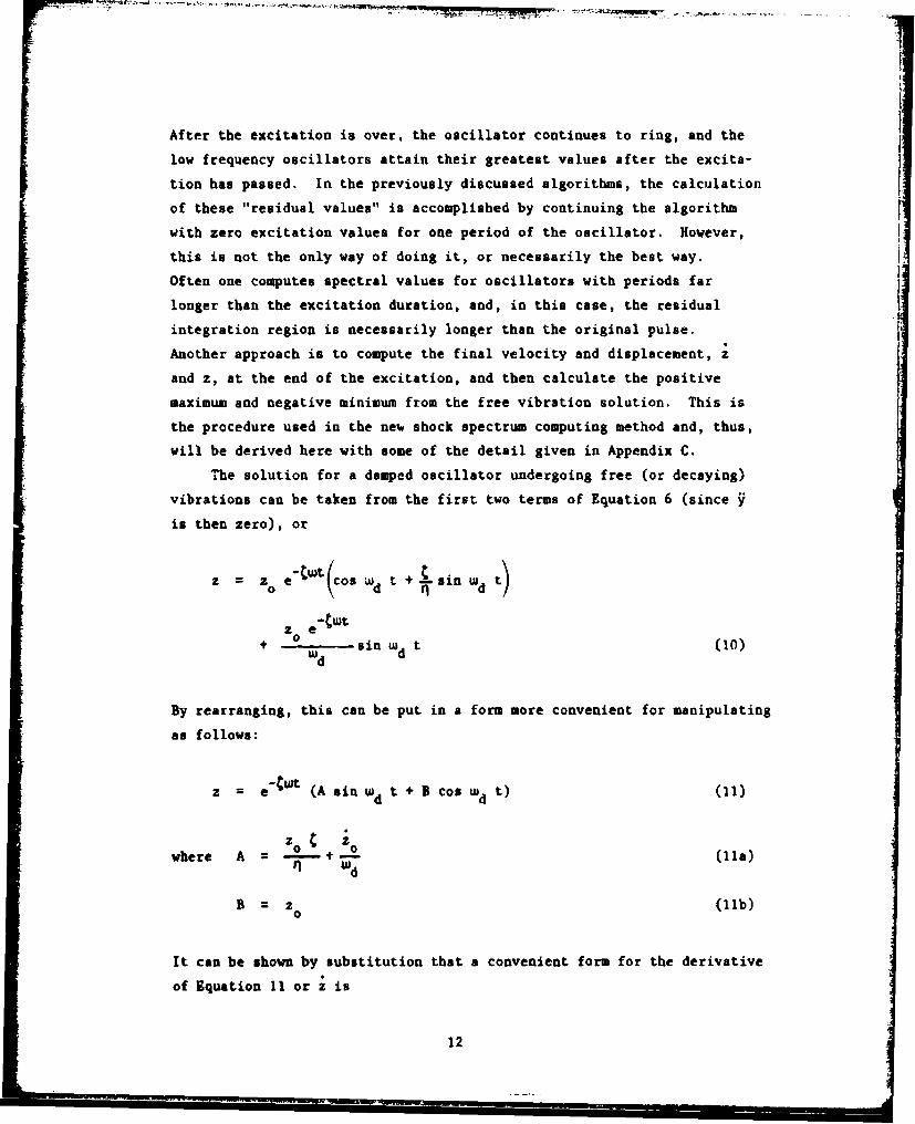
After the excitation is over, the oscillator continues to ring, and the

low frequency oscillators attain their greatest values after the excita-

tion has passed. In the previously discussed algorithms, the calculation

of these "residual values" is accomplished by continuing the algorithm

with zero excitation values for one period of the oscillator. However,

this is not the only way of doing it, or necessarily the best way.

Often one computes spectral values for oscillators with periods far

longer than the excitation duration, and, in this case, the residual

integration region is necessarily longer than the original pulse.

Another approach is to compute the final velocity and displacement,

and z, at the end of the excitation, and then calculate the positive

maximum and negative minimum from the free vibration solution. This is

the procedure used in the new shock spectrum computing method and, thus,

will be derived here with some of the detail given in Appendix C.

The solution for a damped oscillator undergoing free (or decaying)

vibrations can be taken from the first two terms of Equation 6 (since j

is then zero), or

0-Ct~o Zot+ i Wd tz -Cwt (t0 mwd t (10)

By rearranging, this can be put in a form more convenient for manipulating

as follows:

z = e"Cwt (A sin wd t + B cos wd t) (11)

where A = -- 4-C+ d (01a)1 d

B z0 (1ib)

It can be shown by substitution that a convenient form for the derivative

of Equation 11 or z is

12

w= eCwt [A cos(wd t + 6) B sin(wd t + 6)) (12)

where sin6 = (12a)

cos 6 = (12b)

n C2 (12c)

wd = w (12d)

Since Equation 11 is a damped vibration or at the most with • = 0, a

constant vibration, both the most positive and the most negative value

must occur in the first cycle or at t = 0. Thus, z and zmin must beS~~max n

pursued in the first cycle. If not, when t 0, these occur when z

equals zero or when

A cos(wd t + 6 ) B sin(wd t + 6) (13)

If

= Wd t + 6 (14)

one seeks • such that

A cos P B sin 0 (15)

or

tan p = A/B (15a)

and also seeks two values 1 and 2 such that the results (wdt)1 and( adt)2 are between zero and 2n. Clearly, 01 and 02 are consecutive

angles at which the velocity goes to zero; thus (since the tangent goes

through zero every n radians),

13

P2= 1 (16)

Now one must go through an amour.r of detail to assure the finding of the

very first time after time equals zero that z equals zero. Nine cases

must be considered as indicated:

A>O A:O A<O

B>0 I II III

B = 0 IV V VI

B < 0 VII VIII IX

This is done carefully in Appendix C. The results are given below as

the set of "if" statements used in programing the computation.

1. If both A and B are zero, no residual response results.

2. If not, and A = 0, then P 0. (17a)

3. If not, and B = 0, then 1 = (7

4. If not, and A and B have the same sign,

A, = Tan-1 (A/B) (17c)

5. If not,

Pl = n - Tan-1 (-A/B) (17d)

Nov with this value of P1, one final test is required. If, and only if

P e < 0 (17e)

one must add R to P•, or

P (PI)old + n (170)

14

Now with the acceptable value of PI, (wdt)l can be obtained with Equation 14

as follows

(Wdt)l = 01 - 6 (1g)

The second value of (wdt) is obtained from

(wdt) 2 (Wdt) + n (17b)

These values of (wdt)l and (wdt) 2 are substituted successively int o

Equation 11, which will yield values for zmax and zmin. These values

are compared with z to make sure it is not greater than z or less

than Zmin, and, thus, the residual spectrum values are computed. Sub-

routine RESID listed at the end of Program SPCTRH in Appendix B uses

this procedure to compute the residual spectrum values.

Some additional explanation of the need for the residual spectrum

computation procedure is given here, since the previously mentioned

programs do not go to this trouble. To get the residual response, one

must first use a numerical method (such as Equations 7, 8, or 9) to find

the displacement and velocity (z and z ) at the end of the "during"

portion of the response. The other computations continue the numerical

procedure to find the residual maximum values. This procedure uses a

theoretically exact method to compute the values; it is faster, more

accurate, but a little clumsier to program.

THE COMPUTER PROGRAMS

Appendix B gives the Fortran listings for the two computer programs

used in the preparation of shock and response spectra by this new method.

The first, SPCTR!, computes the shock spectrum and lists as output the

values of the maximum and minimum displacement and pseudovelocity for

each frequency considered. The second, PLTVLF, is the program used to

plot the maximum, positive or negative shock spectrum on the four-

coordinate paper. Note that the precise frequencies used for calculation

5I

are selected by the program so that they will be equally spaced when

plotted logarithmically. Appendix D documents the logic for this section

of program SPCTRM. Otherwise the steps and symbols of the program

coincide with the report body and appendices, and should be completely

readable. The programs are in current use on a CDC time-sharing terminal;

the plotting is done on an interconnected Hewlett Packard Model 7202A

Graphic Platten. The format statements show the form of the input data.

The programs interrogate the user and, thus, supply the needed documen-

tation.

COMENrrs

The Accuracy of the Algorithms

Equation 9a is more accurate than any others thus far published.

Because these recursive calculating equations use previously computed

results for each succeeding step, they propagate any errors introduced.

Thus, if fewer multiplications and additions are required for each step,

there is less opportunity for error accumulation due to roundoff and

subtraction of nearly equal values.

Of the algorithms reviewed, Equation 7, the "trapezoidal" approach,

has the fewest multiplications and additions. However, it assumes each

factor of the integral is constant during the integration. If one

graphs the value of the factors over the integration interval and then

compares an estimate of the integral of their product with that assumed

by the algorithm, the crudeness of the approximation becomes apparent.

Thus, the "trapezoidal" rule approach was discarded because of these

initial assumptions.

Conversely, if one graphs the values of the factors similarly with

the straight line integration approach, one can infer a convergence to

the "true" value as the steps become smaller. Such an examination even

leads one to assume the straight line approach is exact; such a comment

was even made in Reference 3. That is why most of the algorithms use

16

{iithe straight line approach. Of these the new single recursive equation

developed here has by far the fewest multiplications and additions and,

thus, is the most accurate.

A rigorous study of the accuracy of the approaches has not been

undertaken, and would certainly be welcomed. However, perfunctory

accuracy statements that pretend to bound the error by referring to

higher derivatives of the input are not applicable to digitized data.

Nor is there any way in which one can construe the data to be composed

of low order polynomials. As is discussed further in Appendix A, one

does not want to sample any coarser than about 10 points per cycle of

the highest frequency present. At this high a sampling rate, the straight-

line-between-the-points assumption makes an accurate appearing plot of

the data, which leaves one to believe the integration has been adequately

approximated.

Allowable Frequency Ranges

This new program, as well as all other shock spectrum computer

programs, has limitations on the frequencies for which it can compute

accurate shock spectrum values. The allowable frequencies are dependent

upon the sampling rate of the data used as iaput and upon the number of

digits the particular computer uses in performing its arithmetic opera-

tions. The high frequency limit for the programs discussed in this

report is one tenth of the sampling rate. This assures a 5% accuracy

and is discussed by most authors (Ref 3).

That a low frequency limit exists has not been published up to now.

The constants that apply to the input data in Equations 7, 8, and 9a

contain sines and cosines with arguments that become very small at low

frequencies and lead to the subtraction of nearly equal numbers (e.g.,

equal to the 12th or 13th digit in a 14-digit number). At very low

frequencies this can lead to the computer generating ridiculous values

off by a factor of ten or more. Time did not. permit a thorough investi-

gation of this effect, but an empirical testing of the constants did

indicate that for the computer used, which calculates to 14-digit accuracy

in single precision, accuracy could be maintained for frequencies as lowas one eight-thousandth of the sampling rate.

17

These frequency limitations are more completely discussed in

Appendix A. In symbols, the range of allowable frequencies for the

programs can be expressed as

f10 s -" 1 8000 (18)

Thus, for data that have been sampled at 10,000 points per second, one

could compute shock spectrum values for frequencies as high as 1,000 Hertz

and as low as 1.25 Hertz. The current program does not impose this

restriction; it is the responsibility of the user.

SUMMARY

The body of the report has presented a background in shock spectrum

calculation methods applicable to digital computation that has not been

available. In general terms in the text and in detail in Appendix A,

the two most popular methods and a new method are described, defined,

and completely derived. This new method decreases the numbers of addi-

tions and multiplications required by 4O0 and, thereby, increases accuracy

while decreasing cost. The main purpose of the report is to document

this new method and make it available. Appendix B gives computer program

lists for this new method.

There are still unresolved questions and certainly room for improve-

ment; these matters are discussed. In particular, a new potential.

source of inaccuracy was discovered in trying to extend to earthquake

frequencies data that had been sampled for explosion frequencies. The

only way one can compute spectra for the very low earthquake frequencies

is to have the data digitized at an appropriate sampling rate.

The author believes that a greater understanding of the shock

spectrum is valuable for evaluating equipment installation in dynamic

environments. Here plotting of the shock spectrum on four-coordinate

paper gives a vastly improved appreciation of the damaging capacity of a

given environment. Required rattlespace stands out and, to the extent

18

that one can approximate the gross natural frequency of the equipment on

its support, the peak breakaway forces can be estimated. A considerable

increase in safety and facility hardness from the effects of explosion

and earthquake is available inexpensively from increased understanding

and use of the shock spectrum.

Finally, this study of the shock spectrum analysis of sampled

acceleration time histories not only reduced and clarified the required

calculations, it also provoked several ideas for even further reducing

the program size. It must be assumed that soon small calculators will

be doing the analysis. Inexpensive digitizers and plotters will follow,

and all will have access to many new tools for intelligent use of the

data that now is only plotted.

ACKNOWLEDGENT

The author wishes to acknowledge the help of Dharam Pal of the

Civil Engineering Laboratory in the development of this work. Many of

the fundamental analysis ideas were his, as we worked together during

the initial stages of this calculation procedure and program development.

The work was made possible through the support of the Raval Facilities

Engineering Command Code 03 in Alexandria, Virginia. In particular,

Herbert Lamb of that office was the program manager in charge of this

work. His encouragement and support were, in a large measure, the

reason for the forthcoming successful completion of this project.

REFERENCES

1. Civil Engineering Laboratory. Technical Memorandum M-63-76-12:

Shock spectrum calculation from sampled acceleration time histories, by

H. A. Gaberson and D. Pal. Port Hueneme, Calif., Sep 1976.

2. Civil Engineering Laboratory. Interim Report No. YF53.534.006.01.017:

A design method for shock resisting equipment installation, by H. A.

Gaberson. Port Hueneme, Calif., Apr 1975.

19

3. California Institute of Technology, Earthquake Engineering Research

Laboratory. Digital calculation of response spectra from strong-motion

earthquake records, by N. C. Nigam and P. C. Jennings. Pasadena, Calif.,

Jun 1968.

4. D. L. Cronin. "Numerical integration of uncoupled equations of

motion using recussive digital filtering," International Journal for

Numerical Methods in Engineering, vol 6, 1973, pp 137-152.

5. J. B. Vernon. Linear vibration and control system theory. New

York, N.Y., John Wiley and Sons, Inc., 1967, pp 251-252.

6. Naval Ordnance Laboratory. Report No. NOLTR-68-37: Shock spectra

and an application to antillery projectile shock, by P. S. Hughes.

White Oak, Md., Mar 1968.

7. National Information Service. Earthquake engineering computer

applications, Programs 06-573, SPECTR, and 08-573 SPECEQ/SPECUQ, Earth-

quake Engineering/Computer Applications, Davis Hall, University of

California. Berkeley, Calif., Listing of Apr 1978.

8. Naval Research Laboratory, Shock and Vibration Information Center.

Digital shock spectrum analysis by recussive filtering, Shock and Vibra-

tion Bulletin V33, Section 2, by D. W. Lane. Washington, D.C., 1964,

pp 173-181.

9. E. I. Jury. Theory and applications of the Z-Transform Method. New

York, N.Y., John Wiley and Sons, Inc., 1964.

10. Naval Resea.ch Laboratory. Report No. 5772: A numerical procedure

for shock and Fourier analysis, by G. J. O'Hara. Washington, D.C., Jun

1962.

11. W. T. Thomson. Vibration rheory and applications. Englevood

Cliffs, N.J., Prentice-Hsll, Inc., 1965, pp 56 and 104.

20

12. Naval Research Laboratory, Shock and Vibration Information Center.

SVM-5: Principles and techniques of shock data analysis, by R. D. Kelly

and G. Richman. Washington, D.C., 1969.

13. Naval Ordnance Laboratory. NOLTR 70-243: Comparison of methods

used for shock and Fourier spectra computations, by R. S. Reed, Jr.

Silver Spring, Md., Nov 1970.

14. L. A. Pipes. Applied mathematics for engineers and scientists, 2nd

ed. New York, N.Y., McGraw-Hill Book Company, 1958.

15. Sandia Laboratories. Report No. SAND-74-0392: Shock spectra, by

R. Rodeman. Albuquerque, N.M., Oct 1974.

16. R. S. Burrington. Handbook of mathematical tables and formulas,

5th ed. New York, N.Y. McGraw-Hill Book Company, 1973.

I

7171 2

=1.i104

II

S102 3•

_.-",l,

/X~~ ~ ~ A, X,_A-\ W

1.0

I.0- Y

U.A.

1.0 10 10 2 10 3 104

FREQUENCY (H,)

Figure 1. Relative displacemer shock spectrum plottedon four-coordinate paper. Upper curve isundamped, the lower curve is for 5% damping.

22

Figure 2. Single-degree-of-freedom vibratory system.

-4*4

Figure 3. Free body diagram.

23

fI 23

Appendix A

DERIVATION 0F RECURSIVE EQUATIONS

DERIVATION APPROACH AND NEW 8YMBOLS

As has been discussed in the text, one seeks a solution of Equation 5,

1+2Cwz ,w 2 z + -2 w (5)

applicable to a list of closely and equally spaced values of the input

foundation acceleration, Y. Hence, three such solutions of Equation 3

will be developed that apply from one excitation point to the next.

They will be recursive calculating equations, through which the input

data are successively passed, thereby yielding a list of output values,

z. The text equations and definitions I through 6 will be used. The

approach of this Appendix is tn give s general beginning leading to two

known results and the Lew result.

The Duhamel integral solution, Equation 6, is the point of departure.

The derivative of this solution with respect to time is needed, and this

must bo done carefully since t is a limit of, and occurs within, the

integral. Pipes (Ref 14) explains this carefully, and following his

instruction one obtains

.o2 e-cwt t

e sin wd t + * o'

t

,+ cos Wd t) I - y(€) .in ,(t-,)0

+ f cos wd(t-T)) di (A-i)

25 4S h UiIw I

Fr

Consider applying Equations 6 and A-I from one value of • to the next;

i.e., from 90 to Y,. As can be read, the equations presume z0 and z0

are known. Equation 6 would give z,, and Equation A-i would give zl.

To clarify what follows, some new symbols must be defined. The

time interval between the equally spaced values will be h. Equations 6

acd A-I are to be applied when t equals h. Therefore, define

S"wh sin wd h (A-2a)

a e- Cos ud h (A-2b)

h

Ol : fy (t) •-tw(h-T) sin wd(h-t) dt (A-2c)

0

h

01 0 /y(•1 e"cw(h-t) cos wd(h-r) dr (A-2d)0

Using these now symbols, Equations 6 and A-i become

z! + (A-3a)

* (--+-)-.s01 - (A-3b)

Note that as these equations are applied to the input list of Y's,

h, w, C, wd, i, X, and * are constants. If subscripted a's a•e to

represent constants, Equations A-3 become

Z z a1 I 0 a2 0 + az 3 S 01 (A-4-)

1 = a 4 z0 + a5 Z + a6 S01 + a 7 CO (A-4b)

where a X+ (A-4c)

26

F

(A-4d)

- 3 I(A-4e)a3 rl W

a •.W_.. (A-4f)

u5 •- •-•+ X(A-4g)

a -(A-4h)

a 7 -l (A-4i)

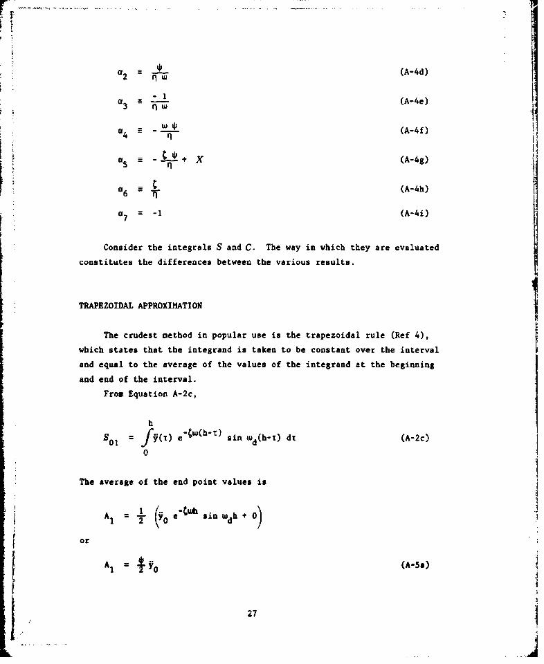
Consider the integrals S and C. The way in which they are evaluated

constitutes the differences between the various results.

TRAPEZOIDAL APPROXIMATION

The crudest method in popular use is the trapezoidal rule (Ref 4),

which states that the integrand is taken to be constant over the interval

and equal to the average of the values of the integrand at the beginning

and end of the interval.

From Equation A-2c,

h

S01 = f ( W sin wd(h-i) di (A-2c)

0

The average of the end point values is

iI.t~whJA I T e- uinwdh+ O0

or

A = (A-s.)

27

/i

Using this as the integrand in A-2c yields

S = h. (A-5b)

for the value of S 0 by the trapezoidal rule. To get the value of

C0 1 , consider

h

C01 = fy(T) e •h) cos wd(h-) di (A-2d)00

The average of the end point values is

2 = -L Yo coswdh+ (A-5c)

Using this as the integrand in A-2d yields

C = A x V +(A-Sd)

The point to note here is that in this case, and in the other cases

to be considered, the integrals, Sol and Col, are composed of constants

and input data values; no z's or output values. This can be seen more

clearly as follows.

By substituting these values of S01 and C01 , Equations A-5b and

A-Sd into Equations A-4a and A-4b, one obtains

= ÷1 z +a 2z 0 +a'$g (A-6a)

and

a= 4 Z0 +a5 z0 + U 0 YO +ai (A-6b)

where these new a's are defined to be

28

toh/ (A-60)3 3

h

-~(6 *~7 ) (A-6d)

aj a7 h/2 (A-6e)

Thus, it is seen that, upon evaluation of S01 and CO1, which become

products of constants and the input Y's, Equations A-4a and A-4b become

Equations A-6a and A-6b. These form a pair that are used together to

generate a list of both z's and z's, from the Y's. Assuming the a's

have been computed and the full list of the Y's is on hand, one would

start the calculating at Y , taking z0 and Z0 equal to zero, and proceed0Y

to zi. Knowing zi and zi, the pair of equations will yield zi+I and

z i a and so on.

With this in mind it is now possible to go back and combine the two

equations (A-4a and A-4b) into a single equation for zi alone, thereby

* elimirating the need to keep computing both z and z. This development

does tot require Z Transform Theory (Ref 8 and 9) and is more straight-

forward than the approach of Cronin (Ref 4).

DEVELOPMENT OF A SINGLE RECURSIVE EQUATION

One begins by solving Equation A-4a for z and defining new a's.0

This yields

Z a 8 Z0 + a9 z1 + a1 0 Sol (A-7a)

where as - a" (A-7b)

a9 (A-7c)r2

• a3a30 (A-7d)

2

29

Equation A-7a is next substituted into A-4b, which then becomes

Sz +a(a z +a9 zI a S1)1 a4 + o 5 a o a + 01O 1

+ 6SO ta7 CO (A-8a)601 7 01

By defining new a's, this can be written as

a 11 l 0o + a12 ZI + a 13 S01 + 14 C0 1 (A-Sb)

where al = 4 + a5 "S (A-Sc)

a12 = a 5 a9 (A-Sd)

@13 = a5 a10 + a6 (A-Se)

@1 a - 7 (A-Sf)

This is a very interesting result. It states that the velocity at point

1 is exactly given by zo and z, and the values of the two integrals.

Note that it does not require z

The next step is to realize that Equation A-l4a also applies between

points I and 2 equally as well as between points 0 and 1, and, thut, the

following can be written

2= 1 1+ 2 1 3 S 1 2 (A-9a)

The value of from Equation A-8b is substituted into this form, which

yields

z = 1 z1 + a2(a 2z + a2 z + a13 S0 1 + a14 CO1 ) (A-9b)

SS3 12

30

And finally by defining more a's, this becomes

z = a z + a z + a S + a S aC (A-9c)2 15 0 16 1 17 01 18 12 1901o

where a15 a2 a11 (A-9d)

a1 a1 + a2 a2 (A-9e)

a 1 7 £ a2 a13 (A-9f)

18 3

a a a (A-9h)19 2 14

Equation A-9c is the new result. Note that it is quite different

from Equation A-4a in that it requires no input velocity; thus,

Equation A-4b does not have to be computed along with it. It reduces

the number of computations and, thus, the accumulation of error. It is

therefore more accurate and economical. If the velocity is desired, it

can be calculated with Equation A-8b. As it stands it is exact. Approx-

imation will be introduced when the integrals are evaluated and by

round-off error accumulated in the calculations.

Before using Equation A-9c with various approximations for the

values of the integrals, Sol and C0 1 , many of the a values will be

required and so the most important ones are listed below.

a = e-2twh = -Cwha11 l sin wd h (A-lO)

a12 = W - = w C (A-lb)

121X _ I

a13 = tan wd h (A-10)

a14 = -1 (A-10d)14

a 15 =-e 2(A-l0e)

+ 31

= 2X (A-10f)

a = (A-lOg)17

_la - (A-lOh)

a19 -(A-10i)

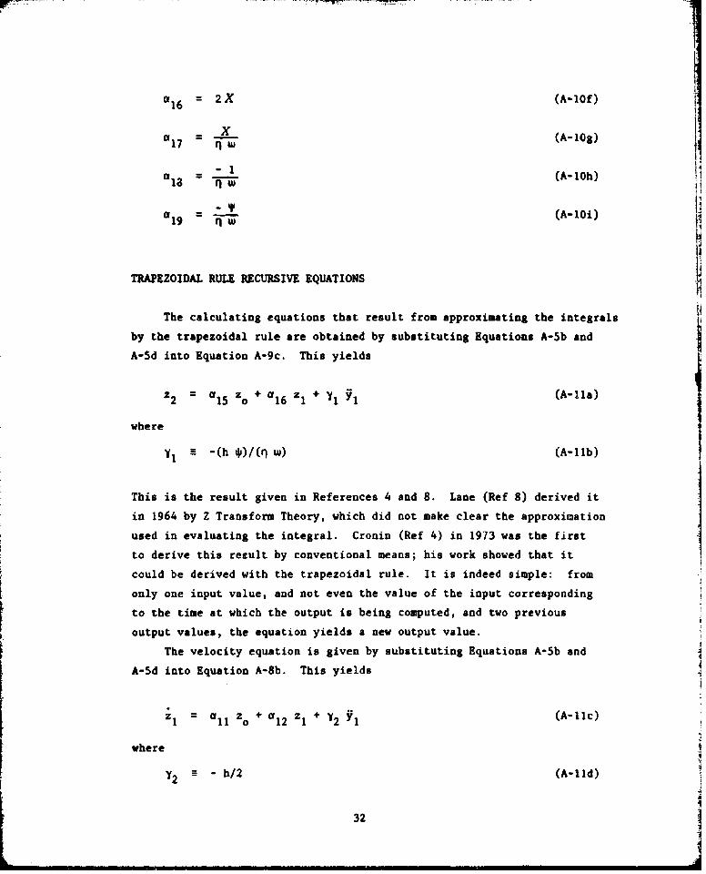
TRAPEZOIDAL RULE RECURSIVE EQUATIONS

The calculating equations that result from approximating the integrals

by the trapezoidal rule are obtained by substituting Equations A-Sb and

A-Sd into Equation A-9c. This yields

22 = 15 + a 1 Y (A-Ila)

where

= -(h *)/(r w) (A-11b)

This is the result given in References 4 and 8. Lane (Ref B) derived it

in 1964 by Z Transform Theory, which did not make clear the approximation

used in evaluating the integral. Cronin (Ref 4) in 1973 was the first

to derive this result by conventional means; his work showed that it

could be derived with the trapezoidal rule. It is indeed simple: from

only one input value, and not even the value of the input corresponding

to the time at which the output is being computed, and two previous

output values, the equation yields a new output value.

The velocity equation is given by substituting Equations A-Sb and

A-Sd into Equation A-8b. This yields

S a1 1 z0 +a 1 2 Z I+2 Yl (A-llc)

where

2 a "h/2 (A-lid)Y2

32

II

This equation is used to compute a velocity if required; e.g., the final

velocity is required as input to the residual response calculation.

Reiterating, Equation A-1la is used to compute a list of a's from the

list of Y's; i.e., if Yl is the first non-zero point, Equation A-1Ia

yields z2 as the first non-zero output value. Next Y2 and z2 are used

to compute z3; next Y3 * 23' and Z2 are used to compute z 4 , etc.

Equation A-lia written for the general (n+l) point is

z+l a15 Z + a Z + ¥1Yn (A-lie)U+ 5n-i 16 na

which is a more common way of writing a recursive equation.

STRAIGHT LINE ACCELERATION APPROXIHATION IN INTEGRAL

There are several other approaches one could take in evaluating the

integrals S and C. Cronin (Ref 4) suggested considering the values of

the integrand at three consecutive points as defining a parabola and

then integrating the parabola so defined. Rather than approximate the

whole integrand by an approximating function, O'Hara (Ref 10) in 1962,

and Nigam and Jennings (Ref 3) in 1968, both derived the pair of computing

equations that result from Equations A-4a and A-4b when the acceleration

input is approximated as a straight line between two adjacent values.

They then integrated the product of the approximate acceleration function

and the remainder of the integrand. Vernon (Ref 5) in 1967 published an

unusual pair, similar to Equations A-4a and A-4b, again with the straight

line acceleration approximation, except he chose to compute x and x as

output values (as opposed to z and z). Rodeman (Ref 15) in 1974 used Z

Transform Theory more accurately than Lane (Ref 8), approximating only

the acceleration as a straight line, and deriving a single recursive

equation with acceleration, i, as the output, as opposed to z. Thus,

the straight line approximation has a host of advocates. Except for

Cronin (Ref 4), none found the single recursive equation without Z

Transform Theory.

33

As to the accuracy of the straight line approximation, Referencc 3

calls the method "exact". O'Hara (Ref 10) gives formulas for approxi-

mating the acceleration by a parabola, which clearly has to be better

than a straight line. The philosophy taken here is that, if the sequeuce

of digits when plotted with straight lines connecting adjacent points is

a good visual approximation to the analog data, then the digitizing is

adequate for approximating the acceleration function with straight

lines.

To evaluate the integrals S0 1 and C01 with the acceleration taken

as a straight line between adjacent values, or go and Y1, let

S(a) = a b T (A-12a)

where

a M YO (A-12b)

b S (Y1 YO)/h (A-12c)

Equation A-12a is used in the definition of So 1 , Equation A-2c, to yield

h

S f01 = (a + b x) e•w(hT) sin wd(h-c) di (A-13a)

0

To integrate this expression, change the variable

u = h (A-13b)

Thus,

du = - di (A-13c)

and

S= h -u (A-13d)

For the limits, note from Equation A-13b that when

,= 0 u h (A-13e)

34

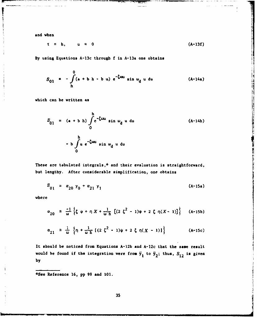
and when

= h, u 0 (A-13f)

By using Equations A-13c through f in A-13a one obtains

0

S 1 = -J(a + b h -b u) e sinwdudu (A-14a)

h

which can be written 4s

01 (a + b h) e"US Bin wd u du (A-14b)

0

-fu e•Wu sin wd u du

These are tabulated integrals,* and their evaluation is straightforward,

but lengthy. After considerable simplification, one obtains

S 0 1 = a2 0 YO + a21 Yl (A-15a)

where

120 + n(2 1)* +2Cq(X- 1)] (A-15b)

21n + [(2 C2 - 1) + 2 C r(X - 1)4 (A-15c)

It should be noticed from Equations A-12b and A-12c that the same result

would be found if the integration were from yV to V2 ; thus, S 1 2 is given

by

*See Reference 16, pp 99 and 101.

35

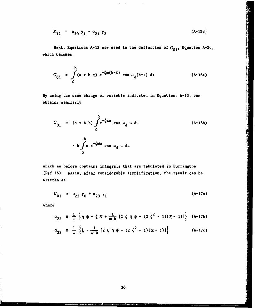
S 12 C120 YI+of21 Y2 (A- 15d)

Next, Equations A-12 are used in the definition of C0 1 , Equation A-2d,

which becomes

C f1 = f(a + b t) •"w(ht%) cos wd(h-x) di (A-16a)

0

By using the same change of variable indicated in Equations A-13, one Fobtains similarly

h

C01 a (a + b h)/fe"twu cos wd u du (A-16b)0

h- bfu e"twu cos Wd u du

0

which as before contains integrals that are tabulated in Burrington

(Ref 16). Again, after considerable simplification, the result can be

written as

C =0 22 YO + a23 Yi (A-17a)

where

a22 - 2

23 - -L (2 t n " (2 C2 1)(X_ 1)11 (A-17c)

36

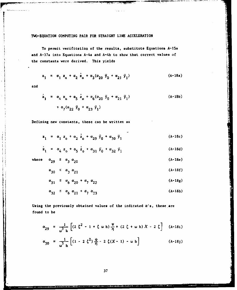
TWO-EQUATION COMPUTING PAIR FOR STRAIGHT LINE ACCELERATION

To permit verification of the results, substitute Equations A-15sa

and A-17a into Equations A-4a and A-4b to show that correct values of

the constants were derived. This yields

1 o 2 20 3(a20 0 21 (y+A-8a)LO

and

a 5 z +6 0 of + a y) (A-18b)l 4 0o o 0 (620 90+ 21 Y

+ a 77(a22 YO + a2 3 Yl)

Defining new constants, these can be written as

=, a z0 + a z +- a2 0+ 3 jr (A-18c)1l 0 2o 0o 29 YO+ 30 Y

z + a o + a (A-18d)

54 0 031 YO+a32Y1

where a29 a a320 (A-18e)

a30 a3 a (A-18f)30 3 21

031 = 06 020 +07 022 (A-18g)

a a a21 a (A-18h)

Using the previously obtained values of the indicated O's, these.are

found to be

029 = (2 - I wh)-±+ (2 + w h) X - 2 ] (A-18i)

130 --- [(1 - 2 2 C(X- 1) hw (A-18j)

37

3l - - [1 - + w h) -X (A-18k)

a 3 2 X -- +XI (A-181)

These are the equations used in Reference 3, and the constants

agree, except for two typographical misprints, which are corrected in

the Fortran program listing. One might at first think these expressions

adequate if both the relative velocity and displacement are desired.

However, such is not the case because the recursive process would then

involve more calculations and, thus, a greater accumulation of error.

The equations are only given here for completeness.

NEW SINGLE RECURSIVE EQUATION FOR A STRAIGHT LINE ACCELERATION

APPROXIMATION

Now the results of evaluating the integrals S 0 1, S 1 2 , and CO1 , with

the acceleration taken as a straight line between the digitized values,are obtained by merely substituting Equations A-15 and A-17 into

Equation A-9c. The result can be arranged as follows

Z a z + a Z + a (A-19a)z2 is5 0o 16 1 a24 YO+a25 V1+a26 Y

where the new constants are found to be

[2 C X - e'2 h(2 t + w h) + (I-2 2) (A-19b)

2 -~.[whX. (1 -2 •2• C(l . e-2Cta)] (A-19c)24 = na25 W3 h

12 [11 - 2 2) + 2 C(( -X) - w h (A-19d)a26

38

and the first two constanLs are repeated here for convenience

@15 (A-lOb)

a16 2X (A-10i)

It is hoped that the reader has observed that the indices 0, 1, and

2 on the z and 9 values do not restrict this result to the first three

points of the data list, i.e., they are perfectly general; in fact, to

better conform to other writings on recursive calculating equations,

Equation A-19a can be written for calculating the ith value as

zi = a15 zi-2 + a16 4i-1 + a24 Yi-2 + 025 Vi-1 + *26 Vi (A-19e)

Though it is a trivial observati~n, especially after going through the

algebra three times, the reader will note on his first time through that

42 +X2 = e-2twh (A-19f)

is a group that recurs.

The velocity equation for calculating velocities from the computed

displacements is similarly obtained by substituting Equationx A-15 and

A-17 into A-8b which again, after simplification, can be written as

i = llz i-I 1+ 12 zi + a27 Yi-1 + '28 Yi (A-20a)

where

a- 27 (2 • + w h) - 2 C2 + (A-20b)27

1 2 C e-2twh -(w h 2 C - I (A-200@28 -- (W2 h

39

and from the previous results

G|2w

a 12 W( t (4-10)

Equations A-19e and A-20a are the new result. Equation A-19e is

the equation that marches through the data yielding relative displace-

ments, zi's, from only previously computed zi's and excitation values.Note also that each step requires only five multiplications and four

additions. It is theoretically identical to using both Equations A-18c

and A-18d, but avoids relative velocity as an intermediate result.

Equation A-20a is the velocity calculation; it exactly calculates the

velocity at any desired point irom computed displacements and input

values.

Incidentally, it is more straightforward to deduce Equations A-18c

and A-18d directly from the original differential Equation 5 by sta.ting

with the straight line acceleration approximaticn in the right-hand side

and obtaining the needed particular solution by undetermined coefficients.

This is the technique of Reference 3. Then Equations A-18c and A-18d

are transformed to Equation A-19e by going through the steps of

Equations A-7 to A-9 for this specific case rather than for the general

case.

FIRTHER COMMENTS ON ACCURACY AND REMAINING PROBLEMS

Some comments were made in the report body on accuracy, and they

are applicable here. Additionally, one might say that if both the

relative displacement and the relative velocity are desired, one might

just as well use the two-equation approach of References 3 and 10. That

would be less accurate because the propagation of the solution through

the data would require eight as opposed to five multiplications per step

and six as opposed to four additions per step. Accuracy would suffer.

40

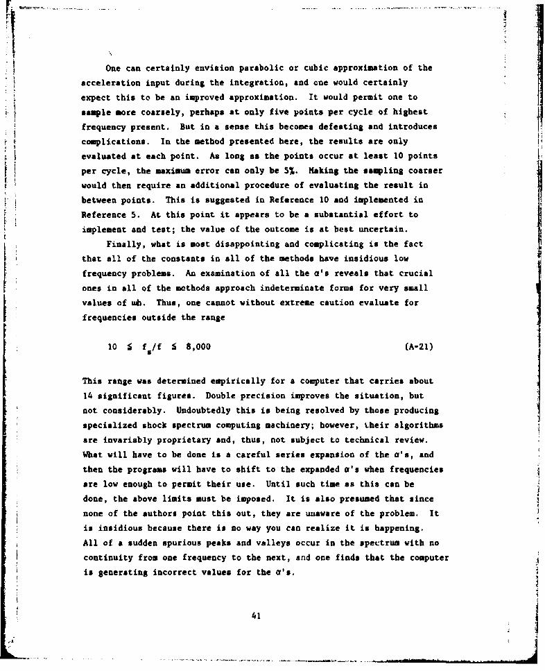
One can certainly envision parabolic or cubic approximation of the

acceleration input during the integration, and cne would certainly

expect this to be an improved approximation. It would permit one to

sample more coarsely, perhaps at only five points per cycle of highest

frequency present. But in a sense this becomes defeating and introduces

complications. In the method presented here, the results are only

evaluated at each point. As long as the points occur at least 10 points

per cycle, the maximum error can only be 5%. Making the sampling coarser

would then require an additional procedure of evaluating the result in

between points. This is suggested in Reference 10 and implemented in

Reference 5. At this point it appears to be a substantial effort to

implement and test; the value of the outcome is at best uncertain.

Finally, what is most disappointing and complicating is the fact

that all of the constants in all of the methods have insidious low

frequency problems. An examination of all the a's reveals that crucial

ones in all of the methods approach indeterminate forms for very small

values of wh. Thus, one cannot without extreme caution evaluate for

frequencies outside the range

10 S f /f S 8,000 (A-21)

This range was determined empirically for a computer that carries about

14 significant figures. Double precision improves the situation, but

not considerably. Undoubtedly this is being resolved by those producing

specialized shock spectrum computing machinery; however, Lheir algorithms

are invariably proprietary and, thus, not subject to technical review.

What will have to be done is a careful series expansion of the a's, and

then the programs will have to shift to the expanded a's when frequencies

are low enough to permit their use. Until such time as this can be

done, the above limits must be imposed. It is also presumed that since

none of the authors point this out, they are unaware of the problem. It

is insidious because there is no way you can realize it is happening.

All of a sudden spurious peaks and valleys occur in the spectrum with no

continuity from one frequency to the next, and one finds that the computer

is generating incorrect values for the a's.

5 41

Appendix B

COHPUTEI PROG"RAJS

43 RAN

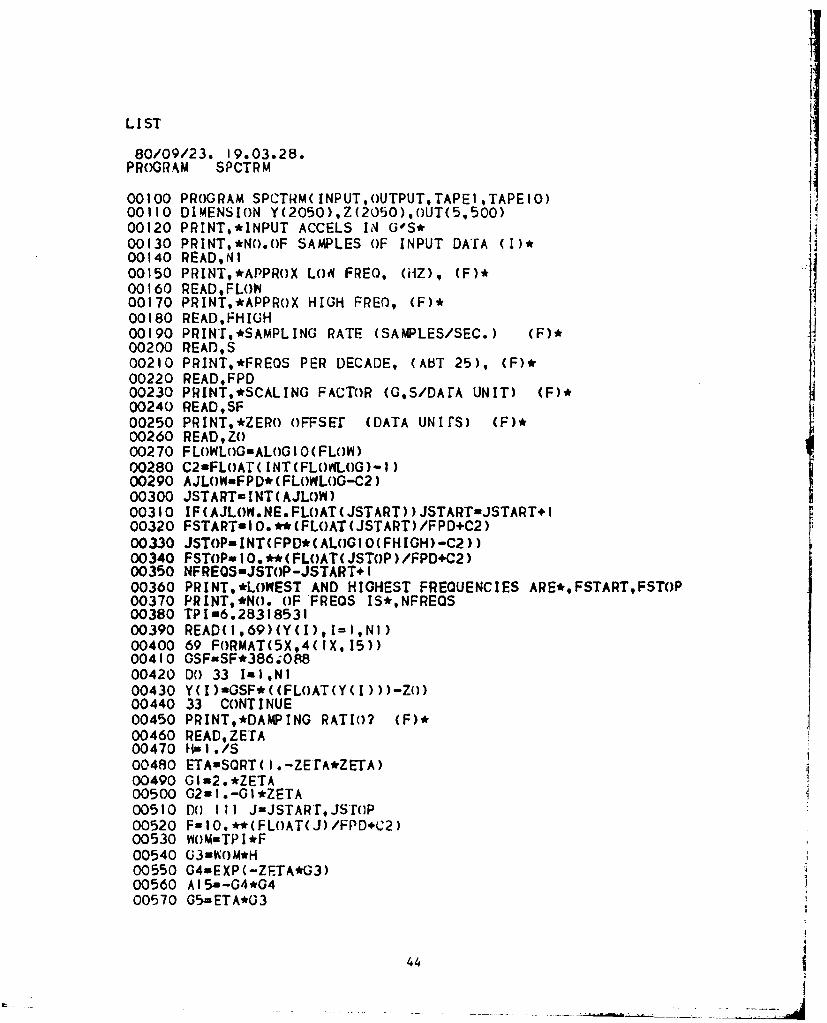
LIST

80/09/23. 19.03.28.PROGRAM SPCTRM

00100 PROGRAM SPCTRM( INPUT,OUTPUT.TAPEI,TAPEIO)00110 DIMENSION Y(2050),Z(2050).OUT(5.500)00120 PRINT,*INPUT ACCELS IN GOS*00130 PRINT,*NO.OF SAMPLES OF INPUT DATA (I*00140 READNI00150 PRINT,*APPROX LOAl FREO, OMlZ, (F)*00160 READIFLOW00170 PRINT,*APPROX HIGH FREO, (F)*00180 READ,FHIGH00190 PRINT,*SAMPLING RATE (SAMPLES/SEC.) (F)*00200 READ,S00210 PRINT,*FREOS PER DECADE, (ALIT 25), (F)*00220 READFPD00230 PRINT,*SCALING FACTOR (G,S/DArA UNIT) (F)*00240 READ,SF00250 PRINT,*ZER() OFFSET (DATA UNIfS) (F)*00260 READZO00270 FLOWLOG-ALOGI OCFLOW)00280 C2=FLOAr( INT(FU~wfLOG)-l)00290 AJL()WnFPD*(CFLOWLOG-C2)00300 JSTART- INT(CAJLOW)00310 IF(AJLOW.NE.FLOAT(JSTART) )JSTART=JSTART+I00320 FSTART.I0.**CFLOAT(JSTART)/FPD+C2)00330 JSTOPaINT(FPD*(ALOGIO(FH[GH)-C2))00340 FSTOP. 100 **(CFLOAT(CJSTOP )/FPD4C2)00350 NFREOS-JSTOP-JSTART. 100360 PRINT,*L()WEST AND HIGHEST FREQUENCIES ARE*,FSTART,FSTOP00370 PRINT,*NO. OF FREOS IS*,NFREOS00380 TPIm6.2831853100390 READ(1,69)(Y(I),I=I,NI)00400 69 FORMAT(5X,4(IX, 15))00410 GSF-SF*386;0~800420 Do) 33 IaI,NI00430 Y(I)nGSF*((FLOAT(Y(I)))-ZO)00440 33 CONTINUE00450 PRINT.*DAMPING RATIO? (F)*00460 READ,ZETA00470 11-1./S00480 ETAuSORT ( I .-ZErA*ZETA)00490 G1=2.*ZETA00500 02=1 .- G1*ZETA00510 Do IlIl J-JSTARTr,isT(Jp00520 F-tO. **(FLOAT(J)/FPD+C2)00530 W()M.TPI*F00540 03WKOM*H00550 04=EXP(-ZPTA*G3)00560 Al5.u-G4*0400570 G5=ETA*03

44

00580 G6-G4/ETA*S IN (05)*00590 CHI-G4*COS(G5)

00600 GJ-CHI/G600610 G8=-Al5/G600620 Al6a2.*CHI00630 All=-W~OM*0800640 Al 2=VOM*(G7-ZETA)00650 G9-O3*WOM00660 010-01+0300670 011*02*0600680 012009*PfOM

*00690 A24f(GI*CHI*At5*010+Gll)/012*00700 A25a2./G12*(03*CHI-GII-ZETA*(I..A15))*00710 A26.(GII+0I*(I.-CHI)-G3)/G12*00720 A27a(O;I*07-GB*010.02)/09

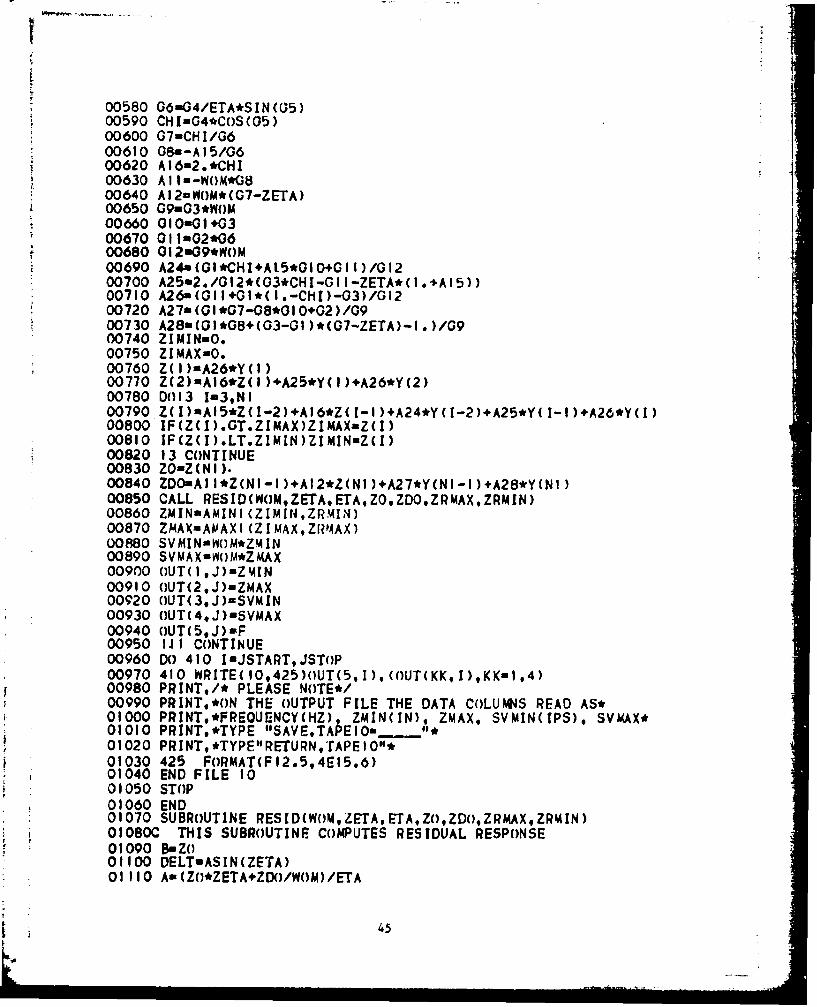
00130 A28u(0I*GB+(G3-GI)*C01-ZETA)-I.)/0900740 ZIMIN=.000750 ZIMAX-0.00760 Z(I)aA26*Y(i)00770 ZC2)=A)6*Z( I)+A25*Y( I)+A26*Y(2)00780 D013 1=31,NI00790 ZCI)aAI5*Z(1-2)+AI6*Z([-1lA24*Y(I-2s.A25*YU1-1l+A26*YcI)00800 IF(Z(I).GT.ZIMAX)ZIMAXnZ(I)00810 IF(Z(f).LT.ZIMIN)ZIMINuZ(I)00820 13 CONTINUE00830 ZO.ZCNI).00840 ZDO=AII*Z(N1-1)+AI2*Z(NI)+A27*Y(NI-l)+A28*Y(NI)00850 CALL RESID(WOMZETA,ETA.ZO,ZDO,ZRMAX,ZRMIN)00860 ZMINmAMIN1 (ZIMIrI,ZRMIN)00870 ZMA(AmAAAX I (Z IMAX tZIPAAX)00880 SVMiINaHOM*ZM4IN00890 SVMAX-oWM*ZMAX00900 OUT(1,J)=ZMIN00910 OUT(2.J)=ZMAX00920 OUT(3,J)=SVMIN00930 OUT(4,J)=SVMAX00940 OUT(5.J)&F00950 IJI CONTINUE00960 Do 410 ImJSTARTJSTOP00970 410 WRITE(10,425)OUT(5,I),,(OUT(KK,I),KK=1,4)00980 PRINT,/* PLEASE NOTE*/00990 PRINT,*ON THE OUTPUT FILE THE DATA COLUMNS READ AS*01000 PRINT,*FREQUENCYCHZ) ZMIN(IN), ZMAX, SVMIN(IPS). SVMAX*01010 PRINT.*TYPE "SAVE,TAh'EIO-.....*01020 PRINT,*TYPE"0RETURN.-TAPEI0"*01030 425 FORMAT(FI2.5,4E15.6)01040 END FILE 1001050 STOP

*01060 END01070 SUBROUTINE RES[D(WiOM,ZETA.ETA,ZO,ZDO,ZRMAXZRk~lN)01080C THIS SUBROUTINE COMPUTES RESIDUAL RESPONSE01090 BE ZO01100 DELT-ASIN(ZETA)

*01110 A=(ZO*ZETA.ZDO/WOM)/ETA

45

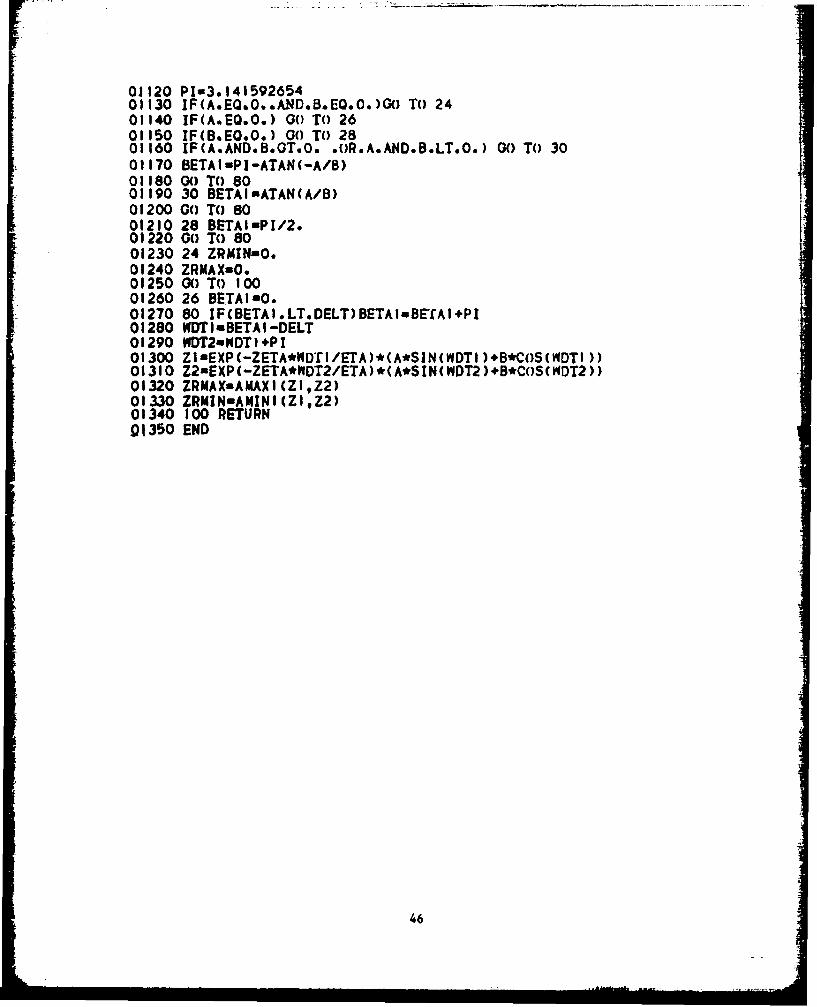
0J120 Plw3*14159265401130 IF(A.EQ.0..A!4D.B.EQ.o.)G0 To 2401140 IF(AoEQ.0.) GO TO 2601150 IF(B.EQ.0.) 00 TO 2801160 IF(A.AND.B.OT.0. .OR.A.AN4D.B.LT.0.) GO) TO) 3001170 BETAImPI-ATAN(-A/B)01180 00 TO) 8001190 30 BETAI-ATAN(A/B)01200 00 To 8001210 28 BETAI-PI/2.01220 00 To) 8001230 24 ZRMIN-0.01240 ZRMAX=O.01250 00) TO 10001260 26 BETAIuO.01270 80 IF(BETAI.LT.OELT)BETAI.DETAI+PI01280 WDTImBETAI-DELT01290 WDT2mWDT1I+PI101300 ZiUEXP(-ZETA*WDT1/ErA)*A*SIN(WDT,).B*COS(WDTI)01310 Z2nEXP(-ZETA*WDT2/ETA)*(A*SIN(IWDT2 )+B*COSO'fDT2))01320 ZRMAXmAMAXICZIZ2)01330 ZRMINuAMINICZI,Z2)01340 100 RETURN01350 END

46

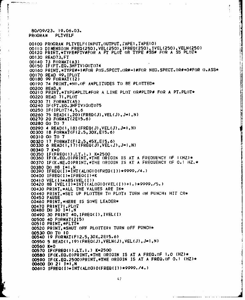
80/09/23. 19,06.03.PROGRAM PLTVELF

00100 PROGRAM PLTVELF( INPUT,OUTPUT,?;APEI ,TAPE1O)00110 DIMENSION FREO(250),VEL(250),IFREO(250), IVEL(250),VELN(250)

00120 PRINT,*TYPE#FTV#FoR A FT PLOT OR TYPE OSS# FOR A SS PLOT* 100130 RA73 FRATA300150 73(F.O.3HFTV)GT100160 PIN(T, TYEQ.3 I FT)OR T SETOR- FRNG.SET R40FROAS00160 PREAD 9,*YE+#o IPLOTTO#I#O E.SETOR+#OROA00180 9ED 9 PRMAT( 200190 74 PORINT,*OOFAPITDSTOB LOT

009 4PRINT,*TYPO.TLFR AMLINUEST BE.. RPTP ,APTPLOTTED

00200 READ N00220 PREAD 71,PLOPTL# A LINEPLOT ORPT0FORAP.lT00230 71A FORMAOTA500240 71(FT.O.3HTVA)G005100250 IF(IPLEO.HTV)4,5,6002607 F(PEAD(I),20(RE()VE(),100270 20 FCRMAT(1201.)(ROJEJ)-1N00280 20 TORMT27 S600290 4o TEoI,8(RE()VLJ7JI00300 18 FRMATC,1)FR2.5,30,VE15.6).J00300 18 TORMT 7 .,3XE5600320 17 ToRT(15 75 1560033061 FREADCT7(FR2 5(45XE15.),uIN00330 7 KEAOC,7(ROJ!E%)J1N00350 7FFE()L.. K=25000360 IFCK.EQ~)L.0RINTTH KRGN-2ATAFEQECY00lH)00370 IF(K.NEO.)PRINT,*THE ORIGIN IS AT A FREQUENCY oF 0.1HZ.*00380 DoKN-)PIT*H OR8I IS NTAFEUNY F01H.00390 DFRo(I)ulNT(LGOFE()*99/.00400 IFREO(I)-IFRE(AOI).K O~)*99./.00400 VFEL(I)uABS(ELCI))K00420 8IVEL(I)INTS(VE(Al))OVLI)I.*99/00430 88RINTLL -ITHE ALUES AREL IN*.*99./.00440 PRINT,*SELTH UPALOTES RE TOPOINTR*N UC; I00450 PAUTSETUPLTEToPo TRONUCHHIC*00460 PAUS,*ERISSELAE*00470 PRINT7IER 15SOLOEAER00480 DC) 30 IuIN00490 DO30 PIwlNT4,FE(IIEL00500 40 PORMAT(215)E~lIEL0050010 PORINT(2PLTT00510 PRINT,*SHUT OFPOrE;TR OFPN00530 0(1 To*HU OF10 ~ElTUNOFPNH00540 09 TORMTF1103X2E560055051 FRMAD(T9(FRE5,0(J,VELN(J),VLJfIN00560 5(ED 119-0OJVL()VL()J IN00570 IFFEQI.T.. K2000580 IFCK.EQ~)L.0PINTTH KRGI=S2TA5R00) 10(H00590 IF(K.EQ.250)PRINT,*THE ORIGIN IS AT A FREQ.OF 10. (HZ)*

00600 Do) 21 JIs,N00610 IFREQCI)sINTCAL()CIO(FREQ(I))*9999./4.)

47

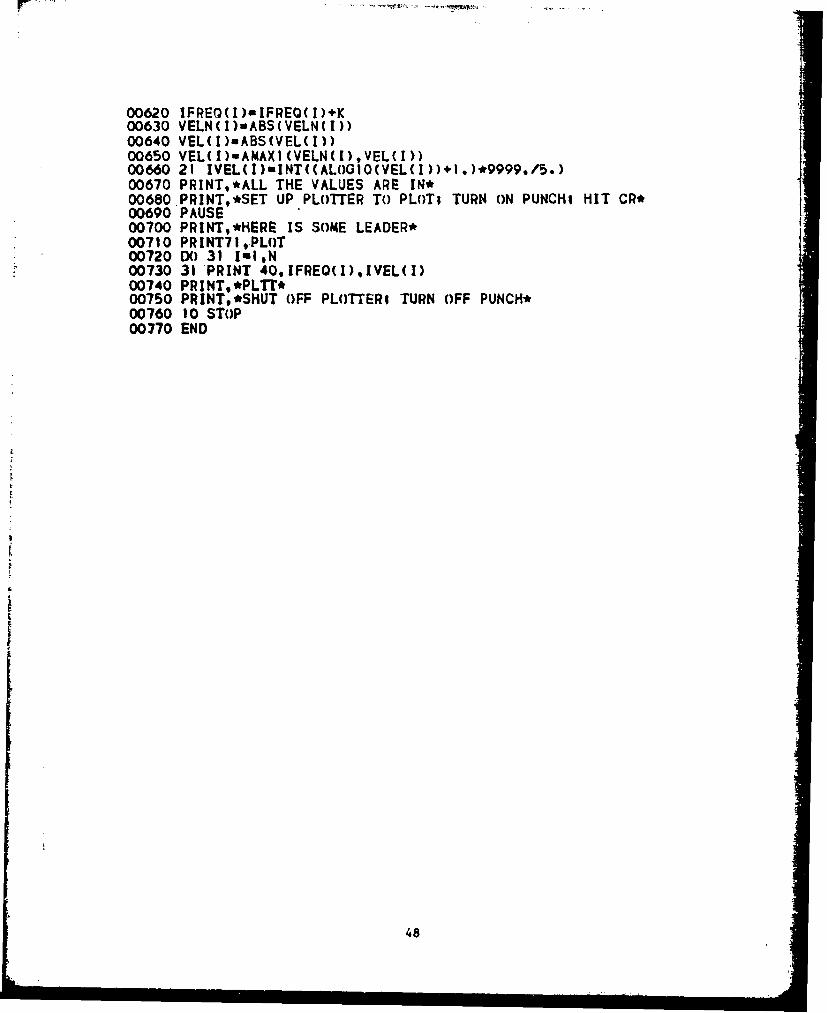
00620 IFREG(I)aIFREQCI)+K00630 VELNCI)=ABS(VELN(I))00640 VEL(I)aABS(VEL(I))00650 VEL(I)-AMAXICVELN(I),VEL(I))00660 21 IVEL(I)mINT(CALOGIO(VEL(I))+I.)*9999./5.)00670 PRINTs*ALL THE VALUES ARE IN*j00680 PRINT,*SET UP PLOTTER To PLOT; TURN ON PUNCH; HIT CR*00690 PAUSE I00700 PRINT,*IIERE IS SOME LEADER*00710 PRINT711-PLOT00720 Do) 31 IsIgN00730 31*PRINT 40, IFREO(I)IIVEL(I)00740 PRINT,*PLTr*00750 PRINT,*SHUT OFF PLOTTER; TURN OFF PUNCH*00160 10 STOP00770 END

48

Appendix C

DETAILS OF THE RESIDUAL SPECTRUM CALCULATION

The table given in the main text is repeated below to organize the

examination of the nine cases

A >0 A =0 A< 0

B > 0 I II 111

B = 0 IV V VI

B < 0 VII VIII IX

Because many values of A will satisfy Equation 15Sa, one imagines the

signs of A and B in Equation 15 to deduce the proper value of P for P1.

Case I, A > 0, B > 0

Consider a sketch of A cos P and B sin P as shown in Figure C-i.

Figure C-i.

As can be seen, PI is an acute angle, with tangent defined by Equation iSs,

and using principal angle notation

49

Tan- (A/B) (C-i)

Recall that (wdt) must be greater than zero; thus, from Equation 14, the

following check is made

- 06 ( 0 C-2)

If Condition C-2 is not fulfilled, the value of 1 must be increased by

n. The value of 02 is given by Equation 16 in all cases.

Case II, A = 0, B > 0

Consider Figure C-2.

B~5sin • A0

A ctI

Figure C-2.

In every case

0 (C-3)

However, in every case with damping, this value of will not satisfy

Condition C-2; thus,

0 n, if o (C-4)

Again 02 will be given by Equation 16.

50

di

il

Case III, A < 0, B > 0 PConsider the sketch of Figure C-3.

2

Figure C-3.

Clearly P1 is between n/2 aaid n, but note that if the negative of A cos

3 is drawn dotted, an angle p3 can be defined as

T= an' 1 (-A/B) (C-5)

The angle J is then given by (n - Oj) or

P =n - Tan- (-A/B) (C-6)

Condition C-2 would again be used to see if P, should be increased by R,

and Equation 16 would give 02 "

Case IV, A > 0, B = 0

Consider the sketch of Figure C-4.

Figure C-4.

51

Clearly R/ ff2. Condition C-2 would be checked, and Equation 16 used

for

Case V, A =0, B =0

Going back to the definition of A and B in Equations Ila and lib,

one sees that both z and ° are zero. Hence, no residual response

results, and both zmin and zmax are zero.

Case VI, A < 0, B = 0

Consider the sketch of Figure C-5.

Figure C-5.

Clearly P, = n/2. Condition C-2 would be checked, and Equation 16 used

for P

Case VII, B < 0, A > 0

Consider the sketch of Figure C-6.

AB-0 sin B sin

Figure C-6.

52

In this case P1 lies between n/2 and n. If the negative of B is used,

the acute angle •' can be obtained and subtracted from n as indicated

below.

S' = Tau (A/-B) (C-7a)

p1 = n - (C-7b)

Case VIII, A = 0, B < 0

Consider this situation drawn in Figure C-7.

• IA co, 4

Figure C-7.

As in Case II,

= 0 (C-8a)

but again in every case with damping, this value of P will not satisfy ICondition C-2; thus,

0 = i, if = 0 (C-8b)

As in all, cases 02 is given by Equation 16.

53

- - - - - 5- - -- - -!-

Case IX, A < 0 B < 0

Consider the sketch drawn in Figure C-8.

A Cos• P , a $ in 0

Figure C-8.

This use is the inverse of Case I, and I will always be acute and given

simply by

01 = Tan-1 (A/B) (C-9)

If Condition C-2 is not fulfilled, the value of el from Equation C-9

must be increased by n; the value of P2 is obtained from Equation 16.

That completes the examination of the nine possible cases identified

in Table 1. By going through them, one can organize the results as

follows.

Case V: A = B = 0,

no residual response occurs

Cases I, IX; A > 0, B > 0; or A < 0, B < 0,

0 = Tan' (A/B)

Cases III, VII: A < 0, B > 0; or B 0 0, A > 0,

01 = n- Tan- 1 (-A/B)

Cases II, VIII: A = 0, B > 0; or A = 0, B < 0,

=0

54

Cases IV, VI: A > 0, B 0 0; or A < 0, B : 0,

01 2

Now this suary can be organized into a more concise set of rules for

Sdetermination as follows:

1. If both A and B are zero, no residual response results.

2. If not, and A = 0, 01 = 0.

3. If not, and B = 0, PI = n/2.

4. If not, and A and B have the same sign,

= Tan" 1 (A/B)

5. If not,

= n - Tan- 1 (-A/B) .

Now given a value of PI. one applies Condition C-2, or if

P1 - 6 < 0

01 = (Piold + n

which yields acceptable values of I from which (wdt), can be obtained

with Equation 14 as follows

(wdt)l = P1 - 6 (C-10)

The second value of (wdt) is obtained from Equation 16 and is

(wdt) 2 = (Wdt)l + n

55

- 'i

I

Appendix D

FREQUENCY GENERATION FOR EQUALLY SPACED VALUES

WHEN PLOTTED ON LOGARITHMIC PAPER

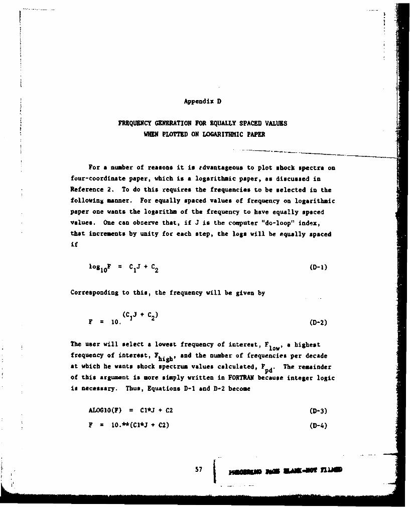
For a number of reasons it is tdvsntageous to plot shock spectra on

four-coordinate paper, which is a logarithmic paper, as discussed in

Reference 2. To do this requires the frequencies to be selected in the

following manner. For equally spaced values of frequency on logarithmic

paper one wants the logarithm of the frequency to have equally spaced

values. One can obeerve that, if J is the computer "do-loop" index,

that increments by unity for each step, the loss will be equally spaced

if

lo81 0 F = C1 J + C2 (D-1)

Corresponding to this, the frequency will be given by

F C 10. 1 2) (D-2)

The user will select a lowest frequency of interest, Flow' a highest

frequency of interest, Fhigh' and the number of frequencies per decade

at which he wants shock spectrum values calculated, F pd The remainder

of this argument is more simply written in FORTRAN because integer logic

is necessary. Thus, Equations D-1 and D-2 become

ALOGlO(F) = C1*J + C2 (D-3)

F lO.*(Cl*J + C2) (D-4)

57 m lkK-mw nu

Each time the log of the frequency increases by unity, the frequency

will have increased by a factor of 10, or gone through a decade; thus,

Cl is the recip&!al of Fpd' and Equations D-3 and D-4 may be written

ALOGIO(F) = J/TFF) + C2 (D-5)

F = 10.**(J/FPD + C2) (D-6)

Now, rather than start and stop at the precise low and high frequencies

selected by the user, one will start at FSTARI and stop at FSTOP, defined

z--be--he frequencies computed by Equation D-6 from the values of J

given as JSTART and JSTOP. Using functional notation this can be i2di-

cated by saying

FSTOP = F(JSTOP) (D-7)

FSTART = F(JSTART) (D-8)

The variables JSTOP and JSTART are defined such that

F(JSTART - 1) .LT. FLOW .LE. F(JSTART) (D-9)

and

F(JSTOP) .LE. FHIGH .LT. F(JSTOP + 1) (D-10)

This is convenient because the user will in general select an FPD, an

FLOW, and an FIHGH that are not mutually consistent. In this way, if

the user selects integer values of FPD, it is convenient to arrange C2

so that frequency values divisible by 10 are always included in the list

selected.In Equation D-S, C2 is an integer used so that J does not have to

assume zero or negative values. Whenever the starting frequency is less

than unity, the log of F will be negative. If C2 is one less than the

characteristic of the log of FSTART, J will always have to be greater

than zero. Thus, define:

58

C2 INT(ALOGIO(FLOW))- I (D-11)

To formulate a procedure to find JSTART, proceed as follows.

Substitute Equation D-6 into Condition D-9; take the log of all three

terms, which yields

(JSTART - 1)/FPD + C2 .LT. JLOW/FPD + C2 .LE.

(JSTART/FPD + C2) (D-12a)

Subtract C2 from each group, and then multiply through by the positive

number FPD which will yield

JSTART - I .LT. JLOW .LE. JSTART (D-12b)

where JSTART is an integer and JLOW is floating point and formed from

Equation D-5 with F equal to FLOW or

JLOW = FPD*(ALOGIO(FLOW) - C2) (D-13)

In general, JLOW will not have integral value; for the case where JLOW

is not integral

JSTART = INT(JLOW) + 1 (D-14)

but when JLOW does have integral value

JSTART = INT(JLOW) (D-15)

This can be programed as follows

FLOWLOG aALOG 10(FLOW)

C2 = FLOAT(INT(FLOWLOG) - 1)

AJ = FPD*(FLOWLOG - C2)

59

"6-

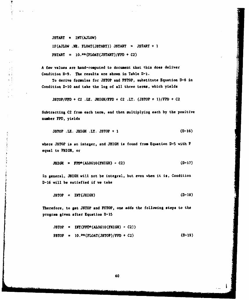
JSTART = INT(AJLOW)

IF(AJLOW .ME. FLOAT(JSTART)) JSTART = JSTART + 1

FSTART = 10.**(FLOAT(JSTART)/FPD + C2)

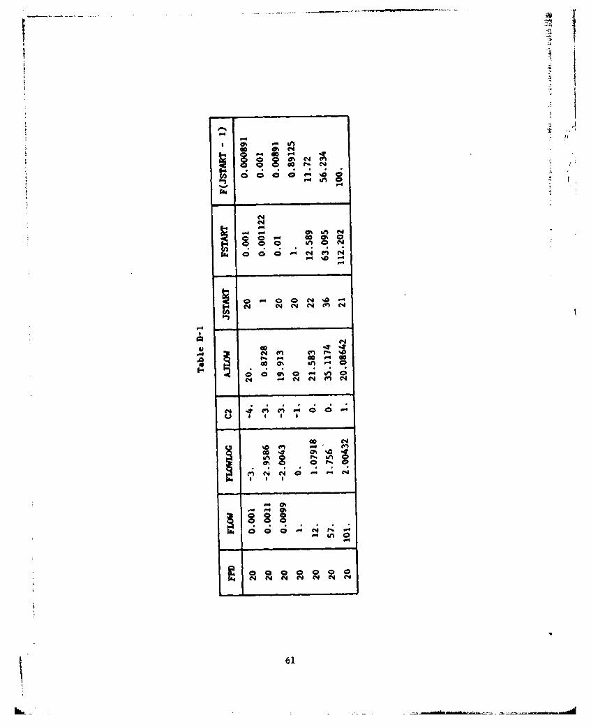
A few values are hand-computed to document that this does deliver

Condition D-9. The results are shown in Table D-1.

To derive formulas for JSTOP and ?STOP, substitute Equation D-6 in

Condition D-10 and take the log of all three terms, which yields

JSTOP/FPD + C2 .LE. JHIGN/FPD + C2 .LT. (JSTOP + 1)/FPD + C2

Subtracting C2 from each term, and then multiplying each by the positive

number FPD, yields

JSTOP .LE. J3il0G .LT. JSTOP + I (D-16)

where JSTOP is an integer, and JHIOH is found from Equation D-5 with F

equal to FMIGH, or

JHGII = FPD*(ALOGIO(FHIGH) - C2) (D-17)

In general, JHIGH will not be integral, but even when it is, Condition

D-16 will be satisfied if we take

JSTOP = INT(1IGH) CD-18)

Therefore, to get JSTOP &nd FnTOP, one adds the following steps to the

program given after Equation D-15

JSTOP INT(FPD*(ALOGO1(FHIGH) - C2))

,STOP - 10.**(FLOAT(JSTOP)/FPD + C2) (D-19)

60

I... ,

"94

coZ0Ne *

Go 01 G

S N C4 C N C4 C

p..1

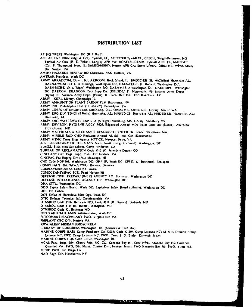
DISTRIBUTION LIST

AF Ho1 PREES Washington DC (R P Reid)AFB AF Tech Office (Mgt & Ops). Tyndall, Ft.; AFCECIXR,Tyndall FL-. CESCH, Wright-Patterson; HO

Tactical Air Cmd (R. E. Fisher), Langley AF13 VA; HQAFESCfDEMM. Tyndall AFB, FL; MACVDET(Col. P. Thompson) Scott, IL; SAMSOIMNNI). Norton AFB CA; Stinlo Library. Offurt NE; WPNS SafetyDiv, Norton, CA

AMMO HAZARDS REVIEW BD Chairman, NAS. Norfolk, VAAMTRAK President, Wash DCARMY ARRADCOM, Dover, NJ; ARRCOM, Rock Island, IL; BMDSC-RE (Ii. McClellan) Huntsville AL; 1

DAEN-CWE-M (LT C D Dinning). Washington DC; DAEN-FEU-E (). Ronan), Washington DC;DAEN-MCE.D (R L Wight) Washington DC; DAEN.MPE-D Washington DC; DAEN-MPU. WashingtonDC; DARCOM; ERADCOM Tech Supp Dir. (DELSD-L) Ft. Monmouth, NJ; Savanna Army Depot(Bynd). IL; Savanna Army Depot (Ernst). IL; Tech. Ref. Div.. Fort Huachuca, AZ

ARMY - CERL Library. Champaign ILARMY AMMUNITON PLANT SARHW-FEM Hawthorne, NVARMY COE Philadelphia Dist. (LIBRARY) Philadelphia, PAARMY CORPS OF ENGINEERS MRD-Eng. Div.. Omaha NE; Seattle Dist. Library. Seattle WAARMY ENG DIV ED-CS (S.Bolin) Huntsville. AL; HNDE-D-CS. Huntsv.ille AL-. HNDED-SR, Huntsville, AL;

Huntsville, ALARMY ENO WATERWAYS EXP STA (S Kiger) Vicksburg, MS; Library, Vicksburg MSARMY ENVIRON. HYGIENE AGCY B620, Edgewood Arsenal MD; Water Qual Div (Doner). Aberdeen

Prov Ground. MDARMY MATERIALS & MECHANICS RESEARCH CENTER Dr. Lenoc. Watertown MAARMY MISSILE R&D CMD Redstone Arsenal AL Sci. Info. Cen (Documents)ARMY MTMC Trans Engg Agency MTT.CE, Newport News, VAASST SECRETARY OF THE NAVY Spec. Assist Energy (Leonard). Washington, DCBUMED Field Med Svc School, Camp Pendleton. CABUREAU OF RECLAMATION Code 1512 (C. Selander) Denver COCINCLANT Civil Engr. Supp. Plans. Ofr Norfolk, VACINCPAC Fac Engrng Div (J44) Makalapa, HICNO Code NOP-964. Washington DC; OP-4I1F, Wash DC; 0P98IJ (J. Boosman). PentagonCOMFLEACIT. OKINAWA PWO, Kadena. OkinawaCOMNAVMARIANAS Code N4, GuamCOMOCEANSYSPAC SCE. Pearl Harbor HIDEFENSE CIVIL PREPARCiDNESS AGENCY JO0. Buchanan. Washington DCDEFENSE INTELLIGENCE AGENCY Dir.. Washington DCDNA STrL. Washington DCDOD Explos Safety board. Wash DC; Explosives Safety Board (Library). Washington DCDOE Dr. CohenDOT Office of Hazardous Mail Ops, Wash DCDTIC Defertse Technical Info CtrlAlextandria. VADTNSRDC` Code 1706. Bethesda MD; Code 41ll (it. Gierich), Bethesda MDDTNSRDC Code 4121 (R. Rivern), Annapolis. MDDTNSRDC Code 42, Bethesda MDFED RAILROAD AMIN Administrator. Wash DCFLTCOMBAJTR~ACENLANT PWO. Virginia Bch VAFMFLANT CEC Of~r. Norfolk VAKCWAJALEIN MISRAN BMDSC-RKL.CLIBRARY OF CONGRESS Washington. DC (Sciences & Tech Div)MARINE CORPS BASE Camp Pendleton CA 92055; Code 43.2ff0. Camp Lejeune NC;, M &R Division. Camp

Lejeune NC, PWO Camp Lejeune NC; PWO, Camp S. D. Butler. Kawasaki JapanMARINE CORPS 1105 Code LFF.2, Washington DCMCAS F661i. Engr. Div. Cherry Point NC; CO. Kaneohe Bay HI; Code PWE. Kaneohe Bay HI; Code S4.

Quantico VA;. PWD. Dir. Maint. Control Div., Iwakuni Japan; PWO Kaneohe Bay HI; PWO. Yuma AZMCRD PWO. San Diego CaNAD Engr. Dir. Hawthorne. NV

62

NAF PWD. Engr Div. Atsugi, Japan; PWO Sigonella Sicily; PWO. Atsugi Japan

NARF Code 100. Cherry Point, NC, Code 640, Pensacola FLNAS CO. Guantanamto Bay Cuba; Code 114. Alameda CA; Code 183 (Fac. Plan BR MGR); Code 187.

Jacksonville FL; Code 18700, Brunswick ME; Code 18U (ENS P.J. Hickey), Corpus Christi TX; Code 6234(G. Trask), Point Musgu CA; Code 70, Atlanta. Marietta GA; Dir. Util. Div.. Bermuda; ENS Buchholz,Pensacola. FL; Lakehurst, NJ; PW (J. Maguire), Corpus Christi TX; PWD Maint. Div., New Orleans, BelleChasse LA; PWD, Maintenance Control Dir.. Bermuda; PWD, Willow Grove PA; PWO Belle Chasse, LA;PWO Chase Field Beeville, TX; PWO Key West FL;, PWO Whiting FId, Milton FL-. PWO. Dallas TX;PWO, Glenview IL; PWO, Kingsville TX; PWO. Millington TN; PWO, Miramar, San Diego CA; PWO..Moffett Field CA; SCIE Lent Fleet Norfolk, VA; SCE Norfolk, VA. Security Offr. Alameda CA

NATL RESEARCH COUNCIL Naval Studies Board. Washington DCNATNAVMEDCEN PWO Bethesda. MDNAVACT PWO. London UK

* NAVAEROSPREGMEDCEN SCE, Pensacola FLNAVAIRSTA Code 500, San Diego. CANAVAIRSYSCOM PMA 258 Washington, DC

* ~NAVAVIONICFAC PWD Deputy Dir. DJ7OI, Indianapolis, INNAVCOASTSYSTCTR Code 423 (D. Good), Panama City FL; Code 713 (J. Quirk) Panama City. FL; Library

Panama City, FLNAVCOMMAREAMSTRSTA Code W-W0, Honolulu. Wahiawa HI; PWO. Norfolk VA, PWO. Wah:.awa HI;(1 SCE Unit I Naples ItalyNAVCOMMSTA CO (61E) Puerto Rico; CO, San Miguel. R.P.; Code 401 Nea Makri, Greece; PWO,

T Exmouth. Australia; PWO, Fort Amador Canal ZoneNAVEDTRAPRODEVCEN Tech. LibraryNAVEDUTRACEN Engr Dept (Code 42) Newport, RINAVEODFAC Code 605, Indian Head MDNAVFAC PWO, Brawdy Wales UK; PWO, Cape Hatteras, Buxton NC; PWO. Centerville Bch. Ferndale CA;

PWO. GuamNAVFAC PWO, Lewes DENAVPACENGCOM Code 043 Alexandria. VA; Code 044 Alexandria, VA; Code 0451 Alexandria, VA; Code

0454B Alexandria. Va; Code 0483 Alexandria, VA; Code 0405 Alexandria. VA: Code 100 Alexandr'ia, VA;

I Code 1113 (M. Carr) Alexandria. VA;. Code 1113 (T. Stevens) Alexandria, VA; Code 1113 Alexandria. VA;Morrison Yap, Caroline Is.; P W Brewer Alexandria, VA

N AVFACENGCOM - CHES DIV. Code 101 Wash. DC; Code 403 (H. DeVoe) Wash. DC; Code 405 Wash.DC; Code FPO- I Wash, DC11 NAVEACENGCOM -LANT DIV. CDR E. Peltier; Code I1l, Norfolk, VA; Eur. BR Deputy Dir. Naples Italy;European Branch. New York; RDT&ELO 102, Norfolk VA

NAVFACENGCOM -NORTH DIV. CO; Code 1028. RDT&ELO. Philadelphia PA; Code IIl (Castranovo)If Philadelphia, PA; Code 114 (A. Rhoads); Design Div. (R. Masino), 'hiladelphia PA; ROICC. Contracts.

NAVFACENGiCOM -PAC DIV. (Kyi) Code 101. Pearl Harbor. HI; Code 2011 Pearl Harbor. HI; Code 402.I RDT&E, Pearl Harbor HI; Commander. Pearl Harbor. HINAVFACENGCOM .SOUTH DIV. Code 09 (Watts) Charleston. SC; Code 90. RDT&ELO. Charleston SCNAVFACENGCOM .WEST DIV. 102; 112; AROICC. Contracts. Twentynine Palms CA; Code tl4B San

Bruno. CA; Code 402 San Bruno, CA; 09P/20 San Bruno, CA; RDT&ELO Code 2011 San Bruno, CANAVFACENGCOM CONTRACT AROICC, Point Mugu CA; AROICC, Quantico, VA. Code 05. TRIDENT.

Bremerton WA; D)ir. Eng. Div.. Exmouth. Australia; Eng Div dir. Southwest rac. Manila. PI; 01CC.Southwest Pac. Manila. PI; OICC/ROICC. Balboa Canal Zone; ROICC AF Guam; ROICC LANT DI'V..Norfolk VA; ROICC. Keflavik, Iceland;, ROICC. Pacific. San Bruno CA

NAVMAG SCE, GuamNAVNUPWRU MUSE DET Code NPU-30t Port Hueneme. CANAVOCEANSYSCEN Code 41. San Diego. CA; Code 67W0, Son Diego, CA; Research Lib.. San Dicgo CA;

Tech. Library, Code 447NAVORDSTA PWO. Louisville KYNAVPETOFF Code 30. Alexandria VANAVPGSCOL Code 61WL (0. Wilson) Monterey CANAVPHIBASE CO. ACB 2 Norfolk, VA; Code S3T. Norfolk VA

63

NAVRADRECFAC PWO. Kami Scya JapanNAVREGMEDCEN Chief of Police, Camp Pendleton CA; Code 29, Env. Health Scrv. (Al Bryson) San Diego.

CA: PWO Newport RI; PWO Portsmouth. VA; SCE (D. Kaye); SCE San Diego, CA; SCE, CampPendleton CA; SCE. Guam; SCE. Oakland CA

NAVSCOLCECOFF C35 Port Hueneme. CA,. CO, Code C44A Porn Hueneme. CANAVSEASYSCOM Code 05M13 (Newhouse) Wash DC; Code 6212, Wash DC; SEAO04H, Wash DCNAVSEC Code 603.4 (Library), Washington DC

NAVSECCIRUACT PWO. Adak AK; PWO. Edzell Scotland; PWO. Pueno Rico; PWO, Torni Sta. OkinawaLNAVSHIPREPFAC SCE Subic BayNAVSHIPYD; Code 202.4. Long Beach CA; Code 202.5 (Library) Puget Sound. Bremerton WA; Code 380,

(Woodroff) Norfolk, Portsmouth, VA; Code 400, Puget Sound; Code 400.03 Long Reach, CA; Code 404 1(IT J. Riccia), Norfolk. Portsmouth VA; Code 410. Mare Is.. Vailejo CA; Code 440 Portsmouth NH; Code440. Norfolk; Code 440. Puget Sound, Bremerton WA; Code 450. Charleston SC: Code 453 (Util. Sups).Vallejo CA; L.D. Vivian;, Library. Portsmouth NH; PWD (Code 400). Philadelphia PA: PWO. Mare Is.:-.PWO. Puget Sound: SCE. Pearl Harbor HI: Tech Library. Vallejo, CA

NAVSTA CO Naval Station. Maypon FL; CO Roosevelt Roads P.R. Puerto Rico; Dir Mcch Engr. Citmo;Engr. Dir.. Rota Spain; Long Beach, CA; Maint. Cont. Div., Guantanamo Bay Cuba; Maint. Div. Dir/Code531, Rodman Canal Zone; PWD (LTJG.P.M. Motolenich). Puerto Rico; PWO Midway Island; PWO,Keflavik Iceland; PWO. Mayport FL; ROICC. Rota Spain; SCE, Guam; SCE. San Diego CA; SCE. SubicBay, R.P.; Utilities Engr Off. (A.S. Ritchie), Rota Spain

NAVSUBASE ENS S. Dove. Groton, CT; SCE. Pearl Harbor HINAVSUPPACT CO. Seattle WA; Code 'ý. 12 Marine Corps Dist. Treasure It.. San Francisco CA; Code 413.

Seattle WA-: LTJG McGarrah. SEC. Vallejo, CA: Plan/fEngr Div., Naples ItalyNAVSURFWPNCEN PWO. White Oak. Silver Spring. MDNAVTECKTRACEN SCE. Pensacola FLNAVWPNCEN Code 2636 (W. Bonnet). China Lake CA: Code 3276 China Lake, CA; PWO (Code 26). China

Lake CA. ROICC (Code 702). Chini Lake CANAVWPNSTA (Clebak) Colts Neck, NJ: Code 09. C~oncord. CA: Code 092, Colib Neck NJ: Code 092A (C.

Frederick%) Seal Beach CA; Maint. Control Dir.. Yorktown VA; Naval Weapons Handling Center. Earle.NJ

NAVWPNSTA PW Office (Code 09C1) Yorkto%%r. VANAVWPNSTA Safety Br. Concord, CA; Security Offr, Colts Neck NJNAVWPNSUPPCEN Code 09 Crane INNCBU 405 OIC, San Diego, CANCBC Code 10 Davisville, RI; Code 155, Port Hucneme CA: Code 156, Port H-ueneme. CA: Code 400.

Gulfport MS; PW Engrg, Gulfport MIS: PWO (Codc 9ut) Port Iluenemne. CA; PWO, Dav~sville RINCBU 411 OIC, Norfolk VANCR 20. CommanderNCSO BAHRAIN Security Ofir. BahrainNMCB 5. Operations Dept.: 74. CO: Forty, CO: THREL. Operaiiions Off.NORDA Code 440 fOcet Rsch Off) IBav St Louis MSNRL Codc 844) Wabhington. DC; Code 8441 (ft A. Skop). Washington DCNSC Code 54.1 (Wynne). Norfolk VANSD SCE. Subic Bay. R.P.NTC Commander Orlando. FLNTSB Chairman, Wash DCNUSC Code 131 New London. CT: Code EA12.1 (R.S. Munn), New London Cl'OCEANSYSLANT LT A.R. Giancola. Norfolk VAOFFICE SECRETARY OF DEFENSE OASD (MRA&l.) Pentagon jL Cashcrgl. Wishington. D)CONR Code 7OOP Arlington VAPHIBCB I P&E. Coronado. CAPMTC Pat. Counsel. Point Mugu CAPWC (L~t E.S. Agonoy) Pensacola, rt.: ACE Office (LIJG St. Gecrmain) Noffolk V'A. (C Norfolk, VA: CO.

(Code 10). Oakland. CA: CO. Gireat Lakes IL:; Code lM. Great Lakes. It., ('ode 12,1, Oakland ('A. CodcI2IKX" (Library) San Diego. CA: Code 129, Guam,. Code 154. Oreat Lakes. It,: Code 2WK. Oteat L.i~kc- IL-:Code 220 Oakland. CA. ('ode 2'2ý1). INorfolk VA; Code 30tC. San Diego, CA, Code 4M*, Great Lakes. IL:.Code 400. Oakland. CA; Code 4M8. Pcarl Harbor. HI; Code 4M.1 San Diego. CA: ('ode 42(1) Great Lakes.IL: Code 420. Oakland. C~A; Code 42B (R. Pascua). Pearl Harbor HI. Code 5f05A (if Wheeler); Code (00,

64

Great Lakes. IL; Code 601. Oakland, CA: Code 610, San Diego Ca; Code 700. Great Lakes, IL; Code 700,San Diego. CA; LTJG J.L. McClaine, Yokosuka, Japan; Utilities Officer, Guam; XO (Code 20) Oakland,CA

SPCC PWO (Code 120) Mechanicsburg PANAF PWO (Code 30) El Centro, CAU.S. MERCHANT MARINE ACADEMY Kings Point. NY (Reprint Custodian)USCO (Smith). Washington, DC; G.EOE-4/61 (T. Dowd), Washington DCUSEUCOM (ECJ4JL-LO), Wright, Stuttgart. GEUSNA Ch. Mech. Engr. Dept Annapolis MD; PWD Engr. Div. (C. Bradford) Annapolis MDCALIFORNIA STATE UNIVERSITY LONG BEACH, CA (CHELAPATI)CORNELL UNIVERSITY Ithaca NY (Serials Dept, Engr Lib.)DAMES & MOORE LIBRARY LOS ANGELES. CAILLINOIS STATE GEO. SURVEY Urbana ILLEHIGH UNIVERSITY Bethlehem PA (Fritz Engr. Lab No. 13, Beedle); Bethlehem PA (Linderman Lib.

No.30. Flecksteiner)MICHIGAN TECHNOLOJICAL UNIVERSITY Houghton, MI (Haas)MIT Cambridge MA; Cambridge MA (Rm 10-500, Tech. Reports. Engr. Lib.): Cambridge MA (Whitman)NEW MEXICO SOLAR ENERGY INST. Dr. Zwibel Las Cruces NMNY CITY COMMUNITY COLLEGE BROOKLYN. NY (LIBRARY)PURDUE UNIVERSITY Lafayette, IN (CE Engr. Lib)CONNECTICUT Hartford CT (Dept of Plan. & Energy Policy)SEATTLE U Prof Schwaegler Seattle WASOUTHWEST RSCH INST R. DeHart, San Antonio TXSTANFORD UNIVERSITY Engr Lib. Stanford CASTATE UNIV- OF NEW YORK Buffalo, NY

"TEXAS A&M UNIVERSITY W.B. Ledbetter College Station. TXUNIVERSITY OF CALIFORNIA BERKELEY. CA (CE DEPT, GERWICK); Berkeley CA (E. Pearson).

DAVIS, CA (CE DEPT. TAYLOR)- LIVERMORE, CA (LAWRENCE LIVERMORE LAB, TOKARZ)UNIVERSITY OF DELAWARE Newark. DE (Dept of Civil Engineering. Chesson)UNIVERSITY OF HAWAII Honolulu HI (Dr. Szilard)UNIVERSITY OF ILLINOIS Metz Ref Rm, Urbana IL; URBANA. IL (LIBRARY); URBANA, IL

(NEWMARK): Urbana IL (CE Dept, W. Gamble)UNIVERSITY OF MASSACHUSETTS (Heronemus), Amherst MA CE DeptUNIVERSITY OF MICHIGAN Ann Arbor MI (Richart)UNIVERSITY OF NEBRASKA-LINCOLN Lincoln. NE (Ross Ice Shelf Proj.)UNIVERSITY OF NOTRE DAME Katona. Notre Dame. INUNIVERSITY OF TEXAS inst. Marine Sei (Library). Port Arkansas TXUNIVERSITY OF TEXAS AT AUSTIN AUSTIN. TX (THOMPSON); Austin, TX (Breen)UNIVERSITY OF WASHINGTON Dept of Civil Engr (Dr. Mattock). Seattle WA: SEATTLE. WA

(MERCHANT)UNIVERSITY OF WISCONSIN Milwaukee WI (Ctr of Great Lakes Studies)AMMAN & WHITNEY CONSULT ENGRS N Dobbs New York, NY

ARVID GRANI OLYMPIA. WAASSOC AMER RR Bureau of Explosive, Chicago. ILATLANTIC RICHFIELD CO DALLAS. TX (SMITH)AUSTRALIA Dept of Const. Canberra; Dept of Hsng & Const. SydneyBECHTEL CORP. SAN FRANCISCO. CA (PHELPS)

BROWN & CALDWELL E M Saunders Walnut Creek, CA 4CANADA Mem Univ Newfoundland (Chari). St Johns. Trans.Mni Oil Pipe Lone Corp. Vancouver, BC CanadaCOLUMBIA GULF TRANSMISSION CO. HOUSTON. TX (ENG. LIB.)HERCULES INC. D Richardson. Magna. UTDURLACH. O'NEAL, JENKINS & ASSOC. Columbia SCFORD. BACON & DAVIS, INC. New York (LibrarvyFRANCE Dr. Dutcrtre, BoulogneGLIDDEN CO. STRONGSVILLE. OH (RSCH LIB)

HUGHES AIRCRAFT Culver City CA (Tech. Doc. Ctr)ITALY M. Cai;oni. MilanKAMAN SCIENCES CORP T Cook Colorado Springs. CO

65

f-• I -- | 1 I I q I "

I

LOCKHEED MISSILES & SPACE CO. INC. Sunnyvale, CA (K.L. Krug)MCDONNEL AIRCRAFT CO. Dept 501 (RH. Fayman), St Louis MO; Navy Tech Rep S, Louis, MO; R

Carson, St. Louis, MONEWPORT NEWS SHIPBLDG & DRYDOCK CO. Newport News VA (Tech. Lib.)NORWAY DET NORSKE VERITAS (Library), Oslo; DET NORSKE VERITAS (Roren) iuslo; i. ross, Oslo;-

J. Creed, Ski; Norwegian Tcch Univ (Brandtzaeg), TrondheimPORTLAND CEMENT ASSOC. Skokie IL (Rich & Dav Lab, Lib.)RAND CORP. Santa Monica CA (A. Laupa)RAYMOND INTERNATIONAL INC. E Colle Soil Tech Dept. Pennsauken, NJSANDIA LABORATORIES Library Div.. Livermore CA; Seabed Progress Div 4536 (D. Talbert) Albuquerque

NMSCHUPACK ASSOC SO. NORWALK, CT (SCHUPACK)SHELL OIL CO. HOUSTON, TX (MARSHALL)SWEDEN Cement & Concrete Research Inst., Stockholm; GcoTech InstSWITZERLAND T Schneider, ZurichTHE NETHERLANDS Director Tech Rsch Prins Maurits Lab, Rijswijk

TRW SYSTEMS REDONDO BEACH, CA (DAI)UNITED KINGDOM Atomic Energy Auth (F R Farmer) London; Cement & Concrete Assoc Wexham Springs,

Slough Bucks; D. Lee. London; D. New, G. Maunsell & Partners, London; R. Browne, Southall.Middlesex; Taylor, Woodrow Constr (014P), Southall. Middlesex

WESTINGHOUSE ELECTRIC CORP. Annapolis MD (Oceanic Div Lib, Bryan); Library, Pittsburgh PAWESTINTRUCORP Egenon, Oxnard, CAWISS, JANNEY, ELSTNER, & ASSOC Northbrook, IL (D.W. Pfeifer)WOODWARD-CLYDE CONSULTANTS (A. Hamgan) San FranciscoBRAHTZ La Jolla, CABROWN, ROBERT University, ALBRYANT ROSE Johnson Div. UOP, Glendora CABULLOCK La CanadaF. HEUZE Alamo, CACAPT MURPHY Sunnyvale, CAR.F. BESIER Old Saybrook CTT.W. MERMEL Washington DC

66