Embed Size (px)
Citation preview

Game playing
Chapter 6
Chapter 6 1

Outline
♦ Games
♦ Perfect play– minimax decisions– α–β pruning
♦ Resource limits and approximate evaluation
♦ Games of chance
♦ Games of imperfect information
Chapter 6 2

Games vs. search problems
“Unpredictable” opponent ⇒ solution is a strategyspecifying a move for every possible opponent reply
Time limits ⇒ unlikely to find goal, must approximate
Plan of attack:
• Computer considers possible lines of play (Babbage, 1846)
• Algorithm for perfect play (Zermelo, 1912; Von Neumann, 1944)
• Finite horizon, approximate evaluation (Zuse, 1945; Wiener, 1948;Shannon, 1950)
• First chess program (Turing, 1951)
• Machine learning to improve evaluation accuracy (Samuel, 1952–57)
• Pruning to allow deeper search (McCarthy, 1956)
Chapter 6 3

Types of games
deterministic chance
perfect information
imperfect information
chess, checkers,go, othello
backgammonmonopoly
bridge, poker, scrabblenuclear war
battleships,blind tictactoe
Chapter 6 4
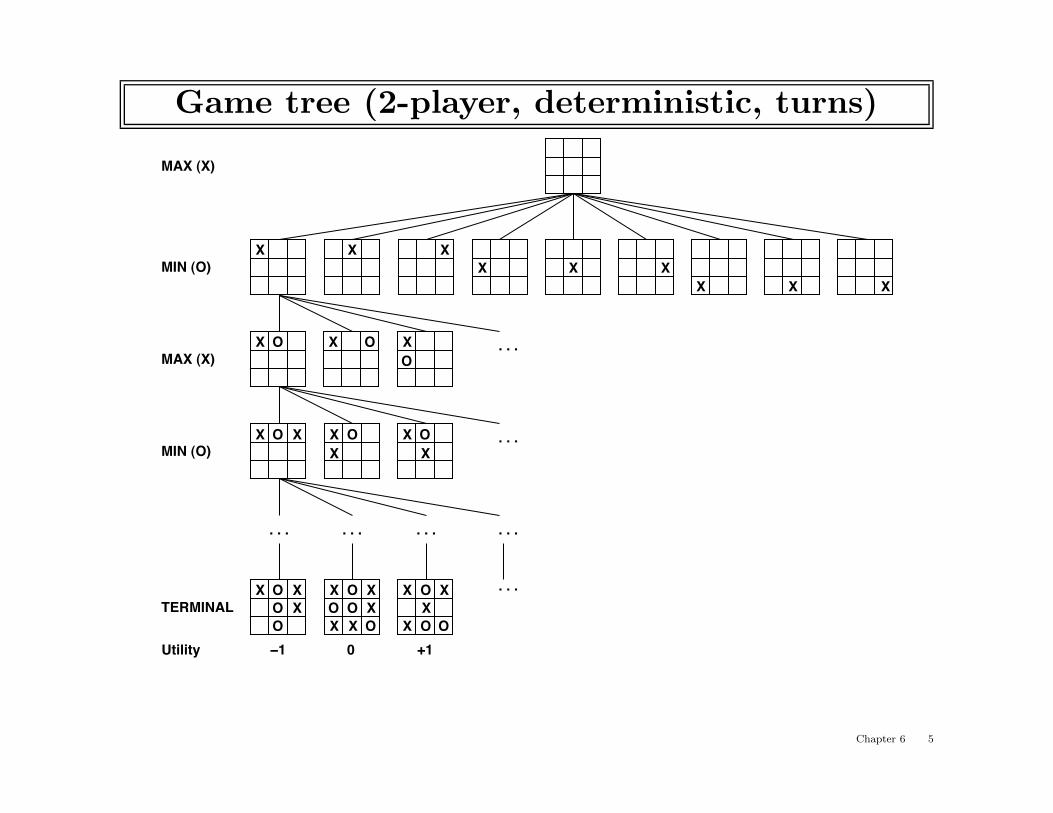
Game tree (2-player, deterministic, turns)
XXXX
XX
X
XX
MAX (X)
MIN (O)
X X
O
OOX O
OO O
O OO
MAX (X)
X OX OX O XX X
XX
X X
MIN (O)
X O X X O X X O X
. . . . . . . . . . . .
. . .
. . .
. . .TERMINAL
XX−1 0 +1Utility
Chapter 6 5
Minimax
Perfect play for deterministic, perfect-information games
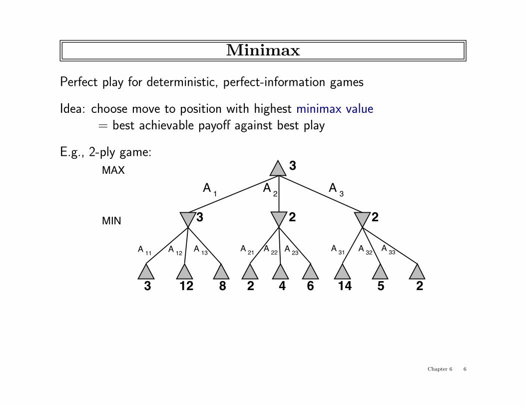
Idea: choose move to position with highest minimax value= best achievable payoff against best play
E.g., 2-ply game:MAX
3 12 8 642 14 5 2
MIN
3A 1 A 3A 2
A 13A 12A 11 A 21 A 23A 22 A 33A 32A 31
3 2 2
Chapter 6 6

Minimax algorithm
function Minimax-Decision(state) returns an actioninputs: state, current state in game
return the a in Actions(state) maximizing Min-Value(Result(a, state))
function Max-Value(state) returns a utility valueif Terminal-Test(state) then return Utility(state)v←−∞for a, s in Successors(state) do v←Max(v, Min-Value(s))return v
function Min-Value(state) returns a utility valueif Terminal-Test(state) then return Utility(state)v←∞for a, s in Successors(state) do v←Min(v, Max-Value(s))return v
Chapter 6 7
Properties of minimax
Complete??
Chapter 6 8
Properties of minimax
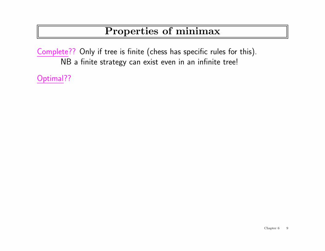
Complete?? Only if tree is finite (chess has specific rules for this).NB a finite strategy can exist even in an infinite tree!
Optimal??
Chapter 6 9
Properties of minimax
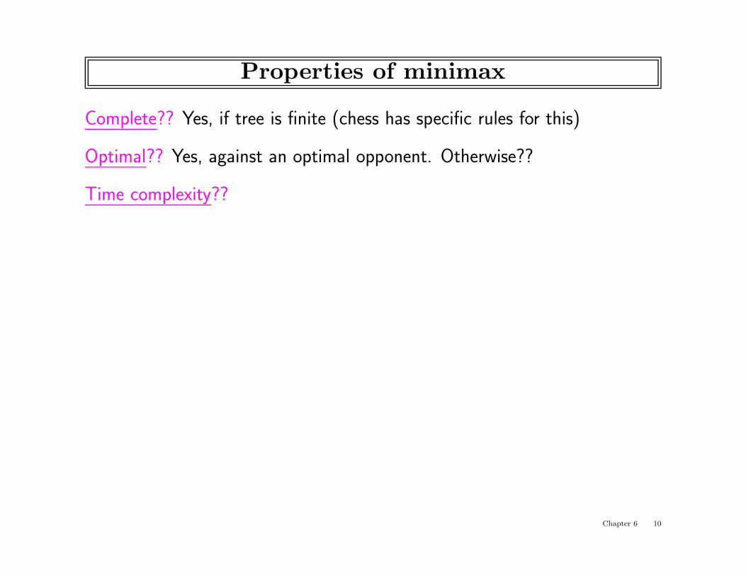
Complete?? Yes, if tree is finite (chess has specific rules for this)
Optimal?? Yes, against an optimal opponent. Otherwise??
Time complexity??
Chapter 6 10

Properties of minimax
Complete?? Yes, if tree is finite (chess has specific rules for this)
Optimal?? Yes, against an optimal opponent. Otherwise??
Time complexity?? O(bm)
Space complexity??
Chapter 6 11

Properties of minimax
Complete?? Yes, if tree is finite (chess has specific rules for this)
Optimal?? Yes, against an optimal opponent. Otherwise??
Time complexity?? O(bm)
Space complexity?? O(bm) (depth-first exploration)
For chess, b ≈ 35, m ≈ 100 for “reasonable” games⇒ exact solution completely infeasible
But do we need to explore every path?
Chapter 6 12

tlp • Spring03 • 9
USCF rating USCF rating
depth 1200
7 8 9 10 11 12 13 4 5 6
MacHack
World champ
2000 Expert
2900

α–β pruning example
MAX
3 12 8
MIN 3
3
Chapter 6 13

α–β pruning example
MAX
3 12 8
MIN 3
2
2
X X
3
Chapter 6 14
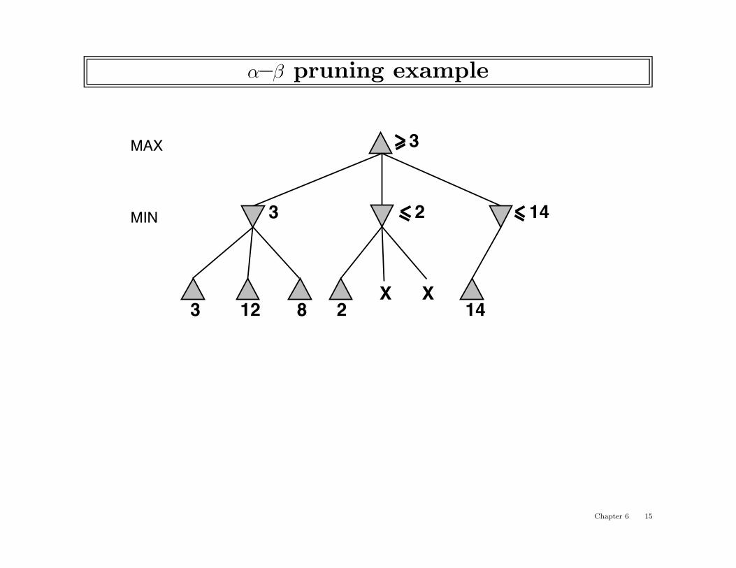
α–β pruning example
MAX
3 12 8
MIN 3
2
2
X X14
14
3
Chapter 6 15

α–β pruning example
MAX
3 12 8
MIN 3
2
2
X X14
14
5
5
3
Chapter 6 16
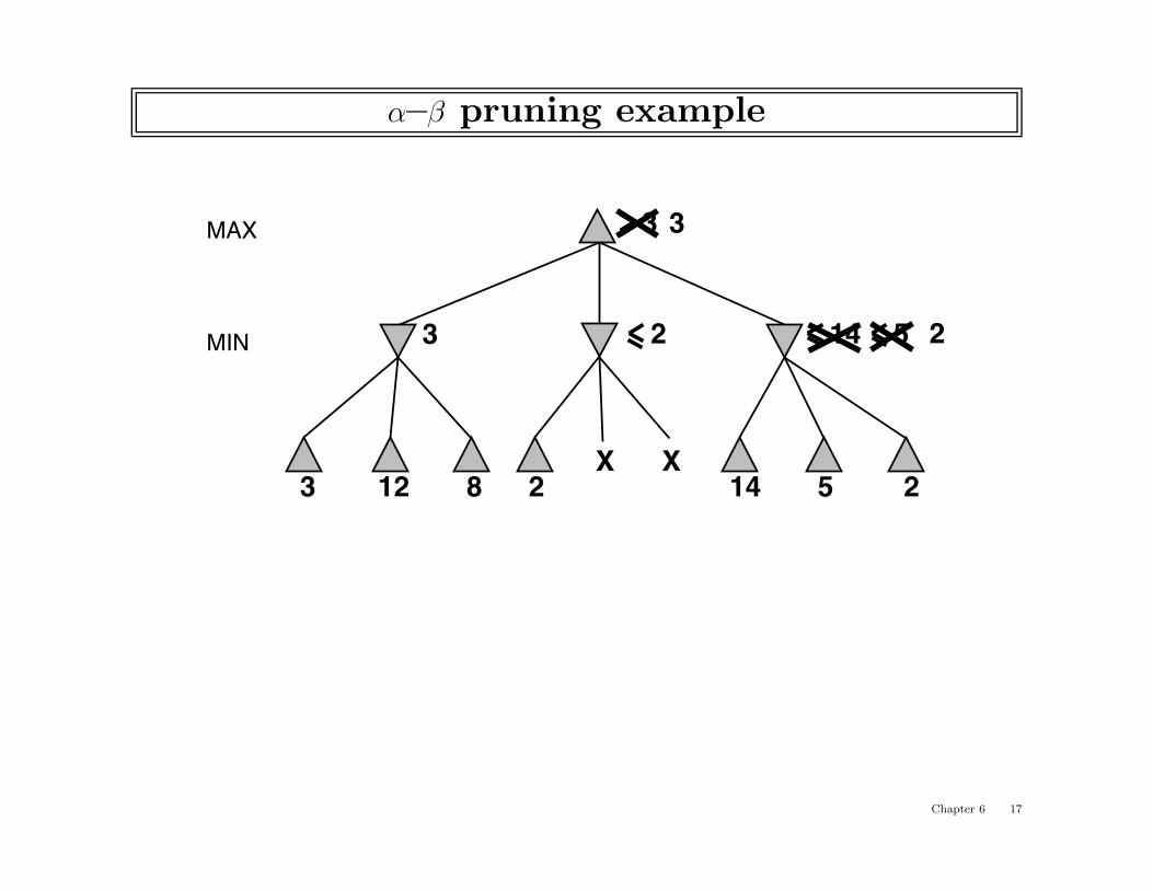
α–β pruning example
MAX
3 12 8
MIN
3
3
2
2
X X14
14
5
5
2
2
3
Chapter 6 17
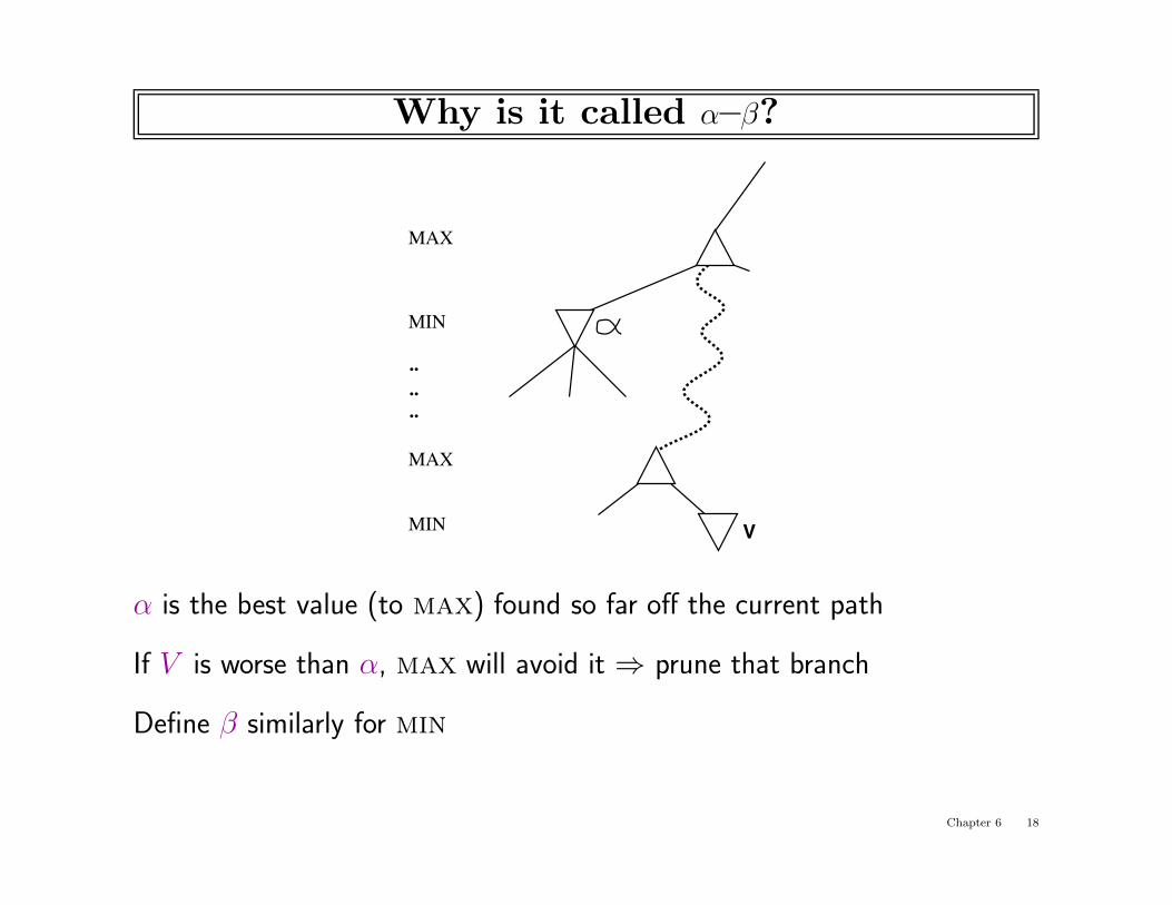
Why is it called α–β?
..
..
..
MAX
MIN
MAX
MIN V
α is the best value (to max) found so far off the current path
If V is worse than α, max will avoid it ⇒ prune that branch
Define β similarly for min
Chapter 6 18
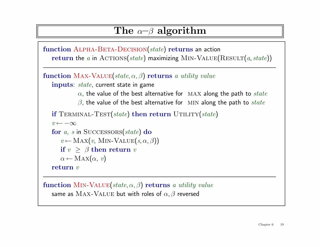
The α–β algorithm
function Alpha-Beta-Decision(state) returns an actionreturn the a in Actions(state) maximizing Min-Value(Result(a, state))
function Max-Value(state,α,β) returns a utility valueinputs: state, current state in game
α, the value of the best alternative for max along the path to stateβ, the value of the best alternative for min along the path to state
if Terminal-Test(state) then return Utility(state)v←−∞for a, s in Successors(state) do
v←Max(v, Min-Value(s,α,β))if v ≥ β then return vα←Max(α, v)
return v
function Min-Value(state,α,β) returns a utility valuesame as Max-Value but with roles of α,β reversed
Chapter 6 19
Properties of α–β
Pruning does not affect final result
Good move ordering improves effectiveness of pruning
With “perfect ordering,” time complexity = O(bm/2)⇒ doubles solvable depth
A simple example of the value of reasoning about which computations arerelevant (a form of metareasoning)
Unfortunately, 3550 is still impossible!
Chapter 6 20

Resource limits
Standard approach:
• Use Cutoff-Test instead of Terminal-Teste.g., depth limit (perhaps add quiescence search)
• Use Eval instead of Utilityi.e., evaluation function that estimates desirability of position
Suppose we have 100 seconds, explore 104 nodes/second⇒ 106 nodes per move ≈ 358/2
⇒ α–β reaches depth 8 ⇒ pretty good chess program
Chapter 6 21
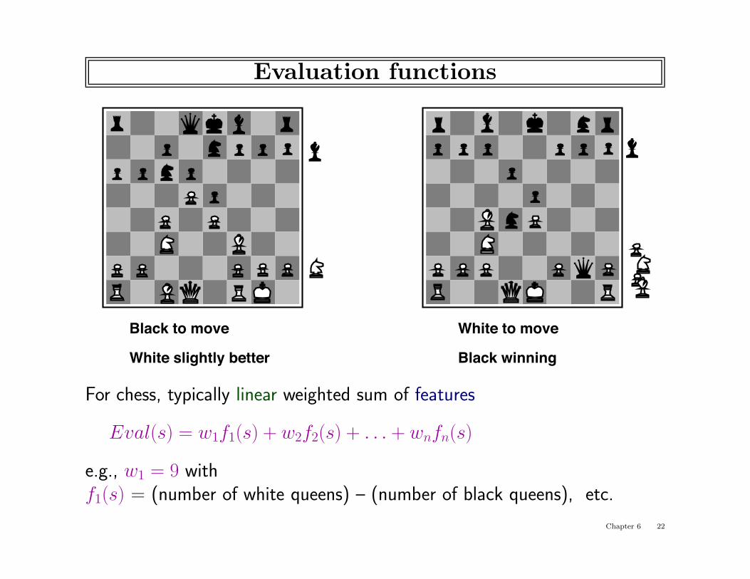
Evaluation functions
Black to move
White slightly better
White to move
Black winning
For chess, typically linear weighted sum of features
Eval(s) = w1f1(s) + w2f2(s) + . . . + wnfn(s)
e.g., w1 = 9 withf1(s) = (number of white queens) – (number of black queens), etc.
Chapter 6 22

Digression: Exact values don’t matter
MIN
MAX
21
1
42
2
20
1
1 40020
20
Behaviour is preserved under any monotonic transformation of Eval
Only the order matters:payoff in deterministic games acts as an ordinal utility function
Chapter 6 23

tlp • Spring03 • 28
Game Program
1. Move generator (ordered moves) Time 50%
2. Static evaluation 40% 3. Search control 10%
openings end games
databases
[ all in place by late 60’s.]
tlp • Spring03 • 29
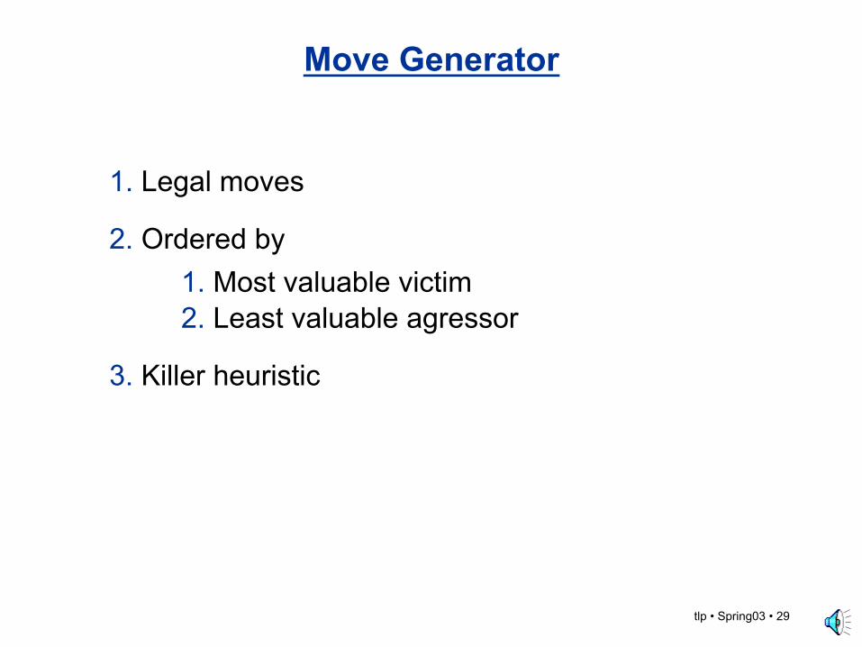
Move Generator
1. Legal moves
2. Ordered by 1. Most valuable victim 2. Least valuable agressor
3. Killer heuristic

tlp • Spring03 • 30
Static Evaluation
Deep searchers: moderately complex (hardware)
PC programs: elaborate, hand tuned
Very Complex
Very simple (material)
70’s -
Initially -
now -
tlp • Spring03 • 31
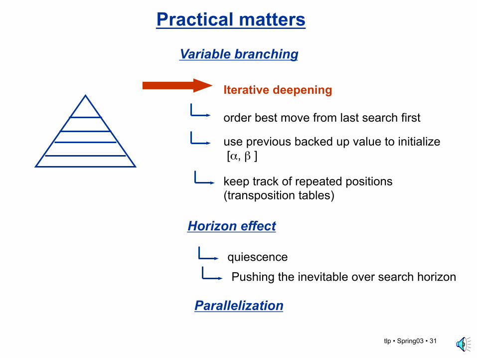
Practical matters
Iterative deepening
order best move from last search first
keep track of repeated positions (transposition tables)
use previous backed up value to initialize [#, ! ]
Variable branching
Horizon effect
Parallelization
quiescence
Pushing the inevitable over search horizon

Deterministic games in practice
Checkers: Chinook ended 40-year-reign of human world champion MarionTinsley in 1994. Used an endgame database defining perfect play for allpositions involving 8 or fewer pieces on the board, a total of 443,748,401,247positions.
Chess: Deep Blue defeated human world champion Gary Kasparov in a six-game match in 1997. Deep Blue searches 200 million positions per second,uses very sophisticated evaluation, and undisclosed methods for extendingsome lines of search up to 40 ply.
Othello: human champions refuse to compete against computers, who aretoo good.
Go: human champions refuse to compete against computers, who are toobad. In go, b > 300, so most programs use pattern knowledge bases tosuggest plausible moves.
Chapter 6 24

The Monte-Carlo Revolution in Go
Remi Coulom
Universite Charles de Gaulle, INRIA, CNRS, Lille, France
January, 2009
JFFoS’2008: Japanese-French Frontiers of Science Symposium
Introduction
Monte-Carlo Tree Search
History
Conclusion
Game Complexity
How can we deal with complexity ?
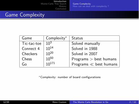
Game Complexity
Game Complexity∗ StatusTic-tac-toe 103 Solved manuallyConnect 4 1014 Solved in 1988Checkers 1020 Solved in 2007Chess 1050 Programs > best humansGo 10171 Programs � best humans
∗Complexity: number of board configurations
Remi Coulom The Monte Carlo Revolution in Go 2 / 12

Introduction
Monte-Carlo Tree Search
History
Conclusion
Game Complexity
How can we deal with complexity ?
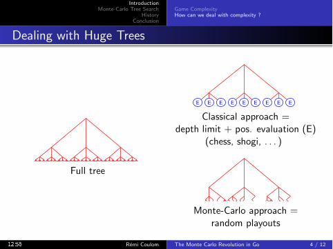
Dealing with Huge Trees
Full tree
E E E E E E E E E
Classical approach =depth limit + pos. evaluation (E)
(chess, shogi, . . . )
Monte-Carlo approach =random playouts
Remi Coulom The Monte Carlo Revolution in Go 4 / 12

Introduction
Monte-Carlo Tree Search
History
Conclusion
Game Complexity
How can we deal with complexity ?
Dealing with Huge Trees
Full tree
E E E E E E E E E
Classical approach =depth limit + pos. evaluation (E)
(chess, shogi, . . . )
Monte-Carlo approach =random playouts
Remi Coulom The Monte Carlo Revolution in Go 4 / 12
Introduction
Monte-Carlo Tree Search
History
Conclusion
Principle of Monte-Carlo Evaluation
Monte-Carlo Tree Search
Patterns
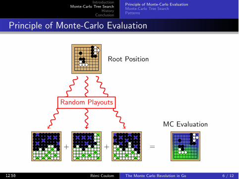
Principle of Monte-Carlo Evaluation
Root Position
MC Evaluation
+ + =
Random Playouts
Remi Coulom The Monte Carlo Revolution in Go 6 / 12
Introduction
Monte-Carlo Tree Search
History
Conclusion
Principle of Monte-Carlo Evaluation
Monte-Carlo Tree Search
Patterns
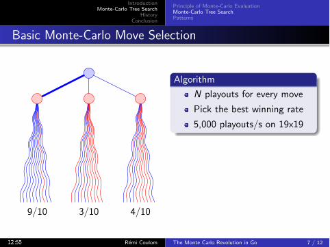
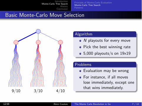
Basic Monte-Carlo Move Selection
4/103/109/10
Algorithm
N playouts for every move
Pick the best winning rate
5,000 playouts/s on 19x19
Problems
Evaluation may be wrong
For instance, if all moveslose immediately, except onethat wins immediately.
Remi Coulom The Monte Carlo Revolution in Go 7 / 12
Introduction
Monte-Carlo Tree Search
History
Conclusion
Principle of Monte-Carlo Evaluation
Monte-Carlo Tree Search
Patterns
Basic Monte-Carlo Move Selection
4/103/109/10
Algorithm
N playouts for every move
Pick the best winning rate
5,000 playouts/s on 19x19
Problems
Evaluation may be wrong
For instance, if all moveslose immediately, except onethat wins immediately.
Remi Coulom The Monte Carlo Revolution in Go 7 / 12

Introduction
Monte-Carlo Tree Search
History
Conclusion
Principle of Monte-Carlo Evaluation
Monte-Carlo Tree Search
Patterns
Monte-Carlo Tree Search
3/92/69/15
Principle
More playouts to bestmoves
Apply recursively
Under some simpleconditions: provenconvergence to optimalmove when#playouts→∞
Remi Coulom The Monte Carlo Revolution in Go 8 / 12
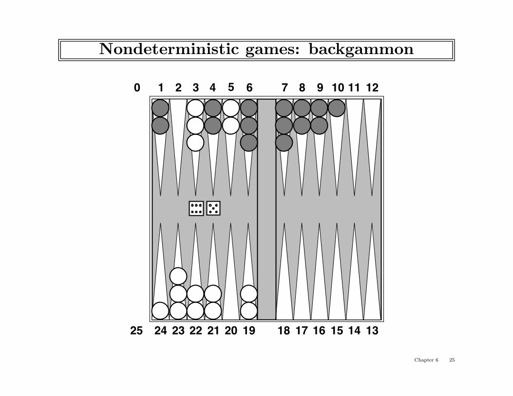
Nondeterministic games: backgammon
1 2 3 4 5 6 7 8 9 10 11 12
24 23 22 21 20 19 18 17 16 15 14 13
0
25
Chapter 6 25

Nondeterministic games in general
In nondeterministic games, chance introduced by dice, card-shuffling
Simplified example with coin-flipping:
MIN
MAX
2
CHANCE
4 7 4 6 0 5 −2
2 4 0 −2
0.5 0.5 0.5 0.5
3 −1
Chapter 6 26
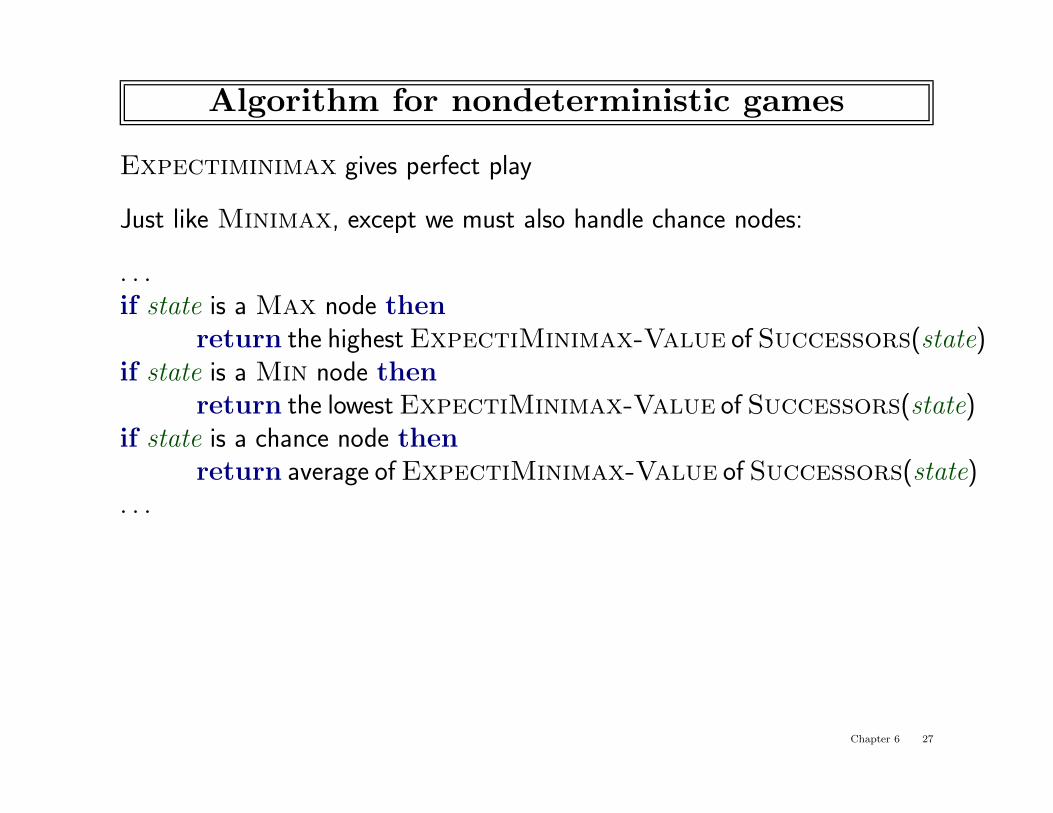
Algorithm for nondeterministic games
Expectiminimax gives perfect play
Just like Minimax, except we must also handle chance nodes:
. . .if state is a Max node then
return the highest ExpectiMinimax-Value of Successors(state)if state is a Min node then
return the lowest ExpectiMinimax-Value of Successors(state)if state is a chance node then
return average of ExpectiMinimax-Value of Successors(state). . .
Chapter 6 27
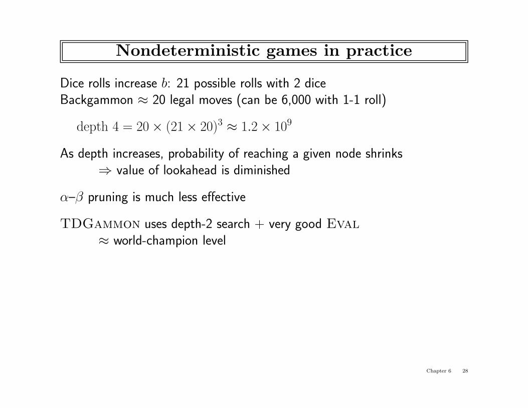
Nondeterministic games in practice
Dice rolls increase b: 21 possible rolls with 2 diceBackgammon ≈ 20 legal moves (can be 6,000 with 1-1 roll)
depth 4 = 20 × (21 × 20)3 ≈ 1.2 × 10⁹
As depth increases, probability of reaching a given node shrinks⇒ value of lookahead is diminished
α–β pruning is much less effective
TDGammon uses depth-2 search + very good Eval≈ world-champion level
Chapter 6 28
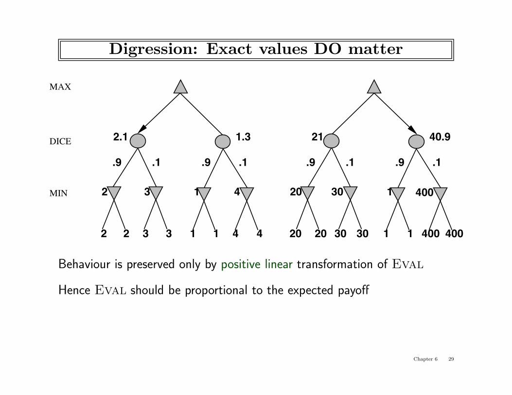
Digression: Exact values DO matter
DICE
MIN
MAX
2 2 3 3 1 1 4 4
2 3 1 4
.9 .1 .9 .1
2.1 1.3
20 20 30 30 1 1 400 400
20 30 1 400
.9 .1 .9 .1
21 40.9
Behaviour is preserved only by positive linear transformation of Eval
Hence Eval should be proportional to the expected payoff
Chapter 6 29

Games of imperfect information
E.g., card games, where opponent’s initial cards are unknown
Typically we can calculate a probability for each possible deal
Seems just like having one big dice roll at the beginning of the game∗
Idea: compute the minimax value of each action in each deal,then choose the action with highest expected value over all deals∗
Special case: if an action is optimal for all deals, it’s optimal.∗
GIB, current best bridge program, approximates this idea by1) generating 100 deals consistent with bidding information2) picking the action that wins most tricks on average
Chapter 6 30

Commonsense example
Road A leads to a small heap of gold piecesRoad B leads to a fork:
take the left fork and you’ll find a mound of jewels;take the right fork and you’ll be run over by a bus.
Chapter 6 34
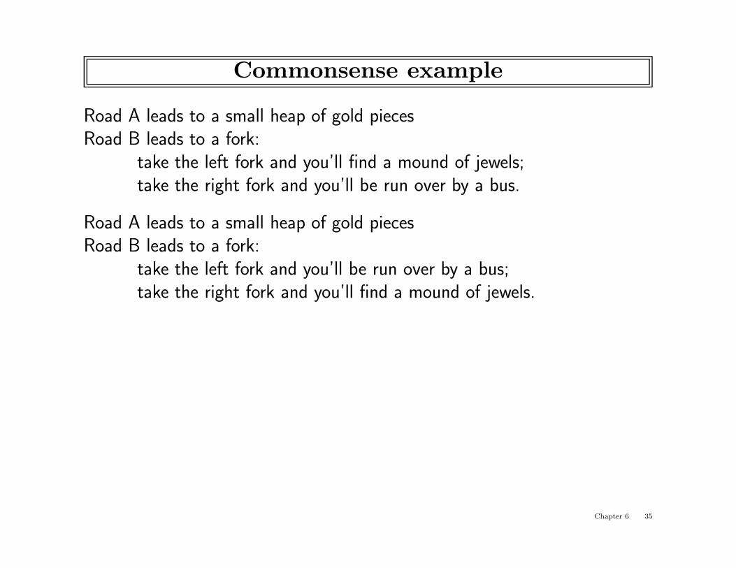
Commonsense example
Road A leads to a small heap of gold piecesRoad B leads to a fork:
take the left fork and you’ll find a mound of jewels;take the right fork and you’ll be run over by a bus.
Road A leads to a small heap of gold piecesRoad B leads to a fork:
take the left fork and you’ll be run over by a bus;take the right fork and you’ll find a mound of jewels.
Chapter 6 35

Commonsense example
Road A leads to a small heap of gold piecesRoad B leads to a fork:
take the left fork and you’ll find a mound of jewels;take the right fork and you’ll be run over by a bus.
Road A leads to a small heap of gold piecesRoad B leads to a fork:
take the left fork and you’ll be run over by a bus;take the right fork and you’ll find a mound of jewels.
Road A leads to a small heap of gold piecesRoad B leads to a fork:
guess correctly and you’ll find a mound of jewels;guess incorrectly and you’ll be run over by a bus.
Chapter 6 36
Proper analysis
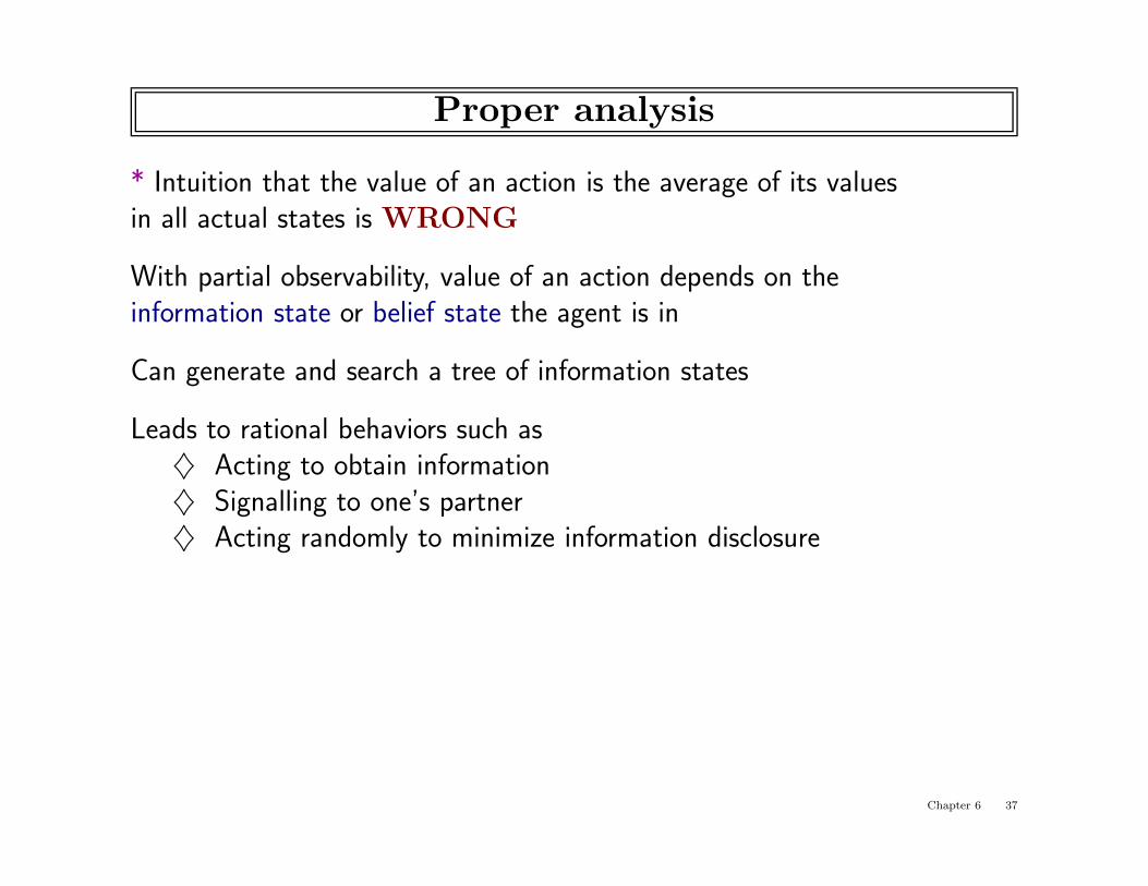
* Intuition that the value of an action is the average of its valuesin all actual states is WRONG
With partial observability, value of an action depends on theinformation state or belief state the agent is in
Can generate and search a tree of information states
Leads to rational behaviors such as♦ Acting to obtain information♦ Signalling to one’s partner♦ Acting randomly to minimize information disclosure
Chapter 6 37
Summary
Games are fun to work on! (and dangerous)
They illustrate several important points about AI
♦ perfection is unattainable ⇒ must approximate
♦ good idea to think about what to think about
♦ uncertainty constrains the assignment of values to states
♦ optimal decisions depend on information state, not real state
Games are to AI as grand prix racing is to automobile design
Chapter 6 38