Effective Field Theory

Joseph D. Roussos

Abstract

This essay is a review article on effective field theory. This is a technique inquantum field theory which allows for the construction of new theories from knownLagrangians; either ‘top-down’ (taking the known Lagrangian as the high-energytheory and deriving a low-energy effective theory) or ‘bottom-up’ (taking the knownLagrangian as the low-energy theory and incorporating it into an effective theoryapproximating an unknown high-energy theory). This article reviews the basics ofeffective field theory construction in each of these cases. The delivery is aimed at aMaster’s student with some knowledge of quantum field theory.

Contents

1 Introduction 3

2 Top-Down Construction of an EFT 42.1 A brief outline of the process . . . . . . . . . . . . . . . . . . . . . . . . . . 42.2 Integrating out . . . . . . . . . . . . . . . . . . . . . . . . . . . . . . . . . 5

2.2.1 Path integral formulation . . . . . . . . . . . . . . . . . . . . . . . . 52.2.2 Effective Lagrangian formulation . . . . . . . . . . . . . . . . . . . 6

2.3 Power counting . . . . . . . . . . . . . . . . . . . . . . . . . . . . . . . . . 72.3.1 Naıve dimensional analysis . . . . . . . . . . . . . . . . . . . . . . . 82.3.2 Scaling . . . . . . . . . . . . . . . . . . . . . . . . . . . . . . . . . . 82.3.3 Naturalness . . . . . . . . . . . . . . . . . . . . . . . . . . . . . . . 10

2.4 Tree-level matching . . . . . . . . . . . . . . . . . . . . . . . . . . . . . . . 102.5 Renormalisation . . . . . . . . . . . . . . . . . . . . . . . . . . . . . . . . . 13

2.5.1 Renormalisability and EFT . . . . . . . . . . . . . . . . . . . . . . 132.5.2 Renormalisation schemes and EFTs . . . . . . . . . . . . . . . . . . 142.5.3 Higher-order matching . . . . . . . . . . . . . . . . . . . . . . . . . 14

3 Bottom-Up EFTs and the PEW Measurements 163.1 Introduction . . . . . . . . . . . . . . . . . . . . . . . . . . . . . . . . . . . 163.2 Background . . . . . . . . . . . . . . . . . . . . . . . . . . . . . . . . . . . 17

3.2.1 Electroweak symmetry breaking . . . . . . . . . . . . . . . . . . . . 173.2.2 Custodial symmetry . . . . . . . . . . . . . . . . . . . . . . . . . . 183.2.3 Vacuum polarisation . . . . . . . . . . . . . . . . . . . . . . . . . . 183.2.4 Precision electroweak measurements . . . . . . . . . . . . . . . . . . 19

3.3 Effective operators . . . . . . . . . . . . . . . . . . . . . . . . . . . . . . . 213.3.1 The Peskin-Takeuchi parameters . . . . . . . . . . . . . . . . . . . 213.3.2 Oblique operators . . . . . . . . . . . . . . . . . . . . . . . . . . . . 22

3.4 Constraints on new physics . . . . . . . . . . . . . . . . . . . . . . . . . . . 22

4 Conclusion 24

Acknowledgements

I would like to thank Dr Daniel Baumann for his friendly advice and support in writingthis essay. I’m grateful to my friend Aaron Levy who, despite not studying advancedquantum field theory, listened sympathetically to my monologues on this essay.

1 Introduction

The effective theory approach is a technique in physics which exploits a simple but re-markably useful fact about nature: physical problems often come with distinct energyscales. The physical processes dominant at well-separated scales differ, and an effectivetheory focuses on the important physics in a manner which is conceptually clear andassists in calculations.

We are well acquainted with this idea, and frequently simplify physical problems by,for example, setting small masses to zero when they occur together with large masses. Weare able to do this because of the experimental fact that most of the details of low energyphysics are independent of the details of high energy physics. The history of physics tellsus it had to be this way, as otherwise we would have had no success in the Newtoniandomain without a proper understanding of particle physics. The aim of effective fieldtheory (EFT) is to rigorously apply this idea to field theory, excluding as much of thedetail of the high energy theory as possible when doing low energy physics. In order todo this we must ask two questions. First, which high energy features are important atlow energies? Second, which low energy processes are most sensitive to the details of highenergy physics? We can go some way toward answering this latter question even whenwe don’t know the high energy theory; a remarkable feature of this approach.

There are many motivations for using EFTs:

1. They simplify calculations. This is useful when we don’t want to waste time calcu-lating the details of unimportant high energy dynamics, or when we simply don’tknow those details.

2. They can parametrise additions to known physics. By constructing an EFT extend-ing our known theory, we can parametrise the impact on current observables due tonew physics.

3. They clarify the link between old and new physical theories. For example, EFTshows us how the Fermi theory of the weak interaction arises from full electroweaktheory and explains where and why it is accurate.

4. They explain why certain approximations are suspiciously accurate. EFT shows ushow to organise calculations of results which depend on deep symmetries, such asthe Quantum Hall effect, in a manner which explains why seemingly heavy-handedapproximations don’t compromise accuracy.

EFT has had a unique impact on quantum field theory, giving firm grounding to thephysics of renormalisation. The natural endpoint of the thinking that led from the originalad hoc “cancellation of infinities” to the renormalisation group equations is EFT. It givesnew meaning to the renormalisation group, and explains when and why renormalisabletheories arise. EFT also rehabilitates non-renormalisable theories, by showing how andwhy they can give accurate results.

Taking effective field theory seriously means accepting that all our theories are at besteffective theories of some higher, currently unknown, theories. They are all therefore onlyvalid up to some energy level. This doesn’t reduce their practical efficacy, as experimentscan only probe finite energy ranges. Problems may occur if we can probe outside the rangeof our current theory’s application. But this is simply a way of describing the businessof high energy physics: our theories of physics are necessarily responses to or inspired

3

by the experimental data available at a given energy range. We don’t know the highenergy theory of everything, so we design theories which fit energy scales accessible tous. We make predictions beyond the currently accessible energy range and then wait forexperimental corroboration/falsification as a new generation of experiments come on-line.

Not all of the above will be discussed in depth here. My focus is the constructionof EFTs, specifically in the context of a weakly interacting UV theory1. There are twocases: constructing an effective theory from a known high-energy theory and casting aknown theory as an effective theory in order to test the viability of new models. In section2, I will focus on the former, laying out a systematic method of deriving a low energyeffective theory from a known Lagrangian. In section 3 I will turn to an example of usingEFT methods to new physics, in a discussion on the use of precision electroweak (PEW)measurements in constraining physics beyond the Standard Model.

2 Top-Down Construction of an EFT

2.1 A brief outline of the process

In order to construct an effective field theory from a known high energy theory we adoptroughly the following process. First, we identify the relevant light fields (and their symme-tries) for the physical domain we want to study. Our aim is to exclude fields heavier thanthese from direct consideration. To do so we choose a cut-off energy level, and integrateout field modes with momenta above this level. In practice the exclusion of these fieldsinvolves writing down a general Lagrangian for the light fields, as a sum of all allowedoperators, with as yet unknown coefficients.

In general we will find that the higher the order of the operator, the smaller itscontribution to low energy physics. This allows us to truncate the sum in order to attainresults of a given accuracy. Since our aim is to match experimental results, which arealways of finite accuracy, this is sufficient to do physics. This process of determiningwhich operators we need to keep and which we can discard is called power counting. Itinvolves examining how the relative contributions of various local operators changes overthe energy range of the EFT.

Having accomplished this truncation we need to determine the values of the coeffi-cients. We decide on an observable to calculate, and perform the calculation in both thefull and effective theory. In the full theory, the calculation will involve an expansion inpowers of the heavy scale. We then match the coefficients in the effective theory equal tothose given by a specific order in the heavy scale expansion. In this way we incorporatethe heavy physics into the couplings of the effective theory in just such a manner as toreproduce the full theory observables to a given accuracy.

The effective theory we have now obtained is a new theory, with new interactions thatcan be treated perturbatively2 using Feynman graphs. Note, however, that renormalis-ability is not a criterion which constrains which operators are “allowed” in our effectiveLagrangian so there is no guarantee it is renormalisable. One important conceptual gainfrom the EFT approach is that we need not be worried by non-renormalisable terms:given that we’re only interested in a fixed level of precision, we can calculate in a non-renormalisable theory. Indeed, such terms will capture some important details of theunderlying high energy dynamics.

1I will make explicit note of where the method outlined here depends on the couplings being weak.2It is possible to construct non-perturbative EFTs, but I shall not consider them.

4

The new graphs we obtain are typically easier to compute than those of the full theorybecause they are local: we have exchanged graphs with heavy particle propagators forgraphs with local vertices. They are usually more divergent than those of the full theory,but still easier to handle as handling the finite parts of graphs is the most intensive portionof the calculation.

If we want to perform loop calculations in our EFT we will have to regulate andrenormalise our integrals as in ordinary QFT. Matching takes place order-by-order in aloop expansion, with the effective coefficients from the previous order included in thenext. There is some debate about how to renormalise in EFTs, which comes down to twodifferent conceptions of how to do effective field theory. This will be discussed in section2.5.

2.2 Integrating out

In this section I will describe the formalism of “integrating out” heavy modes from atheory3.

In order to make any headway, we first need to ask what we mean by “heavy”. Effectivetheories require the existence of a scale gap. Suppose our system has a characteristic scaleE0 and that we are interested in physics below this level. For example, in particle physics,we might not be interested in very heavy particles like the top quark. We choose a cut-offΛ which is smaller than E0. The heavy particles cannot be produced on-shell below Λ,and as this is as high as we will go when calculating, we will not consider them directly.

Having set the scale Λ we proceed to divide the field content φ of our theory intoheavy and light parts. Schematically, we split φ = φH + φL. Typically, the Lagrangianswe work with have light fields φ and heavy fields Φ, and so a natural first step is to write

L[φ,Φ] = Ll[φ] + Lh[Φ] + Llh[φ,Φ], (1)

where Ll (Lh) describes the part of L involving only the light (heavy) fields, and Llhincludes all interactions involving both fields. This does not imply, however, that it isenough to naıvely identify heavy and light fields in the Lagrangian.

There are now two descriptions of how we derive an effective action. In the first weliterally perform a path integral over all field modes heavier than the cut-off. In thesecond (which I will use) we write down an effective Lagrangian which applies below thecut-off, which does not include the heavy fields. I will briefly describe the formal integraland then demonstrate the construction of an effective Lagrangian.

2.2.1 Path integral formulation

The Wilson effective action4 is defined as

ei SW [φL] =

∫d[φH ]ei S[φL, φH ] (2)

Note that the field splitting described above requires some careful work. Given L[φ,Φ]with just two fields, and mφ �MΦ, it might be tempting to regard the task of generating

3This section draws from Polchinski [1] and three of Cliff Burgess’ lectures [2, 3, 4].4Named for Ken Wilson whose 1974 paper began the modern study of EFTs.

5

the Wilson effective action as that of choosing m < Λ < M and performing the pathintegral over Φ: ∫

d[Φ] ei S[φ,Φ].

However, we also need to take into account high frequency modes of φ. To see how thisworks, consider a mode expansion of the light field,

φ(x) =∑`

c`u`(x),

∫d4xu`(x)u`′(x) = δ``′ , (3)

where the basis functions u` are eigenfunctions of the differential operator ∆ that describesthe kinetic term in the action:

∆u` = ω`u`. (4)

These eigenvalues ω` give precise meaning to the idea of the frequency of the field. So ifwe write the full path integral as ∫

d[φ]d[Φ] ei S[φ,Φ],

then the light field measure is

d[φ] =∏`

dc`, (5)

and we can use equation (4) to define high energy modes as those with ω` > Λ and lowenergy as ω` < Λ. We split the measure

d[φ] =

∏`

ω`<Λ

dc`

∏

`ω`>Λ

dc`

≡ d[φ]l.e.d[φ]h.e.. (6)

The correct definition of the Wilson effective action is then

ei SW [φ] ≡∫

Λ

d[φ]h.e.d[Φ] ei S[φ,Φ]. (7)

Note that this integral is difficult to perform, and is often done in a perturbative expansionusing Feynman diagrams [5] or using a saddle-point approximation [6].

2.2.2 Effective Lagrangian formulation

One can derive an effective action without performing a path integral. Instead we writedown the most general thing which could be the desired effective Lagrangian, which isto say that we write an infinite sum of all operators involving the light fields whichare allowed by the symmetries of the full theory. As SW is an integral over high energymodes, the uncertainty principle guarantees that the remaining interactions must be local.Energies available in the effective theory are low, so high energy effects are produced bylocal violations of energy conservation. These are allowed only so long as they occur oververy small times. The same applies to momentum/distance.

The effective Lagrangian can thus be expanded as

Leff[φ] = Ll[φ] +∑i

giOi[φ]. (8)

6

with the Oi local. To see what these operators look like, consider an example. Take thefollowing Lagrangian,

L = −1

2∂µφ∂

µφ− 1

2∂µΦ∂µΦ− M2

2Φ2 − m2

2φ2 − V (φ,Φ), (9)

and choose m < Λ < M . Our effective Lagrangian will include only φ and be valid only upto Λ. We can organise our expansion of Leff in powers of derivative terms5. The originalLagrangian was invariant under φ→ −φ so we will preserve that symmetry, and thus wehave:

Leff = −1

2∂µφ∂

µφ− 1

2m2φ2 + A(φ) +B(φ)(∂µφ∂µφ)

+ C(φ)(∂µφ∂µφ)2 + other 4 derivative terms + . . .

A(φ) =1

4!a2φ

4 +1

6!a3φ

6 . . . (10)

B(φ) =1

2b1φ

2 +1

4!b2φ

4 + . . .

...

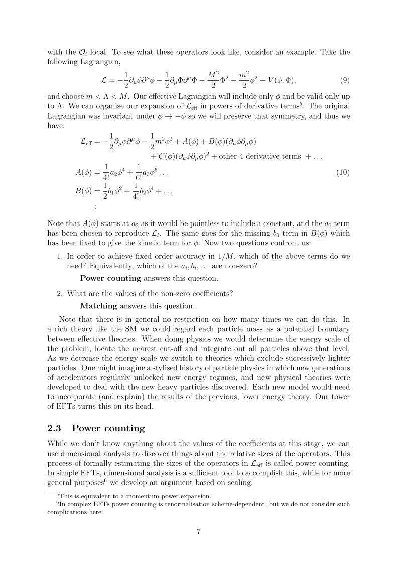
Note that A(φ) starts at a2 as it would be pointless to include a constant, and the a1 termhas been chosen to reproduce Ll. The same goes for the missing b0 term in B(φ) whichhas been fixed to give the kinetic term for φ. Now two questions confront us:

1. In order to achieve fixed order accuracy in 1/M , which of the above terms do weneed? Equivalently, which of the ai, bi, . . . are non-zero?

Power counting answers this question.

2. What are the values of the non-zero coefficients?

Matching answers this question.

Note that there is in general no restriction on how many times we can do this. Ina rich theory like the SM we could regard each particle mass as a potential boundarybetween effective theories. When doing physics we would determine the energy scale ofthe problem, locate the nearest cut-off and integrate out all particles above that level.As we decrease the energy scale we switch to theories which exclude successively lighterparticles. One might imagine a stylised history of particle physics in which new generationsof accelerators regularly unlocked new energy regimes, and new physical theories weredeveloped to deal with the new heavy particles discovered. Each new model would needto incorporate (and explain) the results of the previous, lower energy theory. Our towerof EFTs turns this on its head.

2.3 Power counting

While we don’t know anything about the values of the coefficients at this stage, we canuse dimensional analysis to discover things about the relative sizes of the operators. Thisprocess of formally estimating the sizes of the operators in Leff is called power counting.In simple EFTs, dimensional analysis is a sufficient tool to accomplish this, while for moregeneral purposes6 we develop an argument based on scaling.

5This is equivalent to a momentum power expansion.6In complex EFTs power counting is renormalisation scheme-dependent, but we do not consider such

complications here.

7

2.3.1 Naıve dimensional analysis

I’ll demonstrate the dimensional analysis argument in D dimensions7 and then workthrough a scaling example for D = 4. We work in natural units (~ = c = 1) so that[mass]=[energy]=[length]−1. All dimensions are expressed in units of [mass] so that wesimply refer to the exponent as the “dimension”. Now

∫dDxL must be dimensionless

and [dDx] = −D, so L has mass dimension D. Each term in L must therefore alsohave dimension D. We calculate the dimensions of the fields from the kinetic term inthe Lagrangian8. So for a scalar field we have ∂µφ∂

µφ, and as [∂µ] = 1, [φ] = D/2 − 1.Fermionic kinetic terms look like iψ 6∂ψ, so we have [ψ] = (D − 1)/2.

Once we have the dimension of the fields, we can easily arrive at the dimensions ofthe operators. By the same logic as above, if the dimension of operator Oi is δi then itscoupling gi has dimension D − δi. For convenience we define dimensionless couplings

λi ≡gi

ΛD−δi(11)

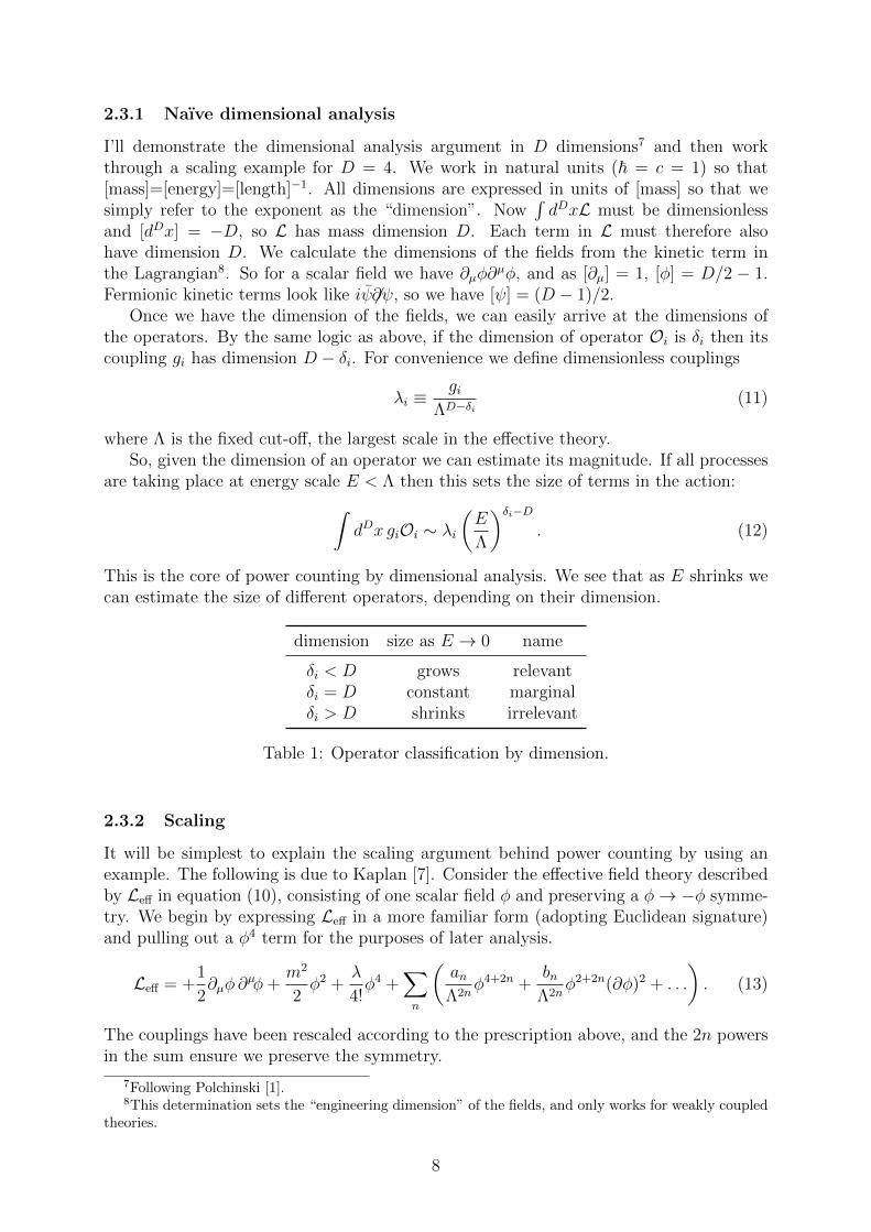
where Λ is the fixed cut-off, the largest scale in the effective theory.So, given the dimension of an operator we can estimate its magnitude. If all processes

are taking place at energy scale E < Λ then this sets the size of terms in the action:∫dDx giOi ∼ λi

(E

Λ

)δi−D. (12)

This is the core of power counting by dimensional analysis. We see that as E shrinks wecan estimate the size of different operators, depending on their dimension.

dimension size as E → 0 name

δi < D grows relevantδi = D constant marginalδi > D shrinks irrelevant

Table 1: Operator classification by dimension.

2.3.2 Scaling

It will be simplest to explain the scaling argument behind power counting by using anexample. The following is due to Kaplan [7]. Consider the effective field theory describedby Leff in equation (10), consisting of one scalar field φ and preserving a φ→ −φ symme-try. We begin by expressing Leff in a more familiar form (adopting Euclidean signature)and pulling out a φ4 term for the purposes of later analysis.

Leff = +1

2∂µφ ∂

µφ+m2

2φ2 +

λ

4!φ4 +

∑n

(anΛ2n

φ4+2n +bn

Λ2nφ2+2n(∂φ)2 + . . .

). (13)

The couplings have been rescaled according to the prescription above, and the 2n powersin the sum ensure we preserve the symmetry.

7Following Polchinski [1].8This determination sets the “engineering dimension” of the fields, and only works for weakly coupled

theories.

8

Suppose we scale the field, by taking φ(x)→ φs(x) = φ(sx). This would yield

SW [φs(x)] =

∫d4x

1

2(∂xφ(sx))2 +

m2

2φ(sx)2 +

λ

4!φ(sx)4

+∑n

(anΛ2n

φ4+2n(sx) +bn

Λ2n(∂xφ(sx))2φ2+2n(sx) + . . .

).

Now define a new variable y = sx. Then d4x = s−4d4y, ∂x = s∂y. Also define φ(y) =s−1φ(y). Then we have

SW [φ(y)] =

∫d4y

1

2(∂yφ(y))2 +

m2s−2

2φ(y)2 +

λ

4!φ(y)4

+∑n

(ans

2n

Λ2nφ4+2n(y) +

bns2n

Λ2n(∂yφ(y))2φ2+2n(y) + . . .

). (14)

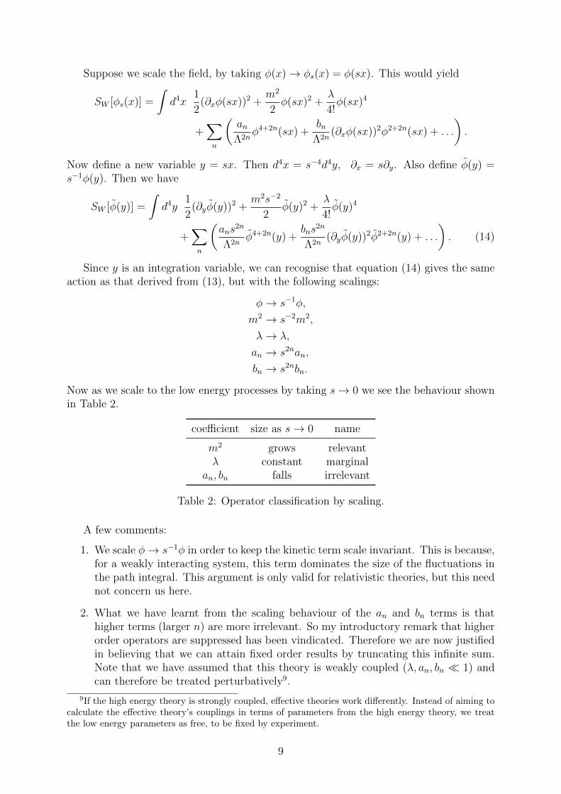
Since y is an integration variable, we can recognise that equation (14) gives the sameaction as that derived from (13), but with the following scalings:

φ→ s−1φ,

m2 → s−2m2,

λ→ λ,

an → s2nan,

bn → s2nbn.

Now as we scale to the low energy processes by taking s→ 0 we see the behaviour shownin Table 2.

coefficient size as s→ 0 name

m2 grows relevantλ constant marginal

an, bn falls irrelevant

Table 2: Operator classification by scaling.

A few comments:

1. We scale φ→ s−1φ in order to keep the kinetic term scale invariant. This is because,for a weakly interacting system, this term dominates the size of the fluctuations inthe path integral. This argument is only valid for relativistic theories, but this neednot concern us here.

2. What we have learnt from the scaling behaviour of the an and bn terms is thathigher terms (larger n) are more irrelevant. So my introductory remark that higherorder operators are suppressed has been vindicated. Therefore we are now justifiedin believing that we can attain fixed order results by truncating this infinite sum.Note that we have assumed that this theory is weakly coupled (λ, an, bn � 1) andcan therefore be treated perturbatively9.

9If the high energy theory is strongly coupled, effective theories work differently. Instead of aiming tocalculate the effective theory’s couplings in terms of parameters from the high energy theory, we treatthe low energy parameters as free, to be fixed by experiment.

9

3. Note, however, that the term “irrelevant” is somewhat misleading. These termsshould not simply be ignored and indeed often contain important information aboutthe underlying high energy dynamics.

2.3.3 Naturalness

There is one further constraint on effective theories, beyond symmetries and locality ofoperators, which had to wait on an explanation of power counting. This is the constraintof “naturalness”, which is variously described as anything from an aesthetic constraintto a major problem for a theory. For a theory to be natural, its dimensionless couplings(λi) should be of order 1, while the dimensionful couplings (gi) should be of the order ofthe heavy scale (M). Looking at how I defined the λi above, it is clear that both canbe satisfied. However, there is a problem arising from this, which concerns mass terms.Consider the φ2 term, which has dimension 2 for D = 4. The dimensionless coupling λ forthis term will be of order 1, which means the dimension-cancelling Λ2 will set the scale.But now the Lagrangian contains

1

2m2φ2 =

1

2(2λΛ2)φ2,

a mass term for φ with the mass of the order of Λ — the cut-off! If this is so, this fieldshould not be in our effective theory at all.

Therefore, in order for a theory to be natural it cannot contain mass terms. Moreprecisely, natural theories are those where all mass terms are forbidden by symmetries.Note that this does not mean our effective theories cannot deal with physically massiveobjects. It simply means that masses can only arise from spontaneously broken high-energy symmetries.

The Standard Model is not natural. While we could explain the masses of the W andZ bosons as being due to the broken electroweak symmetry (the fields they originate fromare massless prior to SSB), there is no symmetry forbidding a mass term for the Higgs.

2.4 Tree-level matching

Matching too is easiest explained using an example. This provides the first opportunityto apply some of the ideas developed so far. The aim of a matching calculation is to fixthe values of the effective coefficients in Leff so that we reproduce the predictions of thefull theory to fixed accuracy. This is one of the two ways in which the high-energy theorydetermines the content of the effective theory, with the other being the application ofsymmetry constraints.

Following Burgess [2] I will use the classic complex scalar field Lagrangian with SSB,as it provides us with naturally separated fields — a light (massless) Goldstone boson anda heavy field.

L = −∂µφ∗∂µφ−λ2

4

(φ∗φ− v2

)2

(15)

Written in the form of equation (15) it is clear that we have a symmetry φ → εiωφ, for∂µω = 0. In order to highlight this we adopt the field redefinition

φ ≡ χeiθ (16)

10

so that (15) becomes

L = −∂µχ∂µχ− χ2∂µθ∂µθ − λ2

4

(χ2 − v2

)2

. (17)

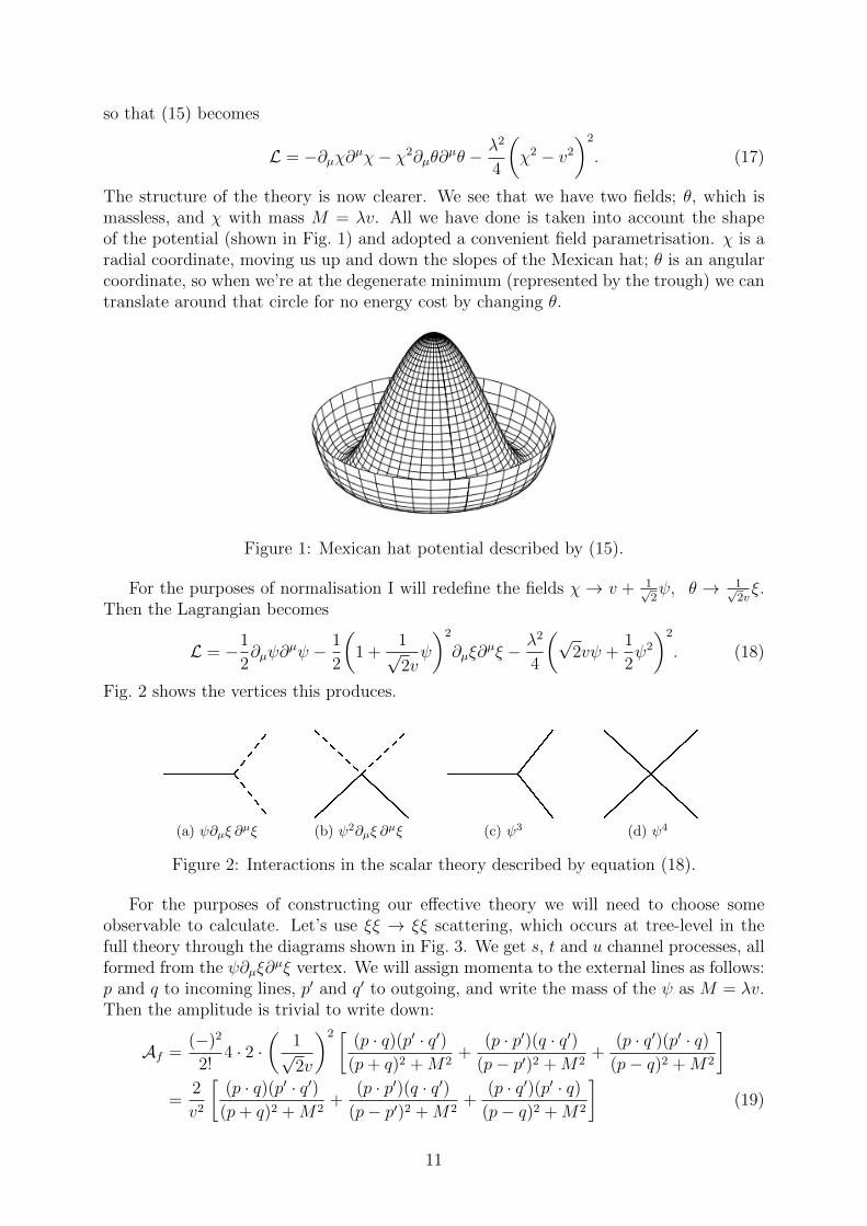
The structure of the theory is now clearer. We see that we have two fields; θ, which ismassless, and χ with mass M = λv. All we have done is taken into account the shapeof the potential (shown in Fig. 1) and adopted a convenient field parametrisation. χ is aradial coordinate, moving us up and down the slopes of the Mexican hat; θ is an angularcoordinate, so when we’re at the degenerate minimum (represented by the trough) we cantranslate around that circle for no energy cost by changing θ.

Figure 1: Mexican hat potential described by (15).

For the purposes of normalisation I will redefine the fields χ → v + 1√2ψ, θ → 1√

2vξ.

Then the Lagrangian becomes

L = −1

2∂µψ∂

µψ − 1

2

(1 +

1√2vψ

)2

∂µξ∂µξ − λ2

4

(√2vψ +

1

2ψ2

)2

. (18)

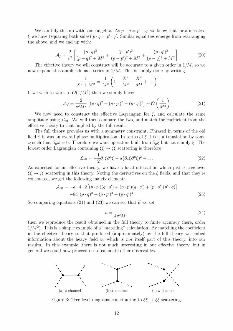
Fig. 2 shows the vertices this produces.

�(a) ψ∂µξ ∂

µξ�

(b) ψ2∂µξ ∂µξ�

(c) ψ3

�(d) ψ4

Figure 2: Interactions in the scalar theory described by equation (18).

For the purposes of constructing our effective theory we will need to choose someobservable to calculate. Let’s use ξξ → ξξ scattering, which occurs at tree-level in thefull theory through the diagrams shown in Fig. 3. We get s, t and u channel processes, allformed from the ψ∂µξ∂

µξ vertex. We will assign momenta to the external lines as follows:p and q to incoming lines, p′ and q′ to outgoing, and write the mass of the ψ as M = λv.Then the amplitude is trivial to write down:

Af =(−)2

2!4 · 2 ·

(1√2v

)2 [(p · q)(p′ · q′)

(p+ q)2 +M2+

(p · p′)(q · q′)(p− p′)2 +M2

+(p · q′)(p′ · q)

(p− q)2 +M2

]=

2

v2

[(p · q)(p′ · q′)

(p+ q)2 +M2+

(p · p′)(q · q′)(p− p′)2 +M2

+(p · q′)(p′ · q)

(p− q)2 +M2

](19)

11

We can tidy this up with some algebra. As p+ q = p′+ q′ we know that for a masslessξ we have (squaring both sides) p · q = p′ · q′. Similar equalities emerge from rearrangingthe above, and we end up with:

Af =2

v2

[(p · q)2

(p+ q)2 +M2+

(p · p′)2

(p− p′)2 +M2+

(p · q′)2

(p− q)2 +M2

](20)

The effective theory we will construct will be accurate to a given order in 1/M , so wenow expand this amplitude as a series in 1/M . This is simply done by writing

1

X2 +M2=

1

M2

(1− X2

M2+X4

M4+ . . .

)If we wish to work to O(1/M2) then we simply have:

Af =2

v2M2

[(p · q)2 + (p · p′)2 + (p · q′)2

]+O

(1

M2

)(21)

We now need to construct the effective Lagrangian for ξ, and calculate the sameamplitude using Leff. We will then compare the two, and match the coefficient from theeffective theory to that implied by the full result.

The full theory provides us with a symmetry constraint. Phrased in terms of the oldfield φ it was an overall phase multiplication. In terms of ξ this is a translation by someω such that ∂µω = 0. Therefore we want operators built from ∂µξ but not simply ξ. Thelowest order Lagrangian containing ξξ → ξξ scattering is therefore

Leff = −1

2∂µξ∂

µξ − a(∂µξ∂

µξ)2 + . . . (22)

As expected for an effective theory, we have a local interaction which just is tree-levelξξ → ξξ scattering in this theory. Noting the derivatives on the ξ fields, and that they’recontracted, we get the following matrix element:

Aeff = −a · 4 · 2[(p · p′)(q · q′) + (p · p′)(q · q′) + (p · q′)(p′ · q)

]= −8a

[(p · q)2 + (p · p′)2 + (p · q′)2

](23)

So comparing equations (21) and (23) we can see that if we set

a =1

4v2M2(24)

then we reproduce the result obtained in the full theory to finite accuracy (here, order1/M2). This is a simple example of a “matching” calculation. By matching the coefficientin the effective theory to that produced (approximately) by the full theory we embedinformation about the heavy field ψ, which is not itself part of this theory, into ourresults. In this example, there is not much interesting in our effective theory, but ingeneral we could now proceed on to calculate other observables.

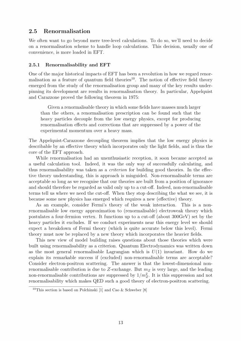
�(a) s channel�

(b) t channel�

(c) u channel

Figure 3: Tree-level diagrams contributing to ξξ → ξξ scattering.

12

2.5 Renormalisation

We often want to go beyond mere tree-level calculations. To do so, we’ll need to decideon a renormalisation scheme to handle loop calculations. This decision, usually one ofconvenience, is more loaded in EFT.

2.5.1 Renormalisability and EFT

One of the major historical impacts of EFT has been a revolution in how we regard renor-malisation as a feature of quantum field theories10. The notion of effective field theoryemerged from the study of the renormalisation group and many of the key results under-pinning its development are results in renormalisation theory. In particular, Appelquistand Carazzone proved the following theorem in 1975:

Given a renormalisable theory in which some fields have masses much largerthan the others, a renormalisation prescription can be found such that theheavy particles decouple from the low energy physics, except for producingrenormalisation effects and corrections that are suppressed by a power of theexperimental momentum over a heavy mass.

The Appelquist-Carazzone decoupling theorem implies that the low energy physics isdescribable by an effective theory which incorporates only the light fields, and is thus thecore of the EFT approach.

While renormalisation had an unenthusiastic reception, it soon became accepted asa useful calculation tool. Indeed, it was the only way of successfully calculating, andthus renormalisability was taken as a criterion for building good theories. In the effec-tive theory understanding, this is approach is misguided. Non-renormalisable terms areacceptable so long as we recognise that our theories are built from a position of ignoranceand should therefore be regarded as valid only up to a cut-off. Indeed, non-renormalisableterms tell us where we need the cut-off. When they stop describing the what we see, it isbecause some new physics has emerged which requires a new (effective) theory.

As an example, consider Fermi’s theory of the weak interaction. This is a non-renormalisable low energy approximation to (renormalisable) electroweak theory whichpostulates a four-fermion vertex. It functions up to a cut-off (about 300GeV) set by theheavy particles it excludes. If we conduct experiments near this energy level we shouldexpect a breakdown of Fermi theory (which is quite accurate below this level). Fermitheory must now be replaced by a new theory which incorporates the heavier fields.

This new view of model building raises questions about those theories which werebuilt using renormalisability as a criterion. Quantum Electrodynamics was written downas the most general renormalisable Lagrangian which is U(1) invariant. How do weexplain its remarkable success if (excluded) non-renormalisable terms are acceptable?Consider electron-positron scattering. The answer is that the lowest-dimensional non-renormalisable contribution is due to Z-exchange. But mZ is very large, and the leadingnon-renormalisable contributions are suppressed by 1/m2

Z . It is this suppression and notrenormalisability which makes QED such a good theory of electron-positron scattering.

10This section is based on Polchinski [1] and Cao & Schweber [8]

13

2.5.2 Renormalisation schemes and EFTs

A renormalisation scheme consists of a method for making infinite integrals finite (aregulator) and a method for dealing with the infinite part (a subtraction scheme). Thesecan broadly be classified in terms of the mass-dependence of the subtraction scheme.Physical quantities cannot depend on our choice of renormalisation scheme, so this isusually a choice of convenience of preference. In the context of effective field theory,however, Bain [6] and Georgi [9, 10] argue that the choice implies a conception of howEFTs function. The choice is broadly between mass-dependent schemes (which go with a‘Wilsonian’ formulation of EFT) and mass-independent schemes (which go with Georgi’s‘continuum EFT’ formulation).

The presence of the effective theory cut-off Λ makes a momentum cut-off regularisationseem appropriate. This directly implements the idea that in EFT we calculate only belowΛ. Furthermore, as Georgi [10] notes, the Appelquist-Carazzone theorem requires a mass-dependent scheme to operate: in a mass-independent scheme “the renormalisation scaledependence [in, e.g., SU(5)] of the Feynman graphs are the same whether there is a gluonor an X particle inside.” So the decoupling which in some sense justifies the EFT is onlyformally guaranteed under such a scheme.

However, there are a number of disadvantages to mass-dependent renormalisation.Firstly, such schemes violate Poincare and gauge invariance. To see this, note that wecan Fourier transform our regulated momentum-space integral, and arrive at a coordinatespace integral over a finite region. It is this volume restriction which violates Poincareinvariance, and its absence which lends Georgi’s formulation the name “continuum” EFT.

Secondly, mass-dependent schemes make loop calculations in EFTs exceedingly diffi-cult, as the mass-dependence leads to large dimensionful factors appearing in the numer-ators of higher-order terms, disrupting the suppression by inverse powers of the cut-off.The formal and principled reasons for adopting such a scheme are, to Georgi at least,outweighed by how difficult they make the business of doing physics.

Mass-independent schemes, such as dimensional regularisation and modified minimalsubtraction, correct for these latter flaws. They preserve the symmetries of the highertheory, and lead to logarithmic (but not power law) dependence on the heavy scale.Thus, we can count powers of 1/Λ as described above and are guaranteed suppression ofirrelevant terms.

How do we deal with the lack of guaranteed decoupling? The answer to this is whatmotivates Bain to describe the choice of renormalisation scheme as a conceptual dis-agreement about how EFT works. In the Wilsonian formulation decoupling underlies theformation of an EFT. For Georgi, it is “put in by hand in matching.” The two formula-tions also lead to the major calculation difference described in section 2.2; in WilsonianEFT the effective action is defined by a path integral, while in continuum EFT we simplywrite down Leff.

2.5.3 Higher-order matching

In this section I will sketch how matching works at higher orders in a loop expansion,working with in a mass-independent scheme11. At one-loop level, we will need to regulariseboth the full and effective theory using dimensional regularisation. In the full theory, werenormalise using MS. In the effective theory we renormalise by demanding that the

11This section is based on Pich [11] and Kaplan [12].

14

renormalised coupling coefficients match those in the full theory. Matching proceeds inthis way, order by order. The previous order effective coupling constant is that which ismodified by the renormalisation-matching calculation.

Let’s start by taking the theory described by equation (9) and choosing V (φ,Φ) =λ/2φ2Φ.

L = −1

2∂µφ∂

µφ− 1

2∂µΦ∂µΦ− M2

2Φ2 − m2

2φ2 − λ

2φ2Φ (25)

In the full theory φφ→ φφ scattering occurs via Φ exchange. In our effective theory, thisis replaced by the φ4 term. The effective Lagrangian is that of (13). I’ll write the firstfew terms below, using general coefficients:

Leff =a

2∂µφ ∂

µφ+b

2φ2 +

c

4!φ4 + . . . (26)

At tree-level, a = 1, b = m2 and the matching calculation for c is essentially similar tothat done in section 2.4 and results in c = 3λ/M2.

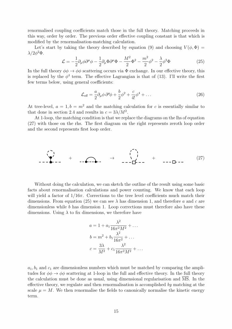
At 1-loop, the matching condition is that we replace the diagrams on the lhs of equation(27) with those on the rhs. The first diagram on the right represents zeroth loop orderand the second represents first loop order.

+ → + (27)

Without doing the calculation, we can sketch the outline of the result using some basicfacts about renormalisation calculations and power counting. We know that each loopwill yield a factor of 1/16π. Corrections to the tree level coefficients much match theirdimensions. From equation (25) we can see λ has dimension 1, and therefore a and c aredimensionless while b has dimension 1. Loop corrections must therefore also have thesedimensions. Using λ to fix dimensions, we therefore have

a = 1 + a1λ2

16π2M2+ . . .

b = m2 + b1λ2

16π2+ . . .

c =3λ

M2+ c1

λ2

16π2M2+ . . .

a1, b1 and c1 are dimensionless numbers which must be matched by comparing the ampli-tudes for φφ→ φφ scattering at 1-loop in the full and effective theory. In the full theorythe calculation must be done as usual, using dimensional regularisation and MS. In theeffective theory, we regulate and then renormalisation is accomplished by matching at thescale µ = M . We then renormalise the fields to canonically normalise the kinetic energyterm.

15

3 Bottom-Up EFTs and the PEW Measurements

3.1 Introduction

We now turn to the application of effective field theories where the UV theory is notknown12. The main application is in extending our physical theories beyond the StandardModel (SM). The basic idea is simple. We know that below the electroweak scale the SMis a good theory, showing excellent agreement with experiment. We will use it as a baseto construct an effective theory that includes the SM Lagrangian and an infinite sum oflocal operators.

Suppose LBSM represents the unknown UV theory, consisting of the SM field contentφSM and new fields ϕ13. Then if we suppose that the new fields are heavier than φSM

(which is reasonable as they represent undetected particles) we know we can write aneffective theory in the manner of equation (8):

LBSM[φSM, ϕ]→ Leff[φSM] = LSM +∑i

giOi(φSM). (28)

Note a few important features equation (28). First, it contains the Standard Model asLl; this is required as we want to reproduce our current results by extension of the SM.Second, as we’ve come to expect, the effective Lagrangian does not dependent on thenew field content ϕ of LBSM as these fields have been integrated out. This is importanthere because it means the methods we will discuss here are independent of any particularmodel of physics beyond the Standard Model (BSM). Our aim is to discuss a generalenough framework that one could simple “plug in” a favoured model.

In doing this we have to make a number of assumptions:

1. The new physics decouples, in the manner suggested by the Appelquist-Carazzonetheorem. i.e. The heavy fields decouple in the limit Λ → ∞ where Λ is a cut-offinitially set at the characteristic scale of the new physics.

2. Since the physics of electroweak symmetry breaking is not experimentally confirmedwe have to make an assumption about the Higgs sector. For the purposes of thispaper I will assume that EW symmetry is broken by a Higgs doublet. What thismeans is outlined below in section 3.2.1.

The core work in applying EFT techniques to analysing potential models of newphysics is in seeing how those models would contribute to various local operators.

In the rest of this section I will look at the use of the precision electroweak mea-surements to constrain a class of effective operators called “oblique” operators. As thisrequires some facility with the physics of the SM, I begin with some background. I thenbriefly discuss the PEW measurements, motivating their use. I then turn in section 3.3to discussing how dimension 6 oblique operators constrain additions to the SM. Finally,in section 3.4 I give a high level discussion of one model of new physics and how can beconstrained using these methods.

12This introductory section is based on the introduction in de Blas Mateo [13] and Skiba [5].13Note that there is no guarantee that the new theory will be formulated in terms of the familiar

SM physical fields, or the SU(2) × U(1) gauge fields. There could be higher symmetries which breakspontaneously to yield the SM fields. But up to such field redefinitions the above statement is a reasonableway of thinking about how a UV theory (of which the SM is a low energy effective theory) would beconstituted.

16

3.2 Background

In this section I explain various pieces of the physics of the Standard Model which arerequired for a meaningful discussion of using EFTs to constrain new physics.

3.2.1 Electroweak symmetry breaking

In order to explain tests of physics beyond the Standard Model14, it will be useful toreview some of of the physics of the electroweak sector, in particular electroweak sym-metry breaking (EWSB). This portion of the SM is all that still requires experimentalconfirmation. The theoretical addition which accomplishes EWSB in the SM is the “Higgsmechanism”, which introduces a doublet of scalar fields to the SM Lagrangian:

H =

(φ+

φ0

),

with LagrangianLHiggs = (DµH)†(DµH)− µ2H†H + λ(H†H)2.

This field has a non-zero vacuum expectation value (vev). H is expanded around the vev,which yields

H = U(

0v+h√

2

).

The U is a unitary term which turns out to be unimportant. The upshot of this is thatthe expansion about the Higgs vev brings about spontaneous symmetry breaking. Thecovariant derivative Dµ contains interactions with the electroweak gauge fields:

Dµ = ∂µ +i

2g1Bµ +

i

2g2τ

aW aµ (29)

The result is that the Higgs Lagrangian can be expanded out as

LHiggs =1

2∂µh∂

µh+1

8(g2

1 + g22)(Bµ −W3µ)(Bµ −W µ

3 )(v + h)2

+g2

2

8(W1µ − iW2µ)(W µ

1 − iWµ2 )(v + h)2

+ terms involving just h

From the second and third terms we can identify physical fields made from combinationsof the gauge fields Bµ and Waµ. This is done by expanding the (v + h)2 and looking forterms with the form of mass terms. This leads to a set of field redefinitions which takeus from the gauge fields to the physical fields of the photon, W± and Z boson. For thephoton and Z boson we can represent the transformation from the gauge fields to thephysical fields as a rotation through an angle θW called the Weinberg weak mixing angle:(

Zµ

Aµ

)=

(cos θW − sin θWsin θW cos θW

)(W µ

3

Bµ

)(30)

This angle is defined by

sin2 θW =g2

1

g21 + g2

2

(31)

14This section is based on my notes from Dr Matthew Wingate’s course on the Standard Model as wellas Dr Hugh Osborn’s set of notes [14].

17

Writing sW = sin θW and cW = cos θW , the field redefinitions are

Aµ ≡ cWW3µ + sWBµ,

Zµ ≡ cWW3µ − sWBµ,

W−µ ≡

1√2

(W1µ + iW2µ),

W+µ ≡

1√2

(W1µ − iW2µ).

This leads to the following relation between the masses of the Z and W bosons

mW

mZ

= cos θW , (32)

which can be written in terms of the Higgs vev and gauge couplings as

m2Z =

v2

4(g2

1 + g22), (33)

m2W =

g22v

2

4. (34)

3.2.2 Custodial symmetry

We can convert the above relation between W and Z into a single parameter ρ defined as

ρ =m2W

m2Z cos2 θW

. (35)

At tree-level in the SM we know that ρ = 1. It is possible that there are higher orderradiative corrections to this, which would arise from processes which shift the Z masswithout changing the W mass (or vice versa). It is possible to theoretically disallow suchterms by positing a larger global symmetry group than is currently part of the SM.

The EW sector has the symmetry breaking structure

SU(2)L × U(1)Y → U(1)QED.

Under this new proposal, we introduce a symmetry which groups right-handed fermionsinto SU(2) doublets. This SU(2)R symmetry is global. We gauge only the U(1) portionof it and are left, after symmetry breaking, with SU(2)cust × U(1)QED. This additionalsymmetry explicitly forbids terms which change ρ from unity.

This has led to a habit of referring to any new physics which results in ρ 6= 1 as“breaking custodial symmetry”. Below, this should be taken to mean only that theseprocesses shift the mass of either the Z or W bosons, and nothing more.

3.2.3 Vacuum polarisation

The particular type of new physics discussed below affects the self-energies of the W and Zbosons15. In QFT, propagators receive loop corrections due to the production of fermion–anti-fermion loops, as shown in Fig. 4. This leads to a phenomenon known as vacuumpolarisation. As the fermion and anti-fermion carry opposite charge, they form a dipole as

15Formulae in this section are taken from Ryder [15].

18

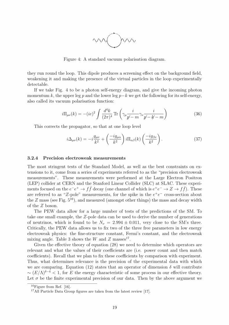
Figure 4: A standard vacuum polarisation diagram.

they run round the loop. This dipole produces a screening effect on the background field,weakening it and making the presence of the virtual particles in the loop experimentallydetectable.

If we take Fig. 4 to be a photon self-energy diagram, and give the incoming photonmomentum k, the upper leg p and the lower leg p−k we get the following for its self-energy,also called its vacuum polarisation function:

iΠµν(k) = −(ie)2

∫d4k

(2π)4Tr

(γµ

i

6p−mγν

i

6p− 6k −m

)(36)

This corrects the propagator, so that at one loop level

i∆µν(k) = −igµνk2

+

(−igµαk2

)iΠαβ(k)

(−igβνk2

). (37)

3.2.4 Precision electroweak measurements

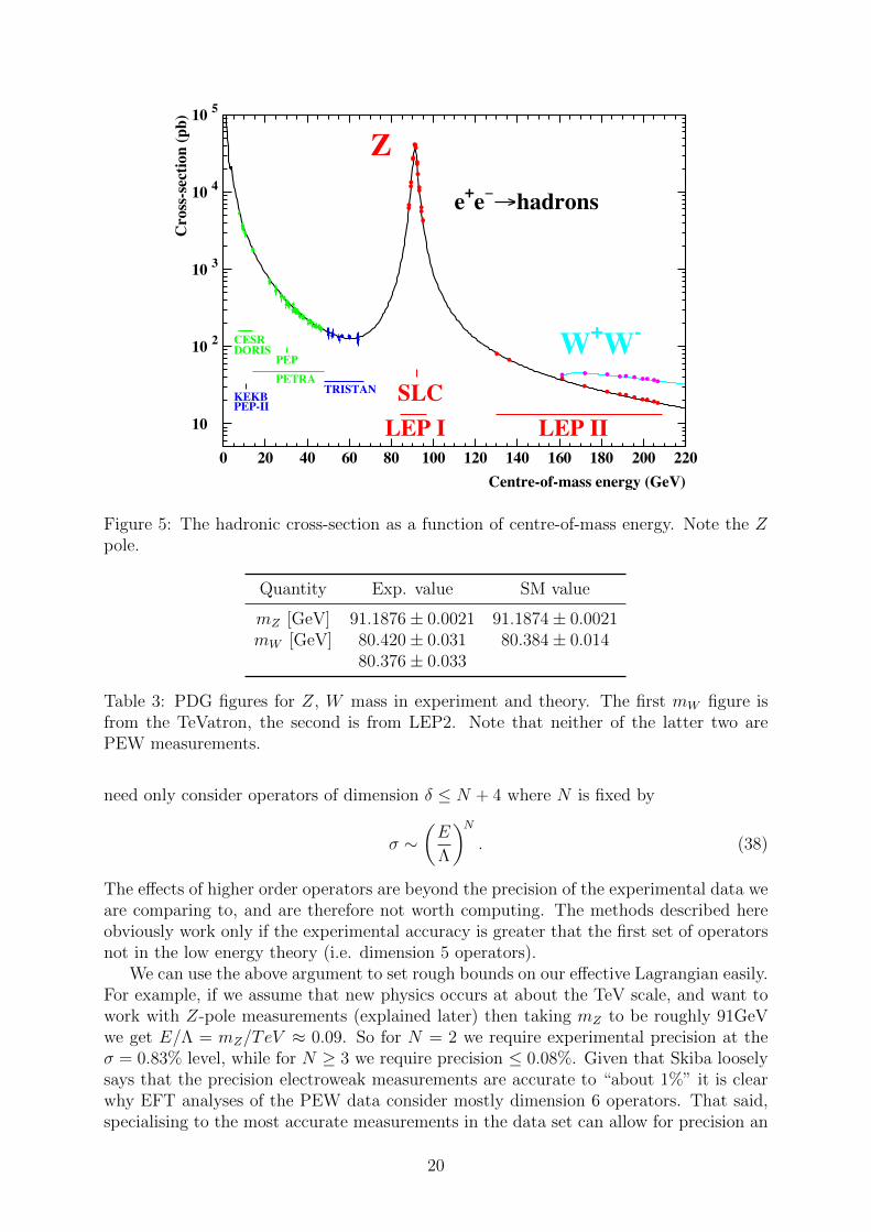
The most stringent tests of the Standard Model, as well as the best constraints on ex-tensions to it, come from a series of experiments referred to as the “precision electroweakmeasurements”. These measurements were performed at the Large Electron Positron(LEP) collider at CERN and the Stanford Linear Collider (SLC) at SLAC. These experi-ments focused on the e−e+ → ff decay (one channel of which is e+e− → Z → ff). Theseare referred to as “Z-pole” measurements, for the spike in the e+e− cross-section aboutthe Z mass (see Fig. 516), and measured (amongst other things) the mass and decay widthof the Z boson.

The PEW data allow for a large number of tests of the predictions of the SM. Totake one small example, the Z-pole data can be used to derive the number of generationsof neutrinos, which is found to be Nν = 2.994 ± 0.011, very close to the SM’s three.Critically, the PEW data allows us to fix two of the three free parameters in low energyelectroweak physics: the fine-structure constant, Fermi’s constant, and the electroweakmixing angle. Table 3 shows the W and Z masses17.

Given the effective theory of equation (28) we need to determine which operators arerelevant and what the values of their coefficients are (i.e. power count and then matchcoefficients). Recall that we plan to fix these coefficients by comparison with experiment.Thus, what determines relevance is the precision of the experimental data with whichwe are comparing. Equation (12) states that an operator of dimension δ will contribute∼ (E/Λ)δ−4 < 1, for E the energy characteristic of some process in our effective theory.Let σ be the finite experimental precision of our data. Then by the above argument we

16Figure from Ref. [16].17All Particle Data Group figures are taken from the latest review [17].

19

10

10 2

10 3

10 4

10 5

0 20 40 60 80 100 120 140 160 180 200 220Centre-of-mass energy (GeV)

Cro

ss-s

ectio

n (p

b)

CESRDORIS

PEPPETRA

TRISTANKEKBPEP-II

SLCLEP I LEP II

Z

W+W-

e+e<Ahadrons

Figure 5: The hadronic cross-section as a function of centre-of-mass energy. Note the Zpole.

Quantity Exp. value SM value

mZ [GeV] 91.1876± 0.0021 91.1874± 0.0021mW [GeV] 80.420± 0.031 80.384± 0.014

80.376± 0.033

Table 3: PDG figures for Z, W mass in experiment and theory. The first mW figure isfrom the TeVatron, the second is from LEP2. Note that neither of the latter two arePEW measurements.

need only consider operators of dimension δ ≤ N + 4 where N is fixed by

σ ∼(E

Λ

)N. (38)

The effects of higher order operators are beyond the precision of the experimental data weare comparing to, and are therefore not worth computing. The methods described hereobviously work only if the experimental accuracy is greater that the first set of operatorsnot in the low energy theory (i.e. dimension 5 operators).

We can use the above argument to set rough bounds on our effective Lagrangian easily.For example, if we assume that new physics occurs at about the TeV scale, and want towork with Z-pole measurements (explained later) then taking mZ to be roughly 91GeVwe get E/Λ = mZ/TeV ≈ 0.09. So for N = 2 we require experimental precision at theσ = 0.83% level, while for N ≥ 3 we require precision ≤ 0.08%. Given that Skiba looselysays that the precision electroweak measurements are accurate to “about 1%” it is clearwhy EFT analyses of the PEW data consider mostly dimension 6 operators. That said,specialising to the most accurate measurements in the data set can allow for precision an

20

order of magnitude greater, allowing us to stretch our analysis to higher-order operators.By contrast, LEP2 measurements of the W mass are an order of magnitude less precise.

3.3 Effective operators

3.3.1 The Peskin-Takeuchi parameters

In a 1991 paper Peskin and Takeuchi derived a set of three parameters, labelled S, T andU which capture the effect of new physics to the electroweak sector. Roughly speaking Sparameterises the ‘size’ of the new sector and T captures the total weak-isospin breakingit introduces. S and T parameterise the effects of dimension six operators, which will beconsidered here, while U parameterises effects due to dimension eight operators, and willtherefore not be discussed.

We can make the above meaning of T more specific. T breaks custodial symmetrydirectly:

ρ = 1 + δρSM + αT,

where δρSM term is to account for any high loop corrections which may be calculated.The PDG currently lists the following as the measured value of ρ:

ρPEW = 1.0008+0.0017−0.0007.

In deriving S, T and U a few assumptions are made about the new physics sector:

1. The electroweak gauge group is unaffected by the new physics (so, in particular, itdoes not include new EW bosons).

2. The new fields do not couple to SM fermions. This condition defines an “oblique”operator.

3. The energy scale at which the new physics appears is large compared to the elec-troweak scale.

A clear definition of these parameters (taken from Hewett [18]) in terms of vacuum po-larisation functions of the electroweak bosons is

αS = 4s2W c

2W

(Π′ZZ(0)− c2

W − s2W

sW cWΠ′Zγ(0)− Π′γγ(0)

), (39)

αT =( 1

m2W

ΠWW (0)− 1

m2Z

ΠZZ(0)), (40)

αU = 4s2W

(Π′WW (0)− c2

WΠ′ZZ(0)− 2sW cWΠ′Zγ(0)− s2WΠγγ(0)

). (41)

The job of testing new physics then boils down to calculating these vacuum polarisationsin the new theory, taking the derivative

Π′(XY )(0) =d

d(q2)

[Π(XY )(q

2)

]q2=0

,

and evaluating the result against the SM values. As of the last PDG review the measuredvalues are

S = 0.01± 0.10(−0.08), (42)

T = 0.03± 0.11(+0.09), (43)

U = 0.06± 0.10(+0.01). (44)

These values were calculated assuming MHiggs = 117 GeV and the corrections in paren-theses show the difference if we instead assume MHiggs = 300 GeV.

21

3.3.2 Oblique operators

There are obviously a large number of dimension 6 operators we can form from the fieldsof the SM18. For any observable in our new theory, we expect that predictions for thatoperator will take the form

Xpred = XSM +∑i

aiXi,

where XSM is the prediction for that observable in the SM and the Xi are the correctionsintroduced for each Oi. Not all operators contribute to all observables, of course. Thosethat do contribute might do so in one of two ways, which we call direct and indirect.A direct correction comes from the introduction of a new channel for the process thatobservable derives from. So, if we are considering the process e+e− → µ+µ− and theobservable is the cross-section, then we would get a direct contribution from a four-fermion operator like Oel = (¯γµ`)(eγµe). An indirection contribution, on the other hand,arises from a correction to processes used in measuring input parameters such as α,GF

and mZ . Since these are used as inputs to calculate other observables, those all receivecorrections from these shifts.

We will focus on the class of operators which do not contain fermion fields. In oureffective theory formulation these arise when the new heavy fields couple directly tothe SM gauge fields and Higgs. Since they directly correct gauge boson masses andfermion couplings, they are also referred to as ‘universal’ operators. The main reason forfocusing on such operators is that even small couplings of new physics to the SM quarksand leptons can lead to very large (experimentally disallowed) flavour changing neutralcurrents. Note that new fields which couple to the SM gauge bosons can give rise toeffective interactions involving the quarks and leptons. Luckily, the coefficients of theseoperators are suppressed both by inverse powers of Λ and by what Grinstein calls a “weakcoupling suppression factor” ∼ α/4π. Therefore they can be ignored when focusing onoblique operators.

Skiba identifies two operators as being particularly interesting:

OS = H†σiHW iµνB

µν (45)

OT =∣∣H†DµH

∣∣2 (46)

They generate the vertices shown in Fig. 6. OT introduces kinetic mixing between W 3µ

and Bµ, while OT violates custodial symmetry. These operators are interesting becausetheir couplings can be directly related to the Peskin-Takeuchi parameters:

S =4sW cWv

2

αaS, (47)

T = − v2

2αaT . (48)

3.4 Constraints on new physics

Consider a new heavy quark familyPeskin & Takeuchi introduce this example in theiroriginal paper, and Skiba discusses it in his review. (T,B) with the same structure asSM quark families (the left-handed portions form a doublet under SU(2)), hypercharge

18This section is largely based on Han [19] and Skiba [5], with minor input from Grinstein [20].

22

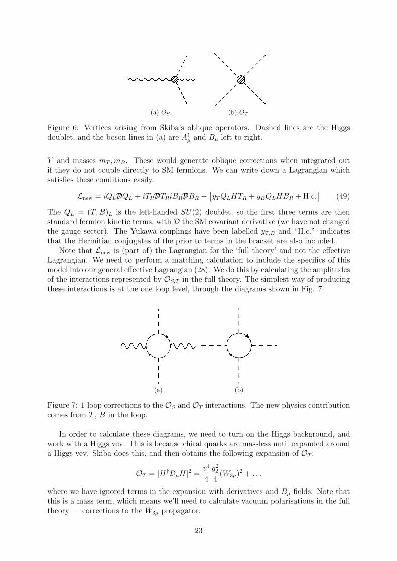
�(a) OS

�(b) OT

Figure 6: Vertices arising from Skiba’s oblique operators. Dashed lines are the Higgsdoublet, and the boson lines in (a) are Aiµ and Bµ left to right.

Y and masses mT ,mB. These would generate oblique corrections when integrated outif they do not couple directly to SM fermions. We can write down a Lagrangian whichsatisfies these conditions easily.

Lnew = iQL 6DQL + iTR 6DTRiBR 6DBR −[yT QLHTR + yBQLHBR + H.c.

](49)

The QL = (T,B)L is the left-handed SU(2) doublet, so the first three terms are thenstandard fermion kinetic terms, with D the SM covariant derivative (we have not changedthe gauge sector). The Yukawa couplings have been labelled yT,B and “H.c.” indicatesthat the Hermitian conjugates of the prior to terms in the bracket are also included.

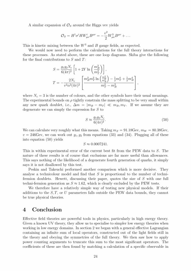
Note that Lnew is (part of) the Lagrangian for the ‘full theory’ and not the effectiveLagrangian. We need to perform a matching calculation to include the specifics of thismodel into our general effective Lagrangian (28). We do this by calculating the amplitudesof the interactions represented by OS,T in the full theory. The simplest way of producingthese interactions is at the one loop level, through the diagrams shown in Fig. 7.

(a) (b)

Figure 7: 1-loop corrections to the OS and OT interactions. The new physics contributioncomes from T , B in the loop.

In order to calculate these diagrams, we need to turn on the Higgs background, andwork with a Higgs vev. This is because chiral quarks are massless until expanded arounda Higgs vev. Skiba does this, and then obtains the following expansion of OT :

OT = |H†DµH|2 =v4

4

g22

4(W3µ)2 + . . .

where we have ignored terms in the expansion with derivatives and Bµ fields. Note thatthis is a mass term, which means we’ll need to calculate vacuum polarisations in the fulltheory — corrections to the W3µ propagator.

23

A similar expansion of OS around the Higgs vev yields

OS = H†σiHW iµνB

µν = −v2

2W 3µνB

µν + . . .

This is kinetic mixing between the W 3 and B gauge fields, as expected.We would now need to perform the calculations for the full theory interactions for

these processes. As stated above, these are one loop diagrams. Skiba give the followingfor the final contributions to S and T :

S =g1g2Nc

6(4π)2

[1 + 2Y ln

(m2B

m2T

)],

T = − 2Nc

v2α2(4π)2

m2Bm

2T ln

(m2

T

m2B

)− 1

2m4T + 1

2m4B

m2T −m2

B

,where Nc = 3 is the number of colours, and the other symbols have their usual meanings.The experimental bounds on ρ tightly constrain the mass splitting to be very small withinany new quark doublet, i.e., ∆m = |mB − mT | � mB,mT . If we assume they aredegenerate we can simply the expression for S to

S ≈ g1g2Nc

6(4π)2. (50)

We can calculate very roughly what this means. Taking mZ = 91.18Gev, mW = 80.38Gev,v = 246Gev, we can work out g1, g2 from equations (33) and (34). Plugging all of theseinto equation (50) yields

S ≈ 0.0007241.

This is within experimental error of the current best fit from the PEW data to S. Thenature of these results is of course that exclusions are far more useful than allowances.This says nothing of the likelihood of a degenerate fourth generation of quarks, it simplysays it is not disallowed by this test.

Peskin and Takeuchi performed another comparison which is more decisive. Theyanalyse a technicolour model and find that S is proportional to the number of techni-fermion doublets. Hewett, discussing their paper, quotes the size of S with one fulltechni-fermion generation as S ≈ 1.62, which is clearly excluded by the PEW tests.

We therefore have a relatively simple way of testing new physical models. If theiradditions to the S, T , or U parameters falls outside the PEW data bounds, they cannotbe true physical theories.

4 Conclusion

Effective field theories are powerful tools in physics, particularly in high energy theory.Given a known UV theory, they allow us to specialise to simpler low energy theories whenworking in low energy domains. In section 2 we began with a general effective Lagrangiancontaining an infinite sum of local operators, constructed out of the light fields still inthe theory and obeying the symmetries of the full theory. We then saw how to applypower counting arguments to truncate this sum to the most significant operators. Thecoefficients of these are then found by matching a calculation of a specific observable in

24

both the full and effective theories. In this way we derive a theory which can calculateobservables for all processes which involve just these light fields and which occur withinthe EFT’s energy range. This simplifies calculations, and can be pedagogically useful. Inaddition to this, important insights into the structure of quantum field theory have comefrom the study of EFTs, particularly regarding renormalisability as a criterion for ‘good’theories. We learn by studying EFTs that non-renormalisable interactions are acceptableas long as we cast our theory as an EFT, valid up to a cut-off.

Effective field theories also provide a useful and conceptually simple way of testingmodels of physics beyond the Standard Model. In section 3 we constructed a generaleffective theory containing the SM and a set of local operators. This can be matchedto any model of new physics, provided the new fields decouple in the large Λ limit.These methods are most adept at testing models of new physics which generate “oblique”corrections to the SM. We can constrain the effects of the general local operators bycomparison to the precision electroweak data. Rather than computing the effects of eachnew model on current observables, we relate these models to the pre-defined parametersS, T and U , which have already been constrained. This is done by determining how thenew physics contributes to oblique operators with known relations to S, T and U .

References

[1] J. Polchinski, “Effective Field Theory and the Fermi Surface,”arxiv:hep-th/9210046v2.

[2] C. Burgess, “Lecture 2a: Effective field theories (PIRSA09090017).” Video lecture,2009. http://pirsa.org/C09020. PSI.

[3] C. Burgess, “Lecture 3a: Effective field theories (PIRSA09100050).” Video lecture,2009. http://pirsa.org/C09020. PSI.

[4] C. Burgess, “Lecture 4b: Effective field theories (PIRSA09100154).” Video lecture,2009. http://pirsa.org/C09020. PSI.

[5] W. Skiba, “TASI lectures on Effective Field Theory and Precision ElectroweakMeasurements,” arxiv:hep-ph/1006.2142v1.

[6] J. Bain, “Effective Field Theories,”http://ls.poly.edu/ jbain/papers/EFTs.pdf.

[7] D. Kaplan, “Five lectures on Effective Field Theory,” arxiv:nucl-th/0510023v1.

[8] T. Cao and S. Schweber, “The Conceptual Foundations and the PhilosophicalAspects of Renormalization Theory,” Synthese 97 (1993) 33–108.

[9] H. Georgi, “Effective Field Theory,” Annual Review of Nuclear and Particle Science43 (1993) 209–252.

[10] H. Georgi, “Thoughts on Effective Field Theory,” Nuclear Physics B (Proc. Suppl.)29B (1992) 1–10.

[11] A. Pich, “Effective Field Theory,” arxiv:hep-ph/9806303.

25

[12] D. Kaplan, “Effective Field Theories,” arxiv:nucl-th/9506035v1.

[13] J. de Blas Mateo, Effective Lagrangian Description of Physics Beyond the StandardModel and Electroweak Precision Tests. PhD thesis, University of Granada, 2010.http://www-ftae.ugr.es/files/PhDThesis_JdeBlas.pdf.

[14] H. Osborn, “Part III lecture notes on the Standard Model,”damtp.cam.ac.uk/user/ho/SM.ps.

[15] L. Ryder, Quantum Field Theory. CUP, 2nd ed., 1996.

[16] The ALEPH, DELPHI, L3, OPAL, SLD Collaborations, the LEP ElectroweakWorking Group, the SLD Electroweak and Heavy Flavour Groups, “PrecisionElectroweak Measurements on the Z Resonance,” arxiv:hep-ex/0509008.

[17] K. Nakamura et al., “The Review of Particle Physics,” Journal of Physics G37(2010) 075021.

[18] J. Hewett, “The Standard Model and why we believe it,”arxiv:hep-ph/9810316v1.

[19] Z. Han and W. Skiba, “Effective Theory Analysis of Precision Electroweak Data,”arxiv:hep-ph/0412166.

[20] B. Grinstein and M. Wise, “Operator analysis for precision electroweak physics,”Physics Letters B 265 (1991) 326–34.

26