Prepared for submission to JHEP CALT-68-2864

A Consistent Effective Theory of

Long-Wavelength Cosmological Perturbations

Sean M. Carroll, Stefan Leichenauer, and Jason Pollack

California Institute of Technology, Pasadena, CA 91125, U.S.A.

E-mail: seancarroll@gmail.com, sleichen@theory.caltech.edu,

jpollack@caltech.edu

Abstract: Effective field theory provides a perturbative framework to study the evo-

lution of cosmological large-scale structure. We investigate the underpinnings of this

approach, and suggest new ways to compute correlation functions of cosmological ob-

servables. We find that, in contrast with quantum field theory, the appropriate effective

theory of classical cosmological perturbations involves interactions that are nonlocal in

time. We describe an alternative to the usual approach of smoothing the perturba-

tions, based on a path-integral formulation of the renormalization group equations.

This technique allows for improved handling of short-distance modes that are pertur-

batively generated by long-distance interactions.

arX

iv:1

310.

2920

v2 [

hep-

th]

6 N

ov 2

013

Contents

1 Introduction 1

2 Notation 4

3 The Smoothing Approach 5

3.1 Standard Perturbation Theory 5

3.2 Effective Equations of Motion 9

3.3 Effective Perturbation Theory 11

3.4 Correlation Functions 14

4 A Path Integral Approach 15

4.1 Polchinski RG 15

4.2 A Path Integral for Standard Perturbation Theory 17

4.3 RG in the Effective Theory 18

4.4 Renormalization of the One-Point Function and Power Spectrum 23

5 Conclusions and Further Directions 25

A Explicit Calculations 26

A.1 Standard Perturbation Theory 26

A.2 Accounting for the Cutoff 28

1 Introduction

Effective Field Theory (EFT) has been successful in a wide variety of contexts. It allows

a faithful description of physics at the length scales one is interested in measuring,

without requiring detailed knowledge of dynamics at shorter distances. Instead the

theory is formulated with an explicit length scale, the cutoff scale Λ−1, below which

modes can be nonlinear. The effects of short-wavelength physics appear only through

parameters of the long-wavelength equations. The precise value of the cutoff scale

is arbitrary and is chosen out of convenience, so physical quantities like correlation

functions should not depend on it. Since Λ enters calculations at intermediate stages,

the requirement that the physics be Λ-independent non-trivially constrains the resulting

long-wavelength theory.

– 1 –

Recently [1–7], the principles of EFT have been applied to the problem of Large

Scale Structure (LSS), the distribution of matter in the observable universe. Tra-

ditionally, standard perturbation theory ([8–13], reviewed in [14]) has been used to

compute the LSS correlation functions, but as has been emphasized in [1, 2], this is

not a reliable basis for the theory. The problem is that for comoving wavenumbers

k > kNL ∼ (10 Mpc)−1 the perturbations have grown large enough that they become

nonlinear. Standard perturbation theory (SPT), however, is only strictly valid when

all modes remain linear, even those with k > kNL where we know perturbation the-

ory no longer applies. Starting at second order, SPT includes backreaction due to the

propagation of modes of all wave numbers. So even for long-wavelength modes that

have remained linear to a very good approximation, we should not trust the results of

SPT at or beyond this order.

The alternative is to use EFT. The natural cutoff scale, Λ ∼ kNL, is precisely the

point where SPT breaks down. EFT treats modes with k < kNL perturbatively, but

does not attempt to make predictions about modes with k > kNL. Instead, within

the EFT there are several additional parameters (beyond those found in SPT) whose

values encode the effects that the nonlinear modes have on the linear modes. These

parameters are not calculable within the EFT itself; they can be measured by exper-

iment or extracted from N-body simulations, or (in principle) they may be calculated

analytically from the full theory, which describes the behavior at all scales.1

To formulate an EFT, one needs to have a model of the long-distance physics with

parameters that can be adjusted to encode the effects of the unknown short-distance

physics. For the problem of LSS, the full theory consists of a set of classical equations

of motion which govern the evolution of the perturbations, together with a probability

distribution over possible initial conditions at an early time τin. Given this data, we are

tasked with computing the correlation functions of the long-wavelength perturbations

at some arbitrary later time τ , averaged over the ensemble of initial conditions. As we

perform our analysis, we will work in as general a context as possible in order to clarify

and extract the core concepts, so our perturbations will consist of an arbitrary number

of fields and we will specify as little about the dynamics as possible.

In this paper we analyze carefully the derivation of the EFT of LSS. Along the

way we uncover subtleties that distinguish this classical cosmological problem from the

familiar context of quantum field theory. Unlike QFT, where loop diagrams arise from

virtual particles, here they arise from integration over the probability distribution that

specifies initial conditions. This distinction leads to important differences between the

1Of course, if we could perform such calculations, we wouldn’t need to do perturbation theory at

all.

– 2 –

two problems.

We employ two separate methods of attack. First, we follow previous work and di-

rectly smooth the equations of motion in order to extract the effective long-distance evo-

lution equations. Our strategy is to separate the long-wavelength and short-wavelength

parts of the field, formally solve the short-wavelength equations of motion, and then

plug the solution in to the long-wavelength equations of motion. This technique has

been advocated in the previous works on the EFT of LSS cited above, but we carry

out the procedure more completely and in greater generality.

Our second technique is novel, based on a path-integral approach to the renor-

malization group. After expressing the sought-after correlation functions in terms of a

partition function (a functional integral over initial configurations of the field), we use

a modified version of Polchinski’s renormalization group equations [15] to deduce the

structure of the correlation functions of the long-wavelength modes.

We summarize our main results as follows:

• In the smoothed-field approach, the effective equations of motion contain inter-

actions which are nonlocal in time. We show that, at each order in perturbation

theory, one can represent the effect of these nonlocal interactions in terms of local

ones.

• Smoothing the field does more than eliminate the nonlinear modes from the de-

scription: short-distance modes which are created perturbatively and remain

small are also removed from the theory, leading to formal complications that

will become numerically important at higher loop level if not properly accounted

for.

• The path integral approach, however, keeps the short-distance-yet-perturbative

modes in the theory, allowing simpler formulas for the perturbative correlation

functions. This makes this approach an attractive option for future development.

The rest of the paper is organized as follows. First, we briefly explain in Sec-

tion 2 the notation we will use for the remainder of the paper. In Section 3 we use

the smoothing technique to extract the long-wavelength equations of motion from the

full equations. We show how one can formally remove the short-distance field from

the equations and construct a perturbative solution for the long-wavelength field alone.

We identify several parameters in the long-wavelength effective theory which must be

extracted from experiment. In Section 4, we use path integrals to solve the same prob-

lem in a new way. Polchinski’s renormalization group is used to consistently determine

the structure of the theory in terms of a set of integration kernels. In this formulation

– 3 –

of the problem, these kernels represent the unknown parameters to be measured. We

conclude and discuss future work in Section 5. To provide a concrete example of our

techniques, in Appendix A we perform explicit calculations in the theory of LSS for an

Einstein-de Sitter universe.

While this work was being completed, Ref. [7] appeared which contains some over-

lapping discussion. In particular, its authors also discovered the need for interactions

that are non-local in time.

2 Notation

In this section we introduce the notation of the paper. Our main example is the theory

of large-scale structure in a homogeneous FRW universe, for which the equations of

motion are those of a pressureless fluid with a Newtonian gravitational interaction:

0 = ∂τδ + ∂j((1 + δ)vj) , (2.1)

0 = ∂τvi +Hvi + ∂iΨ + vj∂jv

i . (2.2)

Here the dynamical fields are the density perturbation δ ≡ δρ/ρ and the velocity vi.

We work in conformal time τ with scale factor a(τ) and conformal Hubble parameter

H = (∂τa)/a. The potential Ψ is related to δ through the Poisson equation, so it yields

an interaction linear in δ. These equations are approximate in the sense that they

assume only a single matter component (namely pressureless dark matter), contain no

relativistic corrections, and are valid on scales much smaller than the horizon.

We immediately move to a set of equations general enough to account for all of

these corrections:

Dijφj −1

2M i

jkφjφk − 1

3!N ijklφ

iφjφl + · · · = 0 . (2.3)

We have collected all of our fields into a single object. In the particular case of standard

perturbation theory, this is

φi(τ) =

δ(k)

θ(k)

, (2.4)

where θ = ∂ivi. (To the order at which we will work, vorticity can be ignored, so only

the divergence of the velocity matters; our notation is sufficiently flexible that extension

to more perturbation variables is immediate.) The Latin index labels both the species

(in SPT, δ or θ) and the wavenumber of the field, so (2.3) should be thought of as

an equation in momentum space, obtained as the Fourier transform of the position

– 4 –

space equation, and contraction of Latin indices denotes both a sum over species and

an integral over wavenumber.

We require that the linear operator D contains within it derivatives with respect

to time of no higher than first order, but it can also contain non-derivative terms.

Conservation of momentum (when it holds) is the statement that all interaction terms

are proportional to δ-functions:

M ijk ∝ δ(3)(ki − kj − kk) (2.5)

Other restrictions on the form of the coefficients will be imposed by rotational invariance

or other symmetries of the problem. While this is an important aspect of the analysis,

we will not focus on it here and so do not make special assumptions about the form

of the interactions. Additionally, the interaction coefficients will in general be time-

dependent, though we will often suppress this in the notation for simplicity. Note that

the form of (2.3) guarantees that all interaction coefficients such as M ijk and N i

jkl are

symmetric in their lower indices.

In order to simplify the discussion, we will truncate the interactions at second order

in the fields, so that

Dijφj −1

2M i

jkφjφk = 0 . (2.6)

This is not a fundamental limitation of our formalism, but a simplification made purely

for clarity and notational convenience. It is trivial to extend our techniques and results

to arbitrarily high-order interactions.2

To illustrate our techniques, we perform explicit calculations, which should clarify

the meaning of the notation, in Appendix A.

3 The Smoothing Approach

In this section we carefully smooth the equations of motion to extract dynamics for the

long-wavelength parts of the fields. The short-wavelength dynamics are formally solved

(“integrated out”) and plugged back into the long-wavelength equations. We formulate

a perturbative expansion of the result, then use it to calculate correlation functions.

3.1 Standard Perturbation Theory

The equations of motion that serve as our starting point are

Dijφj −1

2M i

jkφjφk = 0 . (3.1)

2Note that we can incorporate higher-order time derivatives by increasing the number of fields

(explicitly adding the velocity as an additional component of φ, with an equation of motion setting it

equal to the time derivative of the position, for example).

– 5 –

Standard perturbation theory (SPT) calculates a perturbative expansion as a series in

a formal parameter ε,

φiSPT ≡ εφi(1) + ε2φi(2) + ε3φi(3) + · · · (3.2)

then solves the equations of motion order by order in ε. We are making a distinction here

between the field φ and the formal series φSPT. The intention of SPT is to calculate φ

by assuming that it is well approximated by φSPT, but, as discussed in the introduction,

the approximation breaks down immediately for short-wavelength modes and at higher

orders for long-wavelength modes (once backreaction is included). Ultimately we will

argue that it is more appropriate to find a theory that is explicitly written purely

in terms of the long-wavelength modes φL; the corresponding perturbation expansion

appears in equation (3.18).

For completeness and future reference, we record here the equations of motion and

solutions for SPT quantities up to O(ε3):

O(ε) : Dijφj(1) = 0 , φi(1)(τ) = Gij(τ ; τin)φjin , (3.3)

O(ε2) : Dijφj(2) =1

2M i

jkφj(1)φ

k(1) , φi(2)(τ) =

1

2

∫ τ

τin

dτ ′ Gij(τ ; τ ′)M j

kl(τ′)φk(1)(τ

′)φl(1)(τ′) ,

(3.4)

O(ε3) : Dijφj(3) = M ijkφ

j(1)φ

k(2) , φi(3)(τ) =

∫ τ

τin

dτ ′ Gij(τ ; τ ′)M j

kl(τ′)φk(1)(τ

′)φl(2)(τ′) .

(3.5)

Here Gij represents the usual retarded Green function, which solves

DijGjk(τ ; τin) = δikδ(τ − τin). (3.6)

These solutions can be represented diagrammatically, as shown in Figure 1.

Now we can compute correlation functions of the fields perturbatively by substi-

tuting the power series expansion (3.2). For the two-point function in particular, we

have

〈φiSPTφjSPT〉 = ε2〈φi(1)φ

j(1)〉+ ε4

[〈φi(1)φ

j(3)〉+ 〈φi(3)φ

j(1)〉+ 〈φi(2)φ

j(2)〉]

+ · · · (3.7)

Terms of order εn are expressed in terms of the n-point function of the initial conditions,

which are specified at the initial time τin. For large scale structure, the initial time is

usually taken as the time of matter-radiation equality so that matter domination can

be assumed in the expression for the scale factor (which appears in the explicit form

of the equations of motion). This is not important for us here, but it should be noted

– 6 –

τ

τin

=φi(1)(τ) =φi

(2)(τ) =φi(3)(τ)

τ

τin

τ

τin

Figure 1. Diagrammatic representation of the solution for φi(1)(τ), φi(2)(τ), and φi(3)(τ), as

given by equations (3.3), (3.4), and (3.5). Notation is as follows: vertical solid lines are

associated with a Green function Gij . Vertices represent the interaction M ijk, and the position

of each vertex is integrated over time. A solid line emerging from the bottom horizontal

dotted line represents an initial condition φjin, and the line reaching the upper horizontal

dotted line is the quantity being calculated.

that τin does not have to be “the beginning” in any fundamental sense; it is merely the

time at which we will begin calculating. We have have set all odd-point functions of the

initial conditions to zero under the assumption that their distribution is Gaussian. This

is only an approximation, since primordial non-Gaussianity as well as nonlinear effects

prior to τin will create non-Gaussianity at τin. However, it should be a numerically good

approximation to ignore such effects, and in any case corrections of this type are easily

incorporated into the formalism.

For illustration, we will compute one of the terms in (3.7):

〈φi(1)φj(3)〉 = 〈φi(1)(τ)

∫ τ

τin

dτ ′ Gjk(τ ; τ ′)Mk

lm(τ ′)φl(1)(τ′)φm(2)(τ

′)〉

=1

2

∫ τ

τin

dτ ′∫ τ ′

τin

dτ ′′ Gjk(τ ; τ ′)Mk

lm(τ ′)Gmn (τ ′; τ ′′)Mn

op(τ′′)

× 〈φi(1)(τ)φl(1)(τ′)φo(1)(τ

′′)φp(1)(τ′′)〉 .

(3.8)

Assuming Gaussianity, Wick’s theorem can be used to evaluate the four-point function

appearing here. Momentum conservation together with the explicit form of the inter-

action coefficients M leads to some simplifications. As discussed in Appendix A, there

are two non-vanishing Wick contractions which contribute to this correlation function,

and they give equal contributions to the total. In slightly expanded notation, the result

is given in (A.15), reproduced here:

– 7 –

τ

τin

=〈φi(1)(τ)φ

j(3)(τ)〉

φi(1)

φo(1)φp

(1)

φl(1)Mn

op

Mklm

Gmn

Gjk

Figure 2. Diagrammatic representation of the correlator 〈φi(1)φj(3)〉, as expressed in equation

(3.9). Here we have explicitly indicated the quantities associated with each line and vertex.

The bottom brackets represent contraction of the two lines, which is carried out by summing

with the linear power spectrum. Momentum in the loop labeled with indices l,m, n, o is

integrated over. The other possible contraction, linking φo(1) and φp(1), vanishes in the theory

of LSS.

〈φi(1)φj(3)〉 = (2π)3δ(3)(ki + kj)

×∫ τ

τin

dτ ′∫ τ ′

τin

dτ ′′∫

d3q

(2π)3Gjk(τ ; τ ′)Mk

lm(kj; q,kj − q)

×Gmn (τ ′; τ ′′)Mn

op(kj − q;−q,kj)Pip(11)(τ, τ

′′|ki)P lo(11)(τ

′, τ ′′|q) .

(3.9)

This is shown diagrammatically in Figure 2. Here we have made use of the linear power

spectrum P ij(11), defined through the equation

〈φi(1)(τ1)φj(1)(τ2)〉 = Gil(τ1; τin)Gj

m(τ2; τin)〈φlinφmin〉 ≡ P ij(11)(τ1, τ2|ki)(2π)3δ(3)(ki + kj) .

(3.10)

This is a one-loop expression, where the name comes from the loop which appears in

its diagrammatic representation. After momentum conservation is imposed at each

vertex, a single integration over momentum remains (q in our formula). That is the

loop momentum.

At the end of the calculation, ε is set equal to one to obtain the actual solution, and

the justification for the expansion is that the field itself is small. Then the nonlinear

terms in the equation of motion are small compared to the linear terms and the higher

order corrections φ(n) for n ≥ 2 systematically take them into account. However, even

if the initial conditions are small, it may be that the dynamics causes the field value to

grow with time. In the theory of large scale structure, the perturbations with k > kNL

– 8 –

have become large by the present, and so (3.9) is no longer a small perturbation. This

is the point at which SPT breaks down.

3.2 Effective Equations of Motion

We turn next to an effective theory which can incorporate the nonlinear interactions

while still maintaining perturbativity. The fields are still expanded in a power series,

but one that is conceptually different from (3.2) of SPT.

We begin by splitting φ at the cutoff scale Λ, dividing it into a long-wavelength

piece, φL, and a short-wavelength piece, φS, so that φ = φL + φS. The split is accom-

plished using a smoothing function, WΛ, which extracts φL from the fundamental field

φ. In position space, we would smooth the field via convolution:

φL(x) =

∫d3y WΛ(x− y)φ(y) . (3.11)

Under Fourier transform, convolution becomes multiplication. We will denote the

Fourier transform of WΛ also by WΛ, but there should be no confusion since we work

almost entirely in momentum space. Then we have

φiL = WΛ(i)φi . (3.12)

We have written WΛ as a function of the index i of the field because it is a function of

momentum, which is part of that index. There is no implied sum on i in this formula.

The properties of WΛ are somewhat arbitrary, but we will find it most convenient to use

WΛ(k) = Θ(Λ−|k|). In Section 4 we will find it convenient for WΛ to be differentiable,

so a smoothed version of the Θ-function is more appropriate.3

For simplicity, we will assume that the linear part of the equation of motion, Dij, is

diagonal in momentum space (as is the case for LSS), so that the smoothed equation

of motion is

0 = DijφjL −1

2WΛ(i)M i

jkφjφk (3.13)

= DijφjL −1

2WΛ(i)M i

jkφjLφ

kL −WΛ(i)M i

jkφjSφ

kL −

1

2WΛ(i)M i

jkφjSφ

kS . (3.14)

3It should be noted that, unless WΛ and 1−WΛ have disjoint support, there is not a clear distinction

between long-wavelength and short-wavelength fields. This leads to complications that we will ignore

in this section. As long as WΛ differs from a Θ-function only in a small neighborhood around Λ (to

allow for a smooth transition between 0 and 1, if desired), the numerical error from this approximation

will be arbitrarily small. In [1] and its successors, a Gaussian form for WΛ was assumed. This choice

of smoothing is invertible, and therefore in principle retains information about short-distance physics,

contrary to the spirit of EFT.

– 9 –

= +NL NL φL(τ′) + . . .φi

S(τ)

τ

τin

τ

τin

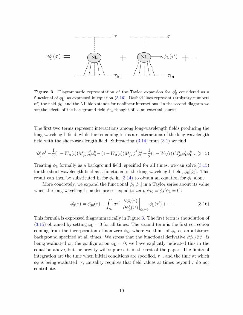
Figure 3. Diagrammatic representation of the Taylor expansion for φiS considered as a

functional of φjL, as expressed in equation (3.16). Dashed lines represent (arbitrary numbers

of) the field φS, and the NL blob stands for nonlinear interactions. In the second diagram we

see the effects of the background field φL, thought of as an external source.

The first two terms represent interactions among long-wavelength fields producing the

long-wavelength field, while the remaining terms are interactions of the long-wavelength

field with the short-wavelength field. Subtracting (3.14) from (3.1) we find

DijφjS−1

2(1−WΛ(i))M i

jkφjSφ

kS− (1−WΛ(i))M i

jkφjLφ

kS−

1

2(1−WΛ(i))M i

jkφjLφ

kL . (3.15)

Treating φL formally as a background field, specified for all times, we can solve (3.15)

for the short-wavelength field as a functional of the long-wavelength field, φS[φL]. This

result can then be substituted in for φS in (3.14) to obtain an equation for φL alone.

More concretely, we expand the functional φS[φL] in a Taylor series about its value

when the long-wavelength modes are set equal to zero, φS0 ≡ φS[φL = 0]:

φiS(τ) = φiS0(τ) +

∫ τ

τin

dτ ′∂φiS(τ)

∂φjL(τ ′)

∣∣∣∣φL=0

φjL(τ ′) + · · · (3.16)

This formula is expressed diagrammatically in Figure 3. The first term is the solution of

(3.15) obtained by setting φL = 0 for all times. The second term is the first correction

coming from the incorporation of non-zero φL, where we think of φL as an arbitrary

background specified at all times. We stress that the functional derivative ∂φS/∂φL is

being evaluated on the configuration φL = 0; we have explicitly indicated this in the

equation above, but for brevity will suppress it in the rest of the paper. The limits of

integration are the time when initial conditions are specified, τin, and the time at which

φS is being evaluated, τ ; causality requires that field values at times beyond τ do not

contribute.

– 10 –

Up to this point, we have assumed that the initial conditions at τin are completely

specified. For the application to LSS, however, we have a probability distribution over

initial conditions. For now we imagine selecting one particular initial condition from

the ensemble; the average over all possibilities is only taken at the very end of the

calculation. If instead we take the expectation value over the short-wavelength initial

conditions at this intermediate stage, we will miss some correlations. This effect may

become non-negligible at high orders in perturbation theory.

Returning to (3.14), we can plug in our perturbative expansion (3.16) to get

0 = DijφjL −1

2WΛ(i)M i

jkφjLφ

kL −WΛ(i)M i

jkφjS0φ

kL −

1

2WΛ(i)M i

jkφjS0φ

kS0

−WΛ(i)M ijkφ

jS0

∫ τ ∂φkS(τ)

∂φlL(τ ′)φlL(τ ′)−WΛ(i)M i

jkφjL

∫ τ ∂φkS(τ)

∂φlL(τ ′)φlL(τ ′) + · · · ,

(3.17)

where the · · · represent terms that, as we will see below, are higher order.

Notice that the induced interactions of the long-wavelength field with itself are non-

local in time. This is a very important conceptual point. The modes we have integrated

out are short-distance modes, but depending on the dynamics they may be long-lived.

This means that the functional derivative ∂φkS(τ)/∂φlL(τ ′) may have significant support

even when τ and τ ′ are very different. There are different possible strategies for dealing

with these terms. We will see below how they can be systematically accounted for in

perturbation theory. These interaction terms, and their perturbative forms, represent

the new parameters needed to define the EFT.

3.3 Effective Perturbation Theory

The next step, as in section 3.1 above, is to formally expand φL in a parameter ε and

use perturbation theory on this new, effective equation. We will assume that some

perturbative description is valid where φL ≈ φ(1) is still true to leading order (for the

long-wavelength modes), and so the new terms should only give corrections to that.

In order to make progress, we need to decide how many powers of ε to assign to the

new terms generated by interactions involving φS. This turns out to be an involved

question, and we will need to make use of some assumptions about the dynamics. For

concreteness, we will specifically refer to the theory of LSS.

The short-wavelength field φS is a complicated object. First consider φS0, the

solution for the short-wavelength perturbation in the absence of long-wavelength per-

turbations. For modes near the cutoff, the linear perturbation theory should still be

approximately valid and φS0 ≈ φ(1) should hold, so that φS0 ∼ ε. For the truly nonlin-

ear modes, we can no longer assume that φS0 is small. However, because perturbation

– 11 –

theory is still valid at long wavelengths, we will assume that the order of magnitude of

the effects of the modes at more nonlinear scales is well-estimated by the effects of the

modes at only slightly nonlinear scales. In other words, the scaling of the interaction

terms we get by assuming φS0 ∼ ε will be assumed to be the correct scaling. This

is an important assumption and we have not proved it. More detailed analyses of the

order-of-magnitude of nonlinear effects within the theory of LSS are performed in [2, 3].

There it is shown that the nonlinear effects are under control and that this estimation is

ultimately correct. However, this point may be an important restriction on the general

applicability of EFT methods to arbitrary equations of motion.

Similar comments can be made about the functional derivative ∂φS/∂φL. However,

at the level of the second derivative, ∂2φS/∂φ2L, there is a new effect. Because two long-

wavelength modes can come together to make a short-wavelength mode through the

interaction M , the second derivative ∂2φS/∂φ2L will have a term that does not contain

any factors of ε. A term in ∂2φS/∂φ2L with zero powers of ε thus acts at the same order

in perturbation theory as a term in ∂φS/∂φL with a single power of ε. This complicates

the perturbation expansion.

In the specific case of LSS, the origin of this complication is that the smoothing

procedure has removed too many modes from the theory. A short-wavelength mode

that is created from two long-wavelength modes, produced by the unsuppressed term

in ∂2φS/∂φ2L, is not a nonlinear mode. The reason is that short-wavelength modes

created in this way are nearly identical to long-wavelength modes created in the same

way: they are initially small (i.e., linear), and grow according to a k-independent linear

growth function. Like these long-wavelength modes, we expect short-wavelength modes

generated in this way to remain linear.

To summarize, in the expansion of φS there will be two types of terms. First, there

will be terms representing short-wavelength modes which have dynamically evolved

from short-wavelength initial conditions. We will assume that all such modes give O(ε)

contributions to φS and each of its functional derivatives. Second, there will be terms

representing short-wavelength modes which are generated through the action of the

background field φL alone. These terms do not represent nonlinear physics, and it is a

defect of the formalism that they appear here as modes to be smoothed over. We will

ignore these terms completely for now, even though they contribute non-ε-suppressed

contributions to the functional derivative. One reason why it is possible to ignore them

is because they make up only a small portion of the phase space at low order: when

only a few long-wavelength modes combine together to make a short-wavelength mode,

the resulting wavenumber will not be much greater than the cutoff Λ. At higher orders,

however, when there are more long-wavelength fields propagating, the numerical error

caused by a failure to systematically account for these modes will be greater. We leave

– 12 –

incorporation of these higher-order effects into this formalism for future work, although

we will have a bit more to say on the topic below when we discuss correlation functions.

In Section 4 below we present an alternative formalism that naturally takes these modes

into account.

We will now expand φL as a power series in ε, as we did with φ in (3.2). To make

the dependence on nonlinear effects explicit, we decompose each order in the expansion

into a “standard” piece and a piece generated by short-distance physics. We write

φiL = ε(φiL(1) + ∆φiL(1)) + ε2(φiL(2) + ∆φiL(2)) + ε3(φiL(3) + ∆φiL(3)) + · · · (3.18)

The functions φL(n) are defined to be the same as the φ(n) as in standard perturba-

tion theory, with the replacement M ijk → WΛ(i)M i

jk, and using the smoothed long-

wavelength initial conditions WΛ(i)φin instead of the unsmoothed initial conditions.

Equivalently, one could make the replacement Gij → WΛ(i)Gi

j, making use of the as-

sumption that G is diagonal in momentum. Physically, this means that only long-

wavelength fields are allowed to propagate in the construction of the φL(n). Diagram-

matically, all lines have their momenta cut off.

The effects of the short-wavelength interactions are denoted by ∆φL(n). We can find

equations of motion for the ∆φL terms by expanding the effective equation of motion

in ε. At O(ε) we find

Dij∆φjL(1) = 0 . (3.19)

Since the initial conditions are already accounted for in φL(1), the solution to this

equation is ∆φL(1) = 0. This is just a reflection of our assumption that the effects of

the short-distance scales on the long-distance scales can be treated perturbatively.

Using this result, we find at O(ε2)

Dij∆φjL(2) = WΛ(i)M ijkφ

jS0φ

kL(1) +

1

2WΛ(i)M i

jkφjS0φ

kS0 . (3.20)

Here we see the first effects of the short-distance physics. We can easily write down

the solution for ∆φiL(2) from this equation:

∆φiL(2)(τ) =

∫ τ

τin

dτ ′ Gij(τ ; τ ′)

[WΛ(j)M j

klφkS0φ

lL(1) +

1

2WΛ(j)M j

klφkS0φ

lS0

]. (3.21)

This solution is expressed diagrammatically in Figure 4.

At O(ε3) we have

Dij∆φjL(3) = WΛ(i)M ijkφ

jS0(φkL(2) +∆φkL(2))+WΛ(i)M i

jk(φjS0 +φjL(1))

∫ τ ∂φkS(τ)

∂φlL(τ ′)φlL(1)(τ

′) .

(3.22)

– 13 –

∆φiL(2)(τ) = +

τ

τin

τ

τin

NL NL NL

Figure 4. Diagrammatic representation of the solution for ∆φiL(2), as expressed in equa-

tion (3.21). Dashed lines are the short-wavelength field φS0, while solid lines are the long-

wavelength field φL. As in Figure 3, NL blobs represent nonlinear interactions.

Here at third order we find the first nonlocal-in-time interactions. However, in the

context of this perturbative expansion it is easy to deal with them. Since we already

know the full time-dependence of φL(1), we can factor it out of the time integral:∫ τ

τin

dτ ′∂φkS(τ)

∂φlL(τ ′)φlL(1)(τ

′) =

[∫ τ

τin

dτ ′∂φkS(τ)

∂φlL(τ ′)

[G(τ ; τ ′)−1

]lm

]φmL(1)(τ) . (3.23)

(The propagator is guaranteed to be invertible, because the equations of motion are

reversible.) Because perturbation theory is a recursive process, this procedure can

be repeated at each order. Then perturbatively the nonlocal-in-time interaction is

expressed in terms of local-in-time interactions. We can now write a simple expression

for ∆φL(3):

∆φiL(3)(τ) =

∫ τ

τin

dτ ′ Gij(τ ; τ ′)

[WΛ(j)M j

klφkS0

(φlL(2) + ∆φlL(2)

)+WΛ(j)M j

kl

(φkS0 + φkL(1)

) [∫ τ ′

τin

dτ ′′∂φlS(τ ′)

∂φmL (τ ′′)

[G(τ ′; τ ′′)−1

]mn

]φnL(1)(τ

′)

].

(3.24)

3.4 Correlation Functions

Using the formalism above we can compute correlation functions of the long-wavelength

field φL. The power spectrum in particular can be written as

〈φiLφjL〉 =〈φiL(1)φjL(1)〉+ 〈φiL(1)φ

jL(3)〉+ 〈φiL(3)φ

jL(1)〉+ 〈φiL(2)φ

jL(2)〉+ 〈φiL(1)∆φ

jL(3)〉

+ 〈∆φiL(3)φj(1)〉+ 〈φiL(2)∆φ

jL(2)〉+ 〈∆φiL(2)φ

jL(2)〉+ 〈∆φiL(2)∆φ

jL(2)〉+ · · · .

(3.25)

– 14 –

The first line is very similar to the 1-loop result from SPT, except every propagating

field is long-wavelength. The second line represents corrections to that result up to the

same order. Note that the sum of both lines is meant to be Λ-independent. In practice,

the Λ-dependence of the ∆φ terms is determined by this requirement since they cannot

be calculated from first principles. An example of such a calculation is performed in

Appendix A.

We note one technical point about this calculation. When computing the SPT-like

terms in the EFT expansion of the correlation function, every single field is supposed

to be restricted to being long-wavelength. In general, this will impose multiple different

cutoffs on each loop integral beyond those imposed by removing the short-wavelength

initial conditions, since some of the lines within the loop carry sums of other loop

momenta and the external momentum. This technical annoyance has, as far as we

are aware, gone unnoticed in the literature. The effects of such a restriction will be

small, subleading in kexternal/Λ for low orders in perturbation theory, but more impor-

tant at higher orders. This is related to the issue we mentioned above regarding the

contributions to φS which are not actually nonlinear. Those contributions precisely

correspond to lines in the loop diagram which go over the cutoff even when all initial

conditions are long-wavelength only. It would be preferable to have a formalism where

this was accounted for automatically, and the only cutoff that had to be performed on

the diagram was a cutoff on the initial conditions. This is achieved by the path integral

formalism discussed in the next section.

4 A Path Integral Approach

In this section we use a statistical path integral to incorporate the effects of the prob-

ability distribution over initial conditions on the equations of motion. By following

the Polchinski renormalization group procedure [15] we can deduce the structure of the

effective theory. Instead of smoothing the equations of motion, we will demand that

the coefficients in the effective action are closed under renormalization group flow. We

find general results that agree with the analysis of the previous section, up to the issues

relating to linear portions of φS discussed above, and offer new insight into the effective

theory.

4.1 Polchinski RG

In this section we review the usual equations of the Polchinski RG using our condensed

notation, where a Latin index is both a discrete label for field species and also a

– 15 –

continuous label for momentum. Consider an action of the form

S(φ,Λ) = −1

2φi[P (Λ)−1]ijφ

j + Sint(φ,Λ) , (4.1)

where P (Λ) is a symmetric matrix which depends on the momentum cutoff Λ.4 The

partition function,

Z =

∫Dφ eS , (4.2)

is a physical object and so should be independent of Λ, which was introduced artificially.

Taking the Λ-derivative gives

dZ

dΛ=

∫Dφ(−1

2φj

d

dΛ

[P (Λ)−1

]ijφj +

d

dΛSint(φ,Λ)

)eS . (4.3)

Then consider the quantity

∂

∂φi

(dP ij

dΛ[P−1]jkφ

keS +1

2

dP

dΛ

ij ∂S

∂φjeS)

=

(dP ij

dΛ[P−1]ji +

dP ij

dΛ[P−1]jkφ

k ∂S

∂φi+

1

2

dP

dΛ

ij ∂S

∂φj∂S

∂φi+

1

2

dP

dΛ

ij ∂2S

∂φi∂φj

)eS

=

(1

2

dP ij

dΛ[P−1]ji +

1

2φi

d

dΛ[P−1]ijφ

j +1

2

dP

dΛ

ij ∂Sint

∂φj∂Sint

∂φi+

1

2

dP

dΛ

ij ∂2Sint

∂φi∂φj

)eS .

(4.4)

Since this is a total derivative, it will vanish when (functionally) integrated with respect

to φ. Then, up to a field-independent but Λ-dependent shift in the action, the partition

function will be independent of Λ if

d

dΛSint(φ,Λ) = −1

2

(dP

dΛ

ij ∂Sint

∂φj∂Sint

∂φi+dP

dΛ

ij ∂2Sint

∂φi∂φj

). (4.5)

We have neglected the appearance of an external current in the free action, but the

current drops out of the final equation if it is chosen to be orthogonal to dP/dΛ:

dP ij

dΛJj = 0 . (4.6)

Since dP/dΛ only has support near the cutoff Λ, this is usually guaranteed by choosing

J to have support only at low momentum.

4P should be thought of as a smoothly-varying function of momentum k and the cutoff Λ which is

Λ-independent when k < Λ and zero when k > Λ, and transitions rapidly between these two phases

for k ∼ Λ. In the EFT of LSS, P is the smoothed initial power spectrum.

– 16 –

We can expand the interaction as a power series:

Sint =∞∑m=0

1

m!Vi1···im(Λ)φi1 · · ·φim . (4.7)

Then we have the identities

∂Sint

∂φi=

∞∑m=0

1

m!Vii1···im(Λ)φi1 · · ·φim , (4.8)

∂2Sint

∂φi∂φj=

∞∑m=0

1

m!Viji1···im(Λ)φi1 · · ·φim . (4.9)

The RG equation (4.5) can be written in terms of the V coefficients as

d

dΛVi1···im(Λ) = −1

2

(dP

dΛ

ij

Viji1···im +dP

dΛ

ij m∑k=0

(m

k

)Vii1···ikVjik+1···im

). (4.10)

There is a simple diagrammatic interpretation to this equation. The LHS represents a

vertex with m external legs. The first term on the RHS is a vertex with m+ 2 external

legs, and two of them are contracted with the free propagator. The second term on the

RHS takes a vertex with k+ 1 external lines and another with m− k+ 1 external lines

and connects them by contracting one line from each vertex using a propagator.

4.2 A Path Integral for Standard Perturbation Theory

In cosmological perturbation theory we are given initial data φiin at the initial time τin

for some collection of perturbation fields. For simplicity, we will assume that these

satisfy Gaussian statistics, meaning that their correlation functions can be calculated

using the path integral

〈φi1in · · ·φinin 〉 =

∫Dφin φ

i1in · · ·φinin exp

(−1

2φiin[P−1

in ]ijφjin

). (4.11)

This is a three-dimensional Euclidean path integral over the set of all initial pertur-

bation configurations. The matrix Pin appearing here is the initial power spectrum.

Of course, in reality there will be a small amount of non-Gaussianity in the statistics

at τin, coming from nonlinear evolution prior to τin in addition to possible primordial

non-Gaussianity. To account for this we can replace the exponent in (4.11) with a more

complicated functional of the φin, including higher order terms.

We can use this same path integral to compute the correlation functions of the

perturbations at a later time as well. Denote these late-time perturbations by φi,

– 17 –

suppressing reference to the time of evaluation τ0. The procedure is simply to write the

late-time perturbations as functionals of the initial data, φi = φi[φin], computed from

the equations of motion, and then plug this into the path integral:

〈φi1 · · ·φin〉 =

∫Dφin φ

i1 [φin] · · ·φin [φin]eS0[φin] . (4.12)

The “free action” S0 is just the same quantity which appeared in the exponent of (4.11).

The late-time correlation functions can be collected into a generating functional Z[J ]:

Z[J ] =

∫Dφin exp

(S0[φin] + Jiφ

i[φin]). (4.13)

Now we note that the external current term in the exponential can be alternatively

interpreted as a complicated interaction term for φin. By solving for φi in perturbation

theory, we obtain a polynomial expansion for the interactions, the vertices of which are

determined by integrating the equations of motion perturbatively. In SPT, we have a

natural expansion for φi:

φiSPT ≡ KiSPT j φ

jin +

1

2Ki

SPT jk φjinφ

kin + · · · . (4.14)

In the notation of the previous section, we would write

φj(m) =1

m!Kj

SPT i1···im φi1in . . . φ

imin . (4.15)

Comparison to equations (3.3) and (3.4) leads to explicit formulas for KiSPT j and

KiSPT jk:

KiSPT j = Gi

j(τ0; τin) , (4.16)

KiSPT jk =

∫ τ0

τin

dτ ′ Gin(τ0; τ ′)Mn

lmGlj(τ′; τin)Gm

k (τ ′; τin) . (4.17)

The higher order coefficients can be computed analogously. Using these, that the m-

point interaction vertex for φin is given by

VSPT i1···im ≡ JjKjSPT i1···im . (4.18)

4.3 RG in the Effective Theory

We will now introduce a cutoff to the theory. First, we replace the initial power

spectrum with the smoothed power spectrum in the free part of the action: P ijin →

WΛ(i)2P ijin ≡ P ij. For this section, WΛ is a function which is equal to 1 for k . Λ, has a

– 18 –

non-vanishing derivative for k ∼ Λ, and then is equal to 0 for k & Λ. With this choice,

dP/dΛ is only nonzero over a very small range of momenta right near the cutoff. In

this way we have restricted the set of possible initial conditions for the perturbations.

Second, we restrict the external current J to have support only for modes k < Λ.

It is important that the support of J be distinct from the support of dP/dΛ. This

corresponds to only allowing ourselves to ask questions about long-wavelength modes.

Having made these restrictions, we need to include additional Λ-dependent inter-

action terms which incorporate the effects of the UV modes that have been eliminated.

We will deduce the form of these interactions by demanding that the full set is closed

under the RG flow, 4.10. There are three classes of new terms, two of which we have

already discussed. First, there are terms linear in J , which represent propagation. Sec-

ond, there are terms which are J-independent and represent renormalizations of the

effective initial power spectrum, as well as induced initial non-Gaussianities. The third

class of terms, which we have not yet discussed, contains the terms nonlinear in J .

Normally, terms with higher powers of an external current are not generated by RG

evolution. This is because the external current is chosen to have support only over

momenta for which dP/dΛ = 0, and so J drops out of the RG equations as discussed

above near (4.6). However, that is not the case here. Consider the contraction of the

m-point interaction with dP/dΛ, as it occurs in (4.10):

dP ii1

dΛVSPT i1···im =

dP ii1

dΛJjK

jSPT i1···im(q1, · · · , qm) . (4.19)

To make things a little more clear, we will restore explicit momentum dependence to

this equation and use conservation of momentum to simplify the expression. Then, by

a slight abuse of notation, we have

dP ii1

dΛ(q1)VSPT i1···im(q1, · · · , qm) =

∫d3q1

(2π)3

dP ii1

dΛ(q1)Jj

(−∑

qi

)Kj

SPT i1···im(q1, · · · , qm) .

(4.20)

The power spectrum derivative is only nonzero when q1 ≈ Λ, and J vanishes unless∑qi < Λ. Except for m = 1, these requirements can be simultaneously satisfied.

Therefore J does not drop out of the RG equations. Hence RG evolution is nonlinear,

and we will generate terms which are nonlinear in J . These are generalized evolution

terms for φ; heuristically, they encode the effects of the stochastic source terms of the

precious section.

In general, we can write a series expansion for the fullm-point interaction coefficient

V :

Vi1···im =∞∑n=0

1

n!Jj1 · · · JjnKj1···jn

i1···im . (4.21)

– 19 –

=d

dΛ +

Figure 5. Diagrammatic representation of the renormalization group equation (4.22). The

curved bracket at the bottom represents a contraction with a factor of dP ij/dΛ. The second

graph on the right stands for a sum over various ways to distribute and contract the incoming

lines.

The n = 0 and n = 1 terms are the renormalized initial distribution function and

standard time evolution, respectively, while the n > 1 terms are the new ones. We can

expand (4.10) as a power series in J to obtain RG equations for the K coefficients.

This yields

d

dΛKj1···jni1···im = −1

2

(dP

dΛ

ij

Kj1···jniji1···im +

dP

dΛ

ij m∑k=0

n∑l=0

(m

k

)(n

l

)Kj1···jlii1···ikK

jl+1···jnjik+1···im

). (4.22)

Since the RHS of (4.22) involves only terms with ≤ n raised indices, the equations

can be solved order-by-order in n. The n = 0 terms therefore renormalize among

themselves. We immediately learn that if all n = 0 terms vanish, non-zero terms will

never be generated by the RG. This means that a Gaussian initial distribution at all

scales, and the power spectrum is unchanged.

Now we examine the n = 1 equation:

d

dΛKj1i1···im = −1

2

dP

dΛ

ij[Kj1iji1···im +

m∑k=0

(m

k

)(Kj1ii1···ikKjik+1···im +Kii1···ikK

j1jik+1···im

)].

(4.23)

If the initial perturbations are Gaussian, K coefficients with zero upper indices vanish,

so the first term on the RHS is the only one that survives. For the special case m = 1,

we findd

dΛKj1i1

= −1

2

dP

dΛ

ij

Kj1iji1

. (4.24)

– 20 –

Since K coefficients with a single upper index correspond to renormalized time evo-

lution, we can write K = KSPT + ∆K for these, where KSPT is defined above and is

independent of Λ. Then we have

d

dΛ∆K l

m = −1

2

dP

dΛ

ij

(K lSPT ijm + ∆K l

ijm) . (4.25)

The ∆K factors are only nonzero because they are generated by this equation. There-

fore they are suppressed relative to the KSPT factors by P ij. To the extent that per-

turbation theory is valid, this means they are small.

The utility of this equation will be more recognizable if we compute 〈φn(1)φm(3)〉Λ

in the notation of this section, where the subscript Λ means that we take the SPT

calculation and restrict the initial conditions to be long-wavelength:

〈φn(1)φm(3)〉Λ =

1

6Km

SPT jkl

(〈φn(1)φ

jin〉Λ〈φkinφlin〉Λ + 〈φn(1)φ

kin〉Λ〈φjinφlin〉Λ + 〈φn(1)φ

lin〉Λ〈φjinφkin〉Λ

)(4.26)

=1

6Km

SPT jkl

(〈φn(1)φ

jin〉ΛP kl + 〈φn(1)φ

kin〉ΛP jl + 〈φn(1)φ

lin〉ΛP jk

)(4.27)

=1

2Km

SPT jkl〈φn(1)φlin〉ΛP jk (4.28)

=1

2Km

SPT jkl〈φn(1)φlin〉P jk . (4.29)

In the last equality we have used the fact that the momentum associated with the n

index is below the cutoff, so 〈φn(1)φlin〉Λ is actually independent of Λ. Then all of the

Λ-dependence of this expression is in the P jk factor. Taking the Λ-derivative and using

(4.25) we find

d

dΛ〈φn(1)φ

m(3)〉Λ =

1

2Km

SPT jkl〈φn(1)φlin〉dP

dΛ

jk

(4.30)

= −〈φn(1)φlin〉(d

dΛ∆Km

l +dP

dΛ

jk 1

2∆Km

jkl

)(4.31)

= − d

dΛ

(〈φn(1)∆K

ml φ

lin〉)− 1

2∆Km

jkl〈φn(1)φlin〉dP

dΛ

jk

(4.32)

Since the ∆K terms are small in perturbation theory, the second term on the RHS can

be dropped as it is subdominant compared to the first term. Then this equation says

that the Λ-dependence of 〈φn(1)φm(3)〉 is canceled by Λ dependence of 〈φn(1)∆φ

m(3)〉, where

∆φm(3) = ∆Kml φ

lin. We can think of this as a renormalization of the propagation of φ.

It is tempting to identify this correction with ∆φL(3) from Section 3, but they

are not the same. Recall that ∆φL(3) was defined as the correction to φL(3), which was

– 21 –

related to φ(3) be restricting every propagating state to be long-wavelength. Here we are

not doing that. We are only restricting the initial conditions to be long-wavelength,

but these may generate short-wavelength states spontaneously. The spontaneously

generated short-wavelength states remain linear, as discussed in Section 3, and so they

are automatically incorporated in SPT. The correction ∆φ(3) of the present section is

the correction to the SPT result (with restricted initial conditions), and so does not

include these particular modes.

Now we turn to the n = 2 equation, which represents the simplest type of general-

ized evolution. In that case we have

d

dΛKj1j2i1···im = −1

2

(dP

dΛ

ij

Kj1j2iji1···im +

dP

dΛ

ij m∑k=0

2∑l=0

(m

k

)(2

l

)Kj1···jlii1···ikK

jl+1···j2jik+1···im

). (4.33)

The first term on the RHS is a generalized evolution term, and so will be subleading

compared to terms in the sum which are not suppressed by the power spectrum. If

the initial perturbations are Gaussian, the l = 0 and l = 2 terms in the sum on the

RHS vanish. The remaining sum over k vanishes for m = 0 and m = 1 by momentum

conservation and orthogonality of J and dP/dΛ. The simplest nontrivial case is m = 2,

where we find the equation reduces to

d

dΛKj1j2i1i2

= −1

2

(dP

dΛ

ij

Kj1j2iji1i2

+ 4dP

dΛ

ij

Kj1ii1Kj2ji2

). (4.34)

To leading order in perturbation theory, this equation is

d

dΛKj1j2i1i2

= −2dP

dΛ

ij

Kj1SPT ii1

Kj2SPT ji2

(4.35)

The meaning of this equation can be illuminated by considering 〈φn(2)φm(2)〉Λ:

〈φn(2)φm(2)〉Λ =

1

4Kn

SPT ijKmSPT kl

(〈φiinφjin〉Λ〈φkinφlin〉Λ + 〈φiinφkin〉Λ〈φjinφlin〉Λ + 〈φiinφlin〉Λ〈φkinφjin〉Λ

)(4.36)

=1

4Kn

SPT ijKmSPT kl

(P ijP kl + P ikP jl + P ilP kj

)(4.37)

=1

2Kn

SPT ijKmSPT klP

ikP jl + 〈φn(2)〉Λ〈φm(2)〉Λ . (4.38)

The second term vanishes in the theory of LSS based on the explicit form of KSPT, which

we can see in Appendix A. To leading order in perturbation theory, the Λ-derivative of

– 22 –

the first term is

d

dΛ〈φn(2)φ

m(2)〉Λ = Kn

SPT ijKmSPT klP

ik dP

dΛ

jl

(4.39)

= −1

2P ik d

dΛKnmik (4.40)

= −1

2

d

dΛ

(P ikKnm

ik

)+

1

2

dP

dΛ

ik

Knmik (4.41)

= −1

2

d

dΛ

(P ikKnm

ik + 2Knm). (4.42)

In the last line we have used another of the RG equations. Notice that the 〈φ(2)φ(2)〉Λcontribution to the correlation function has its Λ-dependence canceled by new types

of terms not present in the classical theory. The second term, in particular, is strange

because it has no lowered indices. That means it comes from a field-independent (but

J-dependent) interaction in the effective action.

Let us take a moment to examine the RG equation associated with such terms:

d

dΛKj1···jn = −1

2

(dP

dΛ

ij

Kj1···jnij +

dP

dΛ

ij n∑l=0

(n

l

)Kj1···jli K

jl+1···jnj

). (4.43)

We will restrict our attention to n = 1 and n = 2, since those are the terms which are

relevant for the one- and two-point functions, and for simplicity we continue to assume

a Gaussian initial power spectrum. For n = 1, the equation becomes

d

dΛKj1 = −1

2

dP

dΛ

ij

Kj1ij . (4.44)

We can once more write Kj1ij = Kj1

SPT ij + ∆Kj1ij . In the theory of LSS, the term with

KSPT vanishes due to momentum conservation and the explicit form of KSPT. Therefore

the only contribution is from ∆Kj1ij . So Kj1 is suppressed by two powers of P ij.

Now we turn to n = 2:

d

dΛKj1j2 = −1

2

(dP

dΛ

ij

Kj1j2ij + 2

dP

dΛ

ij

Kj1i K

j2j

). (4.45)

The second term actually vanishes by momentum conservation and the orthogonality

of dP/dΛ and J . Then Kj1j2 is also generated at second order in P .

4.4 Renormalization of the One-Point Function and Power Spectrum

We can use the above formalism to compute the one-point function and two-point

function by taking derivatives of Z. The first derivative of Z is

∂Z

∂Ji= Z[J ]

∞∑m=0

∞∑n=0

1

m!n!Jj1 · · · JjnKij1···jn

i1···im 〈φi1in · · ·φimin 〉JΛ , (4.46)

– 23 –

where 〈· · · 〉JΛ denotes the expectation value in the presence of nonzero J (as well as the

cutoff Λ). This means that the expectation value of φ is

〈φi〉Λ =1

Z[0]

∂Z

∂Ji

∣∣∣∣J=0

=∞∑m=0

1

m!Kii1···im〈φ

i1in · · ·φimin 〉Λ . (4.47)

None of the nonlinear terms in J are involved in this computation. Generally speaking,

the n-point function requires knowledge of the Jk terms in the action for k ≤ n. So

the one-point function is based purely on the renormalized evolution defined by the

interaction terms linear in J . Also note that all of these expectation values are taken

with J = 0, so that they are Gaussian expectation values if the initial distribution is

Gaussian, using the cut-off initial power spectrum WΛ(i)2P ijin . In this special case, only

the even terms in (4.47) are nonvanishing.

To compute the two-point function, we take another derivative of (4.46), divide by

Z, and set J = 0:

〈φiφj〉Λ =1

Z[0]

∂2Z

∂Ji∂Jj

∣∣∣∣J=0

=∞∑m=0

m∑k=0

1

m!

(m

k

)Kii1···ikK

jik+1···im〈φ

i1in · · ·φimin 〉Λ

+∞∑m=0

1

m!Kiji1···im〈φ

i1in · · ·φimin 〉Λ + 〈φi〉Λ〈φj〉Λ .

(4.48)

The third term is the disconnected piece, and the first term is the answer one would

expect if the effective theory simply consisted of renormalized classical propagation of

φ, while the second term is the generalized evolution.

For simplicity, let us set the disconnected piece to zero and assume Gaussian initial

perturbations. Then up to second order in P ij we have

〈φiφj〉 = 〈φi(1)φj(1)〉+

[〈φi(1)φ

j(3)〉Λ + 〈φi(1)∆K

jk φ

kin〉Λ + (i↔ j)

]+

[〈φi(2)φ

j(2)〉Λ +Kij +

1

2Kiji1i2P i1i2

].

(4.49)

The first term is the linear evolution, and is Λ-independent. The bracketed collections

of terms are each Λ-independent at this order in perturbation theory based on the

analysis above. This expression can be compared with (3.7) in standard perturbation

theory, or (3.25) in the smoothing formalism.

Our analysis of the path integral has been fairly formal, but nevertheless extremely

instructive. This approach to cosmological perturbation theory reveals which collec-

tions of terms must have vanishing Λ-dependence, as well as indicating what kinds of

– 24 –

structures are generated by renormalization. It is also able to automatically incorpo-

rate the effects of short-wavelength modes that are generated by interactions of the

long-wavelength modes (and are therefore in the linear regime). The appearance of

integration kernels K with multiple upper indices is novel, representing effects directly

attributable to these generated short-wavelength modes. It would be interesting to

connect these with the statistics of a stochastic source term in the equations of motion.

5 Conclusions and Further Directions

The application of effective field theory ideas to the evolution of large-scale structure

involves a number of subtle issues. Unlike in quantum field theory, here the underlying

model is a classical field theory with probabilistic initial conditions, in which modes at

all wavelengths can propagate over large distances. Fortunately, in the real world it

is short-wavelength modes that are nonlinear, allowing us to construct a perturbation

theory for the long-wavelength modes.

In this paper we analyzed two methods of deriving such a theory. The first ap-

proach, which proceeds by smoothing the fields, most closely resembles previous work

in the subject. We were able to carefully derive consistent expressions for the long-

wavelength modes by first expressing the short-wavelength parts as a Taylor expansion

in the long-wavelength background. This makes the dependence on nonlinear effects

very explicit. There is a technical speed bump inherent in this technique, however, due

to the ability of interactions between long-wavelength modes to create perturbative

short-wavelength modes, which the smoothing procedure automatically squelches.

Our other method starts with a path integral over initial perturbations, and uses

the renormalization group to derive conditions obeyed by correlation functions. This

approach is quite general and flexible, and naturally accounts for the effects of perturba-

tive short-wavelength modes. Further investigation will be required to see how practical

this technique is for calculations beyond what is shown in Appendix A (although we

see no reason why it shouldn’t be).

The main open question is that of predictivity. In both methods a huge number

of effective interactions are generated. Much of the power of EFT as used in quantum

field theory comes from the reduction of the possible number of terms due to symme-

tries. It has been argued in [2, 3] that only a certain collection of terms are present in

the effective theory. However, it is not yet clear in the formalisms we discuss precisely

how the symmetries act to simplify the equations. In particular, the nonlocal-in-time

interactions of the smoothed picture are qualitatively different from the types of inter-

actions we are used to considering, and further study may illuminate some unexpected

properties.

– 25 –

Acknowledgments

We thank Clifford Cheung and Mark Wise for helpful conversations. This research

is funded in part by DOE grant No. DE-FG02-92ER40701, and by the Gordon and

Betty Moore Foundation through Grant No. 776 to the Caltech Moore Center for

Theoretical Cosmology and Physics. The work of SL is supported by a John A. McCone

Postdoctoral Fellowship.

A Explicit Calculations

In this appendix we perform some explicit calculations in both SPT and the EFT of

LSS in a simple setting. We will use a single-component, nonrelativistic, rotation-free

dark matter fluid moving in an Einstein-de Sitter background, subject to Newtonian

gravitational attraction. Extensions to multi-component fluids and the full theory of

general relativity are straightforward, but distracting. All of the fundamental concep-

tual issues are present already in this simple calculation.

A.1 Standard Perturbation Theory

In an Einstein-de Sitter cosmology—that is, a flat, matter-dominated FRW universe—

the scale factor is given by a(τ) = (τ/τ0)2, the conformal Hubble factor is H =

a−1da/dτ = 2/τ , and the equations of motion for a dark matter fluid simplify to

0 = ∂τδ(τ,k) + θ(τ,k) +

∫d3q

(2π)3

k · qq2

δ(τ,k− q)θ(τ,q) , (A.1)

0 = ∂τθ(τ,k) +Hθ(τ,k) +3

2H2δ(τ,k) +

∫d3q

(2π)3

k2q · (k− q)

2q2(k− q)2θ(τ,k− q)θ(τ,q).

(A.2)

At first order, we drop the nonlinear terms and solve the linearized equations using

a Green function: δ(1)(τ,k)

θ(1)(τ,k)

= G(τ ; τin)

δin(k)

θin(k)

. (A.3)

Here δin and θin are initial conditions at the initial time τin, and G(τ, τin) is a retarded

Green function for the linearized system:

G(τ1; τ2) =

3τ51 +2τ525τ31 τ

22

−τ51 +τ525τ31 τ2

−6(τ51−τ52 )

5τ41 τ22

2τ51 +3τ525τ41 τ2

Θ(τ1 − τ2). (A.4)

– 26 –

Note that for τ � τin we have δ(1) ∝ τ 2 ∝ a, which is the dominant growth function

behavior familiar from standard perturbation theory. By keeping careful track of both

θ and δ we are effectively including the subdominant mode as well.

The method of SPT is to incorporate nonlinearities perturbatively by substituting

the linear solution into the nonlinear terms and treating them as a source for the

second-order terms. Then we haveδ(2)(τ,k)

θ(2)(τ,k)

= −∫ τ

τin

dτ ′∫

d3q

(2π)3G(τ ; τ ′)

k·qq2δ(1)(τ

′,k− q)θ(1)(τ′,q)

k2q·(k−q)2q2(k−q)2

θ(1)(τ′,k− q)θ(1)(τ

′,q)

.

(A.5)

This procedure can be repeated to compute higher-order perturbations. For instance,

at the next order we haveδ(3)(τ,k)

θ(3)(τ,k)

=−∫ τ

τin

dτ ′∫

d3q

(2π)3G(τ ; τ ′)

×

k·qq2

[δ(1)(τ

′,k− q)θ(2)(τ′,q) + δ(2)(τ

′,k− q)θ(1)(τ′,q)

]k2q·(k−q)q2(k−q)2

θ(1)(τ′,k− q)θ(2)(τ

′,q)

.

(A.6)

The expansion is tedious but straightforward to compute.

Before continuing, it will be useful to make contact with the notation of the body of

the paper. The perturbations δ and θ are regarded as components of the perturbation

field φi, where i = δ or i = θ (for added clarity we label the momentum separately, and

not as part of the Latin index). Then (A.3) can be replaced by

φi(1)(τ,k) = Gij(τ ; τin)φjin(k) . (A.7)

The nonlinear terms in the equations of motion can be incorporated into the pair of

matrices

M δij(k1; k2,k3) =

0 −k1·k3

k23

−k1·k2

k220

, (A.8)

M θij(k1; k2,k3) =

0 0

0 −k21(k2·k3)

k22k23

, (A.9)

– 27 –

so that (A.5) and (A.6) become, respectively,

φi(2)(τ,k) =1

2

∫ τ

τin

dτ ′∫

d3q

(2π)3Gij(τ ; τ ′)M j

lm(k; k− q,q)φl(1)(τ′,k− q)φm(1)(τ

′,q) ,

(A.10)

and

φi(3)(τ,k) =

∫ τ

τin

dτ ′∫

d3q

(2π)3Gij(τ ; τ ′)M j

lm(k; k−q,q)φl(1)(τ′,k−q)φm(2)(τ

′,q) . (A.11)

The correlation function we will use as our example is

〈φi(1)(τ1,k1)φj(3)(τ2,k2)〉 , (A.12)

which occurs in the SPT expansion of

〈φi(τ1,k1)φj(τ2,k2)〉 . (A.13)

We just have to multiply φ(1) and φ(3) above and take the expectation value using

Wick’s theorem (assuming Gaussian initial conditions). The result will depend on the

linear power spectrum

〈φi(1)(τ1,k1)φj(1)(τ2,k2)〉 ≡ P ij(11)(τ1, τ2|k1)(2π)3δ(3)(k1 + k2) . (A.14)

The presence of the Dirac δ-function is a result of translation invariance, and in addition

rotational invariance implies that P ij(11)(k) is a function only of k2. These results produce

numerous simplifications, in particular that 〈φi(2)〉 = 0. Doing a little algebra, we find

that

〈φi(1)(τ1,k1)φj(3)(τ2,k2)〉 = (2π)3δ(3)(k1 + k2)

∫ τ2

τin

dτ ′∫ τ ′

τin

dτ ′′∫

d3q

(2π)3Gjk(τ2; τ ′)

Mklm(k2; q,k2 − q)Gm

n (τ ′; τ ′′)Mnop(k2 − q;−q,k2)P ip

(11)(τ1, τ′′|k1)P lo

(11)(τ′, τ ′′|q) .

(A.15)

The overall factor of (2π)3δ(3)(k1 + k2) is present because translation invariance is

respected at each order in perturbation theory. Here q is the loop momentum, which

still must be integrated over.

A.2 Accounting for the Cutoff

Now we will discuss the two approaches to regulating 〈φ(1)φ(3)〉, before discussing how

the Λ-dependence of the result is canceled by new interactions. First, the smoothing

– 28 –

method of Section 3 demands that we replace φ(1) and φ(3) with φL(1) and φL(3). The

result is

〈φiL(1)(τ1,k1)φjL(3)(τ2,k2)〉 = (2π)3δ(3)(k1 + k2)

×∫ τ2

τin

dτ ′∫ τ ′

τin

dτ ′′∫

d3q

(2π)3

[Gjk(τ2; τ ′)WΛ(k2)Mk

lm(k2; q,k2 − q)Gmn (τ ′; τ ′′)

×WΛ(|k2 − q|)Mnop(k2 − q;−q,k2)WΛ(k1)2P ip

(11)(τ1, τ′′|k1)WΛ(q)2P lo

(11)(τ′, τ ′′|q)

].

(A.16)

Notice that there are two nontrivial constraints on the loop integral. The two con-

straints |k2 − q| < Λ and q < Λ are awkward to satisfy simultaneously. However, if we

ignore the constraint on |k2 − q| then we only make an error of order k2/Λ, which is

small for us.

The alternative approach is the RG path integral of Section 4. There we are

instructed to only place a cutoff on the initial conditions:

〈φi(1)(τ1,k1)φj(3)(τ2,k2)〉Λ = (2π)3δ(3)(k1 + k2)×∫ τ2

τin

dτ ′∫ τ ′

τin

dτ ′′∫

d3q

(2π)3

[Gjk(τ2; τ ′)Mk

lm(k2; q,k2 − q)Gmn (τ ′; τ ′′)×

Mnop(k2 − q;−q,k2)WΛ(k1)2P ip

(11)(τ1, τ′′|k1)WΛ(q)2P lo

(11)(τ′, τ ′′|q)

].

(A.17)

Unlike the smoothing prescription, here do not place a bound on |k2 − q|. The other

difference is a missing factor of WΛ(k2), but this factor is redundant since k2 is an

external momentum which must be small. This integral is more straightforward to

compute, but, as mentioned above, until we are ready to compute to the level of k2/Λ

precision there is no real difference. Either computation is well-approximated by (A.15)

with a hard momentum cutoff at q = Λ.

We continue the calculation be performing the angular part of the integral over q

in (A.15). Defining the matrix Σ by

Σkp(τ′; τ ′′|k) =

∫d3q

(2π)3Mk

lm(k; q,k− q)Gmn (τ ′; τ ′′)Mn

op(k− q;−q,k)P lo(11)(τ

′, τ ′′|q) ,(A.18)

we have

Σkp(τ′; τ ′′|k) =

k3

4π

∫dr

[−2

3P θθ

(11)(τ′, τ ′′|kr)Gk

p(τ′; τ ′′) +

1

2Gθδ(τ′; τ ′′)Πk

p

], (A.19)

– 29 –

where q ≡ kr. The entries of the Π matrix are

Πδδ =

(1 + r2 +

1

4r

(1− r2

)2log

(1− r)2

(1 + r)2

)P δθ

(11)(τ′, τ ′′|kr) , (A.20)

Πδθ = −

(−5

3r2 + r4 +

r

4

(1− r2

)2log

(1− r)2

(1 + r)2

)P δδ

(11)(τ′, τ ′′|kr) , (A.21)

Πθδ =

(r−2 − 5

3+

1

4r3

(1− r2

)2log

(1− r)2

(1 + r)2

)P θθ

(11)(τ′, τ ′′|kr) , (A.22)

Πθθ = −

(1 + r2 +

1

4r

(1− r2

)2log

(1− r)2

(1 + r)2

)P θδ

(11)(τ′, τ ′′|kr) . (A.23)

Hence (A.15) can be rewritten succinctly as

〈φi(1)(τ1,k)φj(3)(τ2,−k)〉′ =∫ τ

τin

dτ ′∫ τ ′

τin

dτ ′′ Gjk(τ2; τ ′)Σk

p(τ′; τ ′′|k)P ip

(11)(τ1, τ′′|k) .

(A.24)

Here the ′ means that we have dropped the overall δ-function. In an Einstein-de Sitter

universe, we can use (A.4) to do the time integrations analytically. The result is simple

in the limit τ1 = τ2 ≡ τ � τin if we also isolate the large r part of (A.20-A.23). We

find that

〈φi(1)(τ,k)φj(3)(τ,−k)〉′ ≈ 1

5

k2

4π2

−6163

6163H

3H −3H2

P δδ(11)(τ, τ |k)

∫q�k

dq P δδ(11)(τ, τ |q) .

(A.25)

It is at this point that we introduce a cutoff Λ in the integral over q. Approximating

this integral by the contribution for q near Λ is valid up to corrections of order k/Λ.

The Λ-dependence of this correlation function needs to be canceled against the

Λ-dependence of either 〈φiL(1)∆φjL(3)〉 or 〈φi(1)∆K

jk φ

kin〉Λ, depending on which approach

we use. In this case, to the level of approximation to which we are working, they are

the same. We will use the smoothing picture here because it gives us more information.

The formal expression for ∆φiL(3) is (3.24), which has several terms featuring different

combinations of short and long wavelength fields.

When we look at the expectation value 〈φiL(1)∆φjL(3)〉 there are some simplifications

due to momentum conservation and Gaussian statistics. Because of Gaussian statistics,

the expectation value reduces to a sum of products of pairs of expectation values.

Because of momentum conservation, the long-wavelength fields can only be paired

with the long-wavelength fields. Therefore terms with an odd number of φL(1) factors

when fully expanded will vanish. After some algebra, this leaves us with

〈φiL(1)∆φjL(3)〉 = 〈φi(1)∆K

jkφ

kin〉Λ , (A.26)

– 30 –

where

∆Kjk =

∫ τ

τin

dτ ′∫ τ ′

τin

dτ ′′ Gjp(τ ; τ ′)Mp

lmφlS0

[Gmn (τ ′; τ ′′)Mn

opφpS0 +

∂φmS (τ ′)

∂φoL(τ ′′)

]Gok(τ′′, τin) .

(A.27)

We see that the form of the correction is identical to what was expected based on the

analysis from Section 4. Alternatively, we can write this correction as

〈φiL(1)∆φjL(3)〉′ =

∫ τ

τin

dτ ′ Gjk(τ ; τ ′)Ck

l (τ ′|k)P il(11)(τ, τ

′|k) , (A.28)

with

Ckl (τ ′|k) =

∫ τ ′

τin

dτ ′′ Mkqmφ

qS0

(Gmn (τ ′; τ ′′)Mn

opφpS0 +

∂φmS (τ ′)

∂φoL(τ ′′)

)[G(τ ′; τ ′′)−1

]ol. (A.29)

In perturbation theory, this is same result as one would have gotten from a term

Ckl (τ ′|k)φl(k) (A.30)

added to the equation of motion for φ.

In the theory of LSS, it has been argued [1, 2] that the terms one should add to

the equations of motion represent the parameters of an imperfect fluid. In particular,

to lowest order in k/Λ, the coefficients of the C matrix determine the sound speed,

viscosity, and heat conduction coefficients in the fluid:

C(τ |k) =

χδ χθ

k2c2s −k2 c

2v

H

. (A.31)

These four coefficients are expected on the basis of thermodynamic considerations. We

should note that the Λ-dependence of (A.25) cannot be fully accounted for with the

sound speed and viscosity coefficients, c2s and c2

v alone. Nonzero heat conduction terms

are also required. This agrees with the recent result of [6].

References

[1] D. Baumann, A. Nicolis, L. Senatore, and M. Zaldarriaga, “Cosmological

Non-Linearities as an Effective Fluid,” JCAP 1207 (2012) 051, arXiv:1004.2488

[astro-ph.CO].

[2] J. J. M. Carrasco, M. P. Hertzberg, and L. Senatore, “The Effective Field Theory of

Cosmological Large Scale Structures,” JHEP 1209 (2012) 082, arXiv:1206.2926

[astro-ph.CO].

– 31 –

[3] M. P. Hertzberg, “The Effective Field Theory of Dark Matter and Structure

Formation: Semi-Analytical Results,” arXiv:1208.0839 [astro-ph.CO].

[4] E. Pajer and M. Zaldarriaga, “On the Renormalization of the Effective Field Theory of

Large Scale Structures,” JCAP 1308 (2013) 037, arXiv:1301.7182 [astro-ph.CO].

[5] J. J. M. Carrasco, S. Foreman, D. Green, and L. Senatore, “The 2-loop matter power

spectrum and the IR-safe integrand,” arXiv:1304.4946 [astro-ph.CO].

[6] L. Mercolli and E. Pajer, “On the Velocity in the Effective Field Theory of Large Scale

Structures,” arXiv:1307.3220 [astro-ph.CO].

[7] J. J. M. Carrasco, S. Foreman, D. Green, and L. Senatore, “The Effective Field Theory

of Large Scale Structures at Two Loops,” arXiv:1310.0464 [astro-ph.CO].

[8] J. N. Fry, “The Galaxy correlation hierarchy in perturbation theory,” Astrophys.J. 279

(1984) 499–510.

[9] M. Goroff, B. Grinstein, S. Rey, and M. B. Wise, “Coupling of Modes of Cosmological

Mass Density Fluctuations,” Astrophys.J. 311 (1986) 6–14.

[10] Y. Suto and M. Sasaki, “Quasi nonlinear theory of cosmological selfgravitating

systems,” Phys.Rev.Lett. 66 (1991) 264–267.

[11] N. Makino, M. Sasaki, and Y. Suto, “Analytic approach to the perturbative expansion

of nonlinear gravitational fluctuations in cosmological density and velocity fields,”

Phys.Rev. D46 (1992) 585–602.

[12] B. Jain and E. Bertschinger, “Second order power spectrum and nonlinear evolution at

high redshift,” Astrophys.J. 431 (1994) 495, arXiv:astro-ph/9311070 [astro-ph].

[13] R. Scoccimarro and J. Frieman, “Loop corrections in nonlinear cosmological

perturbation theory 2. Two point statistics and selfsimilarity,” Astrophys.J. 473 (1996)

620, arXiv:astro-ph/9602070 [astro-ph].

[14] F. Bernardeau, S. Colombi, E. Gaztanaga, and R. Scoccimarro, “Large scale structure

of the universe and cosmological perturbation theory,” Phys.Rept. 367 (2002) 1–248,

arXiv:astro-ph/0112551 [astro-ph].

[15] J. Polchinski, “Renormalization and Effective Lagrangians,” Nucl.Phys. B231 (1984)

269–295.

– 32 –