Embed Size (px)
Citation preview

ALJ-A099 781 NAVAL UNDERWATER SYSTEMS CENTER NEW LONDON CT NEW LO--ETC FIG 13/13DYNAMICS OF UNDERSEA CABLES. (U)MAY Al1 J M4 SYCK
UNCLASSIFIED NUSC-TR-6313 NL2lflllllllll
E...-.

.0 c1 ~2 1 1112.5
1.2 L4111.2
', I

NUSC Technical Report 6313 h.
17N #%I ' 1981 -
~Dynamics of Undersea Cables
C James Marvin SyckSurface Ship Sonar Department
OTIC(HYI-ECTE
JUN 5 1981
~ Naval Underwater Systems CenterNewport, Rhode Island / New London, Connecticut
pubic release distribution unlimited.
_____ _____ ____1

Preface
This report was prepared initially as a dissertation submitted in partial fulfillmentof the requirements for the degree of Doctor of Philosophy, University of Miami,Coral Cables, Florida.
I wish to thank the members of my committee, Profs. H. A. DeFerrari, B. E.Howard, F. P. Tappert, K. D. Leaman, and S. C. Daubin for their encouragementduring the course of this study. I also wish to thank my colleagues Gary Griffin andPeter Herstein for their help with a stubborn computer and for always beingavailable for discussion of the problem. Dr. B. E. Howard provided considerable
assistance and encouragement during a summer study appointment at the NavalUnderwater Systems Center. D. J. Meggitt provided computer output from theDECELI static deflection program implemented at the Navy Civil EngineeringLaboratory, Port Hueneme, California. Finally, a word of appreciation for my wifewho provided continuous support and encouragement throughout the course of thiswork.
Accession For P'viewedand Approved:. 17 May 1981
NTTS GPA&IDT IC TB ,
juastifi cnti 1_
F-_. D. WaltersDi f7 t r 4 1, Head, Surface Ship Sonar Department
Di.Et -lo t
The author of this report is located at the New LondonLaboratory, Naval Underwater Systems Center,
New London, Connecticut 06320.

REPORT DOCUMENTATION PAGE READ INSTRUCTIONS____________________________________ BEFORECOMPLETINGFORMIREPORT NUMBER 2. GOVT ACCESSION NO. 3. REciptzNvs CATALOG NUNSER
TR 6313 7ftb JA4. TITLE od SuMUjLeJ - 4. sf7 TY00O REPORT 6 PERIOD COVERED
DYNAMICS OF UNDERSEA CABLES# 7}7~ L.6. Pil o MNOO *#% NUMSER
7. AuTNoR1(s) a. CONTRACT OR GRANT NUM41ER(s)
JmsMarvin/Syck
S. PSRVORMING ORGANIZATION NAME AND ADDRESS 10. PROGRAM ELEMENT. PROJECT, TASK
Naval Underwater Systems Center AREA & WORK UNIT NIUMUIERS
New London Laboratory A64885New London, Connecticut 06320
It CONTROLLING Or~ICt NAME AND ADDRESS -- 12 910. RgP* A'Tg--
)17 May 081
1027 14.MONITORING AGENCY NAME & ADOOESS(If different from, Controlling Office) IS. SECURITY CLASS. (at this redpart)
/~)4 /7 - /'~ 7UNCLASSIFIlEDIS*. OIECLASSIFICATIONd DOWNGRADING
SCO4EOULE
16. OISTRIGUTION STAEtM9NT (of this Report)
Approved for public release; distribution unlimited.
17. OISTRIGUTION STATgemN (of the &&street entered In Bilock 20. /1 different 1"ae Report)
60. SUPPLEMENTAMY NOTYES
it. Key WOOD$ (continue o, ,oeree, side it 4*00ory ae Idenltify by block nmbueMarine cables Steady State modelsM4athematical models StrummingOcean currentsDynamic models
20. AGSMACT fCmnflnue on poerfe, side it necessary andE ioee fy by black mubor)Mathematical models have been used for some time to predict the deforma-
tion of undersea cables due to ocean currents; however, there have been veryfew measurements made that permit verification of model results againstobservations of cable deformation. A dynamic model and a static model havebeen used to make calculations of shape for an experimental acoustic arraydeployment in the North Atlantic Ocean. The calculations were then comparedto careful measurement of the shape of the array, which was a cable 6 km long
Lsuspended several kilometers above the sea floor. Boh odlsar in foverl
DO I ,AI . 1473 (01710W ap, I~ 144 o IS @1111Le87ESi 1 1t0 2- )14- 6401

20. (Cont'd)
qualitative agreement with observation, but they underestimate the magnitudeof the maximum deformation by a factor of about 2. This underestimation hasbeen observed before and is commonly attributed to neglect of strumming in themodels. Several methods are tried to introduce strumming effects in models,but none are wholly successful. Static models do not fit the experimentaldata as well as the dynamic model.
NS

TABLE OF CONTENTS
LIST OF TABLES .. ........ ........ ......... .... M
LIST OF ILLUSTRATIONS. ..... ......... .......... iv
1. INTRODUCTION ...... .. ......... ...............
1.1 Statement of the Problem. .... .......... .... 1
1.2 Background. .... .......... ............ 1
1.3 Current Status of the Problem .. .... ........... 4
2. CABLE EQUATIONS. ..... ......... ........... 6
2.1 Dynamic Equations. .. ........ ............. 6
2.2 Steady State Equations .. ........ .......... 10
2.3 Drag Forces .. .... .......... .......... 14
2.4 Strum Amplified Drag Coefficient. ..... ......... 17
2.5 Added Mass .. ......... ......... ..... 20
3. DESCRIPTION OF EXPERIMENT. ..... ......... ..... 22
3.1 OMIAT Background .. .... .......... ........ 22
3.2 Cable Shape Measurements .. ......... ........ 24
3.3 Current Meter Measurements .. ........ ........ 34
4. RESULTS. .... .......... ......... ..... 38
4.1 Measured Cable Shape. ..... ......... ..... 38
4.2 Sources of Error in Cable Shape Measurements .. ....... 44
4.3 Ocean Current Data. .... .......... ........ 4
4.4 Static Models .. .... .......... ......... 63
4.5 Dynamic Model .. .... .......... ......... 69
4.6 Sources of Error in Modeling Effort .. .... ........ 77
S. DISCUSSION. .. ........ ......... ......... 85

TABLE OF CONTENTS (Cont'd)
6. CONCLUSIONS. ........................... 87
REFERENCES. .. ............................. 89
APPENDIX A -- JULIAN DATE CALENDAR .. ................. 96
APPENDIX B -- MODEL OUTPUT AS A FUNCTION OF CURRENT SPEED . . . . 97

LIST OF TABLES
Table Page
I Number of Citations Listed in Recent Review Papers . .. 2
2 Physical Characteristics of the OMAT Cable System ... 24
3 Location of Position Sensors on the Cable .. ........ 28
4 Transponder Coordinates .. ......... ........ 32
5 Sensor Characteristics of Aanderaa Current Meter . . .. 37
6 Maximum Displacement of Cable for Broadside Current of
2.S cm/sec as Function of Drag Coefficient. .. ...... 67
7 Comparison of Static Model Output to Catenary forUniform Cable, No Current .. ......... ..... 83
8 Comparison of Dynamic Model Output to Catenary forUniform Cable, No Current .. ......... ..... 84
LIST OF ILLUSTRATIONS
Figure Page
1 Local Coordinate System for an Element of Cable . . . . 12
2 Experiment Configuration. .. ........ ........ 23
3 Bathymetry of the Site. .. ........ ......... 25
4 Salinity, Temperature, Sound Speed, and Brunt-VaisaldFrequency at the Site .. ........ ......... 26
S Configuration of Acoustic Cable Shape Measurement System 27
6 Depth Determination Geometry. .. ........ ...... 31
7 Geometry for Determination of Position Sensor Locationin a Transponder Coordinate System .. .... ....... 33
8 Transponder Coordinate System and the AnchorCoordinate System. .... .......... ..... 35
9 Current Meter Array Configuration. .... ......... 36
10 Scatter Diagram of Position Sensor Locations. .. ...... 39
11 Time Series of Average Position of Cable .. ... ...... 40
12 Spectra of X, Y, Z Component of Average CableDisplacement .. .... .......... ........ 42
13 Depth Sensor Output. ..... ......... ..... 43
14 Observed Cable Shape Projected on XY Plane, Run 1 ... 45
15 Observed Cable Shape Projected on XZ Plane, Run 1 ... 46
16 Observed Cable Shape Projected on YZ Plane, Run 1 . 47
17 Observed Cable Shape Projected on XY Plane, Run 2 ... 48
18 Observed Cable Shape Projected on XZ Plane, Run 2 ... 49
19 Observed Cable Shape Projected on YZ Plane, Run 2 . .50s
20 Geometry of Hiodel Experiment to Test the Effects of
Ray Curvature on Acoustic Travel Time. .... ...... 52
iv

LIST OF ILLUSTRATIONS (Cont'd)
Figure Page
21 Transponder Array Deflection -.n Ocean Currents. ........ 55
22 Time Series of Current Components Normal and Parallelto Cable from EA 1 .. .................... 6
23 Time Series of Current Components Normal and Parallelto Cable from EA 2 .. ................... 57
24 Progressive Vector Diagram for Current Meters on EA 1 59
25 Progressive Vector Diagram for Current Meters on EA 2 60
26 Current Magnitude Spectra from EA 1 ..............61
27 Current Magnitude Spectra from EA 2. ............ 62
28 Plan View of Cable Configuration Calculated by StaticModel for Currents of 2.5, 5, 7.S, 10 cm/sec .. ...... 64
29 Side View of Cable Configuration Calculated by StaticModel for Currents of 2.5, 5, 7.5, 10 cm/sec .. ...... 65
30 Static Model Output Including Strum Amplified DragCoefficient. ....................... 66
31 Time Series of Static Cable Shapes Corresponding toRunlI. .......................... 68
32 Schematic of Lumped Mass System. .............. 70
33 Time History Plot of Displacement of Lumped Mass
Point IV .. ......................... 72
34 Time History Plot of Displacement of Lumped Mass
Point VI .. ........................ 73
35 Current Meter Data Fitted by Fourier Series. ........ 74
36 Output of Dynamic Model with Strumming, Run 1 78
37 Output of Dynamic Model with Strumming, Run 2 ..... 79
38 Schematic of Catenary Used to Test Numerical Output ofModels .. .......................... 82
V

DYNAMICS OF UNDERSEA CABLES
1. INTRODUCTION
1.1 Statement of the Problem
There is a plethora of computer models which compute the shape of
cables subject to ocean current forcing. In a summary report AlbertsonI
listed 44 different models currently in use. There is very little data,
however, which can be used to compare the model outputs with experimen-
tally observed cable shapes.
The governing equations which describe the cable response to ocean
current forcing are a set of nonlinear partial differential equations.
Various investigators have simplified the equations in several ways to
facilitate their solution. In the absence of experimental data, however,
there is very little basis on which to decide the relative importance of
the various simplifications that have been made.
The object of this study is to examine several model types, intro-
duce measured ocean currents, compare the outputs with a set of carefully
made measurements of cable shape, draw conclusions concerning the valid-
ity of the models in this particular setting, and recommend improvements
in the models.
1.2 Background
Over the years there have been numerous studies of the problem of
the shape of a cable subjected to various forces. The first analytical
work was that of James Bernoulli, who in 1690 studied the equilibrium
shape of a uniform chain supported at the ends. This work resulted in

2
the catenary equations. Since that time the literature has grown, as
can be seen in table 1.
Table 1. Number of Citations Listed in Recent Review Papers
Number ofReview Paper Citations Topic of Review
Davis, Fitzgerald and 101 Deep Sea MooringsNeilligan (1963)
3
Casarella and Parsons 81 Cable Motion Under(1970) 4 Hydrodynamic Loading
Albertson (1974)1 107 Submerged Moorings
King (1980) 5 68 Vortex Shedding
Given the size of the body of literature on the topic, one would
think that the problem would now be solved. This is not the case. The
characterization of the drag forces is an active area of research. Also
it is not yet possible to solve the complete equations of motion of
complex cable structures in a reasonable period of time on existing com-
puters. In order to proceed with the solution to the problem, experimen-
tal data must be obtained which can be used to test cable models. The
data set would permit testing of drag force models and would allow quan-
titative assessment of the effects of candidate simplifications of the
complete equations of motion which would facilitate implementation of the
models on computers. The few measurements made to date do not provide
adequate data for comparison of theory with observation. It turns out
that it is very difficult to make the required measurements, because what
is needed is an accurate physical description of the cable system, cur-
rents measured in sufficient detail to define flow variations along the

3
length of the cable, and measurement of cable position at a sufficient
number of points to describe cable shape. Some work has been done;
measurements on a laboratory scale have been made, 6'7 and work has also
been reported on limited measurements made at sea.89
A comprehensive review of research investigations on the prediction
of motion of cable systems under hydrodynamic forcing was performed by
Casarella and Parsons. 4They trace the development from World War I era
attempts to develop analytical models for the two-dimensional, steady-
state cable problem, motivated by the requirement for predicting the height
of barrage balloons in varying wind conditions. Two-dimensional dynamic
models are of more recent origin, coming after World War II. Some of
this work was stimulated by the requirement for modeling the two-
dimensional dynamic notion of ships during the nuclear testing program
in the Pacific. The three-.dimensional problem began to be addressed in
the 19601s, motivated by the need for models to describe the motion of
towed bodies and tow cables, and the need to describe mooring motions
for both surface platforms and oceanographic measurement moorings.
Particularly important work in this period was that of Wilson 10and
Reid. 11
The widespread use of large computers for numerical solution of the
cable equations led to major steps forward in the 19701s. Bedenbender 12
solved the three-dimensional static configuration problem using a
predictor-corrector method, then solving the two point boundary value
problem by a shooting technique. DeZoysa 13improved the method of
solution to give convergent solutions in certain problem cases when the
initial guess at the solution was poor. Skop and O'Hara 14and Skop and
4
Mark developed a three-dimensional cable model for predicting equilib-
rium configurations of moored cable systems using the method of
imaginary reactions.
The three-dimensional dynamic cable problem has been solved by
Patton 9 by considering a lumped mass system. In this formulation of the
problem the forces that operate over the entire cable are considered to
operate at discrete points along the cable. Essentially the model is
one in which the array is considered to be a set of discrete masses
connected by massless springs. A two-dimensional problem of this type
was solved earlier by Paquette and Henderson on an analog computer.16
Finite element formulations of the cable dynamics problem have been
given by Morgan17 and Webster.
18
In addition to the development of increasingly more complex models,
simplified models for the purpose of engineering calculations were
developed. 19 ,20 These simplifications provided quick calculations of
parameters of importance to the design of certain simple moorings.
1.3 Current Status of the Problem
The cable equations must be solved numerically, because analytic
solutions, except in the simplest situations, cannot be obtained. It is
possible to obtain solutions using existing numerical models for the
equilibrium configuration of complex cable structures such as multilegged
moorings. The moorings may incorporate buoys and other discrete discon-
tinuities. Variations in the magnitude and direction of ocean current
as a function of position on the structure can be accommodated. Cables
with nonuniform material properties and elastic cables can be modeled.
In short, static models can provide calculations for almost the whole

S
range of situations of practical interest. What is not known is how
closely the models represent physical systems. There is also some
uncertainty about input parameters such as normal and tangential drag
F coefficients and strumming parameter.
A similar situation exists with respect to dynamic models. The
models promise to deliver the answers to almost any practical problem.
There is an additional complication, however: The solutions generally
require substantially greater amounts of computer time.
Albertson conducted a survey of existing cable models and concluded,
"Precise validation data for the steady-state and dynamic programs
are needed to quantify the errors associated with the various
techniques and to help select correct hydrodynamic loading cri-
teria and added mass and damping coefficients used in the computer
programs."1 82
While some progress has been reported, 8,1the preceding statement is
still generally true. This study will attempt to fill this critical
gap by reporting the results of measurements of cable position as a
function of time for a large cable system. Ocean currents measured at
two locations near the cable are input into several models and the
model results are compared to the observed cable shape.

2. CABLE EQUATIONS
2.1 Dynamic Equations
The equations governing the motion of a cable system are derived
from Newton's second law:
F = ma(1)
where the forces to be considered are gravity, tension, damping, viscous
drag and hydrodynamic inertia. Mathematical formulations of these forces11
are given in Reid. The general formulation of the equations of motion
requires consideration of the elastic properties of the cable. In order
to do this a Lagrangian coordinate, So , is generally employed. So is
the coordinate on the original unstretched cable and S is the correspond-
ing coordinate on the stretched cable.
Keller2 2 showed that Lagrangian coordinates lead to a particularly
simple form for the equations of motion for a string. In this formula-
tion it was not necessary to make the assumption that the motions were
small. Keller, however, went on to assume a particular form of the
stress/strain relationship which does not generally hold.
Cristescu,23 ,24 using Lagrangian coordinates, wrote the equations
of motion for an elastic string in the following form:
o2o 2L + (1 + C) X= 0 (2)
0 0 at
6

7
S+ ( + 2 .(l E) = 0 (3)
( !L + (I + C) Z = 0 (4)0 0 at
where S is the Lagrangian coordinate along the unstretched cable; t is
time; T is tensile stress: p0 mass per unit length of cable, it is
related to the mass per unit length of the stretched cable by p0 (l+E)P;
X, Y, Z, the components of external forces acting on the cable; c is
strain:
dS -dS/ \2 ' 2 a 2
02
E dS0 I-) l (5)
where S is the stretched curvilinear coordinate. A very readable deri-
vation of the equations of motion in this form is available in Berteaux. 20
A constitutive law relating stress and strain is also required. Cristescu
used the relation T = Ec in his numerical examples, where T is stress and
E is the dynamic elastic modulus. It is assumed that the cable is per-
fectly flexible; that is, tension is always in the direction of the
tangent to the cable. The effects of drag, hydrodynamic mass, and other
outside forces are lumped in the force components X, Y, and Z.
The equations are hyperbolic partial differential equations.
Cristescu solved them using the method of characteristics. He identified
two characteristic lines, the first for transverse waves
*C 1 (6)

8
the second for longitudinal waves
In general, both types of waves are always present. The equations may
now be integrated using standard numerical techniques such as those
given in Forsythe and Wasow, 25 Detailed derivation of the character-
istic forms of the equation of motion are given in Reid. 11
Cristescu performed a direct numerical integration of the equations
of motion using the methods outlined above. However, the cases con-
sidered were particularly simple, They dealt with a homogeneous string
with no external force components (X a Y= Z a 0). Unfortunately, even
on fast computers direct integration schemes are executed very slowly. 26
This is because the wave speeds, particularly for longitudinal waves,
are high (3300 in/sec for steel cable). 11 Consequently, the step size
(length and time) must be small. One method to reduce the execution
time is to use a lumped-mass model. 9 In this type of model all of the
essential dynamics are considered to be acting at a small number of
discrete points. The lumped mass points are then considered to be con-
nected by massless springs. The computer running time for this type of
model is substantially reduced, but still large. On a Univac 1108
computation time is about equal to simulation time. The price one pays
for this reduction is that the small scale behavior is lost. For most
undersea cable problems this is not a serious deficiency.
Patton 9 rewrote the Cristescu equations for a lumped mass model,
assuming that a uniform cable of unstretched length L can be broken up

9
into n equal length segments, The length of a segment is AL - L/n. All
the forces acting on a segment are assumed to be concentrated at the
midpoint of the segment:
d2xQAL X AL(IE) + T - T (8)
2
P0° AL d n .XYn Xplc +Tyn -x ,n-1(9
dy
p L , Z AL(1 ) * T - T (9)
d2zdo t n LI€ z,n Tz,n-l (10)
where the symbols have the same meaning as before; the subscript n refers
to the nth segment; and the subscripts x,y,z refer to the component of
tension resolved along the corresponding coordinate axis. An effective
spring constant is given by
id 2 EK -4 - (11)
where the symbols have the same meaning as before. The tension in theth
n segment is then calculated from
Tn . K (xn,1 -xn) 2 CYn yn) 2 + (zn 1 z n) 2 L
(12)
thThe quantity under the radical is the stretched length of the n segment.
The forces Xn , Yn Zn are the sums of the force components in the
x, y, z directions. They include the forces of hydrodynaric inertia,

10
viscous drag, gravity and damping. They are calculated according to the
formulae presented in sections 2.3 and 2.5.
A more complete theory would allow for variations in the material
properties such as
1. creep under constant load
2. time dependent relaxation of elastic strain under no load
3. hysteresis under cyclic loading
4. hydrostatic pressure effects on material properties
S. cable bending stiffness.
These properties are generally ignored in cable behavior models either
because the effects are expected to be small or because the data base
on material properties is too small to justify inclusion. 11
In any specific problem one or more of the properties in the pre-
ceding list may have to be included. If that turns out to be the case
then additional experimental data on the material properties will have
to be determined. In the experimental situation to be discussed later
in this paper only hydrostatic pressure effects turn out to be important.
The tensions are such a small percentage of the ultimate strength that
the behavior is essentially that of a linear spring, the cable is so
long that it can safely be considered to be limp, and the values of
buoyancy at high values of pressure are measured experimentally.
2.2 Steady State Equations
The differential equations governing the equilibrium configuration
of an undersea cable have been derived by Patton, 9Bedenbender. 12
Daubin, 27DeZoysa, 13Berteaux 20and others, Aside from differences in
notation and convention in the measurement of angles all of the resulting

11
systems of equations are identical. The notation adopted in this13
section is that of DeZoysa. The assumptions inherent in the deri-
vation are as follows:
1. The forces are time independent.
2. Cable ends are under constant tension.
3. Cable is completely flexible and inextensible.
The local coordinate system for an element of cable length ds is
shown in figure 1. In this figure, is is a unit vector tangent to the
cable, i is a unit vector normal to the cable and in the vertical plane,
i is normal to is and i and in the horizontal plane.
The equations are derived by resolving the components of force along
the is, i , i8 directions and then neglecting terms which are products of
differential quantities. The resulting set of equations is
dTds- w sin * - Rs (13)
T cos d - R (14)
d s0
T d w cos Re (15)
d
dx cos 8 cos * (16)
0
dY sin 0 cos (17)ds
dz sin (18)
sin*0

12
F.o s s f
Figure 1. Local Coordinate System for an Element of Cable

13
where
x,y,z are Cartesian coordinates,
T is tension in the cable,
s is arc length along the cable,
w is weight per unit length of cable in the fluid medium,
9 is the angle between the positive x axis and the plane containing
the element ds,
is the angle between ds and the x-z plane,
RsRR 0 are hydrodynamic forces along cable coordinates.
Equations 13 through 18 constitute the steady state cable equations.
These are six equations in which the independent variable is so , and the
dependent variables are x,y,z,T,,. The equations can be numerically
integrated and the problem then becomes one of solving a two-point
boundary value problem. A "shooting method" has been employed by
Bedenbender12 and DeZoysa, 13 The integration method used was a fourth
order Runge-Kutta.
It is also possible to include the elastic properties of the cable.
In this case the equations are written in terms of the stretched length,
ds:
ds = ds (l+E) (19)
where ds0 refers to the unstretched length and c is the strain. Patton
9
and Radochia 28 provide computer programs for integrating the equations
for the elastic cable case.
Generally, however, the equations are not solved directly. The
problem is that the equations are nonlinear. The method of solution
14
employed in each of the steady state models considered in this study
depends on a variant of the method of imaginary reactions. This is a
method borrowed from structural analysis. 14,15,29 In this method posi-
tions of points on the array are found by the rules of statics without
recourse to solving the nonlinear force balance equations of the system.
A lumped parameter representation of the forces involved is used. One
calculates the sum of the forces and an assumed or imaginary reaction
at an anchor. An equilibrium configuration is calculated from the
balance of forces which will be inconsistent with some geometric con-
straint such as the known anchor separation in a two anchor system. The
vector difference between the solution from the calculated position and
the known position is used to correct the imaginary reaction, and the
process is repeated until the error is less than a specified amount. A
straightforward exposition on this topic can be found in Berteaux.2 0
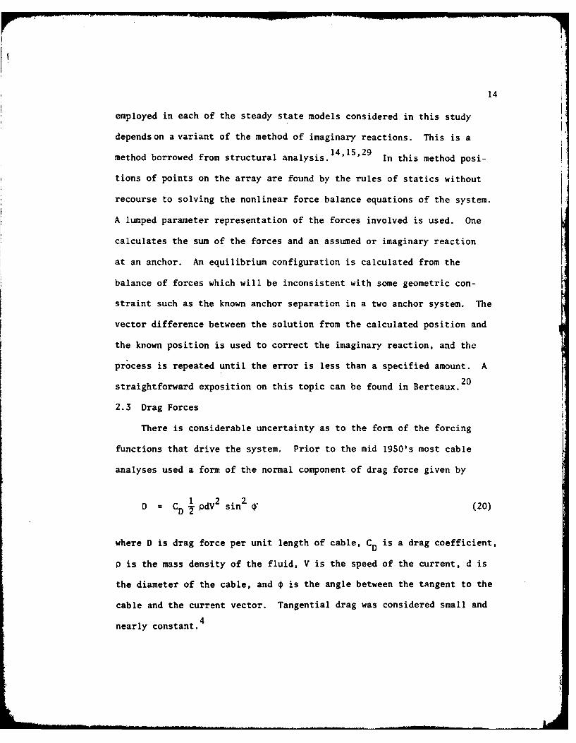
2.3 Drag ForcesI.
There is considerable uncertainty as to the form of the forcing
functions that drive the system. Prior to the mid 1950's most cable
analyses used a form of the normal component of drag force given by
D = CD 7 PdV2 sin c (20)
where D is drag force per unit length of cable, CD is a drag coefficient,
p is the mass density of the fluid, V is the speed of the current, d is
the diameter of the cable, and 0 is the angle between the tangent to the
cable and the current vector. Tangential drag was considered small and
nearly constant.4
isi
15
More recently, however, this simple drag model has been found in-
adequate, particularly with respect to tangential drag. Even though the
values of the tangential drag force are two orders of magnitude smaller
than the normal drag force, in many cable problems, it can be important. 1030
A commonly used force model was formulated by Eames. The normal com-
ponent of force per unit length of cable is given by,
pdC D 2pdCD2 V2 {(l-u) sin 01sin 01 + p sin 0} (21)Fn - 2
The tangential component of force per unit length of cable is given by
F PdC D V 2 Iv cos 0 + v cos 01sin fl} (22)
F n is normal component of force,
F t is tangential component of force,
p is density of fluid,
CD is drag coefficient,
0 is angle between cable tangent and flow direction,
d is diameter of cable,
.is friction coefficientboth range from 0.025 to 0.05.
v is form drag coefficient3
Wilson10 summarized a large number of drag coefficient measurements
as a function of Reynolds number. From his data we get the commonly used
values of 0.9 to 1.2 for smooth cables and 1.4 for rough cables in the
Reynolds number range commonly found in the sea. There is considerable
j!

16
scatter in the data, however, and any particular cable is likely to vary
from the norm. For example, Kretschmer, Edgerton, and Albertson3 1 per-
formed wind tunnel tests on a jacketed cable 1.8 cm (0.705 in.) in
diameter and obtained drag coefficient values of 1.55 for the Reynolds
number range commonly experienced in the ocean. This is somewhat higher
than the results for smooth rigid cylinders.
The Reynolds number of the flow is given by
R = V pVd (23)e V
where
R is Reynolds numbere
v is kinematic viscosity
U is dynamic viscosity
d is diameter of the cable
V is velocity of flow
p is seawater density,
Typical values for the parameters applicable to the experimental data
that will be presented later are: V at 4*C = 0.016 gm/cm sec, 3 2 d = 4 cm,
3V = 2 to 10 cm/sec, and p = 1.025 gm/cm . Substituting these values in
equation (23) gives a Reynolds number range of 0.5 x 10³ < Re < 2.6 x 10
The drag force equation used in the Griffin model and the Patton
model was that given by equation (20) with the value of CD calculated as
follows for the normal component of drag force:
F[R- 200C D 1.2 e 8000 J 200 < Re < 25,000 (24)Df 500(4

17
FR e-2500]cD 0. I e I S0<RC =0.9 e 43,000 2500 R < 15,000 (25)
CD = 1.2 15,000 < Re < 200,000 (26)
The tangential component of drag was calculated from
FT 1 C d V2 Cosflcospl , (27)FT = DT o
The expression for the tangential drag coefficient used is based
on a study by Wilcox:3 3
CDT = 0.8 (RT) -0.77 < RT < 102 (28)
DTeT -. 2 1 R 1= 0.2226
CDT = 0.0635 (ReT) 10 < ReT < 10 (29)
where ReT is the Reynolds number calculated for the tangential component
of the flow velocity.
2.4 Strum Amplified Drag Coefficient
There is a further complication to the drag coefficient issue. It
is well known that cables in a moving fluid will experience flow induced
21strumming vibrations. If the strumming frequency approaches the
natural frequency of the cable then resonance can occur. The result
of this is a greatly increased drag. This idea is used to explain why
the observed cable displacements are often much larger than the models
predict. Skop and Rosenthal34 have introduced a strum amplified drag
coefficient in the DESADE static model to bring the calculated cable
L,

18
displacements into better agreement with observations. They give a
formula for the strum amplified drag coefficient, CDA' for horizontal
cables:
CDA = 1.69 Rl.09
n= 1 +~ 4.61)2.16 (30)
CDO ( +46
where CDO is the drag coefficient for a nonstrumming cylinder and Rn is
the Reynolds number for the flow based on the component of current nor-
mal to the cable axis;
Vd
R = n (31)n V
where Vn is the normal component of flow and v is the kinematic viscosity
of the fluid,
The strumming frequency is determined by
S V
= nd (32)
d[
where S is the Strouhal number, V is the velocity component of then n
current normal to the cable, and d is the cable diameter. For Reynolds
numbers between 103 and 104 the Strouhal number is nearly constant
"0.21. 5
The data base on which to decide a priori whether a cable will strum
36or not is very skimpy. Kennedy and Vandiver summarize the results of
four experiments which attempted to measure strumming effects. All of

I. 19
the experiments suffer from one defect or another, but they were able
to draw the following conclusions;
1. Excitation process seems to be a narrowband random process
centered around the Strouhal frequency.
2. Many modes of cable oscillation are excited - as many as 50
or 100.
3. Resonant lock-on of cable natural frequency with vortex
shedding frequency was observed only rarely.
4. There appears to be a self limiting mechanism for the amplitude
response which does not seem to be affected by cable length,
virtual mass, damping, number of modes excited, or flow speed.
S. The amplitude of the nonresonant response was about one quarter
of a cable diameter,
The literature on vortex induced oscillations is large and there
are two excellent review articles by King5 and Sarpkaya. There is a
great deal of controversy in the field and different arguments can be
brought to bear to explain the results quoted above. Aside from the
work of Skop and Rosenthal 34(it will be shown later that equation (30)
leads to unrealistically high values of the drag coefficient when
applied to the experimental data) there is little help for the modeler
who is interested in modeling the large scale behavior of cable systems.
The simplest way to account for strumming phenomena is to adjust
the drag coefficient, or equivalently, increase the effective cable
diameter in the drag force equations. Dale and McCandless suggest a
drag coefficient increase of 38 percent based on experimental data with
short cables in a tow tank. 38Conclusion 5 in the preceding list taken

V n i e 36 20
from Kennedy and Vadvr suggests that an increase of effective cable
diameter of 25 percent would be appropriate. In the results that follow
several drag coefficients will be employed as will an increased effective
cable diameter.
2.5 Added Mass
If a cable immersed in a fluid is accelerated, the force required
is larger than the force to more just the cable. This is because a part
of the fluid must also be moved around the cable.. An expression for the
force per unit length of cable is
F =(m +m) dv (33)a a dt
where m a is the added mass. The quantity (m + m a) is referred to as the
virtual mass. The added mass per unit length of cable can be calculated
from
ma C 7 d2 (34)
where C Mis the added mass coefficient, p is the density of the fluid,
and d is the cable diameter. C mcan be calculated from potential theory
for nonrotating flow of ideal fluids. 39The value of C m calculated for
a sphere is 0.5 and for a cylinder is 1.0. Patton 40 ,alculated added
mass coefficients for a variety of shapes.
In practical problems, however, we are likely to violate the assump-
tions under which C m is calculated. For these problems the added mass
should be measured experimentally. Ramberg and Griffin 41provide a
method for measurement of virtual mass by measuring the ratio of

21
resonant frequency in air to resonant frequency in water. Virtual mass
in water is then calculated from
Nwater = f) Mair
where fa is resonant frequency in air and fw is resonant frequency in
water. Pattison, Rispin, and Tsai4 2 provide a collection of measured
values of virtual mass.
There is some evidence that there is a frequency dependence to the
added mass. Patton,9 citing experimental results of Miller4 3 and Miller44
and Hagist, used the following expression:
m = 1.0 - 1.62 X 10⁻⁶ _ d2 p (36)
where w is the frequency, d is the cable diameter, and v is the kinematic
viscosity. It is seen that the quantity outside the parentheses is just
the added mass of a circular cylinder of unit length. There is also
45evidence in experimental results reported by Ramberg and Griffin that
there is no frequency dependence to added mass. The issue is presently
unresolved. This study will use the Patton expression. The questions
that need to be addressed in order to resolve this issue are discussed
by Sarpkaya.3 7

3. PESCRIPTION OF EXPERIMENT
3.1 OMAT Background
The data reported in this study were obtained as a subset of meas-
urements from a larger experiment. The overall experiment, the Ocean
Measurements and Array Technology (OMAT) program, was directed toward
system-oriented measurements relative to large aperture acoustic systems.
Thus the primary objective of the program was to provide a highly flex-
ible, large aperture acoustic array that could be deployed, recovered,
and reconfigured together with associated processing and real-time analy-
sis equipment so that a variety of array/system concepts could be tested
using essentially the same hardware, The system was deployed three times
in a series of experiments at sea that were conducted during the sumers
of 1977, 1978, and 1979. The portion of the overall experiment that will
be discussed here is the study of the motion of the array cable in the
ocean currents.
The general configuration of the experiment is shown in figure 2.
The water depth was 5.5 km. The horizontal span was 6 km long and
buoyed to a nominal height above the sea floor of 2.7 km. Within a few
hours of the beginning of the experiment, an electrical failure developed
in approximately the last one third of the cable so that the only use-
able data were from the eight position sensors closest to the umbilical.
The physical description of the cable system is given in table 2.
The measurement site was in the southern Sohm abyssal plain region
near 32° N 570 W. The site was chosen initially because it was believed
to be quite flat bathymetrically and in an oceanographically quiet
22

23
MAYE
UMBILCAL 5 KM RANSPONOERS/CURRENT ME TERSCABLE
COMND OS ON RECOVERY
TAG LINE
Figure 2. Experiment Configuration

24
portion of the North Atlantic basin. A bathymetric survey was conducted
in the area and a number of small hills were seen to poke out above the
generally flat surroundings. Figure 3 shows the results of the site
survey and the locations of the anchors and the current meter arrays.
Table 2. Physical Characteristics of the OMAT Cable System
Cable Buoyancy inComponent Diameter Length Sea Water Spring Constant
Umbilical 4.953 cm 9146 m -2,115 N/m 1.0196 X 10⁷ N/m
Active S.874 cm 3088 m 4.377 N/m 2.5106 X 10⁶ N/mRiser
Horizontal 5.239 cm 5985 m 0.3647 N/m 2.5106 X 10⁶ N/mSpan
Inactive 8.6 cm 3088 m 0.4377 N/m 2.3342 X 10⁶ N/mRiser
Tag Line 4,128 cm 9146 m 0.0 N/m S.712S X 106 N/m
A profile measurement was made of temperature, salinity, and sound
speed as a function of depth. Density was calculated from the profile
measurements and from these data the Brunt-Viis~li frequency was calculated.
The profiles of salinity, temperature, sound speed and Brunt-Viisili fre-
quency are given in figure 4.
3.2 Cable Shape Measurements
The shape of the cable was measured acoustically. The cable shape
measurement system consisted of a pinger on the cable, 13 position sen-
sors spaced along the cable, and three transponders located broadside to
the cable. Figure 5 shows the arrangement of the components of the cable
shape measurement system.

25
I6w 40 .0 2o w iw
40
U-
20'w
10! -id
. .... I I .. .. . . . . i .
igW u 40 20' 20o th Si'W
Figure 3. Bathyntetry off the Site
,I

26
0
o 0
TN+- I
>0 ww
zr w
0 0 El
LEl
0 0 In
0 0 *Jton
0 -: :6

27
-YV
FINAL OMAT ARRAYCONFIGURATION
6 (TO SCALE)
5-TRANSPONDER
FIELD4 T1 T2 3
POSITIONSENSORS
2 -x 2 .7 9 0 M 1 I G
BOTTOM
I 2 3 4 5 6 7 8 9 10X(KM)
Figure 5. Configuration of Acoustic Cable Shape Measurement System

28
Table 3 lists the locations of the position sensors relative to the
end of the cable.
Table 3. Location of Position Sensors on the Cable
Sensor Distance fromNumber End (m) Remarks
1 24.06
2 1082.75
3 1428.25
4 1913.75
S 2035,75
6 2593.25
7 2930.25
8 30S2.75
9 3389.75
10 3943.25
11 4069.25
12 4900.25
13 5958.36 colocated with command pinger,tensiometer and pressuresensor.
The method of cable shape measurement was developed by Callahan.46
Since his report is unpublished, the features of the technique required
to understand the data are summarized here.
The measurement process was initiated on board ship by sending a
signal that caused the pinger on the cable to transmit an 11 kHz pulse.
This pulse was received at each of three transponders located off to the

29
side of the cable. The transponders then responded by sending a 9.5,
10.0, or 10.5 kliz pulse, depending on whether the responding transponder
was T1V T or T A signal sequence was then received at each of the
position sensors on the cable, All of the received signals were sent
via an umbilical cable to a ship nearby where they were stored in a time
of arrival matrix for subsequent processing. All of the times stored
were relative to the initiating signal sent from the ship.
Acoustic travel time was then converted to slant range using sound
speed data measured just prior to the start of the experiment. The sound
velocity profile was approximated as piecewise linear. The velocity in
layer n is given by
v(z) = a + bn (z - z n) z < z < z (37)(37)n n) n n n+l (7
The time for a vertically propagating ray to travel from depth d1 to d2
is
dz
T(d,d 2) f z (38)
d1
The average sound speed between depth d1 and d2 then is
Id1 - d2 1vd(dl,d 2) T(dlad 2) (39)
for direct path transmission and
Id1 + d21vs(d1 ,d2) = T(O,d1 ) + T(d2 0) (40)

30
for surface reflected paths, Slant range is then calculated by multiply-
ing the average sound speed for the appropriate path by the observed
acoustic tra-el time. This development assumes straight line ray paths;
the error caused by this assumption will be discussed in section 4.2.
The pinger depth was determined for each ping by measuring the round trip
travel time for the surface reflected ray and converting to depth. The
depth of each position sensor R was then calculated for each ping from
the known pinger depth T, the direct path length D, and the bounce path
length S, according to the relation
2 _2R = (S2 D )/4T (41)
The geometry for depth determination is shown in figure 6. Equation (41)
is derived using figure 6 by application of the law of cosines:
D2 = a2 + b - 2ab cos . (42)
Then, drawing the bisector of 6 gives
COS R (43)
os2 a
The half angle formula gives
1 + cos 0 R (44)2 a
Solve for cos 0 and substitute in equation (42). From the properties
of similar triangles

31
SURFACE
T
POSITION \
SENSOR
~~DIRECT \
S=o~b
PINGER
Figure 6. Depth Determination Geometry
32
b Ta (
Making this final substitution and rearranging gives equation (41).
With the depths of all the elements established, it was then pos-
sible to project the geometry onto the horizontal plane and calculate
the remaining coordinates of each of the sensors. Subsequent calculation
would have been straightforward if the transponder positions were known
exactly; however, a survey of the transponders conducted from a surface
ship shortly after they were installed was not sufficiently accurate.
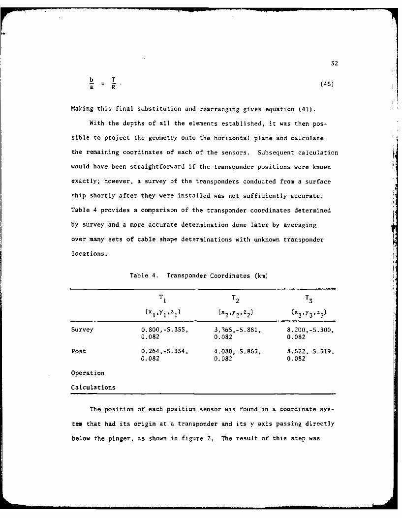
Table 4 provides a comparison of the transponder coordinates determined
by survey and a more accurate determination done later by averaging
over many sets of cable shape determinations with unknown transponder
locations.
Table 4. Transponder Coordinates (km)
T T T1 2 3
(xlYlz 1) (x2,y 2 ,z2) (x3 ,y3 ,z3)
Survey 0.800,-5.355, 3,365,-5.881, 8.200,-5.300,0.082 0.082 0.082
Post 0,264,-5.354, 4.080,-5.863, 8.522,-S.319,
0.082 0.082 0.082
Operation
Calculations
The position of each position sensor was found in a coordinate sys-
tem that had its origin at a transponder and its y axis passing directly
below the pinger, as shown in figure 7, The result of this step was

33
ddc
PIN GER
- -dT(PyT~T
TRANSPONDER(0 0, drT)
Figure 7. Geometry for Determination of Position SensorLocation in a Transponder Coordinate System

34
location of all the position sensors in each of three coordinate systems
which differ in both origin and orientation, as can be seen in figure 8.
The coordinate systems were then rotated and translated by an amount
such that the resulting position sensor locations most nearly agreed
in a least square error sense,
At this point, what we have is a self-consistent estimate of the
position sensor locations, but what we really want is to determine the
position sensor locations in a system relative to the two array cable
anchors. In order to do this a further fit of the transponder positions
was made to the positions obtained from the survey, as this is the only
connection between the transponder positions and the array cable anchor
Then, one last rotation and translation is performed to get the
final position in the anchor coordinate system,
3.3 Current Meter Measurements
Ocean current data were obtained from two vertical current meter
arrays. The two c-rays were separated horizontally by 4 km. The
location of the measurements was the southern Sohm Abyssal Plain. The
array positions relative to the local bathymetry are shown in figure 3.
The two arrays were identical, Each array consisted of three Aanderaa
RCM 5 current meters. The configuration of the current meter arrays is
shown in figure 9, The current meters were epoxy-coated to avoid the
compass problem that the older nickel-.coated Aanderaa instruments experi-
enced when subjected to high pressure. 47The instrument heights off the
bottom were 646 m, 921 m, and 1S30 m. The arrays were designated EA 1
and EA 2 and individual meters on an array were indicated by the suffix

35
NEARANCHOR + X
COMMAND
RIGHT PINGEREND PNEETRANSPONDER 3
COOROINATESYSTEM
0TRANSPONDER 2COORDINATESYSTEM
LEFT +Y
ANCHOR ENDCOORDINATESYSTEM
TRANSPONDER ICOORDINATE
+Y ySYSTEM
* ARRAY MEASURED TRANSPONDER POSITIONS
LYNCH MEASURED TRANSPONDER POSITIONS
Figure 8. Transponder Coordinate System and theAnchor Coordinate System

36
HEIGHT OFF BOTTOM MAJOR COMPONENTS
1585 M 43.2 CM GLASS BALLS-z FOR BUOYANCY
43.2 CM GLASS BALL
1530 M AANDERAA RCM- 5-- . CURRENT METER
143.2 CM GLASS BALL
921 M AANDERAA RCM-5
43.2CM GLASS BALL
646 M AANDERAA RCM - 5
TRANSPONDERS FOR82 M RELEASE SYSTEM
AND ACTIVE ARRAY SHAPEMEASUREMENTS
ANCHOR
/// BOTTOM ///////////,--/-.-z/-/z-,r
Figure 9. Current Meter Array Configurations

37
TOP, MID, or BOT; so, for example, the meter at a height off the bottom
of 1530 m on EA I would be designated EAITOP. The sample rate was 5 min.
In addition to current speed and direction, each current meter also
measured temperature and pressure. The current meter sensor character-
istics provided by the manufacturer are given in table 5.
Table S. Sensor Characteristics of Aanderaa Current Meter
Range Resolution Accuracy
Speed 0 to 125 cm/sec 0,1 cm/sec 0.5 cm/sec
Direction 0 to 3600 0,03o 5"
Temperature -2 to 200C 0,02-C 0.10C
Pressure 0 to 562 kg/cm2 0.549 kg/cm 2 5.62 kg/cm 2

4. RESULTS
4.1 Measured Cable Shape
A scatter diagram of the x/y coordinates of the position sensors
for the entire experiment is shown in figure 10. Inspection of the
figure shows that the scatter is not symmetrical about sumed anchor
baseline. This is probably due to an error during the survey of the
anchor locations. Other acoustic sensors on the cable were used to
determine the bearing to a distant sound source. That data indicated
an error in the anchor baseline of a degree or two. In order to correct
for this, a least squares regression line was calculated for the data.
The slope of the regression line was 1.50. The shape data has been
corrected by this amount.
From figure 10 one can see that the maximum excursion of the array
in the y direction was ±100 m, while the maximum excursion in the x dir-
ection was ±25 m.
In order to obtain an intuitive idea of the processes taking place,
an average transverse component of the motion of the horizontal span was
formed. The average was plotted as a time series in figure II. The
average was formed from the y component of position of the four position
sensors near the middle of the span. The data are not taken at uniformly
spaced times, so to get a curve for comparison purposes a spline curve
was fit to the data.4 8 The interesting feature of this plot is that the
oscillations were about ±100 m with a periodicity of about 12 hr. The
excursions were larger toward the end of the time series corresponding
to the time that the currents swung around more nearly broadside to the
38

39
ARRAY ELEMENT POSITION PLOTS (PLAN VIEW)
0.3
0.2-0l -w PV 13
z ASSUMED ANCHOR0BASELINE
PV 100 -0.1 PV# 1
0. PV5 PV6 PV8 PV9 PV 12
-0.2
-0.34.0 4.5 5.0 5.5 6.0 6.5 7.0 75 8.0 8.5
X COORDINATE
Figure 10. Scatter Diagram of Position Sensors

40
.2.
:.0
w
-j
204 205 2'06 207 208 209 '210JULIAN DATE
Figure 11. Time Series of Average Position Of Cable

41
cable. Times on the plots are given in Julian date ( a table for con-
version of Julian data to calender date is given in appendix A).
Similar averages were formed for the x and z components. These
49data were further analyzed using a maximum entropy technique. This
technique is particularly applicable to spectral estimation from short
records. It avoids many of the windowing problems that occur when deal-
ing with a finite data set. It is also useful for dealing with records
that have missing or bad points. What the technique does is to create
an autocorrelation function which is extended beyond the normal limit
of lag values using a predictive filter. The power spectrum is then cal-
culated from the autocorrelation with much reduced influence of end
effects caused by the short initialtime series. The spectra that result
from this analysis are shown in figure 12. The peak in the x and y com-
ponent occurs in the bin centered around 12.2 hr period. There is only
a small peak in the z component motion.
There were three pressure sensors included along the cable. The
sensor designated Dl was colocated with the command pinger. Sensors D2
and D3 were near the middle of the cable. The sensors D2 and D3 were
observed to drift considerably during pressure testing. The problem was
detected too late to change the sensors before the system was deployed.
They cannot be considered reliable. Sensor Dl, however, did not exhibit
the same drift characteristics. Its output is considered reliable.
The output from each pressure sensor was converted to depth and then
plotted as height above the sea floor. The resulting plot is shown in
figure 13,

42
N0
FRACTIONAL POWERN VERSUS
0FREQUENCY BIN NUMBER
BIN NO. PERIOD (HO URS)1 73-30
_ 2 36 65x3 24,43
4 18.325 14.66
0 6 12.21x7 10.47
8 9.169 8.14
0 10 7.33Zx II6.66
N12 6,10
WNC
0oxxMOTIONS
0y MOTIONS0 z MOTIONSx
0
xNY
1 2 3 4 5 6 7 8 9 10 11 12 13 14 15 16
Figure 12. Spectra of X, Y, Component of Average CableDisplacement

43
- JULIAN DATE
o 0N NY N N Nl Nu N N l
3500 D
D3
U3000
050
0
wx- 2000
050
Fiue1. Dph0esrOtu

44
The height measured by sensor Dl was in agreement with that cal-
culated for the command pinger to within the resolution of the depth
measurement. The resolUtion was 30 m.
There is a large depth excursion beginning on Julian day 211.
During this tine the umbilical cable becamne fouled in the riser. None
of the data from this period was used in this analysis.
The cable shape observations chosen for analysis are shown in
figures 14 to 19. The observations are broken dow-n into two periods.
The first period, designated run 1, covers the period 07101 to 1311 on
day 20S. During this time the cable moved from a southerly position to
a northerly position. The second period, designated rum 2, covers the
time from 1343 to 1833 of day 205. During this time the cable moved
from a northerly position to a southerly position.
4.2 Sources of Error in Cable Shape Measurement
The position sensors did not always receive signals from all possi-
ble paths and, in addition, under conditions of low -ignal-to-noise ratio,
some sensors did not immediately make a detection. Missing pings were
detected by sorting arrivals by ray paths, but the second error, the
delayed detection, was more subtle and data flawed by this error was
sometimes included for analysis. In order to find this flawed data, a
check of the calculated straight lime distance between adjacent sensors
was performed. If the distance between the sensors calculated from the
data was greater than the known distance along the stretched cable, then
one of the two points was bad. The bad one was determined by performing
a similar check using combinations of adjacent sensors.

45
T00001
0008-
00090mI N -n N~.J, n
- 4-
o
x
0 0
00 C
Ca 0 tm
rj

46
0008
0 0
0001F
000g-
oo
Lnn
I " I I 00 I
m 4)
( J Ox
.. . . . . I l . . . . . . . . . .. .. .. ... . ... . .

47
1311
1 295 0
1134 0Cu
0 $40 LCoL
o,0.D
ba
-4
(W) W~wup..ooz Z
0!

48
0000!
0008
co CD
1 0
0001F
r-~o 'ij, i~- pm
L 06

49
00001
0008
0009
- CC
L 0v
oooo
100
L4)r1-.
(W)0-0 vp co4)

50
oso
1343 .
1652 41fl24 B o0
0 .
155 r1 725
ls
oo
(H)0-40C)0 JCu-
Ci
(H) e o,-t p.Cooo
i,,. L ,
r r I l . .. . . .. . ... II l I .. . ... .. .... . .. .. .. . ... . .. ... . .. . . . . . ' r I
51
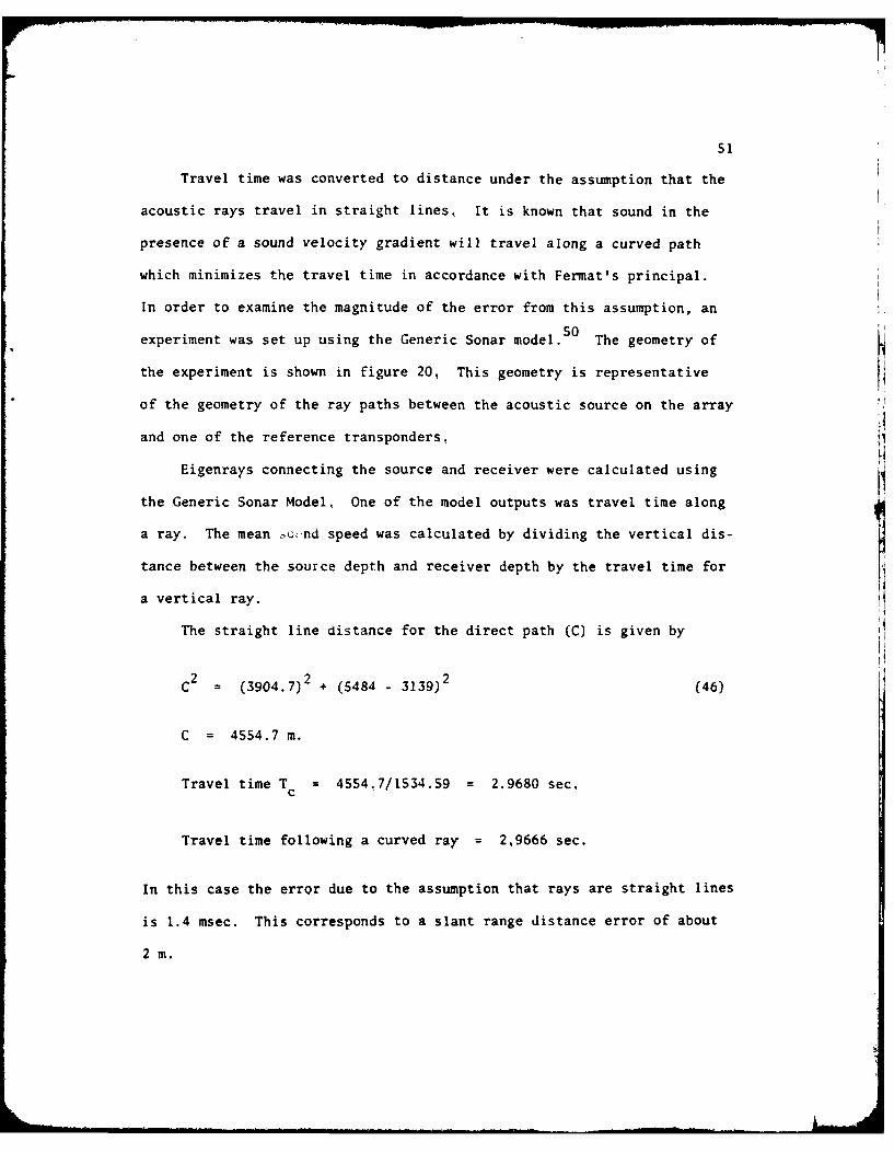
Travel time was converted to distance under the assumption that the
acoustic rays travel in straight lines, It is known that sound in the
presence of a sound velocity gradient will travel along a curved path
which minimizes the travel time in accordance with Fermat's principal.
In order to examine the magnitude of the error from this assumption, an
experiment was set up using the Generic Sonar model. The geometry of
the experiment is shown in figure 20, This geometry is representative
of the geometry of the ray paths between the acoustic source on the array
and one of the reference transponders.
Eigenrays connecting the source and receiver were calculated using
the Generic Sonar Model. One of the model outputs was travel time along
a ray. The mean ,tnd speed was calculated by dividing the vertical dis-
tance between the source depth and receiver depth by the travel time for
a vertical ray.
The straight line distance for the direct path (C) is given by
C2 (3904.7)2 + (5484 - 3139)2 (46)
C = 4554.7 m.
Travel time T = 4554.7/1534.59 = 2.9680 sec,c
Travel time following a curved ray = 2,9666 sec.
In this case the error due to the assumption that rays are straight lines
is 1.4 msec. This corresponds to a slant range distance error of about
2 m.

52
a-3904.7m-.a- xSEA SURFACE
C=1515.65 r/
b a
SOURCE 3139
5484m R C E 11 EE RRCZ1534.59 r/s
5484r RECIVERBOTTOM
5566 m
Figure 20. Geometry Of Model Experiment to Test the Effects of Ray Curv-ture on Acoustic Travel Time

53
The straight line distance for the surface reflected path (a + b) is
determined using the properties of similar triangles to obtain simultan-
eous equations:
390 4 - x x (47)3139 5484
3139 5484b (48)a b
2 2 2(5484) +x = b (49)
Solving this set of equations yields;
x = 2482.8 m
b = 6020.0 m
a = 3445.8 m
Travel time T = 9465.8/151S.65 = 6.2454 sec.
(a~b)
Travel time following a curved ray = 6.2451 sec.
In this case the error due to the assumption that the ray travels in a
straight line is 0.3 msec. This corresponds to a slant range distance
error of about 0.5 m. The smallness of the error in this case is prob-
ably fortuitous since the accuracy of the eigenray calculation is about
1 msec.
A further source of error in the cable shape measurement comes from
the fact that the bottom mounted reference transponders are actually
buoyed up from the sea floor to a height of 83 m. The mooring is then
subject to action by ocean currents. The result of a mooring deflection

$4
study is shown in figure 21. Under the conditions experienced during
the experiment the calculated transponder positions would not be expected
to vary by more than 1 or 2 m,
A possible source of error comes from the fact that a single sound
speed profile was used for conversion of travel time to distance. Sur-
face heating, mixing processes, water mass advection or internal waves
could alter the sound speed profile. A check on errors from this source
was performed by adding the round trip travel time from the pinger to
the surface to the round trip travel time from the pinger to the bottom.
Since the distance from the surface to the bottom was fixed, any important
differences in mean sound speed would be reflected in the travel time.
The average travel time was determined on three different days and the
difference of the averages was tested for significance using student's
T test. There was no significant difference in the means at the 0.01
level. Consequently we can say that the changes in the sound speed pro-
file that may have occurred did not produce appreciable changes in the
average sound speed used in the conversion from travel time to distance.
4.3 Ocean Current Data
Time series plots of ocean current measurements are presented in
figures 22 and 23. The data were corrected for magnetic variation (180W)
and then resolved into components along axes oriented toward North and
East. The component data were then filtered with a lowpass Butterworth
filter (1 pole). The high frequency cutoff for this filter was I cycle/
hr. The data were then resampled at half hour intervals. In order to
obtain the data set presented in the figures, a further rotation was
made to a heading of 125"T, the nominal line of bearing of the line

55
SUBSURFACE FLOATCURRENT METER
1400
1200
5CM/SEC1000 10 CM/SEC
CURRENT METER
4 00
I.--0
U.U.0
o600
Z CURRENT METER
OMAT 1979 EA ARRAYSMOORING DEFLECTION
200
TRANSPON DER
10 20 30 40 50 60 70 80 90 100
DEFLECTION (M)
Figure 21. Transponder Array Deflection in Gcean CurrentsL

56PARALLEL COMPONENT
-------------- PERPENDICULAR COMPONENT
U,
1~ 4zz 20 A
0
z
w~
ua U EAIMOTCL
I- 4z
0A s
0 ,, .11, *' %0I
w %j
Figue 22 TimuSeies ofCrenaopnettera n
Paale o alefo EA IT

S7
PARALLEL CO;-4PONENT
----------------- PERPENDICULAR COMPONENT
z
aU0 -2 ,
z
~ 8 EA2MID
a.4
z0
z
w0r
F.- 4
z0
z
Figure 23. Time Series of Current Components Normal andParallel to Cable from EA 2

S8
connecting the two cable array anchors. Here a positive parallel corn-
ponent is toward 305 0T; a positive perpendicular component is toward
0 3S T.
This same data set is plotted on a progressive vector diagram in
figures 24 and 2S. At measurement site EA 1 the currents up to 26 July
(Julian day 2107) are generally in a direction of 1160T. The currents
then swing south for a day then to the southwest. This process begins
a day later on 27 July (day 205) for the middle current meter. At
measurement site EA 2, the currents are generally the same at all three
levels in a direction of 120*T. Then on 24 July (day 210) the currents
at the two deeper meters turn toward 140 0T while the top meter continues
to show currents toward 1200. On 26 July currents at the two deeper
meters swing back toward 100*T. Not until 29 July do the two deeper
meters indicate a current swing to the south, three days later than the
similar event at station EA 1 (remember that the horizontal separation
of the two arrays is only about 4 kmn).
It is interesting to note that these data are inconsistent with the
general circulation model of the North Atlantic of Worthington. 5 1
Worthington's model predicts westerly currents at a depth of 4000 m at
the measurement location. Owens and Hogg 5 2 reported similar anomalies
in current measurements made near a bathymetric "bump" of similar dimen-
sion to the "bumps" in the vicinity of these current measurements.
Power spectra of the current magnitude were calculated for each
meter. The spectra are shown in figures 26 and 27. All spectra have a
peak at about 0.08 cycle/hr, which corresponds to a period of 12.5 hr.

59
2"fl2 5- 5 2632 - 35.6 'N 56 25 - 27
901 " JERTr 556-" 26
L 23 jULY 99Z1E 4 Q O 28C''5 :SGTjCM~' 27 ,7
-5 C' : 75 -OSOM NO 5Y5OL
Q- -8 1 o 5 , 6 's " 9o . ' 2 8 /
255' '9'~ c'os 29
SM83OLS qt 2000O2"
23 - 30 J.L I; -i5 2
30
-2c 30/
-2
- 3 I 1 f t I t I15 -10 -5 0 5 10 15 20 25
EAST OISTNCE. KM
Figure 24. Progressive Vector Diagram for Current Meters on EA 1
I I IA

60
52
- 32 - 342'N 56 - 2 \
gotta" 0-1-~ 5567M
Z 1" 776 4010" NO S7"SOL 25 26-E 4157 4680M Sol 2
In1156 1980" z9055
5r'eaLS AT D000CM! 26 2723 -30 JULY
~ -1 30z
30
-25
-i5 -10 -5 0 5 10 15 20 25EPST OISTANCE. KM
Figure 25. Progressive Vector Diagram for Current Meters on EA 2

61
20.0 1il I~l6
10.0 ESO
-10.
0 2.
- -0.0 -
S-20.0-
-30.0--- 0.0--70.
-80.0-
0.00 0.01 0.10 5.00 10.00
30.0-20.0-
1- 0.0 -0. -
U-10.0 - -
- 20.0
-- 30.0 -
- 40.0-
-70.00.00 0.01 0.10 1.00 50.00
30.
210.0 -
--0.0 ------ ~----
-70.020.00 .505 .050
FR30.0YCP
Fiue264ure0.0itd petaFrmE

62
20.0 1 T E AMIOP20.0 i:t
S0.0
-0.0 Vo 20.0
-30.0 -
*~-40.0-50.0
-60.0 I
-70. 00.00 0.01 0.10 1.00 10.00
30.0 E2I
20.0 -I -10.0
-0.0
--50.0
-20.0 -
- 70.0
0.00 0.01 0.10 1.00 10.00
30.0
(L 10.0
S0.0
T -10.0
-30.0
-40.0 -
-50.0
- 60.0
- 70.00.00 0.01 0.10 1.00 10.00
FREQUENCY, CPH
Figure 27. Current Magnitude Spectra from EA 2

63
At the latitude of the measurements the inertial period is 22.3 hr. The
period of the M2 constituent of the tide is 12.42 hr.3 2
4.4 Static Mode~s
Two static models were investigated. The DESADE model was of the
imaginary reaction type, the GRIFFIN model solved the steady state
differential equations and used the imaginary reactions for determining
the boundary conditions.
The most widely used static model is the DESADE model developed at
the Naval Research Laboratory. 14 ,15 The model considers only the normal
component of the drag force and in its original version permitted ocean
current variations only as a function of depth. The most significant
modification of the program by other users is in the provision for
complicated current fields which vary in the horizontal as well as inthe ertcal53'54
the vertical. 5 4 The principal limitations of the model from the
point of view of the present study are that the cable structure cannot
consist of more than 22 segments and the neglect of tangential drag.
Provision has been made to introduce a strum amplified drag coefficient
34which is a function of Reynolds number. Plane and side views of the
DESADE output for various current speeds broadside to the cable are
shown in figures 28 and 29. Listings of the data are provided in
appendix B. Additional runs were made for several values of the drag
coefficient. The maximum deflections of the cable by currents of 2.5
cm/sec are shown in table 6 for various values of the drag coefficient.
The effect of changing the drag coefficient can be dramatic, as seen
(for instance) in figure 30. This is a plot for the strum amplified
drag coefficient calculated according to Skop and Rosenthal.3 4

64
200015 CM/SEC r
1 500
z
1000 1 M-
0
500
1000 2000 3000 4000 5000 6000 7000 8000 9000 10000X COORDINATE M)
Figure 28. Plan View of Cable Configuration Calculated by StaticModel for Currents of 2.5, 5, 7.5, 10 cm/sec.

65
2500-
200012.5 CM/SE 7.5 CM/SEC2.5 CM/SEC
15 CM/SEC 10 CM/SEC
zt 150000
N
1000
1000 2000 3000 4000 5000 6000 7000 8000 9000 10000X COORDINATE (M)
Figure 29. Side View of Cable Configuration Calculated by StaticModel for Currents of 2.5, 5, 7.5, 10 cm/sec.

66
2000 10 CM/SEC
2100
0
0 100 20 3000 4000 5000 6000 7000 8000 9000' 10000X COORDINATE (M)
Figure 30. Static Model Output Including Strum Amplified DragCoefficient

67
Table 6. Maximum Displacement c Cable forBroadside Current of 2.5 cm/sec as Function
of Drag Coefficient
C D Maximum Displacement(m)
1.2 63
1.3 68
1.55 81
Strum Amplified 157
CD
The GRIFFIN static model used is one developed at the Naval Under-
water Systems Center. 55 2 8 This method computes the boundary conditions
by the method of imaginary reactions. The steady state differential
equations are then integrated using a fourth-order Runge-Kutta method.
This model features a Reynolds number dependent drag coefficient and
includes the effects of tangential drag. The output of this model for
several values of current is given in appendix B for comparison with
other results.
A time series of static model outputs corresponding to the times
of cable shape measurement in run 1 is given in figure 31. This plot
was generated by putting the observed currents at each time into the
GRIFFIN model and calculating the equilibrium shape of the cable. If
the cable was always close to an equilibrium condition, then this time
series would closely resemble the observed cable shapes during run 1
shown in figure 14. There are two things to note here. The first is
that all of the model displacements are smaller than the observed

68
000701
080
00
CL
0
0) 9CL
00
4)00.
0 -
0 .0
0 C
Iwocm-

69
displacements. This could be corrected by using a larger drag coeffi-
cient; however, the drag coefficient which would bring the model into
agreement with observations at 0700 would not be the same as the drag
coefficient required to accomplish the same thing at 1300. The second
thing to note is that the cable observations are not in static equili-
brium with the currents. The currents from 1000 to 1300 are very small
and yet the cable continues to move to the extended position observed
at 1311. This points up the importance of the dynamics in this problem.
4.S Dynamic Model
The dynamic model used is one originally developed by Patton 9 and
subsequently modified by Griffin. 56 It is a lumped mass model where all
of the essential dynamics can be considered to be taking place at a few
positions on the cable system. These positions are connected by hypo-
thetical massless springs and damping elements., The model treats tan-
gential and normal drag, elastic properties of the material, added mass,
and damping in three dimensions.
The cable system is modeled by nine lumped mass elements as shown
in figure 32. The dynamic cable equations are integrated using a fourth-
order Runge-Kutta method with a time step of 0.1 sec. The effects of
strumming were introduced by increasing the effective cable diameter by
25 percent, This was done based on the finding of Kennedy and Vandiver36
that the strumming amplitudes experience a self-limiting amplitude re-
sponse of about 25 percent of the cable diameter.,
The dynamic response of the cable system was studied using the
dynamic model. The cable was initially assumed to be at equilibrium
with no current. At time t = 0 a step function change of current of

70
z
LUMPED MASS ELEMENTS INDICATED BY6 ROMAN NUMERAL.
5
4
NI 3n 2
2
Y I 2 3 4 5 6 7 1 0 x
X(KM)
Figure 32. Schematic of Lumped Mass System

71
15 cm/sec broadside to the array was introduced. The computed time
history of the y component of displacement for lumped mass points IV
and VI are shown in figures 33 and 34. The time history curves have
the appearance of the curve of a charging condenser. The equation
which describes a charging condenser is
-rtY Ct + (Y - a) e (50)
An equation of this form was fit to the data using a technique given by
57 -jHoward, Griffin and Foye. The value for r was found to be 0.0111 X 10
-lsec The reciprocal of r is the time constant of the charging con-
denser. In this case the time constant of the cable system turns out
to be about 2.5 hr.
A time series of the calculated cable shape was created to corre-
spond to the sample times of the cable shape measurements.
The model was started from a position of equilibrium with no current.
The current input into the model was determined by fitting a Fourier
series to the hourly averaged data. Then the current at each time step
was calculated from the sum of the Fourier components. Figure 35 shows
the fitted data with the original time series for the parallel and per-
pendicular components of the currents from EAITOP. This is representa-
tive of the data from the other five current meters. Each of the six
current meters was considered to be acting on that portion of the struc-
ture that was closest. No attempt was made to compensate for the fact
that the current meters were 5 km away from the array. If changes in
currents at the current measurement arrays are due to a moving distur-
bance (waves, advection of turbulence, frontal passage etc.) then there

72
110-
100-
90-
80-
70-
~60-
Uj50-
40-
340
0
30
20
0 2,000 4,000 6,000 8,000 10,000 12,000 14,000 16,000 18,000
TIME (SEC)
Figure 33. Time History Plot of Displacement of Lumped NMass Point IV

73
100-
90-
80
70
~60
zLu 50-
_j40
0
30-
20-
00 2,000 4,000 6,000 8,000 10,000 12,000 14,000 16,000 18,000
TIME (SEC)
Figure 34. Time History Plot of Displacement of Lumped Mass Point VI

74
a. 0 J 4.
z0cr CLa
00LA. 00- -
0L-J
0o 4- 4w4
CLI
020
0111
U~~ m . .- c-N/ r-
0. c / - C .11c

75
would be a time difference between the time of an event at the measure-
ment site and the time of the event at the cable site. When the current
field is relatively homogeneous this will not be a problem. When the
currents are not the same over the area, such as was the case on
27 July for example, then the currents measured at the current measure-
ment site will not adequately describe events at the cable site.
The dynamic model was run for the currents that were measured on
days 205 and 206. A limited analysis period was a result of the fact
that the program requires 1 hr of computer time to calculate the array
response for 1 hr of real time on the PDP 11/70 computer.
The Fourier series expansion of the current meter data is given by
f(t) A + an cos+ b sin (51)
n=1 L B A/ Bk
where
XB
XB XA f(t) dt (52)
XA
XB / 2lnt\
a XB A f(t) cos X dt (53)
XB B2Bnt
XA f(t) sin dt (54)2 x -
..... B A ... . . .. .. ll Iln . .. ....-. .. . ". ... .

76
For our case
x - X = 24 hours X 3600 sec/hrB A
= 8.64 X 10 4sec
and t is the time in seconds.
Ile have data from EA-1 and EA-2 at three depths on each array. The cur-
rent speed was introduced in the model in the manner shown as follows.
Z EA-I EA-2
(VPLr)I (VPLT) 2(VPT), (VPT) 2
(VPLM) I VL)(VPM) I (VPM) 2
VPB)1(vPLB)2
g .x

77
Assume that
1. (VPB)1 and (VPLB)l act at element 1.
2. (VP M)I and (VPLM)l act at element 2.
3. (VPT)1 and (VPLT)L act at element 3.
4. (VP 1T) and (VPLT)I act at element 4.
5. (VPT)2 and (VPLT)2 act at element 5.
6. (VPT)2 and (VPLT)2 act at element 6,
7. (VPT 2 and (VPLT)2 act at element 7.
8. (VPB)2 and (VPLB)2 act at element 8.
The output of the dynamic model which corresponds to the cable shape
measurements of runs 1 and 2 is given in figures 36 and 37.
4.6 Sources of Error in Modeling Effort
The principal source of uncertainty in the modeling effort comes from
the fact that the current measurements were not colocated with the cable.
The current meter arrays were about 5 km from the array and were separ-
ated from each other by about 4 km. The currents at each array were
often different from one another and we must expect that currents at the
cable location would also be different. The bulk of the horizontal span
of the cable was 1 km above the highest current measurement. If there
were additional current variation with depth, the input to the model
could be seriously in error.
A further potential source of error comes from the fact that funda-
mental parameters of the array, drag coefficient and virtual mass, were

78
0000
8 -
I
V4 J
09 S4)oC
m 3 - - 3 V;; I -D* t-m * * L0
02
xU
0,,
4-
0
C-4-,
I,o
H
I--- -4- ~-- -- I
N N
~ A
I

79
0008
0009 r
4-,
U 31
0002
CYCajup000

80
not measured experimentally. The values of these parameters that were
used were estimated based on results for similar cables reported in the
literature., It is not known whether the cable was strumming or what the
magnitude of any strumming motions might have been. Consequently any
strumming effects introduced into the model are based on experience with
other cables, which may or may not be applicable to this specific model-
ing effort.
A check on the numerical performance of the models was performed by
introducing a test problem with a known solution. The simplest such prob-
lem is to consider the shape of a uniform, buoyant cable under conditions
of zero current. In this case the cable shape should be a catenary. The
equation of a catenary is
xZ = c cosh - (55)c
where c is the height of the directerix (here taken to be the x axis)
and is found from
S = c sinh x (56)c
for the case where the end points of the cable are at the same depth.
S is the distance along the cable from the maximum height to the end of
the cable and x is the coordinate of the end point. For the case where
the ends of the cable are not at the same height, C is determined from
2 h 7
(12= 2c sinh (57)T-c

81
where h is the horizontal separation of the end points, k is the vertical
separation of the end points, and I is the length of the cable. The
geometry of these two cases is shown in figure 38.
The result for the static model agreed with the analytical solution
to within a maximum difference of 0.4 m (table 7). The result for the
case of the dynamic model was that the maximum difference was 0.2 m
(table 8).

82
T
C
SP-
C
A Tk
Figure 38. Schematic of Catenary Used to Test Numerical Output of Models

83
Table 7. Comparison of Static Model Output to Catenary forUniform Cable, No Current
X Z (Model) Z (Catenary) Difference
0.0 0.0 0.0 -0.0
334.4 5lS.0 515.7 -0.1
694.9 1012.9 1013.0 -0.1
1084.5 1487.0 1487.1 -0.1
1506.6 1932.1 1932.0 0.0
1964.0 2340.1 2339.9 0.2
2458.9 2701.2 2700.8 0.3
2991.3 3003.2 3002.8 0.4
3558.4 3232.9 3232.5 0.4
4152.0 3377.4 3377.0 0.4
4762.0 3426.9 3426.6 0.3
5371.3 3377.6 3377.6 0.0
5965.6 3233.4 3233.6
6254.5 3128.0 3128.3 -0.4
6535.4 3002.7 3003.1 -0.4
7068.0 2700.8 2701.1 -0.3
7562.9 2339.8 2340.2 -0.4
8020.4 1931.9 1932.3 -0.4
8442.5 1486.9 1487.3 -0.4
8832.3 1012.8 1013.1 j -0.3
9192.8 515.6 515.& -0.2

84
Table 8. Comparison of Dynamic Model Output to Catenary for
Uniform Cable, No Current
X Z (Dynamic Model) Z (Catenary) Difference
1754.0 2567.0 2567.0 0.0
3253.7 2740,1 2739.9 0.2
4762.1 2798.6 2798.4 0.2 J6270.6 2741.5 2741.3 0.2
7770.4 2569.8 2569.7 0.1

S. DISCUSSION
All of the models investigated suffer from one deficiency or another
when invoked to explain this data set. There are some problems en-
countered in this situation that are not generally found in studies of
cable deformation. For example, the length of the horizontal span (6 km)
is much longer than that in any previous investigation. During much of
the experiment the mean flow was directed along the cable axis. There
were times when there were significant shears in both the vertical and
in the horizontal current field.
It is still an open question as to whether the cables were strum-
ming or not. If the cables were strumming then the effective drag co-
efficient should be increased, an effect that would improve the agree-
ment between the models and the observations because all of the models
underestimate the cable displacement. However, when the strum amplified
34drag coefficient proposed by Skop and Rosenthal is used (figure 30),
the model maximum displacements are larger than observed displacements
by a factor of about 2. This disc--pancy could be due to the fact that
the Skop and Rosenthal expression was derived from empirical results
obtained from the wake response of rigid cylinders. There is some
'6indication in the work of Kennedy and Vandiver that the strumming
characteristics of rigid cylinders are different from flexible cables.
A more conservative strum amplification was used in the dynamic model
with the result that the model underestimated the observed deflections
by a factor of about 2.
86
It is possible to force agreement of the model results and observa-
tion by selection of the drag coefficient which would lead to the best
fit of the data. We find, however, that no single drag coefficient is
adequate to explain all of the data..
When a time series formed from the static model results is com-
pared to observations from run 1, it is found that quantitatively there
is an initial agreement, but as time goes on the agreement with the
observations becomes less and less. Particularly after about 1000, the
observed cable deflection was to bow out on the north side of the x
axis. The static model results are that the cable remains close to the
x axis. It is interesting that the dynamic model does track the obser-
vations through this period fairly well. This illustrates the importance
of the dynamics in the cable behavior problem.
Another possible reason for the difference in results between
models and observations is related to computational methodology. The
intent of this study was to take several models as they stand and see
how well they explained the observations. A check was performed against
a problem with a known analytical solution and the agreement was good.
Even so, it is still possible that hitherto undetermined numerical prob-
lems remain in some of the models. For example, Meggit reported that
a dynamic model he was investigating turned out to be sensitive to the
initially assigned cable shape, 8

6. CONCLUSIONS
The development of cable models has proceeded without the checks
and balances of interaction with experiment. We have shown the impor-
tance of dynamics in the prediction of cable configuration. The dynamic
model predicted the qualitative behavior of the cable through a complete
current cycle. Quantitatively, however, the dynamic model pr~edicted dis-
placements about half as large as observed.
Agreement between model results and observation can be improved by
introd-icing in some way the effects of scrumnming. One suggested way to
improve the agreement is to increase the effective cable diameter by
the strumming amplitude. This was done with the dynamic model to obtain
the result stated above. Another proposed method is to increase the
drag coefficient by a strum amplification factor w~hich is a function
of the Reynolds number. When this was done with the present data set
the model results overestimated the observed results by a factor of 2.
The modeling of strumming effects is still an open issue.
None of the model outputs investigated corresponded exactly with
the observations. There are a number of adjustable parameters in the
models that can be used to force agreement. A better approach would be
to make direct measurements of as many of these parameters; as possible
and remove these sources of uncertainties from the problem. A\ccelerom-
eters should be included in the measurements made on the C:3ble. Labor-
atory tests should be made to determine material properties, drag
coefficients, and added mass coefficients.
87

AU-A099 781 NAVAL UNCERWATER SYSTEMS CENTER NEW LONDON CT NEW LO--ETC FIG 13/13DYNAMICS OF UNDERSEA CABLES.(U)MAY Al J M SYCK
UNCLASSIFIED NUJSC-TR-6313 'NL22 ffffffffffffflflflflmo
j j jfj.4Hf~
NA I I N4, M

88
The dynamic model results show that the array moves so slowly that
it never reaches the "static equilibrium" condition. It is tempting to
try to recreate the time history of array displacement by successive
calculations of the equilibrium configuration, but it is clear that this
will not work. The value in calculating the equilibrium configuration
is that it provides engineering design numbers. It cannot provide in-
sight into the behavior of a cable system subject to ocean current
forcing.
It is the low frequency components of the flow that dominate the
array motion. This is shown by the fact that the spectrum of the array
motion is dominated by a peak at the tidal frequency,

89
REFERENCES
1. N. D. Albertson, A Survey of Techniques for the Analysis and Design
of Submerged Mooring Systems, NCEL TR R815, Naval Civil Engineering
Laboratory, Port Hueneme, CA, August 1974,
2. Sir Horrace Lamb, Statics, Cambridge University Press, London,
England. 1924.
3. L.I. Davis, E. M. Fitzgerald, and J, J, Neilligan, Bibliography
on Deep Sea Mooring Technology, Hydrospace Research Corporation
Report 110, November 1963.
4. M. J. Casarella and M. Parsons, "Cable Systems Under Hydrodynamic
Loading," Marine Technology Society Journal, Vol. 4. 1970, pp, 27-44.
S. R. King, "A Review of Vortex Shedding Research and Its Application,"
Ocean Engineering, Vol, S, 1977, pp, 141-147.
6. E. F. Buck and D. J. Meggitt, "Laboratory Experiments on the Large
Displacement Dynamics of Cable Systems," Civil Engineering
Laboratory, Naval Construction Battalion Center, Port Hueneme, CA,
Technical Memorandum No. 44-78-06, February, 1978.
7. B. J. Noonan, M. J. Casarella, and Y Choo, "An Experimental Study
of the Motion of a Towline Attached to a Vehicle Moving in a
Circular Path," 8th Annual Conference of Marine Technology Society.
1972, pp. 97-116.
8. D. J. Neggitt and D, B. Dillon, "At Sea Measurements of the Dynamic
Response of a Single Point Mooring During Deployment," Civil
Engineering Laboratory. Naval Construction Battalion Center,
Port Hueneme, CA, Technical Memorandum No. 44-78-09, March 1978.
. . .b. . I ! . . . . . . . . I . . . . . . . . . . . . . . I l l I I I I. . . I I - - . .

90
9. K. T. Patton, "The Response of Cable-Moored Axisymnetric Buoys
to Ocean Wave Excitation," PhD Dissertation, University of Rhode
Island, June 1972.
10. B. A. Wilson, Characteristics of Anchor Cables in Uniform Ocean
Currents, OTR 204-1, Texas A&M University, College Station, TX,
April 1960.
11. R. 0. Reid, Dynamics of Deep-Sea Mooring Lines, Project 204,
Ref 68-11F, Texas A&M University. College Station, TX, July 1968.
12. J. W. Bedenbender, "Three Dimensional Boundary Value Problems for
Flexible Cables," OTC 1281 in Proceedings 2nd Annual Offshore
Technology Conference, Houston. TX. 1970.
13. A. P. K. DeZoysa, "Steady-State Analysis of Underseas Cables," Ocean
Engineering, Vol. 5, No. 3, pp. 209-229, January 1978.
14. R. A. Skop and G. J. O'Hara, The Static Equilibrium Configuration
of Cable Arrays by Use of the Method of Imaginary Reactions,
NRL Report 6819, Naval Research Laboratory, Washington, D.C.,
February 1969.
15. R. A. Skop and J. Mark, A Fortran IV Program for Computing the
Static Deflections of Structural Cable Arrays, NRL Report 7640,
Naval Research Laboratory, Washington, D.C., August 1973.
16. R. Paquette and B. E. Henderson, Dynamics of Simple Deep Sea
Buoy Moorings, General Motors Defense Research Laboratory
Technical Report 6S-79, 1965.
17. B. J. Morgan, "The Finite Element Method and Cable Dynamics,"
Proceedings of Symposium on Ocean Engineering, University of
Pennsylvania, Philadelphia, PA. 1970.

91
18. R. L. Webster "Finite Element Analysis of Deep-Sea Moors and
Cable Systems," ASCE Fall Convention Preprint 3033, San Francisco,
CA. October 17-21, 1977.
19. C. Holm and H. A. DeFerrari, "Ocean Engineering," in Handbook of
Marine Science, Vol. 1, CRC Press, Cleveland, OH, 1974.
20. H. 0. Berteaux, Buoy Engineering, John Wiley and Sons, New York,
NY, 1976.
21. 0. M. Griffin, J. H. Pattison, R. A. Skop, S. E. Ramberg, and
D. J. Meggitt, "Vortex Excited Vibrations of Marine Cables,"
ASCE Journal of Waterways, Port; Coastal and Ocean Divisions,
May 1980.
22. J. B. Keller, "Large Amplitude Motion of a String," American
Journal of Physics, Vol. 27, 1959, p. 584.
23. N. Cristescu, "Spatial Motion of Elastic-Plastic Strings," Journal
of Mechanical Physical Solids, Vol. 9, 1961, pp. 165-178.
24. N. Cristescu, "Rapid Motions of Extensible Strings," Journal of
Mechanical Physical Solids, Vol. 12, pp. 269-278, 1964.
2S. G. E. Forsythe and W. R. Wasow, Finite-Difference Methods for
Partial Differential Equations, John Wiley and Sons, New York, NY,
1960.
26. Y. Choo and M. 3. Casarella, A Survey of Analytical Methods for
Dynamic Simulation of Cable-Body Systems, Catholic University,
Department of Civil and Mechanical Engineering Report 73-1,
March 1973.
)

92
27. S. C. Daubin, Sensitivity Analysis Qf Inclinometer Line Current
Miami, 1973.
28. J. P. Radochia, A Steady State and Dynamic Analysis of a Mooring
System, NUSC Technical Report 5597, Naval Underwater Systems
Center, New London, CT, 25 March 1977.
29. R. A. Skop and G. J. O'Hara, Analysis of Internally Redundant
Structural Cable Arrays, NRL Report 7296, Naval Research Laboratory,
Washington, D.C., September 1971.
30. M. C. Eames, "Steady-State Theory of Towing Cables," Trans. R.
Instn. Nay. Archit., Vol 110, pp. 185-206, 1968.
31. T. R. Kretschmer, G. A. Edgerton, and N. P. Albertsen, Sea Floor
Construction Experiment, SEACON II: An Instrumented Tri-Moor for
Evaluating Undersea Cable Structure Technology, Civil Engineering
Laboratory Technical Report R848, December 1976.
32. H. U. Sverdrup, M. W. Johnson, and R. H. Fleming, The Oceans,
Prentice Hall, Englewood Cliffs, NJ, 1942.
33. J. D. Wilcox, "A Summary of Tangential Drag Formulations for Cables,"
NUSC Technical Memorandum No. SA23-398-73, Naval Underwater Systems
Center, New London, CT, August 1973,
34. R. A. Skop and F. Rosenthal, "Some New Approximation Techniques
for Mooring System Design," Marine Technology Society Journal,
Vol. 13, No. 6, pp, 9-13, 1980.
35. B. LeMehaute, An Introduction to Hydrodynamics and Water Waves,
Springer Verlag, New York, NY, 1976.
93
36. M. Kennedy and J. K. Vandiver, "A Random Vibration Model For
Cable Strumming Prediction," Proceedings of ASCE; Civil
Engineering in the Ocean, IV, San Francisco, CA, 10 September 1979.
37. T. Sarpkaya, "Vortex Induced Oscillations," Journal of Applied
Mechanics, Vol. 46, pp. 241-258, 1979,
38. J. R. Dale and J. M. McCandless, Water Drag Effects of Flow
Induced Cable Vibrations, Naval Air Development Center, Warminster,
PA, Report NADC-AE-6731, September 1967.
39. Sir Horrace Lamb, Hydrodynamics, Dover Press, New York, NY, 1945.
40, K. T. Patton, "Tables of Hydrodynamics MASS Factors for Trans-
lational Motion," ASME Annual Conference, Winter 1965.
41. S. E. Ramberg and 0. M. Griffin, Some Transverse Resonant Vibration
Characteristics of Wire Rope, with Application to Flow-Induced
Cable Vibrations, Navy Research Laboratory Report 7821, December
1974.
42. J. H. Pattison, P. P. Rispin, and N. T. Tsai, Handbook on
Hydrodynamic Characteristics of Moored Array Components, David
Taylor Naval Ship Research and Development Center, March 1977.
43. R. R. Miller, "The Effects of Frequency and Amplitude of Oscillation
on the Hydrodynamic Mass of Irregular Shaped Bodies," M.S. Thesis,
University of Rhode Island, 1965.
44. R. R. Hiller and W. K, Hagist, Experimental Determination of
Hydrodynamic Mass, University of Rhode Island Division of Engi-
neering Research and Development, Report to U, S. Navy Underwater
Sound Laboratory, Kingston, RI, 1965

94
45. S. E. Ramberg and 0. M. Griffin, Some Transverse Resonant Vibration
Characteristics of Wire Rope, With Application to Flow Induced
Cable Vibrations, NRL Technical Report 7821, Naval Research Labora-
tory, Washington, D.C,, December 1974.
46. A. C. Callahan, OMAT Alternative Active Array Shape Algorithm
Description, Raytheon Company, Portsmouth, RI, 3 December 1979.
47. R. M. Hendry and A. J. Hartling, "A Pressure-Induced Direction
Error in Nickel-Coated Aanderaa Current Meters," Deep-Sea Research,
Vol. 26, pp. 327-336, 1979.
48. C. DeBoor, "Bicubic Spline Interpolation," Journal of Math and
Physics, Vol. 41, pp. 212-218, 1962.
49. A. H. Nuttall, Spectral Analysis of a Univariate Process with Bad
Data Points, Via Maximum Entropy and Linear Predictive Techniques,
NUSC Technical Report No. 5303, Naval Underwater Systems Center,
New London, CT, 26 March 1976.
SO. H. Weinberg, Generic Sonar Model, NUSC Technical Document S971A,
Naval Underwater Systems Center, New London, CT, 27 February 1980.
51. L. V. Worthington, "On the North Atlantic Circulation," The Johns
Hopkins Oceanographic Studies No. 6, The Johns Hopkins University
Press, Baltimore, MD, 1976.
52. W. B. Owens and N, G, Hogg, "Oceanic Observations of Stratified
Taylor Columns Near a Bump," DeepSea Res.,, Vol, 27, No, 12A,
pp. 1029-1046, December 1980,
53. S. Sergev, DECEL1 Users Manual - A FORTRAN IV Program for Com-
puting the Static Deflections of Structural Cable Arrays, Technical
Note 1S84, Naval Construction Battalion Center, Port Hueneme, CA,
August 1980.

95
54. J. S. Patel, "DESADE Data Generation Program for Cable Network in
Variable Velocity Current Profile," NUSC Technical Memorandum
TM-EM-41-75, Naval Underwater Systems Center, New London, CT,
15 December 1975.
55. Personal communication with G. T. Griffin and G. R. Swope, 1976.
56. G. T. Griffin, Dynamics of a Cable-Towed-Body System, NUSC
Technical Report 4709, Naval Underwater Systems Center, New London,
CT, 10 July 1974.
57. B. E. Howard, G. T. Griffin, and M. P. Foye, "Curve Fitting
Acoustical Data," submitted for publication, 1981.

96p
APPENDIX A
JULIAN DATE CALENDAR
(PERPETUAL)
DAY JAN FEB MAR APR MAY JUN JULY AUG SEP OCT NOV DEC DAY1 001 032 060 091 121 152 182 213 244 274 305 335 12 002 033 061 092 122 153 183 214 245 275 306 336 23 003 034 062 093 123 154 184 215 246 276 307 337 34 004 0351063 0941 124 155 1185 1216 247,277 308,338 45 005 036 064 095 125 156 186 217 248 278 309 339 56 1006 037 065 096 126 157 187 218 249 279 310 340 67 1007 038 066 097 127 158 188 219 250 280 311 341 78 008 039 067,098 128,159 189 220,251 281 312 342 ,89 009 040 068 099 1291160 190,221 252 282 313 3431 910 010 041 069 100 1301 161 191 1222 253 283 314 3441 1011 Oil 042 070 101 131 1162 192 223 254 284 315 345 1I 112 10121043 071 102 132 163 193 224 255 285 316 346 1213 013 044 072 103 133 164 194 225 256 286 317.347 1314 014 045 073 104 134 165 195 226 257 287 3181348 14I5 015 046 074 105 135 166 196,227 258 288 3191349, 1516 016 0471075 1061 1361167 197 228 259 289 32013501 1617 1017 048 076 107 1371168 198 229,260 290 321 351 11718 018 049 077 108 1381169 199 2301261 291 322 3521 1819 019 050 078 109 139 170 200 231 262 292 323 353 1920 020 051 079 110 140 171 201 232 263,293 324 354 2021 021 0521080 111 141 172 202 233 264 294 325 355 2122 1022 053 081 112 142 173 203,234 265 295 326 356 2223 023 054 082 113 1431174 204 235 266 296,327 357 2324 024 055 083 114 1441175 205 236 267 297 328 358 2425 025 056 084 115 1451176 206 237 268 298 329 359 2526 026 0571085 116 146 177 207 238 269 299 330 360 2627 027 058 086 117 147 178 208,239 270,300 331 361 2728 028 059 087 118 148 179 2091240 271 301 332 362 2829 029 088 119149 180 210 241 272 302 333 3632930 030 - 089 1201 I501181 211 242 273 303 341364 3031 1031 1 090 - 151 -212 243 -304 -365 31
FOR LEAP YEAR ADD ONE TO DATES AFTER 28 FEBRUARY

97
- ~ ~ ~ 8i -~u.u t.* '.- r o 4 ;n: 34 u;
0." 'xc v~ r' -cc' X V0 I (I.- r'-ili'o v- .7' -r. N~ I,-- ID~
* II '- 7-- 1 in .-J kl.J *:j -J .J. .,J *AJi C, . 'J N * 17 -..J -
'=4
wx (a tC 0 a. Cr - JIIT l- ' n0 A
I.-' I - -4 - 17,.J 04~ IN J 17, .J .k j C J - -oU LL CL
LW LA- . J
- I - .- 4 A) 'o: .zD V- Y*:cs - 0. 0.. .:, :j r- 17A 071j It r*- - -.o-: __ .c~ '.ro u,, t:*.i. c s7, -4 i r,- r,- r- ) co: c. o W :k r -
:I I= JLr Ifi 17, Ml ai o.%J ' , i o: r*.- 1:r. o -:.. - ., 14:6 - C N cr.jC.*i~ r (- rf- - k, 01' -r- LO -4 r - i7' Cr.i* N oin:I':CJ ' .1-1 .
.u Z4 - -71 04 . C.i -r *r u- un- .o 4:1 r.- r - . co m .:r. 7U.
00
LU
-, ~ ~ ~ ~ ~ 1" i7, I' IM- 0.4. 1:1* (11 CA*. 0 '1it~i7 N 'C' (.I INJ Nt. a'
fI I. -
C6A
-Z o;, iZt ) 4 i u 4(, r ,* LUJ I
wi LA. LL
=1 .x 'I- j -r r i:. -, o. s~r D~ o~i ir.' in -.- inA ("
=4 '.' : 1711.1 -1' V U' U1 I. r) 1,.- 0c IT c '.*T. %T'

98
1: -arm aet 10' a' r- t-r IN cUiao i I.cc-r 'D a' -r'.jo nr13
171-1~~~ k-In .L' c-r 'uc-. r - r- r'- rc-' ci k'sms u-r - t~ in
.1C tlkj
-Z :' cc' 'kc ''r,.i aj V- 's0o : -.o r c'i A r- -r t - COI V
-' f- Ch ID - -rr- at- a' r.5- - lC) 'Ni CT. 'w 'i., 0) ti Cr I7- Ct' -r.-,- Lu c 7C -r or r- co' co' 17, rY. 13r 'X' co: cce a'-- '.o t- cc7i -
wi L& C-U L
C- . C) -X- 1.cii..'c U 4C~t's'jr--0 .uC--1re n c;C). ..'4.'CC. . 4tC'tt2'C. . .r .CC' .' .
*i Lfl a.- - r- cc' ccl --v U-t C7.1 ci im :''. r o7r' via- i as'n 'z -Im a: .:: n- ra- - r - -A r. an r- -7, al cc 'o ci cc' 0 - c 0
1 l J= -g 't ar p ' L.' . 17i 1 N-. ano a, cc' Ci cc, a,. - 11 a cr. ci r'- r,-W IX (-. "c 17A ' C' t: -7N- - k) RD - ir' Ch% 03 '0 N N a, - t-
.o - o' a, ci r'- - rN- -r a' '.0i - un a' c.#o. m y: - ori e,.'ru ' a' *:c' O~t '~ '0 M s'1. Y)' 't CO cc.' U)' 0s: 0' '5) '0: 17 cO D'M I ,--ke r-- - er-r oa -vr-r-r-.j-t r 1
rr .1 -, ci --. Ni cic'. '1 ci. 0c 1 c J m-J 0-1 c7'1 Aj--IJ'. 4di La
674 o-i '.0~ Cn mr. '0 cc' tz r0~ - '.j0 '0s C) 'on t- '.0 C' 17N cco-.~' ) r.- is cc,! an cc' or-. a'n- a,. 'to - a, co inj - co CO o)' ki
Wo W ~ A'- 0'.cc'-oifNj- U')CAicc'CON r-oc n'e.cif;'-S'-' i~ 2' 0- CCn C)l - N- - r' nt CM -Co 1:) '.0 0 -M ('% '0
*7, I71 r4 J'r -r anaV -1rmanar'an1'r r in mOJLAJ LL CL= tC- J
= * t l, - V- T- 17 0~ J D 11 CO ''' - i~ --r 13 a' D ' --t 'A)Li 7r .. .~ . . .C'.5' .7. iu.t . . . ... u. . .
.::I ci-rr---r.- r:7r- - -r- '17cj)'0rl:-xr I s,;4 - Fl -r ,r u' LT c 'r - C' '.

99
-X 'tDooO'"-1C10 IN ).-.0. tr.n
L) =' I'D '.-0 NU1P ')C D1.ID
w N - j c'.7j §7%J I.J 0 4 ,-1t
w 0=0
In I10I f.% o-f Ioca IC) --rr N C i 0.1 C' fl-..- wn n Cor-c'r-r l0
== =CO U- -- 40 I fl 'Ni IC) kCr. tr CU'S '0-I'S
Q LL 17Q 0 U) - k7 -~ r- ' - 7, 1 C U) CC'
W- La 1= . . . .
-L 0l CL 0-. Ch Cil - *:: 'T, X- - to t' c -i ~, 1. .in-,u. o-:: 6a 7 r-
Q 1=4 Co ' V1 CU 0 17: J 1:1 1C1 r- [CO CO) 'Ir U) CT.l
'z' In F.- r I: 'Nil r-- 15 r -5 ':': c.A-:, U)
wc r .- 7- N I-jC -j I- 7- -
w U')
=4 I U) in C ' ' ' C C ') 'D -.j P.- 't Ut,
I- 0 CO '0 ('17'- C r' IM '- '.0 C e) ~k 'C' CI. Is;
I I n a f: -4 Cd U) '.0l '0D '.0 '0f 'D0 Ut'Ce 7 -
= L a'
0 671J q'J 7'. OJ "0 CC' Ut' '7r'.'S1:' = -O 00e 'I: - 'D IM '0 Ut' '.
Lu CL c C - 17- '0l '717'41- - 1 C) ! C')'l -r it' r.--::4m r*.- a)- '::'c ::s.c C e'- =1 'J~~~~at'z~-) CI~.u'e''1iC.

100
r-4~en'- CD inC c'.j N T. Q~ 'o CO, 'C Ciw a:- .- co -r.- u- .- a '. s7 ,yco.I
__ : 0' C"C') un 'oD '7' In D C') '0 IN ' cl~ 1717,
LU oN - Q '74 .''S ('.1 '' 17%1J ':* l Ci C'S
O~~~~ ,.D kc- 0' '0CO C 5 C') '5'7 CINC Ut' -Cl.-~~~ .c .. .7 ' . .n .n .' ' . .n .T C . .nCR
-iw m
- (.
= ~ C' -- CO I' W, -r' -rC' j oC10 171 '7'' . .0NmD .= -X .- 0 1'- .ul t 1:0 CC CO S '.0 m1 ) IM7'' .
I= CA: L .4 k a' Cr- '0 Cl% CC' '0 -, C'; a'D '.j' 17n m1 'X' cc fl Ij~ Cl ' -r #0.7' C'S r.- u) C') mm -r ma. 6'.
1:4 11 : -,J '7' C 7o C' -j n ~ ' F - CO iC' c,'
a, mm or. m7n as r'm r -l oin:: *. r*-- r'- cas
- IX V.' - ITn r-'j ji r,4 '. A) t - '1# N X a.,
C-1 ~ ~ ~ f r) -. -ru)cokr -;
IU J - m P - 07- - -i7-; -47 CTi7') r. u)
I~j I r*- tor in - cr- incr in ':'r- n'im T-L. i-: 17I .'7Itn~ln n-J7'.-I
-. U.
0U L. . . . .
'-A LLA C
'Cm I IZ4 in') t' ' C C, '.i C-T' N. r-- 0 ')r,- '.0 'a,=:: Le k.. '0 5 r- mIT. in' '.'7' 0 1:'4 0I- in CO Vn
LW CA. 05 *. - 'j- CC' CC' '5' CC' - V C'.) w- r - i-- bt''7 LL Q tj)1 ' -in IC' '21 'D 0'7) '5' 'W '0) -4'0C
-4ZL = in 1 6- u.,. -r1 ' qrC r'1- in '.0j N o T' ,.

101
u S-4 r 0 O'b 0 Clj n co" C.1 In '* 'D IT. N: -u- N 'XI (NJ -1
0sf; 4 U; .0 V; . o;P.U 4 ;0 ;
rI W - P- - V 14 r, 0 0 s*.J 0 W N N N V - -
in t -r m7. If) VT Nt V4 "-r N7 -4 'r U-) U) N 0) - hCOI) V r'-
LU 0'- C4r ;;r:r ,*0C, 0LU 1 - *..J i:%.j ,- Cf.s i4'p 4"', o~ 7 .N '. " J d,-J -
xr wZ s~ I- 174 (V) -k (**. 1= IN V 0 o:'J I. D o u-se *rO s7.4 T :*: - - r7) - O's 0"
.. x CM V~ ..- 0- 170.1C~ C) P'. j 0 r - r%- N Cc. CA'. '.o Ui C-1a,. CC, '.D
m. . cx. 4!_ in ' .u- -:- e o irs .* Y:. Pr. - o*,. a, - ill ' '.c. kpi r%- *:.jo D =i I CJ '- r- --4D. 17 "ll 0% U- - N~ 0-1 I-' ) kA) INc C*:. U- '0 fO
611 I-J ..s X - . N :11-r *t t ) - ko I-s ' '. - Nrr- cm:' IT::' . T.
. . . . . . .cm ~ 1 #Mr C ~ ~ oi:. -r Tr. iN 'ir- -r14 ' .Wo1 -
94 .~. I ND - 1-- 1:1 V I '~f - 0c 1:0 o' CO CO r - r.- W V J Nr- - 1.0
= m M t*-. -s*-o''o to 0 s-inr - I~ -r''.- o11,rU)IQU0- IN0r r000r-U)1= 70(.r- , trI
LeJLU U. 0.= w Y
- .= i 14 i.r. r, - co r*- -rt si.) cr. Y. in a iy r.- in.: ai'. c.j in '.ol U-- -70e-.):6:x --r Cre IN - - 'T - ' Wo r- V - a .' IM 0 ': In
=. 0= CL: I_ r' 'p.Zo or., 'a a,~ .%j.J r r.- 1ci. as -. .j ' F - r ..
1=1 Lv- = j - F.- tk o . . n- - r. -7 c6 7. 6. '.A: N ix, r7)T. - l0- : e-r -r U-) 'U.i .7.1 I77 'r ' n A:' .: r*- r* .- * 0)Q. .,,

102
(A) O . . *. .*\ 0'- 0 J n0 C0JN'OintLs7m; us'.4sN' -4D; I ue-o r'
Cr OJ - -0 N IN 04 N C04 04i ('4 O IN s7J ChJ0 -.
W' (10 0 P-os r CO CT7 --. 0 Q #y7 N 'I Dt 'r C1
w LAIL
=- - X .' CJ 'i C), - CI' 07. ".r. '7. dIr" I7N - U- IA 'I Cy 0 0' 'a' #,.I k' IT.
.I 5 CL s' .. 'SIit Cc' '7.0 1 r CD C'0"07 Ci CC' IT, kC 'N CC' ';I (--. u; iZ r-- -; -.C ir-4 7C CL *..' -Is' To 17.-J - - 7. - . T a M( :ass CL Ii r*i ~r r'- - r- cc''r i - r'- 0)' QT' .o C'JC' 0 . . -c
-.. C- - n~ si*j tvi rc -t i j on .jD '0 'l r- r- cc'cc a. Cr.
U)
C4 -'Y 'i) 'is -c 's -i i4 'SI '0D k. - i. fU- 'i' '0 Cc' CC'0n &*' 0in 90iDM Wt.r 0)0C D XO7(DO-r 0b)C0inb)
in s ci ar- -4 'i-r cc'I %40 'c - 1:' Q:# 'a)o l- "- CO r - N '7.kaj j s, in4%..ts..jCo C .C "JOt' C-1v7inir.r..-
r- ~ ~ ~ -.- s - rr -0c i0 O5b -- r r.- a% -s. 0' rV c N
(1) 01.10 Cs O IM i0 si Ce 1.T' - t'- ' C10 C4) a' totI,-0
LiA
XU 0LU , Ii -r -Z' -r~rC;..Css."srha-s''''- .i
= Cz. .. . . . . . . . . ..f

TR 6313
INITIAL DISTRIBUTION LIST
Addressee No. of Copies
ASN (RE&S) 1OUSDR&E (Res. & Adv. Tech.) 1ONR, ONR-100, -12, -222, -480, -486 5CNO, OP-095, -098, -951, -951D, -951E, -951F, -952, -955, -981H 9CNM, MAT 08L, -07, SPO PM-2 (2) 4NAVELEXSYSCOM, PME-124 (3), ELEX 320 (3) 6NAVSEASYSCOM, SEA-61R, -63R, PMS409A32 (F. Nystrom), PMS 409C (Dr. R. M.
Snugg3), PMS409-517 (J. McGonegle) 5NAVAIRDEVCEN 1NOSC (R. Smith) 2NAVWPNCEN 1NAVPGSCOL 1DTIC 10DARPA (TTO) 4NORDA (R. Swensen, R. Martin, R. Rumpf, R. Gardner) 4SSPO (D. Viccione) 1NRL (B. Adams) 2NAVSURFWPNCEN, White Oak Laboratory 1DWTNSRDC CARD IDWTNSRDC ANNA 1CIVIL ENGINEERING LABORATORY, NAVAL CONSTRUCTION BATTALIONCENTER, Port Hueneme, CA (D. Meggitt) 1