Changqing Cheng Satish T.S. Bukkapatnam

Department of Industrial & Systems Engineering

Texas A & M University

Dynamics of Ultra-precision Machining and Its

Effect on Surface Roughness

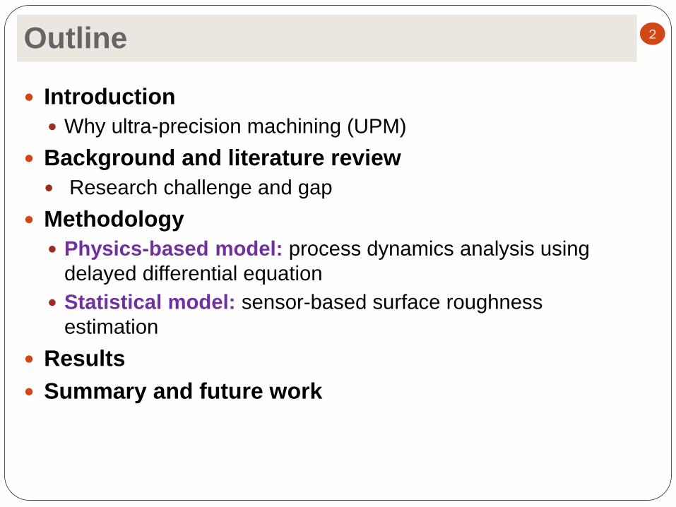
Outline

Introduction

Why ultra-precision machining (UPM)

Background and literature review

Research challenge and gap

Methodology

Physics-based model: process dynamics analysis using

delayed differential equation

Statistical model: sensor-based surface roughness

estimation

Results

Summary and future work

2

Introduction

Development of sensor-based technique: especially in

advanced manufacturing processes control

Aerospace, biomedical, electronics, automotive et al. (Lee 1999,

Liu 2004)

Taniguchi curve: nano-metric manufacturing accuracy

Industry relies on ultra-precision machining (UPM) to realize

surface roughness (Ra) at 10 nm – 30 um

3

Taniguchi 1983

Challenge in UPM 4

Quality issue: anomaly development (even in well-designed process) cannot be predicted

Physics-based models: cannot predict surface change

Cutting mechanics: cutting stresses (Marsh 2005); micro-plasticity effect (Yuan 1994, Lee 2001); tool interference (Cheung 2003);

material recovery and swelling effect (Kong 2006)

Micro-physics: crystallographic orientation of the grain (Lee

2000); metrology and process physics (Dornfeld et al. 2006)

Spectrum analysis: Ra spectrum component (Cheung and Lee

2000, Pandit and Shaw 1981, Hocheng et al. 2004)

Prahalad 2013 High-definition optical inspection

Surface roughness models

Sensor-based analytics models: applicable for real-time

Ra estimation

Vibration analysis: vibration amplitude and frequency (Lin 1998,

Abouelatta and Madl 2001, Liu 2004)

Acoustic emission (Beggan et al. 1999)

Temperature sensor (Hayashi et al. 2008)

Strain gauge sensor (Shinno et al. 1997)

Limited by nonlinear and nonstationary nature of machining

signals

5

Cheng et al. 2014

Approach

Physics domain model: consider tool radius effect,

ploughing and shearing effect, elastic material recovery; predict

system dynamic response

Sensor-based model: extract information from in situ

signals; detect change in the process

6

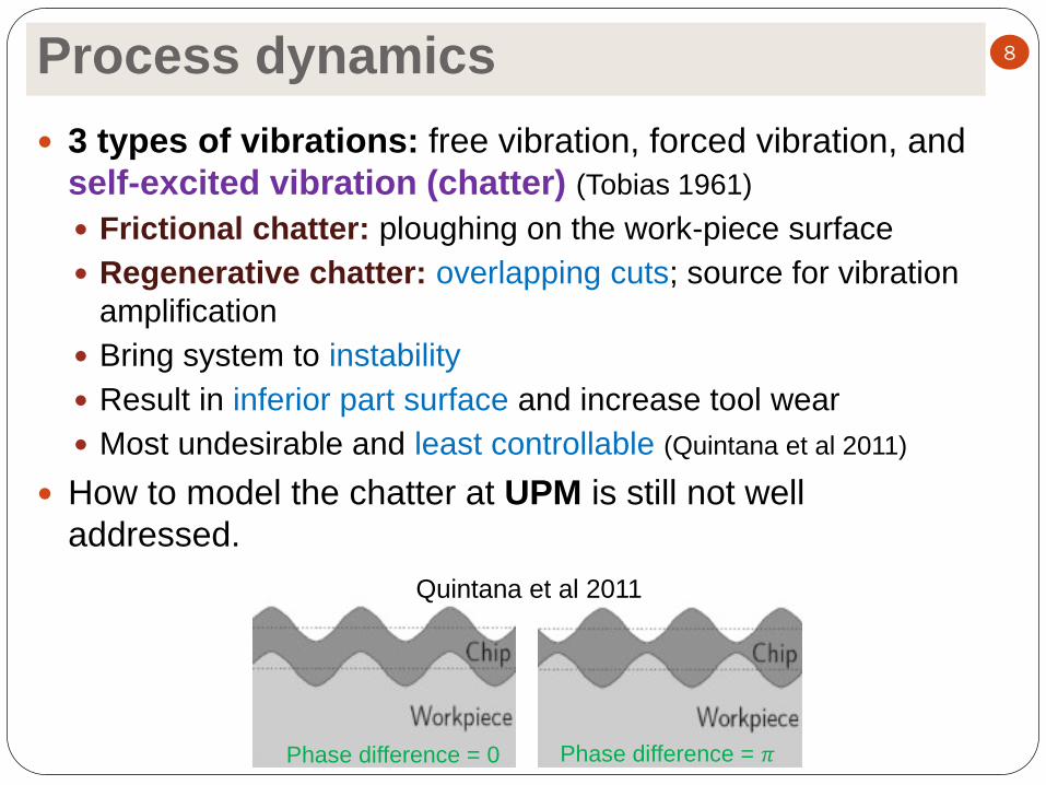
Process dynamics

3 types of vibrations: free vibration, forced vibration, and

self-excited vibration (chatter) (Tobias 1961)

Frictional chatter: ploughing on the work-piece surface

Regenerative chatter: overlapping cuts; source for vibration

amplification

Bring system to instability

Result in inferior part surface and increase tool wear

Most undesirable and least controllable (Quintana et al 2011)

How to model the chatter at UPM is still not well

addressed.

8

Phase difference = 0 Phase difference = 𝜋

Quintana et al 2011

UPM dynamics model

𝑦 𝑡 + 2휁𝜔𝑛𝑦 𝑡 + 𝜔𝑛2𝑦 𝑡 = −

𝐹 𝑦 𝑡 ,𝑦 𝑡−𝑇

𝑚

𝑦: tool displacement

𝑇: period length, 𝑇 =1

Ω

Process parameters: feed 𝑓0, spindle speed Ω, chip width 𝑤

Thrust force model: shearing and ploughing components

9

𝑓0 ≥ 𝑓𝑚𝑖𝑛: material removal; both

shearing and ploughing forces exist

𝑓0 < 𝑓𝑚𝑖𝑛 : only elastic deformation

and ploughing force

𝑓0

Shearing Force

Dynamic chip thickness

𝑡𝑢 = (𝑓0 − 𝑦 𝑡 + 𝑦(𝑡 − 𝑇)) − 𝛿

Shearing angle (Waldorf et al 1999)

10

𝜙 = tan−1𝑓0 − 𝛿

𝑅tan𝜋4+

𝛼2

+𝛿

tan(𝜋2+ 𝛼)

− 2𝑅𝛿 − 𝛿2 + 𝑡𝑐/ cos 𝛼 − 𝑓0 tan 𝛼

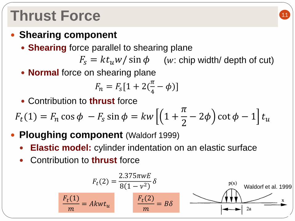
Thrust Force

Shearing component

Shearing force parallel to shearing plane

(𝑤: chip width/ depth of cut)

Normal force on shearing plane

𝐹𝑛 = 𝐹𝑠[1 + 2(𝜋

4− 𝜙)]

Contribution to thrust force

𝐹𝑡(1) = 𝐹𝑛 cos 𝜙 − 𝐹𝑠 sin𝜙 = 𝑘𝑤 1 +𝜋

2− 2𝜙 cot 𝜙 − 1 𝑡𝑢

Ploughing component (Waldorf 1999)

Elastic model: cylinder indentation on an elastic surface

Contribution to thrust force

11

𝐹𝑠 = 𝑘𝑡𝑢𝑤/ sin𝜙

𝐹𝑡(1)

𝑚= 𝐴𝑘𝑤𝑡𝑢

Waldorf et al. 1999 𝐹𝑡(2) =

2.375𝜋𝑤𝐸

8 1 − 𝜈2 𝛿

𝐹𝑡(2)

𝑚= 𝐵𝛿

Process dynamics

Delayed differential equation for tool dynamics

𝑦 𝑡 + 2휁𝜔𝑛𝑦 𝑡 + 𝜔𝑛2𝑦 𝑡 = −

𝐹𝑡(1) + 𝐹𝑡(2)

𝑚= −𝐴𝑡𝑢 − 𝐵𝛿

= −𝐴𝑘𝑤𝑓0 − 𝐴𝑘𝑤 𝑦 𝑡 − 𝑦 𝑡 − 𝑇 + 𝛿 𝐴𝑘𝑤 − 𝐵= −𝐴𝑘𝑤 𝑦 𝑡 − 𝑦 𝑡 − 𝑇 + 𝐶

No closed-form solution to dynamics state: 𝑦(𝑡)

Temporal finite element model can be used for

approximation (Bayly et al. 2003, Khasawneh et al. 2009)

The time per revolution 𝑻 is divided into 𝑴 elements

Approximation to the solution for the tool displacement on

each element

𝑦𝑗𝑛 𝜏 = 𝑎𝑗𝑖

𝑛𝑆𝑖(𝜏) 4𝑖=1 𝑦𝑗

𝑛−1 𝜏 = 𝑎𝑗𝑖𝑛−1𝑆𝑖(𝜏)

4𝑖=1

𝜏: local time, 0 ≤ 𝜏 ≤ 𝑡𝑗; 𝑡𝑗: time for element 𝑗, 𝑡𝑗 =𝑇

𝑀

12

Temporal finite element model (TFEM)

Hermite basis functions (Mann et al. 2006)

13

Displacement: 𝑎11 𝑎13/𝑎21 𝑎23

𝑆1 𝜏 = 1 − 3𝜏

𝑡𝑗

2

+ 2𝜏

𝑡𝑗

3

𝑆2 𝜏 = 𝑡𝑗𝜏

𝑡𝑗− 2

𝜏

𝑡𝑗

2

+𝜏

𝑡𝑗

3

𝑆3 𝜏 = 3𝜏

𝑡𝑗

2

− 2𝜏

𝑡𝑗

3

𝑆4 𝜏 = 𝑡𝑗 −𝜏

𝑡𝑗

2

+𝜏

𝑡𝑗

3

• Orthogonal; second-order

continuous

• Coefficients represent the state

variable (displacement and

velocity) at the beginning/end of

each element

• Boundary conditions

Velocity: 𝑎12 𝑎14/𝑎22 𝑎24

TFEM

Approximation leads to non-zero error

𝑎𝑗𝑖𝑛𝜙 𝑖

4

𝑖=1

+ 2휁𝜔𝑛 𝑎𝑗𝑖𝑛𝜙 𝑖

4

𝑖=1

+ 𝜔𝑛2 𝑎𝑗𝑖

𝑛𝜙𝑖

4

𝑖=1

+ 𝐴𝑘𝑤 𝑎𝑗𝑖𝑛𝜙𝑖

4

𝑖=1

− 𝑎𝑗𝑖𝑛−1𝜙𝑖

4

𝑖=1

− 𝐶 = 𝑒𝑟𝑟𝑜𝑟

Method of weighted residuals (Reddy 1993)

Independent trial functions: 𝜓1 = 1 𝜓2 =2𝜏

𝑡𝑗− 1

𝑎𝑗𝑖𝑛𝜙 𝑖

4

𝑖=1

+ 2휁𝜔𝑛 𝑎𝑗𝑖𝑛𝜙 𝑖

4

𝑖=1

+ 𝜔𝑛2 𝑎𝑗𝑖

𝑛𝜙𝑖

4

𝑖=1

𝑡𝑗

0

+ 𝐴𝑘𝑤 𝑎𝑗𝑖𝑛𝜙𝑖

4

𝑖=1

− 𝑎𝑗𝑖𝑛−1𝜙𝑖

4

𝑖=1

− 𝐶 𝜓𝑝 𝜏 𝑑𝜏 = 0

14

TFEM

𝑎𝑗𝑖𝑛 𝜙 𝑖 + 2휁𝜔𝑛𝜙 𝑖 + 𝜔𝑛

2 + 𝐴𝑘𝑤 𝜙𝑖

𝑡𝑗

0

4

𝑖=1

𝜓𝑝 𝜏 𝑑𝜏

= 𝑎𝑗𝑖𝑛−1 𝐴𝑘𝑤𝜙𝑖

𝑡𝑗

0

4

𝑖=1

𝜓𝑝 𝜏 𝑑𝜏 + 𝐶𝜓𝑝 𝜏 𝑑𝜏 𝑡𝑗

0

15

𝑎𝑗𝑖𝑛

4

𝑖=1

𝑁𝑝𝑖𝑗

= 𝑎𝑗𝑖𝑛−1𝑃𝑝𝑖

𝑗

4

𝑖=1

+ 𝑄𝑝𝑗

𝑃𝑝𝑖𝑗

= 𝐴𝑘𝑤𝜙𝑖

𝑡𝑗

0

𝜓𝑝 𝜏 𝑑𝜏

𝑄𝑝𝑗= 𝐶𝜓𝑝 𝜏 𝑑𝜏

𝑡𝑗0

𝑁𝑝𝑖𝑗

= 𝜙 𝑖 + 2휁𝜔𝑛𝜙 𝑖 + 𝜔𝑛2 + 𝐴𝑘𝑤 𝜙𝑖

𝑡𝑗

0

TFEM

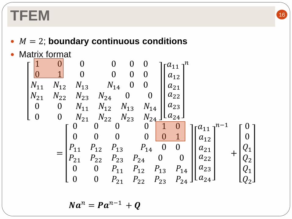
𝑀 = 2; boundary continuous conditions

Matrix format 1 0 00 1 0

𝑁11 𝑁12 𝑁13

0 0 00 0 0

𝑁14 0 0𝑁21 𝑁22 𝑁23

0 0 𝑁11

0 0 𝑁21

𝑁24 0 0𝑁12 𝑁13 𝑁14

𝑁22 𝑁23 𝑁24

𝑎11 𝑎12

𝑎21𝑎22

𝑎23

𝑎24

𝑛

=

0 0 00 0 0

𝑃11 𝑃12 𝑃13

0 1 00 0 1

𝑃14 0 0𝑃21 𝑃22 𝑃23

0 0 𝑃11

0 0 𝑃21

𝑃24 0 0𝑃12 𝑃13 𝑃14

𝑃22 𝑃23 𝑃24

𝑎11 𝑎12

𝑎21𝑎22

𝑎23

𝑎24

𝑛−1

+

00𝑄1

𝑄2

𝑄1

𝑄2

𝑵𝒂𝑛 = 𝑷𝒂𝑛−1 + 𝑸

16

Stability analysis

𝒂𝑛 = 𝑮𝒂𝑛−1 + 𝑵−1𝑸 (𝑮 = 𝑵−1𝑷 Monodromy operator )

Criterion: asymptotic stability requires eigenvalues of

𝑮 within the unit circle of the complex plane

Maximum absolute eigenvalues< 𝟏

Stability lobe diagram

Map the area of stability as a function of the machining

parameters (feed, depth of cut, and spindle speed)

Identify the optimum conditions that maximize the chatter-

free material removal rate and avoid inferior surface

17

Sensitivity analysis

Stability sensitivity on 𝛿 with perturbation 𝑑𝛿

tan𝜙′ = tan𝜙 + −𝑅 tan𝜋

4+

𝛼

2−

𝑡𝑐cos 𝛼

+ 𝑓0 cot 𝛼 +𝑓0𝑅 + 𝑅 − 𝑓0 𝛿

2𝑅𝛿 − 𝛿2𝑑𝛿

𝐴′ ≈1 +

𝜋2

tan𝜙+

2 tan𝜙 2

3− 3

+2 tan𝜙 (𝑓0𝑅 + 𝑅 − 𝑓0 𝛿)

3 2𝑅𝛿 − 𝛿2−

(1 +𝜋2)(𝑓0𝑅 + 𝑅 − 𝑓0 𝛿)

2𝑅𝛿 − 𝛿2 tan𝜙 2𝑑𝛿

18

𝐶0 ≪ tan𝜙, 𝐶0 = 0

Sensitivity analysis

2-element maximum eigenvalue analysis

𝜆′𝑚𝑎𝑥 ≈ 𝜆𝑚𝑎𝑥 +tan 𝜙′ 2

tan 𝜙+𝑓0𝑅+ 𝑅−𝑓0 𝛿

2𝑅𝛿−𝛿2𝑑𝛿

1+2𝜋

4−𝜙′

𝑡𝑎𝑛𝜙′− 1 1 +

𝜋

2+

tan 𝜙 2𝑅𝛿−𝛿2

1+𝜋

2𝑓0𝑅+ 𝑅−𝑓0 𝛿

𝑑𝛿

Given 𝑑𝛿 = ±0.2𝛿, 𝜆𝑚𝑎𝑥′ ≈ 𝜆𝑚𝑎𝑥 ± 0.08

Uncertainty for stability boundary: 𝜆𝑚𝑎𝑥 close to 1

19

UPM experiment setup

Face turning of aluminum alloy disk-shaped workpiece

Cutting tools: polycrystalline diamond (𝑅 = 60 𝑢𝑚)

Vibration sensors: Kistler 8782A500

Force sensors: 3-axis piezoelectric dynamometer Kistler

A9251A

20

Cutting Force Sensors

Marks on sample

Cutting Tool

Acoustic Emission Sensor

Vibration Sensors

Feed = 12 / 6 um per revolution 21

• 𝑅𝑎 measured from MicroXAM® for chatter identification

• 𝑅𝑎 > 100 𝑛𝑚: onset of the chatter

Feed = 3 / 1.5 um per revolution 22

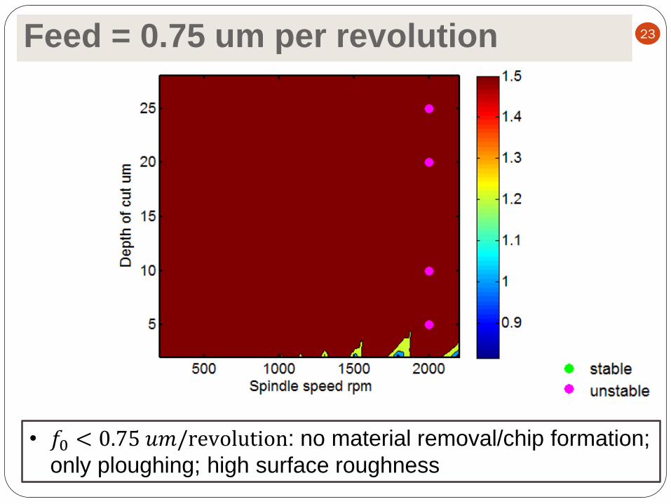
Feed = 0.75 um per revolution 23

• 𝑓0 < 0.75 𝑢𝑚/revolution: no material removal/chip formation;

only ploughing; high surface roughness

Summary for physics-based model

Delayed differential equation (DDE) with temporal finite

element model (TFEM)

Investigate the process dynamics for UPM

Consider the dynamic shearing and ploughing forces at

nano-scale machining

Can identify optimum conditions, tending to generate low

surface roughness

Challenges

Surface roughness Ra varies according to chip formation

process and other uncontrollable factors even under

optimum conditions

Ra variation monitoring in the incipient stages in real-time

given process parameters; vital for nano-metric range finish

assurance

24

Physics-based sensor fusion technique for Ra real-time estimation

Sensor-based model

Feature extraction

Difficult to evaluate UPM process from the raw time series

signals

Transform time series into feature space with reliable,

effective and accurate features

Identify the patterns hidden into the raw signals

25

Statistical features 26

State space reconstruction 27 Recurrence quantification analysis

𝑥 Nonlinear vibration signal

Recurrence quantification analysis

Threshold recurrence plot

RQA extraction

Nonlinear Dynamic Characterization

Time delay 𝜏

Embedded dimension 𝑑

State space

reconstruction

𝑋

PCA

Total number of variables: 3 + 6 × 9 = 57

The first 3 principal components explained over 70% of

the total variance

Contribution to the 1st principal component

28

𝑉𝑖𝑏_𝑋

𝑉𝑖𝑏_𝑌 𝐹_𝑋 𝐹_𝑍

Gaussian process (GP) model

Mapping between input 𝑠 ∈ 𝑅𝑛𝑝 and z ∈ 𝑅

z = 𝑓 𝑠 + 휀 휀 ∼ 𝑁(0, 𝜎12)

Without explicit functional form, covariance structure can be used to represent the function value distribution

Z ∼ 𝑁(0, 𝐾 𝑆, 𝑆 + 𝜎12𝐼)

𝑋 = 𝑠1, 𝑠2, … , 𝑠𝑛𝑝 and 𝑍 = [𝑧1, 𝑧2, … , 𝑧𝑛𝑝

]

Covariance matrix 𝐾𝑖𝑗 = 𝑘𝜃(𝑠𝑖 , 𝑠𝑗), 𝜃 hyperparameters to be estimated

Squared exponential form

𝑘𝜃 𝑠𝑖 , 𝑠𝑗 = 𝜎02 exp −

(𝑠𝑖−𝑠𝑗)𝑇𝑀(𝑠𝑖−𝑠𝑗)

2+ 𝜎1

2

𝜎02: process variance

𝜎12: noise variance

𝑀 = 𝑑𝑖𝑎𝑔 𝑙 −2: length scale in each input direction

Infinitely differentiable; close points are highly correlated

Log likelihood function to optimize the hyperparameters

29

GP prediction

At new input 𝑠∗ ∈ 𝑅𝑛𝑝 , the noise-free prediction 𝑓∗ is given

by the first two moments

Can predict a complete distribution 𝐾 𝑆, 𝑠∗ : 𝑛𝑝 × 1 vector, each element is the covariance

between 𝑠∗ and one sample point

Mean: linear combination of the observation values

Covariance: difference between prior covariance and the

information explained

30

),()),((),(),()cov(

)),((),(

*

12

1****

12

1**

sSKISSKsSKssKf

ZISSKsSKf

T

T

30

Estimation result 31

Accuracy of the fitting

Over 85% of measured Ra values are within the 2-sigma

prediction band

Summary and future work

Summary

Physics-based model can predict chatter onset according

to process parameters; not applicable for real-time Ra

estimation

Physics-based statistical model can estimate the surface

roughness with accuracy over 80%

Future work

Cutting speed and thermal effects on the thrust force

Built-up edge effect: dead metal cap on tool edge

Uncertainty in the stability analysis

32

Acknowledgement

We acknowledge the generous support of the NSF

(Grants CMMI 100978, 1301439).

33