0

Dynamics of Rural Poverty in Pakistan:

Evidence from Three Waves of the Panel

Survey

G. M. Arif and Shujaat Farooq

July 2012

Pakistan Institute of Development Economics

Islamabad

1

Dynamics of Rural Poverty in Pakistan: Evidence from Three Waves of the

Panel Survey

G. M. Arif and Shujaat Farooq1

1. Introduction

Poverty analysis in developing countries including Pakistan has in general focused on poverty trends

based on cross-sectional datasets, with very little attention being paid to its dynamics – that is transitory

or chronic poverty. Transitory poor are those who move out or fall into poverty between two periods

whereas the chronic poor remain in the poverty trap for a significant period of their lives. The static

measures of households‟ standard of living do not necessarily provide a good insight to their likely

stability over time. For instance, a high mobility into or out of poverty may suggest that a higher

proportion of a population experiences poverty over time than what the cross-sectional data might show2.

It also implies that a much smaller proportion of the population experiences chronic poverty relative to

those poor who are enumerated on cross-sectional observations in a particular year (Hossain and Bayes,

2010). Thus, the analysis of poverty dynamics is important to uncover the true nature of wellbeing of

population. Both the micro and macro level socio-demographic and economic factors are likely to affect

poverty movements and intergenerational poverty transmission (Krishna, 2011).

A close look at the data on poverty levels and trends in Pakistan for the last five decades leads to two

broad conclusions: first, poverty reduction has not been sustainable rather than it has fluctuated

remarkably; and second, a large proportion of the population has been found around the poverty line, and

any micro and/or macro shock (positive or negative) is likely to push them into poverty or to pull them

out of it. But this dynamism of poverty is generally not addressed in poverty reduction strategies of the

country. The reason is that although the existing poverty literature in Pakistan is prolific in descriptive

studies based on the cross-sectional household surveys such as the Household Income and Expenditure

Survey (HIES), studies on poverty dynamics, which need longitudinal datasets, are scant.

1 G.M. Arif is Joint Director at the Pakistan Institute of Development Economics (PIDE) while Shujaat Farooq is

Assistant Professor at the National University for Science and Technology (NUST), Islamabad. They are thankful to

Dr. Rashid Amjad, Vice Chancellor, PIDE, for his guidance and support to complete the panel survey and this

research. They are also thankful to Dr. Durr-e-Nayab, Chief of Research, PIDE, for her valuable comments on the

earlier draft. 2 See for example, Adelman et al. (1985), Gaiha and Deolalikar, (1993) for India; Jalan and Ravallion (2001) for

China; Sen (2003) and Hossain and Bayes (2010) for Bangladesh; Kurosaki (2006), Arif and Bilquees (2007),

Lohano (2009) and Arif et al. (2011) for Pakistan.

2

The few available studies on poverty dynamics in Pakistan have generally been based on two rounds of a

panel household survey.3 Their contribution in knowledge is substantial, but data on more rounds (waves)

uncover the dynamics more effectively. For example, the incidence of chronic poverty has generally been

higher in two-round surveys than in surveys which had more than two rounds, suggesting that there could

be only a small proportion of population that remains in the state of poverty for extended period of time.

Effective and right policies, based on the philosophy of inclusiveness, can, thus, at least alleviate chronic

poverty from the country, which could be a big socio-economic achievement for a developing country

like Pakistan.

The major objective of this study is to analyze the dynamics of rural poverty in Pakistan using the three

waves of a panel household survey carried out by the Pakistan Institute of Development Economics

(PIDE) in 2001, 2004 and 2010. This analysis of dynamics in poverty is important from both the micro

and macro perspectives. In micro-perspective, demographic dynamics and change in household asset

status may have an impact on the poverty movements. Similarly, the macroeconomic situation, which

fluctuated remarkably during the 2001 to 2010 period - moderate growth during the first six years of

2000s and sluggish growth with double-digit inflation particularly the food inflation since 2007 - is likely

to have affected a household‟s well-being. The two natural major disasters during the 2005-10 period,

earthquake and flood, may also have lasting impact on the living standard of population.

The rest of the paper is organized as follows. A brief review of the literature on dynamics of poverty has

been presented in section 2, followed by a discussion on the data sources and analytical framework in

section 3. Section 4 reports changes in the household demographic and socio-economic characteristics

during the three rounds of the panel survey. Cross-sectional poverty estimates and its determinants have

been discussed in section 5. Dynamics of rural poverty and its determinants are examined in sections 6

and 7 respectively. Conclusions are given in the final section.

2. A Brief Literature Review

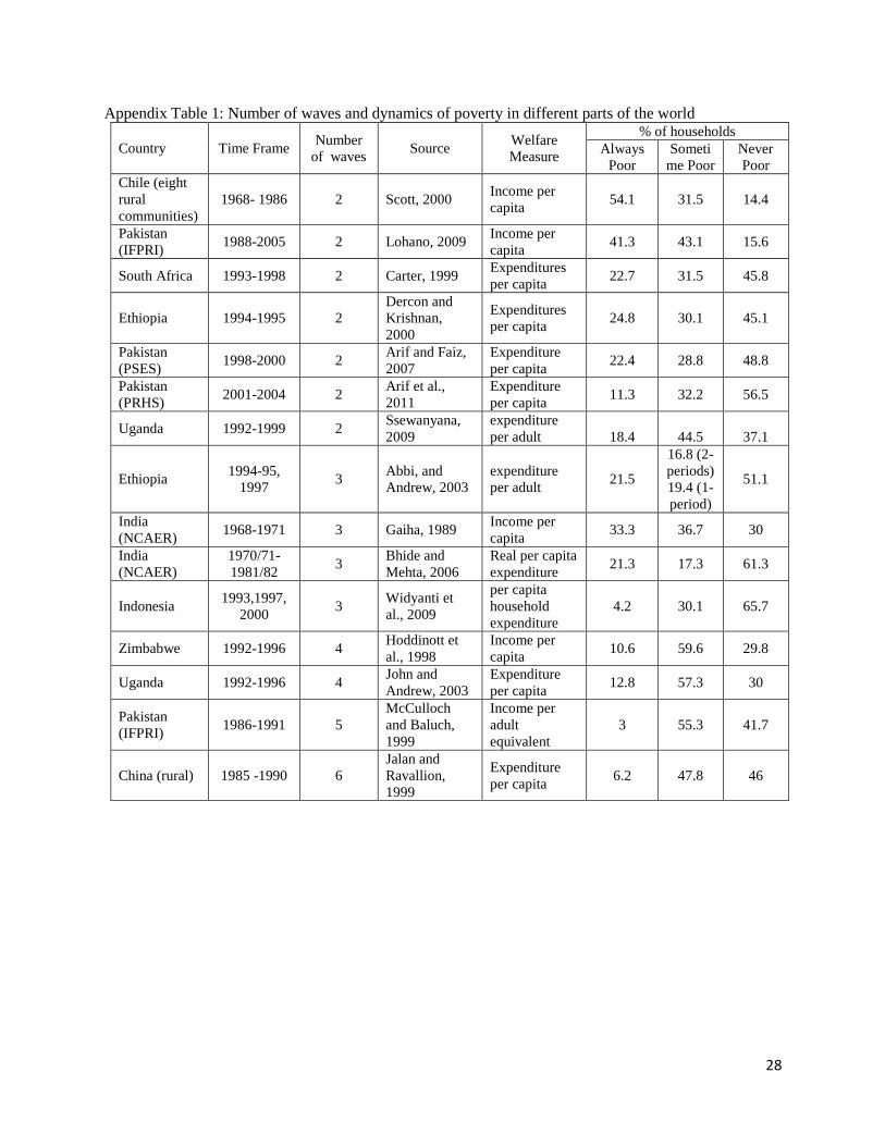
The findings of poverty dynamics studies carried out in different parts of the world during last four

decades are summarized in Appendix Table 1. The „never poor‟ category shown in the last column of this

Table shows the percentage of households (or population) that did not experience any episode of poverty

during the different waves of the respective surveys. In contrast, the „always poor‟ category in the Table

represents the chronic poverty, proportion of households (or population) that remained poor in all rounds

of the respective surveys. It is not possible from the data in Table 1 to find out a direct association

between the number of waves and the proportion of households in the „never poor‟ category or in „always

3 Kurosaki (2006), Arif and Bilquees (2007), Lohano (2009) and Arif et al. (2011)

3

poor‟ category. However, the data do show that as the number of waves increases, the proportion of

chronic poor (always poor) as well as „never poor‟ in general declines with a corresponding increase in

the transitory poverty (poor sometime).

The literature has identified several factors associated with the dynamics of poverty. The changing socio-

demographic and economic characteristics of the household have been considered as the key drivers of

chronic and transient poverty. Regarding the demographic characteristics, larger household size and/or

dependency ratio are associated with chronic poverty as it put an extra burden on a household‟s assets and

resource base (Jayaraman and Findeis, 2005; Ssewanyana, 2009). Changes in household size and age

structures (young, adult and elderly) are also linked with the movements into and out of poverty because

of their distinct economic consequences (Bloom et al, 2002). Additional children not only raise the

likelihood of a household to fall into poverty but it also lead to intergenerational transmission of poverty

due to reduction in school attendance of children with a regressive impact on poorer households (Orbeta,

2005). Households headed by female are more likely to be chronically poor (John and Andrew, 2003);

majority of these women are serially dispossessed (divorced then widowed), therefore, may promote

intergenerational poverty (Corta and Magongo, 2011). The male-oriented customary inheritance system

also makes the female at disadvantageous position (Miller et al., 2011).

A number of studies have shown that the increase in human capital reduces the likelihood of being

chronic poor or transient poor. Such evidence from literature has been seen in the milieu of the education

of the head of the household (Wlodzimierz, 1999; Arif et al., 2011) as well as the education of the

children to overcome the persistent poverty (Davis, 2011). However, only formal education does not

matter; the innate disadvantages and lack of skills are also significantly associated with chronic poverty

(Grootaert et al. 1997). Regarding health, the inadequate dietary intake triggers off a chain reaction,

leading to the loss of body weight and mutilation of physical growth, especially among children (Hossain

and Bayes, 2010). The households that have a permanent disable person are relatively more likely to face

persistent poverty (Krishna, 2011).

Both the chronic and transient poverty are closely associated with the tangible and less-tangible

composition of assets of the households (Davis, 2011). It can be viewed in terms of land ownership (Jalan

and Ravallion, 2000; Arif et al., 2011), livestock ownership (Davis, 2011), possession of liquid assets

(Wlodzimierz, 1999), remittances (Arif et al., 2011) and access to water, sanitation, electricity and ability

to effectively invest on land (Cooper, 2010). Mobility in land ownership is highly linked with the

transient poverty (Hossain and Bayes, 2010); the amount of received land from parents is a significant

predictor to remain non-poor (Davis, 2011). Location also plays a vital role in the opportunities available

to households. The households living in remote areas with less infrastructure and other basic facilities are

4

more likely to be chronic and transient poor (Arif et al., 2011; Deshingkar, 2010). Asset-less households

are more likely to fall into poverty if the economy is not doing well and/or the distribution of assets is

highly unequal (Hossain and Bayes, 2010). The land distribution is highly skewed in Pakistan even more

than income (Hirashima, 2009) as about 63 percent of the rural households are landless while only 2

percent of the rural households owned 50 acres or more, accounting for 30 percent of the total land

(World Bank, 2007).

Households face a variety of risks and shocks i.e. macroeconomic shock, inflation, natural disaster, health

hazard, personal insecurity, and socially compulsive expenses such as dowry. The customary and

ceremonial expenses on marriages and funerals may sometime push the households into a long-term

poverty (Krishna, 2011). Using a six wave dataset from rural China, Jalan and Ravallion (2001) found a

significant fall in household consumption followed by a shock; higher the severity of the shock, more the

time would be taken to recover from it. In agriculture regions, loss of land, floods and lack of irrigation

system also push households into poverty (Sen, 2003). The poor households had poor quality land, poorer

resource base (Singh and Binswanger, 1993). Based on life history analysis in rural Bangladesh, Davis

(2011) found that a variety of shocks at various horizons of the life determine the pattern of transient and

intergenerational transmission of poverty; the accumulation of physical and soft assets as well as the

location is one of the most important means by which poor people in rural Bangladesh improve their

lives.

3. Data sources and Analytical Framework

Three waves of a panel dataset have been used in this study. The first two rounds of the panel survey

named as „Pakistan Rural Household Survey‟ (PRHS) were carried out in 2001 and 2004 only in rural

areas. In the third round, which was conducted in 2010, an urban sample was also included, and it was re-

named as „Pakistan Panel Household Survey‟ (PPHS). The PRHS-2001 was conducted in all four

provinces of the country while, due to security concerns, the PRHS-2004 was restricted to two large

provinces, Punjab and Sindh. The PPHS-2010 has again covered all the four provinces, so the left-over

households of Khyber PakhtunKhwa (KP) and Balochistan were re-interviewed after ten years in 2010.

The urban sample for the PPHS 2010 was selected from those 16 districts that were included in the first

round (PRHS 2001). These 16 districts are: Attock, Faisalabad, Hafizabad, Vehari, Muzaffargarh and

Bahawalpur in Punjab; Badin, Mirpur Khas, Nawabshah and Larkana in Sindh; Dir, Mardan and Lakki

Marwat in KP; and Loralai, Khuzdar and Gwader in Balochistan.

Table 1 shows the sample size of all three rounds of the panel survey and it also includes the split

households covered in both 2004 and 2010 rounds. A split household is a new household where at least

5

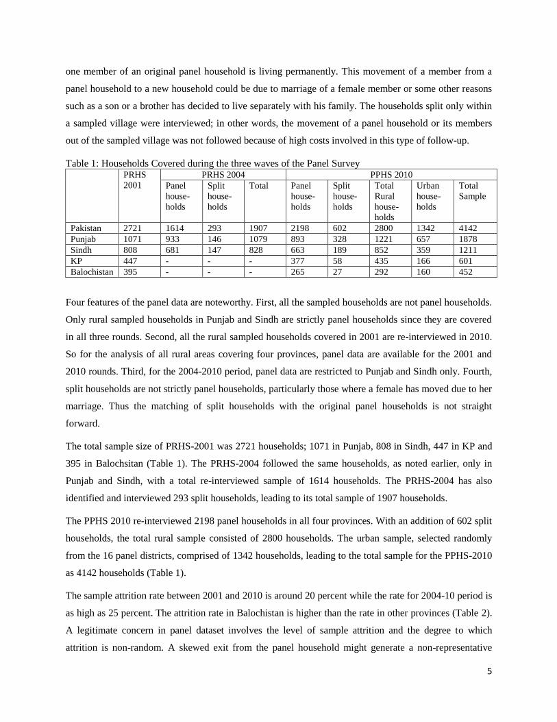
one member of an original panel household is living permanently. This movement of a member from a

panel household to a new household could be due to marriage of a female member or some other reasons

such as a son or a brother has decided to live separately with his family. The households split only within

a sampled village were interviewed; in other words, the movement of a panel household or its members

out of the sampled village was not followed because of high costs involved in this type of follow-up.

Table 1: Households Covered during the three waves of the Panel Survey PRHS

2001

PRHS 2004 PPHS 2010

Panel

house-

holds

Split

house-

holds

Total Panel

house-

holds

Split

house-

holds

Total

Rural

house-

holds

Urban

house-

holds

Total

Sample

Pakistan 2721 1614 293 1907 2198 602 2800 1342 4142

Punjab 1071 933 146 1079 893 328 1221 657 1878

Sindh 808 681 147 828 663 189 852 359 1211

KP 447 - - - 377 58 435 166 601

Balochistan 395 - - - 265 27 292 160 452

Four features of the panel data are noteworthy. First, all the sampled households are not panel households.

Only rural sampled households in Punjab and Sindh are strictly panel households since they are covered

in all three rounds. Second, all the rural sampled households covered in 2001 are re-interviewed in 2010.

So for the analysis of all rural areas covering four provinces, panel data are available for the 2001 and

2010 rounds. Third, for the 2004-2010 period, panel data are restricted to Punjab and Sindh only. Fourth,

split households are not strictly panel households, particularly those where a female has moved due to her

marriage. Thus the matching of split households with the original panel households is not straight

forward.

The total sample size of PRHS-2001 was 2721 households; 1071 in Punjab, 808 in Sindh, 447 in KP and

395 in Balochsitan (Table 1). The PRHS-2004 followed the same households, as noted earlier, only in

Punjab and Sindh, with a total re-interviewed sample of 1614 households. The PRHS-2004 has also

identified and interviewed 293 split households, leading to its total sample of 1907 households.

The PPHS 2010 re-interviewed 2198 panel households in all four provinces. With an addition of 602 split

households, the total rural sample consisted of 2800 households. The urban sample, selected randomly

from the 16 panel districts, comprised of 1342 households, leading to the total sample for the PPHS-2010

as 4142 households (Table 1).

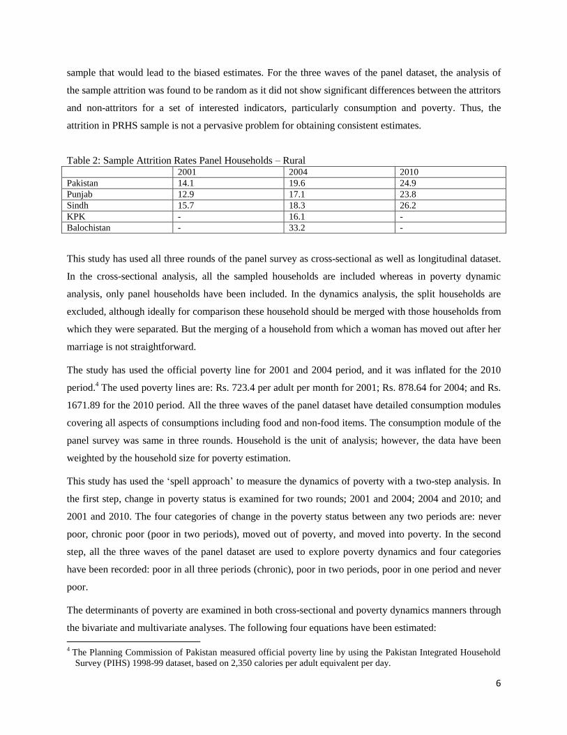
The sample attrition rate between 2001 and 2010 is around 20 percent while the rate for 2004-10 period is

as high as 25 percent. The attrition rate in Balochistan is higher than the rate in other provinces (Table 2).

A legitimate concern in panel dataset involves the level of sample attrition and the degree to which

attrition is non-random. A skewed exit from the panel household might generate a non-representative

6

sample that would lead to the biased estimates. For the three waves of the panel dataset, the analysis of

the sample attrition was found to be random as it did not show significant differences between the attritors

and non-attritors for a set of interested indicators, particularly consumption and poverty. Thus, the

attrition in PRHS sample is not a pervasive problem for obtaining consistent estimates.

Table 2: Sample Attrition Rates Panel Households – Rural 2001 2004 2010

Pakistan 14.1 19.6 24.9

Punjab 12.9 17.1 23.8

Sindh 15.7 18.3 26.2

KPK - 16.1 -

Balochistan - 33.2 -

This study has used all three rounds of the panel survey as cross-sectional as well as longitudinal dataset.

In the cross-sectional analysis, all the sampled households are included whereas in poverty dynamic

analysis, only panel households have been included. In the dynamics analysis, the split households are

excluded, although ideally for comparison these household should be merged with those households from

which they were separated. But the merging of a household from which a woman has moved out after her

marriage is not straightforward.

The study has used the official poverty line for 2001 and 2004 period, and it was inflated for the 2010

period.4 The used poverty lines are: Rs. 723.4 per adult per month for 2001; Rs. 878.64 for 2004; and Rs.

1671.89 for the 2010 period. All the three waves of the panel dataset have detailed consumption modules

covering all aspects of consumptions including food and non-food items. The consumption module of the

panel survey was same in three rounds. Household is the unit of analysis; however, the data have been

weighted by the household size for poverty estimation.

This study has used the „spell approach‟ to measure the dynamics of poverty with a two-step analysis. In

the first step, change in poverty status is examined for two rounds; 2001 and 2004; 2004 and 2010; and

2001 and 2010. The four categories of change in the poverty status between any two periods are: never

poor, chronic poor (poor in two periods), moved out of poverty, and moved into poverty. In the second

step, all the three waves of the panel dataset are used to explore poverty dynamics and four categories

have been recorded: poor in all three periods (chronic), poor in two periods, poor in one period and never

poor.

The determinants of poverty are examined in both cross-sectional and poverty dynamics manners through

the bivariate and multivariate analyses. The following four equations have been estimated:

4 The Planning Commission of Pakistan measured official poverty line by using the Pakistan Integrated Household

Survey (PIHS) 1998-99 dataset, based on 2,350 calories per adult equivalent per day.

7

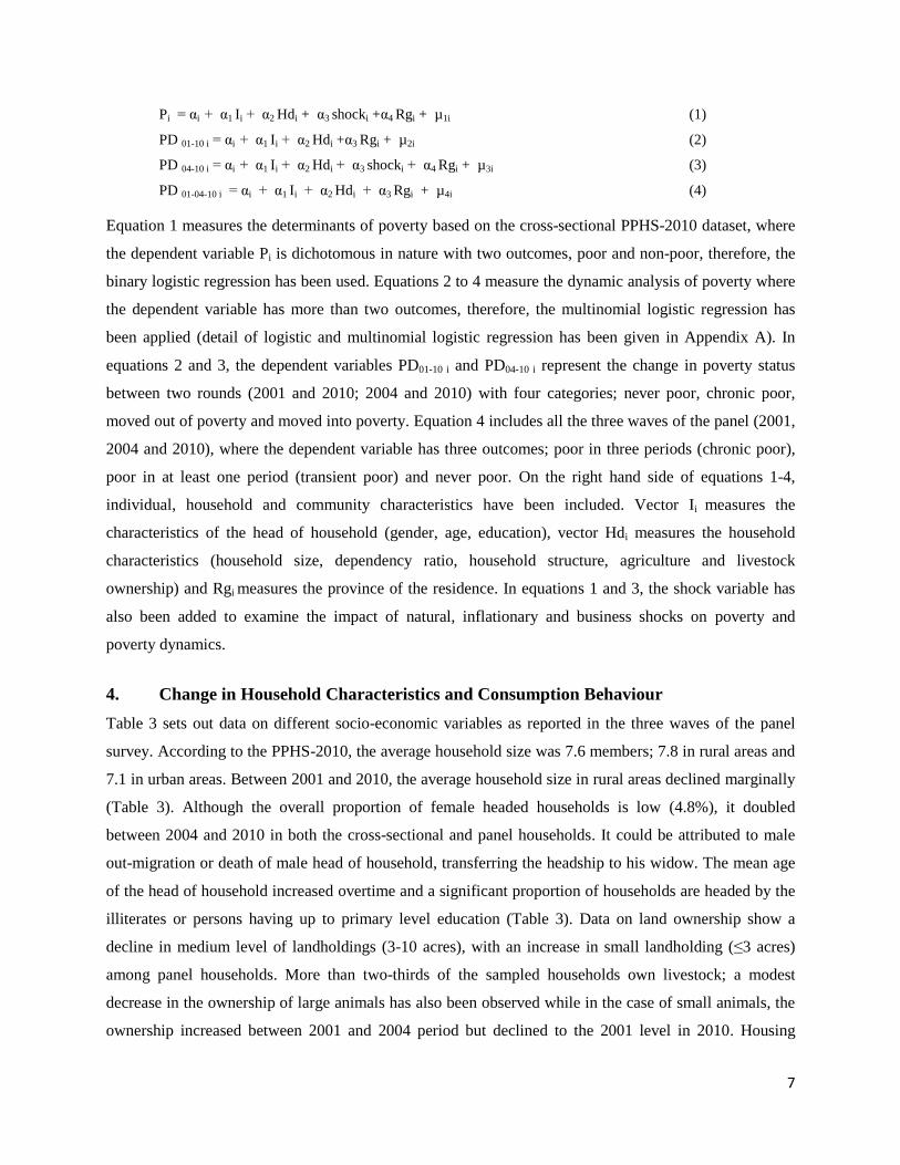
Pi = αi + α1 Ii + α2 Hdi + α3 shocki +α4 Rgi + µ1i (1)

PD 01-10 i = αi + α1 Ii + α2 Hdi +α3 Rgi + µ2i (2)

PD 04-10 i = αi + α1 Ii + α2 Hdi + α3 shocki + α4 Rgi + µ3i (3)

PD 01-04-10 i = αi + α1 Ii + α2 Hdi + α3 Rgi + µ4i (4)

Equation 1 measures the determinants of poverty based on the cross-sectional PPHS-2010 dataset, where

the dependent variable Pi is dichotomous in nature with two outcomes, poor and non-poor, therefore, the

binary logistic regression has been used. Equations 2 to 4 measure the dynamic analysis of poverty where

the dependent variable has more than two outcomes, therefore, the multinomial logistic regression has

been applied (detail of logistic and multinomial logistic regression has been given in Appendix A). In

equations 2 and 3, the dependent variables PD01-10 i and PD04-10 i represent the change in poverty status

between two rounds (2001 and 2010; 2004 and 2010) with four categories; never poor, chronic poor,

moved out of poverty and moved into poverty. Equation 4 includes all the three waves of the panel (2001,

2004 and 2010), where the dependent variable has three outcomes; poor in three periods (chronic poor),

poor in at least one period (transient poor) and never poor. On the right hand side of equations 1-4,

individual, household and community characteristics have been included. Vector Ii measures the

characteristics of the head of household (gender, age, education), vector Hdi measures the household

characteristics (household size, dependency ratio, household structure, agriculture and livestock

ownership) and Rgi measures the province of the residence. In equations 1 and 3, the shock variable has

also been added to examine the impact of natural, inflationary and business shocks on poverty and

poverty dynamics.

4. Change in Household Characteristics and Consumption Behaviour

Table 3 sets out data on different socio-economic variables as reported in the three waves of the panel

survey. According to the PPHS-2010, the average household size was 7.6 members; 7.8 in rural areas and

7.1 in urban areas. Between 2001 and 2010, the average household size in rural areas declined marginally

(Table 3). Although the overall proportion of female headed households is low (4.8%), it doubled

between 2004 and 2010 in both the cross-sectional and panel households. It could be attributed to male

out-migration or death of male head of household, transferring the headship to his widow. The mean age

of the head of household increased overtime and a significant proportion of households are headed by the

illiterates or persons having up to primary level education (Table 3). Data on land ownership show a

decline in medium level of landholdings (3-10 acres), with an increase in small landholding (≤3 acres)

among panel households. More than two-thirds of the sampled households own livestock; a modest

decrease in the ownership of large animals has also been observed while in the case of small animals, the

ownership increased between 2001 and 2004 period but declined to the 2001 level in 2010. Housing

8

ownership is universal, and there is a marked change from kaccha (mud) houses to pacca (cemented)

houses. However, the number of persons per room remained around 4 with no considerable change

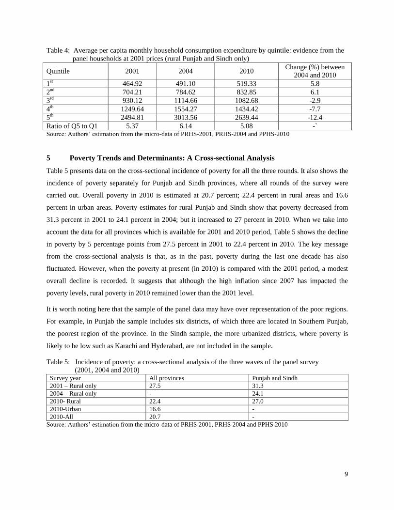
overtime (Table 3). Table 4 presents data on average per capita monthly household expenditure by

quintile for the three waves of the panel households (excluding split households) at 2001 prices. The

results are interesting. Between 2001 and 2004 period, when poverty declined markedly in rural as well as

urban areas, per capita household consumption expenditures increased for all quintiles. However, between

the 2004 and 2010 period, real expenditures increased for the bottom two quintiles while the 3rd

, 4th and

5th quintiles observed a decline in their real expenditures. This decline is modest for the 3

rd quintile, at

about 3 percent, however for the 4th and 5

th quintile, particularly for the latter, the decline in real

expenditures is substantial at around 12 percent (Table 4). It appears that the recent high inflation has an

impact on the well-being of households, particularly the top three quintiles, who have been pushed to

reduce their real expenditures.

Table 3: Socio-economic characteristics of the sampled households in 2001, 2004 and 2010

Characteristics

A cross-sectional analysis Panel Households (rural

Punjab/ Sindh only)

2001 2004 2010 2001 2004 2010

Rural Rural Rural Urban Overall

Average household size 8.0 7.7 7.8 7.0 7.6 7.9 7.9 8.1

Female headed households (%) 2.5 2.2 4.1 4.3 4.2 2.4 2.3 4.8

Mean age of head (years) 47.2 47.5 48.5 46.8 48.0 47.2 48.6 51.3

Educational attainment of the Head of Household (%)

0-5 year 80.0 83.0 76.0 61.0 71.0 80.7 80.3 78.0

6-10 year 16.0 13.0 18.0 25.0 20.0 15.5 15.2 17.0

11 and above year 4.0 4.0 6.0 15.0 9.0 3.8 4.5 5.0

All 100 100 100 100 100 100 100 100

Land ownership (%) by category

Landless households 49.1 57.5 56.6 91.2 67.4 48.1 48.8 48.2

Small landholder (upto 3 acres) 22.7 17.9 19.1 3.0 14.1 20.4 21.3 24.2

Medium landholder (> 3 to 10) 17.4 15.1 14.0 3.3 10.7 19.0 18.5 15.8

Large landholder (> 10 acres) 10.8 9.6 10.3 2.5 7.8 12.5 11.4 11.9

All 100 100 100 100 100 100 100 100

Housing Unit Ownership (%) 94.4 - 94.3 83.1 90.8 97.2 - 95.4

Livestock ownership (%) 72.2 73.6 67.1 16.1 51.2 73.9 75.6 72.6

Large animal ownership (%) 59.2 59.5 55.6 10.9 41.6 40.2 61.8 61.7

Small animal ownership (%) 42.9 50.4 43.6 9.7 33.0 65.7 51.8 49.1

House structure (%) by category

Kaccha 61.8 - 47.1 16.8 37.6 57.2 - 48.1

Mix 21.5 - 27.6 22.1 25.9 27.0 - 21.7

Pacca 16.7 - 25.3 61.1 36.5 15.8 - 30.3

All 100 100 100 100 100 100 100 100

Number of persons per room 3.9 - 4.0 3.7 3.9 4.4 - 4.3 Source: Authors‟ estimation from the micro-data of PRHS-2001, PRHS-2004 and PPHS-2010

9

Table 4: Average per capita monthly household consumption expenditure by quintile: evidence from the

panel households at 2001 prices (rural Punjab and Sindh only)

Quintile 2001 2004 2010 Change (%) between

2004 and 2010

1st 464.92 491.10 519.33 5.8

2nd

704.21 784.62 832.85 6.1

3rd

930.12 1114.66 1082.68 -2.9

4th 1249.64 1554.27 1434.42 -7.7

5th 2494.81 3013.56 2639.44 -12.4

Ratio of Q5 to Q1 5.37 6.14 5.08 -` Source: Authors‟ estimation from the micro-data of PRHS-2001, PRHS-2004 and PPHS-2010

5 Poverty Trends and Determinants: A Cross-sectional Analysis

Table 5 presents data on the cross-sectional incidence of poverty for all the three rounds. It also shows the

incidence of poverty separately for Punjab and Sindh provinces, where all rounds of the survey were

carried out. Overall poverty in 2010 is estimated at 20.7 percent; 22.4 percent in rural areas and 16.6

percent in urban areas. Poverty estimates for rural Punjab and Sindh show that poverty decreased from

31.3 percent in 2001 to 24.1 percent in 2004; but it increased to 27 percent in 2010. When we take into

account the data for all provinces which is available for 2001 and 2010 period, Table 5 shows the decline

in poverty by 5 percentage points from 27.5 percent in 2001 to 22.4 percent in 2010. The key message

from the cross-sectional analysis is that, as in the past, poverty during the last one decade has also

fluctuated. However, when the poverty at present (in 2010) is compared with the 2001 period, a modest

overall decline is recorded. It suggests that although the high inflation since 2007 has impacted the

poverty levels, rural poverty in 2010 remained lower than the 2001 level.

It is worth noting here that the sample of the panel data may have over representation of the poor regions.

For example, in Punjab the sample includes six districts, of which three are located in Southern Punjab,

the poorest region of the province. In the Sindh sample, the more urbanized districts, where poverty is

likely to be low such as Karachi and Hyderabad, are not included in the sample.

Table 5: Incidence of poverty: a cross-sectional analysis of the three waves of the panel survey

(2001, 2004 and 2010) Survey year All provinces Punjab and Sindh

2001 – Rural only 27.5 31.3

2004 – Rural only - 24.1

2010- Rural 22.4 27.0

2010-Urban 16.6 -

2010-All 20.7 -

Source: Authors‟ estimation from the micro-data of PRHS 2001, PRHS 2004 and PPHS 2010

10

Table 6 shows poverty trends in rural Punjab and Sindh for the panel households only. In panel A of the

Table, split households are excluded but the original households from which households have separated

are included. In panel B, the latter have also been excluded, leaving only pure panel households without

any split. This type of classification is likely to capture the effect of demographic change (splitting) on the

well-being of households.5 Trends are same; poverty which was 29.5 percent in 2001 declined to 23.6

percent in 2004, but it increased to 26.6 percent in 2010 (panel A in Table 6). However, the fluctuation is

more pronounced when poverty estimates are based on pure panel households (Panel B). Poverty in rural

Punjab and Sindh declined sharply from 29.5 percent in 2001 to 21.8 percent in 2004, and then it jumped

to 28 percent in 2010. The change (or decline) in poverty levels between the 2001 and 2010 period is

marginal, at only 1.5 percentage points. The other key message from panel B of Table 6 is that the

behaviour of Punjab and Sindh in change in poverty status is not similar, and even within Punjab, the

situation in Southern Punjab is markedly different from the other parts of Punjab (North/Central).

Table 6: Incidence of rural poverty in Punjab and Sindh: a cross-sectional analysis of the panel

households covered in 2001, 2004 and 2010.

Panel A 2001 2004 2010

Punjab and Sindh 29.5 23.6 26.6

Punjab 20.2 18.4 20.9

Sindh 40.2 29.2 32.6

Southern Punjab 26.2 23.4 34.1

North/central Punjab 14.6 13.8 8.2

(N) 1395 1395 1395

Panel B

Punjab and Sindh 29.5 21.8 28.0

Punjab 17.6 16.9 20.6

Sindh 42.6 27.0 35.4

Southern Punjab 25.0 22.5 35.1

North/central Punjab 11.7 12.4 8.3

(N) 1092 1092 1092 Source: Authors‟ estimation from the micro-data sets of PRHS-2001, PRHS-2004, and PPHS-2010.

Note: In panel A, same households covered in three waves are included. But, split households are excluded except

the original households from which one or more households are split. In panel B, all split households including the

original households are excluded.

In North/Central Punjab region, poverty remained almost at the same level between 2001 and 2004 (Table

6 panels A and B) while in Southern Punjab and Sindh it first declined between 2001 and 2004 and then

increased between 2004 and 2010. In Southern Punjab, the increase in poverty between 2004 and 2010 is

much larger than the decline between 2001 and 2004, thus showing a net increase in poverty between

2001 and 2010 period. Although it is difficult to explain these regional differences in poverty levels,

5 However, in this study only the differences in the incidence of poverty between different types of households are

examined. Its thorough investigation is left for the subsequent analysis.

11

however, a number of studies have shown poor physical and soft infrastructure (Arif et al., 2011), less

diversified resources with highly unequal distribution of land (Malik, 2005), poor market integration and

industrialization and fewer remittances in Southern Punjab and Sindh as compared to the North/Central

Punjab. It can also be viewed in the light of recent double-digit inflation and 2010 flood which have

disproportionately affected the poorest regions of Pakistan where the majority of households are landless

with less diversified resources. Poverty profile based on the incidence of poverty by different socio-

demographic household factors is shown in Appendix Table 2.

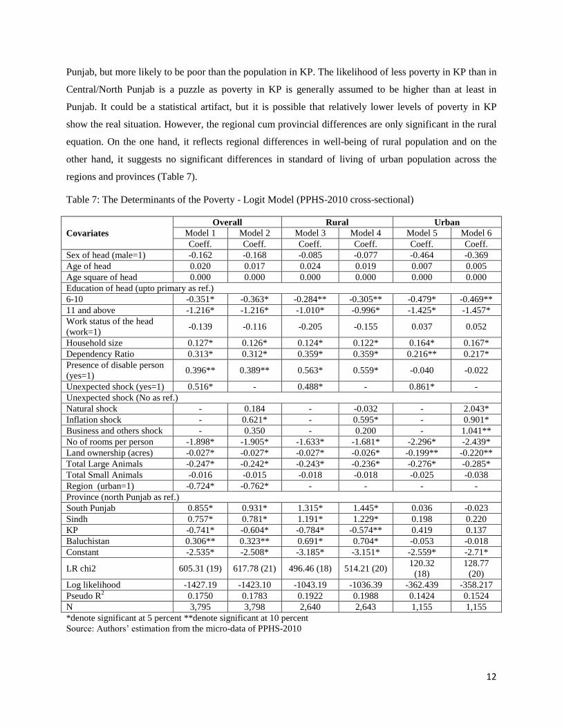
On the basis of the equation 1 (see section 3), logistic regression models have been estimated at the

national as well as rural and urban levels by using the PPHS-2010 as cross-sectional data. Three vectors

of independent variables have been included with individual characteristics of the head of the household,

household characteristics and the regional characteristics including province and region. In models 1, 3

and 5, a dummy variable of shock has been used, based on the question asked in PPHS-2010 whether the

household faced any shock during the last five years. In models 2, 4 and 6, the details of shock have been

incorporated whether the shock was natural (earthquake, drought), inflationary (inflation, food inflation)

or business (loss of job, loss in business) related.

Regarding the characteristics of the head of household, Table 7 shows that the educational attainment is

the only significant variable that has an impact on poverty reduction. Middle and higher levels of

education have a negative relation with poverty in both the rural and urban areas. Heads‟ age, sex and

work status have no significant association with poverty. The role of education in human capital,

productivity and better performance in the labour market is well documented in literature. Two

demographic factors, household size and dependency ratio, have a significant and positive relation with

poverty, suggesting that high fertility which contributes to a rise in child dependency and family size, is

likely to lower the standard of living. The presence of a disabled person in the household has a significant

and positive association with poverty overall and in rural areas. As expected, household assets, ownership

of land and livestock, have a significant and negative association with the poverty status; higher the asset

status, lower the poverty level.

Another key finding is the impact of shock on poverty. The households that faced a shock during the last

five years are more likely to be poor than households which did not face the shock. In models 2, 4 and 6,

where shocks are grouped into natural, non-natural and business categories, the impact of inflationary

shock on poverty is significant in rural areas only, while the urban poverty is prone to all the three

categories of shocks (Table 7).

However, urban population is less likely to be poor than their rural counterparts. Similarly, population of

North/Central Punjab is less likely to be poor than the populations of Sindh, Balochistan and Southern

12

Punjab, but more likely to be poor than the population in KP. The likelihood of less poverty in KP than in

Central/North Punjab is a puzzle as poverty in KP is generally assumed to be higher than at least in

Punjab. It could be a statistical artifact, but it is possible that relatively lower levels of poverty in KP

show the real situation. However, the regional cum provincial differences are only significant in the rural

equation. On the one hand, it reflects regional differences in well-being of rural population and on the

other hand, it suggests no significant differences in standard of living of urban population across the

regions and provinces (Table 7).

Table 7: The Determinants of the Poverty - Logit Model (PPHS-2010 cross-sectional)

Covariates

Overall Rural Urban

Model 1 Model 2 Model 3 Model 4 Model 5 Model 6

Coeff. Coeff. Coeff. Coeff. Coeff. Coeff.

Sex of head (male=1) -0.162 -0.168 -0.085 -0.077 -0.464 -0.369

Age of head 0.020 0.017 0.024 0.019 0.007 0.005

Age square of head 0.000 0.000 0.000 0.000 0.000 0.000

Education of head (upto primary as ref.)

6-10 -0.351* -0.363* -0.284** -0.305** -0.479* -0.469**

11 and above -1.216* -1.216* -1.010* -0.996* -1.425* -1.457*

Work status of the head

(work=1) -0.139 -0.116 -0.205 -0.155 0.037 0.052

Household size 0.127* 0.126* 0.124* 0.122* 0.164* 0.167*

Dependency Ratio 0.313* 0.312* 0.359* 0.359* 0.216** 0.217*

Presence of disable person

(yes=1) 0.396** 0.389** 0.563* 0.559* -0.040 -0.022

Unexpected shock (yes=1) 0.516* - 0.488* - 0.861* -

Unexpected shock (No as ref.)

Natural shock - 0.184 - -0.032 - 2.043*

Inflation shock - 0.621* - 0.595* - 0.901*

Business and others shock - 0.350 - 0.200 - 1.041**

No of rooms per person -1.898* -1.905* -1.633* -1.681* -2.296* -2.439*

Land ownership (acres) -0.027* -0.027* -0.027* -0.026* -0.199** -0.220**

Total Large Animals -0.247* -0.242* -0.243* -0.236* -0.276* -0.285*

Total Small Animals -0.016 -0.015 -0.018 -0.018 -0.025 -0.038

Region (urban=1) -0.724* -0.762* - - - -

Province (north Punjab as ref.)

South Punjab 0.855* 0.931* 1.315* 1.445* 0.036 -0.023

Sindh 0.757* 0.781* 1.191* 1.229* 0.198 0.220

KP -0.741* -0.604* -0.784* -0.574** 0.419 0.137

Baluchistan 0.306** 0.323** 0.691* 0.704* -0.053 -0.018

Constant -2.535* -2.508* -3.185* -3.151* -2.559* -2.71*

LR chi2 605.31 (19) 617.78 (21) 496.46 (18) 514.21 (20) 120.32

(18)

128.77

(20)

Log likelihood -1427.19 -1423.10 -1043.19 -1036.39 -362.439 -358.217

Pseudo R2 0.1750 0.1783 0.1922 0.1988 0.1424 0.1524

N 3,795 3,798 2,640 2,643 1,155 1,155

*denote significant at 5 percent **denote significant at 10 percent

Source: Authors‟ estimation from the micro-data of PPHS-2010

13

6 Analysis of Rural Poverty Dynamics

As noted earlier, only two-wave data (2001 and 2010) are available for all provinces, whereas the three-

wave data are available for Punjab and Sindh provinces. The analysis of rural poverty dynamics is carried

out in three steps. In the first step, the movement into or out of poverty are examined by the number of

waves, two or three. In the second step, a bivariate analysis for poverty dynamics has been viewed in the

context of different socio-demographic characteristics. Multivariate analyses have been carried out in the

third step. This section covers the analysis based on the first two steps, while the next section covers the

third step, the multivariate analysis. Table 8 shows results on rural poverty dynamics on the basis of two-

wave data for three periods; 2001-04; 2004-10; and 2001-10. Both the 2001-04 and 2004-10 waves

contain data for Punjab and Sindh only while the 2001-10 rounds have information for all four provinces.

Four moves of poverty, chronic poor (poor in two waves), moved out of poverty, fell into poverty and

never poor, for the provinces of Punjab and Sindh are shown in Table 8.

Table 8: Rural poverty dynamics using two-wave data

Poverty dynamics 2001-04 (Punjab

and Sindh only)

2004-10

(Punjab and

Sindh only)

2001-10 (all

provinces)

Chronic poor (poor in two waves) 9.72 8.63 9.08

Moved out of poverty 18.19 13.09 15.86

Fall into poverty 13.70 17.98 13.25

Never poor 58.39 60.30 61.82

All 100.0 100.0 100

(N) (1422) (1395) (2146) Source: Authors‟ estimation from the micro-data of PRHS-2001, PRHS-2004 and PPHS-2010

Chronic poverty (poor in two periods) was around 9 percent in all periods, whereas around 60 percent of

the population was in the `never poor‟ category, those who have not faced poverty during the two given

rounds. The remaining 30 percent of population have either moved out of poverty or fell into poverty. The

movement out of poverty out-numbered the movement into poverty in 2001-04 and 2001-10 periods. In

the 2004-10 period, however, more people fell into poverty than those who escaped poverty. Since the

chronic poverty was at the same level, around 9 percent, for all the three periods as shown in Table 8, it

appears from movement into or out of poverty data that the 2004-10 period witnessed a net increase in

poverty while it decreased during the other two periods, 2001-04 and 2001-10. In the absence of

symmetric asset distribution in rural areas of Pakistan, the overall economic growth and inflation

particularly the food inflation can suitably explain these dynamic fluctuations; during the moderate

growth period 2001-04, the net move-out of poverty took place and during the sluggish growth and

double-digit inflation particularly the food inflation (since 2007), the net movement into poverty took

place.

14

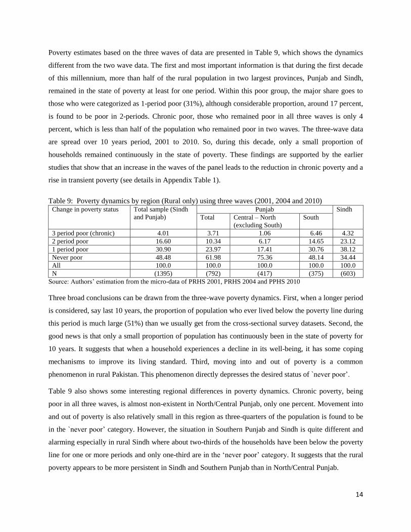
Poverty estimates based on the three waves of data are presented in Table 9, which shows the dynamics

different from the two wave data. The first and most important information is that during the first decade

of this millennium, more than half of the rural population in two largest provinces, Punjab and Sindh,

remained in the state of poverty at least for one period. Within this poor group, the major share goes to

those who were categorized as 1-period poor (31%), although considerable proportion, around 17 percent,

is found to be poor in 2-periods. Chronic poor, those who remained poor in all three waves is only 4

percent, which is less than half of the population who remained poor in two waves. The three-wave data

are spread over 10 years period, 2001 to 2010. So, during this decade, only a small proportion of

households remained continuously in the state of poverty. These findings are supported by the earlier

studies that show that an increase in the waves of the panel leads to the reduction in chronic poverty and a

rise in transient poverty (see details in Appendix Table 1).

Table 9: Poverty dynamics by region (Rural only) using three waves (2001, 2004 and 2010) Change in poverty status

Total sample (Sindh

and Punjab)

Punjab Sindh

Total Central – North

(excluding South)

South

3 period poor (chronic) 4.01 3.71 1.06 6.46 4.32

2 period poor 16.60 10.34 6.17 14.65 23.12

1 period poor 30.90 23.97 17.41 30.76 38.12

Never poor 48.48 61.98 75.36 48.14 34.44

All 100.0 100.0 100.0 100.0 100.0

N (1395) (792) (417) (375) (603)

Source: Authors‟ estimation from the micro-data of PRHS 2001, PRHS 2004 and PPHS 2010

Three broad conclusions can be drawn from the three-wave poverty dynamics. First, when a longer period

is considered, say last 10 years, the proportion of population who ever lived below the poverty line during

this period is much large (51%) than we usually get from the cross-sectional survey datasets. Second, the

good news is that only a small proportion of population has continuously been in the state of poverty for

10 years. It suggests that when a household experiences a decline in its well-being, it has some coping

mechanisms to improve its living standard. Third, moving into and out of poverty is a common

phenomenon in rural Pakistan. This phenomenon directly depresses the desired status of `never poor‟.

Table 9 also shows some interesting regional differences in poverty dynamics. Chronic poverty, being

poor in all three waves, is almost non-existent in North/Central Punjab, only one percent. Movement into

and out of poverty is also relatively small in this region as three-quarters of the population is found to be

in the `never poor‟ category. However, the situation in Southern Punjab and Sindh is quite different and

alarming especially in rural Sindh where about two-thirds of the households have been below the poverty

line for one or more periods and only one-third are in the „never poor‟ category. It suggests that the rural

poverty appears to be more persistent in Sindh and Southern Punjab than in North/Central Punjab.

15

Demographic and other characteristics of the household stratified by the number of times in poverty are

presented in Appendix Table 3. On the one hand, more female headed households are chronically poor

than the male headed households; on the other hand, the proportion of female headed households who did

not experience poverty in last 10 years (never poor) is much larger (67%) than the corresponding

proportion of male headed households (48%). It is thus difficult to jump to the conclusion that female

headed households are worse off than the male headed households.

Like in other parts of the world and consistent with earlier studies, family size and dependency ratios are

linked to poverty dynamics. Larger family size and high dependency ratios are associated positively with

chronic poverty and negatively with the desired state of „never poor‟. Movement into and out of poverty

is also more common among large households with high dependency ratio than among small households.

The persistence of poverty in terms of higher incidence of chronic poverty and lower chances of staying

in never-poor status is relatively more common among households headed by less educated persons, and

having no ownership of land and livestock, suggesting the structural nature of rural poverty in Pakistan

(Appendix Table 3).

7 Determinants of Rural Poverty Dynamics

As mentioned in section 3, the change in poverty status based on two-wave panel dataset has been

recorded in four categories: chronic poor, moved out of poverty, moved into poverty and never poor. In

the analysis of three waves, poverty dynamics have been given three categories: poor in 3-periods

(chronic), poor in 1 or 2-periods, and never poor. Determinants of rural poverty dynamics are examined

separately for two-waves and three-waves; however, the multinomial logit technique has been applied for

both types of dynamics, keeping in view the more than two categories of the dependent variable (see

section 3).

To understand better the correlates that affect rural poverty dynamics, two-wave data are used separately

for 2001-10 and 2004-10 periods. In the former, overall poverty declined while in the latter it increased.

Despite this major difference in overall poverty trends, the share of chronic poor remained unchanged,

around 9 percent, for these two periods. For the analysis of three-wave data, all the three rounds (2001,

2004 and 2010) are used. Following the poverty dynamics literature in multinomial logit models,

correlates of a base year are regressed on the poverty dynamics with four sets of independent variables.

The first set includes the characteristics of head of households (age, age2, sex and education).

Demographic and health factors are part of the second set, while economic status of households i.e. land

and livestock ownership, structure of the housing unit and room availability are entered as the third set of

independent variables. Regional and provincial dummies are used as the fourth set. All these correlates

16

are not available for all three rounds, so there is a minor variation in independent variables across the

models.

Difference in some selected independent variables between two periods has also been entered into

different models i.e. household size, dependency ratio, education of the head of household, and ownership

of land and livestock. Based on the PPHS 2010 dataset, the shock variable has also been incorporated for

2004-2010 analysis as the shock variable covers the last five years.

Six multinomial logit models have been estimated. In first four models, two-waves of panel households

have been used while in the last two models, three waves information is utilized. In these model, “non-

poor” is the reference category. Results are presented in Tables 10-12.

Take the model 1, where the correlates of rural poverty dynamics are shown for two-wave data covering

the 2001-10 period, the period when overall poverty declined (Table 10). Gender of the head of household

has no significant association with poverty dynamics. Age has turned out to be negatively associated with

movement into poverty, while age2 is positively associated with it. It suggests that an increase in the age

of head of household first empowers households through his/her economic activities not to fall into

poverty but in old age this empowerment weakens and raises the probability of households to fall into

poverty.

Education has a significant and negative association with all three poverty states, suggesting, on the one

hand, that households headed by literate persons are less likely than illiterates to be in chronic poverty or

falling into poverty. On the other hand, they are also less likely to escape poverty. It is not easy to explain

this phenomenon since education is considered as an important factor to help individuals and households

to move out of poverty. However, one possibility is that the reference category is „non-poor‟, therefore, as

compared to the non-poor, they are less likely to move out of poverty. It also indicates that while

education empowers households primarily through earnings not to fall into poverty, it is not a factor

sufficient to make a transition from poor to non-poor status.

The two demographic variables household size and dependency ratio have a positive and statistically

significant association with the chronic poverty and the probability of falling into poverty. Regarding the

movement out of poverty, dependency ratio is insignificant, but the household size has a positive and

significant sign, suggesting that it helps households to make transition out of poverty. It seems that

household size helps this transition probably when the dependency ratio is low with the addition of an

adult working member.

Economic variables including the ownership of land and livestock, housing structure (pacca) and

availability of room have a significant and negative association with chronic poverty. But these variables

17

also have a significant and negative association with the movement out of poverty. Apparently this

association is also difficult to explain. The reference category in the multinomial logit model is the `never

poor‟. So the possible explanation is that households with a better economic position in terms of land,

livestock and housing are likely to stay in the `never poor‟ status than making any transition (Table 10).

Table-10: Multinomial Logit Model: Effects of 2001 Socio-economic Characteristics on rural poverty dynamics

(2001-10)

Correlates (2001)

Model-1 Model-2

Chronic Poor

/Non-poor

Moved out

/Non-poor

Moved into

/Non-poor

Chronic Poor

/Non-poor

Moved out

/Non-poor

Moved into

/Non-poor

Sex of the head (male=1) -0.95 -0.694 0.499 -1.199** -0.813** 0.222

Age of the Head -0.03 0.031 -0.044** -0.007 0.036 -0.032

Age2 of Head 0.00 0.000 0.000** 0.000 0.000 0.000

Education of the Head -0.08* -0.038** -0.049* -0.094* -0.040** -0.084*

Household size 0.14* 0.139* 0.037** 0.218* 0.123* 0.119*

Dependency Ratio 0.24* 0.084 0.133** 0.560* 0.171 0.370*

Household with one

member abroad (yes=1) -2.69 -0.246 -0.670 -2.823 -0.203 -1.224

House Structure

(PACCA=1) -0.94* -0.443* -0.451* -0.880* -0.454* -0.467*

Electricity Connection

(yes=1) -0.56* 0.096 0.161 -0.401** 0.162 0.122

Toilet facility (yes=1) -0.62** -0.778* -0.202 -0.628** -0.766* -0.158

Animals (Nos) -0.04* -0.118* 0.002 -0.156* -0.120* -0.067*

Land Holdings (acres) -0.12* -0.034* -0.029* -0.119* -0.036* -0.041*

Number of rooms per

person -2.11* -2.295* 0.137 -3.607* -2.402* 0.099

Presence of disable person

(yes=1) 0.21 0.057 -0.404 0.222 0.047 -0.491

South Punjab/North Punjab 1.55* 0.139 1.469* 1.391* 0.218 1.501*

Sindh/North Punjab 1.94* 0.744* 1.397* 1.466* 0.814* 1.140*

KP/North Punjab -1.06** -1.147* -0.649** -1.424* -1.064* -0.853*

Baluchistan/North Punjab 1.52* 0.993* 0.865* 1.586* 1.101* 0.780*

Constant -1.81 -1.477** -2.112* -2.113** -1.436 -2.602*

Difference in Household

Size - - - 0.131* -0.031 0.139*

Difference in Dependency

Ratio - - - 0.373* 0.094 0.290*

Difference in Education of

Head - - - 0.021 -0.013 -0.074*

Difference in Land

Holdings - - - -0.016 -0.006 -0.030*

Difference in Animals - - - -0.141* 0.000 -0.085*

LR chi-2 678.13 (54) 825.30 (69)

Log likelihood -1827.00 -1706.83

Pseudo R2 0.1565 0.1947

N 2,124 2,080

*denote significant at 5 percent, **denote significant at 10 percent

Source: Authors‟ estimation from the micro-data of PRHS 2001and PPHS 2010

18

Regional dummies have some interesting features. During the 2001-10 period, population of Southern

Punjab is more likely than their counterparts in North/Central Punjab to be in the state of chronic poverty

or falling into poverty. The dummies of Sindh and Balochistan provinces are similar to Southern Punjab

except that it also has a significant and positive association with making a transition out of poverty. The

KP population, as in the cross-sectional analysis, is less likely than North/Central Punjab to be in chronic

poverty or make a transition into or out of poverty (Table 10).

In model 2, differences in the values of five correlates (household size, dependency ratio, education,

landholding and animals) between the 2001 and 2010 period are added in the multinomial logit model.

There is no major change in results compared to model 1 except that sex of the head of household which

was insignificant in Model 1 turned out to be significant in model 2. The reverse is the case for the age

(age2) of the head of households. Male headed households are less likely than households headed by

females to be in chronic poverty or to move out of poverty. However, all the new entered variables –

difference in two periods – have shown a significant and expected relation with poverty dynamics. The

difference in household size for example has a positive relation with chronic poverty or falling into

poverty. Its relation with moving out of poverty is not significant. The same is the case for the

dependency ratio. Difference in both the landholding and education has a negative and significant

association with moving into poverty. The difference in livestock ownership has also shown a negative

association with chronic poverty as well as falling into poverty (Table 10). It suggests that not only the

initial socio-demographic conditions of households but also a change in these conditions overtime has

correlation with the poverty dynamics. Thus, the message is that a positive change in socio-demographic

and economic conditions of households can lead to some positive outcomes in terms of improving the

well-being of households. Our findings are to some extent consistent with Davis (2011) who shows that

the tangible assets i.e. land, livestock are the important protective assets as compared to the less tangible

assets i.e. education and social networks. The present analysis, however, shows the importance of both

types of assets for poverty reduction.

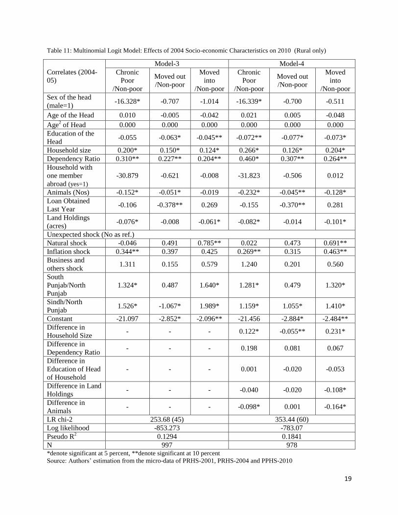
Models 3 and 4 show the multinomial logit effect for the rural poverty dynamics based on two-wave data

for the 2004-2010 period (Table 11). It is worth repeating that the 2004 round of the PRHS covered

Punjab and Sindh provinces, so the models 3 and 4 are limited to rural areas of these two provinces. But

the findings of these models are not different from the results of models 2 and 3, with couple of

exceptions. The sex of the head of household which was insignificant earlier turned out to be significant;

the male headed households are less likely than female headed households to be chronically poor. The

new variable „loan obtained last year‟ has a negatively significant association with moving out of poverty.

In other words, borrowing did not help escape poverty between the 2004 and 2010 period. Based on the

household perception data, any inflationary shock is likely to push households into poverty.

19

Table 11: Multinomial Logit Model: Effects of 2004 Socio-economic Characteristics on 2010 (Rural only)

Correlates (2004-

05)

Model-3 Model-4

Chronic

Poor

/Non-poor

Moved out

/Non-poor

Moved

into

/Non-poor

Chronic

Poor

/Non-poor

Moved out

/Non-poor

Moved

into

/Non-poor

Sex of the head

(male=1) -16.328* -0.707 -1.014 -16.339* -0.700 -0.511

Age of the Head 0.010 -0.005 -0.042 0.021 0.005 -0.048

Age2 of Head 0.000 0.000 0.000 0.000 0.000 0.000

Education of the

Head -0.055 -0.063* -0.045** -0.072** -0.077* -0.073*

Household size 0.200* 0.150* 0.124* 0.266* 0.126* 0.204*

Dependency Ratio 0.310** 0.227** 0.204** 0.460* 0.307** 0.264**

Household with

one member

abroad (yes=1)

-30.879 -0.621 -0.008 -31.823 -0.506 0.012

Animals (Nos) -0.152* -0.051* -0.019 -0.232* -0.045** -0.128*

Loan Obtained

Last Year -0.106 -0.378** 0.269 -0.155 -0.370** 0.281

Land Holdings

(acres) -0.076* -0.008 -0.061* -0.082* -0.014 -0.101*

Unexpected shock (No as ref.)

Natural shock -0.046 0.491 0.785** 0.022 0.473 0.691**

Inflation shock 0.344** 0.397 0.425 0.269** 0.315 0.463**

Business and

others shock 1.311 0.155 0.579 1.240 0.201 0.560

South

Punjab/North

Punjab

1.324* 0.487 1.640* 1.281* 0.479 1.320*

Sindh/North

Punjab 1.526* -1.067* 1.989* 1.159* 1.055* 1.410*

Constant -21.097 -2.852* -2.096** -21.456 -2.884* -2.484**

Difference in

Household Size - - - 0.122* -0.055** 0.231*

Difference in

Dependency Ratio - - - 0.198 0.081 0.067

Difference in

Education of Head

of Household

- - - 0.001 -0.020 -0.053

Difference in Land

Holdings - - - -0.040 -0.020 -0.108*

Difference in

Animals - - - -0.098* 0.001 -0.164*

LR chi-2 253.68 (45) 353.44 (60)

Log likelihood -853.273 -783.07

Pseudo R2 0.1294 0.1841

N 997 978 *denote significant at 5 percent, **denote significant at 10 percent

Source: Authors‟ estimation from the micro-data of PRHS-2001, PRHS-2004 and PPHS-2010

20

Similarly, the households who have faced the inflationary or natural shock during the last five years are

more likely than households who did not face it to be chronically poor or fall into poverty. These results

are consistent to the earlier studies6. In addition to recent inflation, the 2010 flood can also be viewed as a

major cause to push households into poverty.

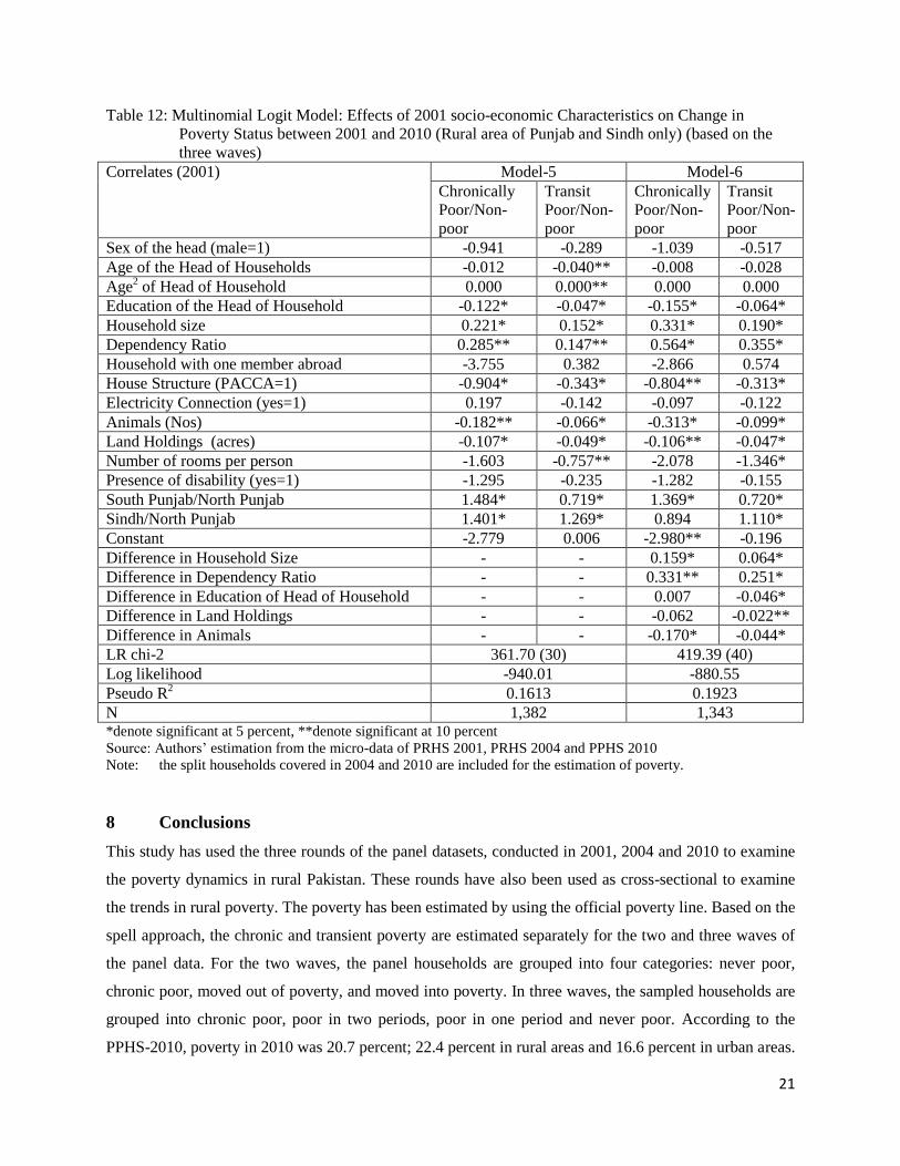
Table 12 presents the results of models 5 and 6 which are based on three-wave panel data, where the

dependent variable has three categories; chronic poor (poor in 3-periods), poor in one or two periods and

never poor. The latter is used as the reference category. The correlates are from the 2001 round of PRHS,

and the difference in selected variables between the two periods has also been added in model 6. The

findings are more consistent than the analysis based on two-wave data. For example, education of the

head of households has significant and negative relation with chronic poverty or being poor in one or two

rounds. Household size and dependency ratios have positive association with the chronic poverty as well

as being poor in one or two periods. All economic variables such as ownership of land and livestock,

structure of housing units (pacca) and availability of rooms have significant and negative association with

the chronic poverty or being poor in one or two periods. In terms of regions, both rural Sindh and

Southern Punjab are more likely than North/Central Punjab to be in the state of chronic poverty or to be

poor for one or two periods. The entry of five variables showing difference between 2001 and 2010

period does not affect the overall results (model 6). These variables also have significant association with

the poverty dynamics; an increase in household size or dependency ratio worsens the household well-

being while a positive change in household assets (land and livestock) improves it.

6 Jalan and Ravallion (2001), Sen, (2003), Davis (2011), Lawrence (2011)

21

Table 12: Multinomial Logit Model: Effects of 2001 socio-economic Characteristics on Change in

Poverty Status between 2001 and 2010 (Rural area of Punjab and Sindh only) (based on the

three waves)

Correlates (2001) Model-5 Model-6

Chronically

Poor/Non-

poor

Transit

Poor/Non-

poor

Chronically

Poor/Non-

poor

Transit

Poor/Non-

poor

Sex of the head (male=1) -0.941 -0.289 -1.039 -0.517

Age of the Head of Households -0.012 -0.040** -0.008 -0.028

Age2 of Head of Household 0.000 0.000** 0.000 0.000

Education of the Head of Household -0.122* -0.047* -0.155* -0.064*

Household size 0.221* 0.152* 0.331* 0.190*

Dependency Ratio 0.285** 0.147** 0.564* 0.355*

Household with one member abroad -3.755 0.382 -2.866 0.574

House Structure (PACCA=1) -0.904* -0.343* -0.804** -0.313*

Electricity Connection (yes=1) 0.197 -0.142 -0.097 -0.122

Animals (Nos) -0.182** -0.066* -0.313* -0.099*

Land Holdings (acres) -0.107* -0.049* -0.106** -0.047*

Number of rooms per person -1.603 -0.757** -2.078 -1.346*

Presence of disability (yes=1) -1.295 -0.235 -1.282 -0.155

South Punjab/North Punjab 1.484* 0.719* 1.369* 0.720*

Sindh/North Punjab 1.401* 1.269* 0.894 1.110*

Constant -2.779 0.006 -2.980** -0.196

Difference in Household Size - - 0.159* 0.064*

Difference in Dependency Ratio - - 0.331** 0.251*

Difference in Education of Head of Household - - 0.007 -0.046*

Difference in Land Holdings - - -0.062 -0.022**

Difference in Animals - - -0.170* -0.044*

LR chi-2 361.70 (30) 419.39 (40)

Log likelihood -940.01 -880.55

Pseudo R2 0.1613 0.1923

N 1,382 1,343 *denote significant at 5 percent, **denote significant at 10 percent

Source: Authors‟ estimation from the micro-data of PRHS 2001, PRHS 2004 and PPHS 2010

Note: the split households covered in 2004 and 2010 are included for the estimation of poverty.

8 Conclusions

This study has used the three rounds of the panel datasets, conducted in 2001, 2004 and 2010 to examine

the poverty dynamics in rural Pakistan. These rounds have also been used as cross-sectional to examine

the trends in rural poverty. The poverty has been estimated by using the official poverty line. Based on the

spell approach, the chronic and transient poverty are estimated separately for the two and three waves of

the panel data. For the two waves, the panel households are grouped into four categories: never poor,

chronic poor, moved out of poverty, and moved into poverty. In three waves, the sampled households are

grouped into chronic poor, poor in two periods, poor in one period and never poor. According to the

PPHS-2010, poverty in 2010 was 20.7 percent; 22.4 percent in rural areas and 16.6 percent in urban areas.

22

The three cross-sectional waves show fluctuations in poverty; a decline in poverty in 2001-04 period and

a rise in 2004-2010 period.

Based on the two wave panel, the analysis reveals that around 9 percent of the households were

chronically poor. It declines to only 4 percent when three-wave data is taken into account. Poverty

movements based on the three waves of panel dataset show that more than half of the rural population in

Punjab and Sindh remained in poverty for at least one period; 31 percent were categorized as 1-period

poor and around 17 percent were poor in 2-periods. In rural Sindh, about two-third of the population have

experienced at least one episode of poverty during the last 10 years.

The findings of the multivariate analysis show that demographic variables, household size and

dependency ratio have a significant positive association with chronic poverty as well as falling into

poverty. Economic variables such as the ownership of land and livestock, housing structure (pacca) and

availability of room have a significant and negative association with the chronic poverty. Both, the

inflationary and natural shocks are likely to keep households either in chronic poverty or push them into

the state of poverty. As expected, a change in both the demographic and economic factors at the

household level affects the poverty dynamics; the demographic burden increases the probability of falling

into poverty while a positive change in economic status improves the households‟ well-being.

The major challenge is how to sustain poverty reduction in rural areas in order to control both the chronic

and transitory poverty. The analysis carried out in this study suggests that it can be done through a multi-

sectoral approach that aims to: improve human capital as well as the employability of working age

population; create assets for the poor, with provision of microfinance being one source; lower the

dependency ratio by reducing fertility; and minimize the risks associated with shocks. Geographical

targeting, where the poor areas are targeted for some specific interventions, has been successful in many

parts of the developing world, like in China, in reducing poverty in a sustainable manner. This multi-

sectoral approach may be used by targeting the poor regions such as rural Sindh and Southern Punjab.

23

References

Abbi M. Kedir, and Andrew McKay (2003). Chronic Poverty in Urban Ethiopia: Panel Data

Evidence. Paper prepared for International Conference on „Staying Poor: Chronic Poverty

and Development Policy‟, University of Manchester, UK, 7 – 9 April 2003.

Adelman, Irma, K. Subbarao and Prem Vashishtha, (1985). Some Dynamic Aspects of Rural

Poverty in India. EPW, September, 1985: 106-116.

Arif, G. M. and Faiz Bilquees (2007). Chronic and Transitory Poverty in Pakistan: Evidence

from a Longitudinal Household Survey. Pakistan Development Review, 46 (2): 111–127.

Arif G. M., Nasir Iqbal and Shujaat Farooq (2011). The Persistence and Transition of Rural

Poverty in Pakistan, 1998-2004. PIDE Working Papers Series, 2011, no. 74.

Bhide, S. and Mehta, A.K. (2006). Correlates of Incidence and Exit from Chronic Poverty in

Rural India: Evidence from panel data. In Mehta, A.K. and Shepherd, A. (eds), Chronic

Poverty and Development Policy. New Delhi: Sage Publication.

Bloom, David E., David Caning and Jaypee Savilla (2002). The Demographic Dividend, A New

Perspective on the Economic Consequences of Population Change. Population Matters.

Carter M., (1999). Getting ahead or falling behind? The dynamics of poverty in post-apartheid

South Africa”, University of Wisconsin.

Cooper, E. (2010). Inheritance and the Intergenerational Transmission of Poverty in sub-Saharan

Africa: Policy considerations. University of Oxford, CPRC Working Paper 159. Manchester,

UK: Chronic Poverty Research Centre (CPRC).

Corta da L. and Joanita Magongo (2011). Evolution of Gender and Poverty Dynamics in

Tanzania. CPRC Working Paper 203. Manchester, UK: Chronic Poverty Research Centre

(CPRC).

Davis Peter (2011). The trappings of poverty: the Role of Assets and Liabilities in Socio-

economic Mobility in Rural Bangladesh. Chronic Poverty Research Centre, CPRC Working

paper, 195.

Dercan, Stefan, and Pramila Krishnan (2000). Vulnerability, Seasonality and Poverty in Ethiopia.

Journal of Development Studies, 36: (6), 82-100.

Deshingkar Priya (2010). Migration, Remote Rural Areas and Chronic Poverty in India. CPRC

Working Paper 163.

Gaiha Raghav, (1989), Are the Chronically Poor also the Poorest in India. Development and

Change, Vol. 20.

Gaiha, R. and A.B. Deolaiker (1993). Persistent, Expected and Innate Poverty: Estimates for

Semi Arid Rural South India. Cambridge Journal of Economics, 17 (4): 409-21.

Grootaert, Christiaan, Ravi Kanbur (1997). The Dynamics of Welfare Gains and Losses: An

Africa Case Study. Journal of Development Studies, 33 (5): 635- 57

Hirashima, S. (2009). Growth-Poverty Linkage and Income-Asset Relation in Regional

Disparity: Evidence from Pakistan and India. The Pakistan Development Review 48: 4 Part

1: 357-386.

24

Hoddinott, John, Trudy Owens and Bill Kinsey (1998). Relief Aid and Development Assistance

in Zimbabwe. Report to United States Agency for International Development, Washington

D.C.

Hossain M. and Abdul Bayes (2010). Rural Economy and Livelihoods, Insight From

Bangladesh. AH Development Publishing House, Dhaka.

Jalan, J. and Martin Ravallion (1999). Do Transient and Chronic Poverty in Rural China Share

Common Causes?. Paper presented as IDS/IFPRI Workshop on Poverty Dynamics, IDS,

April 1999.

Jalan, J. and M. Ravallion (2000). Is transient poverty different? Evidence for Rural China.

Journal of Development Studies, Vol. 36 (6): 82-99.

Jalan, J. and M. Ravallion (2001) Household Income Dynamics in Rural China, Policy Research

Working Paper Series 2706. The World Bank.

Jayaraman, Anuja and Jill L. Findeis (2005). Disaster, Population and Poverty Dynamics Among

Bangladesh Household. Annual Meeting of the Population Association of America.

John A. Okidi, Andrew McKay (2003). Poverty Dynamics in Uganda: 1992 to 2000. CPRC

Working Paper No 27.

Krishna Anirudh (2011). Characteristics and patterns of intergenerational poverty traps and

escapes in rural north India. CPRC Working Paper No 189.

Kurosaki, T. (2006). The Measurement of Transient Poverty: Theory and Application to

Pakistan. Journal of Economic Inequality, 4: 325–345.

Lawrence Bategeka (2011). Public Expenditure for Uganda from a Chronic Poverty Perspective.

Chronic Poverty Research Centre, Working Paper number 222.

Lohano H. R. (2009). Poverty dynamics in rural Sindh, Pakistan. Chronic Poverty Research

Centre, Working Paper number 157.

McCulloch, Neil and Bob Baulch (1999). Distinguishing the Chronically From the Transitory

Poor-Evidence from Pakistan. Working Paper No. 97, Institute of Development Studies,

University of Sussex.

Miller Robert, Francis Z. Karin….Mary Mathenge (2011). Family Histories and Rural

Inheritance in Kenya. Chronic Poverty Research Centre, Working Paper No. 220.

Orbeta Jr. Aniceto (2005). Poverty, Vulnerability and Family Size: Evidence from the Philipines.

ADB Institute Discussion Paper no. 29.

Scott, C. (2000). Mixed fortunes: A Study of Poverty Mobility Among Small Farm Households

in Chile, 1968-86” in Baulch B., Hoddinott J. (eds.) (2000): Economic mobility and poverty

dynamics in developing countries. Frank Cass Publishers: 25-53.

Sen, B., (2003). Drivers and Escape and Descent: Changing Household Fortunes in Rural

Bangladesh. World Development, 31(3): 513-534.

Singh, R.P. and Binswanger, Hans (1993). Income growth in poor dry land areas of India‟s semi-

arid tropics. Indian Journal of Agricultural Economics, Vol.48, No.1, Jan-March. Sridhar V.,

Statistics, Frontline, November 24, 2001.

Ssewanyana, Sarah N. (2009). Chronic Poverty and Household Dynamics in Uganda. Chronic

Poverty Research Centre, Working Paper No. 139.

25

Widyanti W., A. Suryahadi, S. Sumarto and A.Yumna (2009). The relationship between chronic

poverty and household dynamics: evidence from Indonesia. CPRC Working Paper no. 32.

Wlodzimierz, Okrasa (1999). Who Avoids and Who Escapes from Poverty during the

Transition? Evidence from Polish Panel Data, 1993-96. World Bank Policy Research

Working Paper 2218, November.

World Bank (2007). Pakistan Promoting Rural Growth and Poverty Reduction. Sustainable and

Development Unit South Asia Region, Report No. 39303-PK.

26

Appendix A

Logistic regression analysis is a uni/multivariate technique which allows for estimating the probability

that an event occurs or not, by predicting a binary dependent outcome from a set of independent variables.

iii XXYEp 21)|1(

)exp(1

1

)(exp1

1)|1(

21 ii

iiZX

XYEp

(1)

The equation 1 is known as the (cumulative logistic distribution function. Here Zi ranges from - to +

; Pi ranges between 0 and 1; Pi is non-linearly related to Zi thus satisfying the conditions required for a

probability model. In satisfying these requirements, an estimation problem has been created because Pi is

nonlinear not only in X but also in the ‟s, therefore OLS procedure cannot be followed. Here Pi the

probability of being poor is given by;

)exp(1

1

i

iZ

P

And 1- Pi is the probability of not being non-poor is given by;

)exp(1

11

i

iZ

P

Therefore, we can write

)exp(1

)exp(1

1 i

i

i

i

Z

Z

P

P

(2)

Pi /( 1-Pi) is the odds ratio in favor of being treated i.e. the ratio of the probability that a

household will be poor to the probability that it will be non-poor. Taking the natural log of equation 2 will

give us;

iiiii XZPPL 21)1/(ln

That is the log of the odds ratio is not only linear in X, but also linear in the parameters. L is called the

Logit. Multinomial logistic regression, sometimes referred to as polychotomous logistic regression, is the

extension of the logistic regression model when the outcome is recorded at more than two levels.

Consider a random variable Yi that may take one of several discrete values; in index 1, 2, 3….J. In this

study, dynamics of poverty is measured at 3 and 4 levels. The response variable captures the status of

household either chronic poor or transient poor, then;

)Pr( jYiij (3)

denotes the probability that the ith response falls in the jth category. For example πi1 is the probability

that ith household is „chronic poor‟. By assuming that the response categories are mutually exclusive, let

ŋi denotes the number of cases in the ith group and Yij denotes the number of responses from the ith group

that fall in the jth category, with observed value yij, then ijyJ

1ji with parameters

),...,( 21 iJiii . The probability distribution of the counts Yij given the total ŋi is given by the

multinomial distribution.

yiJ

iJ

y

i

ni

YyiJiJii

i

iJi

yYyY .....),.....Pr( 1

1

1,.....

11

(4)

27

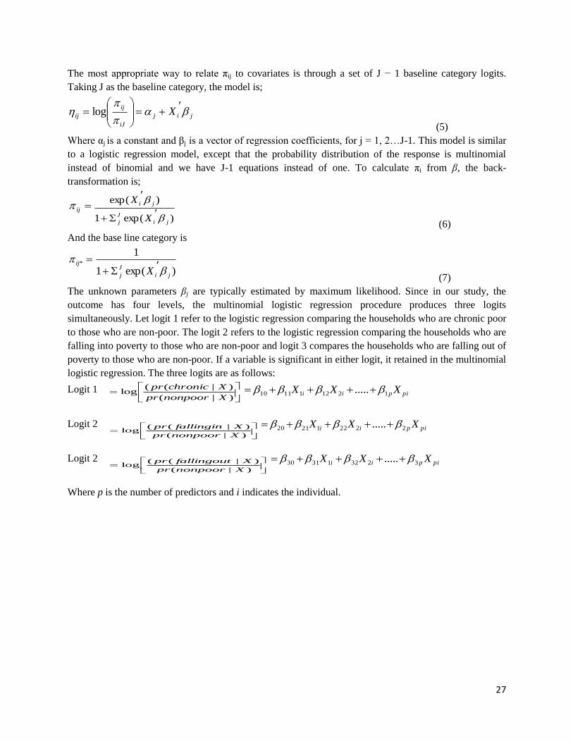
The most appropriate way to relate πij to covariates is through a set of J − 1 baseline category logits.

Taking J as the baseline category, the model is;

jij

iJ

ij

ij X

log

(5)

Where αj is a constant and βj is a vector of regression coefficients, for j = 1, 2…J-1. This model is similar

to a logistic regression model, except that the probability distribution of the response is multinomial

instead of binomial and we have J-1 equations instead of one. To calculate πi from β, the back-

transformation is;

ij)exp(1

)exp(

ji

J

j

ji

X

X

(6)

And the base line category is

*ij)exp(1

1

ji

J

j X

(7)

The unknown parameters βj are typically estimated by maximum likelihood. Since in our study, the

outcome has four levels, the multinomial logistic regression procedure produces three logits

simultaneously. Let logit 1 refer to the logistic regression comparing the households who are chronic poor

to those who are non-poor. The logit 2 refers to the logistic regression comparing the households who are

falling into poverty to those who are non-poor and logit 3 compares the households who are falling out of

poverty to those who are non-poor. If a variable is significant in either logit, it retained in the multinomial

logistic regression. The three logits are as follows:

Logit 1

)|(

)|((log

Xnonpoorpr

Xchronicprpipii XXX 121211110 .....

Logit 2

)|(

)|((log

Xnonpoorpr

Xfallinginpr pipii XXX 222212120 .....

Logit 2

)|(

)|((log

Xnonpoorpr

Xfallingoutpr pipii XXX 323213130 .....

Where p is the number of predictors and i indicates the individual.

28

Appendix Table 1: Number of waves and dynamics of poverty in different parts of the world

Country Time Frame Number

of waves Source

Welfare

Measure

% of households

Always

Poor

Someti

me Poor

Never

Poor

Chile (eight

rural

communities)

1968- 1986 2 Scott, 2000 Income per

capita 54.1 31.5 14.4

Pakistan

(IFPRI) 1988-2005 2 Lohano, 2009

Income per

capita 41.3 43.1 15.6

South Africa 1993-1998 2 Carter, 1999 Expenditures

per capita 22.7 31.5 45.8

Ethiopia 1994-1995 2

Dercon and

Krishnan,

2000

Expenditures

per capita 24.8 30.1 45.1

Pakistan

(PSES) 1998-2000 2

Arif and Faiz,

2007

Expenditure

per capita 22.4 28.8 48.8

Pakistan

(PRHS) 2001-2004 2

Arif et al.,

2011

Expenditure

per capita 11.3 32.2 56.5

Uganda 1992-1999 2 Ssewanyana,

2009

expenditure

per adult 18.4 44.5 37.1

Ethiopia 1994-95,

1997 3

Abbi, and

Andrew, 2003

expenditure

per adult 21.5

16.8 (2-

periods)

19.4 (1-

period)

51.1

India

(NCAER) 1968-1971 3 Gaiha, 1989

Income per

capita 33.3 36.7 30

India

(NCAER)

1970/71-

1981/82 3

Bhide and

Mehta, 2006

Real per capita

expenditure 21.3 17.3 61.3

Indonesia 1993,1997,

2000 3

Widyanti et

al., 2009

per capita

household

expenditure

4.2 30.1 65.7

Zimbabwe 1992-1996 4 Hoddinott et

al., 1998

Income per

capita 10.6 59.6 29.8

Uganda 1992-1996 4 John and

Andrew, 2003

Expenditure

per capita 12.8 57.3 30

Pakistan

(IFPRI) 1986-1991 5

McCulloch

and Baluch,

1999

Income per

adult

equivalent

3 55.3 41.7

China (rural) 1985 -1990 6

Jalan and

Ravallion,

1999

Expenditure

per capita 6.2 47.8 46

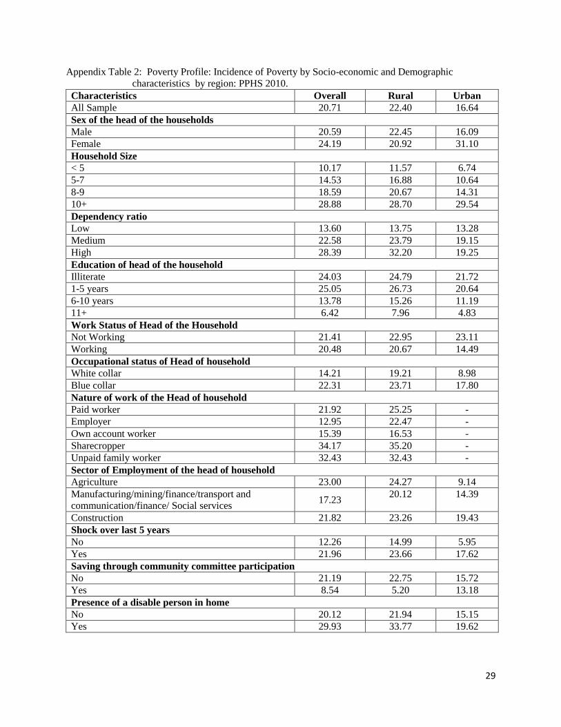
29

Appendix Table 2: Poverty Profile: Incidence of Poverty by Socio-economic and Demographic

characteristics by region: PPHS 2010.

Characteristics Overall Rural Urban

All Sample 20.71 22.40 16.64

Sex of the head of the households

Male 20.59 22.45 16.09

Female 24.19 20.92 31.10

Household Size

< 5 10.17 11.57 6.74

5-7 14.53 16.88 10.64

8-9 18.59 20.67 14.31

10+ 28.88 28.70 29.54

Dependency ratio

Low 13.60 13.75 13.28

Medium 22.58 23.79 19.15

High 28.39 32.20 19.25

Education of head of the household

Illiterate 24.03 24.79 21.72

1-5 years 25.05 26.73 20.64

6-10 years 13.78 15.26 11.19

11+ 6.42 7.96 4.83

Work Status of Head of the Household

Not Working 21.41 22.95 23.11

Working 20.48 20.67 14.49

Occupational status of Head of household

White collar 14.21 19.21 8.98

Blue collar 22.31 23.71 17.80

Nature of work of the Head of household

Paid worker 21.92 25.25 -

Employer 12.95 22.47 -

Own account worker 15.39 16.53 -

Sharecropper 34.17 35.20 -

Unpaid family worker 32.43 32.43 -

Sector of Employment of the head of household

Agriculture 23.00 24.27 9.14

Manufacturing/mining/finance/transport and

communication/finance/ Social services 17.23

20.12 14.39

Construction 21.82 23.26 19.43

Shock over last 5 years

No 12.26 14.99 5.95

Yes 21.96 23.66 17.62

Saving through community committee participation

No 21.19 22.75 15.72

Yes 8.54 5.20 13.18

Presence of a disable person in home

No 20.12 21.94 15.15

Yes 29.93 33.77 19.62

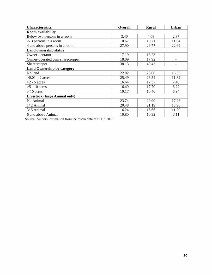
30

Characteristics Overall Rural Urban

Room availability

Below two persons in a room 3.40 4.08 2.37

2- 3 persons in a room 10.67 10.21 11.64

4 and above persons in a room 27.90 29.77 22.69

Land ownership status

Owner-operator 17.19 18.23 -

Owner-operated cum sharecropper 18.09 17.92 -

Sharecropper 38.13 40.43 -

Land Ownership by category

No land 22.02 26.00 16.33

>0.01 – 2 acres 25.49 26.54 11.82

>2 - 5 acres 16.64 17.37 7.48

>5 - 10 acres 16.49 17.70 6.22

10 acres 10.17 10.46 6.94

Livestock (large Animal only)

No Animal 23.74 29.90 17.26

1/ 2 Animal 20.48 21.19 13.98

3/ 5 Animal 16.24 16.66 11.20

6 and above Animal 10.80 10.92 8.11

Source: Authors‟ estimation from the micro-data of PPHS 2010

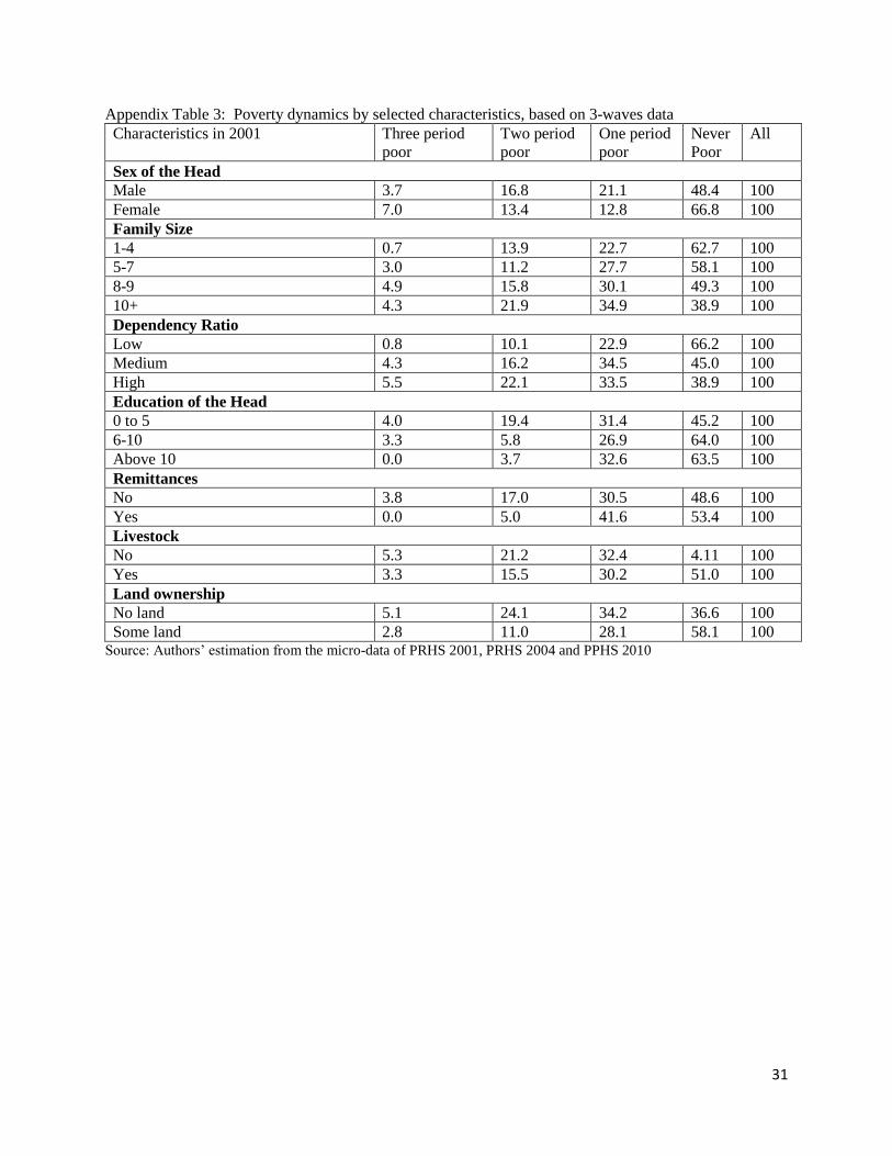
31

Appendix Table 3: Poverty dynamics by selected characteristics, based on 3-waves data

Characteristics in 2001 Three period

poor

Two period

poor

One period

poor

Never

Poor

All

Sex of the Head

Male 3.7 16.8 21.1 48.4 100

Female 7.0 13.4 12.8 66.8 100

Family Size

1-4 0.7 13.9 22.7 62.7 100

5-7 3.0 11.2 27.7 58.1 100

8-9 4.9 15.8 30.1 49.3 100

10+ 4.3 21.9 34.9 38.9 100

Dependency Ratio

Low 0.8 10.1 22.9 66.2 100

Medium 4.3 16.2 34.5 45.0 100

High 5.5 22.1 33.5 38.9 100

Education of the Head

0 to 5 4.0 19.4 31.4 45.2 100

6-10 3.3 5.8 26.9 64.0 100

Above 10 0.0 3.7 32.6 63.5 100

Remittances

No 3.8 17.0 30.5 48.6 100

Yes 0.0 5.0 41.6 53.4 100

Livestock

No 5.3 21.2 32.4 4.11 100

Yes 3.3 15.5 30.2 51.0 100

Land ownership

No land 5.1 24.1 34.2 36.6 100

Some land 2.8 11.0 28.1 58.1 100 Source: Authors‟ estimation from the micro-data of PRHS 2001, PRHS 2004 and PPHS 2010