Embed Size (px)
Citation preview

Dynamics of Quantum Correlations with Photons


Dynamics of Quantum Correlationswith Photons
Experiments on bound entanglement and contextuality for applicationin quantum information
Elias Amselem

Thesis for the degree of Doctor of Philosophy in Physicsc© Elias Amselem, Stockholm 2011c© American Physical Society (papers)c© Nature publishing group (papers)
ISBN 978-91-7447-421-3
Printed in Sweden by Universitetsservice US-AB, Stockholm, Stockholm 2011Distributor: Department of Physics, Stockholm University
Cover illustration: Foil triangles above aquarelle circles by Yohanna Amselem.

...the “paradox” is only a conflict between reality and your feelingof what reality “ought to be.”
– Richard Feynman, in The Feynman Lectures on Physics, vol III, pp. 18-9(Addison-Wesley, 1964).


Abstract
The rapidly developing interdisciplinary field of quantum information, whichmerges quantum and information science, studies non-classical aspects ofquantum systems. These studies are motivated by the promise that the non-classicality can be used to solve tasks more efficiently than classical methodswould allow. In many quantum informational studies, non-classical behaviouris attributed to the notion of entanglement.
In this thesis we use photons to experimentally investigate fundamentalquestions such as: What happens to the entanglement in a system when itis affected by noise? In our study of noisy entanglement we pursue the chal-lenging task of creating bound entanglement. Bound entangled states are cre-ated through an irreversible process that requires entanglement. Once in thebound regime, entanglement cannot be distilled out through local operationsassisted by classical communication. We show that it is possible to experi-mentally produce four-photon bound entangled states and that a violation of aBell inequality can be achieved. Moreover, we demonstrate an entanglement-unlocking protocol by relaxing the condition of local operations.
We also explore the non-classical nature of quantum mechanics inseveral single-photon experiments. In these experiments, we show theviolation of various inequalities that were derived under the assumption ofnon-contextuality. Using qutrits we construct and demonstrate the simplestpossible test that offers a discrepancy between classical and quantum theory.Furthermore, we perform an experiment in the spirit of the Kochen-Speckertheorem to illustrate the state-independence of this theorem. Here, weinvestigate whether or not measurement outcomes exhibit fully contextualcorrelations. That is, no part of the correlations can be attributed to thenon-contextual theory. Our results show that only a small part of theexperimental generated correlations are amenable to a non-contextualinterpretation.


List of Abbreviations
Symbol Description
LOCC local operations assisted by classical communication
BE bound entanglement
PT partial transpose
PPT positive partial transpose
HV hidden variable models, also referred to as classical models
EPR Einstein-Podolsky-Rosen
CHSH Clauser-Horne-Shimony-Holt
KS Kochen-Specker
H horizontal polarization
V vertical polarization
SMF single mode fibre
HWP half-wave plate
QWP quarter-wave plate
BS beam splitter, refers to a general or 50/50 BS
SPBS special polarized BS, 100/0 for H and 33/66 for V polarization
PBS polarized beam splitter
FWHM full width half maximum
PS phase shift
SPDC spontaneous parametric down conversion
APD avalanche photo diode
TTL transistor–transistor logic, 4.1V high with a 20ns duration


Contents
Abstract . . . . . . . . . . . . . . . . . . . . . . . . . . . . . . . . . . . . . . . . . . . . . . . . iList of Abbreviations . . . . . . . . . . . . . . . . . . . . . . . . . . . . . . . . . . . . . . . iiiSammanfattning på svenska . . . . . . . . . . . . . . . . . . . . . . . . . . . . . . . . viiList of Accompanying Papers . . . . . . . . . . . . . . . . . . . . . . . . . . . . . . . . ixPreface . . . . . . . . . . . . . . . . . . . . . . . . . . . . . . . . . . . . . . . . . . . . . . . . xi
My Contributions to the Accompanying Papers . . . . . . . . . . . . . . . . . . . . . . . . . xivAcknowledgements . . . . . . . . . . . . . . . . . . . . . . . . . . . . . . . . . . . . . . . . . . . . xv
Part I: Background Material and Results1 Quantum Information Basics . . . . . . . . . . . . . . . . . . . . . . . . . . . . . . 3
1.1 Bits, Qubits and Entanglement . . . . . . . . . . . . . . . . . . . . . . . . . . . . . . . . 31.1.1 The Qubit . . . . . . . . . . . . . . . . . . . . . . . . . . . . . . . . . . . . . . . . . . . 41.1.2 Multi-Qubit . . . . . . . . . . . . . . . . . . . . . . . . . . . . . . . . . . . . . . . . . . 51.1.3 Mixed States . . . . . . . . . . . . . . . . . . . . . . . . . . . . . . . . . . . . . . . . . 61.1.4 No-cloning and LOCC . . . . . . . . . . . . . . . . . . . . . . . . . . . . . . . . . . 81.1.5 Entanglement in Pure States . . . . . . . . . . . . . . . . . . . . . . . . . . . . . . 91.1.6 Entanglement in Mixed States . . . . . . . . . . . . . . . . . . . . . . . . . . . . . 111.1.7 Distillation and Bound Entanglement . . . . . . . . . . . . . . . . . . . . . . . . 12
1.2 State and Entanglement Verification . . . . . . . . . . . . . . . . . . . . . . . . . . . . . 131.2.1 State Fidelity . . . . . . . . . . . . . . . . . . . . . . . . . . . . . . . . . . . . . . . . . 141.2.2 Witness Method . . . . . . . . . . . . . . . . . . . . . . . . . . . . . . . . . . . . . . 141.2.3 PPT-Criterion . . . . . . . . . . . . . . . . . . . . . . . . . . . . . . . . . . . . . . . . 15
1.3 Hidden Variable Models . . . . . . . . . . . . . . . . . . . . . . . . . . . . . . . . . . . . . 171.3.1 Bell Inequality . . . . . . . . . . . . . . . . . . . . . . . . . . . . . . . . . . . . . . . . 171.3.2 Kochen-Specker . . . . . . . . . . . . . . . . . . . . . . . . . . . . . . . . . . . . . . 201.3.3 Fully Contextual Correlations . . . . . . . . . . . . . . . . . . . . . . . . . . . . . . 221.3.4 Klyachko et al. and Wright . . . . . . . . . . . . . . . . . . . . . . . . . . . . . . . 26
2 The Art of Quantum Optics and Data Analysis . . . . . . . . . . . . . . . . . 312.1 Implementation of Qubits . . . . . . . . . . . . . . . . . . . . . . . . . . . . . . . . . . . . 31
2.1.1 Photon Polarization . . . . . . . . . . . . . . . . . . . . . . . . . . . . . . . . . . . . 312.1.2 Path Encoding . . . . . . . . . . . . . . . . . . . . . . . . . . . . . . . . . . . . . . . . 32
2.2 Distribution of Photons . . . . . . . . . . . . . . . . . . . . . . . . . . . . . . . . . . . . . . 322.3 Single-qubit Gates . . . . . . . . . . . . . . . . . . . . . . . . . . . . . . . . . . . . . . . . . 33

vi
2.3.1 Wave Plates . . . . . . . . . . . . . . . . . . . . . . . . . . . . . . . . . . . . . . . . . 342.3.2 Beam Splitters . . . . . . . . . . . . . . . . . . . . . . . . . . . . . . . . . . . . . . . . 35
2.4 Linear Optical Two-Qubit Gates . . . . . . . . . . . . . . . . . . . . . . . . . . . . . . . . 372.4.1 Polarization-Path Gate and Polarization Analysis . . . . . . . . . . . . . . . . 382.4.2 Two-Photon Sign-Shift Gate . . . . . . . . . . . . . . . . . . . . . . . . . . . . . . 39
2.5 Down-Conversion . . . . . . . . . . . . . . . . . . . . . . . . . . . . . . . . . . . . . . . . . 442.5.1 Pump Laser . . . . . . . . . . . . . . . . . . . . . . . . . . . . . . . . . . . . . . . . . 442.5.2 Two-Photon SPDC . . . . . . . . . . . . . . . . . . . . . . . . . . . . . . . . . . . . . 452.5.3 Multi-Photon Product States . . . . . . . . . . . . . . . . . . . . . . . . . . . . . . 492.5.4 Creation of Mixed States . . . . . . . . . . . . . . . . . . . . . . . . . . . . . . . . . 50
2.6 Detection and Data Analysis . . . . . . . . . . . . . . . . . . . . . . . . . . . . . . . . . . 512.6.1 Detectors . . . . . . . . . . . . . . . . . . . . . . . . . . . . . . . . . . . . . . . . . . . 522.6.2 Multi-Channel Coincidence Unit . . . . . . . . . . . . . . . . . . . . . . . . . . . . 532.6.3 Detection Efficiencies . . . . . . . . . . . . . . . . . . . . . . . . . . . . . . . . . . . 542.6.4 Expectation Values . . . . . . . . . . . . . . . . . . . . . . . . . . . . . . . . . . . . 552.6.5 Quantum State Tomography . . . . . . . . . . . . . . . . . . . . . . . . . . . . . . 56
3 Experimental Bound Entanglement . . . . . . . . . . . . . . . . . . . . . . . . . 613.1 Bit-Flip and Phase-Flip Error Channel . . . . . . . . . . . . . . . . . . . . . . . . . . . 62
3.1.1 Probability Tetrahedron . . . . . . . . . . . . . . . . . . . . . . . . . . . . . . . . . . 643.1.2 Witness . . . . . . . . . . . . . . . . . . . . . . . . . . . . . . . . . . . . . . . . . . . . 653.1.3 Bell Inequality . . . . . . . . . . . . . . . . . . . . . . . . . . . . . . . . . . . . . . . . 66
3.2 The Experiment . . . . . . . . . . . . . . . . . . . . . . . . . . . . . . . . . . . . . . . . . . 703.2.1 State Characterization . . . . . . . . . . . . . . . . . . . . . . . . . . . . . . . . . . 703.2.2 Unlocking Entanglement . . . . . . . . . . . . . . . . . . . . . . . . . . . . . . . . . 74
4 Experiments on the Foundation of Quantum Mechanics . . . . . . . . . . 774.1 Kochen-Specker Inequality and Fully Contextual Correlations . . . . . . . . . . . 79
4.1.1 Results of the Experiment on the Kochen-Specker Inequality . . . . . . . . 834.1.2 Results on Fully Contextual Correlations . . . . . . . . . . . . . . . . . . . . . . 85
4.2 Klyachko et al. and Wright . . . . . . . . . . . . . . . . . . . . . . . . . . . . . . . . . . . 864.2.1 Results on Klyachko et al. and Wright . . . . . . . . . . . . . . . . . . . . . . . 91
5 Conclusions and Outlook . . . . . . . . . . . . . . . . . . . . . . . . . . . . . . . . . 93Bibliography . . . . . . . . . . . . . . . . . . . . . . . . . . . . . . . . . . . . . . . . . . . . . 97
Part II: Scientific Publications

vii
Sammanfattning på svenskaDet sägs att John Wheeler i sitt sökande efter den kvantmekaniska principendöpte om det till ”Merlin principen”. Legenden berättar om trollkarlen Merlinsom kunde ändra form om och om igen när han var förföljd. Detta är liktkvantmekanikens många tolkningar och den mystik som förknippas med den.
Det snabbt växande tvärvetenskapliga forskningsfältet kvantinformation ären sammanslagning av kvantmekanik och informationsvetenskap. Detta forsk-ningsfält försöker förstå sig på de icke-klassiska aspekterna av kvantmekani-ken. En av drivkrafterna är förhoppningen att kunna använda dessa systemför att lösa informations teoretiska problem mer effektivt än vad som är möj-ligt enligt den klassiska fysiken. Denna icke-klassiska del av kvantmekanikenbenämns oftast sammanflätning, eller entanglement på engelska.
I denna avhandling använder vi fotoner för att utföra experiment som un-dersöker grundläggande frågor som: Vad händer med sammanflätningen i ettsystem som är under bruspåverkan? I denna studie av brusets påverkan påsammanflätningen strävar vi efter att skapa bunden sammanflätning. Detta ärett exempel på en irreversibel process där sammanflätning behövs för att skapakvanttillstånden. Men när bruset har drivit tillståndet till den bundna regimenkan man inte destillera ut någon sammanflätning med hjälp av lokala opera-tioner och klassisk kommunikation mellan parterna. Detta trots att systemetfortfarande är sammanflätat. Vi visar i studien att det är möjligt att experimen-tellt framställa bundna sammanflätade kvanttillstånd med ett system beståendeav fyra fotoner. Dessutom visar vi att dessa tillstånd även kan bryta en Bellolikhet. Genom att bryta villkoret för lokala operationer visar vi även att detär möjligt att låsa upp den bundna sammanflätningen.
Vi utforskar även kvantmekanikens icke-klassiska inslag med hjälp av en-skilda fotoner genom att bryta mot ett flertal icke-kontextuella olikheter. Härvisar vi hur man kan konstruera det enklaste testet där det finns en diskre-pans mellan klassisk och kvant-fysik. Förutom denna studie utför vi ett expe-riment som är i samma anda som Kochen-Specker teoremet, syftet är att belysatillståndsoberoendet i teoremet. Dessutom undersöker vi korrelationer mellanmätutfallen som är helt icke-kontextuella. Detta innebär att teoretiskt kan ing-en del av de korrelationer som uppkommer tillskrivas den icke-kontextuelladelen av teorin.


ix
List of Accompanying Papers
This thesis is based on the following papers, which are referred to in the textby their Roman numerals.
I Experimental four-qubit bound entanglement, E. Amselem,and M. Bourennane, Nature physics 5, 748 (2009).
II Reply to ’Experimental bound entanglement?’, E. Amselem,and M. Bourennane, Nature physics 6, 827 (2010).
III Experimental multipartite entanglement through noisyQuantum Channel, E. Amselem, M. Sadiq and M. Bourennane,submitted (2011).
IV State-Independent Quantum Contextuality with SinglePhotons, E. Amselem, M. Rådmark, M. Bourennane, and A.Cabello, Phys. Rev. Lett. 103, 160405 (2009).
V Two Fundamental Experimental Tests of Non-Classicalitywith Qutrits, J. Ahrens, E. Amselem, M. Bourennane, and A.Cabello, submitted (2011).
VI Experimental fully contextual correlations, E. Amselem, L. E.Danielsen, A. J. López-Tarrida, J. R. Portillo, M. Bourennane,and A. Cabello, arXiv:1111.3743v1, submitted (2011).
Reprints were made with permission from the publishers.
Related Papers Not Included1. Proposed experiments of qutrit state-independent contextuality
and two-qutrit contextuality-based nonlocality, A. Cabello, E. Am-selem, K. Blanchfield, M. Bourennane, and I. Bengtsson, submitted (2011).


xi
Preface
It is said that John Wheeler in his search for the quantum principle renamedit the ”Merlin principle”. According to legend, the magician Merlin couldchange form again and again when pursued. Similarly, quantum mechanicscan be interpreted in many ways and is surrounded by mystery.
The study of quantum mechanics began at the end of the 19th and the begin-ning of the 20th century with the idea of quantizing the energy levels of black-body radiation. The birth of quantum mechanics required the introduction ofnew concepts that do not easily lend themselves to an intuitive understand-ing. One of these curious concepts is the superposition principle, which statesthat a non-separable system of states can be constructed, so-called entangledstates. In the early days of quantum mechanics the existence of non-separablestates was strongly criticized by the three eminent physicists Einstein, Podol-sky, and Rosen (EPR). In a publication from 1935 they opposed the idea ofthe existence of such states [1]; they believed that quantum mechanics cannotcompletely describe physical reality. This was the starting point of the so-called hidden variables debate. During the 1960s two important results werepresented that shed new light on the problem of hidden variables. First JohnBell managed to construct a test [2] that could rule out models favouring theideas shared by EPR. Then Simon Kochen and Ernst Specker proved theoreti-cally that the predictions of quantum mechanics cannot be reconciled with thebasic assumptions of the hidden variable theories [3]. They showed that forany quantum system with a dimension higher than two there is always a setof tests that will give rise to quantum mechanical predictions that are differentfrom those derived through classical logic. During the following years furtherprogress was achieved by Clauser, Horne, Shimony, and Holt, who gener-alised Bell’s results to obtain the CHSH inequality [4]. Alan Aspect’s exper-iment in 1981 was an even more important milestone. He performed the firstexperimental test of Bell’s inequality [5, 6]. His results showed a violation ofthe inequality, thereby confirming the quantum mechanical predictions. Sincethen, his experimental test has been refined, generalized, and experimentallyverified for many different scenarios. However, until today no complete Belltest has been experimentally realized. Loopholes in the experiments still allowthe results to be explained by hidden variable models.

xii
These developments gave rise to the new field of quantum computation andcommunication. Efforts were made to harness the non-classicality of quantummechanics in order to solve practical problems. Here the concept of entangle-ment began to play an important role, especially for quantum teleportation andsuperdense coding [7], which cannot be realized without it. In these experi-mental advances the fragile nature of quantum states became more and morean issue, since the distribution of entanglement to several distant parties wascrucial for communication tasks. To solve this experimental problem, a distil-lation protocol that takes several copies of a noisy entangled state as input andproduces higher quality entanglement as output was proposed by Bennet andcoworkers [8, 9]. Thanks to their result high quality entanglement can now, inprinciple, always be achieved for small and low dimensional systems. It wasbelieved that for larger systems a generalization existed and would eventuallybe found. But the Horodecki family discovered a set of states in 1998 [10] thatare entangled but not distillable. These interesting states became known asbound entangled states (BE). They illustrate an irreversible process that limitsthe usage of the entanglement in the system. Owing to their mixed structure,they are considered to be closer to separable classical states, that is, they areregarded as being less quantum than distillable entangled states. However, itwas found that BE states can maximally violate Bell type inequalities [11,12],thereby making them as much non-classical as any other entangled state. Ini-tially, BE states were not suitable for experiments, but in 2001 John Smolindiscovered a state [13] that is more suitable and even keeps it bound entangledin the presence of moderately high noise.
Regarding the Kochen-Specker theorem there are several experiments [14,15] attempting to catch the spirit of the proof, but they were incomplete. Theseexperiments utilize inequalities that are derived under the assumption of non-contextual hidden variables and a violation occurs only for specific quantumstates. But one of the most striking features of the Kochen-Specker proof isthat it does not refer to any quantum state. Only recently it was found that itis possible to convert this counterfactual logic to an experimentally testableinequality that is state-independent [16]. The theoretical toolbox for derivingthis kind of inequalities has greatly improved and has produced property spe-cific tests where there is a discrepancy between classical and quantum [17].
In this thesis, we study the experimental creation and characterization ofbound entanglement, and we also investigate several tests on non-contextualhidden variables with single photons. To understand the ideas around the ex-periments we begin by describing the basic concepts and necessary theoreticaltools in chapter 1. This chapter is not meant as a complete account but more asan introduction of the concepts. It serves as a guide for later chapters where theexperiments are presented. First, we discuss the concept of the qubit and in-
xiii
troduce entanglement both in its pure and mixed form, in section 1.1. We thenlook briefly into the idea of distillation that brings us to bound entanglement,see section 1.1.7. In section 1.2 we discuss different methods to characterizean experimentally generated state. In the following we discuss the idea of hid-den variable models and contextuality, section 1.3, where we introduce anddiscuss several inequalities that will be experimentally tested.
This theoretical section is followed by an experimental part, chapter 2,which describes the experimental toolbox. Here we introduce two encodingschemes for qubits together with ways to distribute and implement one-qubitgates, see sections 2.1 - 2.3. Our experiments also requires two-qubit gates,these are discussed in section 2.4, where we investigate how to implementboth two-qubit single-photon gates coupling between degrees of freedom andtwo-photon gates coupling between qubits encoded in separated photons. Forthe bound entanglement experiments a four-photon source that produces en-tanglement between pairs of photons is needed. Section 2.5 is dedicated to thesubject of spontaneous parametric down conversion (SPDC) and the creationof mixed states. Chapter 2 ends with introducing the toolbox for detection anddata analysis, specifically, we describe the method of maximum likelihoodquantum state tomography (QST) for the reconstruction of a density matrixfrom a set of measurement data.
All tools are combined in chapters 3 and 4 where each experiment with itsresults are presented. We end with a conclusion and outlook in chapter 5.

xiv
My Contributions to the Accompanying PapersBelow I comment on my contributions to the papers accompanying this thesis.The lab was under construction when I began my Ph.D. studies in the fall of2006. Hence, I have been involved in all aspects of building up a modernresearch lab, including purchasing and characterising optical components andother necessary instruments. Furthermore, I have developed various computerprograms for data communication, control systems for the experiments, anddata analysis.Paper I: In this experiment I made a major contributions in designing theexperiment. I performed all the experimental work and data analysis. Thepaper was written by all co-authors.Paper II: A concern of the bound entanglement experiment was raised by J.Lavoie, et al. [18]. The data analysis was performed by me and the reply waswritten by all co-authors.Paper III: The basic concept and building blocks did come from theexperiment of article I. When building the experiment I did a majorcontribution to the designing of the new set-up. The experiment was built byme and Muhamad Sadiq. I performed the entire data analysis and wrote thepaper with supervision of the co-authors.Paper IV: The cascaded schema and the measurement with repreparation ofthe state where developed and designed by me and Magnus Rådmark, withequal contributions. This holds true also for all the laboratory work, as wellas the entire data analysis. The paper was written by all co-authors.Paper V: Designing the time encoding scheme and set-up of the experimentwas performed by me and Johan Ahrens with equal contributions. All thelaboratory work, as well as the entire data analysis was preformed by both ofus. The paper was written by all co-authors.Paper VI: I designed the experiment and performed all the laboratory workwith equal contributions together with Magnus Rådmark. The entire dataanalysis was performed by me and the paper was written by all co-authors.

xv
AcknowledgementsThe work in this thesis could not have been completed without the help andsupport from many fantastic people. First of all, I would like to express mydeep and sincere gratitude to my supervisor Mohamed Bourennane for believ-ing in me and introducing me to the intriguing world of applied quantumness.Special thanks go to him for the opportunity to let me more or less freely muckabout in a brand new and very shiny laboratory. I would also like to give a veryspecial thanks to Adán Cabello who with great enthusiasm discussed and an-swered all my questions about contextuality. Thanks go to Ingemar Bengtson,Piotr Badziag, Gunnar Björk and Hoshang Heydari for discussions and col-laborations.
To all present and former members of the group THANKS for an inspir-ing and joyful atmosphere. In particular, a great deal of gratitude goes to mylab mates Magnus Rådmark, Hatim Azzouz, Johan Ahrens, Christian Kothe,Muhamad Sadiq, Alley Hameedi, Atia Amari and Hannes Hübel for makingthe dark lab hours seem to pass faster by having mind-boggling discussions.Also, big thanks to Isabelle Herbauts and Sören Holst who read through thethesis and providing many important comments. For the more social aspectsof the Ph.D life thanks Kate Blanchfield, Klas Marcks von Würtemberg, OlofLundberg, Istvan Zoltan Jenei and Thor Wikfeldt for the many adventures weendured. There are many more at Albanova that deserves my gratitude forhelping me and providing a pleasant atmosphere, to all of you thanks.
Finally, I would like to thank my family for the love and support that theyalways provide. Most of all my deepest gratitude and love goes to my lovelyMaria who is and will always be by my side!


Part I:Background Material and Results


3
1. Quantum Information Basics
Classical information is usually measured in units called bits, where bit isthe abbreviation for binary digit. Claude E. Shannon, often referred to as thefounder of information theory, first used this term in a landmark article [19],where he introduced the basic elements of communication. Today, informa-tion theory has truly revolutionized our way of living because it enabled theconstruction of immensely powerful electronic devices for the manipulationof strings of bits. Stimulated by these developments, a generalization of theterm to the quantum regime emerged, the quantum bit, or qubit in short.Through this generalization new and even more powerful methods of manip-ulating data beyond the presently used classical ones have emerged. Severaltheoretical proposals for a quantum computer have already been put forth aswell as many other more specialized protocols dealing with problems rangingfrom the factorization of large numbers to the secure communication betweendistant parties. Aside from pure application-oriented proposals, new tools forinvestigating more fundamental questions about the quantum world have beenproposed.
Below we will introduce the basic concepts of quantum information the-ory, from the qubit and entanglement to the more specialized concept of non-contextual inequalities, as well sa tools for detecting bound entanglement.Throughout this chapter many of these concepts will be illustrated with ex-amples. All the presented tools will be used experimentally in later chapters.
1.1 Bits, Qubits and EntanglementA bit can be defined through any two level system, whereby the two levels areoften denoted by the abstract binary numbers 0 or 1. Nevertheless, all infor-mation has to be encoded in a physical system, for example as an electricalpotential difference, 0 volts and 3.3 volts. This is a common encoding in dig-ital electronic circuits. Other common encoding options are pulsed light usedin optical fibre networks and free space set-ups such as for example remoteTV-controls.

4 Quantum Information Basics
1.1.1 The QubitContrary to a bit that can only encode two different states, a qubit can encodean infinite number of states. Nevertheless, the qubit is a two-level system likethe bit. The two levels of the qubit are here represented by the two orthogonalquantum states |0〉 and |1〉. These two states constitute a basis for the qubit,which is referred to as the computational basis. By the superposition principleany qubit state |ψ〉 can be represented by
|ψ〉= α|0〉+β |1〉, or in matrix form, |ψ〉=
(α
β
), (1.1)
where α and β are complex numbers satisfying the normalization condition|α|2 + |β |2 = 1. A qubit can be encoded in a physical system in many ways,for example by the spin of an electron, by two atomic energy levels, or by thepolarization of photons. We will discuss the encoding in more detail later inthe experimental chapter 2.
The normalization condition allows us to rewrite |ψ〉, disregarding a globalphase factor, into a more illustrative form,
|ψ〉= cos(θ
2 )|0〉+ sin(θ
2 ) · eiφ |1〉, (1.2)
where θ and φ range from 0 to 2π . In this form, |ψ〉 describes points onthe surface of a sphere, the Bloch sphere, see fig. (1.1). The axes x, y, and zrepresent the eigenstates of three observables known as the Pauli matrices,
σx =
(0 1
1 0
),σy =
(0 −i
i 0
), and σz =
(1 0
0 −1
). (1.3)
Each of the matrices has two eigenvalues, +1 and −1. The eigenstates of thethree observables are listed in table (1.1). We will denote the basis constructedout of the set of eigenstates of each operator as the σx, σy, or σz basis, respec-tively. The computational basis consists therefore of the eigenstates of the σz
operator. Note that orthogonal states lie opposite to each other on the Blochsphere and that the state orthogonal to |ψ〉 in (1.2) can be written as |ψ⊥〉 =sin(θ
2 )|0〉− cos(θ
2 ) · e−iφ |1〉. The corresponding observable for the states |ψ〉
and |ψ⊥〉 is σ(θ ,φ) = sin(θ)cos(φ)σx + sin(θ)sin(φ)σy + cos(θ)σz.From the relation given by (1.3) it is easy to see that σx corresponds to a bit
flip operation in the computational basis: applying a σx-operation on a qubitα|0〉+ β |1〉 will result in the state α|1〉+ β |0〉. Similarly, the operation σz
shifts the phase of the state by π , thereby multiplying the state |1〉 by minus 1.The operations described above are only valid in the computational basis. Forexample, in the σx basis these actions are reversed.

1.1 Bits, Qubits and Entanglement 5
Table 1.1: Pauli matrices and their eigenvectors and eigenvalues.
Observable Eigenvalues Eigenstates
σx ±1 |x,±1〉= 1√2(|0〉± |1〉)
σy ±1 |y,±1〉= 1√2(|0〉± i|1〉)
σz ±1 |z,+1〉= |0〉, |z,−1〉= |1〉
1.1.2 Multi-QubitThere are important single qubit protocols for quantum communication andcomputation, but expanding to multi-qubit systems brings about new oppor-tunities for more complex and richer tasks. When working with multi-qubitstates, all the two-qubit Hilbert spaces are combined to form a bigger space.This new Hilbert space H ⊗n = H1⊗·· ·⊗Hn contains all possible n multi-qubit pure states. The dimensionality of the space grows exponentially withthe amount of qubits used, for n qubits the dimensionality is 2n. For two qubitsthe computational basis consists of the four vectors,
|0〉1⊗|0〉2 = |00〉=
1
0
0
0
, |0〉1⊗|1〉2 = |01〉=
0
1
0
0
,
|1〉1⊗|0〉2 = |10〉=
0
0
1
0
, |1〉1⊗|1〉2 = |11〉=
0
0
0
1
.
(1.4)
Here, the subscripts 1 and 2 indicate the two different Hilbert spaces in thetensor product H1⊗H2. Generalizing this notation to include more qubits isstraightforward. Then the position in the Dirac bracket formalism refers to thedifferent local single qubit Hilbert spaces where each qubit lives.
At this point it should be stressed that each qubit in a multi-qubit system isnot required to be physically separable from the other qubits, like for exam-ple two atoms or two photons. We can construct several qubits by using one

6 Quantum Information Basics
Figure 1.1: The Bloch Sphere describes the set of states a qubit can take. An arbitrarystate |ψ〉 with its parametrization θ and φ is illustrated.
system with many degrees of freedom where each represents a qubit. Alterna-tively, we can regard a n = 2m level system as being an m-qubit system, eventhough no qubits can be physically identified directly. Our view of qubits istherefore more shaped through the physical restrictions on the type of opera-tions that can be applied and the possibilities of measuring the results of theseoperations.
1.1.3 Mixed StatesQuantum states are fragile and are easily disturbed by the environment. Thismechanism is called decoherence and couples the pure state to its surround-ings, thereby adding information that is not available for the participants usingonly the quantum system. This coupling transforms a pure state into a statisti-cal ensemble of pure states that can not be described by the pure-state formal-ism. In a laboratory environment it is practically impossible to create a perfectpure state, especially when transporting the states through noisy channels. Theresulting mixtures can be described mathematically by density operators. Wedefine the density operator ρ = |Q〉〈Q| for a pure state |Q〉. An ensemble of aset of pure states can now be described by a weighted sum of density opera-

1.1 Bits, Qubits and Entanglement 7
tors. Generally, a density operator can be described as,
ρ = ∑i ωiρi = ∑i ωi|Qi〉〈Qi|, where ∑i ωi = 1, (1.5)
where the weights ωi are interpreted as the probability distributions of thepure states, ρi = |Qi〉〈Qi|. A density operator can be represented in the matrixformalism, where the elements of the matrix are given by 〈m|ρ|n〉 for a givenbasis in the N-dimensional space with the indices n,m ∈ 1,2, ...,N for thebasis. The matrix representation is basis-dependent, but usually the compu-tational basis is used, which simplifies the indexing for multi-qubit systems.In the computational basis the indices are given by the decimal representationof the string of binary numbers that represents each separate qubit. A mixedquantum state ρ possesses, among others, the following properties:
• ρ is Hermitian and positive semi-definite. That is, the eigenvalues λi
of ρ are all real and greater than or equal to 0.• Normalization condition, Tr(ρ) = 1.• For pure sates ρ2 = ρ .• Tr(ρ2)≤ 1, where the equality holds only for pure states.• The expectation value 〈A〉 of an operator A is given by 〈A〉= Tr(A ·
ρ).
Here, Tr() is the trace, which is the summation over the diagonal elements ofa density operator in matrix-form.
Since we set out to investigate mixed states, it is crucial to understand den-sity operators. To gain some insight, let us investigate what happens to a singlequbit ρ , when it is affected by depolarizing noise. Suppose we begin with apure state |x,1〉= (|0〉+ |1〉)/
√2. In the matrix formalism its density operator
is given by,
ρ = |x,1〉〈x,1|= 12
(1 1
1 1
). (1.6)
The off-diagonal elements indicate that the state is in a coherent superpositionand can admit interference effects between its components if it is rotated bysome operator. If the state undergoes a depolarizing stage where it loses itsinterference properties then, depending on how strong this depolarization is,the state will be transformed into,
ρnoisy = p112+(1− p)ρ, where 0≤ p≤ 1. (1.7)
If the noise parameter is p = 0, the state is still described by the pure state|x,1〉. A measurement in the computational basis will give equal probabilityof finding |0〉 and |1〉, whereas in the σx basis only |x,1〉 will be found.

8 Quantum Information Basics
The noise can render the state ρ into a complete mixture 11/2, where theoriginal state is completely washed out. This happens when the parameter p is1. Again, a measurement in the computational basis will have equal probabil-ity of finding |0〉 and |1〉, but in the σx basis there the two outcomes |x,1〉 and|x,−1〉 will be also equally probable. This is due to the lack of interferencebetween |0〉= (|x,1〉+ |x,−1〉)/
√2 and |1〉= (|x,1〉−|x,−1〉)/
√2, which are
not in a coherent superposition. For p > 0 there will be a contribution of theincoherent part 11/2, which will washout some effects. This is always the casefor an imperfect experimentally generated quantum state.
Considering the Bloch sphere, fig. (1.1), a pure qubit state is representedon the surface of the sphere, through vectors with length 1. The set of mixedqubit states are be represented in the Bloch ball, which is the interior of thesphere. A mixed qubit state is represented by a shorter vector in the spherepointing from the origin, which represents the complete mixed state, 11/2.
1.1.4 No-cloning and LOCCWhen working with multi-qubit systems one can easily be lured to believe thatalmost any operation on the states is possible. This is of course not true. A sim-ple example, which has great impact on quantum cryptography and quantumcomputation, is the no-cloning theorem. The theorem states that it is not pos-sible to construct a copying machine that takes an arbitrary unknown state andmakes a perfect copy of it. The proof [7] considers a perfect copying machinethat takes an arbitrary input state |φ〉, which is to be copied, together with atarget state |s〉, a blank paper, and converts the target |s〉 to |φ〉. The copyingprocess is performed in the machine by a unitary operation U . This copyingoperation U can thus copy any two states,
U |φ〉⊗ |s〉 = |φ〉⊗ |φ〉,U |ψ〉⊗ |s〉 = |ψ〉⊗ |ψ〉.
(1.8)
However, since the inner product is preserved for unitary operations, these twoequations give 〈ψ|φ〉=(〈ψ|φ〉)2, which has only two solutions. Either |φ〉 and|ψ〉 are orthogonal or they are equal. Thus if the copying machine can faith-fully copy one state, then it can only faithfully copy one other state, namely theorthogonal one. This restriction is one of the cornerstones of quantum cryp-tography and allows for the detection of an eavesdropper in a communicationline [7].
The restriction described above is due to quantum mechanics itself and can-not be changed. Other restrictions can be applied more artificially to suit acertain scenario. An important set of operations in quantum communicationand quantum computation are local operations assisted by classical communi-

1.1 Bits, Qubits and Entanglement 9
cation (LOCC). The above restriction emerges naturally when quantum statesare distributed to separated parties. Each party can thus only manipulate thequbits which are locally available. Any type of manipulation is allowed, frommaking measurements on the qubits to only storing them or measuring themtogether with previously received qubits. Regardless of the operations per-formed on the qubits locally, it is supposed that the local results can be com-municated classically to the other parties. In doing so, the parties can try toconvert their quantum state to something that might be more useful for a par-ticular task. For two parties A and B sharing a state ρ ∈HA⊗HB, a generalLOCC operation [20] can be described by,
ρ → 1M
∑i Ai⊗Bi ·ρ ·A†i ⊗B†
i ,
where M =Tr(∑i Ai⊗Bi ·ρ ·A†i ⊗B†
i ) is the normalization, and the operators Ai
and Bi are the local operations of the parties A and B. Each operator can occurwith a certain probability that can either be induced by the parties involvedor by the environment that is outside the parties’ control. With LOCC it ispossible to describe transmission channels that induce errors when distributingqubits. Alternatively, LOCC can be used to the opposite effect, to clean up aset of states that are noisy in order to retrieve more pure quantum states thatcan be used for a multiparty quantum protocol.
1.1.5 Entanglement in Pure StatesIt is possible to create quantum states that consist of several qubits and areinseparable. In such a quantum system it is not possible to consider each out-come of a measured qubit to be independent from the measurement outcomesof the remaining qubits, regardless of the physical distance between the qubits.Correlations arising from these kinds of systems can be stronger than thoseachievable in classical physics. This strange phenomenon, called entangle-ment, has important consequences and is used in many quantum informationaltasks such as quantum teleportation. The definition of entanglement for purestates is,
Definition: A pure state |Q〉 over the partitions Pi, where i ∈ 1..n, is calledentangled if it cannot be represented as a product of pure states |φi〉Pi .That is, |Q〉 6= |φ1〉P1 ⊗·· ·⊗ |φn〉Pn . A state that can be represented by aproduct of pure sates over this partition is called a separable state.
For pure and mixed two-qubit systems entanglement is well characterized[21]. But as soon as more than two qubits are involved the task of characteriza-tion becomes significantly harder, because of the rapid increase in complexity

10 Quantum Information Basics
of the states. In the two-qubit case there are four well-known entangled states,the so-called Bell states. They are defined as,
|ψ±〉= 1√2(|01〉± |10〉), |φ±〉= 1√
2(|00〉± |11〉). (1.9)
These four states constitute an orthonormal basis spanning the two-qubitHilbert space. It is possible using only local operations to convert each of theBell states to any of the three others, for instance,
|ψ−〉= 11⊗ 11|ψ−〉, |ψ+〉= σz⊗ 11|ψ−〉|φ−〉= 11⊗σx|ψ−〉, |φ+〉= σz⊗σx|ψ−〉.
(1.10)
As can be seen, only the flip operation σx and the π phase shift operation σz
are needed. Note that 11⊗σy gives the same result as σz⊗σx up to a globalphase.
One might wonder what is so special and strange with these states. Let ustake a look at |ψ−〉. If we choose to measure the state in the σz basis wewould see that the measurement results from the two qubits are always op-posite, that is, if one is +1 then the other is −1 and vice versa. This is onlya normal correlation and one can argue that the particles are prepared in thisway. But if we choose to measure the state in the σx basis the same type ofcorrelation will be found in the measurement outcome. In fact, every time wemeasure these two qubits in the same basis we will obtain perfect anticorre-lations. Somehow the two qubits seem to communicate to align themselvesaccording to how they will be measured, even though the involved qubits canbe separated miles from each other with no means of communicating. Thesecorrelations are stronger than similar non-communicating parts of distributedand seemingly simple systems in everyday life.
It is worth noting that if one of the Bell states is distributed to two parties,Alice and Bob, and no classical communication is established between them,then all their measured data will indicate that they have each been given acompletely depolarized qubit state. This lack of communication that resultsin ignorance of the parties involved can be accounted for by taking the par-tial trace over of the ignored parties, ρB = TrA(|ψ(i)〉〈ψ(i)|). The partial tracereduces the two-qubit state to a one-qubit state by summing over elementsof the density operator to create a new operator, ρ
j,kB = ∑i〈i, j|ρ|k, i〉, where
i, j,k ∈ 0,1, referring to the qubit basis for each party. Performing this op-eration when Bob ignores Alice will leaves Bob’s qubit in the state ρB = 11/2which is the completely mixed state. A consequence of this is that if one ofthe parties is not willing to collaborate, the reduced state of one party will notinclude any information of the other. The parties need to collaborate to obtainany usable correlation.

1.1 Bits, Qubits and Entanglement 11
A collaboration is also needed when creating entanglement. Two parties,Alice and Bob, sharing a product state |ψ1〉A ⊗ |ψ2〉B can never create en-tanglement by LOCC. Each local operation UA and UB will affect only theirlocal qubit Hilbert space, UA⊗UB|ψ1〉A⊗|ψ2〉B = |ψ ′1〉A⊗|ψ ′2〉B, and the re-sult will still be a product state between Alice and Bob. Therefore, the par-ties need to meet and perform a joint measurement to create entanglement,or one of the parties needs to send parts of an pre-entangled state through acommunication channel. One way of creating entanglement is through a con-ditioning gate, which is similar to a control gate in electronics but operatingin the quantum regime. Suppose we begin with the product state |x,1〉|z,1〉=(|0〉|0〉+ |1〉|0〉)/
√2, then using a quantum control NOT-gate,
11+σz
2⊗ 11+
11−σz
2⊗σx =
1 0 0 0
0 1 0 0
0 0 0 1
0 0 1 0
, (1.11)
the state |x,1〉|z,1〉 is converted into |φ+〉. In the control NOT-gate one qubitis used as control and the other as target. If the control is |0〉 nothing willhappen to the target, but if it is |1〉 the target will undergo a flip realized bythe σx operator in (1.11). Note also that operating with the control not-gate onan entangled state |φ+〉 will transform it back into a product state. In this wayone can design a two-qubit measurement device that maps the Bell states toproduct states which are experimentally easier to measure, see section 2.4 foran experimental realization of the control NOT-gate.
1.1.6 Entanglement in Mixed StatesEntanglement in mixed states has a slightly different definition than entangle-ment in pure states.
Definition: A mixed state ρ is called entangled if it can not be written as asum of product states, that is,
ρ 6= ∑i ωiρi1⊗·· ·⊗ρ i
n , (1.12)
where 1 to n refers to the local Hilbert space that the i state is living in.States that satisfy the right hand side of (1.12) are called separable.
Also, we say that there is a separable cut in a state ρ ∈HA⊗HB if we canwrite ρ = ∑i ωiρ
Ai ⊗ρB
i , with ρAi and ρB
i being in HA and HB, respectively.We denote such a cut by A|B. For two parties only one cut can be present. But
12 Quantum Information Basics
in general when more parties are involved more cuts can exist. Specifically,for a separable state such as the right-hand side of (1.12) we have n−1 cuts,1|2|..|n.
To show whether a state is entangled or not is in general a difficult task.In the previous section 1.1.5 we have seen that the Bell states (1.9) constitutea basis and thus any pure separable state can be constructed by linear com-binations of (1.9). Thus entanglement can be lost by coherently combiningentangled pure states. A similar situation can occur when mixing pure entan-gled states. The equal weighted mixture of the Bell states |φ+〉 and |φ−〉 is anexample illustrating this fact. Even though it is constructed by two entangledstates, the equal mixture is separable and no entanglement is present,
12 |φ
+〉〈φ+|+ 12 |φ−〉〈φ−|= 1
2 |0〉〈0|⊗ |0〉〈0|+12 |1〉〈1|⊗ |1〉〈1|.
We observe that a separable cut is present between the qubits. The same hap-pens for an equal mixture of |ψ±〉. An equal mixture of all four Bell statesresults in the completely depolarized two-qubit state 11/4.
1.1.7 Distillation and Bound EntanglementMany quantum protocols rely on pure maximally entangled states such as theBell states. One important example is quantum teleportation. In fact, quantumteleportation is often the underlying effect for the protocols to work. Generat-ing and distributing perfect maximally entangled states between long distantparties is difficult. The surrounding environment induces decoherence andrenders the pure quantum state to a mixed state. Thus reliable teleportationcannot directly be achieved by distributing the resources through these noisychannels. To solve this dilemma one can use a distillation protocol. Distilla-tion is the ability to extract from many noisy states fewer states that are closerto one of the Bell states (1.9). Bennett and collaborators [8, 9] showed that itis possible for two parties to distil n < N purer entangled states from N noisyentangled states. With a sufficient amount of copies the two parties can comearbitrary close to one of the Bell states in (1.9).
A general distillation protocol can be described as follows. Suppose thattwo parties Alice and Bob have a large number N of pairs ρ ∈ HA ⊗HB
which are noisy but entangled. The joint N pairs are then described by ρ⊗N .By performing LOCC operations they can try to reduce ρ⊗N to a set of n two-qubit states with purer entanglement between them. As described in section1.1.4, operations of this form, omitting the normalization, can generally bedescribed by [10, 20],
ρ⊗n = ∑
iAi⊗Bi ·ρ⊗N ·A†
i ⊗B†i .

1.2 State and Entanglement Verification 13
Here ρ⊗n denotes the distilled states and A†i , B†
i are Alice’s and Bob’s opera-tions in their separate H ⊗N
A/B Hilbert space. The operations A†i and B†
i projectthe state ρ⊗N to a sub-space of (HA⊗HB)
⊗N which is non-separable. In short,the idea is to use a big Hilbert space and project down to a smaller one whereentanglement is more concentrated between the parties. It is assumed in dis-tillation protocols that only LOCC are used between all parties since they areseparated and cannot transport their qubits to another laboratory.
For a set of two-qubit states that are inseparable it has been shown [22] thatregardless of how small its amount of entanglement is it is always possibleto distil out a Bell state. One might falsely conjecture that any inseparablestate can be distilled. Surprisingly, this is not true in multi-qubit and higher-dimensional scenarios. There are states that are entangled and do not admitany distillation protocol [23]. These are the so-called bound entangled (BE)states, which are defined as,
Definition: If a state is entangled but is not distillable by LOCC it is called abound entangled state.
These are indeed curious states since they require entanglement when createdbut then the entanglement is not available for distillation. This situation hasbeen compared to thermodynamics [10], where there is free energy that canperform work and the bound energy which is unavailable to perform work.In the case of entanglement, the equivalent to work is for example reliabledata transmission through quantum teleportation. Thus two different types ofentanglement can be considered to exist in a noisy quantum system, a free anda bound type. Furthermore, BE is an example of an irreversible process sincemany BE states can be generated from a pure state affected by LOCC, butthen this process can not be reversed once the state is brought into a boundentangled regime. In chapter 3 we will discuss a set of BE states that we thenexperimentally investigate.
1.2 State and Entanglement VerificationTo experimentally generate a desired state is difficult and in the end we are leftwith something that is hopefully close to the desired theoretical state. If thestate is too complicated and a reconstruction of the full density matrix is notpossible, we are obliged to only look at certain characteristics of the state. Theverification of important characteristics such as entanglement and that theseproperties are the desired ones requires tools that can detect and quantify ordiscard different properties. Here we will introduce different methods that canverify the quality of an experimental state and characterise its entanglement

14 Quantum Information Basics
properties in different ways. The discussion of a very powerful method whichallows for the reconstruction of a complete density matrix is postponed to theexperimental part, section 2.6.5, because it requires some understanding of themeasurement process and the output format of measured data.
1.2.1 State FidelityIf the density matrix is available then a measure quantifying the distance be-tween two states is the fidelity. The fidelity between two state ρ and δ isdefined as,
F(ρ,δ ) = Tr(√√
ρ ·δ ·√ρ). (1.13)
If one of the states is a pure state the fidelity reduces toF(ρ, |φ〉〈φ |) =
√〈φ |ρ|φ〉. Thus the fidelity is related to the overlap
between the states ρ and |φ〉〈φ |, which is simply the probability to project thestate ρ onto the state |φ〉. The fidelity ranges from 1 for perfect resemblancebetween the states to 0 when no resemblance exists between the states. Noresemblance is here equivalent to orthogonality and perfect resemblancemeans that the prepared state is equal to the desired one.
1.2.2 Witness MethodTo verify if an experimental state has the proper entanglement properties onecan use a witness operator. This is a powerful technique which tests with ratherfew measurements the entanglement properties of an experimental state. Awitness operator ω is defined as an observable with negative expectation valueTr(ωρ)< 0 for a set of states ρ that has the desired entanglement properties. Apositive expectation value Tr(ωρ)≥ 0 indicates that the state might not havethe right entanglement properties but it is not conclusive. It has been shownthat for each inseparable state ρ in a bi-party system in H1⊗H2 there existsan operator ω such that Tr(ωρ) < 0 and Tr(ωρ) ≥ 0 for all separable states[24]. This would not be particularly useful if it had not also been found that awitness ω could be optimised [25,26] and decomposed by local measurements[26, 27].
Maximum Overlap WitnessFinding a witness can be a tedious task, but fortunately there are some generalresults which simplify the search. Maybe the most common witness optimiza-tion for an expected state is the maximum overlap witness [28],
ω = α · 11−|ψ〉〈ψ|. (1.14)

1.2 State and Entanglement Verification 15
Here α =max|φ〉∈ϒ(|〈ψ|φ〉|2) is the maximum overlap of |ψ〉〈ψ| calculated forall states in the set ϒ that are to be disregarded. Finding α gives an operatorthat can indicate whether a state is close to |ψ〉 and has the same entanglementproperties.
In the two-qubit case the optimization is over the set ϒ of all separablestates. For the two qubit Bell states four witnesses can be constructed, theseare given by,
ωψ± =12 · 11−|ψ
±〉〈ψ±|ωφ± =
12 · 11−|φ
±〉〈φ±|.(1.15)
The only task left is to decompose these witnesses into local measurable op-erators. In this case this is easy since the Bell states can be rewritten in a formcontaining only squares of Pauli matrices (1.3) and the identity matrix.
Stabilizer WitnessAnother method is to use stabilizers [26] to find a witness. Instead of usingthe state |ψ〉 one uses the operators that stabilizes the state. A stabilizer Si isan operator which has |ψ〉 as an eigenstate and 1 as eigenvalue, Si|ψ〉 = |ψ〉.The idea is that many N qubit entangled states are uniquely defined by N sta-bilizers which are composed of local sigma matrices. By only knowing someof the stabilizers a witness can be constructed. Furthermore, for mixed statesthis method can simplify the search by finding stabilizers that stabilize themixed state and not only some of the pure states in the mixture. An impor-tant condition for constructing a witness with stabilizers is that the stabilizerscannot commute over the set of states which is used in the optimization. Thereason for this is that two stabilizers commute if and only if there is a pureproduct state among their common eigenstates [26]. A witness can be foundby replacing the state in (1.14) by stabilizers,
ω = α · 11−∑i Si, (1.16)
where α = max|φ〉∈ϒ(〈φ |∑i Si|φ〉) is the maximum expectation value calcu-lated for all states in the set ϒ that are to be disregarded. It is not necessary tooptimize over mixed states since α will also give a bound for all mixed statesthat can be constructed from the set ϒ. This witness approach will be usedlater on to find entanglement witnesses for bound entangled states.
1.2.3 PPT-CriterionAsher Peres [21] derived a powerful and useful separability criterion called thepositive partial transpose (PPT) criterion. It states that a state ρ ∈HA⊗HB
is entangled if its partial transpose ρ tB = 11⊗ TB · ρ has a negative eigen-value. The partial transpose is defined by expanding ρ in the product basis

16 Quantum Information Basics
|ai,b j〉 ∈HA⊗HB. Each position of the elements ρi, j,k,l = 〈ai,b j|ρ|ak,bl〉 ofρ is transposed such that ρ tB elements are ρ
tBi, j,k,l = ρi,l,k, j. Partial transposition
is basis-dependent but the spectrum is not.To see how this criterion can be used let us assume we have a bipartite
separable state ρ = ∑i ωiρAi ⊗ρB
i . Taking the partial transpose means that wetranspose only one of the subsystems, say B,
ρ tB = ∑i ωiρAi ⊗ (ρB
i )t . (1.17)
Since ρ and ρBi are quantum states they have real and positive eigenvalues.
The transposition does not effect the eigenvalues, thus (ρBi )
t is a legitimatestate and also ρ tB , which means that it must have positive eigenvalues. Thisshows that one always has a positive partial transpose over any separable cut.
As a simple counter-example let us apply the PPT-criterion on the stateρφ+ = |φ+〉〈φ+|, where |φ+〉 ∈HA⊗HB is one of the Bell states in (1.9). Inthe matrix formulation expressed in the computational base we obtain,
ρφ+ =
1 0 0 1
0 0 0 0
0 0 0 0
1 0 0 1
=⇒ ρtBφ+ =
1 0 0 0
0 0 1 0
0 1 0 0
0 0 0 1
. (1.18)
The eigenvalues of ρφ+ are 0 and 1. After partial transposition of qubit B thedensity operator ρ
tBφ+ has the eigenvalues−0.5 and 0.5. As expected, we obtain
a negative eigenvalue indicating that the state is entangled.For systems of dimension 2⊗ 2 and 2⊗ 3 it is a sufficient and necessary
condition, thus giving a complete characterization of separability. In higherdimensions the criterion is no longer sufficient. The insufficiency is relatedto the fact that the PPT-criterion is not only a powerful method for detect-ing entanglement, but it is closely related to entanglement distillation [10]. Asmentioned above, separable states do not violate the PPT-criterion and are alsonon-distillable since no entanglement can be created by LOCC over a separa-ble cut. More generally it was shown that the violation of the PPT-criterion isa necessary condition for distillation [10]. But if a state violates the PPT cri-terion, then entanglement is present and there might be a distillation protocolthat can be used. Thus entangled states that do not violate PPT are not distill-able and are bound entangled by definition. It is still an open question if thereare bound entangled states which violate the PPT-criterion. A complete char-acterization of the experimental density matrix is required to experimentallyevaluate the partial transpose.

1.3 Hidden Variable Models 17
1.3 Hidden Variable ModelsRegarding measurements, quantum mechanics differs greatly from classicalphysics. In contrast to the perfect measurement outcomes predicted by classi-cal physics, only statistical predictions can be deduced by quantum mechan-ics. Nevertheless it is possible to construct correlations between measurementoutcomes which are stronger than allowed by classical physics. These differ-ences allowed Einstein, Podolsky, and Rosen (EPR) to propose a paradoxicalexample [1], which suggests that quantum mechanics only gives an incom-plete description of nature. This example started the debate on whether quan-tum mechanics can be completed with hidden variables (HV). Schrödingerpointed out the fundamental role of quantum entanglement in EPR’s exampleand concluded that entanglement is “the characteristic trait of quantum me-chanics” [29]. However, Bohr argued that similar paradoxical examples occurevery time we compare different experimental arrangements, without the needof entanglement nor composite systems [30].
The underlying idea in the HV models is to consider reasonable assump-tions of the world, for example that each particle has preestablished quanti-ties, and then investigate if quantum mechanics could be substituted by thistheory and satisfy all assumptions. John Bell constructed a hidden variablemodel [31] in 1966 that could predict all outcomes of any measurement ona two-level system like a qubit. This was followed by two proofs of the con-trary for systems with higher dimensionality than a qubit, the Kochen-Speckertheorem [3, 32] and Bell’s inequality [2].
Here we will discuss and present several inequalities that will be used lateron in the experiments. First we look at a Bell-type inequality derived byClauser-Horne-Shimony-Holt (CHSH) where each party is at separated lo-cations. This inequality will then be expanded from two to four parties for theexperiments on bound entanglement. Then three inequalities are presentedwhich are more in the spirit of Kochen-Specker. These can be tested by se-quential measurements on a single system. Each of these inequalities tries tocapture different aspects of the non-classicality of quantum mechanics andwill subsequently be subjected to experimental verification.
1.3.1 Bell InequalityEntanglement admits correlations in a system that are stronger than correla-tions in classical physics. This gives rise to quantum systems that look likethey can affect each other without any link between them. This is capturedin Einstein’s correspondence with Born where he famously derided entangle-ment as “spooky action at a distance”. To resolve this matter hidden variablemodels with desired constrains where proposed. But John Bell managed to

18 Quantum Information Basics
derive inequalities that give a bound for the correlations allowed by the hid-den variable assumptions [2] but when applied to an entangled quantum statea violation occurs. This violation indicates that no HV model that satisfies allthe assumptions can reproduce all predictions asserted by quantum mechan-ics. Besides indicating that the system at hand cannot be described by a HVmodel this also gives us a tool to verify that entanglement is present in anexperimental state.
Derivation of Clauser-Horne-Shiminy-Holt InequalityThe derivation of the Clauser-Horne-Shiminy-Holt (CHSH) inequality for twoparties proceeds as follow [4,33–35]: Let us put aside quantum mechanics forthe derivation. Suppose two parties Alice and Bob are situated in differentlaboratories. In both laboratories there is some type of equipment with twolamps on it, one indicating the value +1 and the other −1. There also is aknob that can be set in two different ways. For Alice this adjustable parameteris denoted by a and for Bob similarly by b. Let us refer to this equipment asa measurement box; we do not concern ourselves with its function or innerworkings. Both parties are monitoring the blinking lamps and are keepingrecords of the events, ±1, depending on the settings, a and b. The probabilitythat the outcome is i ∈ +1,−1 when the setting a is set on Alice’s side isP(i|a). This probability can be calculated from the records that are kept. In thesame way Bob can calculate P( j|b) from the setting b and from j ∈ +1,−1.After completion of the experiment they can together through their recordscalculate the joint probability P(i, j|a,b) of obtaining the outcome i with thesetting a on Alice’s side and j with the setting b on Bob’s side. We imposetwo crucial assumptions about locality and realism in our experiment:
• Realism: The probabilities do not need to depend solely on the pa-rameter a and b but also on some set of parameters λ . These pa-rameters characterise any other dependency that the probability of anevent can depend on but are unknown or disregarded by the parties;λ is usually referred to as the hidden variable. Let P(λ ) be the proba-bility that the parameter λ will occur. The result of Alice’s statisticalmeasurement P(i|a) is then given by ∑λ P(i|a,λ ) ·P(λ ) and similarlyfor Bob with his parameters. Any correlations between the systemscome from the parameter λ and are described by joint probabilitiesof the form P(i, j|a,b) = ∑λ P(i, j|a,b,λ ) ·P(λ ).• Locality: The probability measured on Alice’s (Bob’s) box is in-
dependent of any distant system such as Bob (Alice), it only de-pends on its local environment. This implies that the joint probabilityP(i, j|a,b,λ ) can be factorized as P(i|a,λ ) ·P( j|b,λ ). This is usually

1.3 Hidden Variable Models 19
guaranteed with a spacelike separation between the parties when theychoose the measurement settings and agree upon the definition of acoincidence.
The first assumption allows us to assume that Alice’s (Bob’s) probabilitiesare governed by her (his) choice of settings and some parameter λ . Note thatwe have not assumed that Alice (Bob) can deterministically know which out-come will happen even if she (he) knows λ , but it has been shown [36, 37]that one can always extend a hidden variable of a non-deterministic model toa deterministic one where the probabilities of the form P(i|a,λ ) are either 1 or0. Together with the second assumption the result is that the two systems arecompletely decoupled from each other aside from the classical link that theparameter λ offers. Correlations between Alice and Bob are thus describedby joint probabilities of the form P(i, j|a,b) = ∑λ P(i|a,λ )P( j|b,λ )P(λ ). Wewill refer to correlations that are built up by joint probabilities of this type asclassical correlations, and in this context they describe local-realistic models.
The expected average outcome between Alice and Bob with the settings aand b is then given by,
E(a,b) = ∑i, j i · j ·P(i, j|a,b)= ∑i, j ∑λ i · j ·P(i|a,λ )P( j|b,λ )P(λ )= ∑λ E(a,λ )E(b,λ )P(λ ).
(1.19)
Here, E(a,λ ) is for example from the local expectation value given by E(a) =∑i ∑λ i ·P(i|a,λ )P(λ ) = ∑λ E(a,λ )P(λ ), where E(a,λ ) = ∑i i ·P(i|a,λ ). Ob-serve that the functions E(a,λ ), E(b,λ ) and E(a,b) range from a perfect op-posite result −1 to a perfect equal result 1. Now let us look at the followingmeasurement sequence,
| E(a,b)+E(a,b′) |+ | E(a′,b)−E(a′,b′) |≤∑λ (| E(a,λ ) || E(b,λ )+E(b′,λ ) |+ | E(a′,λ ) || E(b,λ )−E(b′,λ ) |)P(λ )
≤∑λ (| E(b,λ )+E(b′,λ ) |+ | E(b,λ )−E(b′,λ ) |)P(λ )≤ 2 ,
where we have used | E(a,λ ) |≤ 1 and that the sum of real values is lessthen the sum of the absolute values. For the last step we used the lemma that| x+ y |+ | x− y |≤ 2 for x,y ∈ [−1,1]. Thus the inequality becomes
| E(a,b)+E(a,b′) |+ | E(a′,b)−E(a′,b′) |6 2 , (1.20)
which is the CHSH inequality. How is this related to quantum mechanics?The expected average outcome E(a,b) is defined in quantum mechanics asE(a,b) = Tr(A(a)⊗B(b) ·ρ), where A(a), B(b) are quantum operators and ρ

20 Quantum Information Basics
the state produced by a source that is distributed to the parties. Experimentally,the quantity E(a,b) is usually calculated through the formula E(a,b) = ∑i, j i ·j ·P(i, j|a,b).
To illustrate the violation of (1.20) by quantum mechanics we use the oper-ators,
A(a = x) = σx, A(a′ = z) = σz
B(b =+) = σx+σz√2, B(b′ =−) = σx−σz√
2.
(1.21)
If the source produces the pure state ρ = |ψ−〉〈ψ−|, the terms on the left-handside of (1.20) are all equal to −1/
√2 except for the last term which is equal
to 1/√
2. The sum of these numbers gives | −2√
2 | 2. This violation can beshown to be the maximum allowed by quantum mechanics [38]. Thus for anyquantum mechanical systems and irrespective of the way of measurement, onecan never obtain a value greater than 2
√2 in a bipartite scenario as described
above.In the above derivation there is no reference to what type of state and mea-
surements the inequality is supposed to be optimized in order to obtain a vio-lation. For instance violation is also obtained for |φ+〉, but not for all mixturesor superpositions between the two states |ψ−〉 and |φ+〉. In contrast, we ob-tain no violation for |ψ+〉 and |φ−〉 when using the operators in (1.21); theleft-hand side of the inequality (1.20) is then 0. But by switching b and b′ in(1.21), B(b =−) and B(b′ =+), a maximal violation is again obtained.
1.3.2 Kochen-SpeckerThe Kochen-Specker (KS) theorem illustrates with great precision Bohr’s in-tuition that each time we compare different experimental arrangements para-doxical conclusions can be drawn. The theorem states that, for every physicalsystem with dimension higher than two there is always a finite set of testssuch that it is impossible to assign them predefined non-contextual results inagreement with the predictions of quantum mechanics. Remarkably, the proofof the KS theorem requires neither a composite system nor any special quan-tum state, it holds for any physical system with more than two internal levels,independent of its state.
Here we like to assign values to a set of observables that are in a non-contextual setting. To understand what contextuality means let us first considercompatible measurements.
• Compatible measurement: If a physical system is prepared in sucha way that the result of test [experiment] A is predictable and repeat-able, and if a compatible test B is then performed (instead of test A)

1.3 Hidden Variable Models 21
a subsequent execution of test A shall yield the same result as if testB had not been performed [39].• Non-contextuality: A non-contextual model is a model where the
measurement of A does not depend on which context A is measuredin. If B and C are compatible with A but not necessarily with eachother then the two contexts, A measured together with B or A mea-sured together with C, are not changing the outcome of A.
In quantum mechanics, compatibility means that the operators A and B com-mute, that is, there is at least one basis that diagonalises both operators. Fora two-level system, two non-equal tests can never be found to be compatiblesince if two operators commute they must be the same up to a global phase,but for three and higher levels it is possible. Note also that in classical physicswe assume that any set of experiments can always be made to be compati-ble by carefully performed measurements. The proof that we will describe isbased on counterfactual logic in a four level system derived by Mermin [40].We will later restate this KS proof in form of an inequality which can be testedexperimentally.
Proof of the KS TheoremConsider the nine dichotomic observables in (1.22). Each observable can havethe value +1 or −1.
A = σz⊗ 11, B = 11⊗σz, C = σz⊗σz,
a = 11⊗σx, b = σx⊗ 11, c = σx⊗σx,
α = σz⊗σx, β = σx⊗σz, γ = σy⊗σy .
(1.22)
Let us assume that we can ascribe the values υ(A), υ(B), ...,υ(γ) to each ob-servable. It is possible to construct several constraints that need to be satisfiedby observing that each row and column of (1.22) constitutes of compatibleobservables. Due to the fact that if a functional relation F(A,B, ..) = 0 holdsfor a set of compatible observables then the results of measuring the set ofobservables must also satisfy F(υ(A),υ(B), ..) = 0, we obtain the constraints:
υ(A)υ(B)υ(C) = 1, υ(a)υ(b)υ(c) = 1, υ(α)υ(β )υ(γ) = 1,
υ(A)υ(a)υ(α) = 1, υ(B)υ(b)υ(β ) = 1, υ(C)υ(c)υ(γ) =−1 .(1.23)
All constrains need to be satisfied simultaneously for a given set of valuesυ(A), υ(B), ..., υ(γ) ascribed to the observables. Thus the product of all left-hand sides in (1.23) must give a result of 1, since each value appears twice.But now we get a contradiction with the product of the right-hand side whichis equal to −1. Thus it is not possible to fulfil all constraints in (1.23) byassuming that the operators have fixed values and are non-contextual.

22 Quantum Information Basics
State-independent KS InequalityIn contrast to a Bell inequality that is violated by certain quantum states, theKS theorem uses counterfactual logic without referring to any particular state.It was found by Cabello [16] that one can construct an inequality that capturesthe impossibility to assign values υ(A), υ(B), ...,υ(γ) to the observables in(1.22). The inequality reads,
〈χ 〉= 〈ABC 〉+ 〈abc〉+ 〈αβγ 〉+ 〈Aaα 〉+ 〈Bbβ 〉−〈Ccγ 〉 ≤ 4 , (1.24)
where the bound can be found by performing an exhaustive search over all 29
possible ways of ascribing the values ±1 to υ(A), υ(B), ..., υ(γ) . Quantummechanically, the operator product of each row or column gives the identityoperator up to a sign, ABC = abc = αβγ = Aaα = Bbβ = −Ccγ = 11. Thismeans that for each measured state the obtained expectation value of each termin (1.24) will always be 1 except for the last term which is −1, thus 〈χ 〉 = 6regardless of the state.
1.3.3 Fully Contextual CorrelationsAs already mentioned, quantum correlations can be stronger than those al-lowed by classical physics. This leaves the question of what part of a violationof an inequality can be attributed to the “classical” model. Here we identify asimple non-contextual inequality, where the quantum violation cannot be im-proved by any hypothetical post-quantum resource. This will bound the partwhich can be attributed to a “classical” model to zero. The simplicity of theinequality offers an experimental approach to give a very low bound on thecontent. This will be discussed in detail in section 4.1, where the experimentis presented.
To reveal that there are some contextual correlations in an experiment, it iscommon to violate an inequality, which is an expression like,
I(P) = ∑Ta1...anx1...xnP(a1 . . .an|x1 . . .xn)≤ΩNC ≤ΩQ ≤ΩC, (1.25)
where Ta1...anx1...xn are real valued numbers and ΩNC is the maximum valueof the left-hand side for non-contextual correlations. Similarly, ΩQ and ΩCdenote the maximum value of the left-hand side for quantum and contextualcorrelations, respectively. Also, P(a1 . . .an|x1 . . .xn) are the joint probabilitiesof obtaining outcomes a1 . . .an, when compatible measurements x1 . . .xn areperformed. The non-contextual theories are those for which we can writeP(a1 . . .an|x1 . . .xn) = ∑λ P(λ )∏
ni=1 P(ai|xi,λ ). Note that this is only a gen-
eralization of the local hidden variable models obtained during the deriva-tion of the CHSH-inequality. The difference here is that we must explic-

1.3 Hidden Variable Models 23
itly assume that the measurements x1 . . .xn are compatible. For the CHSH-derivation, compatibility is guaranteed by a spacelike separation between theparties. When a separation can be accomplished then (1.25) is a Bell inequal-ity instead.
The joint probabilities P(a1 . . .an|x1 . . .xn) for contextual models, satisfyingP(a1|x1) = ∑a2 . . .∑an P(a1a2 . . .an|x1x2 . . .xn) for all x2 . . .xn and similarly forany other P(ai|xi), can be expressed in terms of a non-contextual and a con-textual part as:
P(a1 . . .an|x1 . . .xn) = wNC ·PNC(a1 . . .an|x1 . . .xn)
+(1−wNC) ·PC(a1 . . .an|x1 . . .xn),(1.26)
where 0 ≤ wNC ≤ 1 is the fraction of non-contextual correlations and (1−wNC) is the fraction of contextual correlations. To quantify the amount at-tributed to the non-contextual part in the joint probabilities P(a1 . . .an|x1 . . .xn)we can use wNC. But the decomposition (1.26) might not be unique, thereforewe focus on the decompositions that maximizes wNC.
Definition: We call the maximum of wNC over all possible decompositions ofthe form (1.26) the non-contextual content and denote it by WNC.
Note that the decomposition (1.26) and the definition is parallel to the onesintroduced in [37, 41]. In fact, for correlations generated through spacelikeseparated experiments, the non-contextual content is exactly the local contentdefined in [41].
Any experimental violation of an inequality of the form (1.25) provides anupper bound on WNC, specifically we have the relation,
WNC ≤ΩC−Ωexp
ΩC−ΩNC. (1.27)
This follows from the fact that we can divide left-hand side of (1.25) for anyexperiment into a part containing the non-contextual correlations and into an-other part containing the contextual correlations as in (1.26),
Ωexp≡WNC ·I(PNC)+(1−WNC) ·I(PC)≤WNC ·ΩNC+(1−WNC) ·ΩC. (1.28)
If we believe in quantum mechanics then the maximal experimental violationoccurs when Ωexp = ΩQ, thus the smallest value of the numerator of (1.27)is obtained when we saturate the quantum bound. To reveal fully contextualcorrelations, WC = 0, the best option is to test a non-contextual inequality suchthat it is violated by quantum mechanics and its maximum quantum valueequals its maximum contextual value, ΩNC < ΩQ = ΩC.
24 Quantum Information Basics
Looking at the CHSH inequality (1.20), we have ΩNC = 2, ΩQ = 2√
2and ΩC = 4 [42], which does not satisfy our requirements. But the inequality(1.24) satisfies this criterion with ΩNC = 4 and ΩQ = ΩC = 6. However, theexperimental complexity is high and makes it a bad candidate to press the ex-perimental upper bound of WNC. Thus these experiments are not optimal sincethey where not developed and optimized for this purpose.
Fully Contextual InequalityThe derivation of the inequality follows from two results. First, according to[17] there is a one-to-one correspondence between a graph (G) and a classicalinequality of the type (1.25). An inequality and a graph are related to eachother through the following construction:
Each of the propositions appearing in the non-contextual inequality is repre-sented by a vertex in the graph. Adjacent edges in the graph representpropositions that cannot be simultaneously true.
Three characteristic numbers are associated with a graph (G), α(G), ϑ(G),and α∗(G,Γ), respectively, which, as it turns out, are directly related to thenon-contextual ΩNC, quantum ΩQ, and general probabilistic ΩG bounds, re-spectively. Here, general probabilistic refers to theories that preserve the fol-lowing basic assumption about probabilities: a sum over probabilities of mutu-ally exclusive propositions cannot be more then 1. These theories include con-textual ones and give a higher bound for the inequality (1.25), thus ΩC ≤ΩGholds. In graph theory, these three numbers are known as the independencenumber, the Lovász number, and the fractional packing number, respectively.For our purpose we like to have the simplest graphs with ΩNC < ΩQ = ΩGsince the contextual bound lies between the quantum and the general proba-bilistic bound.
The second result stems from a search over all possible nonisomorphicgraphs with less than 11 vertices. In article VI we describe the proof that thereare no graphs with less than 10 vertices with a Lovász number that is equal tothe fractional packing number and an independence number that is less thanthese two other numbers. For 10 vertices there exist four such graphs, of theseone requires a quantum state with at least six levels and the other three requireat least four levels. One of the three graphs requires only a four-level sys-tem. This graph is shown in fig. (1.2). From the graph fig. (1.2) the followingnon-contextual inequality can be derived,
P(010|012)+P(111|012)+P(01|02)+P(00|03)
+P(11|03)+P(00|14)+P(01|25)+P(010|345)
+P(111|345)+P(10|35)≤ 3,
(1.29)

1.3 Hidden Variable Models 25
01|0210|35
010|012111|345
11|0300|03
111|012010|345
01|25
00|14
a a x x1 1... | ...n n
x x1... : settingsn
a a1... : outcomesn
Figure 1.2: Graph corresponding to inequality (1.29). Vertices represent propositions.For example, 01|25 means “outcome 0 is obtained when observable 2 is measured,and outcome 1 is obtained when observable 5 is measured”. Edges join propositionsthat cannot be simultaneously true. For example, 01|25 and 01|02 are joined, sincein the first proposition the outcome of measurement 2 is 0, while in the second propo-sition the outcome is 1.
where P(10|35) is the probability of obtaining outcome 1 when measurement3 is performed and outcome 0 when measurement 5 is performed. The con-nection to the graph automatically guarantees that the maximum quantum andcontextual violations of this inequality are given by,
ΩQ = ΩC = 3.5. (1.30)
Therefore, the inequality (1.29) fulfils all our requirements: it is the non-contextual inequality which can be expressed as a sum of probabilities con-taining the least terms and satisfying ΩQ = ΩC.
The maximum quantum value is achieved by a quantum system with thelowest dimension compatible with the graph. A maximum quantum violationcan be obtained when preparing a ququart, which is a four-level system, in thestate,
|ψ〉= 1√2(|0〉+ |3〉) , (1.31)
where 〈0|= (1,0,0,0), 〈1|= (0,1,0,0), 〈2|= (0,0,1,0) and 〈3|= (0,0,0,1),and measuring the following tensor products of Pauli matrices with the iden-tity matrix
0 = σx⊗ 11, 1 = 11⊗σz, 2 = σx⊗σz,
3 = 11⊗σx, 4 = σz⊗ 11, 5 = σz⊗σx. (1.32)

26 Quantum Information Basics
The outcomes 0 and 1 from the graph notation correspond to the eigenvalues−1 and +1, respectively, of the operators in (1.32). Notice that every proba-bility in (1.29) only includes pairs or trios of mutually compatible measure-ments. Also note that these operators are the first two columns in (1.22). It isworth mentioning that it was found by Asher Peres [40], that a state dependentKochen-Specker proof can be constructed from theses operators. Inequality(1.29) cannot directly be constructed through the Asher Peres proof and anexhaustive search like the one performed to derive (1.24), since it containsless probability terms than required for measuring the expectation values.
1.3.4 Klyachko et al. and WrightAnother fundamental question one can pose is the following: What is the sim-plest system where a violation of a non-contextual inequality appears? Asalready mentioned above, Bell constructed a hidden variable model for thetwo-level system. Also, we have discussed violations for four-level systems.One can argue for a four-level system that the violation is due to entanglement,for instance between degrees of freedom, thus attributing the non-classicalityto entanglement. But Kochen, Specker, and Bell pointed out that the classi-cal/quantum conflict already occurs in simple systems such as a single qutrit(a three-level quantum system). Correlations between measurements gener-ated from sequential measurements on a qutrit cannot be attributed to en-tanglement, since a single qutrit cannot be in an entangled state. The notion‘simplest’ also refers here to the fact that it is not possible to construct a hid-den variables test for a three-level quantum system with less than 5 observ-ables [43].
The Wright InequalityIt was showed by Wright [44] that one can find a bound for the probabilityof 5 pairwise exclusive yes-no questions. To derive this bound a simple gamewith coins can be considered.
A player is asked to prepare 5 yes-no questions that are to be posed to peo-ple on the street about how many coins they have in their pockets. Moreover,the questions Qi (with i = 0, ...,4) must be such that the answers cannot simul-taneously be yes for questions Qi and Qi+1, they must be mutually exclusive.The player’s goal is to maximize the probability of obtaining the answer yeswhen one of these questions is picked at random. Classically, the best way toachieve this goal is to provide the following 5 pairwise exclusive yes-no ques-tions: Q0 =“0 or 1?” (meaning, “do you have 0 or 1 coins?”), Q1 =“2 or 3?”,Q2 =“0 or more than 3?”, Q3 =“1 or 2?”, Q4 =“3 or more than 3?”. Thesefive questions follow the requirement stated above.

1.3 Hidden Variable Models 27
The probability P(+1|Qi) of obtaining an affirmative (+1) answer yes to thequestion Qi depends on the distribution of coins in peoples’ pockets. But fromthe requirement of the exclusiveness relation between the questions we can atbest get two out of the five questions correct. Thus the sum of probabilitieshas an upper bound of 2 and the following inequality holds,
W =4
∑i=0
P(+1|Qi)≤ 2. (1.33)
Wright showed [44] that this inequality always holds for any five questionsobeying the rules of the game. That the five questions proposed above com-prise an optimal strategy can be seen by observing that they cover all possibil-ities. Thus at least one of the questions will give a positive (+1) answer whenasking around. But since each question includes two possibilities and each ofthese is covered by another question, two out of the five questions must givethe answer yes. Thus a saturation of the inequality must occur for any distri-bution of coins. As in 1.3.3, this scenario can be represented by a graph wherethe vertices denote the propositions and the edges in the graph illustrate theexclusiveness relations between the questions, see fig. (1.3).
Quantum mechanically, we can prepare a system (set of a distribution ofcoins) and ask five yes-no questions (set of dichotomic observables that satis-fies the rules which translates to orthogonality relations) and evaluate (1.33).The maximal quantum advantage is obtained by preparing the qutrit in thestate,
〈ψ|= (0,0,1) , (1.34)
and testing the questions corresponding to the 5 pairwise orthogonal projec-tors Qi = |υi〉〈υi|, which in quantum mechanics represent 5 pairwise compati-ble and exclusive questions, with,
〈υ0|= N(1,0,r), 〈υ1,4|= N(c,±s,r), 〈υ2,3|= N(C,∓S,r) , (1.35)
where r =√
cos(π/5), c = cos(4π
5 ), s = sin(4π
5 ), C = cos(2π
5 ), S = sin(2π
5 ),and N = 1/
√1+ r2 is the normalization factor. With this preparation and these
questions quantum mechanics predicts that
WQM =4
∑i=0〈ψ|Qi|ψ〉=
4
∑i=0
√5
5=√
5 2 . (1.36)
The vectors (1.35) and their relation to each other and to the prepared state canbe visualized by a pentagram in real tree-dimensional space R3, see fig. (1.3).

28 Quantum Information Basics
The Klyachko et al. InequalityThe previous inequality (1.33) was for single propositions with a higher suc-cess rate. Let us now see what the simplest correlation experiment showingnon-contextual correlations in a qutrit looks like. This inequality was foundby Klyachko et al. [43].
The inequality can be defined as follows. Given 5 pairwise compatible ob-servables Ai with possible outcomes 1 and −1, in any theory in which theresult of measuring Ai is independent of whether Ai is measured together withthe compatible observable Ai+1 or with the compatible observable Ai−1 (i.e. inany non-contextual theory [39]), the following inequality holds,
κ :=4
∑i=0〈AiAi+1〉 ≥ −3, (1.37)
where the summation index is taken modulo 5. The inequality can be derivedsolely on the assumption that the observables are satisfying the non-contextualassumption. Therefore the exclusiveness relation used for (1.33) is not re-quired here.
Inequality (1.37) is related to inequality (1.33), since the maximum quan-tum violation of inequality (1.37) is attained for the same state (1.34) andmeasuring observables Ai = 2|vi〉〈vi| − 11, where |vi〉 are the vectors (1.35).The maximum quantum violation of inequality (1.37) is given by,
κQM = 5−4√
5≈−3.944. (1.38)
The relation to the graph representation in fig (1.3) is that each edge corre-sponding to a context is marked as a ring around the edge in the figure.

1.3 Hidden Variable Models 29
A. B.
Figure 1.3: A. represent the graph related to the propositions in (1.33) and the exclu-siveness relation that is required. Contexts are edges in the graph and are marked byellipses labelled by the observables AiAi+1 for i ∈ 0,1,2,3,4 taken modulo 5. B.is representing the relation between the vectors in (1.35) and (1.34) in R3.


31
2. The Art of Quantum Optics andData Analysis
There are many ways to experimentally implement quantum computation andcommunication tasks. In all experiments it is crucial to keep the decoherenceeffects induced by the environment to a minimum. Promising implementa-tions, especially for the distributed tasks arising in quantum communicationand cryptography applications, use the photon as the carrier of the qubit. Al-though photons are ubiquitous, the manipulation of individual photons andthe creation of correlations between several photons are challenging tasks.Single-qubit gates can be implemented with near unit fidelity when the rightencoding in the photon is used. But for the entanglement of qubits gates thatdepend on more than one qubit are necessary, such as the controlled NOT-gatediscussed in 1.1.5. Entangled pairs of photons can now be fairly efficientlycreated through non-linear effects. In many laboratories down-conversion set-ups are used for this task. There are many different design types, dependingon what type of quantum state is to be created and how the photons are tobe measured. Nevertheless, the production of states that include more thantwo entangled photons is a non-trivial task. High fidelity states with as manyas 6 photons that are all entangled with each other has been experimentallyrealised [45, 46]. However, these states are not suited for complicated mea-surement schemes due to the low multi-photon rate.
2.1 Implementation of QubitsThere are many qubit implementations, whereby the only requirement is thatit has to be a quantum two-level system. Of special interest are implementa-tions with photons, because photons couple weakly to the environment whichresults in a reduced decoherence effect.
2.1.1 Photon PolarizationPerhaps the simplest representation of two levels through a photon is throughits polarization. The two orthogonal polarization states that are commonly

32 The Art of Quantum Optics and Data Analysis
used for the representation of the two-level system are the horizontal |H〉 po-larization state and the vertical |V 〉 polarization state. A qubit basis can bedefined through the identification |0〉 ≡ |H〉 and |1〉 ≡ |V 〉. With this con-vention, the vectors |H〉 and |V 〉 are the eigenstates of the σz operator. Theeigenstates of σx are the photons polarized by 45o and −45o which are de-scribed by the superpositions |±〉=(|H〉±|V 〉)/
√2. Circularly polarized pho-
tons represent the eigenstates of σy described by the superpositions |L/R〉 =(|H〉± i|V 〉))/
√2. This qubit implementation is easy to work with and is ideal
in free space as long as the qubits are not travelling through uncontrollablebirefringent or absorbent media.
2.1.2 Path EncodingAnother possible experimental implementation of a qubit is to consider twospatial paths a and b. By spatial paths we mean two positions in space thatwe can distinguish. In practice, we have two beams where the photon can befound. This two-level system allows us to define a qubit by letting |0〉 ≡ |a〉,which represents a photon in path a, and |1〉 ≡ |b〉, which represents a pho-ton in path b. Analogous to the polarization case we can have superpositionsbetween the paths, but the coherence in this qubit can easily be lost due tofluctuations in two physically separated paths.
2.2 Distribution of PhotonsOne obvious channel for the reliable transportation of qubits encoded in pho-tons is free space. Free space is ideal for the transport over short distancessince air is not birefringent and the resulting losses are negligible. Free spacecan be used as long as the parties can see each other and the distance is not toofar. If this is not the case optical fibre links are preferred. Fibres guide light viatotal internal reflection, which is achieved through a core with a slightly higherreflective index than the fibre cladding. Two types of fibre are commonly used,multi-mode and single-mode fibres, whereby the difference lies in the core di-ameter. In the most common fibres both core and cladding are made of silica.Mechanical stress and strain in the fibre will induce a small birefringencewhich will have an effect on a polarization-encoded qubit. This decoherenceeffect must be controlled, otherwise valuable information encoded in the po-larization will be scrambled and lost. Polarization encoding has the advantagethat all properties are kept in the same spatial path, as opposed to path en-coding. This makes path encoding very susceptible to decoherence through

2.3 Single-qubit Gates 33
phase fluctuations. The experimental set-ups need to be carefully designed tominimize these effects.
Multi-mode FibreThis type of fibre has a core diameter of roughly 50µm. As its name suggests,it can support several spatial modes. The large acceptance angle for couplinglight into the fibre makes it easy to achieve high coupling efficiency, ≈ 90%and above. Unfortunately it is difficult to control the polarization of the light.In our experimental designs we use multi-mode fibres in the last stage whenphotons are guided to the detector and polarization or spatial filtering is nolonger of any importance [47].
Single-mode FibreThe core diameter of this fibre is much smaller, of the order of a few microns.Only one mode can propagate through the fibre, therefore the fibre functionsas a mode filter. Coupling light into a single-mode fibre (SMF) is much hardercompared to a multi-mode fibre. The coupling efficiency is dependent on theGaussianity of the input beam and on the precise placement of the couplingstation. In ideal conditions in the lab a maximal efficiency of 80% can beachieved. If the fibre is not too long (hundreds of meters) and if the environ-ment is not too noisy (temperature, mechanical vibrations, strains, etc.) thepolarization can be locked for long periods. These properties make the SMF agood candidate for the transportation of polarization-encoded qubits [47].
2.3 Single-qubit GatesSingle-qubit gates that can make an arbitrary rotation in the Bloch sphere,fig. (1.1), are of interest for both path and polarization encoding.
The polarization of light can easily be manipulated through birefringent ma-terials, which allows the construction of single-qubit gates such as the Paulioperators (1.3). More importantly, these single-qubit operations can be imple-mented with almost 100% efficiency.
A qubit gate for path encoding consists of beam splitters in interferometricarrangements. These types of gates are less reliable compare to the polariza-tion gates and errors can easily be introduced, thus putting high requirementson the stability and the possible measurement time of the system.

34 The Art of Quantum Optics and Data Analysis
2.3.1 Wave PlatesA common birefringent material used for the manipulation of polarization isquartz. It is a positive uni-axial crystal, with one axis of symmetry in thecrystal lattice. This axis is known as the optical axis. Rays propagating per-pendicular to the optical axis will experience two different refractive indexes:the ordinary no and the extra-ordinary ne refractive index, respectively. Therefractive index related to the optical axis is the extra-ordinary. Light oscil-lating parallel with the optical axis will acquire a phase shift compared to itsorthogonal component because of the difference in refractive indices. There-fore, quartz plates of well-defined thickness will realize a rotation in the Blochsphere, fig. (1.1). Several different types of quartz plates are commonly avail-able. They are normally referred to as wave plates. They come with a retarda-tion of a half-wave or quarter-wave between the two propagation directions.
The effect on the incident light can be theoretically described by first mak-ing a change of basis R(θ) from the laboratory frame to the frame where theoptical axis is one of the basis vectors,
R(θ) =
(cos(θ) sin(θ)
−sin(θ) cos(θ)
). (2.1)
Then we add a phase of the form,
p(ε) =
(1 0
0 eiε
)(2.2)
after the change of basis. We finally rotate back to the laboratory basis byapplying R(−θ). A complete wave plate is thus described by,
W (θ ,ε) = R(−θ)p(ε)R(θ) =
=
(cos2(θ)+ eiε sin2(θ) sin(θ)cos(θ)(1− eiε)
sin(θ)cos(θ)(1− eiε) sin2(θ)+ eiε cos2(θ)
).
(2.3)
Two phase shifts are of particular interest, ε = ±π and ε = ±π/2, whichcorrespond to a half-wavelength shift and a quarter-wavelength shift, respec-tively. The sign depends on which polarization state is oscillating parallel tothe optical axis. For a half-wave plate eq. (2.3) reduces to,
W (θ ,±π) =
(cos(2θ) sin(2θ)
sin(2θ) −cos(2θ)
). (2.4)

2.3 Single-qubit Gates 35
Thus linear polarized light incident onto the half-wave plate can be rotated toan arbitrary linear polarization. For a half-wave plate the sign of the phase isof no importance. A quarter-wave plate is described by,
W (θ ,±π/2) = (1±i)2
(1∓ icos(2θ) ∓isin(2θ)
∓isin(2θ) 1± icos(2θ)
). (2.5)
The overall phase factor is of no importance, however, the sign of ε is. In thelaboratory we use the convention of mapping the vertical polarization onto theoptical axis of the quartz plate when set to zero degrees, this means that weuse ε = −π/2. Using a combination of half-wave plates and a quarter-waveplates an arbitrary rotation in the Bloch sphere can be realized and thus anysingle-qubit gate can be implemented.
2.3.2 Beam SplittersBeams can be divided into different modes through semitransparent surfaces.Beam splitters (BS) are optical components, usually in the form of cubes orplates. The cubes are composed of two glass prisms sandwiched diagonallywith a dielectric coating in between, see fig. (2.1). The dielectric coating canbe fabricated with different thickness and out of different materials, this dic-tates the behaviour of the transmittance and reflectivity of different polariza-tions incident on the BS. A lossless beam splitter cube for a single photoncan be described by the transformation of the creation operators of the spatialmodes a and b [48],
a†H −→ tH ·a†
H + eiδr,H · rH ·b†H ,
a†V −→ eiδt,V · tV ·a†
V + eiδr,V · rV ·b†V ,
b†H −→ tH ·b†
H − e−iδr,H · rH ·a†H ,
b†V −→ e−iδt,V tV ·b†
V − e−iδr,V · rV ·a†V .
(2.6)
Here, tH , rH , tV and rV are real positive numbers satisfying t2H + r2
H = t2V +
r2V = 1. t2
i and r2i represent the probability of transmission and reflection, re-
spectively, for an incident photon on the beam splitter for the polarizationsi ∈ H,V.
Three types of BS are used experimentally. For the most common BS tH =tV = 1/
√2, it is commonly known as a 50/50 BS. This type of BS can be
used to realise projections onto the σx and σy basis through interference for apath-encoded qubit.
By using a special polarized beam splitter (SPBS) for which tH = 1 tV =1/√
3, we are able to construct a two-photon qubit gate like the controlledNOT-gate of 1.1.5. This enables us to construct a Bell state discriminator.

36 The Art of Quantum Optics and Data Analysis
A
BS
B
QWP
HWP
PBS
Figure 2.1: Beam splitter A and Polarization analysis B. In A, two spatial modesa and b are incident on a beam splitter. The modes are combined and then separateddepending on the properties of the beam splitter and the input states. In B, a half-waveplate (HWP) and quarter-wave plate (QWP) rotate the desired measurement basis tothe σz basis and then redistribute the basis-eigenstates onto the two modes of the PBSwhere single photon detectors are placed.
Finally, there is the polarizing beam splitter (PBS), which is in principle atwo-qubit gate between path and polarization. The PBS used in the laboratoryare ideally constructed such that t2
H = 1 and t2V = 0, thus mapping the polariza-
tion H onto the transmitted path and V onto the reflected path. In experimentalrealisations, the reflection of H is slightly higher than the transmission of V ,but both are of the order of 0.1% of the incident intensity when compensatedcorrectly.
Both the 50/50 BS and the SPBS need to be carefully aligned to operatelike the theoretical description. For the H-polarization the transmission andreflectivity properties are as good as for a PBS, but for the vertical polarizationthe values tV and rV strongly depend on the angle of the incident beam. Byrotating the BS slightly in the horizontal plane, the desired values of tV andrV are obtained. The phases between H and V in each arm after a BS mustbe compensated for the BS to be polarization insensitive. Thus the phasesbetween the polarizations in both output paths must be set to 0.
Single-Qubit Gates for Path EncodingAs we have seen in section 2.3.1, polarization gates are realized by combi-nations of half-wave and quarter-wave plates. For a single-qubit gate used inpath encoding all components need to be independent of the incident polar-ization, otherwise the gate couples to the polarization degree of freedom. To

2.4 Linear Optical Two-Qubit Gates 37
understand how the gate operates, we simplify eq. (2.6) to,
a† −→ t ·a† + ir ·b† ,
b† −→ t ·b† + ir ·a† ,(2.7)
where we have assumed that the BS is completely independent of the polar-ization, and we have set the two parameters δt,H and δt,V of (2.6) to π/2. Anypath encoded qubit state can be expressed by,
(α ·a† +β · eiθ ·b†)| /0〉 ,
where | /0〉 is the vacuum state. With no loss of generality we can assume thatthe parameters α and β are real and satisfy the normalization α2 + β 2 = 1.The phase θ between the two paths a and b is shown explicitly, since it isimportant to keep track of this phase experimentally. For the manipulation ofthe phase θ a glass wedge can be used in path b that tunes the optical pathlength. By overlapping the two beams in a BS the state that enters the BS willbe transformed into
((α · t + i ·β · r · eiθ )a† +(i ·α · r+β · t · eiθ )b†)| /0〉
after the BS. With the proper choice of the parameters t, r, and θ any path-encoded state can be mapped onto any other path-encoded state. Thus an ar-bitrary rotation in the path-encoded Bloch sphere can be realized. Such a gatecan be realized through an interferometer. We have used several types of inter-ferometer designs and techniques in our experiments; these are discussed inthe experimental chapter 4, where we present our experiments utilizing pathencoding.
Experimentally, the disadvantage of path encoding compared to polariza-tion encoding is that there are no BS with parameters that can be tuned easily,the parameters of each BS are fixed. Changing a gate in a path encoding set-uprequires a rebuild of the experiment. It is possible to design fully tunable BS,but this will not be discussed here since it is not needed for our purposes.
2.4 Linear Optical Two-Qubit GatesPhotons do not interact with each other easily, making multi-photon qubitgates hard to implement. In many proposals a non-linear effect couples thephotons to each other, or the use of number-resolving detectors with ancillaryphotons is suggested. All these proposals are currently very difficult to imple-ment experimentally. Instead, probabilistic gates can be constructed with lin-ear optical components. These gates function only with a certain probability

38 The Art of Quantum Optics and Data Analysis
and thus require the use of post-selection methods. Using several probabilisticgates in series can cause problems because of the appearance of false eventsin the post-selection. Therefore, linear optical two-photon qubit gates haveonly limited use in multi-gate configurations. Furthermore, the low probabil-ity of success makes the whole system very inefficient. But in many quantumprotocols it is assumed that two parties meet in a laboratory to perform a mea-surement on the combined system of the two parties. Quite often a projectiononto the Bell basis (1.9) is needed and the measurement result needs to be sentthrough a classical channel to the other parties.
All these problems disappear if one encodes two qubits in one photon andwith polarization and path encoding two-qubit gates can be constructed easily.We use these gates all the time to map a specific polarization onto a distin-guishable path where detectors are placed. The disadvantage of having twoqubits in an indivisible system is that one cannot distribute the qubits to sepa-rated distant parties, but for local sequential measurements this set-up is ideal.
In the following we first discuss the two-qubit path and polarization gatesand their use. Next, we construct a two-photon sign-shift gate with linear op-tics, which is the heart of a controlled NOT-gate for the application of a passiveBell analyser used in the BE experiments in chapter 3.
2.4.1 Polarization-Path Gate and Polarization AnalysisPhotons that enter through input port a of a PBS experience the effect of theoperation |H,a〉〈H,a|+ |V,b〉〈V,a|which maps horizontal photon onto mode a,whereas vertical photons in mode a are mapped onto mode b. If a diagonallypolarized state, |a〉(|H〉+ |V 〉)/
√2, is incident onto the PBS then the output
will be an entangled state (|H,a〉+ |V,b〉)/√
2, where the entanglement takesplace between the two degrees of freedom. We note that the overlap of thetwo modes on an additional PBS reverses the action and the product statewill be reconstructed. Therefore it is relatively easy to construct a Bell statemeasurement or entangling gate by combining half-wave plates and PBSs forthe polarization and path encoding.
Polarization AnalyzerWe can combine half-wave and quarter-wave plates and a PBS with detectorsin the output path of the PBS to perform a polarization analysis. This wayany one-qubit polarization projection can be implemented and detected, seefig. (2.1). The projection operator is of the form |a〉〈ψ|+ |b〉〈ψ⊥|, where |ψ〉is a one-qubit polarization state and |ψ⊥〉 is the orthogonal state. Through thisconfiguration the input state α|H〉+ β |V 〉 is converted into the output state

2.4 Linear Optical Two-Qubit Gates 39
Table 2.1: Angles for the half-wave and quarter-wave plates for projecting onto theσz, σx and σy basis. The last column refers to the outputs of fig. (2.1B).
Projection α λ
2β λ
4Output of PBS
|H〉〈H| 0 0 H
|V 〉〈V | 0 0 V
|+〉〈+| 22.5 0 H
|−〉〈−| 22.5 0 V
|L〉〈L| 0 45 H
|R〉〈R| 0 45 V
α|H,a〉+ β |V,b〉. Detectors can easily be placed in the modes a and b andrecord the statistics to obtain the probabilities |α|2, and |β |2.
A single PBS by itself redistributes the polarization eigenstates of σz ontothe modes a and b. Thus, to obtain the expectation value we only need tosubtract the statistics of mode b from mode a since mode b corresponds to thestate |V 〉 which has a negative eigenvalue. To obtain other expectation valueswe need to map eigenstates of an observable onto the states |H〉 and |V 〉whichare redistributed by the PBS. A half-wave plate set at an angle of 22.5o rotatesthe eigenstates of σx onto the horizontal and vertical basis allowing the PBSto redistribute them into the modes a and b. In a similar way a quarter-waveplate set at an angle of 45o can be used to rotate the eigenstates of σy onto thecomputational basis. A list with the angle settings for a half-wave followed bya quarter-wave plate as in fig. (2.1) is given in table (2.1), the settings in eachrow achieve different projections which can be measured in the two outputsof the PBS.
2.4.2 Two-Photon Sign-Shift GateThis gate uses both qubits as triggers. In the computational basis a phase isadded to only one of the four kets, or more precisely, the action is given bythe following lookup table,
|H〉|H〉 −→ |H〉|H〉 ,|H〉|V 〉 −→ |H〉|V 〉 ,|V 〉|H〉 −→ |V 〉|H〉 ,|V 〉|V 〉 −→ −|V 〉|V 〉 .
(2.8)

40 The Art of Quantum Optics and Data Analysis
In order to implement this with linear optics [49–52] three SPBS are neededwith unit probability of transmittance for H polarization and one third proba-bility of transmittance for V polarization. Arranging the SPDS together withtwo half-wave plates set at 45o according to fig. (2.2) gives the desired effect.The flip of the sign of the |V 〉|V 〉 state is generated through a two-photon in-terference that only affects the |V 〉|V 〉 term. Since the SPBS transmits the Hpart, it is not affected. But the V part will undergo interference. Let us look atthe action of the first SPBS in fig. (2.2) in more detail,
b†V d†
V | /0〉 → (b†
V√3+√
2d†V√
3)(
d†V√3−√
2b†V√
3)| /0〉 → (1
3 −23)b
†V d†
V | /0〉. (2.9)
In the last step we have ignored terms where photons are going into the samemodes since a post-selection between the modes will be used at the detection.Thus flip of the sign of the |V 〉|V 〉 state is generated by the interference and ifthe phases between the horizontal and vertical components are compensatedcorrectly no phases are added to the other components. But the interferenceattenuates the |VV 〉 component by 89% and the two components |HV 〉, |V H〉are attenuated by 66%. To rebalance the weights in the computational basis toobtain a weight of 1/3 for all terms we use two half-wave plates that work assingle-flip gates that take H to V and V to H. These are followed by the lasttwo SPBS. Thus the sign-shift gate has an overall attenuation of 89% for allterms in (2.8) resulting in a probability of success of only 1/9. Most of thestate is thus thrown away. Due to the polarization flip after the interferencesall polarizations are reversed in the right-hand side of (2.8), but if necessary,this can be easily remedied by placing one more flip gate in each arm after thesign-shift gate.
Aligning the SPBS is not as simple as one might think. There are no per-fect SPBS, that is, the transmission coefficients and phases do not match thetheory. Unit transmission of H can be achieved experimentally with high ac-curacy. Therefore, only the transmission and reflection of the V componentare tuned by slightly rotating the SPBS. Phase compensation is necessary forall outputs and it is achieved by tilting a birefringent plate to find the optimalsetting. The birefringent plate needs to be oriented such that the optical axisis aligned with the H or V polarization. A half-wave or quarter-wave plate isusually sufficient for compensation.
High-quality interference has to be accomplished since the gate worksthrough a two-photon interference effect where the photons bunch. If twovertically polarized photons are overlapped on a SPBS the probability to haveeach photon in different output arms is reduced from 5/9 to 1/9, accordingto eq. (2.9). This drop in probability only occurs if the two photons arecompletely indistinguishable after the SPBS. Both the spatial overlap andtime of arrival at the SPBS are crucial parameters. The spatial overlap can be

2.4 Linear Optical Two-Qubit Gates 41
HWP
SPBSHWP
SPBS
SPBS
Figure 2.2: Sign-shift gate set-up. In each arm b and d a photon is incident onto theSPBD with unit transmission rate for horizontal polarization and a transmission rateof 1/3 for vertical polarization. Vertically polarized photons interfere in the first SPBSand then all photons are flipped before entering the last SPBS to filter out some of thehorizontally polarized photons.
optimized through classical interference. To optimize the timing one has tochange the length of one of the input paths of the SPBS. The optimal positiondepends on the coherence length of the photons which in turn depends on thespectral range of the arriving photons or the filter used. Our filters are closeto Gaussian shaped and give a two-photon dip of the form
c(z) = A(
1−Ve−(z−z0)
2
242
), (2.10)
where z is the position, V is the visibility of the dip, 4 is the width, andA is the count rate. Since we are employing a SPBS which does not dividethe photons 50/50 but instead 33/66, the visibility V is limited to 0.8. Inour experiment, which is described in chapter 3, we used four photons, seefig. (2.9) and the photograph in fig. (2.10) of the source set-up. Two photonswere used as triggers and the other two photons were interfered in the sign-shift gate. By scanning along z-axis and registering four-fold coincidencesbetween the output arms and the two remaining arms we find a dip with afull width at half maximum (FWHM) of 256µm when using 3nm FWHMfrequency filters in all arms. Fig. (2.3) shows a scan of the two-photon dip inour study of four-fold coincidences. In the same figure, a fit to the theoreticalmodel, eq. (2.10), is shown. The visibility was (67± 2)% with a theoreticalmaximum of 80%. This gives a success rate of Q = Vexp/Vt = 84% for theinterference to work as it should.

42 The Art of Quantum Optics and Data Analysis
Figure 2.3: Two-photon interference dip. The dip in the two-photon interference canbe found by scanning the arrival time of one of the photons. Here we have used fourphotons, two photons for the overlap and the other two photons as triggers. The lowcount rate is due to the low probability of creating four photons and the low successrate of the gate.
Complete Two-Photon Bell MeasurementThere are four Bell states, (1.9), and each needs to be mapped in such a waythat we can distinguish one from the other by a detector system. Since detec-tion of the states H and V is the most convenient, a map from the Bell statesto the product states |HH〉, |HV 〉, |V H〉 and |VV 〉 is preferred. Thus we needto disentangle each Bell states. As we have seen in section 1.1.5 this can beachieved through a controlled NOT-gate. As we will see below, it is possibleto construct a controlled NOT-gate by expanding the sign-shift gate set-up,fig. (2.2). A controlled NOT-gate is characterized by the following lookup ta-ble,
|H〉c|H〉t −→ |H〉c|H〉t ,|H〉c|V 〉t −→ |H〉c|V 〉t ,|V 〉c|H〉t −→ |V 〉c|V 〉t ,|V 〉c|V 〉t −→ |V 〉c|H〉t .
(2.11)
A flip is induced in the target t if the control c is the state V . To accomplishthis with the sign-shift gate two σx rotations of the target qubit are performed

2.4 Linear Optical Two-Qubit Gates 43
HWP
SPBSHWP
SPBS
SPBS
HWP
HWP
HWP
F
F PBS
PBS
Figure 2.4: Bell discriminator set-up. The photons enter the circuit from the b andd ports on the left and on the top. They encounter first a controlled NOT-gate con-structed from two half-wave plates (HWP) in the b arm, one placed in front of andone after the sign-shift gate (the three SPBS with HWP in between). A HWP in the darm and polarizing beam splitters (PBS) are used to complete the Bell discriminator.Spectral filtering by 3nm FWHM filters (F) is necessary to increase the coherence ofthe photons.
with the help of additional half-wave plates, one in front of and the other afterthe sign-shift gate.
Using the controlled NOT-gate the four Bell states will be mapped as fol-lows,
|H〉c|H〉t ±|V 〉c|V 〉t −→ (|H〉c±|V 〉c)|H〉t ,|H〉c|V 〉t ±|V 〉c|H〉t −→ (|H〉c±|V 〉c)|V 〉t .
(2.12)
To obtain the desired product states we add a σx rotation to the control qubitafter the controlled NOT-gate. If we use a PBS in each output path of thecontrolled NOT-gate all four Bell states are distinguishable by a coincidencemeasurement. Fig. (2.4) illustrates the complete set-up of a full Bell state dis-criminator. A photograph of the actual experimental set-up in the laboratorycan be seen in fig. (2.5) (the photograph also shows the tilted plates for thephase compensation).

44 The Art of Quantum Optics and Data Analysis
Figure 2.5: Photograph of the Bell discriminator in the laboratory. Arm b enters fromthe right and d from below. The phase compensation for the SPBS is performed bythe tilted HWP after each SPBS cube.
2.5 Down-ConversionMulti-photon entangled state preparation with linear optical two-photon qubitgates is of little practical use, because such a system requires two single pho-tons that arrive at the SPBS in the time-window of the coherence time ofthe photons. A much better way is spontaneous parametric down-conversion(SPDC). Here the goal is to create a four-photon source that can produce anyof the sixteen products of two Bell states. The following requirements need tobe satisfied. Any mixture between the sixteen product Bell states must be real-izable and the Bell state discriminator must have the correct effect on any pairof the four photons. In many laboratories sources that pump non-linear crys-tals with pulsed lasers are the workhorses for the production of multi-photonstates. Sources based on type-II SPDC produce entanglement directly in thecrystal. These sources can be set to produce entangled photons of the samefrequency. These photons can then be spatially overlapped in the controlledNOT-gate to achieve the dip in the two-photon correlation which is crucial forthe gate to function. The first element in the chain of a SPDC set-up is a pumplaser.
2.5.1 Pump LaserOur experiments involving SPDC were performed on two different systems.In the first set-up we used a pulsed Ti:sapphire femtosecond laser with an av-

2.5 Down-Conversion 45
erage power of 1.5W at a wavelength of 780nm and a pulse length of 100fswith a repetition rate of 90Mhz. Each pulse had an average power of 0.2MWwith a bandwidth of 8.5nm at FWHM. The first step in the SPDC set-up was toconvert the beam into the ultraviolet (UV) through frequency doubling. Thiswas done by pumping a 3mm long lithium triborate (LBO) crystal. To sepa-rate the converted 390nm beam from the pump wavelength 780nm we used aset of dichroic mirrors with high transmittance (99%) for the pump and highreflectivity (99%) for the converted beam. An average conversion efficiencyof around 43% including the filtering system was recorded, the average powerwas 650mW with a bandwidth of 1.5nm at FWHM. The quality of the beambefore the conversion is almost perfect with a quality factor M2 very closeto 1 (perfect Gaussian beam) in both the horizontal and vertical direction,see [53, 54] for details on the M2 beam quality measure. After the conversionthe quality drops to (M2
H = 1.3 and M2V = 1.8), rendering the beam elliptical.
By using cylindrical lenses the beam was shaped and focused to a waist ofroughly 150µm inside the crystal for SPDC.
When rebuilding the set-up for the second time we used a Ti:sapphire fem-tosecond laser with an average power of 3.2W at 780nm and a pulse length of140fs with a repetition rate of 80Mhz. For the frequency doubling to 390nm a1mm bismuth triborate (BIBO) crystal was used. The average power achievedfor this set-up was around 1W with slightly better M2 quality values comparedto the previous set-up.
2.5.2 Two-Photon SPDCWhen an electromagnetic field interacts with a dielectric material it induces adipole moment in the material. This dipole moment sums up to a macroscopicpolarization in the dielectric. When the applied field is weak the response ofthe dielectric is linear as commonly expected. But when the field strength isincreased the polarization of the dielectric no longer behaves in a linear fash-ion. This non-linear behaviour enables the process of SPDC where a singlepump photon is converted to a pair of photons called the signal and idler. Sev-eral different configurations are possible and depend on the phase-matchingconditions between the pump photon p and the signal and idler photons s andi induced by the crystal lattice. For SPDC birefringent dielectrics are used,in our experiments we utilize a beta-barium-borate (BBO) crystal. Two typesof SPDC can be obtained, type-I where both converted photons are ordinar-ily polarized, or type-II where one is ordinarily and the other extra-ordinarilypolarized. We focus here on the type-II case, where entanglement can be pro-duced directly in the crystal by blending the ordinary and extraordinary emis-sions. In an SPDC crystal, momentum kp = ks + ki and energy ωp = ωs +ωi

46 The Art of Quantum Optics and Data Analysis
A B
Figure 2.6: Light emerges in two cones from the crystal. A vertically polarized UV-beam pumps the crystal where the SPDC process occurs. The two emerging cone-shaped beams are polarized in the horizontal and vertical plane, respectively. Eachphoton pair is emitted symmetrically around the pump, with one photon in each tra-jectory cone. Tilting of the crystal changes the phase matching and the allowed emis-sion angles. Two situations are illustrated in the figure: collinear emission (A), wherethe cones intersect only at one point, and non-collinear emission (B), where the conesintersect in two points. The interesting points for collection are located at these inter-sections.
are conserved. For our purpose we require that the energies are degenerate,ωs = ωi. Further we like to have non-equal momenta, ks 6= ki, which is knownas the non-collinear configuration in a type-II process. The collinear and non-collinear type-II processes are illustrated in fig. (2.6). Near infrared photonsemerge in two cone-shaped trajectories from the crystal which is pumpedby a strong vertically (extraordinarily) polarised UV-beam. Inside the crystalone UV-photon is converted to two near infrared photons which are emittedsymmetrically around the pump due to momentum conservation, that is, thetrajectories of the outgoing photons lie in two cones. Each photon in a pairis emitted into one of the cone-shaped trajectories. These two cone-shapedbeams contain components with opposite polarization, and in our configura-tion one cone is horizontally polarized and the other is vertically polarized.By tilting the crystal the intersections of the trajectory cones can be adjustedto give a non-collinear configuration, see fig. (2.6B). For the alignment ofthe crystal a single-photon CCD camera was used to view the cone-shapedbeams. Fig. (2.7) shows photographs of the cones for the two configurations,the collinear and the non-collinear configuration, respectively.
In an ideal non-collinear configuration the polarization of the photons atthe intersection point is not defined since it could have emerged from any

2.5 Down-Conversion 47
A B
Figure 2.7: Type-II SPDC taken with a single photon CCD camera in the laboratory.Here, A is the collinear emission configuration and B the non-collinear configuration.The beams in the two cones are orthogonally polarized with each photon pair emittedsymmetrically around the centre, one photon in each cone. The interesting collectionpoints are at the intersections of the cones where the polarization is not well-defined.
of the two cone-shaped trajectories. A polarization measurement at one ofthe intersections will thus reveal the polarization of that photon. But sincethey are created in pairs with opposite polarization, this measurement willdirectly reveal the polarization of the other photon at the opposite crossing.An approximated form of the Hamiltonian of the emission part of the SPDCis,
Hab = α(a†H b†
V + eiθ a†V b†
H)+h.c., (2.13)
where a†p and b†
p are the creation operators of a photon in spatial mode a and bwith polarization p, respectively, and h.c. denotes the hermitian conjugate ofthe first term on the right-hand side. The constant α depends on the parame-ters of the crystal, that is, on the filter bandwidth and on the pump intensity.The phase θ depends on the propagation speed of the different polarizationsin the crystal. Applying the time evolution operator U = e−iHt/h to the vac-uum state and expanding to first order in perturbation theory with the propernormalization gives,
Ce−i· th H | /0〉 → 1√2(|HV 〉+ eiθ |V H〉) . (2.14)
Here C is a normalization constant. The right-hand side can be set to be oneof the Bell states in (1.9). Any Bell state can be prepared by the application oflocal operations, that is, by adjusting the phase θ and turning the polarizationof one of the photons. As mentioned above, the Hamiltonian used is only an

48 The Art of Quantum Optics and Data Analysis
approximation and assumes that the photons are superimposed coherently andemitted only in two spatial modes. Filtering out two spatial modes from thecontinuum of modes emitted by the crystal can be achieved by using single-mode fibres. By carefully coupling the two intersections of the cones, twospatial modes a and b are precisely defined. However, before coupling to asingle-mode fibre walk-off effects must be compensated for, otherwise thecoherent superposition assumed in equations (2.13) and (2.14) will not beachieved.
Walk-off CompensationThe propagation speed and direction of the two polarizations in the birefrin-gent crystal are not the same and need to be compensated for. Both temporaland spatial walk-offs occur. The walk-off process is illustrated in fig. (2.8).Inside the first 2mm long BBO crystal the extraordinary pump beam spatiallywalks off with an angle of 77mrad. During its passage the process of SPDC oc-curs. Each created pair consists of one ordinary and one extraordinary photon.We wish to achieve coherent superposition of the ordinary and extraordinaryparts of the two photons at the intersection of the two cones. The extraordinarypolarization will spatially walk off in an angle of 72.5mrad, while the ordinarypolarization will not experience any walk-off. Furthermore, the transformedordinary and extraordinary parts of the photon pair will travel faster than thephotons from the pump laser and with different speed relative to each otherin the crystal. Pairs created in the front part of the crystal will have a biggertime difference between its two parts than pairs created in the rear part of thecrystal. This is illustrated by the ellipses in fig. (2.8), where the separation inthe vertical direction is due to spatial walk-off and the horizontal separationis due to temporal walk-off. All distances in the figure are given relative tothe pump. If the photons are created at the beginning of the crystal, the ex-traordinary part spatially walks off 145µm in a 2mm crystal, and the temporalwalk-off relative to the ordinary part amounts to 122µm. By contrast, for or-dinary and extraordinary parts created at the end of the crystal the maximalspatial walk-off is 154µm and the maximal temporal walk-off is 174µm. Inorder to average this effect out we used a half-wave plate at 45 to flip thepolarization and then let the photons pass through a second BBO oriented inthe same direction as the first BBO but with half the thickness (1mm). Thiscompensation is crucial to obtain (2.14). Without this compensation the cou-pling efficiency to the single-mode fibre would differ between the two conetrajectories and therefore deviate from the desired equal efficiency of 1/
√2 in
(2.14). Furthermore, without the compensation the single-mode fibre wouldselect incoherent parts of the two crossings and thus the purity of the statewould be reduced. It is possible to achieve the desired compensation by using

2.5 Down-Conversion 49
Figure 2.8: Walk-off compensation is realised by flipping the polarization and guidingthe photons through a thinner BBO crystal. When the photons are created by an ex-traordinarily polarized pump, ordinarily polarized photons do not spatially walk off.However, the extraordinary pump photons walk off, and this broadens the ordinarybeam compared to the extraordinary converted beam which follows the pump walk-off more closely. The converted photons will travel faster than the pump photons andwith different speeds in the crystal resulting in a temporal walk-off. In the figure thevertical beam separation is due to spatial walk-off and the horizontal separation is dueto temporal walk-off. All distances are given relative to the pump.
narrow frequency filtering, however, at the cost of a significant decrease in thephoton rate.
All four Bell states (1.9) can be realised by observing that the compensationcrystal can be used to set the phase θ in (2.14) to 0 or π by slightly tilting thecrystal, and by adding a half-wave plate to the path of one of the spatial modesthat allow for the flipping of the polarization.
2.5.3 Multi-Photon Product StatesUp to now we have discussed solely two-photon production. However, we areinterested in four-photon production in a product state of the form |ψ−〉 ⊗|ψ−〉. Higher-order emissions in eq. (2.14) describe four photons, but becausethe creation operators are added coherently the result is a non-separable purefour-photon state with no possibility to filter out the product state. To achieveseparability we therefore use two SPDC sources. A simple way of creating twoSPDC sources is to use the same BBO crystal and pump it twice, see fig. (2.9)for a schematic diagram of the set-up. This way every pulse goes through thecrystal twice and produces one pair during each pass, thereby creating the de-sired product state. But since we interfere some of the photons in our Bell statediscriminator fig. (2.4), it is worthwhile to see how the creation of the product

50 The Art of Quantum Optics and Data Analysis
state comes about. The product state is not produced directly since the twoconversions are of probabilistic nature and are therefore superimposed overeach other coherently. Let us see how the Hamiltonian in equation (2.13) ismodified when using the pump for two sources. During each pass, the pho-tons undergo a conversion according to (2.13) with a certain probability. Theprobability to be converted during the first pass is equal to that of being con-verted during the second pass since we assume that we pump with the samepower in both cases. The overall process can be described by the new Hamil-tonian,
HD = γ(Hab + eiθ ′Hcd) = γ(Lab + eiθ ′Lcd +h.c.), (2.15)
where ab and cd denote the first and second photon pair, respectively. Thephotons are created in the four paths a, b, c, and d. The phase θ ′ dependson the time difference between the creation of the photon pairs during the firstand/or second pass, and the parameter γ depends on the pump intensity and theproperties of the crystal. Furthermore, we have introduced the notation Li j =
α(i†H j†V + eiθ i†V j†
H), where i†p and j†p represent the different creation operators
in the paths i and j, respectively, with polarization p. By expanding to secondorder and removing all terms that are zero we obtain,
C′e−i· th HD | /0〉 →C′(−i·γ·t
h (Lab + eiθ ′Lcd)− ( γ2·t2
2·h2 )(Lab + eiθ ′Lcd)2)| /0〉.
(2.16)
Upon inspection of this description of the four-photon emission process wesee that there are three possibilities. Either four photons are emitted in theab or cd modes (described by the terms L2
ab and L2cd), or two photons are
emitted in the mode ab and two photons in the mode cd (described by theterm LabLcd). The term LabLcd describes the desired product state. It can befiltered out experimentally through the post-selection condition that we mustfind one photon in each arm a,b,c, and d. This condition is crucial since wewant to overlap two of the spatial modes in the Bell state discriminator shownin fig. (2.4). Without a proper post-selection false events might occur.
2.5.4 Creation of Mixed StatesNow that we know how to produce the product |ψ−〉⊗ |ψ−〉 it is simple toimplement all sixteen products |ψ+,−〉⊗ |ψ+,−〉, |ψ+,−〉⊗ |φ+,−〉, |φ+,−〉⊗|ψ+,−〉 and |φ+,−〉⊗|φ+,−〉 by applying local operations. Tilting the compen-sation crystal in the spatial modes b and d shifts the phases of the Bell states.The experimental set-up is shown in fig. (2.9). Further, by adding half-waveplates set to 0 or 45 we can flip the polarization in each mode. Through tilt-ing of the compensation crystal and of the half-wave plate we can apply the

2.6 Detection and Data Analysis 51
four operations 11⊗ 11, σz⊗ 11, 11⊗σx and σz⊗σx mentioned in eq. (1.10) toeach photon pair.
In order to transform a pure state into a mixture we need to add noise ortrace out one part of the state. In the first approach we add noise by letting thestate entangle itself with the environment. The evolution of the state will thendepend on the environment, by tracing out the environment we are left witha mixture. A simple way of implementing this experimentally is by randomlychanging the settings of the compensation crystals and half-wave plates. Indoing so and ignoring the settings we do not know which pure state is created,because this information is encoded in the settings which we trace out. Thecompensation crystals are put in motorized tilting mounts and the half-waveplates in motorized rotation mounts. All these components are connected witha computer that acts as a pseudo-random number generator which controls themotor settings. Recall that our goal is to create a physical system that appearsas a mixture to the observers. Since a mixture is created by adding classicalprobabilities for obtaining different pure states it could be simulated by simplymeasuring the different pure states and then combining the different measure-ment data for the pure states. The result is almost the same as that of a mixingprocess before the measurement. In our experiment we want to create a mixedphoton source which exhibits bound entanglement behaviour. Such a sourceis used in quantum communication protocols where the measuring parties arenot supposed to know which state they are observing. We want to note that theerrors that transform a system into a mixture occur more naturally in the pho-ton propagation environment than in the data collection environment. So thesource of the mixture can be viewed either as an error in the distribution sys-tem or as deliberately created by the sender through noise to hide informationfor the remaining participants.
By combining all parts and assembling them as shown in fig. (2.9) we ob-tain a complete four-photon set-up that can create any mixture of the sixteenBell states. The mixture is completed and distributed after the single-mode fi-bre (SMF) and filter (F). Using polarization analysers, fig. (2.1), the resultingstate can be analysed through local settings at each party’s location. Avalanchephoto diodes are connected to the set-up via multi-mode fibres at each polar-ization analyser. Fig. (2.10) displays a photograph of the set-up, where theparts after the SMF are not included.
2.6 Detection and Data AnalysisIn this section we discuss the components for detection, post-selection meth-ods and techniques for data analysis. The same detection components are used

52 The Art of Quantum Optics and Data Analysis
Figure 2.9: Experimental set-up for the generation of four-qubit polarization-mixedentangled states. The experimental set-up implements double-pass spontaneous para-metric down-conversion (SPDC). A BBO crystal is pumped twice with UV-pulsescreating four pairwise entangled photons. The four different Bell states in eq. (1.9)are prepared randomly, using a random number generator (RNG) connected to single-qubit flip (HWP) and phase-shift (PS) gates. The photons are coupled to single-modefibres (SMF) which transport the photons to local polarization analysers where theypass through narrowband filters (F) and polarization optics. The photons are detectedwith avalanche photo-diodes (APD).
in all experiments, but the data analysis we describe below is used mainly forthe bound entanglement experiment, since this is the most demanding analysisin our experiments.
2.6.1 DetectorsThe detectors we used are silicon-based single-photon sensitive avalanchephotodiodes (APD) [55]. The basic structure of an APD consists of an ab-sorption region where photons can break out an electron hole pair through thephotoelectric effect. An electric field is present that separates the generatedhole and the electron and transports these carriers to a multiplication regionwhere a high electric field is used to provide high current gain by impact ion-ization. To achieve this high gain, the detector is operating over the breakdownvoltage, in the so-called Geiger mode. This usually means that there is a largecurrent going through the diode. An active quenching circuit is used to bringthe current down. When an avalanche occurs, the quenching circuit brings thebias voltage down under the breakdown voltage and the avalanche is stopped.This cycle takes around 50ns making the detector inoperable during that time.Due to this design the detector is sensitive to thermal excitations which pro-

2.6 Detection and Data Analysis 53
Figure 2.10: Photograph of the experimental set-up for the generation of a four-qubitmixed entangled state. The double-pass spontaneous parametric down conversion(SPDC) happens in the small black box in the center where the blue UV pulses en-ter. Down-converted photons pass through the single-qubit flip and phase-shift gatesbefore entering the SMF.
duce dark counts. Dark counts are false detections which have to be taken intoaccount at later stages. The detector produces an output TTL signal of 4.1Vwith a duration of 20ns.
2.6.2 Multi-Channel Coincidence UnitThe SPDC state preparation requires a post-selection to filter out the productstate and also to single out the events of interest from the many events whereone or more photons have been lost. One of the post-selection criteria is thatwe need to distinguish between photons produced in different pulses, other-wise the Bell analyser does not work as required. The repetition rate of thelaser is 90Mhz or less (80Mhz) which means that the time distance betweentwo pulses is not smaller then 11ns, thus a coincidence must correspond to atime slot of less than 11ns. To keep the dark counts and false events per coinci-dence window to a minimum, a shorter time slot is preferred. But due to jitterin the detector output a too small coincidence window cannot be used. For thispurpose a multi-channel coincidence unit has been developed by our group.It takes as input the TTL signals from the APD’s which it counts and keepsa record of along with all possible coincidences between the channels. In thefour-photon experiment an 8-channel unit with a coincidence window of 1.7nswas used. When a photon is detected, a TTL signal is sent to the unit whichopens a time window that stays open for 1.7ns while it waits for another chan-nel to be registered. All events that are registered during this 1.7ns window are

54 The Art of Quantum Optics and Data Analysis
considered to coincide. The relative delays of the detectors are compensatedfor inside the coincidence unit in order to match the signal within the timewindow. Each event is recorded and sent through the serial port to a computerwhich stores the data, enabling every possible type of event to be analysedlater.
2.6.3 Detection EfficienciesThe detectors have slightly different detection efficiency. Together with thecoupling efficiency to the multi-mode fibre these differences between the de-tectors increase to a few percent of the incoming photon rate. If this is notcompensated for then the detected state will not match the distributed state.One way to compensate is to characterize each component in the detectionset-up. The detectors have been characterized separately to estimate the rela-tive efficiency between the detectors. For the polarization analysis, fig. (2.1),the PBS is characterized for transmittance and reflectivity of horizontal andvertical polarization inputs. The coupling to the multi-mode fibres has alsobeen characterized. All efficiencies are combined to an overall transmittanceand reflectivity efficiency, Et
p and Erp respectively, for the horizontal and ver-
tical polarizations p in each detection set-up.If ηH is the amount of horizontally polarized photons entering the detec-
tion set-up and ηV the amount of vertically polarized photons, then the totalamount entering is the sum of ηH and ηV . The detected amount after the PBSin the transmitted arm is then ηt = Et
HηH +EtV ηV and for the reflected arm
ηr = ErHηH +Er
V ηV . This can be restated in matrix form as,
ηdet =
(ηt
ηr
)=
(Et
H EtV
ErH Er
V
)(ηH
ηV
)= E · ηin . (2.17)
Taking the inverse of E gives us the coefficients that have to be multipliedby the detected rates ηdet to estimate ηin. It is straightforward to generalizethis to multi coincidences. For instance, looking at ηHH , ηHV , ηV H and ηVV ,which represent the four coincidence possibilities, we see that (2.17) can begeneralized to,
ηtt
ηtr
ηrt
ηrr
= E1⊗ E2 · η . (2.18)
Here η contains the four possibilities ηHH , ηHV , ηV H , and ηVV , and Ei refersto the efficiencies of the two analysis stations. Similarly, we can construct amatrix E1⊗ E2⊗ E3⊗ E4 for the four-photon set-up.

2.6 Detection and Data Analysis 55
The dark counts and higher-order SPDC processes can cause false coinci-dences to be registered. A false detection happens when one or more ther-mal excitations or higher order photons are detected in the detectors and acoincidence between the other detectors is registered simultaneously. Theseuncorrelated photon events are part of the unwanted noise and can on aver-age be compensated for. Events of this kind are proportional to the singlecounts ηi for each detector i and the time ∆t during which the coincidencewindow is open. The percentage of time that the coincidence-unit is openfor coincidences when measuring a time T is approximately ηi ·∆t/T . Theamount of accidental two-fold coincidences between detectors i and j is thenη(2)ac = η j ·ηi ·∆t/T for a measurement time of T . For four-fold coincidences
we can generalize this to,
η(4)ac = η1 ·η2 ·η3 ·η4 · (∆t
T )3 . (2.19)
The vector ηin with all corrected counts for a four-fold coincidence is thusgiven by the closed formula,
ηin = (E1⊗ E2⊗ E3⊗ E4)−1 · (ηdet − η
(4)ac ) , (2.20)
where η(4)ac is a vector with all false coincidences corresponding to each set of
detectors and single counts for each type of coincidence HHHH, HHHV , ...,VVVV .
2.6.4 Expectation ValuesThe calculation of the expectation value of a measured operator A can easilybe obtained by,
〈A〉= ∑i
λi ·P(ai) , (2.21)
where λi are the eigenvalues and P(ai) is the probability of obtaining the eventai. For a single polarization qubit we map the eigenvalue −1 to the reflectedarm of a polarization analyser. If we obtain the counts ηt and ηr for the trans-mitted and reflected arms, respectively, when measuring the operator A thenthe expectation value is given by,
〈A〉= 1 ·ηt −1 ·ηr
ηt +ηr. (2.22)
The expectation values of measured operators for systems with several qubitsare obtained in a similar way, but we need to keep track of the eigenvalue ofeach type of event that is registered by the coincidence unit. Errors are easilypropagated by standard error propagation formulas.

56 The Art of Quantum Optics and Data Analysis
2.6.5 Quantum State TomographyFor some quantities only a few measurements are required. Examples are theBell and witness measurements where only expectation values are required.These techniques are of great importance experimentally because of the smallexperimental effort required. But for many quantities and to truly characterisea state one needs to reconstruct the density matrix from the data-set.
For a n-qubit system the density matrix will include (22)n− 1 parametersthat have to be determined. This exponentially increasing amount of parame-ters makes the task of characterising a state completely challenging both dur-ing the experiment and when the experimental data is to be assembled in formof a density matrix. Quantum state tomography is a systematic approach forretrieving a density matrix ρ of a finite dimensional quantum state [7,56–58].
Theoretical ApproachFor a single qubit system there are four real-valued parameters that charac-terise the state. These are the measurements of the operators in (1.3) togetherwith the identity operator. It is possible to generalise these parameters to nqubits. A state ρ can be expanded in a basis consisting of direct products ofPauli matrices and the unit matrix. Let us first denote σ0 = 11, σ1 =σx, σ2 =σy,and σ3 = σz. Any n-qubit state can be written in the form,
ρ =12n
3
∑i1,i2···in=0
Si1,i2···inσi1⊗σi2 · · ·⊗σin , (2.23)
with the real parameters Si1,i2···in , with S0,0···0 = 1 for normalization. Thus wehave 4n−1 real parameters that have to be determined experimentally. Let usintroduce the abbreviations Ωm = σi1 ⊗σi2 · · · ⊗σin and Si1,i2···in = sm, wherem∈0 · · ·(4n−1) is related to the indexing i j by m= i1+ i2 ·4+ · · ·+ in ·4n−1.It is easy to see that the Ωm satisfy,
Tr(Ω
†k√2n· Ωl√
2n) = δkl. (2.24)
We can therefore extract the real parameters sm = Tr(Ω†m · ρ) by measuring
Ω†m. Thus the expectation value of the Ω†
m measurement gives us the coeffi-cient sm in eq. (2.23). An important feature of the decomposition in terms ofPauli matrices is that they involve all local measurements and can easily beimplemented as described in fig. (2.1) for systems using polarization qubits.
Maximum Likelihood ApproachThe disadvantage of the direct approach suggested by theory is that it cangive a non-physical density matrix. By non-physical we mean that the re-constructed density matrix can have negative eigenvalues. A restriction to

2.6 Detection and Data Analysis 57
only hermitian and positive semidefinite matrices can be implemented by theCholesky decomposition. Note that any matrix of the form T † ·T is positivesemidefinite, since
〈ψ|T † ·T |ψ〉= 〈ψ ′|ψ ′〉 ≥ 0 , (2.25)
and (T † ·T )† = (T † · (T †)†) = T † ·T , which means that T † ·T is Hermitian.In fact, the Cholesky decomposition states that any hermitian and positivesemidefinite matrix can be written in the form T † · T , where T is a lowertriangular matrix with a positive diagonal.
To apply a maximum likelihood approach we need two ingredients, first, aparametrisation of legal matrices, and secondly, a likelihood function that hasto be maximized. For the legal matrices we can use T with the parametrisation,
T (t) =
t1 0 · · · 0
t2n+1 + it2n+2 t2 · · · 0
· · · · · · · · ·t4n−1 + it4n · · · t3·2n+1−3 + it3·2n+1−2 t2n
. (2.26)
Any physical n-qubit state can then be represented byρ(t) = T †(t) ·T (t)/Tr(T †(t) ·T (t)).
Each set of measurements of Pauli matrices Ωm can be decomposed into aset of projectors Pm,v with their eigenvalues λm,v ∈ −1,1 such that,
Ωm =2n
∑v=1
λm,v ·Pm,v . (2.27)
When measuring the projector Pm,v on the state ρ , the count rate ηm,v is pro-portional to Tr(ρ ·Pm,v). Simulated count rates ηm,v(t) can be produced by,
ηm,v(t) = I ·Tr(T †(t) ·T (t) ·Pm,v) , (2.28)
where I is a proportionality constant. For a suitable set of t we can interpretηm,v(t) as the mean count rate when the measurement time approaches in-finity. The actual count rates ηm,v given by the elements of (2.20) will obeyPoissonian statistics around a mean ηm,v(t). The Poissonian distribution ap-proaches a Gaussian distribution quite fast for moderately high count rates.This approximation simplifies the maximum likelihood function consider-ably. Approximating the statistics to a Gaussian with a standard deviation of(ηm,v(t))
1/2 gives a probability function proportional to
e− (ηm,v(t)−ηm,v)2
2ηm,v(t) , (2.29)

58 The Art of Quantum Optics and Data Analysis
for obtaining ηm,v counts when measuring the projector Pm,v. The total proba-bility for a given t for obtaining a set of counts ηin = ηm,v when performingthe set of projective measurements Pm,v is proportional to
ptot(ηin) = ∏m,v
e− (ηm,v(t)−ηm,v)2
2ηm,v(t) . (2.30)
In practice we measure the set ηin = ηm,v and would like to find the highestprobability of ptot by varying t. Taking the natural logarithm of (2.30) givesus the function L(t) that we need to minimize,
L(t) = ∑m,v
(ηm,v(t)−ηm,v)2
2ηm,v(t). (2.31)
It is not practical to analytically minimize the function L(t) for systems withmore than 2 qubits. A numerical minimization algorithm is better suited forthe task but care has to be taken when choosing the algorithm so it suits theproblem at hand. For the case when L(t) is of the form of (2.31) the Levenberg-Marquardt algorithm is suitable because it can handle large amounts of param-eters t.
Tomography Measurement and Error EstimationsOne might expect that 4n−1 measurements have to be carried out in the lab-oratory. This means 3 measurements are necessary for a one-qubit system, 15for a two-qubit system, 63 for a three- and 255 for a four-qubit system. Thesenumbers can be decreased slightly by observing that only the Pauli matrices,terms of the form σi1 ⊗σi2 · · ·⊗σin , where i ∈ 1,2,3, need to be measuredsince measuring the identity is the same as measuring any observable but withall eigenvalues set to 1. The Pauli matrices are measured with three differentsettings per qubit, which results in 3n measurements for n qubits, see table(2.1) for the three settings used.
Each product of Pauli matrices σi1 ⊗σi2 · · ·⊗σin gives 2n projections Pm,v,with v ∈ 1..2n and the indices m ∈ 0..(4n−1) for the product of matricesaccording to m = i1+ i2 ·4+ · · ·+ in ·4n−1. The count rates ηm,v for the projec-tors Pm,v need to be recorded in the experiment. If each of these projections ismeasured one at a time with n detectors then the photon source has to be ex-tremely stable because the counts need to be compared to each other in orderto obtain probabilities. It is therefore better to use 2 ·n detectors, where all 2n
projections are measured simultaneously. This gives us the counts ηm,v for allv ∈ 1 · · ·2n with the proper relative counts.
Applying the Maximum likelihood approach to the measured data will givethe best estimate ρbest(t) = T †(t) ·T (t)/Tr(T †(t) ·T (t)) for the experimentally

2.6 Detection and Data Analysis 59
generated state ρexp. Any quantity can then be calculated using ρbest . Estimat-ing the error in the matrix ρbest and for any calculated quantity by analyticerror propagation is difficult and it seems that this gives an overestimation ofalmost one order of magnitude. A more suitable approach is to use a MonteCarlo technique where the input data is perturbed according to the statistics ofthe errors. This means that the input data (2.20) are modified according to theassumed error distribution and a new density matrix is created. The processis repeated until a set ρm of density matrices is created which represents avolume of states with a mean value given by the density matrix ρbest generatedfrom the non-perturbed data. Any quantity µ can be calculated for all densitymatrices ρm and ρbest , with a set of µm standard deviations and a bestestimate µbest that corresponds to the mean value.
Important error sources that modify (2.20) are the counting statistics ηdet ,a Poissonian distribution, and Gaussian errors from the setting of the half-wave and quarter-wave plates with an estimate of the detectors and componentefficiency captured in each analysis station Ei. The largest error contributionis the Poissonian counting statistics. Other errors such as the Gaussian errorsand dark counts, are very small and are almost negligible.


61
3. Experimental Bound Entanglement
In this chapter we present our experimental studies of bound entanglement.These experiments have been published in the three articles I, II, and III. Herewe first review the theoretical scenario and ideas. This is followed by a dis-cussion of our experiments, our results, and future applications. Our generalapproach is to study what happens to an entangled state that we distributethrough a channel to which noise is added by the the environment. But beforediving into the subject, let us begin by expanding on the motivation for theseexperiments.
In order to harness the potentials within quantum systems we need to un-derstand how these systems behave in the presence of a noisy environment.Due to the fragile nature of quantum coherence entangled states are extremelyfragile. This makes the production and distribution of entanglement a techno-logical challenge. Many ideas have been put forward to cope with this prob-lem, from decoherence-free channels to protocols for distilling noisy entan-gled states. An understanding of the effects of noise on quantum states isof great importance, regardless of the actual experimental set-up. There aretypes of noise, however, which can transform a state into an entangled mix-ture which is irreversible and thus distillation protocols cannot be applied tosuch a stat. These states are the bound entangled (BE) states introduced insection 1.1.7. Thus the problem of distributing states becomes more difficult,since the states in the distribution should not only be entangled but also dis-tillable. When BE states were discovered they were first regarded as a theo-retical curiosity, mostly their entanglement was believed to be very weak andlocalized to very small regions in the space of density matrices. But it wasshown that BE states can violate the CHSH-inequality maximally, showingthat these states cannot be described by hidden variable models. More ap-plications of BE were then discovered, for example in secret sharing, superactivation, communication complexity reduction and remote information con-centration [11, 59–61]. Thus for some protocols special types of noise can betolerated when distributing entanglement.

62 Experimental Bound Entanglement
3.1 Bit-Flip and Phase-Flip Error ChannelSuppose four separated parties Alice (A), Bob (B), Charlie (C), and David (D)like to share bipartite entanglement with each other. A possible set of statesfor these parties could consist of two Bell states like
ρ = |ψ−〉〈ψ−|AB⊗|ψ−〉〈ψ−|CD, (3.1)
where one of the photon pairs is shared between Alice and Bob and the otherpair between Charlie and David. If the four parties like to use this state for anytype of quantum information task like teleportation or key distribution theymay run into problems due to the error introduced in the distribution process.These errors can be considered as decoherence induced by an environment.During the transmission, we model the general noise which affects each qubitby a random bit flip and/or phase flip. These bit and phase flips can be rep-resented by the Pauli spin-operators σx and σz, respectively, and by σy whenboth errors occur. By applying these error operations to one of the Bell statesin eq. (3.1) the state is converted into another Bell state as in eq. (1.10). Thenoise can in principle affect any of the two qubits but the result is the sameregardless of which of the two photons is affected. Thus we can theoreticallymodel the noise as if it affected only one of the two qubits in each Bell pair. Ageneral decoherence channel for a bit- and phase-flip error on the four qubitsin (3.1) can be represented by,
D(ρ) = ∑i, j∈11,x,y,z
pi j ·ΩABi ⊗Ω
CDj ·ρ ·Ω
†ABi ⊗Ω
†CDj , (3.2)
where A, B, C, D are the four parties, Ωkli = σ k
11⊗σ li with i ∈ x,y,z is one
of the error operators acting on the qubits of parties k and l, and pi j is theprobability that the error operation ΩAB
i ⊗ΩCDj will occur on the state ρ which
is shared by the four parties. Furthermore, the sum over all pi j must be nor-malised to 1. Since all states under consideration stem from the seed (3.1)which is manipulated by local errors by the channel (3.2), there will alwaysbe a separable cut between AB and CD.
There are four special cases of interest for pi j. These are when pi j = 1/4 fori j ∈ 1111,xx,yy,zz= Γ1 or i j ∈ 11y,y11,xz,zx= Γ2 or i j ∈ 11z,z11,xy,yx=Γ3 or i j ∈ 11x,x11,yz,zy= Γ4. These four sets combined represent all possi-ble combinations of i and j. The four-qubit states generated by the four sets

3.1 Bit-Flip and Phase-Flip Error Channel 63
can be represented in a simpler fashion through the Pauli spin operators:
ρ1 =1
16(σ⊗4
11 +σ⊗4z +σ
⊗4x +σ
⊗4y ), (3.3)
ρ2 =1
16(σ⊗4
11 −σ⊗4z −σ
⊗4x +σ
⊗4y ), (3.4)
ρ3 =1
16(σ⊗4
11 +σ⊗4z −σ
⊗4x −σ
⊗4y ), (3.5)
ρ4 =1
16(σ⊗4
11 −σ⊗4z +σ
⊗4x −σ
⊗4y ). (3.6)
The first state, (3.3), is the BE Smolin [13] state. Smolin suggested this statein 2001 and discovered that this simple mixture possess interesting properties.The proposed mixture is composed of products of equal Bell states,
ρ1 = ∑i∈1,2,3,4
14|ψ(i)
AB〉〈ψ(i)AB|⊗ |ψ
(i)CD〉〈ψ
(i)CD|= ∑
i∈1,2,3,4
14
ρψ(i) . (3.7)
Here, |ψ(i)〉 ∈ |ψ±〉, |φ±〉 are the four Bell states defined in (1.9) and ρψ(i)
are the four product states in a more compact notation which are also repre-sented by the set Γ1. It is directly obvious from this construction, (3.7), thatρ1 is separable across the AB|CD cut. The other three states, (3.3-3.6), can beobtained from the Smolin state by rotating one of the qubits by σy, σz, and σx,respectively.
Proof of Bound EntanglementTo prove that the Smolin state ρ1 in (3.3) and (3.7) is bound entangled onehas to show that entanglement exists and is non-distillable [59]. From theconstruction of the state we see that all pure states in the mixture (3.7) aremaximally entangled pairwise. Furthermore, if the parties C and D meet ina laboratory they can perform a Bell measurement on their joint system andreliably determine the Bell state shared by A and B. Thus A and B are entan-gled. In the same way we see that C and D are entangled. Now we know thatthe state defined in (3.7) can be rewritten in the form (3.3). This indicates thatthe state is completely symmetric in terms of the labelling of the parties, andwe can therefore permute the labels freely in eq. (3.7). Thus the Bell mea-surement argument can be stated for any pair of parties revealing that they areentangled. But as mentioned earlier, we have seen from (3.7) that a separablecut across AB|CD is present, and as a consequence of the labelling symmetryin (3.3) the state must also have the cuts AC|BD and AD|BC. This means thatρ1 is separable between every pair of pairs and thus no entanglement can bedistilled across these cuts. Since this holds for all three cuts no entanglementcan ever be distilled, however, each party is entangled to any one of the other
64 Experimental Bound Entanglement
three parties. Thus as long as the parties are separated, only LOCC operationscan be performed and the state is BE. But if two parties join in the same lab-oratory the LOCC requirement can be broken, and the entanglement can beunlocked for the other two parties.
Similarly, we see that the three remaining states (3.4, 3.5, and 3.6) are allBE. Since they are generated through a BE state by a simple LOCC rotationthey must also be BE.
3.1.1 Probability TetrahedronIn many ways, (3.3) - (3.6) have properties similar to the four maximally en-tangled Bell states (1.9) [62, 63]. They are all mutually orthogonal, Tr(ρi ·ρ j) = δi j/4, because of their construction out of different pairs of Bell statesrepresented by the four sets Γi. When adding depolarizing noise of the form
(1− p) · 11⊗4
16+ p ·ρi (3.8)
for i ∈ 1,2,3,4, we find that they have the same tolerance for breaking asimple two-setting CHSH-inequality p > 1/
√2 and the condition of separa-
bility is p≤ 1/3. Moreover the CHSH violation is maximal when p = 1. Still,it is not possible to quantum-teleport information with these states alone whenrestricted to LOCC between the four parties.
The set of quantum states we want to investigate is spanned by the four ρi,where i ∈ 1,2,3,4, that is, the states (3.3)-(3.6). Any state ρs in this set canbe generated by adding a constraint to the pi j in (3.2) such that we obtain eachρi with different probabilities. This is better represented by,
ρs =4
∑i=1
ωi ·ρi , (3.9)
where ωi with i∈ 1,2,3,4 are the probabilities of obtaining ρi and ∑ωi = 1.Note that the choice of all ωi = 1/4 gives the completely mixed state. Similarto mixtures of two-qubit Bell states (1.9) [62, 63] we can illustrate the setof states of the form (3.9) by a probability tetrahedron, see fig. (3.1). Thecoordinates of the states situated inside the tetrahedron are related to (3.3) -(3.6) by,
xcor = ω1−ω2−ω3 +ω4 , (3.10)
ycor = ω1 +ω2−ω3−ω4 , (3.11)
zcor = ω1−ω2 +ω3−ω4 , (3.12)
with the constraint that ∑ωi = 1. The corner vertices are represented by (3.3)- (3.6) and it can be shown [63] that they are the purest states in the set by

3.1 Bit-Flip and Phase-Flip Error Channel 65
observing that Tr(ρ2s ) = ∑ω2
i /4≤ 1/4. Lines between the corner vertices rep-resents states of the form ωi ·ρi +(1−ωi) ·ρ j, where 0≤ ωi ≤ 1.
In the two-qubit tetrahedron spanned by the four Bell states (1.9) any stateρ with Tr(11⊗σi ·ρ) = Tr(σi⊗11 ·ρ) = 0 for all i∈ x,y,z can be rotated intoone of the points inside the tetrahedron. This is the set where all local subsys-tems are zero, in other words the set of states with a maximally mixed partialtrace. In a similar way we can set all local, bipartite and tripartite subsystemsto zero for the four qubit version [63]. A four-qubit state, which is restricted,as mentioned above, can be rotated into a state that lies inside the tetrahedron.There it is represented by a point with a basis spanned by the four BE states(3.3) - (3.6). In contrast to the set spanned by the Bell states which includesmaximally entangled and separable states, the considered four-qubit set onlycontain states with a positive partial trace (PT) for any bipartite cut betweenpairs.
3.1.2 WitnessTo construct witnesses for the four BE states we use the fact that we can findstabilizers for ρ1. It is easy to see that all three operators σ⊗4
x , σ⊗4y , and σ⊗4
zstabilize all four products ρ
ψ(i) of Bell states in (3.7) and also (3.3). Using(1.14), we can construct one witness that fits all four products ρ
ψ(i) . The setϒ we want to exclude is the set of bi-separable states of the form A|BCD ext,where one qubit is at least separated from the others. This set includes the tri-separable states that has cuts of the form A|B|CD and A|B|C|D but no cuts suchas AB|CD which we do not want to exclude. A requirement for constructinga witness from (1.14) is that the stabilizers do not commute in the sets weare optimizing over. Since we are excluding separable, bi- and tri-separablestates it does not matter that σ⊗2
x , σ⊗2y , and σ⊗2
z in fact commute. We useda computer program for the optimization based on a simple annealing-likesearch for the maximum α = max|φ〉∈ϒ(〈φ |∑i Si|φ〉), over the set of states ϒ
to obtain α = 1. Any product of Bell states ρψ(i) in (3.7) gives α = 3. The
witness obtained is then given by,
W1 = 11−σ⊗4x −σ⊗4
y −σ⊗4z , (3.13)
with a minimum of −2 for any mixture of the four states ρψ(i) in (3.7). For
an analytic derivation we refer to the supplemental material of [64]. We canrewrite the witness to be in a form that is easily generalized to fit all four BEstates under consideration,
Wi = 2 · 11⊗4−16 ·ρi , (3.14)
where i ∈ 1,2,3,4 are the four BE states in (3.3) - (3.6). With a witness wecan find the plane dividing the separable and BE states in fig. (3.1). Each wit-

66 Experimental Bound Entanglement
Figure 3.1: The set spanned by the four bound entangled states ρ j can be representedby a tetrahedron. The corners represent the four bound entangled states (3.3), (3.4),(3.5), and (3.6). An edge connecting two vertices, for insistent ρi and ρ j, are describedby states of the form ρ(p) = p ·ρi +(1− p) ·ρ j. The planes are the borders betweenseparable states that are contained inside the octahedron, and the BE states. Theseplanes are constructed through the four witnesses (3.14), which restrict the ωi in (3.9).
ness generates a plane that cuts the tetrahedron. Together with the boundariesof the tetrahedron the planes enclose an octahedron that contains separablestates. The octahedron can also be obtained by considering the PPT criteriondiscussed in section 1.2 when only one of the qubits is transposed, that iswe replace ycor →−ycor in (3.11). This gives a new tetrahedron rotated 90
around the z axis in fig. (3.1). The intersection between the two tetrahedronsforms the octahedron.
3.1.3 Bell InequalityAs it turns out, a simple two-setting Bell inequality is maximally violated byρi. It is possible to expand the derivation of the CHSH inequality, (1.20), toobtain an inequality for the four parties. This is easily done using the sameargument but introducing the four probability functions P(i|a,λ ), P( j|b,λ ),

3.1 Bit-Flip and Phase-Flip Error Channel 67
P(k|c,λ ), and P(l|d,λ ) for obtaining the values 1 or −1 that describe thelamps of the measurement boxes of the four parties Alice, Bob, Charlie, andDavid. The expected average value is now E(a,b,c,d) = ∑i, j,k,l ∑λ i · j · k ·l ·P(i|a,λ )P( j|b,λ )P(k|c,λ )P(l|d,λ )P(λ ). Using this in the derivation it ispossible to obtain the inequality,
|Eabcd +Eabcd′ |+ |Ea′b′c′d−Ea′b′c′d′ | ≤ 2 , (3.15)
where Eabcd = E(a,b,c,d). Using the quantum operators Oabcd defined as,
Oxxx+ = σxσxσxσx+σz√
2, Oxxx− = σxσxσx
σx−σz√2,
Ozzz+ = σzσzσzσx+σz√
2, Ozzz− = σzσzσz
σx−σz√2,
(3.16)
for evaluating Eabcd = Tr(Oabcd · ρ1) gives 2√
2 on the left-hand side ofeq. (3.15), which is a maximal violation [11]. We observe that the maximumviolation occurs for any mixture consisting of the four product states ρ
ψ(i)
in (3.7). To see how the violation of (3.15) comes about let us look at eachoperator involved when a product of Bell states is used. We need to calculate,
Exxx± = Tr(ρψ(i)Oxxx±) =
1√2Tr(ρ
ψ(i)(σ⊗4x ±σ⊗3
x ⊗σz))
= 1√2Tr(ρ
ψ(i)σ⊗4x )± 1√
2Tr(ρ
ψ(i)σ⊗3x ⊗σz),
Ezzz± = Tr(ρψ(i)Ozzz±) =
1√2Tr(ρ
ψ(i)(σ⊗3z ⊗σx±σ⊗4
z ))
= ± 1√2Tr(ρ
ψ(i)σ⊗4z )+ 1√
2Tr(ρ
ψ(i)σ⊗3z ⊗σx) .
The terms Tr(ρψ(i)σ
⊗3x ⊗σz) and Tr(ρ
ψ(i)σ⊗3z ⊗σx) are both zero, since ρ
ψ(i)
can be rewritten in a form that only contains Pauli operators of the formσ⊗2j ⊗σ
⊗2k . The remaining operators σ⊗4
z and σ⊗4x are the stabilizers to all
Bell products ρψ(i) and thus always equal to 1 independent of the state ρ
ψ(i)
used. Thus the left-hand side of (3.15) is equal to 2√
2 for all Bell productsρ
ψ(i) which are represented by the four states in the set Γ1. Any mixture ofthese four states therefore always gives a maximum violation.
All four states (3.3-3.6) violate the inequality (3.15) with the settings givenin (3.16). But only two of the four Bell states violate the inequality simultane-ously and these two states give a value with a different sign.
An experimental demonstration of a violation of the CHSH-inequalityfor a BE state is demanding, because one needs to obtain not only a valuelarger than 2, but also a positive PT. The pi j are the diagonal elementsof the density matrix expressed in the basis constructed out of all sixteencombinations of two Bell states, and the PT over any cuts of the form
68 Experimental Bound Entanglement
AB|CD does not change the state ρs in (3.9). Therefore, the sixteeneigenvalues of the partially transposed density matrix ρs are given byω1/4,ω1/4,ω1/4,ω1/4,ω2/4,ω2/4, ...,ω4/4,ω4/4,. The smallest PTvalue for a maximal violation of the CHSH-inequality is 0. One can increasethis value by adding depolarized noise at the expense of decreasing theCHSH violation. At the boundary of the CHSH-inequality, that is, in thecase of the equal sign in (3.15), the corresponding smallest PT value is only(1−1/
√2)/16 = 0.018.
Another problem is that in an experiment the settings, (3.16), used in theCHSH-inequality might not be optimal for the state generated. The inequality(3.15) can be stated in a more general form. Let
B = a ·σ ⊗a ·σ ⊗a ·σ ⊗ (b+b′) ·σ+
a′ ·σ ⊗a′ ·σ ⊗a′ ·σ ⊗ (b−b′) ·σ ,(3.17)
where a, a′, b, and b′ are real-valued vectors of unit length in R3, and σ isa vector comprised of the three Pauli operators. The inequality can now bestated as
|Tr(B ·ρ)| ≤ 2. (3.18)
If the density matrix of an experimentally generated state ρ is known, one canoptimize over the parameters a, a′, b, and b′ to obtain the largest CHSH valueallowed by the experiment.

3.1 Bit-Flip and Phase-Flip Error Channel 69
A B
C D
0.015
HHHHHVHH
VHHHVVHH
HHHH
HVHH
HVHV
VVVH
Figure 3.2: Experimental density matrices. The first three matrices, A, B, and C,are for the Smolin state, ρ
exp1 in the first experimental attempt. The matrix A in the
upper left is obtained via quantum state tomography in the computational basis H,V .The error estimates were obtained by a Monte Carlo simulation, the maximum erroris 0.02 for both real and imaginary part. Matrix B shows ρ
exp1 in the Bell basis,
we clearly see the four Bell states that are mixed. The lower left C matrix is thereduced density matrix of the three remaining qubits when one qubit is traced out.Matrix D is a state generated in the second experimental attempt. It is close to ρ3 andviolates the CHSH inequality (3.15), 2.0298± 0.0072, but still has a positive PT,0.00285±0.0014.

70 Experimental Bound Entanglement
3.2 The ExperimentNow that we have discussed all the theoretical tools let us look at the ex-periment and its results. We performed the experiment twice; the first time,described in articles I and II, we targeted only the Smolin state ρ1 in eq. (3.3).This was our first experiment where we wanted to create a BE state and atthat time it was not evident that it was possible to be fully emerged into theBE set. We showed that one can be very close to the border of the set byonly adding the noise suggested by the theory. We then realized that by ex-perimentally adding depolarizing noise as in (3.8), the constrains for gettinginto the BE regime become more relaxed. In the second session, described inarticle III, we wanted to gain a deeper understanding of the limitations of theerror channel used with a SPDC to create BE states. Our goal was to map thetetrahedron, fig.(3.1), and to study the properties of the noisy states createdin a more general noise channel. Of special interest was the boundary of theCHSH-inequality. Besides mapping the entanglement properties in the firstsession we also demonstrated a distillation protocol where two of the partiesmeet and determine the Bell state shared by the remaining pair.
In both experimental sessions we used the same basic set-up with a fewtechnical modifications that we will not address here. The set-up is shownin fig. (2.9). The important difference between the two sessions was that weprogrammed the motors to generate all sixteen types of bit- and phase-fliperrors in the second session compared to only four in the first session. Thisway we were able to probe the probability tetrahedron, fig.(3.1), and push thepurity of the experimental BE state.
3.2.1 State CharacterizationWe used the set-up described in fig. (2.9) to generate the states. The proba-bilities pi j of the Pauli channel D(ρ), (3.2), correspond experimentally to theprobabilities of the settings of the half-wave plate and compensation crystalfor each pair. We generated a probability distribution by shifting the settingsrandomly according to the desired distribution with a computer. For a full ex-perimental study of the the properties of the BE states (3.3)-(3.6) we evaluatedthe four-photon 16×16 density matrices by making 81 local polarization mea-surements in different bases of the linear and circular polarizations, that is, allcombinations of |H/V 〉, |±〉= (|H〉±|V 〉)/
√2 and |R/L〉= (|H〉± i|V 〉)/
√2
for the four parities. The results of these measurements enable us to recon-struct the density matrices via the tomographic method described in section2.6.5. All noise settings, i and j in ΩAB
i ⊗ΩCDj , were registered together with
the photon counts for the 81 experimental settings necessary for an over-complete quantum state tomography. Each experimental setting was recorded

3.2 The Experiment 71
Table 3.1: Positive partial transpose for the bipartite cuts. Eigenvalues of the partialtranspose of the bipartite AB|CD AC|BD, and AD|BC cuts. All the eigenvalues arepositive or zero within the errors.
Theory AB|CD AC|BD AD|BC
0.25 0.25±0.01 0.24±0.01 0.23±0.01
0.25 0.24±0.01 0.23±0.01 0.24±0.01
0.25 0.21±0.01 0.21±0.01 0.21±0.01
0.25 0.20±0.01 0.22±0.01 0.22±0.01
0 0.04±0.01 0.04±0.01 0.04±0.01
0 0.02±0.01 0.03±0.02 0.03±0.01
0 0.02±0.01 −0.02±0.02 −0.01±0.01
0 0.01±0.01 −0.01±0.02 −0.01±0.01
0 0.01±0.01 0.02±0.02 0.02±0.01
0 −0.01±0.01 0.01±0.01 0.02±0.01
0 0.00±0.01 0.00±0.01 0.00±0.01
0 0.01±0.01 0.01±0.01 0.01±0.01
0 0.00±0.01 0.01±0.01 0.00±0.01
0 0.00±0.01 0.01±0.01 0.00±0.01
0 0.00±0.01 0.00±0.01 0.01±0.01
0 0.00±0.01 0.00±0.01 0.01±0.01
for 3 hours in the first experimental session and for 4 hours in the secondsession. For the reconstruction of the density matrices we used a maximumlikelihood technique and the error evaluation was obtained by a Monte Carlosimulation as described in section 2.6.5.
The real part of the reconstructed density matrix ρexp1 of the first session is
shown in fig. (3.2A) and fig. (3.2B). The error in each element is not morethan 0.02. Figure A is given in the H/V basis and B is given in the Bell basis.One can clearly observe the symmetric form of the state in both bases andthat the Bell basis diagonalises the density matrix. The fidelity, (1.13), to thetheoretical Smolin state ρ1 is found to be F = 0.933± 0.002 with a CHSHviolation of 2.59± 0.02. If one of the qubits of the Smolin state is lost ornot accessible, then ρ
exp1 is reduced to a maximally mixed 11⊗3/8 state. By
tracing out one of the qubits in the ρexp1 matrix we obtain the results presented
in fig. (3.2C). Again, we clearly see peaks on the diagonal, all with the same

72 Experimental Bound Entanglement
height. To successfully generate BE a positive PT is required for any pairwisebipartite cut. In table (3.1) we show a list of the eigenvalues when transposingtwo of the qubits. Here we see that the data suggests that our states are on theborder to the BE set but not fully in it. These results were obtained in the firstsession when our target was only the Smolin state (3.3).
In the second session, all sixteen errors pi j (bit flips and phase flips) wereused in the measurement. The experimental results in fig. (3.3) show the gen-eration of the four-corner vertex states of the tetrahedron and mixtures of these“corner states”. The mixture considered corresponds to states with depolariza-tion noise, (3.8). The added noise enables us to probe the situation representedby the dotted lines in fig. (3.1), thus moving inwards towards the center of thetetrahedron by increasing the noise. The x-axis in fig. (3.3) is chosen by find-ing the best parameter x = 1− p when optimizing the fidelity (1.13) to thenearest depolarized state (3.8).
Following the evolution of one of the states in fig. (3.3) we see: First thestates contain a small amount of free entanglement (PT < 0), here the viola-tion of the CHSH-inequality is high. Adding more depolarized noise increasesthe smallest PT value while decreasing the CHSH violation. In the gray zonewe have genuine BE where both the witness is negative and the smallest PTvalue over the three cuts considered is positive. The BE regime ends when thewitness is positive which is where separable states begin to emerge. In all fourcases we perform a linear fit to the data excluding the first points for the PTwhich seem to deviate from a straight line.
This deviation suggests that the noise added is not optimal to enter the pos-itive PT regime. Aside from the decoherence channel induced by us there areother sources of error in the experimental system which we do not have con-trol over. This implies that the introduced noise statistics, which is suggestedby the theory, might not be the best noise for generating positive PT entan-gled states. By using all the sixteen pi j in (3.2) to generate other statisticaldistributions we can find states which are closer to the CHSH border and stillhave a positive PT. From fig. (3.3C) we observe that the best candidates forfinding a positive PT state violating the CHSH-inequality are states close toρ3. By choosing a statistical distribution for the pi j in (3.2) and optimisingthe settings of the CHSH-inequality, (3.18), we are able to come closer to theboundary of the CHSH-inequality. The best optimisation method is a simpleoptimisation of the pi j parameters by hand to get close to the CHSH border bystill having a positive PT. Then we perturb the pi j with a small seed to walkaround the boundary. We found that the boundary between the BE regime andfree entanglement in our data is located at the edge of the CHSH-inequality forthe three states ρ1, ρ2, and ρ4. Even though we achieved violation the error ofeither the smallest PT value or the CHSH-inequality was outside the accepted

3.2 The Experiment 73
A B
C D
Figure 3.3: Experimental data for depolarizing four qubit states ρi, (3.3 - 3.6), rep-resented as the corners of the tetrahedron in fig. (3.1). The four sub figures A, B,C, D correspond to ρ1, ρ2, ρ3, ρ4, respectively. The solid lines, upper dotted, andlower dotted lines represent the experimental data of the smallest PT for the threecuts, the CHSH value, and the entanglement witness, respectively, versus the amountof depolarizing noise. By increasing the depolarized noise, the ρi states move inwardstowards the center of the tetrahedron to the maximally mixed state. At lower noise lev-els, the experimental purest state posses free entanglement. By increasing the amountof noise the four states enter the positive PT regime. While the witness is still negative,entanglement is still present in the states until we cross into the regime of separablestates. Specifically, we observe that the CHSH inequality violation boundary is lo-cated close to where the PT switches to positive values.
values for these three cases. For states close to ρ3 we achieved a violation upto 2.0298±0.0072 with a value of 0.00285±0.0014 for the smallest PT overthe tree bipartite cuts AB|CD, AC|BD, AD|BC. The density matrix correspond-ing to this state is shown in fig. (3.2D). Since it is close to ρ3 the anti-diagonalis negative. Also note the small amount of noise added to the diagonal.

74 Experimental Bound Entanglement
Figure 3.4: Unlocking entanglement scheme. Two singlet states |ψ−〉 ⊗ |ψ−〉 arecreated and randomly manipulated by the operators in (1.10) (denoted by σi⊗σ j inthe figure). This error creates the Smolin state. By performing a Bell measurement onany two qubits, say B and D, the other two (A and C) will be in the same Bell stateas B and D is detected in. Here the H are Hadamard operators and C-S-Shift is acontrolled sign-shift gate. The complete set-up is the Bell discriminator described infig. (2.4) with the corresponding two photon interference dip, fig. (2.3).
3.2.2 Unlocking EntanglementFrom the proof of the Smolin state ρ1 we observe that if parties A and B cometogether they can perform a Bell measurement and determine which Bell stateis shared by parties C and D. This way A and B can distill entanglementto parties C and D by breaking the LOCC constraint. Because the parties in(3.7) can be permuted freely, due to (3.3), this distillation scheme can be per-formed by any two parties that join together. In the first experimental sessionwe realised the distillation protocol for the Smolin state (3.3) when parties Band D come together and perform a Bell measurement to distill entanglementbetween the states shared by parties A and C. The distillation protocol is il-lustrated in fig. (3.4). To realise the Bell measurement we used the controlledNOT-gate, described in sections 2.4 and 2.4.2. Parties B and D obtain two bitsof information (kl in fig. (3.4)) telling them which Bell state they shared. Viaclassical communication channels B and D can send the two bits to A and Cthat inform them which Bell state they have. They can then transform the stateto a standard singlet |ψ−〉 by applying the LOCC operations σk⊗σl as shownin fig. (3.4). This way all four qubits that are distributed can be distilled to asinglet.
For practical reasons, we have not experimentally implemented the last part,that is, the conversion of the state at A and C to a singlet. Instead, in our ex-periment we let parties A and C gather all nine local measurements requiredto perform the two-qubit quantum-state tomography. By sorting the data that
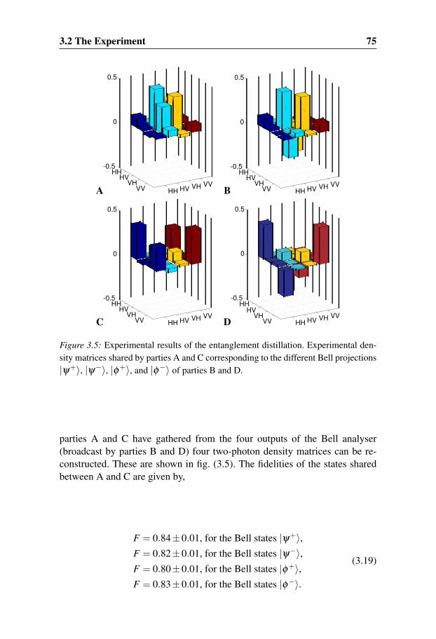
3.2 The Experiment 75
A B
C D
Figure 3.5: Experimental results of the entanglement distillation. Experimental den-sity matrices shared by parties A and C corresponding to the different Bell projections|ψ+〉, |ψ−〉, |φ+〉, and |φ−〉 of parties B and D.
parties A and C have gathered from the four outputs of the Bell analyser(broadcast by parties B and D) four two-photon density matrices can be re-constructed. These are shown in fig. (3.5). The fidelities of the states sharedbetween A and C are given by,
F = 0.84±0.01, for the Bell states |ψ+〉,F = 0.82±0.01, for the Bell states |ψ−〉,F = 0.80±0.01, for the Bell states |φ+〉,F = 0.83±0.01, for the Bell states |φ−〉.
(3.19)

76 Experimental Bound Entanglement
To determine whether the shared states are entangled we used the four two-qubit witnesses (1.15) and obtained,
Tr(Wψ+ ·ρexpψ+ ) =−0.198±0.017,
Tr(Wψ− ·ρexpψ− ) =−0.172±0.019,
Tr(Wφ+ ·ρexpφ+ ) =−0.141±0.015,
Tr(Wφ− ·ρexpφ− ) =−0.186±0.016,
(3.20)
with a theoretical value for all four witnesses of −0.5. These results clearlyshow that all four states are entangled.

77
4. Experiments on the Foundation ofQuantum Mechanics
In this chapter we describe how the four inequalities (1.24), (1.29), (1.33), and(1.37) can be tested experimentally. Our results were presented in articles IV,V, and VI. In all these experiments only single photons are used but we en-code four-levels (two-qubits) or three-levels (qutrit) in the single photons. Wedo this for two reasons: For one, we want to study the concept that a single en-tity can exhibit non-classical correlations between measurement results evenif no entanglement is present. Secondly it is practically impossible with cur-rent technology to perform several sequential measurement in a two-photonsystem.
For our sequential measurements we use two different types of schemes, acascaded (or space-encoded) and a time-encoded scheme. It is very importantin these measurements to keep the idea of a measurement box intact in allmeasurements. What do we mean by the term “measurement box” and whatis the idea behind it? For the first two inequalities, (1.24) and (1.29), we needto realise the nine observables (1.22) in the laboratory. Each one of these nineobservables is considered as contained in a physical measurement box, whichis a sorting machine of some sort. An eigenstate of an observable that entersthe box is sorted according to its eigenvalue +1 or −1. Any state entering abox can be expressed in the eigenstate basis of that box/observable and willbe sorted according to the probability of being in a state related to +1 and−1, respectively. The boxes can be connected in series to create a measure-ment sequence as required for sequential measurements. The important pointhere is that the same type of box (construction-wise) is used regardless of thecontext it is measured in. More precisely, consider the observables in (1.22)and the two measurement sequences ABC and Ccγ . If we construct a box Cwhen we measure C together with B and A, then the construction of box Cmust be the same when we measure C together with c and γ . This might seemtrivial at first but this means that we must distinguish between the productA ·B=(σz⊗11) ·(11⊗σz) and the observable C =σz⊗σz. Even though they aremathematically the same, they are contained in experimentally and conceptu-ally completely different boxes, a box where the product A ·B is measured isnot compatible with the observable c = σx⊗σx and γ = σy⊗σy, whereas C is

78 Experiments on the Foundation of Quantum Mechanics
Figure 4.1: Experimental scheme for a cascaded measurement. (a) shows the prepa-ration of a two-qubit state, its path and polarization. The state enters the first mea-surement box, x1, which sorts the state according to the eigenvalues of the observable.Depending on the eigenvalue the upper or the lower output is chosen. Each output isconnected to the next measurement box, x2, which again sorts according to the eigen-values of the observable. After the last box detectors are placed, the position of thedetectors now reveals the sequences of measurement outcomes. In (b) an idealizedmeasurement with lamps indicating the measurement outcome is shown. A descrip-tion of the individual components can be found in fig. (4.2).
compatible. The same holds for the observables Ai = 2|vi〉〈vi|− 11, where |vi〉are the vectors (1.35): each is thought of as a contained in a box that can beconnected whenever a measurement of the observable is desired.
The motivation for these experiments is to understand experimentally whatperforming a measurement means in a quantum system and how we can createsystems that produce outcomes that cannot have a classical interpretation. Wedo not attempt to construct loophole-free experiments. Instead, we give a proofof principle of how one can think and build experiments that keep importantquantum mechanical concepts intact.
In section 4.1 we present our experiments on the four-level system, i.e. twoqubits. This involves the two inequalities eqs. (1.24) and (1.29) and the cre-ation of the nine measurement boxes (1.22). After introducing the experimen-tal techniques used we present our results for the two inequalities and an upperbound for non-contextual content (1.27).
Following this, our experiments on the three-level system for the inequali-ties (1.33) and (1.37) are presented in section 4.2, where we also discuss thetime-bin measurement encoding we employed and our results.
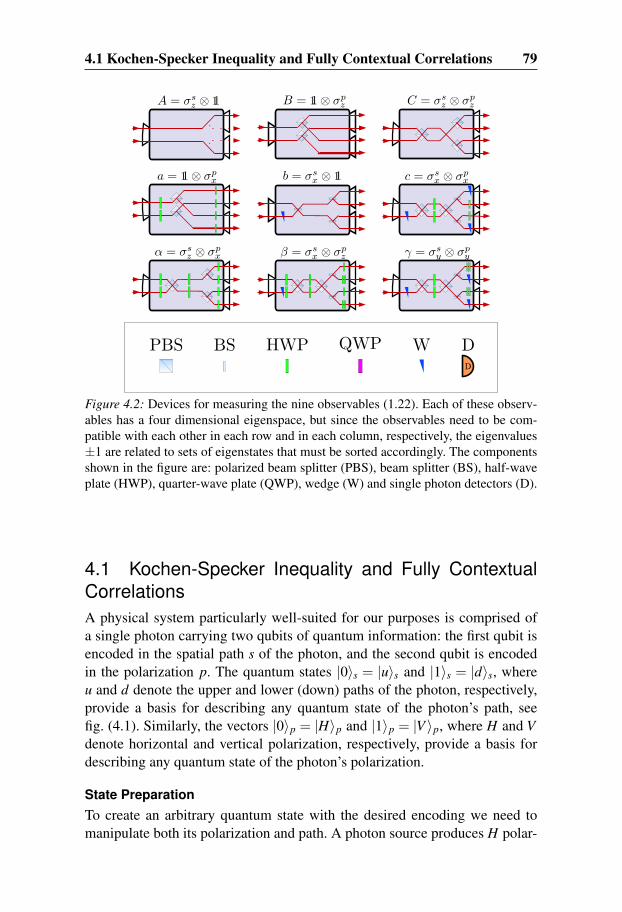
4.1 Kochen-Specker Inequality and Fully Contextual Correlations 79
Figure 4.2: Devices for measuring the nine observables (1.22). Each of these observ-ables has a four dimensional eigenspace, but since the observables need to be com-patible with each other in each row and in each column, respectively, the eigenvalues±1 are related to sets of eigenstates that must be sorted accordingly. The componentsshown in the figure are: polarized beam splitter (PBS), beam splitter (BS), half-waveplate (HWP), quarter-wave plate (QWP), wedge (W) and single photon detectors (D).
4.1 Kochen-Specker Inequality and Fully ContextualCorrelationsA physical system particularly well-suited for our purposes is comprised ofa single photon carrying two qubits of quantum information: the first qubit isencoded in the spatial path s of the photon, and the second qubit is encodedin the polarization p. The quantum states |0〉s = |u〉s and |1〉s = |d〉s, whereu and d denote the upper and lower (down) paths of the photon, respectively,provide a basis for describing any quantum state of the photon’s path, seefig. (4.1). Similarly, the vectors |0〉p = |H〉p and |1〉p = |V 〉p, where H and Vdenote horizontal and vertical polarization, respectively, provide a basis fordescribing any quantum state of the photon’s polarization.
State PreparationTo create an arbitrary quantum state with the desired encoding we need tomanipulate both its polarization and path. A photon source produces H polar-

80 Experiments on the Foundation of Quantum Mechanics
ized photons. By using a half-wave plate and a PBS we distribute the photonsproduced by this source into the two spatial paths u and d as desired. Usinghalf-wave and quarter-wave plates in each spatial path any polarization statecan be realised and a good control over the input state is achieved, as shownin the first block of fig. (4.1a).
In our experiment we used an attenuated continuous wave stabilized nar-row bandwidth (< 0.5nm) diode laser emitting at 780nm as the single-photonsource. The laser was attenuated such that the two-photon coincidences werenegligible. A mean photon number of 0.058 per time-window was estimatedthrough the count rate.
Measurement BoxAs mentioned above, a measurement box works like a sorting machine, thatis, the eigenstates of an observable are sorted according to their eigenvalues±1, see fig. (4.1). Note that each observable in (1.22) is generated with theeigenvalue spectrum +1,+1,−1,−1. Thus the diagonalisation of the oper-ator is not unique, any superposition of the two orthogonal states related to thetwo eigenvalue +1 is also related to the eigenvalue +1 and needs to be sentto that output. The same holds for the −1 eigenvalues. This way, each staterelated to the value +1 is sent to the upper output and will be distinguishablefrom the states related to the value −1 which are sent to the lower output offig. (4.1). As mentioned above, it is of utmost importance for our experimentthat the measurements of each of the nine observables in (1.22) are context-independent [16]. Thus care must be taken when designing the experiment inorder to enforce that the sorting is compatible for any context. We used themeasurement devices described in fig. (4.2) in our experiment, which satisfythis requirement of compatibility.
In detail the measurement boxes function as follows:Let us look at box A = σ s
z ⊗ 11 in fig. (4.2). Its eigenstates are given by|u〉s ⊗ |φ〉p and |d〉s ⊗ |φ〉p, where |φ〉p denotes any polarization state. Wewant to sort any state of this form into the two different outputs of our boxsince the states are coupled to the eigenvalues +1 and −1, respectively. Inthis case this sorting is accomplished easily, because the states are sorted onlyaccording to the path.
Box a = 11⊗σpx is a simple example for combining several ideas and meth-
ods. The eigenstates of a are the polarization states |ψ〉s⊗ |+〉p and |ψ〉s⊗|−〉p, where |ψ〉s is any path-encoded state. When one of these states entersthe measurement box a, we use a half-wave plate at 22.5 in both spatial pathsto rotate the polarization to the σz basis. Applying this rotation transforms theeigenstates into |ψ〉s⊗|H〉 and |ψ〉s⊗|V 〉. Now we can sort the states in eachpath according to their polarizations by using a PBS. If the polarizaton is H

4.1 Kochen-Specker Inequality and Fully Contextual Correlations 81
then the state is related to the value +1 and if it is V then it is related to thevalue−1. During all these operations one must always be careful to not disturbthe state encoded in the path, |ψ〉s. After the PBSs we have two sets of u and dpaths. One contains the states with horizontal polarization, the upper two, andone set with vertical polarizations, the lower two. Because of the polarizationtransformation these states are no longer eigenstates of the observable a. Tokeep the encoding between the boxes fixed and, more importantly, to preservethe box concept, we need to rotate the polarizations of the states back so theyagain become the eigenstates of the operator. Using a half-wave plate in eacharm set at 22.5 brings the states back into eigenstates. In terms of compatibil-ity, as long as we do not disturb the other degree of freedom then compatibilityis guaranteed.
As a last example and to illustrate the importance of the requirement ofcompatibility, let us look at box C = σ s
z ⊗σpz in fig. (4.2). The eigenstates of
C are |u〉s⊗ |H〉p, |d〉s⊗ |V 〉p, |u〉s⊗ |V 〉p, and |d〉s⊗ |H〉p, where two firsttwo states have the eigenvalues (+1) · (+1) and (−1) · (−1), respectively, andthe last two have the eigenvalues (+1) · (−1) and (−1) · (+1), respectively.Sorting must be implemented according to the product of the eigenvalues.However, expressing the eigenstates this way is very inconvenient, becauseit is assumed that we are in the σz basis and if one is not careful, describesA · B instead of C. It is more correct to write α|u〉s⊗ |H〉p + β |d〉s⊗ |V 〉p,and γ|u〉s⊗|V 〉p + δ |d〉s⊗|H〉p, where α , β , γ , and δ are arbitrary complexnumbers satisfying the normalization condition. The sorting must work forany state which is of the form stated above where the first state is associatedwith +1 and the second with −1.
Suppose the state α|u〉s⊗ |H〉p +β |d〉s⊗ |V 〉p enters the box C. Then thefollowing happens: The first part, |u〉s⊗ |H〉p, is transmitted in the PBS andthe second part , |d〉s⊗|V 〉p, is reflected. Everything is now in the same spatialpath, which is given by the lower center path in fig. (4.2), box C. If the spatialinterference and phases have been taken care of then the state can be assumedto have been transformed to |d〉s⊗ (α|H〉p +β |V 〉p). Thus we have convertedthe original state into a polarization state in the lower path d. For the othereigenstate related to −1 the same applies, except here everything is mappedto the upper arm. The two sets of eigenstates corresponding to the values ±1are now in two different paths and are distinguishable by the output channelof box C. But before they exit the box we need to reconstruct the eigenstates.This is easily done by using a PBS in the upper and lower paths before theyexit.
When connecting several boxes a large amount of interferometers are cre-ated, see article IV and the photograph of the set-up in fig. (4.4). For thisreason we needed to construct interferometers that are very stable but flexible,

82 Experiments on the Foundation of Quantum Mechanics
Figure 4.3: Two types of displaced Sagnac interferometers are shown. These whereused in our experimental realisation. The first (left) uses a 50/50 BS to split the beamand then a PBS to recombine the beams. For the second set-up (right) only one PBSis used. Observe that each beam hits every mirror.
since components need to be put inside the interferometers. All the interfer-ometers in the experimental set-up were based on free-space displaced Sagnacinterferometers, see fig. (4.3) and section 2.3.2. The advantage of using dis-placed Sagnac interferometers is that the beams are separated inside but stillhit all components. Thus if a phase is accumulated in one of the beams dueto mechanical vibrations, the other beam will also accumulate the same phaseand the unwanted effect cancels out. We achieved a visibility above 99% forour phase insensitive interferometers, and a visibility ranging between 90%and 95% for our phase sensitive interferometers.
Since the predictions of both non-contextual hidden variable theories andquantum mechanics do not depend on the order in which compatible mea-surements are performed, we chose the most convenient order for each setof observables (e.g., we measured CAB instead of ABC). The most conve-nient configuration was usually the configuration which minimized the num-ber of required interferometers and hence maximized visibility. Specifically,we measured the averages 〈CAB〉, 〈cba〉, 〈βγα〉, 〈αAa〉, 〈βbB〉, and 〈cγC〉, asdescribed in article IV.
We used single-photon detectors for the measurement, which were cali-brated to all have the same detection efficiency. All single counts were regis-tered using an eight-channel coincidence logic with a time window of 1.7ns.The main source of systematic errors was due to the large number of opticalinterferometers involved in the measurements, the non-perfect overlapping ofthe light modes, and the polarization components. The errors were deducedfrom propagated Poissonian counting statistics of the raw detection eventsand from 10 measurements over 10s to capture the fluctuation of the system.

4.1 Kochen-Specker Inequality and Fully Contextual Correlations 83
Figure 4.4: Photo of one of the set-ups. The measurement sequence is c, γ , and C.
The number of detected photons was about 1.7× 10⁶ per second. The mea-surement time for each of the six sets of observables was 10s for each state.
Since we studied a state-independent inequality a valid question might be:how can one not violate the inequality if the proper observables are used? Theviolation occurs since the coherence of the states from the output of each mea-surement box is kept undisturbed until the states reach the next box. If a distur-bance happens between the boxes then the observed amount of violation willbe smaller. Events that the theory treats as occurring between the boxes hap-pen inside the interferometers in the experiment. One way of thinking aboutthis is that the measurement box represents a mechanism for decoherence andit is between the boxes where we want to preserve coherence.
4.1.1 Results of the Experiment on the Kochen-SpeckerInequalityTo test the prediction of the state-independent inequality (1.24), we repeatedthe experiment on 20 quantum states of different purity and entanglement.For each pure state, we checked each of the six correlations in inequality(1.24). The results for the mixed states were obtained by suitably combin-ing pure state data. A detailed list of the results is shown in table (4.1) and anoverview of the results is displayed in fig. (4.5). Our results show that a state-independent violation of the inequality χ ≤ 4 occurs, with an average valuefor χ of 5.4521. Due to experimental imperfections, the experimental viola-

84 Experiments on the Foundation of Quantum Mechanics
Table 4.1: Experimental value of 〈CAB〉+〈cba〉+〈βγα〉+〈αAa〉+〈βbB〉−〈cγC〉 for20 quantum states. The average value is 5.4550± 0.0006 and on average we violatethe inequality with 655 standard deviations.
State Expectation value SD
|ψ1〉= 1√2(|t〉|H〉+ |r〉|V 〉) 5.4366 ± 0.0012 1169
|ψ2〉= 1√2(|t〉|H〉− |r〉|V 〉) 5.4393 ± 0.0023 621
|ψ3〉= 1√2(|t〉|V 〉+ |r〉|H〉) 5.4644 ± 0.0029 498
|ψ4〉= 1√2(|t〉|V 〉− |r〉|H〉) 5.4343 ± 0.0026 561
ρ5 =1316 |ψ1〉〈ψ1|+ 1
16 ∑4j=2 |ψ j〉〈ψ j| 5.4384 ± 0.0010 1386
ρ6 =58 |ψ1〉〈ψ1|+ 1
8 ∑4j=2 |ψ j〉〈ψ j| 5.4401 ± 0.0010 1509
ρ7 =7
16 |ψ1〉〈ψ1|+ 316 ∑
4j=2 |ψ j〉〈ψ j| 5.4419 ± 0.0010 1433
|ψ8〉= |t〉|H〉 5.3774 ± 0.0020 676
|ψ9〉= |t〉|V 〉 5.5131 ± 0.0032 475
|ψ10〉= |r〉|H〉 5.4306 ± 0.0031 465
|ψ11〉= |r〉|V 〉 5.4554 ± 0.0017 850
|ψ12〉= 1√2|t〉(|H〉+ |V 〉) 5.4139 ± 0.0015 960
|ψ13〉= 1√2|t〉(|H〉+ i|V 〉) 5.4835 ± 0.0022 667
|ψ14〉= 1√2(|t〉+ |r〉)|H〉 5.5652 ± 0.0032 489
|ψ15〉= 1√2(|t〉+ i|r〉)|H〉 5.5137 ± 0.0036 419
|ψ16〉= 12(|t〉+ |r〉)(|H〉+ |V 〉) 5.4304 ± 0.0014 1029
|ψ17〉= 12(|t〉+ i|r〉)(|H〉+ |V 〉) 5.2834 ± 0.0019 674
|ψ18〉= 12(|t〉+ |r〉)(|H〉+ i|V 〉) 5.5412 ± 0.0032 475
|ψ19〉= 12(|t〉+ i|r〉)(|H〉+ i|V 〉) 5.4968 ± 0.0032 462
ρ20 =14 ∑
4j=1 |ψ j〉〈ψ j| 5.4437 ± 0.0012 1229
tion of the inequality falls short of the quantum-mechanical prediction for anideal experiment (χ = 6). These results can also be used to give a bound forthe non-contextual content (1.27), using our best result we obtain WNC ≤ 0.22.Nevertheless, this is not the optimal way for generating non-contextual corre-lations because of the complexity of the experiment.

4.1 Kochen-Specker Inequality and Fully Contextual Correlations 85
Figure 4.5: State-independence of the violation of the inequality χ ≤ 4. The value of χ
was tested for 20 different quantum states from table (4.1) The solid red line indicatesthe classical upper bound. The dashed blue line at 5.4550 indicates the average valueof χ over all the 16 pure states.
4.1.2 Results on Fully Contextual CorrelationsThe result of the non-contextual correlations for inequality (1.24) gave an up-per bound for the non-contextual content of WNC ≤ 0.22. Another importantresult is the test with sequential measurements on a single photon in [65],which allows us to infer an upper bound for the non-contextual content ofWNC≤ 0.55. And for Bell type experiments the local content, which is the non-contextual content, an upper bounded of 0.22 was found in [41]. All these ex-periments are not optimised for the purpose of obtaining a low non-contextualcontent.
For inequality (1.29) only the observables (1.32) are needed. These aregiven by the two first columns of (1.22). We use the same experimental set-upas the Kochen-Specker set-up to measure the sequence of relevant operatorsin (1.32). The desired probabilities are given in (1.29). This can be achievedsince a we can always trace out the result of extra measurements made whenmeasuring (1.24). Our experimental results are shown in table (4.2). Theseresults lead to the following violation of inequality (1.29):
Ωexp = 3.4671±0.0010. (4.1)

86 Experiments on the Foundation of Quantum Mechanics
Table 4.2: Experimental results for the test of inequality (1.29).
Probability Experimental result
P(010|012) 0.24091±0.00021
P(111|012) 0.30187±0.00020
P(01|02) 0.28057±0.00020
P(00|03) 0.50375±0.00014
P(11|03) 0.47976±0.00014
P(00|14) 0.47511±0.00034
P(01|25) 0.43765±0.00015
P(010|345) 0.24296±0.00051
P(111|345) 0.25704±0.00052
P(10|35) 0.24751±0.00035
This result shows very good agreement with the quantum mechanical predic-tion, ΩQM = 3.5, and therefore provides an extremely low upper bound for thenon-contextual fraction of the correlations:
WNC ≤ 0.0658±0.0019. (4.2)
4.2 Klyachko et al. and WrightCompared to the previous experiments where two and four qubits were used,the experiments presented here require a three-level system that is a qutrit.This fact is of importance, and needs to be respected in the experiment, sinceour goal is to construct the simplest system that has a quantum advantage.Not only was our goal a violation of (1.33) and (1.37) but we also wanted toimprove the weaknesses of the set-up for the test of the Kochen-Specker in-equality. Our aim was to construct a system that offers, in a simple way, thepossibility to measure two operators in any order and simultaneously uses anon-cascaded structure in contrast to the Kochen-Specker experiment. By us-ing a time-bin encoding for marking the measurement results we were able toovercome the weakness of the previously used system. These changes unfor-tunately made the system more sensitive to vibrations. However, we believethat this could be improved further by a more compact system with bettercontrol in the aligning process. As before, it is crucial for the concept of the

4.2 Klyachko et al. and Wright 87
Figure 4.6: Experimental set-up for the experiment on the Wright inequality.(a)Scheme for single projective measurement Qi. The red and blue lamps correspondto unsuccessful (no) and successful (yes) projections, respectively. (b) Setup for cre-ating a qutrit and performing the time multiplexing measurement protocol. The de-tection is performed with single-photon detectors and a multi-coincidence countingunit, labelled C in the figure, which is triggered for all possible time slots by the pulsegenerator, labelled P in the figure, t0 and t1 = t0 +∆t. A click at the single photondetectors at time slots t0 (red) and t1 (blue) corresponds to unsuccessful (no) and suc-cessful (yes) projection measurements, respectively.(c) Definition for the symbols ofthe optical elements used in the setup: pulsed and attenuated laser diode (S), polariz-ing beam splitter (PBS), half-wave plate (HWP), quarter-wave plate (QWP), mirror(M), and single photon detector (D).
experiment that each measurement box, corresponding to the operators, is thesame in every context it is measured in.
The qutrit used is defined by means of the polarization and path degrees offreedom of a single photon in two spatial modes, labelled a and b, and suchthat, by design, the polarization in mode a is enforced to be horizontal (seefig. (4.6) and fig. (4.7)). The encoding is given by,
|0〉= |H,b〉, |1〉= |V,b〉, |2〉= |H,a〉, (4.3)
88 Experiments on the Foundation of Quantum Mechanics
where H denotes horizontal polarization and V denotes vertical polarization.This is a faithful implementation of a qutrit, since all qutrit states and projec-tive measurements, and only these, are accessible (that is, they can be preparedand measured) within the experiment.
State PreparationFor the qutrit preparation a pulse generator, labelled by P in fig. (4.6) andfig. (4.7), triggers the pulsed attenuated laser in the source, S. The set-up con-sists of a source of horizontally polarized photons which consists of a pulseddiode laser emitting at 780nm with a pulse width of 3ns and a repetition rate of100KHz. The laser was attenuated so that the two-photon coincidences werenegligible. This was followed by a half-wave plate and a polarizing beam split-ter, allowing us to prepare any probability distribution of a photon in modes aand b. A half-wave plate (HWP) and a quarter-wave plate (QWP) in mode ballow us to rotate the reflected outputs of the polarizing beam splitter to anypolarization.
Measurement BoxThe questions Qi for testing inequality (1.33) are represented by the 5 pro-jectors constructed by the vectors in (1.35). For the second inequality (1.37),two sequential measurements corresponding to the pairwise compatible ob-servables Ai and Ai±1 need to be performed. Each of the observables Ai for thetest of inequality (1.37) is a function, Ai = 2|vi〉〈vi|− 11, of the correspondingprojector Qi. Experimentally, there is no difference between measuring Qi andAi, except that we assign the values (±1) to a successful and non-successfulprojection, respectively, for the latter measurement. The assignment is madeaccording to the eigenvalues of the operator Ai to be able to evaluate the ex-pectation value, whereas for the Qi we are only interested in the probabilitiesof the events.
To understand the concept of the set-up let us explain how a general mea-surement box works in this case. Different eigenvalues of an operator are allpossible outcomes and these are marked with a time multiplexing scheme. Apositive answer corresponds to a successful projection and is indicated by thetime arrival t1 of the photon (or by a blue lamp flashing in the Mermin boxnotation; see fig. (4.6) and fig. (4.7) ), a negative answer corresponds to anunsuccessful projection and is indicated by the time arrival t0 of the photon(or a red lamp flashing; see fig. (4.6) and fig. (4.7)). The state with a positiveeigenvalue (the projecting state in Qi, (1.35)) is mapped onto the state |H,b〉,and any orthogonal state is mapped onto a state on the plane orthogonal to|H,b〉, which we denote by |H,b〉⊥. These two states are distinguished byintroducing a time delay ∆t = t1− t0 between them.

4.2 Klyachko et al. and Wright 89
Figure 4.7: Experimental set-up for the Klyachko experiment for sequential measure-ments. (a) Scheme for sequential measurement on pairwise compatible observablesAi and Ai+1. The red and blue lamps correspond to the eigenvalue −1 (no) and +1(yes), respectively. (b) Set-up for performing sequential measurements Ai and Ai+1.The input qutrit state is defined in the spatial modes a and b as in fig. (4.6). The firstmeasurement is exactly the same as described in fig. (4.6). The eigenstates of Ai witheigenvalues +1 and −1 are mapped to orthogonal states. The same-time multiplex-ing detection method described in the text is used here to distinguish between the +1and−1 eigenvalues. The input state is re-prepared in the eigenstate of the observablebefore entering Ai+1. In the second measurement, the delay time is set to 2∆t. A clickat the detectors at the time slots t0 = t i
0 + t i±10 , t1 = t0 +∆t i, t2 = t0 +∆t i±1, and
t3 = t0 +∆t i +∆t i±1 corresponds to the answers (no, no), (yes, no), (no, yes) and(yes, yes), respectively. The preparation of the qutrit state and the symbols are thesame as in fig. (4.6).
Conceptually and ideally the time delay will distinguish between the pos-itive eigenvalue state in (1.35) and the orthogonal plane without the need ofthe mapping mentioned above. Furthermore, the output of the measurementbox is supposed to be given by the eigenstates entangled with some extra tim-ing information that we can easily read off later. This is important becausewe would like to use the same encoding convention (4.3) for the input of thesecond box, if we put a second measurement box after the first measurement.Moreover, if the second box is to measure the same operator as the first onethen the boxes need to be identical in construction to keep the context conceptvalid. To satisfy this ideal measurement condition we remap each state |H,b〉and |H,b〉⊥ back to its original state before it exits the measurement box.

90 Experiments on the Foundation of Quantum Mechanics
More precisely, if we follow the evolution of a pure state entering a generalmeasurement device of fig. (4.6) then we have the following situation: Anyinput qutrit state can be expressed as |φ〉= α|H,b〉+β |V,b〉+ γ|H,a〉, whereα,β and γ are complex numbers. Suppose that we want to measure the op-erator O = 2|φ〉〈φ | − 11. Then the first step is to choose as an input the statecorresponding to the state appearing in the projector |φ〉〈φ |. Then we rotatethe polarization in mode b to obtain the state β ′|V,b〉+ γ|H,a〉. In the set-upof fig. (4.6) this is the first HWP marked by θi. This can always be done sincethe rotation of the polarization is performed only in mode b. Secondly, wetransfer the part of the state in mode a into mode b, this process also flips thepolarization of the two modes a and b. This leads to the state β ′|H,b〉+γ|V,b〉if the phase of the interferometer is set correctly. The state of mode b can nowbe rotated to |H,b〉 by a HWP, in fig. (4.6) this is marked with 21. Finally,it is easy to separate |H,b〉 from |H,b〉⊥ by a PBS and add a delay by ∆t todistinguish it from the orthogonal states at the time slots t1 and t0. After thisprocedure all previous steps (except the time delays) are performed in reverseorder to re-prepare the eigenstate of the observable for further processing. Anyqutrit dichotomic measurement can be constructed by this mapping procedureby introducing the proper polarization rotations for the two HWP’s marked θi
and 21 in fig. (4.6) together with the proper re-preparation.The detection is performed with single-photon detectors and a
multi-coincidence counting unit, labelled C in fig. (4.6) and fig. (4.7),which is triggered for all possible time slots by the pulse generator, t0 andt1 = t0 +∆t. A click at the single photon detectors at time slots t0 (red) andt1 (blue) corresponds to unsuccessful (no) and successful (yes) projectionmeasurements, respectively.
A useful property of the set-up is that the devices for measuring each of the5 operators Qi and Ai are exactly the same, up to a half-wave plate rotation,see fig. (4.6) and fig. (4.7). To apply one of the five operators Qi and Ai, werotate both the first and last half-wave plate by an angle θi = 45, 117, 9,81, and 153 for i = 0, i = 1, i = 2, i = 3, and i = 4, respectively.
For the Klyachko inequality sequential measurements are required. Becauseof the time multiplexing and re-preparation we only need to use two set-upsin sequence, see fig. (4.7). In the second measurement, the time delay is setto 2∆t to not overlap with the time slot of the first measurement. A click atthe detectors at the time slots t0 = t i
0 + t i±10 , t1 = t0 +∆t i, t2 = t0 +∆t i±1, and
t3 = t0 +∆t i +∆t i±1 corresponds to the answers (no, no), (yes, no), (no, yes),and (yes, yes), respectively (see fig. (4.7)), where the upper index indicatesonly from which operator Ai the time delay is accumulated from.

4.2 Klyachko et al. and Wright 91
Table 4.3: Experimental results for the violation of inequality (1.33), W ≤ 2.
P(+1|Q0) 0.4600±0.012
P(+1|Q1) 0.4544±0.012
P(+1|Q2) 0.4603±0.016
P(+1|Q3) 0.4610±0.011
P(+1|Q4) 0.4566±0.010
W 2.292±0.028
4.2.1 Results on Klyachko et al. and WrightThe actual set-up in the lab had the structure as shown in fig. (4.6) andfig. (4.7). Each interferometer had a visibility ranging between 80% and 90%.All single-detection counts and the time delayed trigger signals (defining themeasurement time slots) were registered using multichannel coincidencelogic with a time window of 1.7ns. The number of detected photons wasapproximately 3 ·104 per second. The measurement time for each observablewas 1s per run.
The experimental results for the test of Wright inequality (1.33) are shownin table (4.3). We observe a clear violation of inequality (1.33) in good agree-ment with the predictions of quantum mechanics. The fact that the experimen-tal value is slightly larger than the maximum quantum value can be explainedby the fact that the latter is obtained under the assumption that the measuredpropositions are (perfectly) exclusive. This condition is enforced experimen-tally by measuring projectors which are not exactly (only approximately) theones required by the theory.
Our experimental results for the test of inequality (1.37) are shown in table(4.4). The measurements were performed in all possible orders to confirm thatthe violation does not dependent on the order. The experimental results intable (4.4) show a clear violation of inequality (1.37), in good agreement withthe theoretical prediction for the maximal quantum violation.
Because of experimental imperfections, the observed violation of both in-equalities fall slightly short of the quantum mechanical prediction for an idealexperiment. The main sources of systematic error were due to the optical in-terferometers involved in the measurements, the imperfect overlapping andcoupling of the light modes, and the polarization components. The errors werededuced from propagated Poissonian counting statistics of the raw detectionevents.

92 Experiments on the Foundation of Quantum Mechanics
Table 4.4: Experimental results for the violation of inequality (1.37) κ ≤ 3.
〈A0A1〉 −0.712±0.002 〈A1A0〉 −0.785±0.003
〈A1A2〉 −0.706±0.002 〈A2A1〉 −0.781±0.003
〈A2A3〉 −0.704±0.002 〈A3A2〉 −0.774±0.003
〈A3A4〉 −0.708±0.002 〈A4A3〉 −0.774±0.003
〈A4A0〉 −0.706±0.002 〈A0A4〉 −0.782±0.003
κ −3.536±0.005 κ −3.896±0.006

93
5. Conclusions and Outlook
In this thesis we have investigated how quantum correlations can be generatedand transformed by noise. We have considered and experimentally tested twomain topics.
First we studied bound entangled states, where we investigated the effect ofa noise channel on a pair of bipartite entangled states. The dynamics of entan-glement was demonstrated by increasing the strength of several types of noise.We showed that it is indeed possible to create bound entangled states and toviolate a CHSH-type inequality even in this bound regime. We concluded ourexperimental investigation of this topic by demonstrating the unlocking ofentanglement through an extraction of the entanglement for two of the fourparties involved.
In the second part we presented several tests of quantum correlations insingle-photon systems. The inequalities under study were derived under theassumption of non-contextuality. We emphasised several counter-intuitive as-pects of quantum mechanics. We experimentally demonstrated the state in-dependence of the Kochen-Specker theorem for a four-level system and gen-erated correlations with a small amount of non-contextual content. We alsodemonstrated in two experiments involving a three-level system the discrep-ancy between classical and quantum physics.
Bound EntanglementOur goal was to study if it is possible with the currently available technol-ogy to create exotic bound entangled states. These states have the property ofnot being distillable after being distributed to parties that can only performlocal operations and can only communicate with each other through classicalcommunication channels. We transformed our pure input state into a mixedstate via a noisy channel. Because we had control over the amount of errorintroduced in this channel we were able to study the decoherence behaviourof an input state with increased noise. Specifically, we considered four typesof noisy channels which enabled us to transform our input state into a boundentangled regime.
We explored this exotic behaviour through double-pass parametric down-conversion. In this experiment we studied second order terms and used post-

94 Conclusions and Outlook
selection criteria for filtering out four-photon events. By proper walk-off com-pensation combined with spectral and spatial filtering we were able to obtainthe product of two singlet states. Furthermore, we created all other sixteencombinations of Bell states in our noisy channel by motorized tilting of thecompensation crystals and half-wave plates mounted on motorized rotationstages. The use of a computer as our random number generator enabled usto create any desired statistical mixture of all sixteen Bell states. In order tocharacterize the state and its entanglement properties we performed a quantumstate tomography, and employed the witness method and a CHSH-inequality.The density matrix was reconstructed by a maximum likelihood method. Thisrevealed states with high-fidelity, close to the theoretical expectation.
The signature of bound entanglement is a positive partial trace of the stateunder consideration. By calculating eigenvalues of the partial trace for all bi-partite cuts we were able to see when the state entered the bound entangledregime. Our study showed that our noisy channel can bring states into a boundregime and that the CHSH-inequality is very close to being violated. We stud-ied the noisy channel that created the largest CHSH-value while still produc-ing states with a positive partial transpose in order to probe the boundary ofthe CHSH-inequality. We where able to increase the CHSH-value to a achieveviolation of the inequality by optimizing the parameters of the error-channeland adding a small perturbation to the parameters of the channel by hand.
Aside from this characterisation of the state we implemented a two-partydistillation protocol where two parties join each other to perform a Bell mea-surement. In this study we used a sign-shift gate which utilizes the photonbunching effect. This way we achieved a complete passive Bell measurement.The remaining parties gathered all measurement data required for a tomo-graphical reconstruction of the density matrix sorted by the outcome of theBell measurement. By using the entanglement witness method we showedthat entanglement is present in the distilled states.
The experimental investigation of the effects of correlated error channelson quantum states has only recently become of interest and much can still belearned. Several other research groups have achieved bound entanglement ina variety of systems [64, 66–68]. In all these cases the bound entanglementis generated by relatively artificial means. An appealing approach to generatethese states is to consider larger pure quantum states where the bound regimeis reached by tracing out some of the parties. Here the error of losing a qubitoccurs quite naturally, and the results of our studies may be important for thesecases.

95
Foundation of Quantum MechanicsWe performed four tests of quantum mechanics based on the assumption ofnon-contextuality. In all tests we used path and polarization encoding to en-code a four- or three-level system into one photon. We performed two typesof measurements, for the four-level system we employed a cascaded mea-surement scheme where the path of the photon revealed the measurement se-quence. The second scheme, used for the three-level system, was based ontime encoding where the arrival time of the photon at the detector marked themeasurement sequence. Using nested interferometers and polarization opticsto implement these encoding schemes we could sequentially measure the ef-fects of various quantum operators. With the cascaded set-up we showed thestate independence of the Kochen-Specker theorem by violating an inequalityfor 20 states that included the completely mixed state. Furthermore, we founda very small bound for the non-contextual content. With the time-encoded set-up we demonstrated through direct and sequential measurements the simplestsystem with a discrepancy between classical and quantum results.
All these tests illustrate different non-intuitive aspects of quantum mechan-ics. Aside from addressing the more fundamental questions, which theory andexperiments are trying to shed new light on, it is possible to use these ideasfor more practical purposes, such as device-independent quantum key dis-tribution [69, 70] and random number generation [71]. All of these applica-tions require a spacelike separation between the parties involved. In addition,quantum contextuality also offers applications in scenarios without spacelikeseparation. Examples are the reduction of communication complexity [72],parity-oblivious multiplexing [73], improving zero-error classical communi-cation [74], and quantum cryptography that is secure against specific attacks[75]. In our experiments we explored issues that are important for the afore-mentioned applications.


97
Bibliography
[1] A. Einstien, B. Podolsky, and N. Rosen. Can quantum-mechanical descriptionof physical reality be considered complete? Phys. Rev., 47, 1935.
[2] J. Bell. On the einstein podolsky rosen paradox. Physics, 1:195, 1964.
[3] S. Kochen and E. Specker. The problem of hidden variables in quantum me-chanics. J. Math. Mech., 17:59, 1967.
[4] J. F. Clauser, M. A. Horne, A. Shimony, and R. A. Holt. Proposed experimentto test local hidden-variable theories. Phys. Rev. Lett., 23(15):880, 1969.
[5] Alain Aspect, Jean Dalibard, and Gérard Roger. Experimental test of bell’sinequalities using time- varying analyzers. Phys. Rev. Lett., 49, 1982.
[6] A. Aspect, P. Grangier, and G. Roger. Experimental realization of einstein-podolsky-rosen-bohm gedankenexperiment: A new violation of bell’s inequali-ties. Phys. Rev. Lett., 49, 1982.
[7] M. A. Nielsen and I. L. Chuang. Quantum Computation and Quantum In-formation. Cambridge University Press, 2000.
[8] C. H. Bennett, G. Brassard, S. Popescu, B. Schumacher, J. A. Smolin, andWilliam K. Wootters. Purification of noisy entanglement and faithful telepor-tation via noisy channels. Phys. Rev. Lett., 76:722, 1996.
[9] C. H. Bennett, H. J. Bernstein, S. Popescu, and B. Schumacher. Concentratingpartial entanglement by local operations. Phys. Rev. A, 53:2046, 1996.
[10] M. Horodecki, P. Horodecki, and R. Horodecki. Mixed-state entanglement anddistillation: Is there a "bound" entanglement in nature? Phys. Rev. Lett., 80(24):5239, 1998.
[11] R. Augusiak and P. Horodecki. Bound entanglement maximally violating bellinequalities: Quantum entanglement is not fully equivalent to cryptographic se-curity. Phys. Rev. A, 74, 2006.
[12] W. Dür. Multipartite bound entangled states that violate bell’s inequality. Phys.Rev. Lett., 87:230402, 2001.

98 BIBLIOGRAPHY
[13] J. A. Smolin. Four-party unlockable bound entangled state. Phys. Rev. A, 63:032306, 2001.
[14] Y. Huang1, C. Li1, Y. Zhang, J. Pan, and G. Guo. Experimental test of thekochen-specker theorem with single photons. Phys. Rev. Lett., 90:250401,2003.
[15] Y. Hasegawa1, R. Loidl, G. Badurek, M. Baron, and H Rauch. Violation of abell-like inequality in single-neutron interferometry. Nature, 425:45, 2003.
[16] A. Cabello. Experimentally testable state-independent quantum con-textuality.Phys. Rev. Lett., 101:210401, 2008.
[17] A. Cabello, S. Severini, and A. Winter. (non-)contextuality of physical theoriesas an axiom. arxiv, 2010. 1010.2163.
[18] J. Lavoie, R. Kaltenbaek, M. Piani, and K. J. Resch. Experimental bound entan-glement? Nature Physics, 6:827, 2010.
[19] C. E. Shannon. Mathematical theory of communication. The Bell SystemTechnical Journal, 27:379, 1948.
[20] V. Vedral, M. B. Plenio, M. A. Rippin, and P. L. Knight. Quantifying entangle-ment. Phys. Rev. Lett., 78(12):2275, 1997.
[21] A. Peres. Separability criterion for density matrices. Phys. Rev. Lett., 77(8),1996.
[22] M. Horodecki, P. Horodecki, and R. Horodecki. Inseparable two spin- 12 density
matrices can be distilled to a singlet form. Phys. Rev. Lett., 78(4), 1996.
[23] P. Horodecki. Separability criterion and inseparable mixed states with positivepartial transposition. Phys. Lett. A, 232:333, 1997.
[24] M. Horodecki, P. Horodecki, and R. Horodecki. Separability of mixed states:necessary and sufficient conditions. Phys. Lett. A, 223:1, 1996.
[25] M. Lewenstein, B. Kraus, J. I. Cirac, and P. Horodecki. Optimization of entan-glement witnesses. Phys. Rev. A, 62:052310, 2000.
[26] G. Tóth and O. Gühne. Entanglement detection in the stabilizer formalism.Phys. Rev. A, 72:022340, 2005.
[27] O. Gühne, P. Hyllus, D. Brub, A. Ekert, M. Lewenstein, C. Macchiavello, andA. Sanpera1. Detection of entanglement with few local measurements. Phys.Rev. A, 66:062305, 2002.

BIBLIOGRAPHY 99
[28] M. Bourennane, M. Eibl, C. Kurtsiefer, S Gaertner, H. Weinfurter, O. Gühne,P. Hyllus, D. Brub, M. Lewenstein, and A. Sanpera. Experimental detection ofmultipartite entanglement using witness operators. Phys. Rev. Lett., 92, 2004.
[29] E. Schrödinger. Discussion of probability relations between separated systems.Proc. Cambridge Philos. Soc., 31:555, 1935.
[30] N. Bohr. Can quantum-mechanical description of physical reality be consideredcomplete? Phys. Rev., 48:696, 1935.
[31] J. Bell. On the problem of hidden variables in quantum mechanics. Rev. Mod.Phys., 38:447, 1966.
[32] E. Specker. Die logik nicht gleichzeitig entscheidbarer aussagen. Dialectica,14:239, 1960. Translated version arXiv:1103.4537.
[33] J. F. Clauser and M. A. Horne. Experimental consequences of objective localtheories. Phys. Rev. D, 10(2):526, 1974.
[34] J. L. Cereceda. Quantum mechanical probabilities and general probabilisticconstraints for einstein-podolsky-rosen-bohm experiments. Foundations ofPhysics Letters, 13(5):427, 2000.
[35] M. Hillery and B. Yurke. Bell’s theorem and beyond. Quantum Semiclass.Opt., 7:215, 1995.
[36] R. F. Werner and M. M. Wolf. Bell inequalities and entanglement. QuantumInf. Comput., 1(3):1, 2001.
[37] J. Barrett, A. Kent, and S. Pironio. Maximally nonlocal and monogamous quan-tum correlations. Phys. Rev. Lett., 97:170409, 2006.
[38] B. S. Cirelson. Quantum generalizations of the bell’s inequality. Lett. Math.Phys., 4:93, 1980.
[39] A. Peres. Quantum Theory: Concepts and Methods. Kluwer Academic,1995.
[40] D. Mermin. Simple unified form of the major no-hidden-variable theorems.Phys. Rev. Lett., 49, 1990.
[41] L. Aolita, R. Gallego, A. Acín, A. Chiuri, G. Vallone, P. Mataloni, and A. Ca-bello. Fully nonlocal quantum correlations. arxiv, 2011. 1105.3598v1.
[42] S. Popescu and D. Rohrlich. Quantum nonlocality as an axiom. Foundationsof Physics, 24(3):379, 1994.

100 BIBLIOGRAPHY
[43] A. A. Klyachko, M. A. Can, S. Binicioglu, and A. S. Shumovsky. Simple testfor hidden variables in spin-1 systems. Phys. Rev. Lett., 101:020403, 2008.
[44] R. Wright. Mathematical foundations of quantum theory. Academic Press,1978. pp.255-274.
[45] C. Lu, X. Zhou, O. Gühne, W. Gao, J. Zhang, Z. Yuan, A. Goebel, T. Yang,and J. Pan. Experimental entanglement of six photons in graph states. NaturePhysics, 3:91, 2007.
[46] M. Rådmark, M. Zükowski, and M. Bourennane. Experimental test of fidelitylimits in six-photon interferometry and of rotational invariance properties of thephotonic six-qubit entanglement singlet state. Phys. Rev. Lett., 103:150501,2009.
[47] R. Paschotta. Encyclopedia of laser physics and technology. rp-photonics,2008. http://www.rp-photonics.com/fibers.html.
[48] A. Zilinger. General properties of lossless beam splitters in interferometry. Am.J. Phys., 49:090882–2, 1981.
[49] T. C. Ralph, N. K. Langford, T. B. Bell, and A. G. White. Linear opticalcontrolled-not gate in the coincidence basis. Phys. Rev. A, 65:062324, 2002.
[50] J. L. O’Brien, G. J. Pryde, A. G. White, T. C. Ralph, and D. Branning. Demon-stration of an all-optical quantum controlled-not gate. Nature, 426, 2003.
[51] H. F. Hofmann and S. Takeuchi. Quantum phase gate for photonic qubits usingonly beam splitters and postselection. Phys. Rev. A, 66:024308, 2002.
[52] N. Kiesel, C. Schmid, U. Weber, R. Ursin, and H. Weinfurter. Linear opticscontrolled-phase gate made simple. Phys. Rev. Lett., 95:210505, 2005.
[53] J. Alda. Laser and gaussian beam propagation and transformation. Encyclope-dia of Optical Engineering, page 999, 2003.
[54] T. F. Johnston. Beam propagation (M2) measurement made as easy as it gets:the four-cuts method. Appl. Opt., 37:4840, 1998.
[55] PerkinElmer. Avalanche photodiode, A User Guide. PerkinElmer, 2008.http://optoelectronics.perkinelmer.com.
[56] J.J. Sakurai. Modern Quantum mechanics. Addison Wesley, revised ed. edi-tion, 1994.
[57] J. B. Altepeter, E. R. Jeffrey, and P. G. Kwiat. Advances in Atomic, Molecular,and Optical Physics. Elsevier, 2005. pp.105–159.

BIBLIOGRAPHY 101
[58] D. James, P. G. Kwiat, W. J. Munro, and A. G. White. Measurement of qubits.Phys. Rev. A, 64:052312, 2001.
[59] R. Augusiak and P. Horodecki. Generalized smolin states and their properties.Phys. Rev. A, 73, 2006.
[60] C. Brukner, M. Zukowski, J. Pan, and A. Zeilinger. Bell’s inequalities and quan-tum communication complexity. Phys. Rev. Lett., 92, 2004.
[61] M. Murao and V. Vedral. Remote information concentration using a bound en-tangled state. Phys. Rev. Lett., 86:352, 2001.
[62] R. Horodecki and M. Horodecki. Information-theoretic aspects of inseparabilityof mixed states. Phys. Rev. A, 54:1838, 1996.
[63] B. C. Hiesmayr, F. Hipp, M. Huber, P. Krammer, and Ch. Spengler. Simplex ofbound entangled multipartite qubit states. Phys. Rev. A, 78:042327, 2008.
[64] J. Lavoie, R. Kaltenbaek, M. Piani, and K. J. Resch. Experimental bound entan-glement in a four-photon state. Phys. Rev. lett., 105:130501, 2010.
[65] R. Łapkiewicz, C. Schaeff P. Li, N. Langford, S. Ramelow, M. Wiesniak, andA. Zeilinger. Experimental non-classicality of an indivisible quantum system.Nature, 474:490, 2011.
[66] J. T. Barreiro, P. Schindler, O. Gühne, T. Monz, M. Chwalla, C. F. Roos, M. Hen-nrich, and R. Blatt. Experimental multiparticle entanglement dynamics inducedby decoherence. Nature Physics, 6:943, 2010.
[67] H. Kampermann, D. Bruß, X. Peng, and D. Suter. Experimental generation ofpseudo-bound-entanglement. Phys. Rev. A, 81:040304(R), 2010.
[68] J. DiGuglielmo, A. Samblowski1, B. Hage1, C. Pineda, J. Eisert, and R. Schn-abel. Preparing the bound instance of quantum entanglement. ArXiv, 2010.[arXiv:1006.4651v2].
[69] J. Barrett, L. Hardy, and A. Kent. No signaling and quantum key distribution.Phys. Rev. Lett., 95:010503, 2005.
[70] A. Acín, N. Brunner, N. Gisin, S. Massar, S. Pironio, and V. Scarani. Device-independent security of quantum cryptography against collective attacks. Phys.Rev. Lett., 98:230501, 2007.
[71] S. Pironio, A. Acín, S. Massar, A. Boyer de la Giroday, D. N. Matsukevich,P. Maunz, S. Olmschenk, D. Hayes, L. Luo, T. A. Manning, and C. Monroe.Random numbers certified by bell’s theorems. Nature, 464:1021, 2010.

102 BIBLIOGRAPHY
[72] H. Buhrman, R. Cleve, S. Massar, and R. de Wolf. Nonlocality and communi-cation complexity. Rev. Mod. Phys., 82:665, 2010.
[73] R. W. Spekkens, D. H. Buzacott, A. J. Keehn, B. Toner, and G. J. Pryde. Prepara-tion contextuality powers parity-oblivious multiplexing. Phys. Rev. Lett., 102:010401, 2009.
[74] T. S. Cubitt, D. Leung, W. Matthews, and A. Winter. Improving zero-error clas-sical communication with entanglement. Phys. Rev. Lett., 104:230503, 2010.
[75] A. Cabello, V. D’Ambrosio, E. Nagali, and F. Sciarrino. Hybrid ququart-encoded quantum cryptography protected by kochen-specker contextuality.Phys. Rev. A, 84:030302(R), 2011.

Part II:Scientific Publications