Dynamics of Innovation and Risk

December 2014

Bruno Biais

Toulouse School of Economics (CNRS-CRM and IDEI-PWRI)

Jean-Charles Rochet

University of Zurich and Toulouse School of Economics

Paul Woolley

London School of Economics

Many thanks for thoughtful comments to the Editor, David Hirshleifer, and two referees, as well as

the participants in the first conference of the Centre for the Study of Capital Market Dysfunctionality

at the London School of Economics, the Pompeu Fabra Conference on the Financial Crisis, the third

Banco de Portugal conference on Financial Intermediation, the Europlace Institute of Finance 7th

Annual Forum, and seminars at London Business School, Frankfurt University, the European Central

Bank and Amsterdam University. Rochet acknowledges support from the European Research Council

(24915-RMAC) and from NCCR Finrisk. Biais acknowledges financial support from the European

Research Council under the European Community’s Seventh Framework Program (FP7/2007-2013

grant agreement 295484.) Send correspondence to Bruno Biais, Toulouse School of Economics, 21

1

allée de Brienne, 31000 Toulouse, France; telephone: 33 5 61 12 85 98. E-mail: bruno.biais@univ-

tlse1.fr.

2

Abstract

We study the dynamics of an innovative industry in which agents learn about the likelihood of

negative shocks. Managers can exert risk prevention effort to mitigate the consequences of shocks.

If no shock occurs, confidence improves, attracting managers to the innovative sector. But, when

confidence becomes high, ineffi cient managers exerting low risk-prevention effort also enter. This

stimulates growth, while reducing risk prevention. The longer the boom, the larger the losses if

a shock occurs. Although these dynamics arise in the first-best, asymmetric information generates

excessive entry of ineffi cient managers, earning informational rents, inflating the innovative sector,

and increasing its vulnerability. (JEL D82, D86, G01, G2)

3

As vividly illustrated by the boom and bust of the financial sector in the recent decade, innovations

can spur rapid growth, as well as declining standards, accumulated risk, and finally crises. The goal of

this paper is to shed light on the dynamics of innovations and risk. Innovations are, by their very na-

ture, initially untested. Market participants are initially uncertain about the strength, potential, and

workings of an innovation.1 They progressively learn about it. Innovative resecuritization techniques

offer a good illustration of initial uncertainty and the scope for learning. Collateralized debt obliga-

tions of asset backed securities offered new ways to reallocate risk, potentially enhancing risk sharing

and liquidity. But the reliability and effectiveness of this innovation was not fully clear ex ante. It

depended, in particular, on the degree of correlation between the property markets in different Amer-

ican cities, a parameter for which there was uncertainty. Awareness of uncertainty about the strength

of financial innovations was displayed in a “School Brief”published in 1999 by The Economist : “Some

of the new financial technologies are, in effect, efforts to bottle up considerable uncertainties. If they

work, the world economy will be more stable. If not, an economic disaster might ensue.”(qtd in The

Economist, September 7, 2013, 57).

Motivated by these stylized facts, we study uncertainty and learning about the fragility of an

innovative industry, that is, the likelihood that it is hit by negative shock. More precisely, we assume

that, with some probability the innovation is strong, whereas with the complementary probability

it is weak. When the innovation is weak, there is a significant risk of negative aggregate shocks,

reducing the productivity of all projects in the innovative sector. When the innovation is strong, the

1We focus on Bayesian uncertainty, where agents learn about the parameters of a well—defined model. This differsfrom Knightian uncertainty, studied by, for example, Caballero and Krishnamurthy (2008).

4

likelihood of such negative shocks is lower. As long as there is no aggregate shock, confidence in the

strength of the innovation increases. This leads to an increase in the size of the innovative sector. In

contrast, when negative shocks occur, this generates pessimism and leads to a decline in the size of

the innovative sector.2

Our model features managers and investors. The latter can invest in the traditional sector or

the innovative one. Because the traditional sector is well known, investors can directly manage their

investments in that sector. In contrast, investment in the innovative sector is more challenging. While

managers know how to operate in that sector, investors do not. Hence, when opting for the innovative

sector, investors must delegate the care of their investments to managers. Thus, investors are princi-

pals, while managers are their agents. Correspondingly, we hereafter take the terms “managers”and

“agents”as synonymous.

Agents managing investments in the innovative sector can exert costly risk prevention effort, to

reduce downward risk. This is in line with investment situations with bounded upside in which the

key is to prevent an unusually low downside. This applies, in general, to the need for due diligence

in the purchase of assets, whereby failure to inspect an asset may fail to uncover some hidden flaw.

This fits particularly well the purchase of fixed income securities. For example, when investing in a

portfolio of Collateralized debt obligations, or high-yield bonds, the manager can carefully scrutinize

the quality of the paper in which he invests. Alternatively, if not exerting risk prevention effort, the

manager relies on ready-made evaluations, such as those obtained from credit rating agencies. We

2Thus, our analysis is in line with that of Zeira (1987, 1999), Rob (1991), Pastor and Veronesi (2006), and Barbarinoand Jovanovic (2007), who show that learning induces fluctuations in industry size.

5

consider a continuum of heterogeneous managers. Some have effi cient risk management systems, so

that, for them, risk prevention effort is not very costly. Others have less effi cient risk management

systems and incur larger costs when they exert risk prevention effort.

Our key assumption is that the benefits of risk prevention effort materialize when the innovation is

subsequently hit by a negative shock. When there is no negative shock, innovative projects fare well,

even when managers exerted low effort. When a negative shock hits, the projects whose managers

exerted large risk prevention effort are relatively robust, whereas the other projects are highly likely

to fail. This assumption fits the stylized facts from the Tech boom and bust. Market participants

who invested without careful scrutiny in dot.com ventures fared relatively well until the bust of March

2000, but then incurred large losses. Another example is momentum-like trading, where, instead of

conducting fundamental analysis, fund managers invest in stocks that previously fared well. While

such strategy can generate profits in lenient market environments, it runs the risk of large losses

when the market is hit by a negative shock.3 Similarly, institutions that purchased mortgage-backed

securities based on superficial risk controls and ready-made evaluations, such as ratings, made large

losses only when the crisis hit, in the summer of 2007. In contrast, those professional investors and

investment banks who scrutinized quality lost much less.

For clarity and simplicity, we first analyze the case in which effort is observable and contractible.

Then we turn to the moral hazard case. With symmetric information, we obtain the following equi-

3Daniel and Moskowitz (2012) find that momentum strategies earn negative returns when markets are particularlyvolatile and declining. Similarly, Daniel, Jagannathan, and Kim (2012) find that momentum strategies experienceinfrequent but severe losses, when the market is turbulent.

6

librium dynamics. Initially, when confidence is low (that is, for a low probability that the innovative

sector is strong), only managers with effi cient risk management systems enter, and they exert high

risk prevention effort. At some point, confidence becomes so high that entry becomes profitable for

managers with less effi cient risk prevention systems, exerting low effort. This accelerates the growth

of the innovative sector, while inducing a decline in risk prevention standards. Thus, our theoretical

analysis yields the following implications.

• After strong cumulated performance, there is an endogenous decline in risk prevention standards,

with the strongest decline occurring precisely at the time of the sharpest increase in the size of

the innovative sector.

• As confidence increases, there is both a decline in the probability of a negative shock and an

increase in the size of the aggregate loss in case of shock. This is consistent with the empirical

findings of Dell’Ariccia et al. (2012) that busts following long booms are worse than those coming

after short booms.

• When risk prevention standards start declining, there is an increase in the cross-sectional variance

of the probability of default across managers. If the growth of the innovative sector continues

long enough, however, the variance of default probabilities across managers eventually declines.

• When the return on standard investments is low and investors search for yield, the growth of

the innovative sector is stronger, but the size of total losses in case of shock is larger.

• As managers are heterogeneous with respect to the cost of effort, whereas the marginal manager

7

is indifferent between the two sectors, inframarginal managers in the innovative sector earn

quasirents, consistent with the findings of Philippon and Resheff (2009). Furthermore, our theory

implies that the wage differential between the two sectors should increase with the cumulated

performance of the innovative sector.

While the above dynamics arise under symmetric information, in practice innovative industries

are likely to be plagued with incentive problems and information asymmetries. The techniques used

by managers in the innovative sector are new and diffi cult to understand for outside investors. The

corresponding opacity makes it diffi cult for the investors to observe, monitor, and control the actions

of the managers. Therefore, to increase the relevance of our analysis, we extend it to the case in which

information is asymmetric, as managers’efforts are unobservable by investors.4 In this richer setting,

which we refer to as moral hazard, we obtain the following additional implications.

• Moral hazard reduces the ability to ensure that managers exert large risk prevention effort. At

the same time, when confidence is low, it is not profitable to invest in the innovation if the

manager is to exert low risk prevention effort. Thus, when initial confidence is low and incentive

problems are severe, there is no investment in the innovative sector. In a sense, the innovation

is trapped.5

• On the other hand, if confidence is somewhat larger, the innovation grows faster and the in-4We also assume that managers’effort costs are unobservable. Although this does not affect the results when effort

is observable, this plays a key role when effort is not observable.5 In our analysis, as in the cascade model of Bikhchandani, Hirshleifer, and Welch (1992) or the multiplayer bandit

of Bolton and Harris (1999), agents do not internalize the positive externalities their own experimentation creates forothers. But what precludes optimal experimentation in the present model is moral hazard, which differs from that ofBikhchandani, Hirshleifer and Welch (1992) or Bolton and Harris (1999).

8

novative sector is larger with incentive problems than without. In the first best, initially, only

managers with effi cient risk prevention systems enter, and they exert large effort. In contrast,

under moral hazard, it is diffi cult to screen effi cient managers exerting large effort from less

effi cient managers exerting low effort. This facilitates the entry of ineffi cient managers, exerting

low risk prevention effort. Such entry fuels the growth of the innovative sector, and inflates its

size relative to the first best.

• In this context, the expected compensation of managers exerting low effort exceeds their pro-

ductivity. They earn informational rents, at the expense of the effi cient managers exerting large

effort.

• This situation is beneficial for the ineffi cient managers who would not have been hired in the

first best, but it is socially costly, as it increases the vulnerability of the innovative sector and

the aggregate loss in case of shock.

While our theoretical model could also be applied to nonfinancial innovations, it is particularly

appropriate to describe and analyze the dynamics of innovations in the finance sector. Three of the

most important features of financial innovations play a key role in our analysis: First, risk control

and management are key to the success of financial innovations, and the managers of our model are

in charge of these activities. Second, the complexity and nonphysical nature of financial innovations

make it diffi cult for outside investors to observe finance sector managers actions, generating moral

hazard, as in our model. Third, when financial innovations prove to be weak, this generates severe

9

losses for a large cross-section of financial institutions, again as in our model.

Our theoretical analysis shows that, with imperfect markets, the equilibrium size of the financial

sector can exceed its first-best counterpart, as in Bolton, Santos, and Scheinkman (2013) and Atkeson,

Eisfeldt, and Weill (2013). Yet, our analysis and theirs involve markedly different economic mecha-

nisms. In our paper it is the entry of managers exerting low risk prevention effort that inflates the

financial sector, while in Bolton, Santos, and Scheinkman (2013) it is the fact that dealer’s entry in the

opaque OTC market worsens adverse selection in the transparent market, and, in Atkeson, Eisfeldt,

and Weill (2013), entry is excessive because of congestion externalities.

Our model involves learning, as in Diamond (1991), Noe and Rebello (forthcoming), Persons and

Warther (1997), and Berk and Green (2004). Again, our analysis involves very different economic

mechanisms, and generates qualitatively different results. In particular, Diamond’s (1991) result that

agents are less likely to be of the risky type after good performance contrasts with our result that risk

prevention standards decline after good performance. Similarly, while in Noe and Rebello (forthcom-

ing) the incentives of the agent improve as the firm is perceived to be less vulnerable, in our model it is

the opposite. Also, while in Persons and Warther (1997) there is positive skewness in the distribution

of outcomes across innovations, so that most innovations perform worse than expected, in our analysis,

there is negative skewness: after good performance, managers switch to low risk prevention, creating

the risk of unlikely but large aggregate losses. Finally, in Berk and Green (2004), learning about the

skills of an individual manager drives the amount of funds this manager is entrusted with. In contrast,

we model learning about the industry, driving the aggregate amount of funds delegated to managers.

10

In this context, unlike in that of Berk and Green (2004), aggregate industry risk varies reflecting i)

the likelihood that the industry is strong and ii) the aggregate level of risk prevention effort.

1. The Model

1.1 Agents and goods

Consider an infinite horizon economy, operating in discrete time at periods t = 1, 2, .... At each

period, there is a mass-one continuum of competitive managers, indexed by i ∈ [0, 1], and a mass-one

continuum of investors. All are risk neutral and have limited liability. In the basic version of our

model, with symmetric information, equilibrium is the same regardless of whether agents live one

period or many. When we turn to the moral hazard case (in Section 4), to simplify the contracting

problem we assume market participants live only one period, and, at the beginning of each period, a

new generation is born.6

At the beginning of each period, each investor is endowed with one unit of investment good,

while managers have no initial endowment. Investors can invest their initial endowment themselves,

an option we hereafter refer to as “self-investment.”The rate of return on self-investment is denoted

by r, that is, 1 unit of investment good yields 1 + r units of consumption good. Alternatively, each

investor can decide to delegate the management of her investment good to a manager operating in the

innovative sector. Each manager can handle only one unit of investment. This is the simplest way to

6Dynamic contracting under moral hazard and learning can generate rich but complex phenomena. In particular,unobserved shirking can create a wedge between the beliefs of principals and agents. Bergemann and Hege (1998, 2005)and DeMarzo and Sannikov (2008) offer insightful analyses of this problem.

11

model decreasing returns to scale, in the same spirit as Berk and Green (2004). Managers that are

not in charge of investments remain in their initial occupation, with opportunity wage normalized to

zero. At the end of each period, all market participants consume their share of the consumption good.

1.2 Uncertainty and learning

When a new technology is discovered, its quality is initially untested. Before agents have been able to

experiment with it, they are uncertain of how it will fare in various circumstances. Correspondingly,

agents must learn about the strengths and weaknesses of the innovation. We consider the case in which

the innovation can be weak or strong and model learning as follows.

Each period, the innovative sector can fare well, which is denoted by ξ = 0. Alternatively, it can

be hit by a negative aggregate shock (denoted by ξ = 1), reducing the expected productivity of all

innovative projects.7 Initially the likelihood of shocks is uncertain, but all market participants know

that the innovation can be strong or weak and that strong innovations are less prone to negative shocks

than are fragile ones. More precisely, when the innovation is strong, the probability of a negative shock

is 1− p. When it is fragile this probability is 1− p > 1− p.

Throughout the paper, we assume the occurrence of shocks is observable and contractible. Hence,

market participants use past realizations to conduct Bayesian learning about the strength of the

innovation. At the beginning of the first period (t = 1), they start with the prior probability π1 that

the innovation is strong. For t > 1, denote by πt the updated probability that the innovation is strong,

7Hereafter, for brevity, we sometimes omit the qualifier “negative,” but when we simply write “shock,” we alwaysrefer to a negative shock.

12

given the returns realized in the innovative sector at times {1, ..., t− 1}. When there is no shock, the

probability that the innovation is strong is revised upward to

pπtpπt + p(1− πt)

> πt. (1)

If there is a negative shock, the probability that the innovation is strong is revised downward to

(1− p)πt(1− p)πt + (1− p)(1− πt)

< πt.

Thus, p > p is a key assumption in our model. It implies that weak innovations are more exposed to

negative shocks than strong ones, and consequently that when shocks are rare the innovation is likely

to be strong. At each point in time t, the problem faced by all market participants is the same as at

t − 1, except for the difference in the probability that the innovation is strong. The dynamics of the

probability (πt) that the innovation is strong is one-to-one with that of the updated probability of a

negative shock

θt = 1− (πtp+ (1− πt)p). (2)

We hereafter use θt as the state variable. When the innovation is known for sure to be weak, that is,

πt = 0, then θt = 1 − p. When the innovation is known for sure to be strong, that is, πt = 1, then

θt = 1− p.

13

1.3 Effort, output, and costs

Each agent i can exert high effort (ei = e) or low effort (ei = e). For simplicity, we normalize e to 1. If

there is no shock, for all projects the realization of the output variable Y is Y > 1+r with probability

1, regardless of effort. If there is a negative shock, with probability µ+ (1− ei) ∆1−e , a project fails and

the realization of Y is zero. With the complementary probability, the project is successful and the

realization of Y is Y . High managerial effort leads to an improvement in the distribution of output

in the sense of first-order stochastic dominance. We interpret this in terms of risk prevention. For

example, in a financial context, fund managers and bankers can spend effort and resources on risk

analysis. Such high effort enables them to screen investment opportunities and avoid those with a

large failure risk. In contrast, ei = e corresponds to weak risk management practices such as, e.g,

exclusive reliance on external credit rating agencies, backward-looking measures of risk or failure to

conduct adequate stress tests as discussed by Ellul and Yerramilli (2010). Such lack of fundamental

valuation and risk analysis exposes investments to larger downside risk in case of negative shocks.

While managers all have access to the same type of investment project, they are heterogeneous

with respect to the effi ciency of their risk management systems. When exerting effort ei, manager i

incurs nonmonetary cost eiCi. Ci is distributed over [0, Cmax] with cdf F . Managers with high Cs have

ineffi cient risk control systems, making it diffi cult and costly for them to screen out bad investment

projects.

It is very diffi cult for outside investors to observe and monitor the effi ciency of financial firms’

risk management systems. In fact, it is even diffi cult for supervisors, who are explicitly in charge of

14

such monitoring, and assign teams of highly competent examiners to conduct this task.8 To reflect

this diffi culty, we assume, throughout the paper, that costs (Ci) are unobservable by investors. When

effort is observable, private information on Ci does not affect equilibrium outcomes, because returns,

for a given level of effort, are unaffected by C. In contrast, when effort is not observable, asymmetric

information on Ci affects equilibrium outcomes, as analysed below, in Section 4.

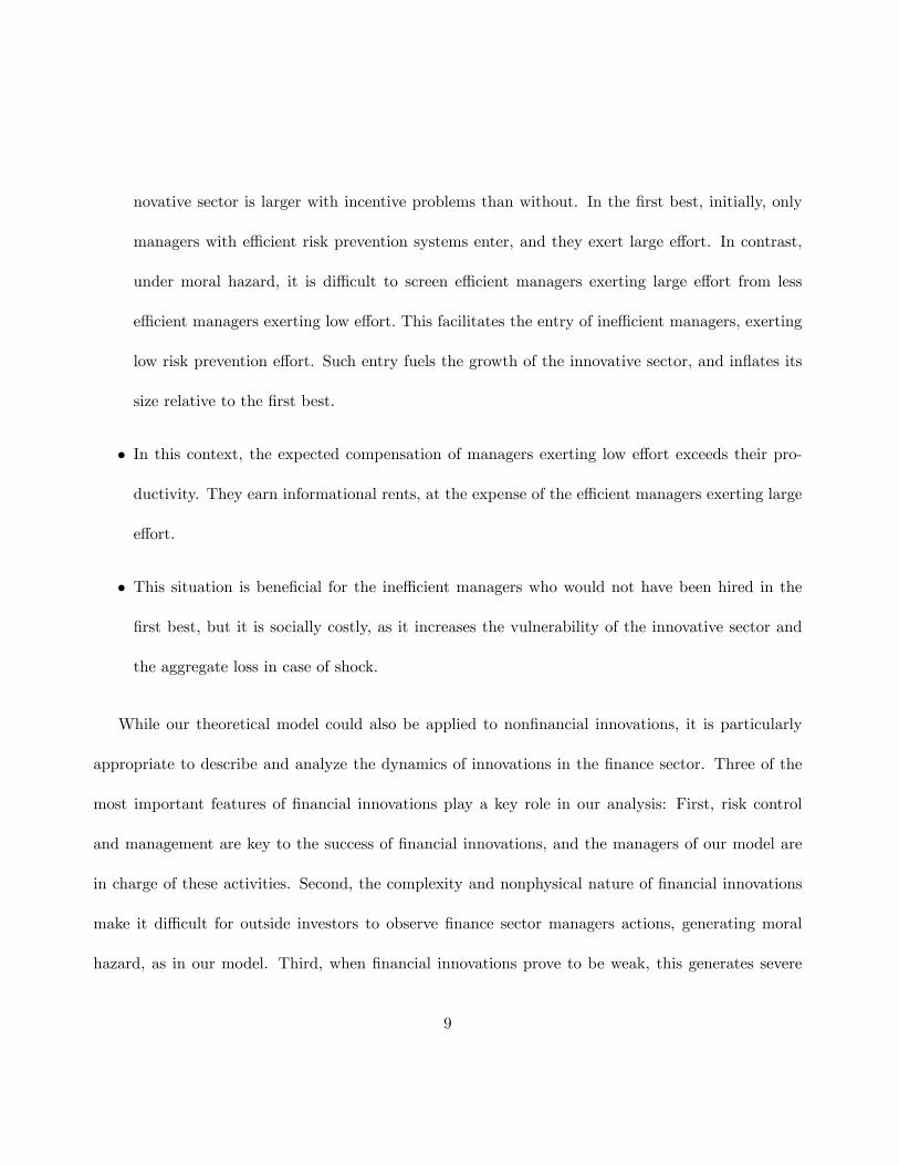
The unfolding of uncertainty in each period t is illustrated in Figure 1. As can be seen in the figure,

when the manager exerts high effort, the project can fail only with probability µθt. Thus, expected

surplus (gross of the managerial cost of effort and the outside opportunity wage) is

αt = (1− µθt)Y − (1 + r). (3)

The larger the probability, θt, that there is a negative shock, the lower the expected surplus αt. We

assume however (to limit the number of cases), that, even when the innovation is known for sure to

be fragile, αt ≥ 0, that is

1− p ≤ 1

µ

Y − (1 + r)

Y. (4)

When the manager exerts low effort, on the other hand, the gross expected surplus is

αt − θt∆Y. (5)

8For example, one can read in the OCC’s Handbook on Large Bank Supervision (2010, 2,3) that “...the OCC assignsexaminers to work full-time at the largest institutions... The OCC’s large bank supervision objectives are designedto...[e]valuate the overall integrity and effectiveness of risk management systems, using periodic validation throughtransaction testing...examiners...attempt to...determine whether...bank systems and processes permit management toadequately identify, measure, monitor, and control existing and prospective levels of risk.”

15

The larger the probability of a shock, the higher the value of risk prevention, θt∆Y . Thus, because αt

is decreasing in θt, αt − θt∆Y , the expected surplus under low effort, is also decreasing in θt. Finally,

we assume that

Cmax > max[(1− µ(1− p))Y − (1 + r),(1− µ(1− p))Y − (1− p)∆Y − (1 + r)

1− e ] (6)

so that, even when the innovation is known for sure to be strong, it is suboptimal to hire the least

effi cient manager. This implies that the mass of managers who could operate effi ciently in the in-

novative sector is lower than the mass of investors, which can be interpreted in terms of scarcity of

managers. Assumption (6) is made for simplicity. Our qualitative results would still obtain under

weaker assumptions.

Throughout the paper, we assume output realizations are observable and contractible. Within

each period t, the sequence of actions is the following:

• investors and managers start with the same belief πt that the innovation is strong,

• investors and managers meet in the labor market,

• managers who have been hired exert high or low effort.

• there is a negative shock or not, and this is observable by all market participants,

• for each project, the investment is successful and yields Y or fails and yields zero.

16

2. Dynamics of Innovative Activities when Effort Is Observable

In this section we consider the case in which efforts (ei) are observable and contractible, so that there

are no incentive problems.

2.1 Equilibrium

Investors and managers meet in the labor market. There are two submarkets: one for managers exert-

ing high effort, the other for managers exerting low effort. A compensation contract is a mapping of

all the observable variables into the compensation of a manager. In the present section, the observable

variables in period t are the state variable θt, the output of the project Y , whether a shock occurred

or not ξt, and the effort of the manager. In the observable effort case, the only thing that matters,

both for the investor and the manager, is the expected compensation of the manager for a given θt

and effort.9

We denote by m the compensation contract for managers hired to exert high effort, and by m the

contract for low effort. For simplicity, we assume market participants are competitive. Thus, they

take the equilibrium contracts as given. The equilibrium condition is that labor supply equals labor

demand. Labor supply in a given submarket is the mass of managers who (weakly) prefer to be hired

in that submarket rather than to not be hired or operate in the other submarket. Labor demand is

the mass of investors who (weakly) prefer to invest in this market rather than to self-invest or operate

in the other market.9 In the next section, we consider the unobservable effort case, in which the precise mapping between observable

variables and compensation matters, because it affects incentives.

17

Market clearing implies

E[m|e, θt] = αt, E[m|e, θt] = max[αt − θt∆Y, 0]. (7)

When αt−θt∆Y ≥ 0, (7) means that investors are indifferent between self-investment, investment with

high effort, and investment with low effort. When αt − θt∆Y < 0, it means investors are indifferent

between self-investment and investment with high effort. To see why (7) is necessary for market

clearing, consider the case in which αt − θt∆Y < 0. In this case suppose we had E[m|e, θt] < αt.

Then all investors would prefer to hire managers to exert high effort, that is, labor demand in the

market for managers exerting high effort would be equal to one. Yet, labor supply could not exceed

F (E[m|e, θt]), which is the mass of managers with cost of effort Ci < E[m|e, θt]. Because this mass

is strictly lower than one (because of (6)), the market would not clear. Thus, when αt − θt∆Y < 0,

market clearing entails E[m|e, θt] = αt as illustrated in Figure 2. Similar arguments apply for the

other cases.

(7) implies that, whenever an investor hires a manager, the latter captures all the surplus generated

by their interaction. This is in line with Berk and Green (2004), where the economic rents flow through

to the managers who create them, not to the investors who invest in them. Our result reflects the

assumption that managers are heterogeneous, and, while the best of them are very good, the worst

ones are quite ineffi cient, as stated in (6). Thus, highly talented managers are scarce. And this matters

because each manager can handle only one project and managers have different Cs.

18

Manager i applies for a job requesting high effort if

E[m|e, θt]− Ci ≥ max[0, E[m|e, θt]− eCi], (8)

whereas she applies for a job requesting low effort if

E[m|e, θt]− eCi ≥ max[0, E[m|e, θt]− Ci]. (9)

Otherwise, she chooses to remain in her initial occupation. Hence manager i choosing between high

effort, low effort, and staying out of the innovative sector obtains the following expected gain

max[E[m|e, θt]− Ci, E[m|e, θt]− eCi, 0]. (10)

Substituting (7) into (10), the expected gain obtained by manager i in the innovative sector is

max[αt − Ci, αt − θt∆Y − eCi, 0]. (11)

Because (11) is also equal to the social value created by the employment of manager i in the innovative

sector, we have that market equilibrium is Pareto optimal. It is natural, because the market is

competitive and frictionless, that the first welfare theorem holds.

19

Denoting

βt =θt∆Y

1− e , γt =αt − θt∆Y

e,

(7), (8), and (9) imply that managers choosing high effort are such that,

Ci ≤ min[αt, βt], (12)

whereas managers choosing low effort are such that10

βt ≤ Ci ≤ γt. (13)

If Ci = αt, agent i is indifferent between effort and staying out of the innovative sector. If Ci = βt,

agent i is indifferent between effort and no effort. If Ci = γt, agent i is indifferent between low effort

and staying out of the innovative sector. Thus, when Ci = αt = βt, we have Ci = γt. Define θ as the

probability of a negative shock such that βt = γt = αt. Simple computations yield

θ =Y − (1 + r)

Y

1

µ+ ∆1−e

. (14)

To focus on the interesting case, we assume that θ is in the support of θ, that is, 1− p < θ < 1− p.

βt increases linearly in θt, whereas γt and αt decrease linearly. These functions are as illustrated in

Figure 3. Inspecting the figure and using conditions (12) and (13), one sees that, for θt > θ, managers

10Note that, as can be seen in Figure 3, when αt < βt, the interval [βt, γt] does not exist.

20

with Ci ≤ αt choose to be employed to exert high effort, whereas managers with Ci > αt prefer to

stay out of the innovative sector. For θt ≤ θ, managers with Ci ≤ βt choose to be employed to exert

high effort, managers with βt ≤ Ci ≤ γt choose to be employed to exert low effort, and managers

with Ci > γt prefer to stay out of the innovative sector. Thus, noting that θt declines as long as the

industry is not hit by a negative shock, we can state our first proposition.

Proposition 1. When θt ≥ θ, all agents hired to manage investment exert high effort, and their

expected compensation, E[m|e, θt] = αt as well as their mass, F (αt), grow as long as the industry is

not hit by a shock.

When θt < θ, while a mass F (βt) of agents exert high effort, a mass F (γt)−F (βt) exert low effort.

The former earn expected compensation, E[m|e, θt] = αt, the latter earn E[m|e, θt] = αt − θt∆Y .

Both expected compensations, and also the mass of managers in the innovative industry, grow as as

long as the industry is not hit by a shock.

When there is a negative shock, compensation and the number of managers working in the innov-

ative industry suddenly drop.

Managers who are more effi cient at controlling risks (with low Ci) are more likely to be employed

in jobs requesting high effort. They correspondingly earn larger compensation. Once confidence has

improved so much that θt becomes lower than θ, the increase in the fraction of managers exerting low

effort tends to push average compensation down. But, controlling for the type of tasks (that is, high

or low effort), compensation continues to grow as long as the innovation is successful.

21

2.2 Inframarginal rents

Inframarginal managers’rents are equal to the difference between their expected compensation and

their cost of effort. Thus, manager i obtains rent equal to

R(Ci, θt) = max[αt − Ci, αt − θt∆Y − eCi, 0]. (15)

By construction, except for the marginal agent, managers employed in the innovative sector earn

strictly positive rents, reflecting the above-mentioned scarcity of highly talented managers. Thus, we

can state the following corollary.

Corollary 1. The expected compensation of managers employed in the innovative sector exceeds

the sum of their cost of effort and their outside opportunity wage. The corresponding infra-marginal

rents (R(Ci, θt)) increase, for all managers, as confidence in the strength of the innovative sector

increases.

The quasirents in Corollary 1 reflect managers’heterogeneity, similarly to Berk and Green (2004).

2.3 Implications of the model with observable effort

2.3.1 Growth and compensation in the innovative sector. As long as there is no negative

shock, confidence in the innovation increases, that is, θt decreases. Proposition 1 implies that this

leads to an increase in the mass of agents hired to manage investments. When θt gets lower than θ, the

innovation is perceived to be so strong that, even with low effort, it can outperform self-investment.

22

This spurs the entry of relatively ineffi cient managers, who are planning to exert low effort. This, in

turn, can induce an increase in the growth of the innovative sector. As long as θt > θ, the size of the

innovative sector is F (αt). Thus, the growth of the innovative sector is given by

dF (αt)

dt=dF (αt)

dθt

dθtdt

= f(αt)dαtdθt

dθtdt

= −f(αt)µYdθtdt

= f(αt)µY |dθtdt|.

As soon as θt < θ, the size of the innovative sector is F (γt). Thus, the growth of the innovative sector

is given by

dF (γt)

dt=dF (γt)

dθt

dθtdt

= f(γt)dγtdθt

dθtdt

= −f(γt)(µ+ ∆)Y

e

dθtdt

= f(γt)(µ+ ∆)Y

e|dθtdt|.

Noting that e < e = 1 and that, at θt = θ, f(αt) = f(γt), we have that the growth of the finance

sector just before θ: dF (αt)dt , is lower than its counterpart just after θ: dF (γt)

dt . Otherwise stated, the

growth of the innovative sector induced by the absence of shock increases when θt hits θ. Graphically,

this corresponds to the fact that, in Figure 3, the absolute value of the slope of γt is larger than that

of the slope of αt.

Thus, noting that confidence increases with the time without negative shocks and also with the

cumulated performance of the innovative sector, which can be empirically measured by cumulated

operating profits, we can state our first implication.

23

Implication 1. The size of the innovative sector is increasing in the length of the period without

negative shock and the cumulative performance of the innovation. After sustained performance, there

is an increase in the growth of the innovative sector.

Because Corollary 1 implies that expected compensation increases with the confidence in the

innovation, we can state the following implication.

Implication 2. The longer the period without negative shock and the larger the cumulative

performance of the innovation, the higher the wage in the innovative sector.

Our theoretical result that compensation in the innovative sector trends upwards is in line with

the empirical findings of Philippon and Resheff (2009).

2.3.2 Deteriorating standards in the innovative sector. When θt > θ, all managers exert

high effort, and after sustained success θt becomes lower than θ, and an increasing fraction of managers

are hired without being requested to exert high effort. Correspondingly, when θt gets below θ, there

is a decline in the proportion of managers exerting large risk prevention effort. More precisely, when

θt < θ the average effort level is

F (βt) +F (γt)− F (βt)

F (γt)e = e+ (1− e)F (βt)

F (γt),

24

which is increasing in θt, because F (βt) is increasing in θt, while F (γt) is decreasing. Thus, as

confidence increases (and θt goes down), there is a decline in the average level of effort requested,

coinciding with a decline in the average effi ciency of risk management systems. Interpreting this as a

decline in risk prevention standards, we obtain the following implication.

Implication 3. After sustained success, there is a decline in risk prevention standards, starting

at the time at which the growth of the innovative sector accelerates.

Implication 3 is consistent with the empirical findings of Dell’Ariccia, Igan and Laeven (2008) who

write in their abstract: “This paper links the current sub-prime mortgage crisis to a decline in lending

standards associated with the rapid expansion of this market.”Dell’Ariccia, Igan and Laeven (2008)

relate their empirical findings to asymmetric information-based theories of financial accelerators (see

Bernanke and Gertler, 1998; Kiyotaki and Moore, 1997). Yet, our analysis shows that agency problems

are not needed to rationalize these findings.11 The decline in standards in implication 3 corresponds

to the entry of financial intermediaries with weaker and weaker risk control systems. To test this

implication, empirical proxies for the strength of risk control systems are needed. One could rely on

the Risk Management Index developed by Ellul and Yerramilli (2010).12

11 In the next section, however, we show that these problems are exacerbated by information asymmetry.12Consistent with our theoretical analysis, Ellul and Yerramilli (2010) find that financial institutions with stronger

risk control systems in 2006 had lower exposure to private—label mortgage—backed securities, had a smaller fraction ofnonperforming loans, and had lower downside risk during the crisis years.

25

2.3.3 Unlikely but large aggregate losses. The probability of a negative shock (θt) decreases

with the number of periods without a shock. For θt ≥ θ, the mass of failing projects in case of a negative

shock is

F (αt)µ.

This decreases with θt, that is, it increases with the confidence in the innovation, simply because,

as confidence grows, more projects are operated in the innovative sector. When θt < θ, the mass of

failures in case of negative shock becomes

F (αt)µ+ [F (γt)− F (αt)]µ+ [F (γt)− F (βt)]∆,

which is also decreasing in θt. This reflects two evolutions: First, as above, as confidence increases,

the number of projects operated in the innovative sector increases. Second, as confidence increases,

an increasing fraction of the projects is operated with low risk prevention effort. Thus, we can state

the next implication.

Implication 4. As the probability of a shock (θt) declines, the size of the loss in case of shocks

increases. After a sustained period of success, when θt gets lower than θ, there is an increase in the

growth of the innovative sector and the mass of failures in case of shock.

Our theoretical analysis thus implies that long-awaited shocks, that come after a period of sus-

tained performance and growing confidence, are more severe than shocks happening during the early

26

developments of the innovation. This is in line with the empirical finding by Dell’Ariccia et al. (2012)

that busts following long booms are worse than busts coming after short booms. The pattern gener-

ated by our model could look like a bubble followed by a crash. Yet it simply reflects how the optimal

level of investment and effort adjusts as agents learn about the strength of the innovation.

2;3.4 The cross-section of failure probabilities. For θt ≥ θ, the failure probability for each

project operated in the innovative sector is θtµ. For θt < θ, the failure probability in the innovative

sector remains equal to θtµ for projects with Ci ≤ βt, but it is θt(µ + ∆) for projects with Ci > βt.

Thus, for θt < θ, the cross-sectional average default rate in the innovative sector is

θt{F (βt)

F (γt)µ+

F (γt)− F (βt)

F (γt)(µ+ ∆)} = θt{µ+ (1− F (βt)

F (γt))∆}.

This is the product of the probability of shock (θt) by the cross-sectional average probability of default

in case of shock. The latter increases with the confidence in the innovative sector.

While for θt ≥ θ, all managers operating in the innovative sector have the same probability of

default: θt∆, for θt < θ, a fraction F (βt)/F (γt) of the managers have default rate in case of shock

equal to µ, while for the others it is µ + ∆. Hence, for θt ≥ θ, the cross-sectional variance of default

probabilities in case of shock is zero, while, for lower values of θt, it is

2F (βt)

F (γt)(1− F (βt)

F (γt))∆2.

27

As θt crosses θ,F (βt)F (γt)

is initially close to one. Then it decreases with further increases in confidence.

Correspondingly, the cross-sectional variance of default probabilities in case of shock is initially very

small, but increases as confidence builds up. On the other hand, if θt decreases enough forF (βt)F (γt)

to

reach one-half, then further increases in confidence reduce this cross-sectional variance. The intuition

is the following. As long as θt > θ, all managers exert high effort, so that there is no cross-sectional

variation in the probability of default in case of shock. When θt crosses θ from above, an initially small

but gradually increasing fraction of managers exerts low effort. Correspondingly, for values of θt below

θ, but not too far from it, heterogeneity in effort exertion across managers increases with confidence.

But, for very low values of θt, the majority of managers exert low effort, and further decreases in θt

increase this majority, thereby reducing the heterogeneity in default probabilities. Correspondingly,

the cross-sectional variance of default probabilities across managers is inverse-U shaped in θt. Our

next implication summarizes this discussion:

Implication 5. As confidence in the innovation improves, the average default rate in case of shock

increases, while the cross-sectional variance of default rates first increases and then decreases.

To test implication 5, one needs empirical proxies for failure probabilities. One could rely on put

options with different strikes, on credit risk implied by interest rates, or on credit default swap prices,

for the market as well as for individual names.

2.3.5 Search for yield and the dynamics of the innovative sector. When r is low, the

return on self-investment is low, leading investors to search for yield. Other things equal, a decrease

28

in r raises αt and θ. This accelerates the entry of managers exerting low effort, and the growth of the

innovative industry, but also increases the size of total losses in case of negative shock. This is stated

in our next implication.

Implication 6. The lower r, the more investors search for yield, the larger the size of the innovative

sector, and the larger the size of total losses in case of shock.

3. Dynamics of Innovative Activities under Moral Hazard

The equilibrium analyzed above corresponds to the perfect market case. In practice, however, in-

novative industries are likely to be plagued with information asymmetries. To shed light on the

consequences of these problems, we now turn to the case in which efforts (ei) are unobservable by

investors.13 We hereafter refer to this situation as moral hazard.

While in the first-best it was suffi cient to consider the expected compensation of managers, under

moral hazard, the precise mapping from observable outcomes to transfers must now be specified.

Because of limited liability of investors, when the realization of Y is zero the compensation of the

manager is also zero. Hence, we need only consider four transfers: m(ξ = 0) when the agent who is

requested to exert high effort is successful and there is no shock, m(ξ = 1) when the agent who is

requested to exert high effort is successful in spite of a shock, and m(ξ = 0) and m(ξ = 1) for the

corresponding outcomes when the agent is requested to exert low effort.13Our modeling of the unobservability of effort is similar to that of Holmstrom and Tirole (1997). In our model,

however, unlike that of Holmstrom and Tirole, i) the consequences of the level of effort depend on whether or not thereis an aggregate shock or not, and ii) the cost of effort is not observable by investors.

29

3.1 Equilibrium

When confidence in the innovation is strong enough, the expected surplus is so large that the first-best

allocation is incentive compatible, in spite of the unobservability of effort. To show this, we exhibit

a contract, m (offered to managers exerting high effort as well as to those exerting low effort) that

implements the first best allocation and is incentive compatible when θt is large enough. This contract

is such that m(ξ = 1) = Y . Because managers receive all the output in case of shock (which is the only

case where effort matters), it is in their own interest to choose the first-best level of effort. Consider,

for example, the incentive compatibility condition for high effort:

E[m|e, θt]− Ci ≥ E[m|e, θt]− eCi, (16)

that is

C ≤ θ∆m(ξ = 1)

1− e . (17)

With m(ξ = 1) = Y , (17) simplifies to

θt∆Y

1− e ≥ Ci,

which is the condition under which, in the first best, a manager entering the innovative sector prefers

to exert high effort rather than low effort. Furthermore, given that m(ξ = 1) = Y , investors break

even if and only if

(1− θt)[Y −m(ξ = 0)] = 1 + r.

30

This is compatible with the limited-liability constraint that m(ξ = 0) ≥ 0 if and only if

θt ≤Y − (1 + r)

Y.

Finally, because investors just break even and managers exert the effi cient level of effort, managers

obtain the entire surplus when they enter the innovative sector. Consequently, it is in their own interest

to make the entry decisions that are first-best optimal. Thus, we can state the following proposition:

Proposition 2. When θt ≤ Y−(1+r)Y , equilibrium is the same with or without moral hazard.

Hereafter, we restrict attention to the more interesting case in which moral hazard matters, that is,

we focus on values of θt aboveY−(1+r)

Y . An important feature of equilibrium dynamics in the first-best

is the switch from the equilibrium regime in which all managers exert effort (arising for θt ≥ θ), to

that in which some exert low effort. Because the choice of effort level is the key decision in our moral

hazard model, it is important to consider the values of θt for which the switch from high to low effort

can occur. Because we focus on θt >Y−(1+r)

Y , this requires that θ > Y−(1+r)Y . This inequality is

equivalent to

1− e > ∆

1− µ, (18)

which we assume hereafter. The interpretation of (18) is the following: The left-hand side is the

additional amount of effort needed to exert large risk prevention. The right-hand side is the relative

31

increase in risk avoided by exerting high effort. Condition (18) states that the cost of switching to

high effort (proportional to left-hand side) is relatively large compared to the benefit (proportional to

the right-hand-side). In that case, the switch from high to low effort occurs relatively early. That is,

θ is relatively large, larger than Y−(1+r)Y .

We now establish, that when θt >Y−(1+r)

Y , under moral hazard, two distinct contracts cannot be

offered in equilibrium. Suppose by contradiction that two distinct contracts are offered, one inducing

high effort, the other low effort.14 As in the first-best (see Equation (7)), market clearing and the

scarcity of managers imply that investors must exactly break even on each contract. Hence, the

expected pay-offs, and the decisions of managers (high effort, low effort, no participation) must be

exactly the same as in proposition 1. Now, proposition 1 implies that there are two active contracts

only when θt < θ, and that contract m (compensating high effort) is chosen by all managers such that

Ci ≤ βt =θt∆Y

1− e . (19)

Similarly to (17), the incentive compatibility condition is

Ci ≤θt∆m(ξ = 1)

1− e (20)

for all the managers i choosing contract m. For the marginal manager (19) holds as an equality and

14We show in the Appendix that one can also rule out situations in which i) one of the two contracts would attractboth managers exerting high effort and managers exerting low effort, or ii) the two contracts would attract managersexerting high effort and managers exerting low effort.

32

(20) can hold only if m(ξ = 1) = Y . As shown above, in the proof of proposition 2, m(ξ = 1) = Y

is compatible with limited liability only when θt ≤ Y−(1+r)Y , which is ruled out by construction. This

shows, by contradiction, that there is always at most one active contract at equilibrium. Hence, we

can state the following proposition:

Proposition 3: Under moral hazard, when (18) holds and θt >Y−(1+r)

Y , at most one contract is

offered at equilibrium.

Our third, striking, result is that, contrarily to the case in which effort is observable, moral hazard

implies that there is always a positive fraction of active managers that exert low effort at equilibrium.

Again, the proof proceeds by contradiction. Suppose all active managers would exert high effort. Then

equilibrium would involves a unique contract, m. m should be such that investors would at least break

even, that is,

(1− θt)m(ξ = 0) + θt(1− µ)m(ξ = 1) ≤ (1− θtµ))Y − (1 + r) ≡ αt. (21)

Because manager’s limited liability implies m(ξ = 0) ≥ 0, (21) implies

m(ξ = 1) ≤ αtθt(1− µ)

.

Consequently,

θt∆m(ξ = 1) ≤ αt∆

(1− µ)< αt(1− e),

33

where the second inequality stems from (18). Thus, the marginal manager, with cost of effort Ci = αt,

would strictly prefer to exert low effort, which establishes the contradiction. We can thus state the

following proposition.

Proposition 4. Under moral hazard, when (18) holds and θt >Y−(1+r)

Y , there is always a positive

fraction of active managers that exert low effort at equilibrium.

We now characterize the equilibrium arising in that case. We know that it must be a pooling

equilibrium, in which only one contract, m, is offered and some of the managers accepting it exert

high effort, while others exert low effort. Denoting

C =θt∆m(ξ = 1)

1− e , (22)

and

C =(1− θt)m(ξ = 0) + θt(1− µ−∆)m(ξ = 1)

e, (23)

the managers who prefer high effort than low effort are those with Ci ≤ C, while those who prefer to

be hired and exert low effort are such that C ≤ Ci ≤ C.

The market clearing condition, requiring that investors earn zero profit, is

(1− θt)m(ξ = 0) + θt(1− µ−∆x)m(ξ = 1) = (1− θt(µ+ ∆x))Y − (1 + r), (24)

34

where x is the fraction of the managers hired in the innovative sector who exert low effort, that is,

x = 1− F (C)

F (C)= 1−

F ( θt∆m(ξ=1)1−e )

F ( (1−θt)m(ξ=0)+θt(1−µ−∆)m(ξ=1)e )

.

A contract such that m(ξ = 0) > 0 cannot be an equilibrium. Indeed an investor could undercut

this contract by offering another one with a lower m(ξ = 0) and a larger m(ξ = 1), in such a way

that the expected gain for a manager exerting low effort would be the same (leaving C unchanged)

while increasing the gain from high effort (thus raising C).15 This would attract exactly the same

managers, but a higher fraction of them would make an effort, thus generating positive expected gains

for the investors. Hence, in equilibrium, we must have

m(ξ = 0) = 0. (25)

Thus, x rewrites as

x = 1−F ( θt∆m(ξ=1)

1−e )

F ( θt(1−µ−∆)m(ξ=1)e )

.

For simplicity, we hereafter assume costs are uniformly distributed over [0, Cmax].16 Then the

15 It is indeed possible to increase m(ξ = 1) because it is less than Y . To see this, consider the market clearingcondition, which implies, when m(ξ = 0) > 0, that m(ξ = 1) < [(1− θt(µ+ ∆x))Y − (1 + r))](θt(1− µ−∆x))−1, whichis decreasing in θt. Now, proposition 4 assumes θt > (Y − (1 + r))/Y , thus m(ξ = 1) is lower than [Y − (µ+ ∆x)(Y −(1 + r))− (1 + r)]((1− µ−∆x)Y−(1+r)

Y)−1 which simplifies to Y .

16The result that x is a constant obtains whenever f(m), which can be interpreted as labor supply, has constantelasticity. More generally, if elasticity is nondecreasing, the equilibrium is unique and exhibits the additional propertythat x increases with the confidence in the innovation.

35

fraction of managers exerting low effort simplifies to

x = 1− e

1− e∆

1− µ−∆. (26)

The condition under which m(ξ = 1) is nonnegative is

[1− θt(µ+ x∆)]Y − (1 + r) ≥ 0, (27)

which simplifies to

θt ≤1

µ+ x∆

Y − (1 + r)

Y, (28)

If (28) does not hold, there is a market breakdown and no manager is hired in the innovative sector.

Otherwise, m(ξ = 1) is nonnegative and is obtained by substituting m(ξ = 0) = 0 and (26) into (24)

m(ξ = 1) =(1− θt(µ+ ∆x))Y − (1 + r)

θt(1− µ−∆x). (29)

Substituting (26), (25), and (29) into (23), we have

C =1− µ−∆

1− µ−∆[1− e

1−e∆

1−µ−∆

] (1− θt(µ+ ∆x))Y − (1 + r)

e, (30)

which is linear and decreasing in θt. The above analysis leads to our next proposition, illustrated in

Figure 4.

36

Proposition 5: Under moral hazard, when (18) hold and costs are uniformly distributed over

[0, Cmax], equilibrium is as follows.

When

θt >1

µ+ x∆

Y − (1 + r)

Y, (31)

no manager is hired in the innovative sector.

When

1

µ+ x∆

Y − (1 + r)

Y≥ θt >

Y − (1 + r)

Y,

there exists a pooling equilibrium, in which only one contractm is offered, a fraction x of the managers

working in the innovative sector exerts low effort, and the complementary fraction exerts high effort.

The average expected compensation of managers is given by the left-hand side of (27), which increases

as confidence in the innovative sector improves.

The intuition underlying the proposition is the following:

When the risk of a negative shock is so high that (31) holds, incentive problems generate an

“innovation trap.”If effort was observable, it would be feasible to request high effort from all managers.

This would enable investment to take place, which would, in turn, generate learning about the strength

of the innovation. Because of moral hazard however, when the risk of a negative shock is high it is

impossible to ensure that all managers exert high-effort, therefore investment in the innovative sector

is not profitable. So the innovation cannot develop, and learning cannot take place.

When θt is intermediate, while in the first-best managers exerting low effort and managers exerting

37

high effort would choose different contracts, under asymmetric information such sorting is not incentive

compatible. Hence, there is pooling. In line with the argument that led to proposition 3, this pooling

equilibrium cannot be undercut by raising managers’ success payments and reducing their failure

payments so as to attract only good managers (the traditional cream-skimming argument) because

failure payments are zero and negative payments are precluded by managers’limited liability.

3.2 Implications of incentive constraints

The next implication summarizes how moral hazard affects the development of innovations. In line

with the above analysis, we focus on the case in which θt is large and (18) holds. The first part of

proposition 5 implies that when initial confidence is very low, as θ0 >1

µ+x∆Y−(1+r)

Y , and (18) holds,

moral hazard precludes the development of innovations that would have occurred in the first best.

This yields the following implication.

Implication 7. When θ0 >1

µ+x∆Y−(1+r)

Y a decline in the rate of return on standard investments

(r) can trigger a wave of innovations.

When r declines, the threshold level above which innovations are trapped goes up. Hence, inno-

vations that had become available but had not been able to develop can suddenly get implemented.

Thus, there is a wave of innovations.

Now turn to the second part of proposition 4 and its illustration in Figure 4. Comparing the slopes

of the lines in Figure 4, and reasoning as for implication 1, we see that when effort is unobservable

38

and θ ∈ [θ, Y−(1+r)(µ+∆x)Y ], the rate of growth of the innovative sector is larger than in the first best. This

reflects that many managers enter and exert low effort, in contrast with the first best where only

effi cient managers, exerting high effort, would enter.

That moral hazard spurs the entry of ineffi cient managers can lead to a situation in which the size

of the innovative sector is larger than in the first best.17 To see how this obtains, consider Figure 4.

Managers that are hired and exert low effort are those with Ci in [C, C]. As illustrated in Figure 4,

the C line intersects the horizontal axis at θt = 1µ+x∆

Y−(1+r)Y , which is larger than the point at which

γt intersects the horizontal axis, θt = 1µ+∆

Y−(1+r)Y , but lower than the point at which αt intersects the

horizontal axis. On the other hand, C intersects γt for θt = Y−(1+r)Y , a point at which γt > αt. Hence,

there exists a threshold θ∗ ∈ [Y−(1+r)Y , 1

µ+x∆Y−(1+r)

Y ), such that C > max[αt, γt] for θt ∈ [Y−(1+r)Y , θ∗).

Now, in this region, the size of the innovative sector in the first best is F (max[αt, γt]), while in the

second best it is F (C). Hence, for these values of θt, the size of the innovative sector is larger under

moral hazard than in the first best. The next implication summarizes the above discussion.

Implication 8. Under moral hazard, when (18) holds, if the innovation is not trapped, the

growth rate of the innovative sector is strictly larger than in the first best, as long as θt > θ. Further-

more, there exists a threshold θ∗ ∈ [Y−(1+r)Y , 1

µ+x∆Y−(1+r)

Y ), such that, for θt ∈ [Y−(1+r)Y , θ∗), the size

of the innovative sector is larger than in the first best.

The intuitive economic reason why moral hazard inflates the innovative sector is that, as mentioned

17This is reminiscent of the overinvestment result of De Meza and Webb (1987).

39

above, it spurs the entry of managers exerting low effort. This fuels the growth of the sector. On the

other hand, it lowers the average expected surplus generated by investments in the innovative sector.

One could think this decline in expected surplus would deter investment by principals. This is not

the case because, in the pooling equilibrium of proposition 4, there is cross-subsidization of managers

exerting low effort by managers exerting high effort. The former receive higher expected compensation

than the (negative) surplus they generate for society; that is, they earn rents. In contrast, the managers

exerting high effort receive lower expected compensation than the (positive) surplus they generate for

society. Hence, the expected losses incurred by investors hiring managers who turn out to exert low

effort are offset by their expected gains when hiring managers who turn out exerting high effort. Thus,

in a sense, the excessively inflated growth of the innovative sector is funded by the subsidies of the

managers exerting high effort. And these subsidies result in agency rents for managers exerting low

effort, as stated in the next implication.

Implication 9. Under moral hazard, when (18) holds, for θt ∈ [Y−(1+r)Y , θ∗), agents exerting low

effort earn agency rents.

Taken together, implications 8 and 9 contrast with previous theoretical results. To the extent

that rents are transfers from principals to agents, they tend to deter investment by managers. In

this context, moral hazard reduces the size of the sector relative to the first best, as, for example, in

Axelson and Bond (2011). This is not the case in the present model, where, in contrast with Axelson

and Bond (2011), not only effort but also the cost of effort are unobservable. In this context, the rents

40

earned by ineffi cient agents are funded by the effi cient agents, rather than the principals.

While the inflated growth of the innovative sector is privately optimal for the managers exerting

low effort, who would not have been hired in the first best, it is socially costly: it drives expected

utilitarian welfare below its first-best level, due to the value-destroying entry of managers exerting low

effort. This social cost materializes when a negative shock hits and large losses are incurred due to

lack of risk prevention by low-effort managers. This is stated in the next implication.

Implication 10. Under moral hazard, when (18) holds, for θ ∈ [Y−(1+r)Y , θ∗), default probabil-

ities and aggregate losses in case of shock are higher than in the first best.

4. Conclusion

Our analysis of the dynamics of innovations and risk under learning yields two key insights: First, the

strongest growth episodes of the innovative sector are fueled by the entry of managers exerting low

risk prevention effort - and therefore correspond to a decline in risk prevention standards. Second,

under moral hazard, there is excessive entry of managers exerting low effort and earning informational

rents, so that the innovative sector is larger and riskier than in the first best.

Thus, in our model, the signature of moral hazard is strong growth at early stages of the develop-

ment of the innovation. In the first best, early growth is slow, because limited confidence implies only

managers exerting high effort should enter. Under asymmetric information, early growth is strong, in

41

spite of limited confidence, due to the entry of managers exerting low prevention efforts, that cannot

be screened from those exerting high prevention effort.

While the present model features only managers and investors, it would be interesting to extend the

analysis by introducing a supervisor or regulator, better able than investors to monitor the managers’

risk management systems. Because under asymmetric information there is excess entry of managers

with ineffi cient risk management systems, supervisory monitoring could improve welfare by imposing

compliance to risk management standards. When should that occur? Our theoretical analysis suggests

that strong growth should not be taken as an encouraging sign that the innovation is healthy, calling

for “light-touch regulation.”Quite to the contrary, it is in periods of strong growth that resources

should be spent to monitor the innovative sector, check risk prevention standards, and bar entry for

institutions with weak risk management systems.

Also, while our results obtain with rational agents, they could be amplified by psychological bi-

ases, such as, e.g., overconfidence. After a few years without negative shocks, overconfident market

participants would become excessively confident that the innovation is strong.18 This would magnify

the effects we analyze, reduce risk prevention further, and make the innovative sector more vulnerable.

18This is consistent with the approach taken by Daniel, Hirshleifer, and Subrahmanyam (1998) or Gervais and Odean(2001). In their models, however, agents overestimate the precision of private signals, whereas here they would overesti-mate the precision of public signals.

42

References

Atkeson, A., A. Eisfeldt, and P.O. Weill. 2013. The market for OTC derivatives. Working Paper,

UCLA.

Axelson, U., and P. Bond. 2011. Wall Street occupations: An equilibrium theory of overpaid jobs.

Working Paper, University of Minnesota & LSE.

Barbarino, A., and B. Jovanovic. 2007. Shakeouts and market crashes. International Economic

Review 48:385-420.

Bergemann, D., and U. Hege. 1998. Dynamic Venture Capital Financing, Learning and Moral

Hazard. Journal of Banking and Finance 22:703-35.

– – – – – – – – – – – . 2005. The financing of innovation: learning and stopping. Rand Journal

of Economics 36:719-52.

Berk, J., and R. Green. 2004. Mutual fund flows and performance in rational markets. Journal of

Political Economy 112:1269-95.

Bernanke, B., and M. Gertler. 1989. Agency costs, net worth and business fluctuations. American

Economic Review 79:14-31.

Bikhchandani, S., D. Hirshleifer, and I. Welch. 1992. A theory of fads, fashion, custom and cultural

change as informational cascades. Journal of Political Economy 100:992-1026.

Bolton, P., and C. Harris. 1999. Strategic experimentation. Econometrica 67:349-74.

Bolton, P., T. Santos, and J, Scheinkman. 2013. Cream skimming in financial markets. Working

43

Paper, Columbia University.

Caballero, R., and A. Krishnamurthy. 2008. Collective risk management in a flight to quality

episode. Journal of Finance 63:2195-236.

Comptroller of the Currency - Administrator of National Banks. 2010. Large Bank Supervision -

Comptroller.s Handbook.

Daniel, K., D. Hirshleifer, and A. Subrahmanyam. Psychology and security market under- and

over-reactions. Journal of Finance 53:1839-85.

Daniel, K., R. Jagannathan, and S. Kim. 2012. Tail risk in momentum strategy returns. Working

Paper, Columbia University.

Daniel, K., and T. Moskowitz. 2012. Momentum crashes. Working Paper, Columbia University.

Dell’Ariccia, G., D. Igan, and L. Laeven. 2008. Credit booms and lending Standards: Evidence

from the subprime mortgage market. IMF Working Paper, WP/08/106

Dell’Ariccia, G., D. Igan, L. Laeven, H. Tong, B. Bakker, and J. Vandenbussche. 2012. Policies

for macrofinancial stability: How to deal with credit booms. IMF Staff Discussion Note SDN/12/06

DeMarzo, P., and Y. Sannikov. 2008. Learning in dynamic incentive contracts. Working Paper,

Stanford University.

De Meza, D., and D. Webb. 1987. Too much investment: A problem of asymmetric information.

Quarterly Journal of Economics 102:281-92

Diamond, D. 1991. Monitoring and reputation: The choice between bank loans and directly placed

debt. Journal of Political Economy 99:689-721.

44

Ellul, A., and V. Yerramilli. 2010. Stronger risk controls, lower risk: Evidence from U.S. bank

holding-companies. Working Paper, Kelley School of Business, Indiana University.

Gervais, S., and T. Odean. 2001. Learning to be overconfident. Review of Financial Studies

14:1-27.

Holmstrom, B., 1979. Moral hazard and observability. Bell Journal of Economics 10:74-91.

Holmstrom, B., and J. Tirole. 1997. Financial intermediation, loanable funds, and the real sector.

Quarterly Journal of Economics 112:663-91.

Kiyotaki, N. and J. Moore. 1997. Credit cycles. Journal of Political Economy 105:211-48.

Pastor, L., and P. Veronesi. 2006. Was there a Nasdaq bubble in the late 1990’s ?. Journal of

Financial Economics 81:61-100.

Persons, J., and V. Warther. 1997. Boom and bust patterns in the adoption of financial innova-

tions. Review of Financial Studies 10:939-67.

Philippon, T., and A. Resheff. 2008. Wages and human capital in the U.S. financial industry:

1909-2006. Working Paper, New York University.

Noe, T., and M. Rebello. Forthcoming. To each according to her luck and power: Optimal

corporate governance and compensation policy in a dynamic world. Review of Financial Studies.

Rob, R. 1991. Learning and capacity expansion under demand uncertainty. Review of Economic

Studies 58:655-77.

Rogers, E. M. 1962. Diffusion of innovations. Glencoe: Free Press.

Zeira, J. 1987. Investment as a process of search. Journal of Political Economy 95:204-10.

45

– – – . 1999. Informational overshooting, booms and crashes. Journal of Monetary Economics

43:237-57.

46

Appendix. Complement to the Proof of Proposition 3

In the text we showed that, when θ > [Y − (1 + r)] /Y,there cannot be two contracts in equilibrium,

one inducing high effort only, and the other inducing low effort only. We now show that the proof

extends to rule out the situation in which one of the two contracts would attract both managers

exerting high effort and managers exerting low effort.

The proof proceeds by contradiction. Suppose there were two contracts:

• mboth, inducing low effort by a fraction x of the managers who choose it and high effort by the

remaining fraction,

• and mhigh, inducing only high effort.

If one of these two contracts gave higher compensation for high effort than the other, then all

managers exerting high effort would choose the former, and the latter would not attract any manager.

Thus, for both contracts to attract managers exerting high effort, it must be that they give managers

the same expected pay-off conditionally on e = 1; that is,

(1− θ)mboth(ξ = 0) + θ(1− µ)mboth(ξ = 1) = (1− θ)mhigh(ξ = 0) + θ(1− µ)mhigh(ξ = 1).

Moreover competition between investors implies they exactly breakeven for each of the two con-

47

tracts; that is,

(1− θ)mhigh(ξ = 0) + θ(1− µ)mhigh(ξ = 1) = (1− θµ)Y − (1 + r),

and

(1− θ)mboth(ξ = 0) + θ(1− µ−∆x)mboth(ξ = 1) = (1− θµ− θ∆x)Y − (1 + r).

Equality of expected transfers conditional on high effort along with the breakeven condition for mhigh

imply

(1− θ)mboth(ξ = 0) + θ(1− µ)mboth(ξ = 1) = (1− θµ)Y − (1 + r).

Substracting from the breakeven condition for mboth, this yields mboth(ξ = 1) = Y . Substituting

mboth(ξ = 1) = Y into the breakeven condition for mboth, we have

mboth(ξ = 0) = Y − 1 + r

1− θ ,

which contradicts the limited liability condition that mboth(ξ = 0) ≥ 0 when θ > [Y − (1 + r)]/Y .

Thus, when θ > (Y − (1 + r))/Y , it cannot be the case, in equilibrium, that one contract attracts

only managers exerting high effort, whereas the other attracts both managers exerting high effort

and managers exerting low effort. Reasoning along similar lines, one rules out the case in which one

contract attracts managers exerting low effort only, whereas the other attracts managers exerting high

effort, as well as managers exerting low effort.

48

Finally, we rule out the possibility that there would be two different contracts, m1 and m2, each

attracting both managers exerting high effort and managers exerting low effort. For both contracts to

attract managers exerting high effort,

(1− θ)m1(ξ = 0) + θ(1− µ)m1(ξ = 1) = (1− θ)m2(ξ = 0) + θ(1− µ)m2(ξ = 1).

For both contracts to attract managers exerting low effort,

(1− θ)m1(ξ = 0) + θ(1− µ−∆)m1(ξ = 1) = (1− θ)m2(ξ = 0) + θ(1− µ−∆)m2(ξ = 1).

Substracting the latter equality from the former, we get m1(ξ = 1) = m2(ξ = 1). Substituting, we get

m1(ξ = 0) = m2(ξ = 0). Hence, we cannot have two different contracts.

49

Figure 1. The structure of uncertainty in period t

Invest

Innovation is strongθ =1

Innovationis weakθ =0

πt

1− πt

0

μ + (1-e)Δ

No shock

Shock

p

p

Default probability

0

μ + (1-e)Δ

No shock

Shock

1- p

1- p

Figure 2. Market clearing when αt < θ Δ Y

αtE(m|e,θt)

1

Demand for managers exerting large effort

Supply of managers exerting large effort

F(E(m|e,θt))

θtθ

γ

Ci

Figure 3. Equilibrium dynamics without incentive problems

β

α is the expected surplus generated with large effort (gross of the cost of effort).β is the threshold value of C, below which large effort is preferred to low effort.γ is the threshold value of C, below which delegated investment with low effort ismore valuable than self-investment. When Ci < min[α,β], there is large effort. When β < Ci < γ , there is low effort.

^

α

θt

γCi

Figure 4. Equilibrium under moral hazard when Δ/(1-μ) < 1 – e

α, β, and γ are as in Figure 3. For θ > (Y –(1+r)/Y, when Ci < C, there is large effort. When C < Ci < C, there is low effort. For θ < (Y –(1+r)/Y, when Ci < β, there is large effort, and when β < Ci < γ , there is low effort.

β

Y – (1+r) θ Y – (1+r) θ∗ Y – (1+r) Y (μ+Δ)Y (μ+Δ x)Y

α

^

C

C