Embed Size (px)
Citation preview

Dynamics of Flexible Solar Updraft Towers
by
Michael Chi
A thesis submitted in partial fulfillment of the requirements for the degree of
Master of Science
in
Applied Mathematics
Department of Mathematical and Statistical Sciences
University of Alberta
© Michael Chi, 2014

Abstract
Solar updraft towers offers a simple and alternative method of generating
electricity. However, it is unclear on how to build a tall, free standing structure
that can withstand the unpredictable and destructive force of the wind. A
tower consisting of stacked inflatable toroidal elements have been suggested
and the dynamics of the tower will be analyzed. Using Lagrangian reduction
by symmetry, the theory for the 3D motion for the tower is developed. By
confining the motion to two-dimensions, numerical simulations are performed
to study the tower’s stability and is compared with the data collected from a
experimental prototype showing good agreement with theoretical results.
ii

Preface
Research of the thesis in Chapters 2-4 has been performed in collaboration
with Dr. V Putkaradze from the University of Alberta, and Dr. F Gay-Balmaz
from Ecole Normale Superieure de Paris. Experimental data in Chapter 5
was collected by Dr. P Vorobieff. Chapters 2-5 have been submitted for
publication. My work includes verifying the equations in Chapters 2-4 and
computation of some numerical simulations in Chapter 5.
iii

Acknowledgements
First, I would like to express my deep gratitude to Dr. Vakhtang Putkaradze
for his support and guidance in my research. His helpful suggestions and advice
has helped me enormously in writing my thesis. It has been a great pleasure
to work under his supervision.
I would also like to thank my fellow colleagues Patrick Conner and Travis
Boblin for their support throughout my graduate studies. It has been a tough,
yet exciting experience but their encouragement has kept me going and I am
truly grateful for such wonderful friends.
Lastly, I would like to thank all the students and professors that made an
impact in my graduate career at the University of Alberta. All the lasting
memories will be cherished forever.
iv

Table of Contents
1 Introduction 1
1.A Free rigid rotation . . . . . . . . . . . . . . . . . . . . . . . . . 3
1.B The principle of stationary action . . . . . . . . . . . . . . . . 6
2 Methods of Geometric Mechanics 10
2.A Setup of the dynamical equations . . . . . . . . . . . . . . . . 10
2.B Derivation of the equations of motion . . . . . . . . . . . . . . 17
3 Two-Dimensional Dynamics 25
4 Numerical Simulations 28
5 Experiments 31
6 Conclusion 35
Bibliography 37
A Numerical codes (MATLAB) 38
v

List of Tables
5.1 Horizontal deflection of tower top vs. wind speed. . . . . . . . 33
vi

List of Figures
1.1 Schematic diagram of solar updraft tower with chimney. . . . 3
2.1 Setup of the system and explanation of variables used in the
paper. . . . . . . . . . . . . . . . . . . . . . . . . . . . . . . . 11
4.1 Snapshots of dynamics with 20 tori and parameters outlined as
above. All sizes are in m. . . . . . . . . . . . . . . . . . . . . 30
5.1 Photographs of UNM solar chimney prototype: a) wind speed
0.7 m/s from the south (left) and overall view, b) wind speed
2.2 m/s, c) wind speed 20.1 m/s. The overpressure in the tori
is uniform at 0.17 atm. . . . . . . . . . . . . . . . . . . . . . 32
5.2 Left: steady deflection angles computed from (3.7). Notice al-
most linear dependence of φk on the height. Right: comparison
of the shape given by a convergent steady state of (3.7) with
experiments for 2.2 m/s wind speed. . . . . . . . . . . . . . . 33
vii

Chapter 1
Introduction
Solar updraft towers provide an alternative for generating electricity from so-
lar radiation. The main idea behind the production of energy is quite simple.
The air within a collector (greenhouse) is heated from solar radiation. The
warmer air then escapes through a tall pipe which connects the hot volume
of the collector with the cooler air above the ground. The temperature differ-
ence induces convection which turns a turbine within the pipe and generates
electricity. As a comparison to the traditional photovoltaic (PV) cells, one
advantage of the solar towers is the operation of the tower during both the
day and the night. The continual temperature difference between the col-
lector and the pipe due to the thermal mass beneath the ground allows the
tower to operate whereas the PV cells are only optimal during the peak of
the day. Another advantage over most conventional power stations, such as
coal or nuclear power plants, is that the solar towers do not require cooling
water. This is especially beneficial for countries where the water supply is
demanding. Although the concepts and ideas behind solar towers seem quite
feasible, it is important to consider both the costs to build and maintain the
1

towers as well as the efficiency. One of the ways to improve the efficiency is
to increase the temperature differential between the greenhouse on the bot-
tom and the exhaust at the top. This can be achieved by building a taller
tower, however, this would increase the material costs to construct the tower
and maintenance can be challenging for a larger tower. These factors must be
taken into consideration when designing the most economically cost-effective
tower.
The first operational prototype [Haaf et al. 1983] was built in Manzanares,
Spain, in 1982 and the tower was constructed with thin iron sheets. The tower
had operated for approximately eight years, but unfortunately, the tower had
collapsed and was decommissioned in 1989 [Mills 2004] because the tower’s
guy-wires were not protected against corrosion and had failed due to rust and
storm winds. To circumvent this issue, a different approach to building a rigid
tower has been suggested by authors [Putkaradze et al. 2013] who proposed
constructing the tower out of stacked inflatable tori. The shape of the tower
would be such that the deformation due to wind loading is spread uniformly
along the tower. There are several advantages of making an inflatable tower.
One would be the potential to reducing the overall costs to erect and maintain
a tall tower. The tower can be deflated and re-inflated for repairs and for
situations such as severe weather conditions. Damages to the tower can be
avoided quite easily and will substantially lower the costs for repairs. The
inflatable tori can be pressurized individually by using remote pumps. It is
interesting to consider the dynamics of the inflatable tower and whether or
not the tower can withstand fierce winds.
The main focus of the dissertation is to analyze the dynamics of the in-
flatable tower and to study the tower’s stability. The motion of the tower can
2

Figure 1.1: Schematic diagram of solar updraft tower with chimney.
be seen as a rigid body undergoing rotations, although it’s not quite exactly a
rigid body since the toroidal elements can be deformed from the compression
of adjacent tori. The methods of geometric mechanics will be helpful to de-
termine geometrically exact equations for the motion of the tower. Free rigid
motion and principles from Lagrangian mechanics will be briefly stated before
deriving the equations for the tower.
1.A Free rigid rotation
In free rigid rotation [Holm 2008], a body rotates about its centre of mass and
the pairwise distances between all points in the body remain fixed. A system of
coordinates in free rigid motion is stationary in a rotating orthonormal basis.
3

This rotating orthonormal basis is given by
ei(t) = Λ(t)Ei(0) , i = 1, 2, 3, (1.1)
where Λ(t) is an orthogonal 3× 3 matrix, Λ−1 = ΛT .
The unit vectors Ei(0), i = 1, 2, 3 denote an orthonormal basis for fixed
reference coordinates. Every point r(t) in rigid motion may be written in
either coordinate basis as
r(t) = rj0(t)Ej(0), (1.2)
= riei(t), (1.3)
where the components ri satisfy ri = δijr
j0(0) for the choice that the two bases
are initially aligned.
Using the orthogonality of Λ(t), that is Λ(t)ΛT (t) = Id, we may differenti-
ate this equation with respect to time to obtain
0 =d
dt
�Λ(t)ΛT (t)
�=
·Λ(t)ΛT (t) + Λ(t)
·Λ
T
(t)
=·Λ(t)ΛT (t) +
�·Λ(t)ΛT (t)
�T
=·Λ(t)Λ−1(t) +
�·Λ(t)Λ−1(t)
�T
= ω + ωT
where ω :=·Λ(t)Λ−1(t). From the above computation, it follows that the
matrix ω is skew-symmetric which allows one to introduce the corresponding
angular velocity vector ω(t) ∈ R3. The components ωk(t) of the angular
4

velocity vector, with k = 1, 2, 3, are given by
ωij(t) = −�ijkωk(t) , (1.4)
where �ijk is the anti-symmetric tensor.
Equation (1.4) defines the hat map, and one may write the matrix compo-
nents of ω in terms of the components of ω as
ω =
0 −ω3 ω2
ω3 0 −ω1
−ω2 ω1 0
. (1.5)
The velocity in space of a point at r is found by
·r(t) = ri ·
ei(t) = ri·Λ(t)ei(0) (1.6)
= ri·Λ(t)Λ−1(t)Λ(t)ei(0) (1.7)
= riωei(t) (1.8)
= ωr(t) (1.9)
= ω × r(t) . (1.10)
Thus, the velocity of free rigid motion of a point displaced by r from the centre
of mass is a rotation in space of r about the time-dependent angular velocity
vector ω(t).
Remark (Notation): In (1.10), the notation ω ∈ so(3) is used for the anti-
symmetric matrix corresponding to the vector ω ∈ R3. Throughout the rest
of the dissertation, vectors in R3 will be denoted by bold symbols v ∈ R3
5

and their corresponding antisymmetric matrix will be denoted by regular
symbols v ∈ so(3). They verify the relation v = �v, where the hat map
v ∈ R3 �→ �v ∈ so(3) is the Lie algebra isomorphism defined by �vx = v× x,
for all x ∈ R3.
1.B The principle of stationary action
In Lagrangian mechanics, a mechanical system in a configuration space with
generalised coordinates and velocities, qi,·q
i, i = 1, 2, . . . , 3N, is characterised
by its Lagrangian defined as
L(q,·q) := K(q,
·q)− U(q), (1.11)
where K(q,·q) is the kinetic energy and U(q) is the potential energy of the
system. The motion of a Lagrangian system is determined by the principle of
stationary action, formulated using the operation of variational derivative.
The variational derivative of a functional S[q] is defined as its linearisation
in an arbitrary direction δq in the configuration space. That is, S[q] is defined
as
δS[q] := limε→0
S[q + εδq]− S[q]
ε=
d
dε
���ε=0
S[q + εδq] =:
�δS
δq, δq
�, (1.12)
where the pairing �·, ·� is obtained in the process of linearisation.
The Euler-Lagrange equations,
[L]qi :=d
dt
∂L
∂·q
i −∂L
∂qi= 0 , (1.13)
6

follows from stationarity of the action integral, S, defined as the integral over
a time interval t ∈ (t1, t2),
S =
� t2
t1
L(q,·q)dt. (1.14)
Then the principle of stationary action, also known as Hamilton’s principle,
δS = 0 (1.15)
implies [L]qi = 0, for variations δqi that vanish at the endpoints of time.
To demonstrate the methods of geometric mechanics, which will be used
later on more complex systems, let us apply the principle to the Lagrangian
L(ω) =1
2Iω · ω, (1.16)
where K(ω) = 12Iω · ω is the kinetic energy of a rigid body and �ω := Λ−1
·Λ ∈
so(3) is the anti-symmetric matrix corresponding to the angular velocity vector
ω. The variation δω induced by the variation δΛ is computed as follows:
δ�ω = δ(Λ−1·Λ) = δ(Λ−1)
·Λ + Λ−1δ
·Λ
= −Λ−1δΛΛ−1·Λ +
·Σ + ωΣ
=·�Σ + ωΣ− Σω
=·�Σ + �ω ×Σ
where Σ := Λ−1δΛ ∈ so(3) is an arbitrary curve satisfying Σ(0) = Σ(T ) = 0.
7

The second line of the calculation uses the relation
·Σ = −Λ−1
·ΛΛ−1δΛ + Λ−1δ
·Λ = −ωΣ + Λ−1δ
·Λ.
The last line uses the commutator of two anti-symmetric matrices which cor-
responds to the cross product of their corresponding angular velocity vectors,
i.e. [ω, Σ] := ωΣ− Σω = �ω ×Σ. Thus we obtain
δω =·Σ−Σ× ω.
Using Hamilton’s principle of stationary action gives
δ
� T
0
L(ω)dt =
� T
0
δL
δω· δωdt = 0.
Integration by parts yields
� T
0
δL
δω· δωdt =
� T
0
δL
δω·�
·Σ−Σ× ω
�dt
=
� T
0
�− d
dt
�δL
δω
�· Σ− ω × δL
δω· Σ
�dt +
δL
δω· Σ
���T
0
= −� T
0
�d
dt+ ω×
�δL
δω· Σdt.
Since Σ is arbitrary, it follows that
�d
dt+ ω×
�δL
δω= 0 .
It is straightforward to see that
δL
δω= Iω,
8

and thus the equations of motion are given by
d
dt(Iω) = Iω × ω.
which is indeed the equation for rigid body motion.
9

Chapter 2
Methods of Geometric
Mechanics
2.A Setup of the dynamical equations
Let us consider a flexible tower consisting of N toroidal elements with inner
radius dn and outer radius qn, n = 1, . . . , N , as shown in Fig. 2.1. In practice,
these toroidal elements have different sizes so that the tower profile is optimized
for both energy production and resistance to the wind. The latter requirement
leads to the tower profile becoming narrower at the top following a certain law,
as described in [Putkaradze et al. 2013]. In our theoretical considerations, we
will use general dn and qn, however, all numerical simulations performed in
this paper will use identical tori qn = q and dn = d, so that the tower is
cylindrical in its equilibrium form. The dynamics of each torus is described
by giving the position rn of its center, and the orientation of a moving basis
(en1 , e
n2 , e
n3 ) attached to the torus relative to a fixed spatial frame (E1,E2,E3).
10

n − 1
n qn
en−13 = Λn−1E3
en3 = ΛnE3
en+13 = Λn+1E3
dn
n + 1
contact
hn(μn, θn)
hn(μn, θn)
qn
θn
Figure 2.1: Setup of the system and explanation of variables used in thepaper.
The moving basis is described by means of a rotation Λn ∈ SO(3) such that
eni = ΛnEi. (2.1)
The general shape of each torus is assumed to not change, except for the
compressed volume between the adjacent tori which we shall compute below.
The pressures inside the tori is also assumed to equilibrate on far shorter scales
than the typical time scales of the dynamics. The position and orientation is
unified as a single element (Λ, r) of the special Euclidean group SE(3) with
semi-direct product multiplication
(Λ, r) · (Λ′, r′) = (ΛΛ′, Λr′ + r) . (2.2)
11

The main premise of the theory is based on the symmetry invariance of the
potential energy of deformations Ud.
Remark (On the symmetry invariance of tori interaction): Given the orienta-
tion and position of two adjacent tori (Λn, rn) and (Λn+1, rn+1), the potential
energy can only depend on the relative position and orientation, i.e. on the
combination
(Λn, rn)−1 · (Λn+1, rn+1) = (Λ−1n Λn+1, Λ
−1n (rn+1 − rn)) = (µn, µnρn+1 − ρn) ,
(2.3)
where we have defined variables that are invariant with respect to left rota-
tion
µn := Λ−1n Λn+1 , ρn := Λ−1
n rn . (2.4)
We thus have an expression of the form Ud =�N−1
n=1 Un(µn, ρn, ρn+1). We
refer to [Ellis et al. 2010] for a detailed analysis of the SE(3) invariance of
dynamics in context of non locally interacting rods and its physical conse-
quences.
This principle of invariance, stating that the potential energy Ud of the
elastic deformation is invariant with respect to rotations and translations of
the origin, must be verified for any physical model used in the quantitative
description of the elastic energy. For example, one can obtain this energy
through a computation of the volume overlap of two neighbouring undeformed
tori. While this computation is straightforward, it is rather cumbersome and
implicit for two tori in a generic position rn and orientation Λn. Let us now
provide one example of such a computation in the particular situation where
the tori are in persistent contact. Let us choose the system of coordinates
12

for the n-th toroidal element so that θ is the angle sweeping along the large
radius qn, and α is the angle sweeping the small radius dn. The deflection
of the torus perpendicular to the plane swept by θ will be called hn(µn, θ)
defining the shaded annulus-like area shown on Figure 2.1.
Remark (On contact between tori): If the position of the tori is unrestricted,
for some (large) deformations hn(µn, θ) may degenerate to 0 for |θ| > θm
simply because one part of the torus loses contact with the neighbouring
torus. The case that will be considered is where such loss of contact cannot
occur. For example, the experimental realization of the tower, as explained
in Chapter 5, consists of rubber inner tubes glued together along the large
circle’s perimeter. In that case, the tube is assumed to be in contact at
all θ values, which leads to hn(µn, θ) ≥ 0 for −π < θ < π. Technically,
the persistence of contact means that the variables rn, µn satisfy a certain
relationship and are no longer independent variables. However, the persis-
tence of contact is determined by the details of tower construction; other
situations such as e.g tori being attached with soft springs, will allow the
loss of contact.
The potential energy of deformation of an individual torus is given by the
work required to change the volume of a given element, i.e., Un =�
pndVn.
Assuming constant pressure, we have Un � pn∆Vn. If the normal extent of the
torus overlap is z, and the local curvature is dn, then the width of the shaded
area in Fig. 2.1 can be estimated as√
2dnz. We will approximate the integral�
hn(µn, θ)3/2dθ as a given fraction of its maximum value. The overlap volume
13

is estimated as
∆Vn =
�4
3
�2dnhn(µn, θ)
3/2qndθ � C�
dnqnhn,max(µn, θ)3/2 , (2.5)
where we have estimated the integral over hn(µn, θ)3/2 by its typical value
h3/2n,max(θ) multiplied by the dimensionless constant that is less than 1. We
have folded all dimensionless constants appearing in the integration into one
single constant C, which will be dropped from further considerations. Thus,
the total potential energy is
Ud =N−1�
n=1
pn∆Vn =N−1�
n=1
pn
� �dnhn(µn, θ)
3/2qndθ (2.6)
� 2πN−1�
n=1
pnqnd1/2n hn,max(µn)3/2 . (2.7)
Remark (Alternative energy expressions: symmetry invariance): The reader
may notice that in our original setting Ud is a function of both µn and
ρn, ρn+1, whereas in (2.7) the energy Ud depends only on µn. This happens
because we assumed a perfect contact of tori which fixes the value of ρn.
In the description of other mechanical realizations of the tower, for example
tori connected by springs or elastic material, Ud can depend on both µn and
ρn. Thus, our expression for the potential energy (2.7), while being rooted
in physics, is necessarily simplistic. However, no matter how complex the
potential energy Un expression is considered, whether it is with or without
persistent contact, it must satisfy the symmetry invariance, i.e. Un reduce to
be a function of µn, ρn and ρn+1 only. Thus, we shall derive all the formulas
in the most general case of a symmetry-invariant potential, and only use
14

expressions (2.7) for computations and comparison with experiments.
For future computations it is advantageous to simplify (2.7) for the case of
two dimensional dynamics that we will use later. If E3 is the axis of symmetry
of the torus, then the relative tilt, denoted as φn = ∆ϕn, is defined as
cos φn = en3 · en+1
3 = ΛnE3 · Λn+1E3 = E3 · Λ−1n Λn+1E3 = E3 · µnE3, (2.8)
giving the following expression for the potential energy:
Ud = 2πN−1�
n=1
pnqnd1/2n hn,max(µn)3/2 = 2π
N−1�
n=1
pnd1/2n q5/2
n sin |∆ϕn|3/2 , (2.9)
where we used hn,max(µn) = qn sin |∆ϕn|. Note that a change of sign of ∆ϕn
yields the same deformed volume and thus the same Ud, which leads to the
absolute value sign in (2.9).
To consider the effect of gravity for 3D dynamics, the potential energy (2.9)
is augmented by the gravity potential
Ug(ρ,κ) =N�
n=1
Mnrn · g =N�
n=1
Mnρn · Λ−1n g =
N�
n=1
Mnρn · κn , (2.10)
where Mn is the mass of n-th torus, κ := (κ1, ...,κN), and we have defined
the new variable
κn := Λ−1n g ∈ R3. (2.11)
This variable verifies the additional dynamics
·κn = −ωnκn = −ωn × κn, (2.12)
15
where ωn := Λ−1n
·Λn ∈ so(3) and ωn ∈ R3 is the angular velocity vector
obtained from the antisymmetric matrix ωn via the map v ∈ R3 �→ �v ∈
so(3). For simplicity, this potential energy contribution will be neglected in
our numerical simulations. The kinetic energy is
K(ω, γ) =1
2
N�
n=1
Inωn · ωn + Mn|γn|2 , where γn := Λ−1n
·rn , (2.13)
and thus the Lagrangian of the system reads
�(ω, γ, ρ, µ, κ) =1
2
N�
n=1
�Inωn · ωn + Mn|γn|2
�−Ud(µ,ρ)−Ug(ρ,κ) , (2.14)
where we used the notations ω = (ω1, ...,ωN), γ = (γ1, ...,γN).
It is important to note that the potential energy is proportional to the
excessive pressure in each torus pn. Similarly, if we denote the ambient atmo-
spheric pressure as p0, the density of air at each torus is proportional to the
total pressure p0 + pn assuming temperature is constant. Thus, for a given
volume, we obtain that both the mass and moment of inertia of n-th torus are
proportional to pn + p0, i.e., Mn = (pn + p0)M0,n and In = (pn + p0)I0. We can
thus rewrite the complete symmetry-reduced Lagrangian � := �(ω, γ, ρ, µ,κ)
as follows
(2.15)� =1
2
N�
n=1
(pn + p0)�I0ωn · ωn + M0,n|γn|2
�
− pnU0,n(µn, ρn, ρn+1)− (pn + p0) M0,nρn · κn .
Here, we have defined a deformation function U0,n(µn, ρn, ρn+1) as the term
multiplying the pressure in the relative deformation energy Un, i.e., Un =
pnU0,n(µn, ρn, ρn+1). In what follows, we shall assume for simplicity that the
16

tori are identical, qn = q and dn = d, leading to the universal energy func-
tion U0(µn, ρn, ρn+1); the formulas generalize in a rather straightforward way
to more complex geometries. The quantities with the subscript 0 denote the
variables independent of the pressure and depending only on the spatial di-
mension of each torus.
2.B Derivation of the equations of motion
The derivation is carried out using the Euler-Poincare theory for the inter-
acting elastic components. The Hamiltonian form of this framework was pi-
oneered by Simo, Marsden, and Krisnaprasad [Simo et al. 1988], while the
Lagrangian formulation of this theory including reduction by symmetries and
discrete interactions was derived subsequently in [Holm & Putkaradze 2009],
[Ellis et al. 2010], [Benoit et al. 2011]. The equations of motion are derived by
using a symmetry reduced version of Hamilton’s principle
δ
� T
0
L(q,·q)dt = 0, (2.16)
where the Lagrangian, L : TQ → R, is defined on the tangent bundle TQ of the
configuration space Q. In the present case, we have Λk ∈ SO(3) and rk ∈ R3,
forming an element (Λk, rk) ∈ SE(3), for k = 1, . . . , N . The configuration
space is Q = SE(3)N � (Λ, r), where Λ := (Λ1, . . . , ΛN) and r := (r1, . . . , rN).
Hamilton’s principle thus reads
δ
� T
0
L(Λ, r,·Λ,
·r)dt = 0, (2.17)
for all variations Λ, r such that δΛ(0) = δΛ(T ) = 0, δr(0) = δr(T ) = 0.
17

The Lagrangian L can be written in terms of the body variables
ωk = Λ−1k
·Λk ∈ so(3), γk = Λ−1
k
·rk ∈ R3, k = 1, ..., N
ρk = Λ−1k rk ∈ R3, κk = Λ−1
k g ∈ R3, k = 1, ..., N
µk = Λ−1k Λk+1 ∈ SO(3), k = 1, ..., N − 1,
(2.18)
thus we can write L(Λ, r,·Λ,
·r) = �(ω, γ, ρ,µ, κ), where
(ω, γ, ρ,µ, κ) : = (ω1, ...,ωN , γ1, ...,γN , ρ1, ...,ρN , µ1, ..., µN−1, κ1, ...,κN)
∈ (se(3)× R3)N × SO(3)N−1 × (R3)N
(2.19)
We compute the variations in (2.18) induced from the free variations δΛk and
δrk of the variables Λk and rk as follows:
δ�ωk = δ(Λ−1k
·Λk) = δ(Λ−1
k )·Λk + Λ−1
k δ·Λk
= −Λ−1k δΛkΛ
−1k
·Λk +
·Σk + ωkΣk
=·�Σk + ωkΣk − Σkωk
=·�Σk + �ωk ×Σk
δγk = δ(Λ−1k
·rk) = δ(Λ−1
k )·rk + Λ−1
k δ·rk
= −Λ−1k δΛkΛ
−1k
·rk +
·Ψk + ωkΨk
=·Ψk + ωkΨk − Σkγk
=·Ψk + ωk ×Ψk −Σk × γk
18

δρk = δ(Λ−1k rk) = δ(Λ−1
k )rk + Λ−1k δrk
= −Λ−1k δΛkΛ
−1k rk + Ψk
= Ψk − Σkρk
= Ψk −Σk × ρk
δµk = δ(Λ−1k Λk+1) = δ(Λ−1
k )Λk+1 + Λ−1k δΛk+1
= −Λ−1k δΛkΛ
−1k Λk+1 + Λ−1
k Λk+1Λ−1k+1δΛk+1
= µkΣk+1 − Σkµk
δκk = δ(Λ−1k g) = δ(Λ−1
k )g
= −Λ−1k δΛkΛ
−1k g
= −Σkκk
= −Σk × κk
where
Σk := Λ−1k δΛk ∈ so(3), Ψk := Λ−1
k δrk ∈ R3 (2.20)
are arbitrary curves satisfying Σk(0) = Σk(T ) = 0, Ψk(0) = Ψk(T ) = 0. In
the above computations, we have used the formulas that are derived by taking
the time derivatives of the variables Σk and Ψk,
·Σk = −Λ−1
k
·ΛkΛ
−1k δΛk + Λ−1
k δ·Λk = −ωkΣk + Λ−1
k δ·Λk ,
·Ψk = −Λ−1
k
·ΛkΛ
−1k rk + Λ−1
k δ·rk = −ωkΨk + Λ−1
k δ·rk .
19

In summary, we obtain the variations
δωk =·Σk −Σk × ωk
δγk =·Ψk + ωk ×Ψk −Σk × γk
δρk = Ψk −Σk × ρk
δµk = µkΣk+1 − Σkµk
δκk = −Σk × κk,
(2.21)
Thus the Euler-Poincare principle then reads
δ
� T
0
�(ω, γ, ρ,µ, κ)dt
=
� T
0
�N�
k=1
δ�
δωk· δωk +
δ�
δγk
· δγk +δ�
δρk
· δρk +δ�
δκk· δκk +
N−1�
k=1
�δ�
δµk, δµk
��dt
= 0 ,
with variations given by (2.21). This approach is rigorously justified by the
process of Lagrangian reduction by symmetry and the details of the process
can be found in [Chi et al. 2014]. Using integration by parts, we obtain
� T
0
δ�
δωk· δωkdt =
� T
0
δ�
δωk·�
·Σk −Σk × ωk
�dt
=
� T
0
�− d
dt
�δ�
δωk
�· Σk − ωk ×
δ�
δωk· Σk
�dt +
δ�
δωk· Σk
���T
0
= −� T
0
�d
dt+ ωk×
�δ�
δωk· Σkdt
20

� T
0
δ�
δγk
· δγkdt =
� T
0
δ�
δγk
·�
·Ψk + ωk ×Ψk −Σk × γk
�dt
=
� T
0
�− d
dt
�δ�
δγk
�Ψk −
δ�
δγk
· Ψk × ωk − γk ×δ�
δγk
· Σk
�dt
+δ�
δγk
· Ψk
���T
0
= −� T
0
��d
dt+ ωk×
�δ�
δγk
· Ψk + γk ×δ�
δγk
· Σk
�dt
� T
0
δ�
δρk
· δρkdt =
� T
0
δ�
δρk
· (Ψk −Σk × ρk) dt
=
� T
0
�δ�
δρk
· Ψk − ρk ×δ�
δρk
· Σk
�dt
� T
0
δ�
δκk· δκkdt =
� T
0
− δ�
δκk· Σk × κkdt
= −� T
0
κk ×δ�
δκk· Σkdt
N−1�
k=1
�δ�
δµk, δµk
�=
N−1�
k=1
�δ�
δµk, µkΣk+1 − Σkµk
�
=N−1�
k=1
�δ�
δµk, µkΣk+1
�−
N−1�
k=1
�δ�
δµk, Σkµk
�
=N−1�
k=1
�µT
k
δ�
δµk, Σk+1
�−
N−1�
k=1
�δ�
δµkµT
k , Σk
�
=N�
k=2
�µT
k−1
δ�
δµk−1, Σk
�−
N−1�
k=1
�δ�
δµkµT
k , Σk
�
= −�
δ�
δµ1µT
1 , Σ1
�+
N−1�
k=2
�µT
k−1
δ�
δµk−1− δ�
δµkµT
k , Σk
�
+
�µT
N−1
δ�
δµN−1, ΣN
�
=
�µ1
δ�
δµ1
T
− δ�
δµ1µT
1 , Σ1
�
+N−1�
k=2
�µT
k−1
δ�
δµk−1− µk−1
δ�
δµk−1
T
+ µkδ�
δµk
T
− δ�
δµkµT
k , Σk
�
+
�µT
N−1
δ�
δµN−1− δ�
δµN−1
T
µN−1, ΣN
�=:
N�
k=1
Zk · Σk
21

Here, k = 1, 2, ..., N is the index of the tori and we defined the vector
Zk :=
�µT
k−1
δ�
δµk−1− δ�
δµk−1
T
µk−1
�∨
+
�µk
δ�
δµk
T
− δ�
δµkµT
k
�∨
, k = 1, 2, ..., N,
(2.22)
with the convention that when k = 0 or k = N , then µk = 0. In that formula,
A ∈ so(3) → A∨ ∈ R3 denotes the inverse of the hat map v ∈ R3 �→ �v ∈ so(3).
By taking terms proportional to Σk (giving the equation for angular mo-
mentum) and Ψk (defining the linear momentum equation), the equations of
motion are given by
�d
dt+ ωk×
�δ�
δωk+ γk ×
δ�
δγk
+ ρk ×δ�
δρk
+ κk ×δ�
δκk= Zk
�d
dt+ ωk×
�δ�
δγk
− δ�
δρk
= 0
. (2.23)
Remark (Functional derivatives): The functional derivatives δ�δωk
, δ�δγk
, δ�δρk
∈
R3 are computed with the usual inner product on R3, i.e., x · y = x1y1 +
x2y2 +x3y3 = 12 Tr(�x��y), and the functional derivatives δ�
δµk∈ T ∗
µkSO(3) are
computed with the left and right invariant pairing �A, B� := 12 Tr(A�B).
Including wind torque. The torque due to the wind on the element n is
given from the torques due to wind acting on all the elements above n. For
simplicity we can assume that the velocity of the wind is the same for all
elevations, and the module of the force of the wind on the n-th element is
CDρSnU2w, with Sn = πd2
n + qndn being the area exposed to the wind in the
fully inviscid approximation, ρ being density of air and CD being the drag
coefficient. This formula is adequate as a first order approximation of the
force and will be used in our simulations. The drag force due to the wind
22

resistance is acting in the direction of the wind, i.e. the E2 direction. The
other components of wind resistance, acting perpendicular to the wind when
the n-th torus is inclined, cause tower compression but do not contribute to
the total torque on the tower and thus will be ignored. The torque due to
the wind is computed as follows. In the spatial (steady) frame, the wind force
on the k-th torus is Fwindk = CDρSkU2
we2. Here, Uw is the wind speed, and
the wind is assumed to be always in e2 direction. The torque applied by this
force, with respect of the center of the n-th torus (n < k) is (rk− rn)×Fk. So
the total torque in the spatial frame due to the tori n + 1, n + 2, ..., N , with
respect to the center of the n-th torus is
Tsp,n =N�
k=n+1
(rk − rn)× Fwindk . (2.24)
To incorporate this torque into our framework, we convert this expression in
the convective frame by multiplying by Λ−1n to get
Tn = Λ−1n
N�
k=n+1
(rk − rn)× Fwindk = CDρSkU
2w
N�
k=n+1
Λ−1n (rk − rn)× Λ−1
n E2 .
(2.25)
Equation (2.25) is appropriate for large deformations of the tower; however, it
is rather awkward to use in invariant coordinates because of the term Λ−1n rk
which is expressed as a product
Λ−1n rk = µnµn+1 . . . µk−1ρk . (2.26)
We shall show below that (2.25) allows simplification for the case of two-
dimensional motion.
23
The equations in presence of the wind torque Tn are derived via the
Lagrange-d’Alembert principle
δ
� T
0
�(ω, γ, ρ,µ, κ)dt+
� T
0
T·Σ dt = 0 , with respect to the variations (2.21) .
(2.27)
In this case, the first equation of (2.23) becomes
�d
dt+ ωk×
�δ�
δωk+ γk ×
δ�
δγk
+ ρk ×δ�
δρk
+ κk ×δ�
δκk= Zk + Tk, (2.28)
while the second equation is unchanged.
24

Chapter 3
Two-Dimensional Dynamics
To make further progress, let us apply the theory derived in the previous sec-
tion, which is valid for arbitrary Lagrangians, to the particular case of the tower
comprised from inflatable tori. In that case, we shall assume that the main
deformation of the tori comes from bending the tower and not mutual com-
pression. The bending is assumed to be always in the plane which is collinear
with the wind direction. We shall also make the non-essential assumption that
the mass of the material of the tori is much less than the excessive mass com-
ing from over-pressurizing the torus itself. This leads to some simplifications
of the equations, although more general cases can be considered easily.
All dynamics is assumed to occur in (E1,E2) plane with E1 being the
undisturbed (spatial) vertical axis of the tower. In this framework, denoting
the tilt of the axis for k-th torus from the vertical axis as ϕk, we have
Λk = exp(ϕkE3) =
cos ϕk − sin ϕk 0
sin ϕk cos ϕk 0
0 0 1
, (3.1)
25

so µk = exp((ϕk+1−ϕk)E3) = exp(∆ϕkE3) and ωk =·ϕkE3. Note that in this
section, E3 is orthogonal to the plane of motion, unlike the three-dimensional
discussion above where E3 denoted the vertical axis. The position of the center
of the n-th torus is given by
rn =n−1�
k=1
2dk (cos ϕk, sin ϕk) + dn (cos ϕn, sin ϕn) . (3.2)
Then
·rn =
n−1�
k=1
2dk (− sin ϕk, cos ϕk)·
ϕk + dn (− sin ϕn, cos ϕn)·ϕn (3.3)
Assuming small deviations from equilibrium, i.e., |ϕk| << 1 gives
·rn =
�n−1�
k=1
2dk·ϕk + dn
·ϕn
�E2. (3.4)
Thus, denoting ϕ = (ϕ1, ...,ϕN)T , the Lagrangian is given by
L(ϕ,·ϕ) =
N�
n=1
1
2In
·ϕ
2
n+N�
n=1
Mn
�n−1�
k=1
2dk·ϕk + dn
·ϕn
�2
−N−1�
n=1
pnU0(∆ϕn) , (3.5)
where In = (p0 + pn)I0, Mn = (pn + p0)M0,n and we have assumed that due
to the identical nature of the tori, the dependence of the potential energy on
relative deformation is exactly the same for each torus and is given by the
two-dimensional analogue of (2.9), i.e., U0(∆ϕn) = 2πqn
�dnhn(∆ϕn)3. We
shall undertake a detailed calculation of the kinetic energy term later. For
now, we simply mention that (3.5) can be written in terms of a symmetric
26

N ×N matrix S as
L(ϕ,·ϕ) =
1
2
N�
k,l=1
Skl·ϕk
·ϕl −
N−1�
n=1
pnU0(∆ϕn) , Skl = Slk , (3.6)
since every quadratic form in·ϕ can be written in terms of an appropriate
symmetric matrix.
Applying Hamilton’s principle of stationary action yields the equations of
motion
(Sϕ)n + pn−1U�0 (∆ϕn−1)− pnU
�0 (∆ϕn) = 0, n = 1, ..., N, (3.7)
with the appropriate modifications for n = 1 (bottom torus) and n = N (top
torus).
In the presence of the wind, the external torques added to the right hand
side of (3.7) are computed by simplifying the expression (2.25) as follows.
Assume that the deformations from equilibrium are small and so rk � E3zk,
with zk being a scalar height variable. In that approximation, using (2.25) we
also get Λ−1n rk � E3zk. Since Λ−1
n e3 = E3 and E3 × E2 = −E1, we get the
approximate, but easy to use, expression for the wind torque
Tn = U2w
N�
k=n+1
Skzk,nE3 × E2 = −E1U2w
N�
k=n+1
Skzk,n. (3.8)
27

Chapter 4
Numerical Simulations
We shall confine all numerical simulations to two-dimensional dynamics, where
the motion is limited to (E1,E2) plane and all the rotations are about E3
axis, as in Chapter 3. In this case hn = qn sin |∆ϕn|. The parameters for
simulations are as follows: all tori are assumed of equal size with dn = 1m,
qn = 3m, temperature T = 300K and overpressure pn = 105 Pa = 1atm.
For further consideration, it is convenient to explicitly separate the depen-
dence on the pressure pn in each torus. We define U0 := U/pn, the scaled
energy having dimensions of volume. Then the scaled energy for the nth torus
as well as corresponding derivatives are given by
∂U0
∂hn=
3
2Kqn
�rnhn,
∂2U0
∂h2n
=3
4Kqn
�rn
hn,
∂hn
∂∆ϕn=
q2n sin2(2|∆ϕn|)
2hn,
∂2hn
∂(∆ϕn)2=
q2n cos(2|∆ϕn|)
hn− q4
n sin2(2|∆ϕn|)4h3
n(4.1)
28

Using chain rule, we obtain
U �0(∆ϕn) =
∂U0
∂hn· ∂hn
∂∆ϕn=
3
4K
�rn
hnq3n sin(2|∆ϕn|). (4.2)
Note that hn ∼ |∆φn|, so we have U �0(∆φn) ∼ |∆φn|
12 ; thus the system is
fully nonlinear. Since U �0(∆φn) ∼ |∆φn|
12 , the straight configuration is ‘super-
linearly stable’ since it has a faster growing restoring force than any linear
function but may be nonlinearly unstable due to gravity if the tower is weakly
inflated. Taking the second derivative yields
U ��0 (∆ϕn) =
∂2U0
∂h2n
·�
∂hn
∂∆ϕn
�2
+∂U0
∂hn· ∂2hn
∂(|∆ϕn|)2(4.3)
=3
16K
�rn
hnq3n
�8 cos(2|∆ϕn|)−
q2n sin2(2|∆ϕn|)
h2n
�. (4.4)
Note that U �0(∆φn) ∼ |∆φn|−1/2 for small ∆φn and for � = 0, thus U ��
0 is
unbounded at the origin. This leads to the absence of natural resonance fre-
quencies.
We compute the dynamics given by (3.7) for a tower consisting of N = 20
identical tori. For the purpose of regularization and error control we use the
following smoothing of the hn ∼ |∆φ|
hn ≈ qn
��2 + sin2(∆ϕn) , � � 1 . (4.5)
Using the approximation for hn, we obtain
U ��0 (∆ϕn) ≈ 3
16K
r12n q
52n
(�2 + sin2(∆ϕn))14
�8 cos(2|∆ϕn|)−
sin2(2|∆ϕn|)�2 + sin2(∆ϕn)
�,
(4.6)
29

and thus
U ��0 (0) ≈ 3
16K
r12n q
52n
�12
. (4.7)
For small oscillations, resonant frequencies will be proportional to typical val-
ues of�
U ��0 , and thus diverge as �−1/4 → 0. Thus, regularization will not lead
to appearance of resonance frequencies for physically relevant frequencies of
wind forcing, which are typically small. For small �, the system is stiff and
thus an ODE solver an implicit scheme is used to perform the simulations
since using Runge-Kutta’s scheme was slow due to the stiffness. The solver
will solve a set of non-linear (or linear) equations at each time step, for which
will require the computation of the Jacobian of the system. The accuracy of
the scheme is between 1-st order and 5-th order depending on the system (See
Appendix A for numerical codes for MATLAB).
Snapshots of the tower shown in Fig. 4.1 depicts the motion bouncing back
and forth about the straight configuration.
Student Version of MATLAB Student Version of MATLAB Student Version of MATLAB Student Version of MATLAB Student Version of MATLAB
Figure 4.1: Snapshots of dynamics with 20 tori and parameters outlined asabove. All sizes are in m.
30

Chapter 5
Experiments
An experimental prototype of a solar-chimney power plant was assembled and
tested at the University of New Mexico on the roof of the Mechanical Engineer-
ing building to maximize exposure of apparatus to wind. The chimney proper
(3 m tall) was constructed from a stack of forty motorcycle and scooter tire
inner tubes Fig. 5.1 glued together following the proportional design scheme
[Putkaradze et al. 2013]. The tower profile is a discrete approximation of the
design scheme simply due to the limited available sizes of the inner tubes.
The apparatus was designed to serve as a proof of principle for the inflat-
able tower concept, and to provide performance benchmarks for numerical
modelling under realistic insolation and wind conditions, thus all the testing
of wind resistance and dynamics was done outside. During the experiments,
the chimney was exposed to a variety of weather conditions, including sus-
tained winds exceeding 20 m/s. With higher values of overpressure, the tower
demonstrated remarkable stability; unfortunately, deflections are very hard to
measure in that case. Thus, in what follows, we concentrate on data collected
at a modest overpressure of 0.17 atm which is far below the maximum rated
31
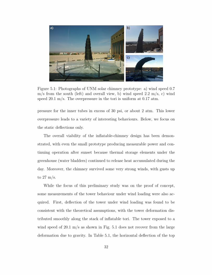
Figure 5.1: Photographs of UNM solar chimney prototype: a) wind speed 0.7m/s from the south (left) and overall view, b) wind speed 2.2 m/s, c) windspeed 20.1 m/s. The overpressure in the tori is uniform at 0.17 atm.
pressure for the inner tubes in excess of 30 psi, or about 2 atm. This lower
overpressure leads to a variety of interesting behaviours. Below, we focus on
the static deflections only.
The overall viability of the inflatable-chimney design has been demon-
strated, with even the small prototype producing measurable power and con-
tinuing operation after sunset because thermal storage elements under the
greenhouse (water bladders) continued to release heat accumulated during the
day. Moreover, the chimney survived some very strong winds, with gusts up
to 27 m/s.
While the focus of this preliminary study was on the proof of concept,
some measurements of the tower behaviour under wind loading were also ac-
quired. First, deflection of the tower under wind loading was found to be
consistent with the theoretical assumptions, with the tower deformation dis-
tributed smoothly along the stack of inflatable tori. The tower exposed to a
wind speed of 20.1 m/s as shown in Fig. 5.1 does not recover from the large
deformation due to gravity. In Table 5.1, the horizontal deflection of the top
32

of the tower with several measured wind speeds is presented.
Wind speed, m/s 0.8 ± 0.1 2.2 ± 0.2 3.1 ± 0.2 20.3 ± 0.3Deflection, m 0.12 ± 0.02 0.35 ± 0.08 0.51 ± 0.10 2.02 ± 0.06
Table 5.1: Horizontal deflection of tower top vs. wind speed.
5 10 15 20 25 30 350
0.05
0.1
0.15
0.2
0.25
k
!
Figure 5.2: Left: steady deflection angles computed from (3.7). Notice almost
linear dependence of φk on the height. Right: comparison of the shape given
by a convergent steady state of (3.7) with experiments for 2.2 m/s wind speed.
A detailed comparison of the tower deflection with wind speed in the static
configuration was performed corresponding to the medium wind speed – case
b) in Fig. 5.1. To do so, a constant wind speed throughout the vertical direction
was assumed, and a friction term proportional to −φ�(t) in the right-hand side
of (3.7) was introduced, which made the system converge to a steady shape,
independent of the friction coefficient. The result is shown in Fig. 5.2. All
the sizes of the tori and overpressures were taken to be exactly equal to their
experimental values. To match modelling with the experimental images, the
33

horizontal and vertical scales on the right hand side of the figure were chosen
to fit the immobilized bottom torus. Thus, the only fitting parameter was the
regularization constant � in (4.5) which was chosen to be � = 0.06. The reason
for the deviation of the scale at the top part of the experimental comparison
is perspective effect due to the fact that the deflection of the real tower is
not fully two-dimensional, and a small deflection of the tower in the direction
normal to plane of the photograph exists.
34

Chapter 6
Conclusion
Solar towers have been considered in the past for many years, however, despite
some of the advantages over other energy resources, there are many drawbacks
for rigid towers such as the costs of the construction and repairs. To circum-
vent this issue, inflatable towers made out of stacked toroidal elements has
been considered with the goal of reducing costs to build and maintain a solar
tower. The theory for the dynamics of inflatable solar towers has been devel-
oped and numerical simulations have been performed for the two dimensional
case. Experimental data has been collected and has shown to have agreement
between theory and real life experiments.
Future work should include the consideration of fully three dimensional
dynamics and optimal control theory by using the pressure of each individual
toroidal element as a control parameter. Larger prototypes can be considered
for a larger and more realistic wind profile and the data collected could used
to critique the overall viability of the inflatable solar tower design. There are
factors that must be taken into consideration when designing the inflatable
solar towers such as the costs of the control system. For example, the power
35

consumption of the control system will put a constraint on the speed at which
air can be pumped in and out of the tori. The efficiency of the tower should
also be considered as the production of energy should be comparable to other
traditional energy sources such as windmills and solar panels.
36

Bibliography
[Benoit et al., 2011] Benoit, S., Holm, D. D., and Putkaradze, V. (2011). He-
lical states of nonlocally interacting molecules and their linear stability: a
geometric approach. J. Phys. A: Math. Theor., 44:055201.
[Chi et al., 2014] Chi, M., Gay-Balmaz, F., Putkaradze, V., and Vorobieff, P.
(2014). Dynamics and geometric control of flexible solar updraft towers.
Proceedings of the Royal Society A, under consideration, pages 1–30.
[Ellis et al., 2010] Ellis, D., Holm, D. D., Gay-Balmaz, F., Putkaradze, V.,
and Ratiu, T. (2010). Geometric mechanics of flexible strands of charged
molecules. Arch. Rat. Mech. Anal., 197:811–902.
[Haaf et al., 1983] Haaf, W., Friedrich, K., Mayr, G., and Schlaich, J. (1983).
Solar chimneys part I: Principle and construction of the pilot plant in Man-
zanares. International Journal of Solar Energy, 2(1):3–20.
[Holm, 2008] Holm, D. D. (2008). Geometric Mechanics Part 2: Rotating,
Translating and Rolling. Imperial College Press.
[Holm and Putkaradze, 2009] Holm, D. D. and Putkaradze, V. (2009). Non-
local orientation-dependent dynamics of charged strands and ribbons. C.
R. Acad. Sci. Paris, Ser. I: Mathematique, 347:1093–1098.
[Mills, 2004] Mills, D. (2004). Advances in solar thermal electricity technology.
Solar Energy, 76(1-3):19–31.
[Putkaradze et al., 2013] Putkaradze, V., Vorobieff, P., Mammoli, A., and
Fahti, N. (2013). Inflatable free-standing flexible solar towers. Solar Energy,
98:85–98.
37

[Simo et al., 1988] Simo, J. C., Marsden, J. E., and Krishnaprasad, P. S.
(1988). The Hamiltonian structure of nonlinear elasticity: The material
and convective representations of solids, rods, and plates. Arch. Rat. Mech.
Anal, 104:125–183.
38

Appendix A
Numerical codes (MATLAB)
freedynamicswind.m
function freedynamicswind
%Solves the differential equations for the 2D case.
%Solves boundary value problem phi(tmax)=0, p(tmax)=p0
global n p0
clear all
p0=10^5; %Atmospheric pressure in Pa
n =20; %Number of tori
k=1:2*n;
y0phi=[0.1*ones(n,1); 0*ones(n,1)];%Initial conditions for phi, dphi
tmax_free=300;
nt=200;
tspan=linspace(0,tmax_free,nt);
[t,y]=ode15s(@freedynamics,tspan,y0phi);
tfree=t;
yfree=y;
phi0=yfree(nt,1:n);
dphi0=yfree(nt,n+1:2*n);
save(’./free_wind.mat’,’t’,’y’);
disp(’finished computation of free dynamics’);
function [dU,d2U]=hderiv(x,q,r)
eps = 0.06;
39

h=q.*sqrt(eps^2+sin(x).^2);
dh=q.^2.*sin(2*x)./h;
d2h=q.^2.*(2*cos(2*x)./(2*h)-sin(2*x)./(2*h.^2).*dh);
dU=3./4*q.^3.*sqrt(2*r./h).*dh;
d2U=3/4*q.^3.*sqrt(2*r).*(-1/2*h.^(-3/2).*dh.^2+1./sqrt(h).*d2h);
function dy=freedynamics(t,y)
%Free dynamics of the tower
global p0 n
n=length(y)/2;
phi=y(1:n);
dphi=y(n+1:2*n);
p0=10^5; %Atmospheric pressure in Pa
r = ones(n,1); %Inner radius in m
q = 3*r; %Outer radius in m
Rspecific = 287; %Specific R for air
T = 300; %Temperature in K
rho_air = 1.2; %Density of air
p=p0*ones(n,1); %All pressures are equal
p_shift=[p0 p(1:n-1)’]’;
rho = p/(Rspecific*T);%Mass density
m=pi^2*rho.*r.^2.*q; %Mass of tori
I0= (5/8*r.^2 + 1/2*q.^2.*m);%Moment of Inertia
delta_phi=[diff(phi)’ 0]’; %Delta phi_k
delta_phi_shift=[phi(1) diff(phi)’]’; %Delta phi_k-1;
height=2*cumsum(cos(phi).*r); %The first one needs to be modified
height=height-r(1);
A=q.*(r+pi*r); %Area exposed to wind
Torque=height.*A*wind(t).^2; %Torque due to wind
[U0prime,U0dprime]=hderiv(delta_phi,q,r);
[U0prime_shift,U0dprime_shift]=hderiv(delta_phi_shift,q,r);
d2phi=(p.*U0prime-p_shift.*U0prime_shift+Torque)./(I0.*p);
40

dy=[dphi ; d2phi];
function U=wind(t)
U=0*sqrt(10)*sin(0.1*t/pi).^2; %Wind speed m/s
41

processdynamicswind.m
function processdynamicswind
%post-processing the dynamics of solar tower with wind
clf
clear all
load(’./free_wind.mat’,’t’,’y’); clf
n=length(y(1,:))/2;
phi=y(:,1:n);
%plot(t,y(:,1:n));
%waitforbuttonpress
r = ones(n,1); %Sizes of tori in m
q = 3*r;
r1=[0 r(1:n-1)’]’;
nt=length(t);
h=(r+r1);
x=zeros(nt,n+1);
z=zeros(nt,n+1);
for k=1:nt
x(k,2:n+1)=cumsum(h.*sin(phi(k,:)’))’;
z(k,2:n+1)=cumsum(h.*cos(phi(k,:)’))’;
end
writerObj = VideoWriter(’tower.avi’);
open(writerObj);
set(gca,’NextPlot’,’replaceChildren’);
for k = 1:nt
clf
% plot(x(k,:),z(k,:));
hold on
for m=1:n
Lambda=[cos(phi(k,m)) sin(phi(k,m)); -sin(phi(k,m))
cos(phi(k,m))];
upvec=[0 r(m)]’;
sidevec=[q(m) 0]’;
rightup=Lambda*(upvec+sidevec);
leftup=Lambda*(upvec-sidevec);
42

x0=x(k,m+1)+[rightup(1) leftup(1)]’;
z0=z(k,m+1)+[rightup(2) leftup(2)]’;
line(x0,z0,’LineWidth’,2,’Color’,’k’);
rightdown=Lambda*(-upvec+sidevec);
leftdown=Lambda*(-upvec-sidevec);
x0=x(k,m+1)+[rightdown(1) leftdown(1)]’;
z0=z(k,m+1)+[rightdown(2) leftdown(2)]’;
line(x0,z0,’LineWidth’,2,’Color’,’k’);
sidecenter=Lambda*sidevec;
phi0=linspace(0,2*pi,20);
circlex=r(m)*cos(phi0);
circley=r(m)*sin(phi0);
plot(x(k,m+1)+sidecenter(1)+circlex,z(k,m+1)+sidecenter(2)
+circley,’k-’,’LineWidth’,2);
plot(x(k,m+1)-sidecenter(1)+circlex,z(k,m+1)-sidecenter(2)
+circley,’k-’,’LineWidth’,2);
end
plot(x(k,:),z(k,:),’r-’,’LineWidth’,1);
set (gca,’FontSize’,18);
axis equal
axis([-10 10 0 45]);
hold off
frame = getframe(gcf);
writeVideo(writerObj,frame);
end
close(writerObj);
43


![Solar updraft power plant chimneys - [email protected]](https://img.pdfslide.us/doc/110x75/6233d337a593ca6bb024bc49/solar-updraft-power-plant-chimneys-emailprotected.jpg)