Embed Size (px)
Citation preview

Dynamics of Analog Neural Networks
A thesis presented
by
Charles Masamed Marcus
to
The Department of Physics
in pania! fulfillment of the requirements
for the degree of
Doctor of Philosophy
in the subject of
Physics
Harvard University
Cambridge, Massachusetts
May, 1990

© 1990 by Charles Masamed Marcus
All rights reserved.
- II -

ABSTRACT
This thesis explores a variety of topics conceming the dynamics, stability and
performance of analog neural networks. Techniques used to study these systems include
global and local stabiJity analysis, statisticaI methods originaIly developed for Ising
model spin glasses and neural networks, numerical simulation, and experiments on a
small (S-neuron) electronic neural network. Attention is focused mostly on networks
with symmetric connections. The analog neurons are taken to have a smooth and
monotonic transfer function, characterized by a gain (i.e. maximum slope) f3.
The electronic network includes time delay circuitry at each neuron. Additional
circuitry allows measurement of the basins of attraction for fixed points and osciIIatory
attractors. Stability criteria for analog networks with time-delayed neuron response are
deri ved based on local analysis. These results agree well with numerics and experiments
on the electronic network.
A global stability analysis is presented for analog networks with parallel updating of
neuron states. It is shown that symmetric networks satisfying the criterion: 1/f3 > -Å.min
for all neurons, where Å.min is the minimum eigenvalue of the connection matrix, can be
updated in parallel with guaranteed convergence to a fixed point. Based on this criterion,
and a new analysis of storage capacity, phase diagrams for the Hebb and pseudo-inverse
rule associative memories are derived. Analysis of parallel dynamics is then extended to
a multistep updating rule that averages over M previous time steps. Multistep updating
allows oscillation-free parallel dynamics for networks that have period-2 limit cycles
under standard parallel updating.
It is shown analyticaIly and numerically that lowering the neuron gain greatly reduces
the number of local minima in the energy landscapes of analog neural networks and spin
- iii -

glasses. Eliminating fixed-point attractors by using analog neurons has beneficial effects
similar to stochastic annealing and can be easily implemented in a deterministic dynarnical
system such as an eleco-onic circuil.
Finally, a numerical study of the diso-ibution of bas in sizes in the Sherringwn
Kirkpatrick spin glas s is presented. It is found that basin sizes are distributed roughly as
a power law and that using analog state variables selectively eliminates small basins.
- iv-

ACKNOWLEDGMENTS
It is with pleasure and sincere thanks that l acknowledge the help, support, and
encouragement r have received while working on this thesis.
First of all, Bob Westervelt has been a terrific advisor. His intuition and sen se of
good, clean science has had a strong and positive influence on me. His guid anc e was
always present but never overbearing, and his insistence on clarity helped me greatly to
refine the ideas in thi s thesis into an inrelligible form. Bob has also managed IO create a
working environment that is filled with exciting physics and nice people. As a re sult, his
lab has always been a fun place IO spend time.
Sleve Strogatz has been a greal friend, teacher, and (IO use his word) partner. His
contributions to this thesis and IO my education are too many IO count.
Much of Ihe work in this thesis was done in collaboralion wilh Fred Waugh.
Working with Fred has been a real pleasure: easy, fun and remarkably produclive.
lam also especiaIly grateful IO the folIowing people for Iheir many contributions Io
myeducation: Larry Abbott, John Anderson, Ken Babcock, Roger Brockett, Jim Clark,
Jeff Dunham, Francis Everitt, Tom Kepier, Chris Lobb, Isaac Silvera, Paul Soko!, and
Alan Yuille.
lam grateful to AT&T Bell Laboratories for generously providing four years of
financial support.
Finally, l would like to thank my parenis, my sister, and my friends for Iheir support
and love.
- v -

Table of Contents
Abstract .... . .
Acknowledgments
Table of Contents
1. INTRODUCTlON
2. OVERVIEW OF THESIS
3. THE ELECTRONIC ANALOG NEURAL NETWORK 3.1.
3.2.
3.3.
3.4.
3.5.
Introduclion: Why build electronic hardware?
Circuitry
3.2.1.
3.2.2.
3.2.3.
Neurons ..
Analog dclay
Network. measurement and timing circuitry
Basins of attraction in 2-0 shces
Mea,uremenlS without delay .
Measuremenrs with delay . .
4. ANALOG NEURAL NETWORKS WITH TIME DELA y 4 .1. Introduction................
4.2. Dynamical equations for analog networks with delay
4.3. Linear stability analysis . . . . . . . .
4.3.1. Linear stability analysis with t = O
4.3.2. Frustration and equivalent networks
4.3.3. Linear stability analysis with delay
4.3.4. Symmetri C networks with delay .
4.3.5. Self eonnection in delay networks
4.4. Critical de1ay in the large-gain limit . ..
4.4.1. Effective gain a10ng the cohcrent osciIlatory attractor
4.4.2. Crossover from low-gain to high-gain regime
4.5. Stabihty of panicular network configurations
4.5.1. Rings . . . . . . . . . .
4.5.2. 2-0 lateral-inhibition networks
4.5.3. Random networks . . . . .
- vi -
iii
v
vi
1
7
11 Il
12
14
18
20
29 32
37
46 46
49
50
SI
54
55
59
63
64
66
71
73
73
76
83
4.5.4. Random symmetric dilution of the all-inhibitory network
4.5.5. Associative memories . . . . .
4.6. Chaos in time-delay neural networks
4.6.1. Chaos in neural network models
4.6.2. Chaos in a small network wilh a single time delay
4.6.3. Chaos in delay systems with non-invertible feedback
4 .7. Sum mary of useful results
5. THE ANALOG ITERATED·MAP NETWORK . 5.1. Introduction.......
5.2. lterated-map nctwork dynamics
5.3. A global stability criterion
5.4. Associative memory ...
5.4.1. Hebb rule
5.4.2. Pseudo-inverse rule .
5.5. Numerical results . . . . .
5.5.1. Verifying the phase diagnuns
5.5.2. Improved reeall at low gain: deterministic annealing.
5.6. Discussion......... .... ..
Appendix 5A: Storage capacity for the Hebb rule . .
Appendix 5B: Recall states of Ihe pseudo-inverse rule
6. TRE ANALOG MULTISTEP NETWORK 6.1. Introduction..............
6.2. Liapunov functi ons for multistep networks . .
6.2.1. Global stability criterion for general M
6.2.2. The case M = 2: Only fixcd points and 3-cycles
6.3. Application to associative memorics
6.4. Convergence time . . . . . .
6. 5. Conclusions and open problems
7. COUNTING ATTRACTORS IN ANALOG SPIN GLASSES AND NEURAL NETWORKS .. 7. I . Introduetion: deterministic anncaling
7.2. Counting attractors: analysis
7.2.1. Analog spin glass .
7.2.2. Analog neural network
7.3. Counting attractors: numerical results
7.3. 1. Technique for counting flXcd points
- vii •
85
90 91
91
96 97
101
103 103
104
109
112
114
117
121
121
125
125
127
132
136 136
140
140
146
148
151
158
162 162
167
167
178
187
187

7.3.2. Numerical results for analog spin glass
7.3.3. Numerical results for neura! network .
7 A. Discussion.. .. ...........
7.4.1.
7.4.2.
Appendix 7 A:.
Appendix 7B:
Appendix 7C:
Asymmelry: An altemate way to eliminate spurious attmetors.
A shon discussion of allmelDrs in mullistep systems
(det (A)}T for analog spin glass
Expansions for steepest descent integrnls
(det (A))~ for neural network ....
8. THE DISTRIBUTION OF BASIN SIZES IN THE SK SPIN GLASS .. ... . 8.1. Introduelion: back to basins . .
B.2. Probabilistic ba~in measurement
8.3. The disoibution of basin sizes .
8.3.1. Definitions.. . . .
8.3.2. Numerically observed power·!aw behavior ofj{W)
8.3.3. Conscquenees of a power law distribution of basin sizes
8.4. Disoibutions for other models . . . . . . . . .
804.1.
804.2.
8.4.3.
Clusters of states in the SK model. . .
The Kauffman model and the random map
The 1·0 spin glass ...
B.5. Basin sizes in an analog spin glass
8.6 Discussion and open problems
9. CONCLUSIONS . .... .
IO. APPENDIX: DYNAMICS OF CHARGE DENSITY WAVE SYSTEMS WITH PHASE SLIP . . . . . . . . . . . . ..
10.1. Reprin!: S. H. Strogatz, C.M. Marcus, R. M. Wcstcrvelt, and
R.E. Mirollo, "Simple Modelof Collective Transpon
with Phase·Slippage", Phys. Rev. Let!. 61, 2380, (1988)
10.2. Reprin!: C.M. Marcus, S.H. Strogatz, R.M. Westervel t,
"Oelayed switching in a phase·slip modelof charge·
density·wavc transport", Phys. Rev. B 40, 5588, (19B9)
References . . . . . . . . . . . . . . . . . . . . . . . . .
- vw -
190
190
195
195
197
202
205
208
213 213
215
219 219
222 224
227
228
230 232
234
236
238
. . 242
243
247
252

Chapter 1
INTRODUCTlON
Our world is filled with complex phenomena which emerge, as if by magic, out of
interactions among many simple elements. Sometimes (rarely) an intellectually satisfying
picture can be painted, allowing us to claim that we understand how the magic comes
about. For certain static phenomena, statistical mechanics provides such a picture, and
makes clear how the interaction of microscopic elements can give a large system a "life of
its own," with well-defined properties that are not obviously present when the system is
observed element by element. Statisticai mechanics also provides a justification for the
empirical faet that large systems can be characterized by a few well-chosen quantities; one
does not need to keep track of all 1023 variables. This feature is essential for rendering
large systems understandable.
Extending the principles and techniques of statisticaI mechanics to include complex,
dynamic phenomena on a macroscopic scale remains an outstanding challenge and a
problem of great current interest in many areas of physics. Ultimately, one would like to
understand the complexity of the real world within a framework linking statisticaI
mechanics and dynamical systems theory. The hope for such a synthesis, however,
rests on the hypothesis that microscopic proces ses ean be described by simple models. lf
the complexity of nature must be accounted for at all size scales, we certainly have no
hope of understanding big systems.
Neural networks research certainly represents the most extreme test of the hypothesis
that complexity can emerge directly out of the interaction of a large number of simple
elements. It asks the question, "Can the operation of the most complicated object known
- l -

be described as an emergent propeny of maximally simple elements interacting according
to simple rules?" This line of inquiry does not presuppose that the answer is yes, but
rather seeks to discover just how far such a princip le can go. Judging from our current
levelof knowledge about even the simplest biological systems, we may not leam whether
the approach is justified for some time, let alone reap (and market) the fruits of the
endeavor.
In addition to the role of neural networks as a paradigm for understanding biology,
there is a purely technological motivation for developing highly parallel dynamical
systems that can solve difficult problems. Simply put, the standard computer architecture
is coming to the end of its rope. Many problems of great technological interest cannot be
sol ved with acceptable speed using the fastest conventional computers, and even allowing
factors of 100 or 1000 in speed, the present technology remains ill-suited to cenain
applieations. It is interesting to note that many tasks whieh are routinely performed by
humans with almost trivial ease seem to be the most ehallenging for computers. Our
ability to quickly recognize a face, or to infer the shapes and distances of objects from
visual information illustrates the aSlronomieal superiority of biological computation over
current computer technology. What makes this superiority more remarkable still is the
faet that the fundamental time scale in biology is around a millisecond, some four orders
of magnitude slower than standard computer cycle times.
The efficieney of biological computation suggests that perhaps by simply emulating
biology's basie design - without necessarily duplieating it - we may realize revolutionary
technological advances. Which qualities constitute biology's "basic design" is currently
anybody's guess, though massive parallelism and fault tolerance seem to be two such
basic principles, at least in the conex. (Neither feature is part of the basic design of
current computers.) If not hin g else, biological neural networks serve as working
demonstrations that a vastly superior technology is pos si ble in principle .
- 2 -

We will not review the long and interesting history of neural networks here. Instead,
we refer the reader to several good reviews which have appeared recently [Lippmann,
1987; Grossberg, 1988; Amit, 1989; Hirsch, 1989; Abbott, 1990; reprints ofmany ofthe
cJassic articJes can be found in Shaw and Palm, 1988]. The various accounts of neural
networks are remarkably disparate, especiaIly in their historicai perspective, so it is
necessary to read several versions in order to appreciate the breadth of the subject.
A common feature of nearly all neural network models, dating back to their modem
origin in the work of McCulloch and Pius [19431, is the sum-and-threshold device
known as a formal neuron or simply a neuron for short 1. The basic neuron we consider
is shown in Fig. 1.1 (many variations will appear later). The output of the formal neuron
ean be binary ( (O,I) ar (-l,!) ) or continuous, but the sigmoidal (s-shaped)
nonlinearity of the input-output transfer function is standard. Much more will be said
later regarding the shape of the neuron transfer function. A neura! network is typically a
collection of these formal neurons arranged in some architecture, with neuron inputs
connected to extemal signals and to the outputs of other neurons. Connections between
neuron s are characterized by a set of connection weights, which may be negative,
positive, or zero. In addition, one must specify a dyn arni c rule defining how the states of
the neuron s change in time.
The hard part of the problem, of course, is figuring out how to connect the neurons to
each other so that the resulting dynamical system will do something imeresting ar useful.
The idea, however, is not to set the connections "by hand," but rather to develop leaming
algorithms so that the network can respond to extemal stimuli by modifying its own
connections in an effective way. Loosely speaking, we would like the network lo leam
from its own experience. Considerable progress in this area has been made, particularly
for the lask of associative memory, beginning with the work of Hebb [1949), and
l Henceforlh, lhe word "neuron" will be taken to mean a formal neuron; any references to real (biological) neurons will be explicitJy stated as such.
- 3 -
continuing through to the recent work of the PDP Oroup fRumelhart et al., 1986], E.
Oardner [1988], and others. Hebb's primary contribution was to postulate aremarkably
simple, yet effective mechanism for modifying conneclions which will store a particular
neural slate as a memorized pattern. The rule is Ihe folIowing: Tmpose a pallem of
stimulus onto the network, and incrementally inerease the connection weight between
neurons with eoincident aClivity. This modification will eventually cause the imposed
pallem of neuron al aClivily to become a stable configuration of the system af ter the
stimulus is removed. There is evidence that Hebb's mechanism is realized in biological
systems, though at present this is an is sue of considerable debate [Lynch, 1986].
An important milestone in the understanding of neural network models was the recent
work of Hopfield [1982; 1984; Hopfield and Tank, 1985; 1986]. Hopfield (and later,
Hopfield and Tank) emphasized four ideas, all of which have proven extremely fertile.
Those ideas were: (I) there is a close analogy between neural network models with
extensive feedback and random magnetic systems known as spin glasses; (2) the
dynamical aspects of networks can be anaTyzed in terms of an energy function; (3) simple
neuraT networks ean be mapped onto traditionally difficult computational problems,
yielding good, fast resulls; and (4) neural network models can be naturally realized in
analog electronics. It could be argued thai, in fael, none of these ideas was new. The
conneclion between neural networks and magnelism, for example, dales back to the
19505 [Cragg and Temperley, 1954], and the energy function idea had also been used by
Cohen and Orossberg [1983; Carpenter et al., 1987]. The com bi nation of ideas,
however, along with tangibie results and a clear exposition in a style familiar to
physicists, managed to generate an excitement within the physics community which has
proven to be both contagious and self-sustaining.
Many of the topics addressed in this thesis spring directly from the four ideas of
Hopfield mentioned above. Most of Ihe Ihesis will focus on various dynamical
- 4 -

properties of analog neural networks of the type described by Hopfield (see Fig. l.l),
with an emphasis on the practical, rather than the biological. The goal throughout will be
to discover useful - and whenever possible, simple - results which ean serve as
guidelines for Ihe design offasl, parallel compuling devices. Oceasionally, the relevance
of a resull to biology will be menlioned, but we stress al the outset that sue h insights are
of seeondary importance in thi s work.
The main eonclusion of the thesis is that the input/output transfer funclion of Ihe
individual neurons greatly influences the eolleetive dynamies of the whole network.
Furthermore, for the restricled class of models eonsidered, Ihe nature of this influence
can be analyzed and described quantitatively. From a practieal point of view, this thesis
demonstrates that analog neural nerworks have important computational advantages over
eorresponding models eonstructed from binary neurons. Thus, in emulating biology to
make fast parallel computing machines, one is likely to find that the analog character of
the neuron is an important aspect of Ihe computalional power of the syslem as a whole.
Chapler 2 gives a more detailed overview of the topies presented in this thesis,
chapter by chapter.
- 5 -

FORMAL NEURON
\ SUMMING POINT
Fi(h;)
HOPFIELD-TYPE (FEEDBACK) NEURAL NETWORK
CONNE WEIGH
T;}
CTION T
~
INPUT LI NE
\
~ I
-f'>--
.,.;:
BINARY NEURON TRANSFER FUNCTION
Sgn(f4) f---
---+---h;
ANALOG NEURON TRANSFER FUNCTION
Fi(h; )
---!---h;
Fig. I . I. The basic elements of the neural network model discussed in this thesis. Many variations will appear later. The formal neuron (or just "neuron") has an input h; which is a weighted sum of the outputs from other neurons. The connection weight from neuron j to neuron j is given by the matrix element Ti}' The neuron output is a non linear function F/h;) of the input. This function is typically either binary or a continuous sigmoid (s-shaped) function. The network architecture we consider has extensive feedback, and we will frequently impose the symmetry condition (T;) = T}).
- 6 -
Chapter 2
OVERVIEW OF THESIS1
This thesis addresses a variety of IOpics, mostly involving the dynarnics, stability,
and performance of analog neural networks. There are, however, many sections and
even whole chapters (Ch. 8 and Ch. IO, for example) which depart from this subjecl. A
consistent theme throughout the work concerns the dynamical behavior of nonlinear
systems with many degrees of freedom. A variety of techniques will be used to explore
these systems, inc1uding experiments, numerical investigations, and mathematical
analysis.
In chapter 3, we describe an electronic analog neural network consisting of eight
neurons bui It using operation al amplifiers with nonlinear feedback , and accompanying
circuitry to allow fast measurements of the basins af attraction for fixed points and
oscillatory modes. Af ter providing construetion details , we present several
measurements of the shapes of the basins af attraction in an analog associative memory.
A notable feature af the network is the inc1usion of charge-coupled device delay lines in
each neuron. Delays are adjustable over nearly two orders of magni tude, allowing
delay-induced instabilities to be studied experimentally, and eriticaI values of delay to be
measured in a variety of network configurations, and as other network parameters are
varied.
In chapter 4, we con sider the effect of time delay an the stability of symmetrically-
connected analog neural networks from a more mathematicaI point of view. We present
l References have been strippcd from this chapter to keep it short and easy to read. See subsequent chapters for references.
- 7 -

two stability criteria, based on local stability analysis, that give <.-TItica! values of delay
above which sustained collective oscillation appears. The surprising resuh is that the
critical delay depends on only a few network parameters: the characteristic time of the
network, the neuron gain, and the exrremal eigenvalues of the connection matrix. Resuhs
are applied to several network configurations, including symmetrically connected rings,
two-dimensional lattices of neurons, randomly connected networks, and associative
memory networks. Results are found to be in good agreement with numerics and
experiments performed on the elecrronic network. Finally we discuss chaotic dynarnics
in time-delay networks, and give an example of a three-neuron circuit with delay-induced
chaos.
In chapter 5 we study the stability and associative-memory capabilities of a discrete
time, analog neural network with parallel updating of neuron states. Parallel operation is
crucial to the design of fast neural networks. The usual practice for discrete-time systems
with binary neurons, however, is to update sequentially in order to prevent unwanted
oscillation. We show that all oscillatory modes can be eliminated from a parallel-update
analog neural network with symmetric connections by lowering the neuron gain belowa
certain critical value. The result is stated as a simple, global stabil it y criterion relating the
maximum neuron gain and the minimum eigenvalue of the connection matrix. This
criterion allows "safe" parallel dynarnics, with guaranteed convergence to a fixed point.
Following this, we apply the analog nerwork to the problem of associative memory, and
present novel phase diagrams (in terms of neuron gain and the ratio of stored patterns to
. neuron s) for the Hebb and pseudo-inverse learning mies. To our knowledge, these are
the flTst reported analytical results of storage capacity for analog neural nerworks. Within
the "recall" regions of the phase diagrams, where memory pattems are stable and have
large basins, we find numerically that the performance of the associative memory
improves as the neuron gain is lowered. This important observation, also noted by
Hopfield and Tank and others, suggests the possibility of deterministic analog annealing.
- 8 -

In chapter 6 we generalize the stability analysis af chapter 5 to include analog
networks with an update mIe based an an average over M previous time steps, for
arbitrary M. Standard parallel updating eorresponds to M = 1. The important result is
that the eritical value of neuron gain is increased for the multiple-time-step update rule by
a factor of M, compared to standard parallel updating. Some applieations to associative
memories are then given. We also present a simple analysis of the eonvergenee rate of
the multiple-time-step network as a funetion of M.
In chapter 7 we study the number of loeal minima in the dynamieal (energy)
landseape of the analog spin glas s and the analog associative memory. We show that the
expected number of local minima (NIp) for both systems increases exponentially with the
size of the system N, as (N fp) ~ exp(aN). The sealing exponent a depends on the
neuron gain for the case of the analog spin glass, and depends on both the neuron gain
and the ratio ofpattems to neuron s for the analog associative memory. Analytieal values
for a are given for both systems. As neuron gain deereases, the value of a (for both
systems) also deereases, which has the effect of dramatically reducing the number of
loeal minima. These results provide an analytieal framework for understanding how
lowering the neuron gain ean lead to improved performance in analog associative
memories. Numerical observations of this effect are also presented in Ch. 5. Theoretieal
values for the scaling exponent a agree reasonably well with numerical values found by
directly counting the fixed points in a large sample of eomputer-generated realizations.
In chapter 8 we explore the basin structure of the detenninistie (zero-temperature)
SK spin glass. This model has been studied extensively and is known to possess an
extremely rieh energy landscape. The main result of this chapter is that the numerieally
measured distribution of basin sizes, averaged over realizations, obeys a power law with
exponent near -3/2 over a wide range of basin sizes. The exponent of the power law
appears to be independent of N . Some consequences of this power law are then
- 9-

considered. The distribution of basin sizes in the detenninistic SK model is qualitatively
different from other c10sely related distributions which, among themselves, show certain
universal features. Apparently, and perhaps surprisingly, the universality seen in these
other distributions is not shared by the distribution observed here. We end this chapter
by showing (again, numerically) that the distribution of basin sizes is strongly affected by
the use of analog state variables. We find that redueing the gain in an analog spin glass
selectively eliminates fixed points with smal l basins of attraetion.
In chapter 9, we give some brief conclusions and remarks eoneerning unsolved
problems and interesting fUTUre directions.
Chapter IO is an appendix containing two papers on the dynamics of charge-density
waves (CDWs). This work is essentiaIly unrelated to neural networks, though it shares
with the previous chaplers a general Iheme of collective dynamics in nonlinear, many
body systems. The main idea in these papers is that a simple modification to allow phase
slip in a previously-studied mean-field modelof CDW dynamics eau ses the smooth
depinning transition to become discontinuous and hysteretic. The behavior of the phase
slip model is very suggestive of switching, which is observed experimentally in eertain
CDW systems. The way that phase slip is introduced in Ihis model has the added virrue
of making the system analytically tractable.
- 10 -
Chapter 3
THE ELECTRONIC ANALOG NEURAL NETWORK
3.1. INTRODUCTION: WHY BUlLD ELECTRONIC HARDWARE?
Soldering gives a person lots of time IO think. One partieularly deep question to think
about while soldering together an e1eetronic neural network is what distinguishes an
experiment from a simulation, or, in other words, why build (his circui(? Among neural
networks researchers, (here is a large camp of non·apologists who view the mathematical
system as the neural network, rather th an considering the equations to be a simplified
description of some physical reality [see the discussion of Maddox, 1987]. From thi s
perspective, an e1ectronic neural network serves as a fast analog computer for simulating
the "real" (mathematica!) system. A more engineering-minded line of thought emphasizes
the potential for building powerful computational devices. Because microelectronics, and
particularly VLSI, is the likely medium for implementing these devices [Mead, 1989], it
is important (the argument goes) to learn as much as pos si ble about real circuits and the
behavior of large, interconneeted e1ectronic networks. By this reasoning, building an
e1ectronic network from discrete componenls is progress loward the ultimale goal of
building a "real" neural network (i.e. a large, fast and truly useful piece of e!ectronic
hardware).
Apart from these bigger questions of motivation is the simple faet that many imponant
problems in neural networks (especially analog neural nelworks) are difficult to treat
analYlically or by conventional numerical simulation. Occasionally, such problems ean
- 11 .

be studied easily and directly in a small electronic network. Af ter presenting the details of
our circuit in §3.2, we will con sider two problems of this son. Theyare:
(l) What are the shapes - not just the volumes - of the basins of attraction for tlle
recalt states of an associative memory? In a well-designed associative memory, the
basins of attraction for recall states should be large, but that is not sufficient: the basins
must also be roughly spherical (by some appropriate measure) and centered about the
recalJ states. If the basins of attraction are diffuse or disconnected in stale space, the
memory will not be usefuL In § 3.4 we show that the shapes of the basins for recall
states are in faet somewhat irregular when the network is overloaded with memories.
(2) How does time delay affect the transients, attractors and basins of attracrion in a
neural nelWork? This problem is of paniclllar interest to the engineering-minded camp,
as the operating speed of VLSI circuitry willlikely be limited by switching-delay-indllced
instabilities (for a discussion of delays in VLSI, see [Mukherjee, 1985, Ch. 6]). MllCh
of the mathematical analysis of networks with time delay that appears in chapter 4 was
suggested by or confumed using the electronic network.
Electronic circllits have also been used to find and characterize chaOlic behavior in
analog neural networks [Marcus and Westervelt, 1989b; Kepier et al., 19891. This
application will be discllssed in § 4.6.
3.2_ CIRCUITRY
In this section we provide a detailed description of the electronic nellral network
circuit. First, thOllgh, we give a quick overview of the circllit's main features:
The electronic network consists of eight analog neuron S (nonlinear amplifiers)
connected via 128 manual switches and resistors. Connections between pairs of neuron s
ean be noninverting, inverting, or open, depending on the positions of these 128
- 12-

switches. Each neuron has an independently adjustable gain and saturation level, and has
a time delay section based on a charge coupled device (CCD) analog delay line. (The
reader may wish to glance ahead at Fig. 3.4 at this point.)
The dynamicaI equations for the voltages ui(r) on the input capacitors of the neurons
(nonlinear amplifiers) are
N
+ L 7;; tAuj(r' - Tj)) i = 1 '0'0' N, (3.1) j = l
where ei is the neuron input capacitance and Ri = (:EjITi})-! is the resistance to the
rest of the circuit at the input of neuron j , and f; is a smooth sigmoid function describing
the transfer function of the jlh neuron. Equation (3.1) is identical to the analog system
described by Hopfield [1984], with the inclusion of time delay. It is not equivalent,
however, to some other hardware implementations which have the input capacitor across,
rather than in front of, the nonlinear amplifier [Denker, 1986c; Amit, 1989; KepIer er al.,
1989].
Digital timing circuioy and voltage-controIled analog switches are used to periodicaIly
op en the feedback path from the resistor matrix to the neuron input and load initial
conditions onto the neuron s' input capacitors. The initial conditions are determined by
eight independent voltages, any two of which can be raster-scanned using independent
function generators. At the same time, the two function generators are used to position
. the beam of a storage oscilloscope (Conographic 611). When the state of the network
matches some reference state (which has been set with manual switches), the beam of the
storage oscilloscope is tumed on, and the resulting pattern on the storage oscilloscope
shows an image of the basin of attraction for the reference state in a two-dimensional slice
of initial condition space. Alternately, the oscilloscope beam ean be set to go on only
when the circuit enters an oscillatory state, thus iIImninating a slice of a basin of attraction
- 13 -

for oscillation. Neuron outputs can also be displayed directly (as X vs. Y, for any pair of
neurons) using a second storage oscilloscope (Tektronix 611). The time scale for a
complete load/run cyc\e is adjustable, and is typically -10-40 ms.
The folIowing three subsections provide the detaiIs of the various pans of the circuit.
3.2.1. Neurons
The schematic for an individual analog neuron is shown in Fig. 3.1. Each neuron
uses four JFET operational amplifiers (op-amps), all on a single 14-pin integrated circuit
(National Semiconductor LF374N). Staning at the input side of the neuron, the first op
amp serves as a unit y gain buffer, giving the neuron a high input irnpedance. The second
op-amp, with diodes in the feedback , is the nonlinear pan of the circuit, giving the
neuron its sigmoidal or saturating transfer function, as discussed below. The third op
amp serves as a variable gain amplifier and sets the overall amplitude of the output. Next
in the signal path is the CCD delay (see: § 3.2.2 below), which can be switched in or out
independently for each neuron. Finally, the fourth op-amp inverts the output lO allow
inhibitory as well as excitatory connections.
The neuron transfer function J (dropping the subscript i) is defined by the relation
J(input) = output, where output refers to the neuron's noninverting output. The
function J is made interesting by the diodes in the feedback path of the second op-amp.
To derive an expression for J, we stan with a simple form for the cUlTent-voltage (I-V)
characteristic of a diode [see: Sze, 1981, § 2.4)
(3.2)
The parameters Is = 2.9 X 10⁻⁵ mA and VT = 5.9 X 10⁻² V were determined by a least-
- 14 -

---"1+ INPUT
'14 LF347
Al (.oK TRIM)
+ 1/4 LF347
INPUT
Fie:. 3.1. Schematic diagram of analog neuron.
- 15 -
,--_________ INVERTING
OUTPUT
"'>*"-___ INVERT1NG
.... OUTPUT +
114lF347
> __ INVERT ..... G
OUTPUT
'---- tNVERTING OUTPUT

square fit to data in the manufacturer's data sheet for the diode used, which was the
1N914. Equation (3.2) and standard op-amp circuit ana1ysis (Le., the principle ofvirtual
nu II) give the folIowing implicit expression for f,
(3.3a)
v = ([2~~]) output, (3.3b)
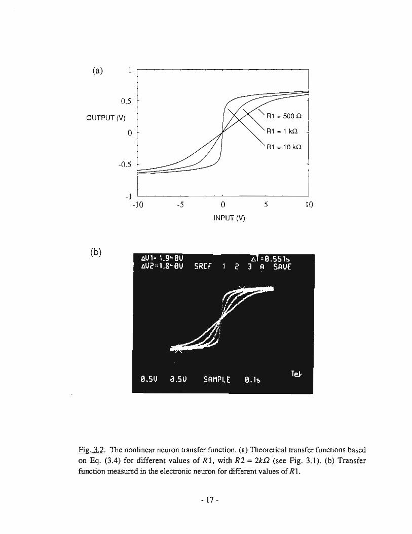
where the resistance values from Fig. 3.1 are shown in square brackets. Figure 3.2
shows the neuron output as a function of its input as given by Eq. (3.3) for different
values of RI, with R2 held fixed at 2 kil and numerical values for Is and Vr
inserted. For large and small signals, Eq. (3.3) can be expanded to leading order to give
( RlR2]. oUlput = 2 tnpll!
10 (W) (for smal! signals, linear regime), (3.4a)
OUlpll! = [ R2]11l([ inp~t ) (for large signals, Safuratedregime). 2kil Skil Is
(3.4b)
The crossover from the linear to the saturated regime occurs when
input - ([S~~])Vr. (3.5)
The maximum slope of the neuron transfer function, defined as the neuron gain {3, will
be very imponant for all som of analysis in later chapters. From (3.4a), we can
- 16 -
Ca) l
0.5
OUTPUT (V) "R1 = 500 O
J O R1 = 1 kO
R1 = 10 kO
-0.5
-l I -10 -5 O 5 10
INPUT (V)
(b)
Fig. 3.2. The nonlinear neuron transfer function. (a) Theoretical transfer functions based
on Eq. (3.4) for different values of RI, with R2 = 2kfl (see Fig. 3.1). (b) Transfer function measured in the electronic neuron for different vaJues of RI.
- 17 -

irnmediately identify the neuron gain,
( RI R2 J
f3 = 1O(W)2 . (3.6)
Notice from Eq. (3Ab) that for latge signals, the neuron output saturates to a logarithmic
function of the input. This behavior is different than the tanh function - the canonical
sigmoid - which saturates to a hatd limit at large atgument. In practice this difference
does not appeat to be significant.
3.2.2. Analog delay
The schematic for the analog delay circuit is shown in Fig. 3.3. Each neuron has its
own independent delay circuit, which can be switched in or out manually. The heart of
the circuit is a charge-coupled device (CCD) analog delay line, RD51 06A, manufactured
by EG&G-Reticon. The RD5106A chip is a so-called "bucket-brigade" device. The
device operates by charging an input capacitor to the instantaneous (analog) input voltage,
and then passing that chatge along a brigade of 256 subsequent capacitors, with each
transfer of charge !riggered by a pair of pulses from an extemal clock. At the end of the
brigade of capacitors, the chatge is converted back to an analog voltage which constitutes
the output signal. The time -( taken to traverse the entire brigade (i.e. the delay time) is
related to the clock frequency f c/ock by:
, [ l __ 0_.5_12_ T ms =
fclock[ MHz l (3.7)
The shortest delay available from this chip is nominally 300ps (fe/ock = 1.7 MHz),
• 18 -

FUNCTION ...n.J"L GENERATOR
L 17 12.3V 1SV
,>"'
-
1 K 49.9K 100K 3K
1 O 90K 10K
.1SV 6 RD510I)A 4 . 1SV
100K + 100K 100K:
1/2 LF4 12 100K
100K 100K
IN OUT
I t"~~~Vt I IN OUT
Fie:. 3.3. Schematic for analog delay circuit. The entire circuit (excluding the voltage regulator section) is duplicated for each neuron. The heart of the circuit is the EG&G Reticon RD5106A charge coupled device analog delay line.
- 19 -

although the appearanee of de offsets limits the usable range to r' > -450 Jls
lfc/ock < 1.2 MHz). On the long-delay end, the chip itself is good up to delays
exeeeding one second, but in practice the delay is limited by a "bucket discretization
noise" at a frequency fnoise[kHz] = 256/(r'[ms]). The nelwork itself will filter out
this noise as lang asfnoi.<e is well above rhe network's bandwidth, which is in the range
l - 8kHz depending an the connection matrix (see next subsection). This gives a range
of delay covering nearly two orders of magnitude:
450ps < r' < - 30ms . (3.8)
Because all delay eircuits are clocked using the same function generator, all delays (when
switched in) are identical. It would be very simple to construet individual on-board
trigger circuits using LMS5S's to allow independent delays.
The rest af the delay circuitry is mostly used to get around ane unfortunate aspect af
the CCD delay line, which is that input voltages must be positive. The first op-amp is
used to add an adjustable de offset to the input signal, and the seeond op-amp is used to
remove that offset. The second op-amp also has adjustable gain to eompensate for the
RD5106A not being exactly unit y gain . All offsets and gains are independently
adjustable via three trim-pots per delay circuit. There is also a 10 kHz low pass filter
section between the delay line and the second op-amp, to remove bucket discretization
noise. Finally, a single voltage regulator (National Semiconductor LM317L) is used to
supply the required 12.3 V to all eight RDS i06A's.
- 20-

3.2.3. Network, measurement and timing circuitry
A. The nerwork
Figure 3.4 shows the layout of the entire network. A single circuit element in a box
represent multiple idemical components: 8 delay-neurons, 8 initial condition loaders, 8
output buffers (LM74 l 's), and 64 resistor-switch interconnect crrcuits. The characteristic
relaxation time of the network (without delay) is determined by the interconnect
resistances and neuron input capacitance. For interconnect resistances (T'ij)-l =
IOOk.!2 and input capacitances C i = lOnF, the network relaxation time is l/n [ms],
where n is the number of neurons connected to the input of any given neuron. The
characteristic relaxation time for the eIectronic network can easily be varied over a few
orders of magni tude by replacing the input capacitors, which are installed using plug-in
connectors. Indeed, the entire circuit could be sped up considerably, with characteristic
times in the tens of microseconds, without pushing the bandwidth of any of the integrated
circuits; the limiting factor is the delay, which cannot be less than 450 Jls. The
characteristic time to load initial conditions is (lO kQ)(lO nF) = 100 JlS.
- 21 -

y
STORAGE SCQPE.-1 (BAS IN PLanER)
FUNCTION
zf--_---1 ATIAACTOA IDENTlFIEA
FROM TIMING f---4f---' CIRCUIT IEI
STORAGE SCOPE.-2 (TRANSIENT PLOTTER)
z
100K
__ -+====~~_--,FROM TIMING r CIRCUIT (B)
1/2 A07512
FROM TIMING CIRCUIT (C)
Fig. 3.4. Schematic diagram of the entire network. Single devices in boxes represent multiple devices: 8 each of the neurons. run/load sections. and LM741 buffer; 64 of the resistor-switch pairs. Storage oscilloscope #1 is used to plot slices of basins of attraction; storage oscilloscope #2 is used to plot the outputs of any pair of neurons as X vs. Y. The source of the various timing signals is shown in Fig. 3.6.
- 22-

B. Attractor ldentifier
The box marked "attractor identifier" in Fig. 3.4 is shown in detail in Fig. 3.5. This
circuit is used to test if the network has settled onto a specified fixed point attractor or,
alternately, to determine if the network is in an oscillatory mode.
The part of the attractor identifier circuit marked "fixed-point attractor identifier" (the
larger dashed box in Fig. 3.5) works as follows: First, eight comparators (LM311 's) are
used to convert the analog state of the network into eight thresholded digital (TIL)
signals. This eight-bit digital state is then compared bit by bit to a reference state, which
has been selected by positioning eight manual switches. The reference state might be, for
example, a programrned memory pattem. If all eight bits of the network state match the
reference state, then the line leaving the fixed-point section is set high, otherwise, it is set
low.
The part of the attractor identifier marked "oscillation detector" (the smaller dashed
box in Fig. 3.5) uses a retriggerable l-shot (96LS02) with a high-time that is set to be
longer than the period of oscillation under investigation. If the comparator undergoes a
state transition within the high-time of the l-shot, the output of the l-shot remains in a
high state. If the output of the comparator remains fixed - because the neuron being
observed has stopped oscillating - the l-shot goes low at tlle end of its current high-time.
The high-time of the l-shot ean be continuously varied from 4.3 ms to 8.6 ms via an
extemal potentiometer. Note that an oscillating neuron must cross zero output in its
excursion to trigger the oscillation detector.
Where the fixed-point and oscillation detectors come together there is a bit more
digitallogic, and another manual switch. Depending on the position of this switch , the
TIL output which goes to a sample/hold (AD583KD) indicates one of the two folIowing
conditions:
- 23-

1- OSCILLATION DETECTOR _ - l
SWITCHES TO SPECIFY STATE OFINTEREST
FROM SELECTED NEURON
SV
3.3K
~ -/-~~~~ON:-11-5V LM311
! ~;>-~"' I
FROM NEURON~
I -
SV
3.3K
5V
,.:p!+:::::-:"~1 DOK I O.l!!F lOOK
961S02 (RETAlG. l-SHOT)
-I
TO STORAGE
SCOPE'l
Fig. 3.5. Schematic for anractor identifier circuit
- 24-
FIXED-POINT I OSCILLATION DETECTOA SWITCH
/ TO
r==" STORAGE AD583KD SCOPE II (SAMPLE & HOLD)
FROM TIMING CIReUrT (E)
ATTRACTOR IDENTIFIER
FROM TIMING CIRCUIT (E) SAMPLEIHOLD TRIGGER
11111111 FROM NEURONS (VIA BUFFERS)

Swirch up: [selecled neuron is osciJlating]
Switch down : ([network state matches reference state]
AND
r selected neuron is not oscillatingll.
The combined logic for the Swirch down position insures that all matches to the
reference state are acrual fixed points, not oscillatory modes or transients.
C. Timing
The timing signals appearing in Figs. 3.4 and 3.5 are supplied by the digital (TIL)
circuit shown in Fig. 3.6. Also shown in Fig. 3.6 are TIL logic stales
(low = av, high = 5 V) as a [unclion of time at several points in the timing circuit,
labeled (A) - (E). Trace (B) is the run/load signal sent to the voltage-controlled analog
switches; trace (E) is the "sample now" signal sent to the sample/hold in the attrdctor
identifier circuil. The time between when (B) goes low (ne twork feedback path
reconnected) and when (E) goes low (state of the system sampled by sample/hold)
defines the allowed settling time of the network. This value is adjusted to be -5-10 times
the nerwork relaxation time, so that nearly all transients have died out by the time a new
"sample now" signal is sent. When delays are used, the allowed settling time must be
quite long, as indicated in the table of Fig. 3.6.
Examples of network dynamics are shown in Figs. 3.7 and 3.8. Figure 3.8 shows
that in addition to creating sustained oscillatory modes, delay can induce extremely long
and complicated transients when the circuit converges to a fixed point. Long, delay-
induced transients were also investigated by Babcock and Westervelt [1986b].
- 25-

LM555 (A) (D) -- 112 74221 r---(CLOCK) ('·SHOT)
t (A)
74121
('·SHOT)
li)
(A)
112 7.4221 --{) (E)
TOATIMCTOR IDENTlF IER (SAMPLEJHOlD TRIGGER) ('·SHOT)
(B)
(C)
TO FET ANALOO SW ITCHES (RUN'LOAD SIGNAL)
TO STORAGE SCO PE '2 NKER) (RETURN BEAM BLA
(B)_---'nL __ -lnL... __ --'nL... __ -lnL-_---'1 I ~~:D (C) u
(E)
lOAD __ -->I TIME
ETTl.IN TII.lE
DUTY CYCLE
u u u
TYPICAL TIMING VAlUES
NO DELAY DELAY
OlJTY CYCLE 9.5rru LOAD TIME 2.Cms SETTLlNG TIME 4.5mi
43.0 ms '.!om 27.2=
HOLD
I SAMPLE
Fi~. 3.6. Schematic for timing circuil. (a) The TIL signals labeled (A) - (E) control various parts of the circuit and appear in the other schemalics. (b) TIL timing diagrams and typical timing values (insen).
- 26-

-r 2 .J[~~~ ::.'2 O.OJU SR:. r "
( 3 H S ~~ i~ E ,---, ,.--
" -----' '
~
\ ~ l...-
r-----: r-, ~
'ej
ru HUEf!H'~E 5"'5
Fig, 3.7. The output yoltages of 4 of the 8 neurons as a function of time for the network
with randornly selected symrnetric connections and delay. The (wo pictures are for the
same network, the only difference is a slight change in initial conditions. (a) Initial
conditions lead to a fixed point af ter - 5 ms. The end of the trace shows a return to the
initial condition as the run/load cycle is repeated. (b) A slight change in initial conditions
for the same circuit leads to a sustained in-phase oscillatory mode.
- 27-

Fig. 3.8. A delayed neuron response function can induce long, complicated transients, as illustrated here, in addition IO inducing sustained oscillation.
- 28 -

3.3. BASINS aF ATTRACTION IN 2-D SLICES
A neural network consists of more than a just set of attractors embedded into the state
space of a dynamical system. To design a well-behaved network, one must also con sider
the structure of the basins of attraction. Indeed, one standard figure of merit for an
associative memory network is the average size of the basins of attraction for the
embedded memories [Forrest, 1988]. Size, in this context, means the volume of state
space which flows to a panicular attractor. ane also speak s of a basin's radius , which is
the distance from an attractor (in some appropriate metric, for example the number of
differing bits in a binary network) at which the probability of flowing to that attractor
drops off quickly. It has been demonstrated that the radius of a basin of attraction is
intimately related to the strength with which a pattern is embedded by a learning rule
[KepIer and Abbott, 1988].
Figure 3.9 shows a highly schematic view of different basins of attraction to illustrate
how radius alone does not fully characterize the quality of a basin of attraction for
producing good associative recal!. Aside from having a large radius, a good basin should
also be compact, spherical (roughly equal radii in all directions), centered on the attractor,
and smooth.
The shapes of basins of attraction for Hebb-rule associative memories have been
investigated by Keeler [1986] for large (N = 200) networks of binary neuron s with
sequential dynamics. Keeler used a elever scheme to reduce the high-dimensional state
space to only two dimensions by projecting distances from a reference state (e.g. the
locus of an attractor) onto a random direction and its complement. This projection
scheme preserves topology such that neighboring points in the full N-dimensional space
are also neighbors in this projection. Keeler found that as the number of stored patterns
approaches the storage capacity of the network, the basins of attraction for the recall
- 29-

/ •
\
Fjg 39. A highly schematic representation of two basins of attraction having roughly the same volume, but different shapes. Designing a network to have large basins is not sufficient: basins must also be smooth, regular in shape, and centered on the attractor in order to yield reliable performance. The basin on the right fails to meet these criteria.
- 30-

states - as seen in this representation - become highly irregular, disconnected and filled
with "large crevices and holes ," in his words. It is unclear whether Keeler's findings are
an artifact of his algorithm for compressing a 200-dimensional space into a 2-dimensional
slice, or if they indicate an important and previously unsuspected shortcoming of Hebb
rule associative memories.
In analog networks, where the state space is cominuous, one faces the addition al
complication of having to consider dynamics on the interior of the hypercubic state space.
What is the basin structure for analog networks within the hypercube? Is the space
cleanly cleaved and parcelled evenly among the memories, or is the inside of the
hypercube a tangled knot of intersecting hypersurfaces?
A final question concems the effect of delay on the basin structure. Cenain nonlinear
de1ay-differential systems are known to possess frac tal basins of attraction
[Aguirregabiria and Etxebarria, 1987]; one might suspectthat neural networks wi th delay
could show similar behavior. A fractal basin structure would be highly undesirable in an
associative memory.
To address these questions, we have measured the basins of attraction in two
dimensional slices of state space for both fixed-point and oscillatory attractors using the
electronic network and basin identification circuitry. The present method of slicing up
state space is simpIer than the one used by Keeler - slices are viewed directJy on the
storage oscilloscope - and is designed to probe the basin structure on the interior of the
hypercube. Each slice is generated by holding fixed all buttwo of the initial voltages sent
to the neurons, while initial voltages sent to the remaining two neurons are raster-scanned
using a pair of function generators with triangle-wave output. The raster periods (-I s)
are chosen to be much longer than the run/load cycle time (see Fig 3.6), so that roughly
100 data points (beam on or off) are generated each time the beam crosses the screen.
Changing one of the non-rastered initial voltages moves the location of the slice in the
- 31 -

direction in state space associated with the neuron receiving that initiaJ condition. There
are (N - 2) direetions perpendicular to the plane of the slice - one for eaeh of the
neurons reeeiving non-rastered initial voltages. From a series of slices, one can infer the
basin structure in higher dimensions. This is illustrated in Fig. 3.\ O for the simple case
of three neuron s with symmetric positive (ferromagnetic) coupling. Notice that the
basins of attraction for the two ferromagnetic states - all neuron s sanrrated positive or all
saturated negative - divide state space in a smooth, symmetric way.
3.4. MEASUREMENTS WITHOUT DELA y
We have investigated the basin strocture for an eight-neuron associative memory
using a clipped form of the Hebb role [Den ker, 19861,
(3.9)
Figure 3.11 shows a series of stices through the 8-0 state space for an associative
memory storing three pattems (thus six program med attractors, including the inverses of
the memories) . The slices shown are in the plane defined by rastering on neuron s l and
2. In each of the four pictures, the initial eondition on neuron 5 was set to a different de
value, while the initial conditions of the other neuron S (3,4,6,7,8) were fixed at O V.
Different basins in a single pieture were distinguished by a using a different raster
pattern, as determined by the relative frequencies of the !WO function generators. Several
basins were imaged in the same picture by manually disconnecting the attractor identifier
(Fig. 3.5) from the oscilloscope af ter generating the firs t basin image, then resetting the
switches on the attractor identifier to the next memory state, ehanging one of the function
- 32-

-1.0 V
-0.5 V
-0.1 V
OV
0.1 V
0.5 V
1.0 V
Fig. 3.10. Basin structure for three neUTOns with symmeoic positive (ferromagnetic) coupling. Slices were produced by rastering the initial voltages for neurons l and 2 between ± 1 V, while the initial voltage on neuron 3 was held fixed in each slice. The value of the initial voltage on neuron 3 differs in each slice, as indicated. The hatehed region marks initial conditions leading to the attractor with all neurons saturated positive (i i i), the black region marks initial conditions leading to the attractor with all neurons saturated negative (.(. .(. .(.). Neuron gains were all f3 - 10.
- 33 -

generator frequencies to make a new raster pattern, and then reconnecting the attractor
identifier to the oscilloscope to generate the next basin image. By repeating this process,
many basins could be shown in a single picture, although usually no more than four
basins were present in any one slice (six was the most observed for any network
configuration).
Figure 3.11 suggests that the electronic network works extremely well as an
associative memory, despite the fact that with three memoTies and eight neurons , it is
loaded well above the nominal storage capacity for the clipped Hebb rule, p/N;: 0.1
[Sompolinsky, 1986). When initial conditions lie outside the hypercube (defined by the
saturation voltages of the neurons), the basin shapes become more distorted. This is
illustrated in Fig. 3.12 for the same connection matrix as in Fig. 3.11, only now the slice
is in the place defined by rastering on neurons 2 and 4. To the extent that this distortion
is a problem, it can easily be avoided by limiting initial conditions to lie within the range
of the neuron outputs.
The take-home message of this subsection is that the electronic associative memory
works extremely well, despite c1ipping and overloading. So well, in fact, that the results
are somewhat uninteresting: the network did just what one might guess (ar hope) that it
would do. Grossly distorted basins or attraction were not observed, even when the
connection matrix was deliberately corrupted by randomly altering several matrix
elements. In all cases, basin boundaries appear smooth, and, within the hypercube, lhey
are also quite straight. Far outside the bounds of the hypercube, basin shapes become
somewhat irregular, but not very much so; cerlainly they do not appear IO be
disconnected or fraclal.
We emphasize the difference between our measuremenlS and those of Keeler [1986].
In Kee1er's 2-D slices, each poinr in the slices represents a corner of the hypercube, and
the inteTior of the hypercube is not part of the state space. Therefore, our results do not
- 34-

t 1./
2 (O) i
3 MEMORIES :
, ; , ' ·1· ' -:- ' , -, ,- , 1 -' 1 -1 " -, - , 1 ,- , - ,
~ __ U, (O) = LOV
-+-+-+-+
-++++
u, (O)~ O V
u,(O ) = 0.1V
-++-++ ++++-
-+-+-+-+ ++-++-
--++++
-++-++
++-++-
Fig. 3.11. Basin structure for eight-neuron circuit storing three memory patterns with a clipped Hebb rule, Eq. (3.9). Different rastering patterns mark initial conditions leading to the various memory pattems and their inverses. The attractors associated with each region are indicated: + means saturated positive, - means saturated negative. Despite overloading, no spurious attractors are observed and basin shapes appear regular.
- 35-

15V
.. " . <:;: ,,;
. ~
-: . ' : . . .
- -~ ~ ~ -- -
. ~ ~:: . " ... " '. , .' .. . . " , .. , ,
.. ...... . . ... , .. .
-1.5V I :··----"'-'-____ ,... ... · ................... ___ ~
-1.SV o 15V
--.. - ... -+-+- ... -+
--++
~ L +++ +----
- -- -++++ ++--++--++
Fig. 3. 12. Basin sbUcture becomes more convoluted when some of the initial conditions lie outside the range of the neuron outputs. The network configuration here is identicaI to that of Fig. 3.11. Non-rastered initial conditions are: u3(O) = -O.OV (?);
u5(O) = -4.6V; u6(O) = -L2V; u7(O) = -Z.Z6V; u8(O) = -O.06V.
- 36-

contradict those of Keeler, as the spaces represented in the two studies are emirely
different. Funhennore, it may be that the complicated basin structure is only seen for
systems considerably larger than N = 8.
3.5. MEASUREMENTS WlTH DELA y
The basin structure becomes more interesting when delay is introduced into the
response of the neurons. We concentrate here on symmetricaIly connected networks,
which possess only fixed points and simple periodic attractors. Chaotic behavior is
observed when connections are nonsymmetric, as discussed in §4.6. We have not
studied the basins of attraction in chaotic networks; this would cenainly be an interesting
area to investigate.
The simplest symmetric network that shows delay-induced sustained oscillation (in
the absence of self-coupling) is the all-inhibitory triangle: three delayed neurons all
connected to each other via invening, or inhibitory, connections:
~!; -l O -l . 1 [O -1 -1] , 100k.Q -1 -1 O
(3.10)
The network defined by (3.1) and (3.10) is analyzed in detail in Ch. 4, and a phase
diagram is given in Fig. 4.8. The analysis shows that for sufficient delay,
-r '" -r'/RiCi > In(2); 0.693 .. , the all-inhibitory triangle has an oscillalOry attractor along
the (1,1,1) direction - that is, with all neurons oscillating in phase. For sufficient gain
(see Fig. 4.8) the oscillatory mode is not the only attractor; there are also several fixed-
point attraclOrs, each with its own basin of attraction.
Figure 3.13 shows two slices of the basin of attraction for the oscillatory nwde of
- 37 -

r'= 0.48ms
-1.SV av 1.5V
Uc(O) r '= O.61ms
av
-1.2SV
-1.SV av l.SV
Fig 3.13. Basin of am-action for coherent oscillatory mode (hatched region) for Ihree
delayed-output neuron s with symmetric inhibitory (Le. negative or antiferromagnetic)
coupling. Black region indicales initial conditions leading to a fixed point. As the delay
is increased, the basin for the oscillatory mode expands IO fill more of the stale space.
The delay T should be compared 10 the network characteristic time R;C; = 0.5 ms.
- 38-

the all-inhibitory triangle in the regime where both fixed-point attractors and the in-phase
oscillatory attractor exist. The two slices shown are for different values of normalized
delay 'l" '" 'l"'/RjCj = r/[O.Sms]. The slices are in the plane defined by the initial
condition u3(0) = av, with initial conditions on neuron s 1 and 2 raster scanned as
described above. 1 The first thing to notice in Fig. 3.13 is that a larger delay yields a
larger basin of attraction for the oscillatory mode. As the normalized delay is reduced
towards 0.693, tlle basin shrinks and finally disappears. At that point, the oscillatory
mode itself goes unstable, in accordance with the analysis of Ch. 4. The second thing to
notice in Fig. 3.13 is the two-Iobed shape of the basin as seen in these slices. The basin
structure leading to this interesting shape is revealed by shifting the position of the slice,
which is done by changing the dc initial condition on u3 ' as shown in Fig. 3.14.
From the three images in Fig. 3.14, and the symmetry of the state space, we can deduce
that the bas in of attraction for the oscillatory mode forms a cylinder centered about the
(1,1,1) direction that pinches together at the origin (ui = O for all i) . This struclUre is
shown schematically in Fig. 3.1S. This figure explains the two-lobed pattem seen in
Figs. 3.13 and 3.14: the pattem marks the intersection of the pinched-cylindrical basin
with the planes of the slices u3 = constant. From these pictures, we ean deduce the
curvature of the basins near the origin basin from the shape of the lobes. We in fer that
near the origin, the basin looks like two paraboloids back to back, aligned along the
(1,1,1) direction, as illustrated in Fig. 3.15.
An analysis of the all-inhibitory network, which will be presented in § 4.3, explains
the basin srructure described above. We briefly mention some relevant features here.
I In delay systems, thc initial state of each neuron must be spccificd over the entire interval of time [-T,O]. We took care that the initial condition load time (see Fig. 3.6) was much longer than the neuron delay, SO that initial functions were nearly constant over this time interval. af course, this panicular choice is arbitrary, and is itself only a "slice" of an infinite-dimensional space of possible initial conditions. ane might wonder if ether choices - say, for example, wildJy oscillating initial functions over the interval [-T,O] - would not lead IO undiscevered dynamics. It appcars, based on tests ef just this son, that nothing interesting happens when non-constant initial functions are used.
- 39-

U2(0)
... .,O-----'Ul (O ) ----o::>;..
1
... .,O-----Ul (O) ----;;;-;;.-
U2(0)
l u/O)= -0.05
... "'o-----,u l (O) ----0;;-;"
Fig. 3.14. The overall shape of the basin for sustained oscillation (hatched region) in the al1-inhibitory triangle (same circuit as in Fig. 3.13) is revealed by shifting the slice in the direction of neuron 3.
- 40-

coherent (1,1,1) direction
(l, I ,1) direction
Fig. 3.15. The characteristic two-Iobed basin shape seen in Figs. 3.13 and 3.14 is explained by a cylindricaI basin oriented along the (1,1,1) direction, and pinched at the
intersection with the plane Li ui = O (see text).
- 41 -

(These features apply for any N. not only N = 3.) In the regime where multiple fixed
points and a coherent oscillatory mode coexist. dynamics in the vicinity of the origin is
characterized by N-l eigenvectors spanning the hyperplalle Lj Uj = O. The eigellvalues
associated with these eigenveclors are degenerate and greater than one. so the entire
hyperplane Lj Uj = O is a degenerate outset of the origin. The remaining eigenveelOr is
in the 0.1 •...• 1) direclion and has a large negarive eigenvalue. This negative eigenvalue
makes the (l.l •...• l) direetion an outset of the origin as well. but in this direction the
instability is oseillatory. Initial eonditiolls near the (1.1 ... .• 1) direction will be pulled
onto the oscillatory attractor. giving rise IO a cylindricai basin of attraction about the
(1.1 •... • 1) direction. Initial conditions near Ihe hyperplane Li Uj = O are pulled away
from the origin and onto this plane towards fixed points. As aresult of the centrifugal
dynamics within the hyperplane. the cylindricaI basin for oscillation is pinched as the
(l.1 ....• 1) vector crosses the hyperplane at the origin. As delay is redueed. the relative
strength of the centrifugal dynamics in the hyperplane become sufficient to even rip apart
the oscillatory attractor. Analyzing this event yields a value for the eritical delay for
sustained oscillation (see § 4.4).
To further check the inferred basin structure for the general all-inhibilory network. we
have constructed a special eircuit which allows the basin of attraetion for the osciliatory
mode to be sliced along the 0.1 •...• 1) direction. This cireuit. shown in Fig. 3.16.
supplies the initial conditions IO the analog switches. It replaces the independent
(Cartesian) initial condition rastering scheme shown in Fig. 3.4. In the present scheme
the Y coordinate gives the component of the initial condition vector along the (1.1 •...• 1)
direction; the X eoordinate gi ves the component of the initial eondition vector
perpendicular to this direction - into the Lj Uj = O hyperplane. This excursion into the
hyperplane is chosen to be in a direction in which only two of the possibIe N
components deviate from (l.1 •...• 1). The slice generated ean be thought of as an axial
- 42-

cut down the cylindricaI basin, as shown in Fig. 3.17(a). Images generated using this
initial condition circuit are shown in Fig. 3.17(b). The network configuration used to
produce these images was the N = 5 all-inhibitory network; the two images are for
different values of delay. These image s confirm the inferred shape of the basin of
attraction for oscillation, and reveal the pinched cylinder in its natural coordinate system.
- 43-

x
y
STORAGE SCOPE ~J1 (BASIN PLOnER)
FUNCTION GENERATORS
N
-
-
FROM ATIRACl"OR zf-- - IOENTIFIER
-
V+X ~l v·x ~1
j v 1
v j l
v ~I l
Fig. 3.16. Schematic of circuit to provide rastering in the coherent direction (measured by Y) and perpendicular to the coherent direclion (measured by X). All initial conditions contain an equal amount of Y, and two others have added voItages X and -X, respectively. Note that the direction ui(O) = X and Uj(O) = -X for any i and j constitutes a particularly simple excursion into the plane ri U i = O, which is perpendicular to the coherent direction (1,1, ".,1).
- 44-

(a)
(b)
Fig. 3.17. (a) The plane swept out by the rastering circuit of Fig. 3.16 is shown in relation to the proposed basin structure for the coherent oscillatory mode. (b) For the five-neuron all-inhibitory (antiferromagnetic) network, the observed basin of attraction for sustained oscillation (hatched region) confinns the general shape inferred from the standard rastering scheme. Left: -( = 0.73 ms, Right: -( = 0.51 ms. Characteristic time: RjCj = 0.5 ms.
- 45 -

Chapter 4
ANALOG NEURAL NETWORKS WITH TIME DELA Y
4.1 INTRODUCTION
It is well known that symrnetrically connected networks of analog neurons operating
in continuous time will always settle onto a fixed-point attractor (Cohen and Grossberg,
1983; Hopfield 1984). This important result assumes, however, that neurons
communicate and respond instantaneously. As demonstrated in the previous chapter, all
bets are off regarding network stability once time delay is introduced into the response of
the neurons. Designing an electronic neurdl network to operate as quickly as pos si ble
will increase the relative size of the intrinsic delay and can eventuaIly lead to oscillation or
chaos. In the world of microelectronics, delays due to the finite switching speed of
amplifiers are well characterized, and constitute an important aspect of analog and digital
VLSI circuit design [Mukherjee, 1985). In biological neural networks, it is known that
time delay can cause an otherwise stable system to oscilIate (Coleman and Renninger,
1975; Coleman and Renninger, 1976; Hadeler and Tomiuk, 1977; an der Heiden, 1979;
an der Heiden,1980; Glass and Mackey, 1988]. Instabilities introduced by delays have
also been analyzed in the context of control theory and electrical engineering
[Kolmanovskii and Nosov, 1986].
The goal of this chapter is to develop an understanding of how a delay in the
response of the neurons in a network can induce sustained oscillation and chaos. For the
case of symmetricaIly connected networks, we find that for some connection topologies,
- 46·

delays much less than the network relaxation time ean lead to sustained oscillation, while
for other topologies even very long delays will not induce oscillation. Furthennore, for
those nerwork configurations which ean oscillate at small delay, there is a eritical value of
delay below which the network will not suppon sustained oscillation.
The results reported in this chapter show that the existence of oscillatory modes in
symmetric networks with delay has a surprisingly simple dependence on the neuron gain
and delay, and on the size and connection IOpology of the network. These results are
stated as stability criteria whlch extend the famous result: "symmetric connections implies
no oscillation" to the case of time delay networks. Results derived in this chapter are
based on local rather than global stability analysis and therefore do not provide a rigorous
guarantee that all initial states will converge to fixed points. Rather, we support our
results with extensive numerical and experimental evidence suggesting that the stability
criteria presented here are valid under the conditions investigated. In addition IO using
standard numerical integration to test the theoreticai results, we have measured critical
delays for sustained oscillation in the electronic network described in Ch. 3.
In the chapter folIowing thi s one, Ch. 5, we consider a network with discrete-time
parallel dynamics. This network is equivalent to the long-delay limit of the continuous
time network considered here. In the discrete-time limit, we are able to analyze the
dynamics globally and thus provide a rigorous stability criterion guaranteeing that all
attraClOrs are fixed points. It is reassuring that the local results presented here limit
properly at long delay to the global results derived in Ch. 5.
The rest of the chapter is organized as follows: In § 4.2, we write down a general
system of delay-differential equations starting from the circuit equations for an electronic
network and describe the simplifying assumptions of our model. In § 4.3 we present a
linear stability analysis about the point where all neurons have zero input and steepest
transfer function. This point is defined as the origin of an N dimensional space where
- 47-

each direction represents the input voltage of a neuron. For sufficiently large neuron
gain, the origin loses stability in either a pitchfork bifurcation, which creates fixed points
away from the origin, or in a Hopfbifurcation [Chaffee, 1971], which creates an attractor
for sus tai ned oscillation. Which sort of bifurcation occurs first depends on the largest
and smallest eigenvalues of the connection matrix and on the normalized delay.
Experimentally, we find that the Hopf bifurcation marks the appearance of sustained
oscillation in symmetric networks. The analysis in § 4.3 is formulated as a design
criterion that will yield fixed-point dynamics in a delay network as long as the ratio of
delay to relaxation time is kept belowa critical value.
In § 4.4, we con sider networks opera ting in a large-gain regime where fixed point
attractors away from the origin and oscillatory attractors coexist, each with large basins of
attraction. We restrict our attention in this regime to networks which oscilIate coheremly
(defined below), and present a novel nonlinear stability analysis of the coherent
oscillatory attractor which yields a critical delay for sustained oscillation in these
networks. The results of the linear and nonlinear stability analyses presemed in § 4.3 and
§ 4.4 are compared with numerical integration of the delay-differential equations and
experiments in the electronic delay network; good agreement is found between theory,
experirnent and numerics.
In § 4.5, we discuss stability for several specific network topologies: symmetric rings
of neurons, two-dimensional lateral inhibition networks, random symmetric networks,
and associative memory networks based on the Hebb rule [Hebb, 1949; Hopfieid, 1982].
A particularly important result is that Hebb rule networks are stable for long delays, but
that clipping algorithms which limit the connection strengths to a few values can yield an
connection matrix with large negative eigenvalues which can lead to sustained oscillation.
- 48-

In § 4.6, we discuss chaotic dynamics in asymmetric neural networks, and give an
example of a small (three neuron) network which shows delay-induced chaos. Finally, a
summary of useful results is given in § 4.7.
4.2. DYNAMICAL EQUATIONS FOR ANALOG NETWORKS WITH
DELAY
In this section we derive a general system of delay-differential equations, Eq. (4.3),
starting from the circuit equations for the electronic network discussed in Ch. 3. The
network consists of N saturating voltage amplifiers with delayed output coupled via a
resistive interconnection matrix, and is identical with the analog network described by
Hopfield [1984], with the addition of a delay r/
N
+ L T;;fAUj(t'-l'j)) (4.1) j ; l
The variable Uj(t') in (4.1) represents the voltage on the input of the jth neuron. Each
neuron is characterized by an input capacitance Ci , a delay ri, and a non linear transfer
function f;. The transfer function!;, is taken Io be sigmoidal, saturating at ±l with
maximum slope at u = O. The connection matrix element T'ij has avalue + I/R ij when
the noninverting output of j is connected to the input of j through aresistance Rij' and a
value -l/RU when the inverting output of j is connected to the input of i through a
resistance R ij" The parallel resistance at the input of each neuron is defined as
R i = (1)T'ijl)-I. We con sider the case of identical neurons, C j = C.ti = f,
ri = r, and also assume each neuron is connected to the same total input resistance,
defining R '" Ri for all i. With these assumptions, the equations of motion become
- 49-

N
RC UY) = - Uj(t') + R L Ii; [h(t' - r')) j~l
(4.2)
Rescaling time, delay and T'jj gives the folIowing new variables: t = t'/RC;
r = r' /RC; T jj = RT'jj' This definition of T jj has a normalization kj ITijl = l. In
terms of these scaled variables the delay system takes on the simple form
N
Uj(t) = -Uj(t) + L Iij [(u/t-r)). (4.3) j~l
All times in Eq. (4.3) are in units of the characteristic network relaxation time Re.
As mentioned in Ch. 3, the initial conditions for a delay-differential system must be
specified as a function on the time interval [-r,Oj. All experimental and numerical
results presented take all initial functions to be constant on this interval, though not
necessarily the same for different i. A cursory numerical investigation suggests that the
stability results presented below do not depend on the paniculars of the initial function.
4.3. LINEAR STABILITY ANALYSIS
We consider the stability of Eq.(4.3) near the origin (Uj = O for all il. Linearizing
fi(u) about the origin gives
N
Uj(t) = - Uj(t) + L/3 Iij Uj(t - r), j~l
(4.4)
where the gain /3 is defined as slope of Ji(u) at u = O. It is convenient to represent the
linearized system of N delay equations as amplitudes f{Ji (i = l, ... , N) along the N
- 50-

eigenvectors of the connection matrix T;j.
(4.5)
where Åi (i = 1 •.. , N) are the eigenvalues of the connection matrix T;j. The Å.; will
be referred to as the connecrion eigenvalues to avoid confusion with the roOlS of the
characteristic equation that will be derived from Eq. (4.5). In general, these connection
eigenvalues are complex; when Tij is a symmetric matrix, the Å; are real. Assuming
exponential time evolution of the Cf);, we introduce the complex characteristic exponents
s; and define Cf);(r) = Cf);(O)es;I. Substituting this form of Cf)i(t) into Eq. (4.5) gives
the characteristic equation
(4.6)
The origin is asymptotically stable when Re(sj) < O for all i [Bellman and Cooke,
1963]. When Re(sk) > O for some k, the origin is unstable to perturbation s in the
direction of the eigenvector associated with sko
4.3.1 Linear stability analysis with T = O
When the neuron s have zero delay (T = O), Eq. (4.6) reduces to (s; + 1) = f3Å.j. In
this case, the origin is the unique attractor as long as all connection eigenvalues Åj have
real part less than 1/13 as shown in Fig. 4.1. For asymmetric connection matrix, the
Å.; are real and the bifurcation is of the pitchfork type: For 13 > I/Åk the origin becomes
a saddle and a pair of stable fixed points appears on opposite sides of the origin in the
direction of the kW eigenvector of Tjj- In neural networks language, this new pair of
- 51 -

1m (A.)
!UNSTABLE!
:: 1/13 :./ Re(A.)
Fig 4 ! . The stability of the origin for zero delay is determined by the condition Re(Åj) < 1/f3 for all i, where Ai are the eigenvalues of the connection matrix T ij which appears in Eq. (4.3). The border of the stability region is shown as a verticalline in the complex Å plane.
- 52-

fixed points away from the origin is a memory.
As an example of linear stability analysis with -r = O, consider the N x N al/
excitatory - or ferromagnetic - interaction matrix (Ti) = + l/R; T ii = O)
I T = --'l N-l
O
I
1
1
O
1
1
1
O
The connection eigenvalues for this matrix are
Aj = 1- ~~l [once]
[(N -1) - fold degenerate] .
(4.7)
(4.8)
Notice that because T ij is symmetric the li are real. When f3 < I/lrnax' where Arnax
is the maximum connection eigenvalue, the origin is the only attractor. When
f3 > l/Arna.>: the origin is unstable, and two fixed points appear on either side of the
origin along the eigenvector associated with Arnax. In the present example, lmax = 1
from Eq. (4.8) and the eigenvector associated with Arnax is thejerromagnelic direction
(Ui = I for all i) .
A second example is the N x N al/-inhibitory or antiferromagnetic connection
matrix
o -1 -1
-l O -1 T = (4.9)
'1 N-l
-1 -I O
- 53-

This network configuration is imponant in neural networks as a model of lateral
inhibition (see § 4.5.2) and as a so-called winner-take-all circuil. The eigenvalues for the
all-inhibitory network are
I N-l -l
[(N -1) - fold degenerate)
[once] . (4.10)
For this network configuration, the origin does not become unstable and fixed points
away from the origin do not appear until f3 > IlAmax = N-l. Thus the origin for a
large all-inhibitory network is very stable for zero delay. The eigenvector associated the
minimum eigenvector Amin is in the in-phase, or ferromagnetic, direction (ui = I for all
i). The N-l eigenvectors associated with the degenerate Amax all satisfy the condition
Li ui = O which defines a hyperplane perpendicular to the ferromagnetic direction.
4.3.2. Frustration and equivalent networks
A symmetric matrix with connection strengths limited to three values - positive,
negative and zero - can be represented as an undirected signed graph with a neuron at
each venex. An imponant propeny of the all-inhibitory network discussed above is that
every loop formed from three neurons in the connection graph has an odd number of
negative (inhibitory) ed ges. A connection graph containing loops with an odd number of
negative edges is said to be frustrated. Frustration is important in systems with
competing interactions [Toulouse, 1977], and is considered essential in the formation of
a spin-glass state in magnetic systems [Binder and Young, 1986; Mezard el al., 1987].
We suspect, though have not proven, that frustration is also essential for delay-induced
oscillation when there is no self connection, i.e. Tii = O. Because every triangular loop
- 54-

in the all-inhibitory network has an odd number of negative edges, this configuration is
said to be fully frustrated. There are 2N-1 other networks that are also fully frustrated;
these other configurations are related by the Mattis transformation [Mattis, 1976]: For
any i let Uj ~ -Uj and TU ~ -TU for all j. All 2N-1 fully frustrated networks have
identieal dynamies, up to changes of sign. Similarly, there are 2N-1 networks equivalent
to the ferromagnetie network, Eq. (4.7), all of whieh are nonfrustrated.
4.3.3. Linear stability analysis with delay
In this seetion, we show that for r> ° the stability region, defined by the condition
Re(sj) < 0, is no longer a simple vertical line at 1/f3 in the eomplex A-plane as in
Fig. 4.1, but forms a closed teardrop-shaped region that becomes smaller and more
eircular as the delay is increased as shown in Fig. 4.2. This idea is also discussed by
May [1974]. As r ~ 0, the region of stability expands to fiH the half plane
Re(A) < 1/f3, recovering Fig. 4.1 ; as r ~ ~ the stability region becomes a eircle
centered at .:t = ° with radius I/f3. A eircular stability region is characteristie of iterated
map dynamics just as a hal f-plane stability region is charaeteristic of differential equation
dynamics; thus as delay is increased from r« l to r» l the local stability condition
of the delay-differential system goes from that of eontinuous-time, differential equation
dynamics to iterated-map or parallel-update dynamics [May, 1974]. The dynamics of the
iterated-map analog network: Uj(t+l) = I.jTijf(ujCt», where t is the index of
discrete time, corresponds to the long delay limit of Eq. (3.1). A global stability
criterion for the iterated-map network will be given in Ch. 5. The iterated-map stability
eriterion agrees with the local analysis presented here in the long-delay limit 't' ~ "".
The exact shape of the stability region at any value of delay ean be found by
substituting Sj = aj + iWj (i =..,J-l) into Eq. (4.6) and finding the condition aj = O.
The loci of points on the border of the stabil it Y region can be wrinen in polar coordinates
- 55 -

as
il! Aborder = A(O) e , (4.11)
where A( O) > O is the radial distance from the point A = O IO the border of the stability
region al an angle O from the positive Re(A) axis. Putting Eq. (4.11) and the condition
q = O inlo Eq. (3.3) gives
(4.12)
Solving for A(O) gives Ihe border of Ihe slability region as an implicit funelion of
delay:
A(O) = ~~ro; + l (4.13a)
-ro} = lan (ro)"! - O) , (4.13b)
where ro} is in the range (O - !r/2) ~ ro}"! ~ 9 modulo 2!r. We are interested in
the smal/eS! root ro} of Eq. (4.13b) for a given value of 9 and"!. Large roots of
Eq. (4.13b) produce large values of A(9) by Eq. (4.13a), which lie oUlside of the
stabilily region defined by the smaller roOlS. Only the part of the A-plane inside Ihe
smallesl stability region is actually stable. The stability region for the ongin is plotted
for several values of delay in Fig. 4.2.
Because the stability region closes in the negative half-plane for"! > O. it is possibie
for the origin to lose stabil it y due to large negative connection eigenvalues - even purely
real ones. The intersection of the stability region border and the Re(A) axis in the
negative half-plane is given by the solution toEq. (4.l3a) at 9= 1r. Wedefine this
- 56-

STABLE 1: = 0.1
STABLE 1: = 1.0
STABLE 1: = 00
STABLE 1:=0
1m (A)
UNSTABLE
Re O.)
Fil:. 4.2. The stability of Lhe origin in the delay network lies wiLhin a cJosed region in the complex plane of eigenvalues of the connection matrix Ti)" Regions of stability are plotted for different values of delay: For 'r: = 0, the border is a verticalline at Re (A) = 1/ f3 as in Fig. 4.1 ; For 'r: = 00, the stability region is a eirele of radius 1/ f3 centered at the origin of the A plane. At finite delay, the stability region is teardrop shaped, crossing Lhe real axis in the positive half-plane at 1//3 and erossing the real axis in the negative half-plane at a delay-dependent value A The tiek marks along beth axes are in
units of 1/f3.
- 57 -
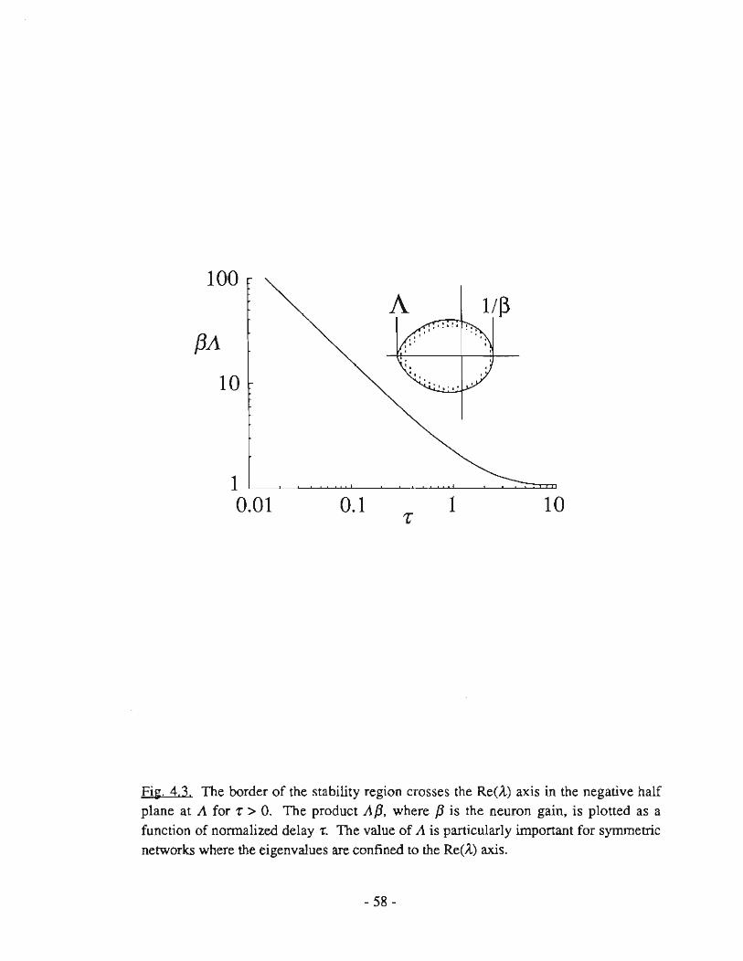
100
{JA
10
1 0.01 0.1
A 1//3
1 10
Fit:. 4.3. The border of the stability region crosses the Re(,l.,) axis in the negative half plane at J\. for 't" > O. The product 11./3, where /3 is the neuron gain, is plotted as a function of normalized delay 't". The value of J\. is particularly imponant for symmetric networks where the eigenvalues are confined to the Re(,l.,) axis.
- 58 -

solution as A, dropping the argument for the special case /1 = 1C. The value of A is
inversely proportional to the gain of the neurons and is a transcendental function of delay
defined implicitly by Eq. (4.13). A plot of the product 11./3, which depends only on
delay, is shown in Fig. 4.3. For large and small delay, A ean be approximated as an
explicit function of delay and gain:
~ (21C
T J T« I, (4.14a)
A -
1 1+(~J T» l. (4.14b) -/3 T+l
For a symmetri c connection matrix (Åi real) the origin will be unstable when
Åmax > 1//3 or Åmin < -A. The bifurcation at Åmax = 1//3 is a pitchfork (as it is
for T = O) corresponding to a single real root si of Eq. (4.6) passing inlo the half plane
Re(sj) > O. The bifurcation at Åmjn = -A corresponds to a Hopf bifurcation [Chaffee,
1971] of the origin, with a compIex pair of TOOtS si pas sin g inlo the half-plane
Re(si) > O at ±COi. The imaginary component COj = (/311. - 1)1/2 at the bifurcation
gives the approximate frequency of the oscillatory mode that resuIts from this bifurcation.
4.3.4. Symmetric networks with delay
Figure 4.4 shows the evolution of the stability region of the origin for a delay
network at three different values of gain. Each frame also shows schematically a
distribution of eigenvalues for one of two types of symmetric networks: The eigenvalues
on the left side of Fig. 4.4 are skewed negative, that is IÅmax/Åminl < I, while the
eigenvalues on the right side are skewed positive, with IÅmaxfÅminl > I. At low gain
- 59-

a
e
A ~<1 A max
I"" ',' ,,'
b
I, 'o'
f
Fig. 4.4. The stabil it y region of the origin and two different types of eigenvalue distributions (filled circles) are shown schematically. On the left (a,c,e), the eigenvalues satisfy IÅma .. /Åminl < l; on the right (b,d,f), the eigenvalues satisfy IÅma,,/Åminl > I. As the gain is increased, the stability region decreases in size and the origin loses stability. The bifurcations for each type of distribution are explained in the texl
- 60 -

(Figs. 4.4(a) and (b» all eigenvalues lie within the large stability region and the origin is
the unique fixed point and is stable. As the gain is increased, the size of the stability
region decreases as 1//3. The fust eigenvalue to leave the stability region will either be
the most negative, Amin, as in Fig. 4.4(c), or the most positive, Amax' as in Fig.
4.4(d). For the case in Fig. 4.4(d), a pair of attracting fixed points appear on either side
of the origin along the eigenvector associated with Amax and the origin becomes a
saddIe. For the case in Fig. 4.4(c), an oscillatory attractor exists along the eigenvector
associated with the eigenvalue Amin' The value of gain at which Amin leaves the
stability region in Fig. 4.4(c) is given by
/3 = (4. ISa)
where
w = - tan(w .. ) , (4.1Sb)
In the limit af small delay, this value of gain is
/3 = ( .. «l), (4.16)
and the period of oscillation is approximately 21r/w ( = 4rfor r« I).
For an eigenvalue distribution which satisfies IAmaxfAmin' < l, the first bifurcation
IO occur as the gain is increased can be either a pitchfork bifurcation, as Åmax leaves the
stability region, or a Hopf bifurcation as Åmln lea ves the stability region, depending on
the value of delay. For an eigenvalue distribution which satisfies lAmdAmin' > l ,
- 61 -

Åmat will always leave the stability region before Åmin regardless of delay.
A stability criterion for symmetric networks based on linear stability analysis can be
formulated by requiring that A.,nin' the minimum eigenvalue of Tij' remain inside of the
negative border of the stability region of the origin. In terms of the notation we have
defined, this eriterion requires -A < Amin' The condition can be simplified by noting
that A is always larger than its small-delay limit of 7r/(21:fJJ. The stability criterion for
symmetric networks with delay can thus be stated:
1: < 2 f3 Amin
::::) no sustained oscillation. (4.17)
This criterion lacks the rigor of a global stability condition, which exists for 1: = O
l Cohen and Grossberg, 1983; Hopfieid, 1984] and 1: 4 .., [Marcus and Westervelt,
1989c] but is supponed by considerable numerical and experimental evidence.
Figs. 4.4(e) and 4.4(f) show the situation when the gain is sufficiently large that
eigenvalues have left the stability region through both negative and positive borders,
indicating that Eq. (4.17) is violated and that fixed points exist away from the origin. In
thi s regime the system possesses multiple basins of attraction for coexisting fixed-point
and oscillatory attractors.
We find experimentally and numerically that delay networks in the large-gain regime
may or may not show sustained oscillation, depending on the value of delay and the
eigenvalue distribution. The observed behavior at large gain ean be c1assified aceording
to the ratio IAma.,/Aminl: Networks with IAmax/Aminl > l, as in Fig. 4.4(f), either do
not oscilIate at all or will oscilIate only when the delay is mueh larger than the relaxation
time. We have never observed sustained oscillation at 1: < l in any network satisfying
IAmax/Aminl > l experimentally or numerically. This result remains empirical, but is
consistent with the analysis in § 4.4 for delay networks that oscilIate coherently.
- 62-
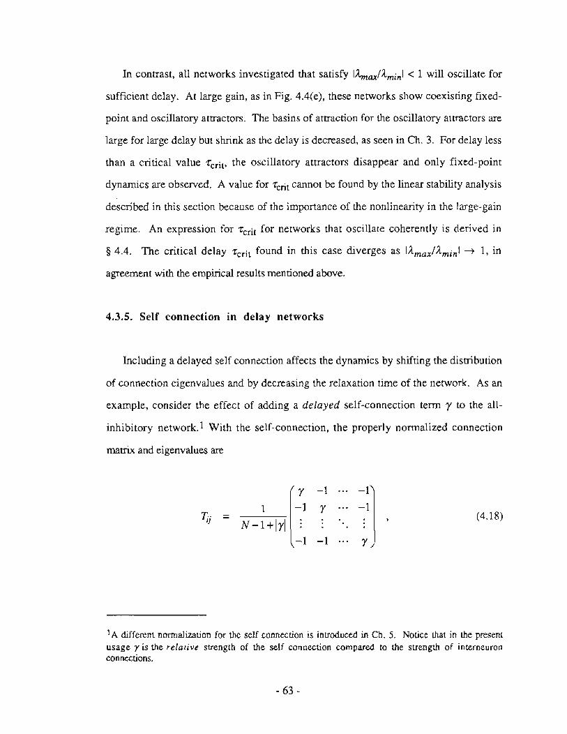
In contrast, all networks investigated that sarisfy lA",axlÅminl < l will oscillate for
sufficient delay. At large gain, as in Fig. 4.4(e), these networks show coexisring fixed-
point and oscilIatory attractors. The basins of attracrion for the oscillatory attraclOrs are
large for large delay but shrink as the delay is decreased, as seen in Ch. 3. For delay les s
than a crirical value -reri!, the oscillatory attractors disappear and only fixed-point
dynamics are observed. A value for -rerit canno! be found by the linear stability analysis
described in thi s section because of the importance of the nonlinearity in the large-gain
regime. An expression for -rerit for networks that oscilIate coherently is deri ved in
§ 4.4. The critical delay -rerit found in this case diverges as IÅmaxlÅminl -t l, in
agreement with the empirical results mentioned above.
4.3.5. SeIr connection in delay networks
Including a delayed seJf connection affects the dynamies by shifting the distribution
of connection eigenvalues and by decreasing the relaxation time of the network. As an
example, con sider the effect of adding a delayed self-connection term r to the all
inhibitory network.1 With the self-connection, the properJy normalized connection
matrix and eigenvalues are
r -l -l
l -I
N-l+lrl r -1
-1 -I r
(4.18)
1 A different nonnalization for the scl f eonnection is introdueed in Ch. 5. Notiec that in the present usage r is the re/ali ve strength of the self eonnection compared to the strength of int.emeuron connections.
- 63-

l+r [(N -I) - fold degenerate] N-l+lrI
Aj = (4.19)
l-N+r [once] .
N-l+lrI
The connection eigenvalues Amax and A",in for the all-inhibitory network are shown as
functions of the self-connection r in Fig. 4.5. Notice that adding a negative self
connection (r< O) does not change A"un' thus the value of delay where the Hopf
bifurcation occurs in the all-inhibitory network is not changed by a negative self
connection. Adding a positive self-connection (r> O) will bring Amin closer to zero
and will increase the delay necessary for the Hopf bifurcation to occur. The condition
IAmdAminl> l is satisfied in (4.19) when r exceeds (N/2 - l).
4.4. CRITICAL DELA y IN THE LARGE-GAIN LIMIT
In this section, we find a critical delay for sustained oscillation in the large-gain
regime, where fixed point attractors away from the origin coexist with a single coherent
oscillatory attractor. The main result, Eq. (4.23), applies to networks in which the
oscillatory attractor is along a coherent direction. Coherence is defined by the condition
that all IUil are equal. Equivalently, a coherent oscillatory attractor lies along avector
extending from the origin to any corner of an N dimensional hypercube centered at the
origin. When the eigenvector associated with Amin is in a coherent direction, then the
most robust oscillatory mode - that is, the one that will exist at the sma11est delay - will be
coherent. In this case, the network will not oscillate when the delay is smaller than the
critical delay derived below. Connection topologies which have a coherent direction
associated with Amin include all fully frustrated networks: the all-to-all, one- and two-
- 64 -

-1 1 y
-------------------f-1
Fi~. 4.5. The largest and smallest eigenvalues for the all·inhibitory network, Eq. (4.18), plotted as a function of the diagonal element y. The values indicated at the axis crossings are for a general N, but the scale of the drawing is correct for the case N = 3. The asymptotic value for all eigenvalues as y-+ ± 00 is ±l.
·65 -

dimensional inhibitory networks treated in § 4.5, as well as all Mattis transformations
[Manis, 1976] of these networks. For other networks discussed in § 4.5, including the
diluted inhibitory network and the negative-only c1ipped Hebb rule, the eigenvector
associated with Å"un appears numerically to approach coherence at large N, though this
has not been proven rigorously.
The stability criterion of § 4.3.4, stated as Eq. (4.17), applies at all values of gain but
becomes useless in the large-gain limit. In particular, Eq. (4.17) requires that the delay
go to zero as the gain diverges in order to prevent oscillation. Experimental and
numerical investigation suggest that this requirement is too severe, and that there is a
gain-independent critical delay "crit such that for .. < "crit sustained oscillation
disappears. Apparently, this critical delay resuIts from an instability of the oscillatory
attractor itself. Below, we derive a value for the critical delay "crit for coherent
oscillation in the large-gain limit by considering the stability of the oscillatory attractor.
This novel stability criterion agrees very well with experimental and numerical data.
4.4.1. Effective gain along the cuherent oscillatory attractur
The basic idea of the derivation is that neurons with saturating output can be regarded
as having an effective gain fJef! which is not constant as the state moves along the
oscillatory attractor, and ean be finite even when f(u) is infinitely steep at u = O. The
effective gain is defined as fJef! = f(u(t))/u(t). Note that fJeff is defined as the ratio
of the neuron output !(u(t» divided by the input u(t) which gave rise to that
particular output; this is a significant distinction for delay network, since the output
f(u(t» due to the input u(t) does not appear at the output until a delay time .. has
elapsed. This defmition of fJef! reduces to the usual gain fJ whenf(u) is linear (with
or without delay). We assume that the oscillatory attractor loses stability when the
- 66-

effective gain is sufficiently large at all points on along the attractor that perpenrucular
perturbations will always lead the system off of the attractor. This instability occurs
when the minimum value of f3ejf along the attractor exceeds a critical value related to
flow perpenrucular to the oscillation direction.
When the large-gain network is oscillating coherently. neuron outputs swing between
±l in Ihe form of a square wave. while the inputs altemately charge and discharge
exponentially with a time constant equal to the relaxation time of the network as shown in
Fig. 4.6(a). The smallest value of f3ett occurs when the input amplitude is at an
extremum of its charge-ruscharge oscillation and the corresponding output is saturated at
± 1. At this point. f3ett is the reciprocal of this input amplitude. The maximum
amplitude Ai al the l"lh input depends on the delay and is given by
(4.20)
For coherent oscillation along the direction associated with Åmin all of the Ai in Eq.
(4.20) will be the same (defined as A. with no subscript) and the term in the absolute
value of (4.20) will equal -Åmin (> O). In this case f3ejf will be bounded below by l/A.
as shown in Fig. 4.6(c):
l
A
l (4.21)
Flow perpendicular to the oscillatory attractor is described by Eq. (4.5) with the Åi
(i = J •. ..• (N-l)) equal to the N-J eigenvalues of T ij excluding Åmin and with
f3 = f3ett· The leas t stable of the N -l directions perpendicular to the oscillatory
attractor is along the eigenvector associated with Åmar. Thus the oscillatory attractor will
- 67 -

Fjg. 4.6. (a) The input u(r) (triangular wave) and output !(u(r-'t')) (square wave) for a sarurating infinite-gain neuron with delay in an oscillatory state. The value A. given by Eq. (4.20). is the maximum amplitude of the input. (b) The same input and output waveforms as above with the offset between input and output due to delay suppressed. (c) The effective gain 13e!!. defined as the ratio of !(u(r»/u(r), takes on finite values even when f(u) is infinitely steep at u = O. The minimum value of 13effis where the input is an exttemum; at this point 13eff= l/A. (d) The input and output of a delayed neuron from the electtonic circuit (Ch. 3) in a state of sustained coherent oscillation. Compare this to the idealized form in used in (a).
- 68 -
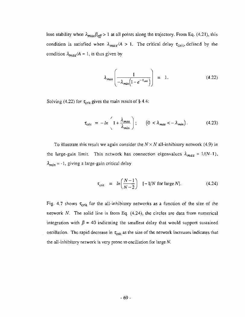
lose stability when Amaxf3eff> l at all points along the trajectory. From Eq. (4.21), this
condition is satisfied when Åmax/A > 1. The critical delay "erit, defined by the
condition Åmax/A = l, is thus given by
(4.22)
Solving (4.22) for "erit gives the main result of § 4.4:
= -In (1 + Å~ ) ; A.m",
(4.23)
To illustrate this result we again con sider the N x N all-inhibitory network (4.9) in
the large-gain limit. This network has connection eigenvalues Åmax = l/eN -1),
Amin = -1, giving a large-gain critical delay
't'crit = ln(~) N-2
[-ljN for large N]. (4.24)
Fig. 4.7 shows "erit for the all-inhibitory networks as a function of the size of the
network N. The solid line is from Eq. (4.24), the circles are data from numerical
integration with f3 = 40 indicating the smallest delay that would support sustained
oscillation. The rapid decrease in "erit as the size of the network increases indicates that
the alJ-inhibitory network is very prone to oscillation for large N.
- 69-

1
0.1
0.01 1
FIXED POINTS ONLY
10
FIXED POINTS AND SUSTAINED OSCILLATION
N 100
Fig. 4.7. Large-gain eriticai delay -rerit for the all-inhibitory network plotted against N,
the size of the network. Solid curve is the theory from Eq. (4.23), the filled circles are from numerical integration of the delay equations at f3 = 40. Numerical integration data were ob tai ned by starting the system with initial functions Ød --r,0] along the eigenvector associated with Amin and constant over the time interval r --r,0]. The delaydifferential equations were integrated using a modified Euler method: A stack of IO - 40 previous states was maintained for each neuron. Upon each Euler step, the elements in the stack were moved down one position and a new state was added to the top of the stack. The step size and size of the stack were chosen so that a state reached the bottom of the stack at precisely the specified delay, and could then be used as the neuron's delayed output. The system was checked for oscillation af ter many (up to I(4) time constants. The critical delay was found by repeating the integration using a IO-split binary search in the value of delay.
-70 -

4.4.2. Crossover from low gain to high gain regime
We have now found two critical values af delay: For small gain (13 < Åmax) the
network does not oscillate for, < TH, where T:H is the value af delay where the Hopf
bifurcation occurs. For small delay,
(4.25)
At large gain, the delay network does not oscilIate for T: < Terit, where Terit is given
by Eq. (4.23). We now ean sider the erossover from the small-gain regime to the large
gain regime for the speeifie example af an all-inhibitory triangle af neurons. For this
network,
-I] -1 ;
O
, _ 1 I\..max -2 Åmin = -1. (4.26)
Fig. 4.8(a) shows the two theoretical eurves for eaeh of the two regimes. The data
points are the values af delay where the oscillatory attraetor disappears as measured in the
analog circuit (op en eirc1es) and by numerically integrating the delay equations (filled
eirc1es). Fig. 4.8(b) shows four regions af the 13 - T plane, each with distinct
dynamical properties. For 13 < 2 and T < TH, where 'H is found by setting Åmin = -1
in Eq. (4.15), there is a single fixed point attractor atthe origin. For 13 < 2, T> 'H,
the fixed point at the origin is unstable and there is a single oscillatory attractor. At 13 =
2 fixed points away from the origin appear. At this crossover point, T:j{ ;: 1.209. For
13 > 2, the Hopf bifurcation line no longer marks the critical delay for sustained
- 71 -

10 , :rH (a)
r 1 • t T cril
• \ • "
0.1 L-._~~~~~,-_~~~_........J 1 10
f3 100
10
0, (b)
\ OM
~
S, SM
0.1 1 10 f3 100
Fig. 4.8. Phase diagram for the all-inhibitory (or frustrated) triangle of delay neurons. (a) Two theoretical curves are shown. The curve labelled TH indicates the value of delay and gain where the origin undergoes a Hopf bifurcation, from Eq. (4.17); the line labelled Terit indicates the large-gain critical delay where the oscillalOry mode 10ses stability. For T < Terit only fixed-point attractors are stable. The data points are critical delays measured in the electronic network (open circles) and by numerical integration (fIlled circles) with f3 = 40. Numerical integration data were obtained as described in the caption of Fig. 4.7. (b) The four regions in the f3 - T plane with qualitatively different dynamics are: S l: Single fixed point attractor at the origin; Ol: Single coherent oscillatory attractor; SM: Multiple fixed point attractors away from the origin, all fixed points; OM: Multiple attractors away from the origin, including ftxed points and a coherent oscillatory attractor.
-72 -

oscillation. As f3 becomes large, the erirical delay for sustained oscillation approaehes
the gain-independent theoreticaI value of 'l"crit. From Eq. (4.24), 'l"crit(N=3) = ln(2)
== 0.693.
4.5. STABILITY OF PARTICULAR NETWORK CONFIGURATIONS
In [his section we consider sustained oscillation in fOUT symmetrie delay networks:
(1) symmetrically connected inhibitory rings; (2) large two-dimensional arrays of nearest
neighbor lateral inhibition networks on square and hexagonallattices; (3) spin-glass-like
random symmetric networks; and (4) Hebb rule and c1ipped Hebb rule associative
memories.
4.5.1. Symmetrically connected rings
A ring of neurons with symmetric connections, all of equal strength but of either
sign, inhibitory or excitatory, has a spectrum of connection eigenvalues given by
Ak = cos(2; (k+rp)) k=O,I, ... ,(N-l). (4.27)
where II' = 1/2 for a frustrated ring, i.e. Sgn(llring Tij) = -1, and II' = O for a
nonfrustrated ring [Reger and Binder, 1985]. (The normalized matrix has elements
T ij = Tji = ±1/2.) The ratio of maximum to minimum eigenvalues can be found
directly from Eq. (4.27):
- 73-

cos(n/N) [< l] N odd; frustrated,
~ Åmin sec( n/N) [> I] N odd; nonfrustrated, (4.28)
I N even; frustrated or nonfrustrated.
Notice that only frustrated rings with odd N satisfy the condition I).",aJAminl < l,
suggesting that only these configurations will show sustained oscillation. This
conclusion is confIrmed experimentally and numerically. The large-gain critical delay for
the frustrated ring with odd N is found from Eq. (4.23),
(N odd, frustrated). (4.29)
Notice also that Tcril increases with increasing N for the symmetric ring, while for the
all-inhibitory network Teril decreases with increasing N. Inhibitory rings are thus much
less prone to oscillation than fully-connected inhibitory networks. The eritical delays
from numerical integration are compared to Eq. (4.29) in Fig. 4.9.
-74 -

3.0 D large-gain theory
• numerical integration
2.0 iii
1.0 Il
O. O '-------L_...l......----'-_---'-_ L----L_-'----'_---'------'
O 1 2 3 4 5
N
6 7 8 9 10
Fil:. 4.9. Large-gain critical delay Terit for symmetrically connected frustrated rings with N = 3,5,7,9 from Eq. (4.23) (open squares) is plotted along with crirical delay from numerical integration (filled circles) with f3 = 40. Numerical integration data were obtained as described in the caprion ofFig. 4.7. Frustrated symmetric rings with even N do not satisfy I ÅmaxlÅmin I < 1 and therefore are not expected to oscilIate for any delay within the large-gain theory. Numerically, frustrated rings with even N showed sustained oscillation only for very large delay (T> 10), though this is possibly a numerical artifact
- 75 -

4.5.2 Two-dimensional lateral-inhibition networks
An important network configuration, especially IO the study of real and artificial
visual systems, is one in which each neuron inhibits the activity of its neighbors. This
configuration, called lateral inhibition, is ubiquitous in vertebrate and invertebrate vision
systems [Dowling, 1987], and is widely used in artificial vision systems for edge and
feature detection. Lateral inhibition has also been incorporated into an e!ectronic VLSI
modelof the retina [Mead, 1989]. The function of lateral inhibition is to enhance the
contrast of edges in a visual scene [RatIiff, 1965; Dowling, 1987] and to broaden the
dynamic range of a visual system by setting a local rather than global reference point for
measuring relative intensity variations [Mead, 1989].
A case of lateral inhibition in which time delay is significant is in the compound eye
ofthe horseshoe crab, Limulus [for a collection ofpapers see: Radiff, 1974]. It is found
experimentally that the individual eyelets (ommatidia) that form the compound eye of
Limulus are mutually inhibitory, and that there is a significant time delay (- 0.1 sec.)
before lateral inhibition is activated between any pair of ommatidia. It is also found that
under certain experimental conditions, a spatially uniform illumination over the entire eye
will induce sustained coherent oscillation, with all ommatidia showing an in-phase
periodic modulation in their output firing rate, with aperiod of - 0.3 sec. [Barlow and
Fraioli, 1978].
Such experiments have stimulated several mathematical analyses addressing
oscillation in delayed lateral inhibition systems [Coleman and Renninger, 1974, 1975,
1978; Hadeler and Tomiuk, 1977, an der Heiden, 1980]. These analyses have assumed
uniform, all-to-all coupling between ommatidia, and further have assumed a coherent
form for the oscillatory solution, which allows the problem to be reduced to a one
dimensional de1ay-differential equation for motion along the in-phase (1,1, ... ,1)
- 76-

direction. This second assumption dees not allow an instability of the oscillatory mode to
broken-symmetry states, and thus previous treatments have not predicted the instability of
the coherent oscillatory solution which lead to our large-gain critical delay "l"crit in § 4.4.
Already in Ch. 4 we have considered two extremes of lateral inhibition networks: the
all-to-all inhibitory network (Eq. (4.9) and (4.24)) and the one-dimensional laterally
inhibiting ring, which is covered by the analysis in § 4.5.1. These two networks are
seen to behave quite differentlyas the number of neurons becomes large. Specifically, as
N ~ ~ the eritical delay "l"crit from (4.23) tends to zero for the all-to-all inhibitory
network and tends to infinit y for the one-dimensional ring with nearest-neighbor
inhibition (for now, we set the self-eonnection y= O):
"l"cri' ~ O as N ~ ~ (all-to-all),
rcrit ~ ~ as N ~ ~ (l -D ring).
(4.30)
(4.31)
Of course, the case of most direct application to vision is neither of these extremes, but
rather a large 2-D network. In this subsection, we show that the stabil it y of large 2-0
networks with delayed nearest-neighbor lateral inhibition depends crucially on the form
of the lattice. With the neurons on a square lattice (Fig.4.1O(a», we find
"l"crit ~ ~ as N ~ ~ (2-D square lattice). (4.31)
That is, this configuration will not show sustained oscillation in the large-N limit. In
contrast, when the neurons are placed on a triangular lattice (Fig. 4.1O(b» the critical
delay for sustained oscillation isfinite in the large-N limit, approaching the limit
rcril ~ In(2) = 0.693. .. as N ~ ~ (2-D triangular lattice). (4.32)
- 77-

- -Ca)
! J
)
( '- v
(b)
Fig. 4.10. Two-dimensional lattices with lateral inhibition. (a) Square lattice, (b) triangular lattice.
- 78 -

For generality, we introduce a diagonal element y in the connection matrix (before
normalization), corresponding to a delayed self-inhibition (r< O) or self-excitation
(r> O). The value of r indicates relative strength of the delayed self-connection
compared to the strength of the delayed lateral inhibition (as used in Eq. (4.18)). With
the delayed self-connection r. the crirical delay for the 2-D triangular lalrice becomes
( r-6 ) 'l" crit -t In as N -t "".
2r- 3 (4.33)
We restrict the r to the range -3 < r< 6 to insure O < Åmax < - Åmin' which was
assumed in the analysis of § 4.4. Equation (4.33) indieates that the triangular lanice ean
oscilIate even when there is an overall self-exeitation, as Ion g as y< 1.5.
It rnay seem surprising at first that the type of latrice ean so greatly affect the network
dynamies. The key to understanding the difference is realizing that on the triangular
lattice, lateral inhibition (or, equivalently, antiferromagnetism) isjrusrrared, but on the
square lattice it is nol. On the square latrice, in faet, lateral inhibition is exaetly equivalent
to lateral excitation via a Mattis transformation [Mattis, 1976). This difference is also
seen in 2-D magnetic models: While ferrornagnets on square and triangular lanices behave
nearly identically (both are nonfrustrated), the corresponding 2-D antiferromagnets are
quite different, due to the presence of frustration in the triangular lattice, but not the
square lattice [Wannier, 1950). As diseussed in § 4.3.2, the presence of frusITation
seerns to be essential for a delay network to support sustained oscillation.
To derive the above results, Eqs. (4.31)-(4.33), we need the eXITemal eigenvalues of
the connection matrix for nearest-neighbor inhibition on these 2-D lattices. The value of
'l"crit ean then be found immediately from Eq. (4.23). This sort of eigenvalue problem
is frequently encountered in eondensed matter physics, for example to describe the
-79 -

vibrational modes of a 2-D lanice2. Therefore, the eigenvalue spectra will be presented
without derivation (see, for example [Ashcroft and Mermin, 1976, Ch. 22]). We assume
periodic boundary conditions and take NI and N 2 as the number of neurons along each
of the two lattice veClors. (The total numbeT of neurons is the product N IN2') As
usual, Ihe connection matrix obeys the normalization "Ej ITi} = 1. The eigenvalues
Åk""" of Tij, for the 2-D square lanice are given by
y- 2[ cos(2nkJ! Nd + cos(27rk2/N2) J IYl+ 4
(4.34)
where the indices range over the values kI,2 = 0,1, ... , (NI,2-1). From (4.34), we find
that for the square lanice, the ratio appearing in (4.23) limits to
y+4 = y-4
(4.35)
To apply the analysis of § 4.4.1, which assumed ° < Åma;c < - Åmin' we require
-4 < y< 4. From (4.35) and (4.23) we conclude thai for y ~ 0, ~cril .-,00 for large
2-D square lanices, as NJ,N2 '-'00.
The eigenval ues for the triangular lattice are given by
Åkk(r)= l , 2 IJ
y - 2[ coS(27rkdNJ) + cos(27rI0./N2) + cos(2tr(kJ/NJ - k2/N2 l)] IYl+ 6
where, again k1,2 = 0,1, ... , (NI ,2-I). In this case, the ratio in (4.23) limits to
2A very heIpful discussion wi!h R. D. Mcadc regarding !his point is gralefulIy acknowledged.
- 80-
(4.36)
(4.37)

and we require -3 < Y < 6 to insure O < Amax < - Amin' Notice that for the triangular
lattice,
(4.38)
for y < 1.5. Equations (4.38) and (4.23) indicate that a nearest-neighbor lateral
inhibition network on a large triangular lattice has a finite value for -rerit as long as the
(delayed) self-excitation strength remains les s than 1.5 times the lateral-inhibition
strength. From (4.37) and (4.23), we ean find the value of -rerit given above in Eqs.
(4.32) and (4.33).
The eigenmode associated with the most negative eigenvalue of (4.36) is k l = O,
k2 = O. This O-wavevector mode is the in-ph ase (coherent) direction in state space, as
shown in Fig. 4.11(a), which justifies the application of the large gain analysis and Eq.
(4.23). Further consideration reveals that the mode associated with the most positive
eigenvalue - the mode which first goes unstable IO break the symmetry of the coherent
oscillation - is the -v'3 x-v'3 mode shown in Fig. 4.11(b).
- 81 -

t-+-t-t
(a) /\/\/\/\ t-t-t-t-+
/\/\/\/\/\ t-t-t-t-t-t
/\/\/\/\/\/\ t - t-t-t-t-t-t
\/\/\/\/\/\/ t-t-t-+-+-t
\/\/\/\/\/ t-t-t-t-t
\/\/\/\/ +-t-t-t
+-0---+
/\/\/\/\ (b) 0---+-0--
/\/\/\/\/\ --t-O---+-O
/\/\/\/\/\/\ t-O---t-O---t
\/\/\/\/\/\/ --t-O---t-O
\/\/\/\/\/ O---t-O--
\ /\/\/\/ t-O---t
Fig. 4.11 . Eigenmodes associated with the extremal eigenvalues of Tij for the triangular lateral inhibition network, from Eq. (4.36). (a) The mode associated with Åmin is the coherent, in-phase mode, k l = k2= O. This is the oscillatory mode which appears for
the smallest value of delay. (b) The mode associated with Åmar is a .f3 x.f3 structure. The wave vectors for this mode are at the vertices of the hexagonal Brillouin zone. This is the fIrst mode to break the symmetry of the coherent oscilIatory mode, giving the value
for "eri!"
- 82-

4.5.3. Random nelworks
Sustained osciJlations in randOInly connected neural networks have been considered
previously for symmetric networks with parallel dynamics [Cabasino et al.,1988] ,
which show at most period-2 oscillation s [Peretto, 1984; Goles-Chacc et al., 1985;
Goles and Vichniac, 1986; Grinstein et al., 1985; Frumkin and Moses, 1986; Marcus
and Westervelt, 1989c] and for asymmetric networks with parallel dynamics [Amari,
1971; Shinomoto, 1986; Gutfreund et al., 1988; Klinen, 1988], sequential dynamics
[Shinomoto, 1986; Gutfreund et al., 1988] , and continuous-time dynamics [Amari,
1972; KUrten and Clark, 1986]. Periodic as well as chaotic dynamics in a mean field
spin-glass model with delayed interaction have also been described [Choi and Huberman,
1983b].
We will only con sider the effect of delay in symmetric random networks, and we
find only simple (non-chaotic) oscillation above a critical delay. The absence of chaos in
the symmetric cominuous-time delay network (with monotonic nonlinearity) is not
surprising, as the two limits of short and long delay are known to possess only fixed
points and period-2 oscillations: A rigorous proof of this conjecture for the general delay
differential system has not been presented to our knowledge.
We consider a delay network with symmetric connection matrices whose elements
Tij (= Tji ) are independently fixed at one of three values (+,-,0). Any two neurons are
connected by a positive connection with probability p+ and by a negative connection
with probability PO' The connectance p is defined as p = (p+ + p.); the bias q is
defined as q = (p+ - p.). The normalized matrix T iJ' has elements
j±_l T;j = Tji = pN
° with probability P±
(4.39)
with probability 1- p.
- 83-

The eigenvalue specuum of a random symmetric matrix is described by the famous
Wigner semicircular Jaw [Wigner, 1958; Edwards and Jones, 1976] (For a generaJization
of the semicircuJar law to random asymmetric matrices, see [Sommers et al.,1988]).
The notation used here follows Edwards and Jones [19761. For an N x N random
symmetric matrix whose elements have a mean M O/N and a variance a2/N, the
spectrum of eigenvalues p(Å) converges for large N to a continuous semicircular
distribution. For MO = O,
and for M o ~ O,
For the (+,-,0) matrix, Eq. (4.39), we identify
q Mo H
p
IÅI<2a
IÅI> 2a
(4.40a)
(4.40b)
(4.4la)
(4.4 Ib)
From Eq. (4.40) and Eq. (4.41), we can find the maximum and minimum eigenvalues of
- 84-

Tij- Setting Ti; = O adds a tenn of O(l/N) IO all of the eigenvalues; we will neglect
this and all tenns O(l/N). These resulls are therefore valid only for large N, where
NI/2 «N.
2 ~p-l O(~) forq<~ - + P N
Å = (4.42a) max
q + O(~ ) forq>~
p
_3..~Jl-l + O(~) for -q<~ Åmm = Jl N
(4.42b)
2.. + O(~) for -q>~ p
The condition lA.max/Åminl < l is only satisfied when -q > (P/N) 1/2, suggesting that a
symmetric random network must be biased sufficiently negative before it will oscilIate for
small delay ( "' < - 1).
4.5.4. Random symmetric dilution of the all-inhibitory network
An example of a random symmetric network that will oscilIate for small delay is the
randomly diluted inhibitory network. For this network Jl+ = O and p = -q = p_. To
O(I/N), the maximum and minimum eigenvalues are
Å = max ~ (..!.. _1)V2 'li ' "V IV p_
(4.43a)
Åmm = -I. (4.43b)
- 85 -

Fig. 4.12. The range of connection eigenvalues for asymmetricaIly diluted inhibitory network with N=100 from Eqs. (4.40) and (4.41) is plotted as a function of the connectance p_ (solid curves). The line at Å = -1 indicates a single eigenvalue Åmin
Iying outside of the quasi-continuous distribution. The smaIl crosses are eigenvalues
computed for randomly generated symmetric 100 x 100 matrices with p. = 0.4, 0.7, and 0.9.
- 86-

Fig. 4.12 shows the Iheoreticai range of eigenvalues for a 100 x 100 randomly diluted
inhibitory matrix as a function of connectance p_o The small crosses are the eigenvalues
of computer-generated random (-,O) matrices with p. = 0.4, 0.7 and 0.9.
For the randomly dilUled inhibitory network, with or without delay, the neuron gain
at which the origin becomes unstable via a pitchfork bifurcation, creating fixed points
away from Ihe origin, is given by
{3= -fN(~_IJ-1/2 2 p_
(pitchfork). (4.44)
Because il."un is independent of connectance, Ihe delay at which the origin loses stability
by a Hopf bifurcation is also independent of connectance. Inserting Amin = -1 into
Eq. (4.25) gives 1:H == ;r/2{3, the small-delay limit being appropriate for large N and
therefore large {3.
The large-gain analysis of § 4.4 can be applied to the diluted inhibitory network when
N is large. At large N the eigenvector associated with Amin is nearly coherent, that is,
the differences in lUi' along the eigenvector associated with il."un are small compared to
IUil and appear numerically to vanish as N -t "". Applying Eq. (4.23) gives a gain
independent critical delay which depends on the connectance. From Eq. (4.23) and Eq.
(4.43), the randomly diluted inhibitory network will not oscillate in the large-gain limit
for 1: < "eri! ' where
(4.45)
Fig. 4.13 shows 1:cri! as a function of connectance p_ for N = 1000. (At p_= l, the
- 87 -

result from Eq. (4.24) is used instead ofEq. (4.45) which neglects telTIls ofG(I/N) and
is therefore not valid precisely atp_= 1.) Figure 4.13 shows that for a very mild dilution
of connections, 1:cril is greatly increased, but addition al dilution does little to increase
1:cril funher. When the dilution d'" (1- p_l is mild (d « l), the right hand side of
Eq. (4.45) ean be expanded to yield
(N-1 « d « l). (4.46)
Eq. (4.46) can be compared to the erirical delay for the undiluted a11-inhibitory network,
Eq. (4.24), to give a simple expression for the increase in critical delay due to random
symmetric dilurion:
1:(diluted) cnt
'r(~di1utcd) -ent
(4.47)
This result demonstrates how small random dilution of a large inhibitory network ean be
used to stabilize a network by increasing the crirical delay for sustained oscillation.
- 88-

1
0.1
'l' . eTlt
0.Q1
N=iOOO
0.001 ~----~------~------~----~----~ O 0.2 0.4 0.6 0.8 1.0
Fi~. 4.13. Plot of the large-gain critical delay "crit as a function of connectance p_ for the diluted inhibitory network with N = 1000. Note that very mild dilution greatly increases "crit. At the point p_ = l the result of Eq. (4.24) is used instead of Eq. (4.45) which neglects tenns of OO/N), and is not correct at p_ = l.
- 89-
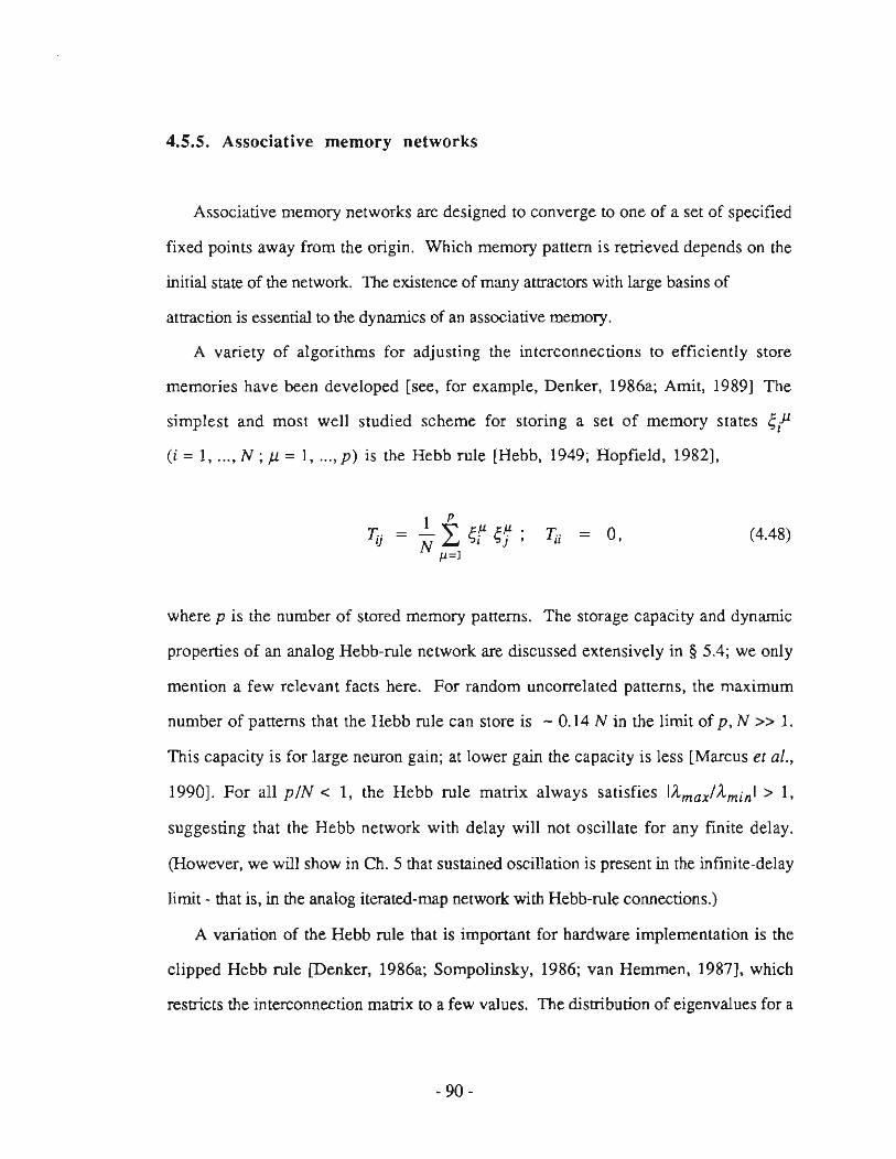
4.5.5. Associative memory networks
Associative memory networks are designed to converge to one of a set of specified
fixed points away from the origin. Which memory pattem is retrieved depends on the
initial state of the network. The existence of marry attractors with large basins of
attraction is essentialto the dynamics of an associative memory.
A variety of algorithms for adjusling the interconnections IO efficiently store
memories have been developed [see, for example, Denker, 1986a; Amit, 19891 The
simplest and most well studied scheme for storing a set of memory states ~,Jl
(i = l, ... , N; J.l = l, .. . , p) is the Hebb rule [Hebb, 1949; Hopfieid, 1982],
Iii = 0, (4.48)
where p is the number of stored memory pattems. The storage capacity and dynamie
properties of an analog Hebb-rule network are discussed extensively in § 5.4; we only
mention a few relevant facts here. For random uncorrelated patterns, the maximum
number of pattems that the Hebb rule ean store is - 0.14 N in the limit of p, N » 1.
This capacity is for large neuron gain; at lower gain the capacity is les s [Marcus et al.,
1990). For all pIN < l, the Hebb rule matrix always satisfies IAmaxlAminl > l,
suggesting that the Hebb network with delay will not oscilIate for any finite delay.
(However, we will show in Ch. 5 that sustained oscillation is present in the infinite-delay
limit - that is, in the analog iterated-rnap network with Hebb-rule connections.)
A variation of the Hebb rule that is important for hardware implementation is the
clipped Hebb rule [Denker, 1986a; Sompolinsky, 1986; van Hemmen, 1987], which
restricts the interconnection matrix to a few values. The distribution of eigenvalues for a
- 90-

clipped Hebb matrix Ti/ is greatly affected by the detail s of the clipping algorithm as
seen in the numerical data of Fig. 4.14. Fig. 4.14(a) shows the distinct eigenvalues
Å(Tij") for the clipping algorithm Tij" = (I/Z)Sgn(T ij ). where Z is the
normalization Z = LiISgn(Tij)l. This clipping algorithm introduces large negative
eigenvalues but still satisfies IÅmax/Åminl > l for all values observed of p. We
conclude that networks built with this c1ipping algorithm will not oscilIate as long as the
delay is not mueh longer than the relaxation time - to be safe. when 1: < - 1.
Experimentally (in the electronic circuit) and numerically. we find that this c1ipping
algorithm does not produee sustained oscillation until the delay is much longer than the
relaxation time (1:» 1). Fig. 4.14(b) shows the distinct eigenvalues for the negative
only clipping algorilhm: -Ti/* = (l/Z)(J(-Tij)' where 8 is the Heaviside function and
Z = Li 8(-Tij)' This clipping algorithm. whieh sets all positive elements of the
unclipped matrix T ij to O and all negative elements IO -l/Z. has the hardware advantage
af only requiring a single inverting output from each neuron. as pointed out by Denker
[1986b]. As seen in Fig. 4.14(b). Ihis algorithm unfortunately introduces a large
negative eigenvalue whieh ean lead to sustained oscillation for a neuron delay of the order
ofthe relaxation time (1:<-1).
4.6. CHAOS IN TIME-DELA Y NEURAL NETWORKS
4.6.1. Chaos in neural network models
Relaxing the constraint of symmetric connections greatly enriches the repertoire of
neura! nelwork dynamics and provides powerful computational properties that are not
available in symrnetric networks. The most important novel feature of asymmetric
networks (with or without delay) is that attractors need not be fixed points. Depending
on the details of the connection matrix and the network dynamics. the attractors in
- 91 -
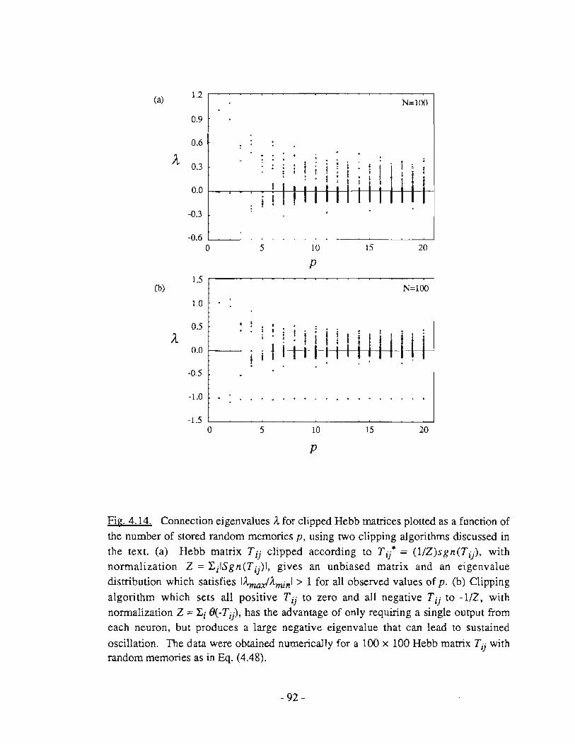
(a) 1.2
N=l00
0.9
0.6
A 0.3
0.0
-0.3
-0.6 O 5 10 15 20
P 1.5
(b) N=IOO
1.0
0.5 • ! , i • i I .
i I , , H+ A ! I I
I I I I I 0.0 IH I I I I I ! -0.5
-1.0 . . . .
-1.5 O S IO 15 20
P
Fig, 4.14. Connection eigenvalues ).. for clipped Hebb matrices plotted as a function of the number of stored random memories p, using two clipping algorithms discussed in the tex!. (a) Hebb matrix Tij clipped according to Ti/ = (l/Z)sgn(Tij), with normalization Z = LjISgn(Tij)l, gives an unbiased matrix and an eigenvalue distribution which satisfies I)..ma.r')..minl > 1 for all observed values of p. (b) Clipping algorithm which sets all positive Tij to zero and all negative T jj to -liZ, with normalization Z = Lj O(-Tj}, has the advantage of only requiring a single output from each neuron, but produces a large negative eigenvalue that can lead to sustained
oscillation. The data were obtained numericaIly for a 100 x 100 Hebb matrix T ij with random memories as in Eq. (4.48).
- 92-
asymmetric networks may be periodic or chaotic.
Chaos is usually taken to mean quasi-random behavior in a deterministic dynamical
system [Guckenheimer and Holmes, 1983; Berge er al., 1984]. TypicalIy, though not
always, the dynamicaI system of interest is 10w dimensional. This is, of course, not the
case for de1ay systems [see, for examp1e: Farmer, 1982] or for neural networks with
large N. The term "chaotic" is used both to describe a dynamical system (perhaps with a
panicu1ar set of parameter values) or to describe an artractor of a dynarnical system. The
distinction is a erucial one, however, sinee a chaotic attractor may occupy only a smaII
volume of the system's state space. Chaotie and non-chaotic attraetors often eoexist in
state space, each attractor having its own basin of attraction. This can make the presence
of ehaos in a high-dimensional system (such as a neural network) difficuIt to detect, sinee
a panicular set of inilial conditions may, for example, lead to a fixed point, while a
nearby chaotic attraclor remains undetected.
A definitive signalure of a ehaotie attractor is sensitivity IO initial eondilions, whieh
means that c!ose-lying points on the attraetor move away from each olher as time evolves
(for short times). In large random dynamieal systems the corresponding signature of
chaos is the vanishing of an average autocorrelation function [Sompolinsky et al.,
1988).
A. Chaos in large asymmerric networks
Chaos in large delenninistic neural networks with random asymmetric conneetions
has been studied extensively in several network models [Kiirten and Clark, 1986;
Shinomoto, 1986; Derrida, 1988a; Kiirten, 1988; Sompolinsky, et al., 1988; GUlfreund,
et al. , 1988; Bauer and Martienssen, 1989; Spitzner and Kinze1, 1989; Renals and
Rohwer, 1990). Unfortunalely, a consislent pieture of when and how ehaos arises from
random connections has nOl yet emerged.
- 93 -

Sompolinsky er al. [1988] considered the large-N behavior of a network of analog
neuron s with continuous-time dynamics. They found that when the connection matrix
elements are independent random variables with zero mean, and with zero correlations
between Tij and Tji , the only attractors (in the large-N limit) are: (l) the fixed point at
the origin for low neuron gain; and (2) a chaotic state above a critical value of gain.
Numerical evidence in support of this claim is given by Bauer and Martienssen [1989],
who also describe a transition to chaos via quasi-periodicity (see also [Renals and
Rohwer, 1990]). However, Gutfreund et al.[l988], in an investigation of small random
networks of binary neurons with discrete-time dynamics , found that long-period
attractors exist only when the connection matrix is completely asymmetric, but that
whenever there is a correlation between Tij and ~'i ' short -period attractors predominate.
This result suggests that the presence of chaos in large random networks is not so
common, being present only in fuIly asymmetri c networks. Spitzner and Kinzel [1989]
present numerical evidence to the contrary: They find that random networks of binary
neurons with parallel updating show a sharp transition from a so-called frozen state to a
chaotic state as a function of the correlation between Tij and Tji , and that the transition
to the chaotic state occurs at a non-zero value of the correlation. At the opposite extreme,
analyticai and numerical work of Crisanti and Sompolinsky [1987] for the asymmetric
spherical model (an approximation to analog neurons) suggests that as N ~ 00 all frozen
states disappear, leaving only chaos, as soon as an infinitesimal amount of asymmetry is
introduced into the connections .
Shinomoto [1986], extending early work by Amari (1971), considered the effect of
random connections for distributions of connection strengths with non-zero mean. Re
presents a numerically derived phase diagram showing that randomly connected binary
neurons with parallel updating are chaotic only when the mean of the distribution is
within a narrow range. For a large negative mean, only period-2 attractors are observed;
- 94-

for a positive mean, only fixed point attractors are observed.
An alternative approach to identifying chaos in large random asymmetric networks is
based on the sensitivity to initial conditions described above [Derrida, 1988a]. The idea
here is to follow the evolution of a statistically averaged distance between two initial
states and observe whether this distance converges or diverges under the dynamics of the
network. Derrida [1988a] treated a highly dilute asymmetric spin glass model in thi s
manner and idemified a transition to a chaotic phase, where pairs of initial conditions
always diverge, as the connectivity of the network is decreased. Klirten [1988] showed
that for dilute networks of binary neurons, Derrida's transition also marks a transition to
a phase in which the mean length of Jimit cycles grows exponemially with the size of the
system.
B. Chaos in small networks
Large system size is not necessary for the existence of chaos in neural networks.
This faet has been demonstrated for continuous-time analog networks by Kepier et
al .[1989] who used a 6-neuron elecrronic network with computer-controlled
interconnections to rapidly test many random matrices for chaotic dynamics. They found
that chaos was rare but present. They also identified some general characteristics of the
connection matrices that result in chaotic networks. Matrices leading to chaos tend to have
average loop correlations that obey the folIowing trends: (TijTji ) < O; (TijTjkT/d) - O;
(TijTjkT/<mTmi»O. Babcock and Westervelt [1986a ;1986b] have shown that a simple
analog network of two neurons with an inductive component in the coupling ean become
chaotic when driven by an oscillating external current.
C. Chaos in time delay networks
Neural networks with nonsymrnetric connections and time delay can be configured as
- 95-

associative memories for the storage and recaU of sequences of patterns. These networks
have been described and studied by a number of researchers [Grossberg, 1970;
Kleinfeld, 1986; Somplinsky and Kanter 1986; Gutfreund and Mezard, 1988; Riedel,
et al., 1988; Herz, et al., 1988; Kiihn, et al., 1989]. It has been show n that for cenain
parameter values, these large sequence-generating networks can also be chaos-generating
[Riedel, 1988]. Chaos in scalar delay-differential systems will be discussed in § 4.6.3.
4.6.2. Chaos in a small network with a single time delay
The electronic analog network described in Ch. 3 shows endogenous chaos for
particular connection configurations and network parameters. We now describe one such
example using three neuron s, one with delay. The dynamical equations for the chaotic
network are
Cj Uj(c') = - ~ . Uj(t') + I
N
L Ii; f j (uk - rj)) , j=1
j = 1,2,3. (4.49a)
where
T .,=_I_ l
[
O
l} 105 .Q 1 (4.49b)
Ri = (l:J'T'iJ')·I, and C 1= C2 = C3 = 10nF. The characteristic relaxation times for
the three neuron s (in the absence of any delay) are RICI = O. Sms , R2C2 = l. Oms ,
R3C3 = 1. Oms. The neuron transfer functions are well-approximated by tanh functions
with the folIowing gains and amplitudes:
- 96-

Only neuron l is delayed,
li (u) = 3.8tanh(8.0u),
!z(u) = 2.0tanh(6.1u),
h (u) = 3.5tanh(2.5u),
",' = ro "1 - 1
(4.49c)
(4.49d)
The outputs of neurons 1 and 2 are shown in Fig. 4.15 for four values of the delay 1"
ranging from 0.64 ms to 0.97 ms. For 1" < 0.64 ms the system shows limit cyc1e
behavior similar to that shown in Fig. 4.15(a). In the range 1" = 0.64 ms - 0.97 ms
the system undergoes a series of period doubling bifurcations leading to chaos. As the
delay is increased beyond 0.97 ms, both chaotic and periodie regimes are found.
4.6.3. Chaos in delay systems with noninvertible feedback
The chaotic circuit described above is c10sely related to a well-studied class of chaotic
de1ay-differential systems with noninvertibie feedback [see, for example: Mackey and
Glass, 1977; Farmer, 1982]. These systems are defined by a scalar de1ay-differential
equation of the form
x(t) = -ax(t) + h(x(t - 1")) , (4.50)
where a,1" > O, and the function h is noninvertible (also called "humped" or "mixed").
Equation (4.50) has been studied in the context of white blood-cell production
- 97 -

! "C~O.64ms l 1"C~0.78msl
1.0 1.0
V2 V2
O O
O VI 1.0 O VI
1.0
1 "C~0.88 msi 1 "C~0 . 97 msi
1.0 1.0
o O
O 1.0
Fig. 4.15. Period doubling to chaos in the electronic analog network (described in Ch. 3) as the delay of neuron one is increased. The dynamicai equations for this three-neuron circuit are given by Eq. (4.49). Pietures are photographs of the oscilloscope screen.
- 98-

[Mackey and Glass, 1977; Glass and Mackey, 1988], recurrent inhibition in a three-cell
circuit in the hippocampus [Mackey and an der Heiden, 1984], and other biological and
ecological systems [Glass and Mackey, 1988 (and references therein)]. Analysis of
(4.50) indicates that the noninvertiblity of h is crucial for chaos [an der Heiden and
Walther, 1983; Hale and Sternberg, 1988].
The relation between (4.50) and the electronic network, with its three monotonie
neurons, can be seen by plotting the total feedback/tot to neuron l,
(4.51)
which is noninvertible, as shown in Fig. 4. I 6(b). Note that using neurons with different
gains is necessary (in this examp1e) to obtain noninverting feedback. Though the
correspondence belween the (4.49) and (4.50) is not perfect, we feel thaI the
noninvertibility offlOllies at the heart of the chaolic behavior in the electronic nelwork.
In the limit" --. 00, Eq. (4.50) and the equation for ul from (4.49) ean both be written
as a l-dimensional ileraled map:
x(t + l) = H(x(t)) (4.52)
where the function H ( = h/a or f tot ) is, again, a noninvertible or humped function.
The logistic map [May, 1976] is a famous case of a noninvertib1e iterated map (4.52)
whose behavior has been studied extensively [see Berge et al., 1984).
- 99-
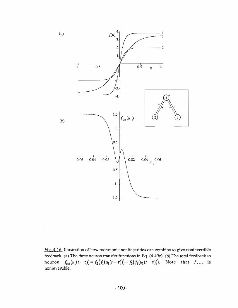
(a) 4. f(1/)
3.
2.
l.
-l. -D.5
-4.
1.5
(b)
-D.06 -0.04
-1.5
l 3
2
0.5 II l.
A
0.04 0.06 II l
Fi g:. 4.16 Illustration of how monotonic nonlinearities can combine to give noninvertibie feedback. (a) The three neuron transfer functions in Eq. (4.49c). (b) The total feedback to
neuron ftot(ul(t-"l"))=h(.fi(ul(t-"l")))-h(.fi(uj(t-"l"))). Note that fIOl is noninvertible.
- 100 -
4.7. DISCUSSION AND REVIEW OF RESULTS
This chapter is quite long and contains a number of new results. This final section is
included IO provide a summary of its contents.
We have considered the stability of analog neural networks with delayed response.
The aim has been to extend the stability condition: "symmetric connection implies no
oscillation" - which is valid when the neuron S have instantaneous response - to a more
realistic modelof neural networks where time delay is included. We find that
symmetrically connected networks can show sustained oscillation when the neurons have
delayed output, but only when the ratio of delay to relaxation time exceeds a critical
value.
At low neuron gain, linear stability analysis about the origin suggests that for
1: < -n/(2f3Åmin) asymmetric network will not oscillate. In this inequality, 1: is the
neuron delay in units of the network relaxation time, f3 is the gain (maximum slope) of
the neuron transfer function at the origin and Åmin is the minimum eigenvalue of the
connection matrix Tij as defined in Eq. (4.3).
The stability criterion based on linear stability analysis is valid at all values of gain but
becomes overly conservative in the large-gain limit. We find experimentally and
numerically that symmetric networks with extremal eigenvalues satisfying
IÅmaxlÅminl> I do not oscillate as long as the delay is comparable to or less than the
network relaxation time. In contrast, symmetric networks satisfying IÅmaxiÅ.-minl < I do
show coexisting fixed point and oscillatory attractors at large gain. There exists a critical
delay Teri! in the large-gain limit below which oscillatory attractors vanish and only fixed
points attractors are observed. For symmetric networks in which the oscillatory mode
present for the smallest delay is coherent (as defined in § 4.4.1), sustained oscillation
vanishes for" < "eri! = -ln(1 + Åma.,JÅmin)' This result is independent of gain and
- 101 -

is useful as f3 ~ ~, unlike the linear stability result (Eq. (4.17)).
The stability criteria have been tested numericaIly and in the electronic neural network
described in Ch. 3. Agreement between theory, experiment and numerics is very good.
Some results for particular network topologies:
(a) The all-inhibitory nel\~'ork is the most oscillation-prene eonfiguration of the delay
network. For this configuration, the critical delay in the large-gain limit is given by
"eri! = In«N-2)/(N-I)) - l/N, where N is the size of the network. Diluting the a11-
inhibitory network by randomly - but symmetrically - sening a smalt fraction d« l of
the intereonneetions (Tij and Tji) to zero will increase the critical delay by a factor of
(4dN) 1/2.
(b) Rings of symmetrically connected delay neurons will oscillate only when the ring
is frustrated (Sgn(Il ring Tij) = -1) and when there is an odd numbeT of neurons in the
nng.
(c) The critical delay for large two-dimensional networks with nearest-neighbor
lateral inhibition ean be either finite OT infinite, depending on the type of lanice. For zero
self-conneetion, Tcril ~ ~ as N ~ ~ for a square lattice, and Tcril ~ ln(2) = 0.693. .. as
N ~ ~ for a triangular lanice.
(d) The Hebb rule, Eq. (5.13), satisfies IÅmaxlÅminl > l and, as expected, does not
show sustained oscillation numerically OT in the electronic network for any observed
(finite) delay. Clipping algorithms, which limit the interconnections to a few strengths,
can introduce large negative connection eigenvalues and produee sustained oscillation in
networks with delay smaller than the network relaxation time.
Finally , we have discussed chaotic dynamics in asymmetric neural netwoTks. An
example of a chaotic three-neuron network with a single time delay was presenled. A
conneetion was made between asyrnrnetric nelworks of monotonie analog neurons and a
well-studied ehaotie system thaI has noninvertibie or "mixed" delayed feedback.
- 102-

Chapter 5
TRE ANALOG ITERATED-MAP NEURAL NETWORK
5.1. INTRODUCTION
In this chapter, we analyze in detail the dynarnics of an analog neural network with
discrete-tirne parallel dynamics. Because the network's dynamical equatians form a set
of caupled iterated maps, we will refer to the system as an iterated-map neural network.
The main purpose of this chapter is to show that the notorious problem of sustained
oscillations associated with parallel dynamies can be eliminated by using analog neurons.
Specifically, we present a global stability criterion that places an upper limit on the gain
(maximum slape) af the neuron transfer function. When satisfied, this criterion
guarantees that a syrnrnetrically connected iterated-map network will always converge to a
fixed point [Marcus and Westervelt, 1989c]. As an application, we treat the problem of
associative memory, and present novel phase diagrams for analog associative memories
based on the Hebb rule and the pseudo-inverse rule [Marcus et al., 1990J. These results
show that analog associative memaries ean be updated in parallel over a braad range of
neuron gains and storage ratios while maintaining good recaU and guaranleed
. convergence IO a jixed point. This feature distinguishes analog networks from the
standard Ising-spin netwarks (with ar withoU! temperature) which, in general, must be
updated sequentially to prevent oscillation.
We will also discuss a secand irnponant advantage of analog associative memories,
which is that lowering the neuron gain can greatl y increase the chances that an initial state
- 103-

far from all memories will correctly flow to a recall state without gelting trapped in a
spurious attractor.
The subsections of Ch. 5 are organized as follows. In § 5.2 we define the iterated
map neural network and prove !hat for a broad c1ass of transfer functions and symmetric
connections, the only attractors are period-2 limit cycles and fixed points. In § 5.3, we
then show that all limit cycles can be eliminated by lowering the neuron gain belowa
critical value. In § 5.4, we investigate analog associative memories based on the Hebb
rule [Hebb, 1949; HopfieId, 1982] and the pseudo-inverse rule [Personnaz et al.,1985;
Kanter and Sompolinsky, 1987), and present phase diagrams in the parameter space of
neuron gain f3 and memory storage ratio a. In § 5.5, numerical results for the
associative memory networks are presented. These results agree well with the analytical
results of § 5.4. The numerical results in § 5.5 also show that the probability of retrieval
is increased at low analog gain, suggesting the use of analog annealing to enhance recall.
Applications of these results and conclusions are presented in § 5.6. Some lengthy - but
important! - details are presented in two appendices: In appendix 5A, the storage capacity
of the Hebb rule for the analog iterated-map network is deri ved. This analysis
generalizes the cavity method approach of Domany et al. [1989J. In appendix 5B,
storage and recall properties of the pseudo-inverse rule are deri ved.
5_2. ITERATED·MAP NETWORK DYNAMICS
The dynamicaI system investigated in this chapter is an iterated-map neural network in
which all neuron s have continuous input-output transfer functions and updating is done
in parallel [Marcus and Westervelt, 1989c]. The network is defined by the set of coupled
nonlinear maps,
- 104-

(5.1)
where the real variables Xj(l) describe the state of the system at time l. Time. in its
present usage. is a diserete index: t = 0.1.2 •...• and ean equivalently be thought of as a
layer index in a feed-forward network with identieal eoupling between eaeh layer (cf.
[Meir and Domany. 1987; 1988]). The intereonneetion matrix Tij is assumed real and
symmelric. We also assume that the neuron transfer functions Fj are all single-valued
and monotonic (without loss of generality. we take all F j to be monotonicaIly
increasing) and may be different for eaeh i. Notice that the functions F j ean be
coneave-up or eoneave-down at any finite argument and do not need to saturate to a finite
value. However. to insure that the Liapunov functions presented below and in § 5.3 are
bounded below. we require that all F i increase in magnitude slower than linear for large
negative and positive argument. An example of a neuron transfer funetion that satisfies
these conditions is illustrated in Fig. 5.1 (a). The maximum slope of each Fj is defined
as the gain øj for that neuron. as shown in Fig. 5.1(a).
There is a completely equivalent form of Eq. (5.1) that has the neuron transfer
functions inside of the sum:
Uj(t+ l}/Rj = ~);jfj(Uj(t)) +l j (5.2) J
Equation (5.2) describes the evolution of the neuron inputs u/t) rather than the outputs
x/t). and is related to (5.1) by the change of variables:
(5.3)
- 105-

Ca) F; (x)
x
(b) F(x)
x
. Fig. 5.1. (a) An example of a non linear neuron transfer function which meets the conditions for the dynamic properties given in § 5.2 and § 5.3. Those conditions are: Each function must be single valued and monotonic, and must grow in magnitude slower than linear in the limit of large positive or negative argument. The maximum slope f3i that appears in the stability criterion (5.11) is also indicated. (b) An example of a nonlinear function F (idemical for all i) which meets the less general conditions assumed for the associative memory phase diagrams, Figs. 5.3 and 5.4. These conditions are given at the beginning of § 5.4.
- 106-

The continuous-time version ofEq. (5.1), given by
(5.4)
has the same fixed points as the iterated-map system (5.1), but not the same stability
properties: For Tij symmetric and all F j monotonic, Eq. (5.4) will always converge to a
fixed point, regardless of neuron gain. Finally, we note that the cominuous-time system
(5.4) is equivalent to the elecll'onic circuit equations used in chapters 3 and 4,
Cj dU j(r')/dt'= - uJt')/ Rj + I,T;}iAUj (c')) + lj j
(5.5)
when the time constants RICj are equal for all i. Equation (5.4) ean be transformed imo
(5.5) by the change of variables (5.3), plus the rescaling of time, r' '" (RjCj ) t.
We will now prove that all attractars of the iterated-map network (5.1) - or,
equivalently, all attractors of (5.2) - are either fixed points ar period-2 limit cycles
[Marcus and Westervelt, 1989c]. The proof consisrs of showing that a function E(t),
defined as
i,j
where
+ I, [Gj(Xj(t))+Gj(xj(t-I))] , j
- 107-
(5.6a)
(S.6b)
is a Liapunov function for the iterated-map network, Eq. (5.1), and that the minima of
E(t) are at either fixed points er period-2limit cycles ofEq. (5.1).
The change in E(I) between times I and Hl, defined as L1E(t) '" E(I+l) - E(t),
can be found from (5.6a) and (5.1) and the symmetry Tij= Tji, and is given by
where L12Xj(l) ",xj(l+l)-xj(l-l) is the change in xi(r) over rwo time steps. For
Gi(x) cencave up at all values of its argument x, we can write the folIowing inequality
(see Fig. 5.2):
(5.8)
where G[(Xj(l+l)) is the derivative of Gi(x) at the point x =xi(Hl). The case ef
equality in (5.8) only occurs when L1 2Xj(t) = O. The requirement that Gi(x) be concave
up is not very restrictive: it is satisfied as long as Fi is a single-valued, invertible, and
increasing function. Insening the inequality (5.8) into (5.7) gives
The difference in the square braeket equaIs zero by Eq. (5.6b) giving the result:
M(I) S;O
L1E(t) =0 => L12xJt)=0
- 108-
(5 .9)
(5. lOa)
(5.10a)
Thus E(r) is a Liapunov function for the iterated-map network (5.1) and all attraclOrs of
(5.1) - where .1E(t)=O - satisfy .12Xi(t) = O, orxj(t+l) =xj(r-l) for all i.
Therefore all attractors of (5.1) are either fixed points or period-2limit cycles.
5.3. A GLOBAL STABILITY CRITERION
In this section we show that all period-2limit cycles of the iterated-map network (5.1)
can be eliminated, leaving onJy fixed points, by lowering the neuron gains f3j to satisfy
the stability criterion:
1 > -Amin for all j ,
f3i (5.11)
where {3j ( > O) is the maximum slope of F i and Åmin is the minimum eigenvalue of the
connection matrix Tij [Marcus and Westervelt, 1989c). This criterion applies for any
distribution of the (real) eigenvalues of Tjj' When T jj has negative eigenvalues,
Ålnin( 'lij) refers to the most negative eigenvalue. Assumptions made abeut the network
in proving this result are the same as aiready used in § 5.2. As areminder: The
eonneetion matrix Tij is symmetrie and the neuron transfer funetions F i are single
valued, monotonie and inerease in magni tude slower than linear at large positive or
negative argument
The stability criterion (5.11) is derived by showing thaI the funetion L(t), dermed as
(5.12)
with Gj given by Eq. (S.6b), is a Liapunov funetion of (5.1) when the srabiliry criterion
- 109-

is obeyed, and that the minima of L (t) are at fixed points of (5.1).
From (5.1), (5.12) and the symmetry Tjj = Tjj, the ehange in L(r) between times
t and t+1, defined as LIL(t) '" L(t+1) - LU), ean be written
LIL(t) = -{I,1;j .1x;(t) .1Xj(t) - L fj-l(Xi(t+l)).1Xi(t) i,j
+ I.[ Gi(Xi(t + l)) -Gi(Xi(t))] , (5 . 13)
where .1Xj(t) '" Xj(t+1) - Xj(t). Note that .1x;(t) is the ehange in Xj(t) in one
time step.
We now eonstruct an inequality similar to (5.8), but including a quadratic term along
with the linear term. Choosing the coefficient of the quadratic term to be the minimum
curvature of G j(xj),
min(d2GJdx/)=f3i- l , x,
yields the folIowing inequality, as illustrated in Fig. 5.2:
Equations (5.13) and (5.15), and the equality G'j(Xj) = F(I(Xi) from (5.6b) yield
LIL(t) $; - t L [:r;j + '\f3i- I ].1xi (t).1xj (t) i,j
(5.14)
(5.16)
where Ojj = 1 for i = j and Ojj = O for i ~ j. As long as the matrix (T + B-I) - which
appears in componem form in the square braekets ofEq. (5.16) - is positive definite, then
the right side of (5.16) is negative, and, in that case, we can immediately write
- 110-

Fi (z)
, ,
t t A B
J
Fig. 5.2. Graphical representation of inequalities (5.8) and (5.15) for a typical sigmoid nonlinearity Fi(z) with maximum slope f3i (inset). The concave-up function G i (xi)
is defined in Eq. (5.6b). A line and a parabola with second derivative f3(1 ~ minx [d2G(x)/dx2j are tangent to the curve Gi (Xi) at the point [xi(t+l), Gi(xj(t+I»].
Eq. (5.15) is represented by the inequality C S; B; Equation (5.8) is represented by the inequality C S; A where the case of equality, C ~ A, implies L12xi (t) = O .
- 111 -
L1L(t) $ o L1L(t) =0 => LlXi(t)=O .
(5.17a)
(5.17b)
Thus, as Ion g as (T + B-l) is a positive definite matrix, L(t) is a Liapunov function for
the iterated-map system (5.1). At the minima of L(t) the condition Llxi(t) = O holds
for all i, thus all attractors are fixed points. A sufficient condition for (T + B-l) to be
positive definite is f3(1 > -Amin for all i. This condition is therefore sufficient to
guarantee that L(t) is a Liapunov function and that all minima of (5.1) are fixed points,
which gives the stability criterion (S.II).
5.4. ANALOG ASSOCIA TlVE MEMORY
We now apply the iterated-map neural network to the problem of associative memory
[Marcus et al., 1990]. In this section we assume a less general form for the network,
one in which Ii = O for all i and the nonlinear functions F i are single-valued, odd
functions and are the same for all i. We also assume the function F (now dropping the
index i) has its maximum slope at zero input, F'(O) = f3 , and that the slope of F is a
non-increasing function of the magnitude of the argument. As before, the maximum
slope f3 will be referred to as the gain of the neurons. Possibie fonns for F include,
but are not limited to, tanh-like functions including the transfer function for the e!ecrronic
network, Eq. (3.3 ). As in § 5.3, we do not require that F saturate at large argument
though it must increase in magnitude slower than linear at large positive or negative
argument. We nonnalize the amplitude of F so that the accessibie state space ("the
hypercube") is of length 0(1) on a side; that is, nonzero solutions of m' = F(m') are
typically 0(1). Fig. S.I(b) shows a function which meets the conditions assumed in this
section. Under these assumptions, the associative memory network is given by the set of
- 112-

coupled maps
i = l, ... ,N. (5.18)
We will consider connection matrices Ti} for two leaming rules, the Hebb rule and
the pseudo-inverse rule, storing random unbiased memory patterns, ~i/L = ±l. For the
Hebb rule,
where aN is the number of stored memory panerns. For the pseudo-inverse rule
aN r..=..!.." J;I'(C-!) J;V ,
IJ N L... '>, BV"'J 1'. v=! ~
where ~ l is the inverse of the correlation matrix,
N _ I " ):I'J;V
CI'V - N L... '>i '>i i=l
(5.19)
(S.20a)
(S.20b)
Notice that we are considering the modified pseudo-inverse rule with TU = ° studied by
. Kanter and Sompolinsky [1987). These authors showed that this modification increases
the basins of attraction for the memories without sacrificing error-free recaU. The
analysis in the folIowing two subsections assumes f3 > 0, 0< a < 1 and
N » l.
- 113-

5.4.1. Hebb rule
A phase diagram for the Hebb role, showing four distinct regions in the parameter
space of analog gain {3 and the storage ratio a, is presented in Fig. 5.3. The four
regions are characterized as follows: In the region marked 'origin' a fixed point at the
origin, Xi = ° for all i, is the global attractor. In the region marked 'spin glass' the
origin is no longer an attractor, but neither are the memory recall states. In this region,
the network converges to a fixed point with small [O(N-l!2)] overlap with all memories.
In the region marked 'recal!', fixed points having large overlaps with memory pauems
exist and have large basins of attraction. In the 'recal!' region the iterated-map network
operates well as an associative memory. The boundary separating 'recal!' from 'spin
glass' is shown in Fig. 5.3 for the particular choice F(z) = tanlz({3z). With thi s
choice of nonlinearity, this boundary agrees with the ferromagnetic transition curve found
by Amit et al. [1985b; 1987] for the Ising-model associative memory at finite
temperature. The present analysis leading to this curve, however, is not restricted to case
F(z) = tanlz({3z). Details are given in appendix SA. In the region marked
'oscillation' the stability criterion (5.11) is no longer obeyed and convergence to a fixed
point is not guaranteed. Numerically, we find that limit cycles are quite abundant in this
region, especial!y for larger values of {3 and a (see § 5.5).
The stability of the origin can be determined by linearizing Eq. (5.18) about the point
Xi = 0, which gives N decoupled linear iterated maps: qJi(t+I) = {3AjfPi(t) for
evolution along the itll eigenvector of the matrix Tij,with associated eigenvalue Ai. (cf.
Eq. (4.S), the corresponding equation for the delay-differential system). For 1{3\ I < I
for all j, the origin is stable, and because of the form of F, il is also the global attraclor
of Eq. (5.18). (The proof of this is based on a contraction mapping theorem. See:
Ortega and Rheinboldl [1970], Thm 12.1.2].) Notice that when the eigenvalue spectrum
- 114-

0.15 spin glass
a oscillation 0.10 ongm
0.05 recall
o .00 '-----~~~~--'--"'<'-----~~~~'-'--'---~~~~ .1 1 10 100
f3
Fil:. 5.3. Phase diagram for the Hebb rule associative memory with neuron transfer function F(z) = tanh(f3z). The parameter f3 is the neuron gain, and a is the number of stored patterns divided by the number of neurons N. All borders separating the regions are based on analysis at large N, as described in the text
- 115 -

is "skewed negative" (O < Ama .. < -Amin)' the stability eondition for the origin IS
identieal to the global stability criterion (S. 11).
The minimum and maximum eigenvalues for the Hebb matrix (S.19) with a < 1 in
the large-N limit are
Amax = 1+ 2..J(i ,
[N(l- a) - fold degenerate]
[edge of continuous distribution]
(5.21a)
(S.21 b)
[Geman, 1980; Silverstein, 1985; Crisanti and Sompolinsky, 1987], thus for a < 1 the
boundary where the origin loses stability is given by the condition f3 = 1/(1 + 2..J(i).
From the value of Amin in (S.21 a) we ean also identify the border of the oscillatory
region as f3 = Ila. Crossing the 'origin'-'spin glass' line corresponds to a forward
pitchfork bifurcation of the origin, analogous to aseeond order transition in
thermodynamies. Note that this transition oceurs along a different eurve from the
corresponding paramagnet-spin glass transition in the Ising model associative memory
[Amit et al., 1985b; 1987].
Crossing the border from the 'recaU' region into the 'spin glass' region marks the
disappearanee of a fixed point having a large overlap with a single memory. As in the
case of the Ising model network, this transition is due to the random overlaps of the state
of the network with pattems other than the one being reealled. These overlaps generate
an effective noise term whieh destabilizes the fixed point near the recalled pattern.
Because our system has no reaction fieid, the analysis is somewhat simpier than either the
replica [Amit et al., 1985b; 1987] or eavity [Mezard et al., 1987; Domany et al., 1988]
approaches used to anal yze the thermodynarnic Ising model network. In appendix 5A we
derive a set of four self-eonsistent equations that determine the border between the 'recal!'
and 'spin glass' regions assuming random, unbiased memory patterns:
- 116-

(5.22a)
(5.22b)
(5.22e)
..jaq (Y=--
l-C (5.22d)
where F'(z);: dF(z)jdz. The quantity ml in Eq. (5.22a) is the overlap of the network
state vector with a single memory pattem, arbilrarily chosen to be pattem l. In the recaU
state, these equations have a self-consistent solution with ml - l. For the panicular
choice F(z) = tanhC{3z), the quantities C and q obey the usual Fischer relation
C=j3(I-q) [Fiseher, 1976].
5.4.2. Pseudo-inverse rule
The pseudo-inverse learning rule, Eq. (5.20), offers several advantages over the
Hebb rule, chiefly a greater storage capacity, error-free recaU states and the ability to store
correlated pattems [Personnaz et al.,1985; Kanter and Sompolinsky. 1987]. Its primary
disadvantage is that it is nonlocal, meaning that a given element of the connection matrix,
T ij' cannot be determined from the ith and jth elements of the memory pattems, but
depends on all components of all memories. However, iterative learning algorithms have
been presented which are local and which converge IO the pseudo-inverse rule [Diederich
and Opper, 1987].
A phase diagram for the pseudo-inverse rule showing three distinct regions
depending on analog gain {3 and storage ratio a is shown in Fig. 5.4. This phase
diagram differs from that of the Hebb rule in three distinctive ways: First, there is no
- 117-

0.6
a 0.4 oscillation
ongtn
0.2 recall
0.0 L.~~~~_~~~.........L_"""""'::::::::::;::;::::::d .1 1 10 100
f3
Fig. 5.4. Phase diagram for the pseudo-inverse rule (diagonal elements = O) with sigmoidal neuron transfer function as described at the beginning of § 5.4. The parameter f3 is the neuron gain, and a is the number of stored patterns divided by the number of neuron s N. All borders separating the regions are based on analysis at large N, as described in the text. Note that the pseudo-inverse rule does not possess a spin glass phase for a < 1.
- 118-

'spin glass' phase. This does not imply that the pseudo-inverse mIe does not pos ses s
spurious attractors; just as for the Hebb rule, there are many spurious fixed point
attractors within Ihe recall and oscillalory regions which have small overlap with all
memories. Unlike the Hebb rule, however, there is no region of the pseudo-inverse
phase diagram where only spurious fixed-point attractors are found. The second
di fference is that Ihe recall region is much larger, extending to a = O.S for {J = 2.
Above this point, and for higher gain, recaU states still exist, but convergence IO a flxed
point is not guaranteed. The third distinctive feature is the adjacency of the 'origin' and
'oscillation' regions at larger values of a. Crossing the border between these two
regions, say by increasing {J, constitUles a multiple flip bifurcation [Guckenheimer and
Holmes, 1983] in which N(l-a) eigendirections about the origin simultaneously lose
stabiliry giving rise to period-2 limit cyc\es in the subspace orthogonal to all memories.
As in the Hebb rule phase diagram, the region marked 'origin' for the pseudo-inverse
phase diagram satisfies i{JÅi I < l for all i, where Åi are the N eigenvalues of the
pseudo-inverse matrix (S.20). For TU = O, the extremal eigenvalues in the limit of large
N are given by
A.min = -a,
Åmax=l-a
[N(l- a)- fold degenerate]
[Na - fold degenerate]
(S.23a)
(S.23b)
[Kanter and Somplinsky, 1987]. Belowa = O.S the origin loses stability at gain
{J = l/(l-a). This condition defines the border between the regions marked 'origin'
and 'recaU.' In appendix SB we show that stable recall states appear as soon as this
bifurcation occurs. From the stability criterion (5.11) and Eq. (5.23a), convergence to a
fixed point is not guaranteed for {J > l/a, which defines the region marked
'oscillation' in Fig. S.4.
Adding a positive diagonal element TU = r > O to the connection matrix shifts the
- 119-

1.0
0.8
0.6
a
0.4
y=0.3
0.2
y=O y=O.1
o 0.1 1 10 100
f3
Fig. 5.5. The recaU region for the pseudo-inverse rule for various values of diagonal element r Note that the maximum capacity in the recaU region is for analog gain f3 = 2, regardless of y. Although the recaU region is expanded for positive diagonal element, too large a diagonal will greatly reduce the basins of attraction for the recaU states, as discussed by Kanter and Sompolinsky [1987].
- 120-

eigenvalues to Åmin = -a + y and Åmax = 1- a + y and increases the maximum
storage capacity in the recaU region to amax = 1/2 + y. l The recaU region for several
values of positive self-coupling are shown in Fig. 5.5. Note that the maximum always
occurs at {J = 2. Recently, Krauth et al. [1988] have demonstrated that using a small
positive diagonal element with the pseudo-inverse rule in an Ising network (at zero
temperature) increases the radius of attraction for the recall states2 For example, they
find numericaUy that for a = 0.5, using a diagonal term of -0.075 instead of zero
increases the basins of attraction by about 50%. Too large of a diagonal term, however,
greatly reduces the basins of attraction for the recall states [Kamer and Sompolinsky,
1987; Krauth et al., 1988].
5.5. NUMERICAL RESULTS
5.5.1. Numerical verification or the phase diagrams
In this section, phase diagrams for the Hebb rule and pseudo-inverse rule are
invesligated numerically for networks of size N = 100 wilh F(z) = tanh({Jz) and
random, unbiased memory patterns. The data in Figs. 5.6 and 5.7 show, as a funelion
of analog gain /3, lhe fraction or randomly ehosen initial states which converged to a
particular type of attractor - either the origin, a memory pattern (or its inverse), a spurious
fixed point, or a period-2 limit cyele. These attractor types are the only possibilities.
Each panel in these figures is for a fixed value of a, so eaeh represents a horizontal slice
through the phase diagrams for the Hebb rule (Fig. 5.3) or the pseudo-inverse rule
t This definition of y dirrers from the one used in chaptcr 4: Here, the mauix elements T jj are equal to r. In chapler 4, the value y is the diagonal matrix element before normalization. See, for example. Eq. (4.18).
2 Krauth er al. (1988) use yet another definition of r. For them. Tjj = xl-a) for large N.
- 121 -

(Fig. 5.4).
The data in each panel were generated as follows: For each of 38 values of {3,
ranging from {3 - 0.3 to {3 - 90, twenty Tij matrices were generated using random,
unbiased panems, er = ± 1 . For each matrix, 50 initial states located at random comers
of the state space (xj(O) = ±1, i = 1, ... ,100) were chosen and the attractor for each was
found by iterating the map, Eq. (5.18). The condition for convergence was
Ilx(t) - x(t - 2)11 < 10-6, where distances are defined by IIzll E (l/2N)"L:;!zil. Though
the initial states were located at the comers of the hypercubic state space, all attractors
were real-valued N-vectors located away from the comers of the stale space. Plotted in
each panel are the fractions of the 20xSO = 1000 runs for each value of f3 which
converged to each of the four attractor types. A fixed point x * was counted as a recall
state if, for any 11,l!sgn(x *) ± ~JlII < 0.05; similar criteria were used to recognize the
other attractor types.
Along the top of each panel in Figs. 5.6 and 5.7 is a strip marked 'orig.' , 'recall',
etc. These strips show the regions of the theoreticaI ph ase diagram (from Figs. 5.3 and
5.4) for the particular value of ex in that panel. The appearance of the various altractor
types corresponds very closely to the theoretical regions in these slices, giving strong
numerical support to the phase diagrams. Furthermore, the data indicate that the basins
of attraction for limit cycIes in the 'oscillation' region do occupy a significant part of state
space as soon as the stabil it y criterion is violated. That is, the 'oscillation' region is more
than just the region where convergence to a fixed point is not guaranteed by the stabil it y
critenon, it is in faet the region where oscillatory modes are quite abundant.
- 122-
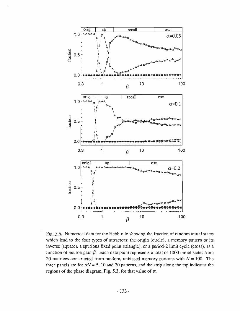
"
ong. I sg I recall I ose. 1.0 ctG&&G /\ ....... a=O.OS
~
! I \
\f \ . .., ."...,('-c...,
,I \ I
0.0
0.3
i, \ I, j \ ".trl{'~"'''''".-I ~ \ ~
" .... ~ ;. ., .... -. &.
1 f3
10 100
orig. I sg I rccall I osc. 1.0 G-G &G.
" /I'rl!r-r\ a=O.1 ' i ~ .... ! , 4\ ! J \
\1 A.. tr6.. A _A lr-tr"--............ r- I A-
l
/: -.,. ~,
l!
. 9 ~ 0.5 <l::
§
0.0
0.3
orig. I
,! ,! ,~
J. \.
l
SiL
'~~ G&GO
f3 10 100
I osc. 1.0 o G Q. A~b-6-b-Irlrl>-Irlrl>-~...... a=O 2
Q I ~~~ . 'f -..."..... , l>"<> , f -.,
" .~ 0.5 ;j
I i,
..= " ,., , ,
;'~., ~ :~;:::: ..•..•.•.•.... ~iiii~O;;;:~;~~@~ge 0.0
0.3 1 f3
10 100
Fig. 5.6. Numerical data for the Hebb rule showing the fraetion of random initial states whieh lead to the four types of attractors: the origin (circJe), a memory pattem or its inverse (square), a spurious fixed point (triangle), or a period-2 limit cyc1e (eross), as a function of neuron gain f3. Each data point represents a total of 1000 initial states from 20 matrices constructed from random, unbiased memory pattems with N = 100. The three panels are for aN = 5, 10 and 20 pattems, and the strip along the top indicates the regions of the phase diagram, Fig. 5.3, for that value of a.
- 123 -

orig. 1.0 :..o.-~&&~e-e- 9
.9 l.l 0.5
.t:
" o ·0 ~
.t:
0.0
0.3
1.0
0.5
0.0
0.3
, ; , ,
1
ori
1
ori~.
; ~ · 1 !I
J J . ,
I 1.0 OGe e-(}e-e- G&~
§ '.0 0.5 ~
.t:
0.0
0.3 1
, , , ,
, , , , ;
recaU 1 osc.
-........ a=O.l
C" ....,.
/~-"",,",,"f>.t, Ir~
~~".4 ", o-eo-o
fJ 10 100
ose.
a=O.25
fJ 10 100
osc.
a=O.7
fJ 10 100
Fig. 5.7. Numerical data for the pseudo-inverse rule showing the fraction of random initial states which lead to the four types af attractors: the origin (circle), a memory
pattern ar its inverse (square), a spurious fixed point (triangle), or a period-2 limit cycle (cross) , as a function of neuron gain /3. Each data point represents a total of 1000 initial states from 20 matrices constructed from random, unbiased memory patterns with N =
100. The three panels are for aN = IO, 25 and 70 pattems, and the strip along the top indicates the regions af the phase diagram, Fig. 5.4, for that value af a.
- 124 -

5.5.2. Improved recaU at low gain: deterministic anneaIing
Figures 5.6 and 5.7 show that the probability of recall is greater at lower values of
analog gain within the 'recaU' region. This phenomenon suggests apotentially powerful
technique for annealing a deteTministic analog neural network to a good (low energy)
solution [Hopfield and Tank, 19851 . Annealing by varying the analog gain is not only
useful as a fast numerical technique. but can be easily implemented in analog elecrronics.
eliminating the need for electronic noise generators to perform stochastic annealing.
As with standard simulated annealing (Kirkpatrick et al. , 19831. convergence times
at reduced gain can be quite long. To speed convergence, the gain should follow an
annealing schedule. starting at the low-gain border of the 'recall' ph ase. and ending at the
high gain border. The phase diagrams. Figs. 5.3 and 5.4. can be used to find the range
of gains over which annealing should take place. Note that annealing range depends
strongly on the storage ratio a. The surprising fact that the performance of an
associative memory can be improved by using analog neurons will be considered in more
detail in Ch. 7.
5.6. DISCUSSION
In this chapter we studied the dynarnics and associative-recaU properties of an analog
network with parallel dynarnics. We found that using analog neurons has two important
benefits: First, analog networks can be updated in parallel with guaranteed convergence
to a fixed point as long as the stability criterion (5.11) is satisfied. For the associative
memories considered. the iterated-map network has rather large regions in the space of
neuron gain f3 and storage ratio a where recall states exist and the stability criterion is
satisfied. The second benefit, seen numerically in Figs. 5.6 and 5.7. is that using a
- 125-

reduced neuron gain improved the chances that a random initial state would make it to a
memory state without getting caught in a spurious attractor.
The usefulness of analog dynamics goes beyond the stability and improved recaU
propenies studied here. By taking advantage of the generality of the stability results of
§ 5.3, one ean design stable networks of neurons having nonsigmoidal transfer
functions with computationally useful propenies. As an example, the stability results
apply to three-state (+1, O ,-1) neurons [Yedidia, 1989; Meunier, el a/., 1989]
generalized to a smooth 'staircase' analog transfer function. Networks of three-state
analog neuron S bear a strong resemblanee to the mean field spin-l Ising model at finite
temperature [Blume, 1966; Capel, 1966], with regions of parameter space where both the
origin and recaU states are locally stable. Such systems might be used to allow an '}
don't know' state of the network, sue h that initial states with insufficient overlap with
any pattem will converge to the origin. In a numerical investigation3
of networks made
of three-state analog neuron s, it was found that the attraetors inc!uded not only the recaU
states and the origin, but also new mixture states in which a pattern was partially recaUed,
with some neurons converging to the zero-output state.
Another generalization of the iterated-map associative memory is the de!iberate
inclusion of limit cycles as recall states. Several techniques for storing and recalling limit
eyc!es have been explored in continuous-time systems with delay [Grossberg, 1970;
Kleinfeld, 1986; Sompolinsky and Kanter 1986; Gutfreund and Mezard, 1988; Riedel,
et al., 1988; Herz, et al., 1988; KOhn, el al., 1989] and in discrete-time systems, both
for sequential [Buhmann and Schulten, 1987; Nishimori et al., 1990] and parallel
dynamics [Dehaene, er al., 1987; Guyon, el al., 1988]. Because these models use
asymmetrlc connections, !ittle is known analytically aboUl their stability or the types of
attractors they can produee. On the other hand, it is possibie to store 2-cycle attraetors in
3 This work was done by Fred Waugh.
- 126-

the iterated-map network using asymmetric connection matrix. This can be done most
easily with a generalized Hebb rule in which a weighted Hebb matrix for the osciliatory
directions 'v is subrracted from a Hebb matrix for the fIxed-point pattems ~11 :
1 [PIP po,,] N L~f'~f-ALsnr .
11=1 v=1
(S.24)
The weighting factor A can be uSed to cause fIxed point pattems and 2-cycle pallerns to
appear at different values of analog gain. A detailed analysis of such an analog network,
yielding for example the combined storage capacity of lirnit cycles as well as fIxed points,
remains an open problem.
APPENDIX 5A: STORAGE CAPACITY FOR THE HEBB RULE
In this appendix we fInd the border separating the 'spin glass' region from the 'recall'
region in the phase diagram for the Hebb rule, Fig. S.3. The derivation is a slight
generalization of a cavity method approach presented by Domany et al. [1989], but is
somewhat simpier because of the absence of the reaction fIeld [Marcus et al.,19901. The
form assumed for the nonlinear function F (taken to be identical for all i) is described at
the beginning of § S.4 . We also assume all memory patterns, ~iJ.l. = ±1, to be
uncorrelated, and we set li = O for all i. For the special choice F(z) = tanh(f3z), the
border we obtain is the same as that obtained for the Ising model network at temperature
1/f3 [Amit et al., 1985b; Arnit et al., 1987; Mezard et al., 1987; Domany et al.,
1989]. Throughout this appendix and appendix SB, sums over roman indices
(j, j, k, ... ) run from 1 to N; sums over greek indices (J.l., Y, p, ... ) run from 1
to aN.
A recaU state is characterized by the existence of a fIxed point of the iterated map,
- 127-

whieh satisfies
(SA.l)
and whieh has a large (0(1» overlap with a single memory pattern. where the overlaps
mil are defined
l ml' = - ~ J:!,xN .LJ '>. •
• (SA.2)
For the Hebb matrix. Eq. (S.19). the input hi to neuron i ean be wriuen in terms of the
mil as
It; = L T;jXj = L ~fml' (SA.3) j l'
whieh gives a set of aN fixed-point equations for the overlaps
ml' =2.L~fF(h;) , Jl=I, .... aN . N j
(SA.4)
For F odd and ~f = ±1, these equations ean be written
mIL = ~LF(~rh;)= ~LF(Hr)=(F(HIL)) • •
(SA.S)
where Hf '" ~r hj . Borrowing spin glass terminology, Hf will be referred to as a local
field for memory Jl. The braekets in (SA.S) denote an average over the index i:
- 128-

(z) = l/N Lli . In the large-N limit, this average ean be written as an integral over the
distribution of local fjelds P(HJl):
(5A.6)
We now seek a self-consistent expression for the distribution funetion P(H1) when
ml -l and mll - 0(N-112) for 11>1. The loeal fjeld for pattern 1,
Hl = glLgtmV , (5A.7) v
ean be split imo rwo parts,
H l l ):l"):v v i = m + '-;,i ~ ~i m . (5A.8)
v>l
For a - 0(1), the seeond term on the right side of (5A.8) aets as a noise term whieh we
take IO be gaussian distribuled wilh zero mean and varlanee (T2 given by
(5A.9)
To evaluate the sum of squares in (5A.9) we first write the overlaps m v wilh the
uneondensed pallems using (SA.3) and (5A.4):
(5A.IO)
Notiee that the right side of (5A.lO) is of the form L.AiBi' A sum of Ihis form with
- 129-

uncorrelared random variables Ai and Bi has an expected square of Lr4?B? In
(SA.IO) however, the two factors in the sum over i are correlated through the p =v
term in the argument of F , and this tenn must be treated separately before squaring.
Writing the correlated tenn separately,
(SA.!!)
and noting that the single tenn ( p = v) is small compared to the sum over all the rest
( p .. v), we expand F to fITst order in m v giving
(SA.12)
where F' is the derivative of the function F . The missing p = v term in the argument
of F' only affects the value of F' to order O(l/N) which we neglect by taking the
argument to be the whole hi' We now define the quantity C,
C'" (F'(h») = J.-L F'(h;) Ni
(SA.13)
and write (SA.12) as
(SA.14)
With the p = v term removed from the argument of F, the two factors in the sum over
i on the right side of (SA.14) are now uncorrelated and can be squared to yield an
- 130-

expected value of
(SA.IS)
where, again, the OO/N) error in the value of F2 from the p = v term is ignored.
Next, we defme the quantity q in analogy with the Edwards-Anderson order parameter,
(SA.16)
and write (SA.lS) as
(SA.17)
From (SA.9) and (SA.!7), the variance cl ofthe local field distribution is given in teons
of the quantities C and q by
(SA.18)
Beeause F' and F2 are both even funetions, we ean multiply their arguments by ±l
without ehanging their values. This allows us to write the averages in Eqs. (SA.13) and
(SA.16) in terms of Hl rather than hj, and finally as integrals over the distribution of
local fie1cls P(H1), given by the normalized gaussian distribution
1 l -H-m [( 11)2] p( H ) = ...fi7fa exp 2a2 . (SA.19)
- 131 -

where the variance a2 is given by (SA.18). Together with Eq. (SA.6), the self
consistent equations for quantities m I, C and q are given by the folIowing integrals:
ml = f dH1p(H1)P(HI)
c= f dHlp(H1)F'(HI)
q= JdH 1p(HI)p2(H 1)
(SA.20a)
(SA.20b)
(SA.2Oc)
Af ter a change of variables, y == (H l_ml l/a, Eqs. (SA.18) - (SA.20) yield the self
consistent set of equations (S.22a)-(S.22d) in § 5.4.1.
APPENDIX 58: RECALL STATES FOR THE PSEUDO-INVERSE RULE
In this appendix we show that for the pseudo-inverse learning rule, stable recall states
exist whenever a < I and {3 > l/(l-a) [Marcus et al.,1990). This implies that there
is no spin glass phase for the pseudo-inverse rule in the iterated-map network, in contrast
to the thermodynamic Ising-spin network with the same learning mie [Kanter and
Sompolinsky, 1987). The analysis below closely follows Kanter and Sompolinsky
[1987) .
As described in appendix SA, a recaU state is defined as a fixed point which has a
large overlap with a single pattern (again, taken IO be pattern l). For large N, Ihe single
large overlap ml can be written as an integral over the distribulion of local fieIds
(SB.1 )
- 132-
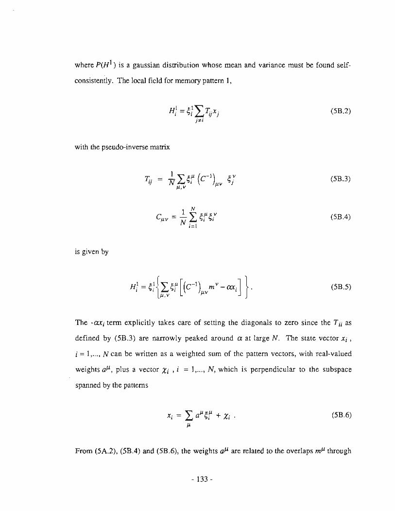
where P(H l) is a gaussian disoibution whose mean and variance must be found self-
consistently. The local field for memory pattern I,
wim the pseudo-inverse matrix
is given by
T = ~"J!p. (C-l) ;: v ij N L~. p.v ~ J
p., v
N _ I ,,;:p.;: v
Cp.v - N L ~i '>i i=1
(SB.2)
(SB.3)
(SB.4)
(SB. 5)
The -axi term explieitly takes care of setting the diagonals to zero sinee the Tii as
defined by (SB.3) are narrowly peaked around a at large N. The state veetor xi ,
i = I, ... , N ean be written as a weighted sum of the pattern veetors, with real-valued
weights all. plus a vector Xi ,i = I ..... N. whieh is perpendicular to the subspace
spanned by the patterns
Xi = IaP.~f + Xi' !'
(SB.6)
From (SA.2). (SB.4) and (SB .6). the weights all are related to the overlaps mJ.l through
- 133 -

the inverse correlation matrix
(SB.7)
Writing the local field Hl in terms of the aP-,
Hl = (1 - a )a1 + ~l (1- a)[ L ~i aJ.t] - aXi '
J.t > l
(SB.8)
reveals a similar structure to the Hebb mIe (compare (SB.8) to (SA.8)), with a 'signal'
term proportional to al and a 'noise' term due to the other patterns. The third term on
the right causes the state to relax towards the sllbspace spanned by the memories, and
does not add any destabilizing 'noise.' Comparing Eqs. (SB.8) and (SA.8) also reveals
why the pseudo-inverse mie allows perfect recall with an extensive nllmber of patterns
and the Hebb mie does not: for the pseudo-inverse mie, the variance of the gaussian
noise due to the other patterns is given by
(SB.9)
whereas for the Hebb mle, the variance is
(SB. IO)
When the state of the network is fIllly aligned with, say, pattern 1, then all aP-, J1 > I
vanish. On the other hand, the overlap s mJl, J.l > l do not vanish, even when the state
is perfectly a1i gned with a pattem, unless all memories are orthogonal. Therefore the
- 134-

'noise' term for the Hebb rule is in general always non-zero.
In a recaU state (for pattern 1), al = m l and a1l= O for J1 > 1, giving a delta
function distribution for the local fieids
(S8JI)
Inserting this distribution into (58.1) gives the self-consistent solution for the overlap
with pattem 1,
(58.12)
When the function F is tanh-like with maximum slope {3, there is a non-zero m l given
by (SB.12) whenever a < l and {3 > l/(l-a). The value of m l grows continuously
from zero at the transition. In analogy with thermodynamics, the appearance of recall
states is therefore a second order transition. As mentioned above, the behavior of the
analog network with the pseudo-inverse rule for the particular choice F(z) = ranh({3z)
is not the same as the corresponding Ising-spin network at finite temperature 1/{3: as
shown by Kanter and Sompolinsky [1987], the recall states for the Ising model appear at
avalue of {3 significantly above l/Cl-a) and the transition to the recaU state is first
order. These differences can be attributed to the absence of areaction field in our system.
- 135-

Chapter 6
TRE ANALOG MULTISTEP NETWORK
6.1. INTRODUCTION
In Ch. 5, we showed that analog neural networks offer several computational
advanrages over networks of binary neurons, including rhe property that convergenee ro a
fixed point under parallel dynamics ean be assured by a global stability eriterion for
networks with symmetric eonneetions. The purpose of this ehapter is to extend these
stability resuIts to networks with an updating rule based on multiple previous time steps,
and apply the new stability eriterion to the problem of associative memory.
The signifieam resuIt whieh emerges from this analysis is that the eriterion for
assuring eonvergence to a fixed point allows a larger neuron gain in proportion to the
number of time steps used in the updaring rule, while other properties, including the
storage eapaeity, are independent of the number of steps used. We emphasize that even
when many previous states are used in the updating rule, parallel is still parallel: Thinking
in terms of eleetronie hardware, one ean imagine using a tapped analog delay line I at
the input of eaeh neuron; upon eaeh time step, the local states at each neuron are
simultaneously advaneed one position in the delay line. In this scheme. previous time
steps are local and only need ro be evaluated once.
A further motivation for studying multiple-time-step networks is to provide a first
lDelay. linc dcvices are described in Mcad [1989). Commercial tapped delay lines are available, for example, from EG&G Relicon Corp. (see: EG&G Reticon Applicalion Note 105, A Tapped Analog Delay for Sampled Data Signal Processing.)
- 136-

step in the application of global stability analysis to networks that make explicit use of the
time domain as part of the computation, including recently proposed models for storing
and generating sequences of patterns [Grossberg, 1970; Kleinfeld, 1986; Somplinsky
and Kanter 1986; Dehaene, et al., 1987; Gutfreund and Mezard, 1988; Riedel , el al.,
1988; Herz, et al., 1988; Guyon, et al., 1988; Kiihn, el al., 1989]. Typically,
sequence-generating networks sample multiple previous states - for example by using
time delay - to determine their evolution. Numerical stucties [Riedel, et al. , 1988;
Babcock and Westervelt, 1986; Aihara et al., 1990] well as experiments using analog
circuits [Marcus and Westervelt, 1988] (see § 4.6) show that the neural networks with
time delay can be chaotic, and very few analyticaI results on their stability and
convergence are known [Marcus and Westervelt, 1989a] (see § 4.3 and § 4.4). The
analysis presented here is greatly facilitated by considering a relatively simple discrete-
time multi step system with symmetric connections. In this sense, our results apply to
sequence-generating networks when they are configured to retrieve fixed points only.
The dynamicaI system we will study is defined by a set of N coupled iterated rnaps
(6.1 a)
where zP) is the output of the ih neuron time-averaged over M previous time steps:
j = 1,,, .,N ; M E {1,2,3,,,.} (6.1 b)
This system will be referred to as a multislep neural network. Updating of the state
variables xi(t) as well as the z/t) is done in parallel (i.e. synchronously) and is fully
deterministic. We assume throughoul that the connection matrix T ij is symmelric. The
- 137-

(a)
(b) Fj( input)
x· l
input
Fig. 6.1. The analog multistep neuron. (a) Schematic representation of a multi step neuron with M = 3. Electronic implementation could use a tapped delay line as part of the input (or output) circuitry. (b) An example of a neuron transfer function F i (solid line) that satisfies the conditions required for the analysis: F i is monotonic, singlevalued, and increases in magnitude slower than linear at large argument. The maximum slope of Fi (dashed line) is defined as the neuron gain Pi'
- 138-

non linear neuron transfer funetions Fj must obey the same eonstraints as in Ch. 5: All
F j are monotonie (Without loss of generality, we ean choose all F j to be monotonically
increasing) and single-valued. Also, the F j may be locally concave up or concave
down, and do not need to saturate, but must eventua1ly increase in magnitude slower than
linear for large positive and negative argument. An example af a function F j that
sati sfies these conditions is shawn in Fig. 6.I(b). The maximum slope of each F i is
defined as the gain {3j for that neuron. ResuIts af § 6.2 and § 6.3 ean be applied to
networks af binary (Ising) neurons by letting all {3i ---> "".
Equation (6.1) with M = 1 is the standard analog iterated-map neural network
discussed in Ch. S [Marcus and Westervelt, 1989c]. The M = 2 case of (6.1 ) with all
F j = Sgn was investigated numerically by Kanter and Sompolinsky [1987] for an
associative memory neural network based on the pseudo-inverse learning rule. These
au thors found that the basins of attraction for the recall states are considerably larger for
M = 2 than for M = 1 (the basins for recall states under sequential updating are larger
than for either of these parallel schemes). Kanter and Sompolinsky [1987] offered the
folIowing explanation for this observation: First, the use of two previous states in the
updating rule adds an effective momenTUm to the dynamics, allowing the network to
"coast" over shallow local minima; Second, spurious oscil/atory attractors for this
network are 3-cycles, which, they argued, are rarer than the 2-cycles found in the
M = l network. Below, we will prove (for general F j ) the claim of Kanter and
Sompolinsky [1987] that the only attractors for M = 2 besides fixed points are period-3
limit cyc1es. On the other hand, numerical evidence for the M = 2 Ising spin glass
presented in Ch. 7 suggests that spurious 3~ycles may be quite abundant for multistep
networks.
The rest of the chapter is organized as follows. In § 6.2 we derive a global stability
criterion whieh guarantees that the multislep analog network will always converge to a
- 139-

fixed-point attractor as long as the maximum neuron gain f3 ;: maxi (f3i) does not exceed a
critical value which is proportional to the number of time steps M in the update rule and
inversely proportional to the minimum eigenvalue of the connection matrix. For the
particular case M = 2 we also prove that the only other possibIe attractors (i.e. when the
stability criterion is violated) besides fixed points are period-3 limit cyc1es. In § 6.3, we
apply these results to multistep associative memory networks and give a simple stability
criterion for the Hebb rule [Hebb, 1949, Hopfieid, 1982] and pseudo-inverse rule
[Personnaz, et al. , 1985; Kanter and Sompolinsky, 1987]. This criterion depends on
M, f3, the ratio a of stored memories to neurons and the self-coupling r In § 6.4,
we show that the convergence time of the multistep network inereases proportional to M,
but that in some instances, optimal choices for both f3 and M give faster convergence
with increasing M . Finally, conc1usions and open problems are discussed in § 6.5.
6.2. LIAPUNOV FUNCTIONS FOR MULTISTEP ANALOG NETWORKS
6.2.1. Global stability criterion for general M
In this section we prove that the analog multistep network, Eq. (6.1), will have only
fixed point attractors whenever
(6.2)
where f3;: maxj(f3i) > O is the maximum neuron gain, M E {1,2,3, ... } is the number of
time steps in the update rule and Åmin(1ij) is the minimum eigenvalue of the symmetric
connection matrix Tjt This criterion applies for any distribution of the (real) eigenvalues
of Tjt In particular, when Ti} has both negative and positive eigenvalues, Åmin(1ij)
- 140-

refers to the most negative eigenvalue. This result should be compared to the
corresponding result for the iterated-map network (the case M = l) presented in Ch. 5,
which is the stability criterion (5.11).
FolIowing a similar approach to Ch. 5, we consider the discrete-time evolution of the
real scalar function L(t) deflned
L(t) (6.3)
where
(6.4)
The requirement that F i change in magnitude slower than linear at large argument insures
that the function L(r) is bounded below.
The change in L(t) in one time step, deflned as L1L(t) '" L(t+ l) - L(r), is
L1L(t) = -~ ~ 7;;[ zj(r + l)zj(r + 1) - zj(r)zj(r)] I.)
1 + L M [Gj(xj(r + 1») - Gj(Xj(t - M + 1))]
I
1 -L-Ij[Xj(t+l)-Xj(t-M+l)] .
jM
. This ean be simplifled by defming the change in z/r):
1 .1z j (t) '" [zi(r + l) - zj(r)] = -[Xi (r + l) - Xj(t - M + l)]
M
and using the symmetry of Tij , giving
- 141 -
(6.5)
(6.6)

M(t) = -~ 2: Tij Lizj(t) Lizj (t) - L, Liz j (t)[L, JjjZj (t) + lj] t .) ')
1 + L, M[Gj(Xj(l+ J))-Gj(xj(t-M + 1))] .
I
(6.7)
Expanding the last term in (6.7) in a two-term Taylor series about the point Xj(t+ l) and
replaeing the eoeffieient of the quadratie term with the smallest value that it ean take,
which is
min(d2GJdx?) = f3j-l , Xi
(6.8)
gives the folIowing inequality [see Fig. 6.2):
where G;' is the derivative of Gj with respeet to Xj' From Eqs. (6.1a) and (6.4) , G;'
ean be wri tten
G/(Xj(t+l)) = F;- I(Xj(t+ 1)) = L,Tijz/t)+lj, j
leading to an inequality for Æ(t):
M(r) 1
< - -" y, . Liz-(r) Liz -(t) - 2~ I) I )
I.)
By defining a matrix Kij as
- 142-
(6.10)
(6.11)

F !
G · !
i t B A
~-.Æ
Fig. 6,2, Inequalities (6.9) and (6.20), illustrated for a particular transfer function F i (inset) and its corresponding Gi' defined by Eq. (6.4). The curve tangent to Gi on the right side is a parabola with second derivative {3i- 1 ,the line on the left is tangent to Gi' Equation (6.9) is the statement A ~ B. ; Eq. (6.20) is the statement C ~ D, and C = D
only when xj(r + l) = xi(r - 2).
- 143 -

K '" ~[T. + 8 .. Mn.-l] = ~ 'I 2 l' l' fJI 2
the inequality (6.11) can be rewritten in the simple form
LlL(t) ~ - L, Kij Llzj(t) Llzj(t) . i,j
, (6.12)
(6.13)
From (6.13) it is clear that if Kij is a positive definite matrix, !hen LlL(t) ~ O, and that
the case of equality (LlL(t) = O) only can occur when all Llz / t) = O. Writing the
ilifference of Eq. (6.1) at subsequent times as
L,'lij Llzj(t) = r;- l(xj(t+l)) - r;-l(X j( t») j
(6.14)
indicates that the condition Llz/t) = O for all i (and therefore the eondition M(t) = O)
further implies that Xj(t + l) = Xj(t) for all i ; that is, that the system must be at a fixed
point.
A sufficient condition for Kij to be positive definite is M fJi-) > -Amin(Ti) for all
i , where Amin(Ti) is the minimum eigenvalue of the matrix Ti} . (Thi s holds for any
value for Amin') In terms of the maximum neuron gain fJ '" maxj(fJ;), this sufficient
condition ean be stated
Kjj positive definite . (6.15)
- 144-

Equations (6.13) - (6.15) and the arguments in the preceding paragraphs can be
summarized as follows:
Srabjliry Criterion .
1 -> {3
=) (1) L(t) is a Liapunov function of system (6.1),
(2) All attractors of (6.1) are fixed points. (6.16)
As mentioned above, this criterion applies for any distribution of the (real) eigenvalues of
Til" When Tij has both negative and positive eigenvalues, Amin(T;j) refers to the most
negative eigenvalue. The stability criterion (6.16) is immediately satisfied if the
connection matrix Tij is itself positive definite (since M and {3 are both strictly
positive), although this is usually not the case in most currently-used network
applications (see § 6.3).
What can be said about the attractors of (6.1) when the stability criterion (6.16) is
not satisfied? For M = l, we showed in § 5.2 that the only new kind of attractor that
can appear when (6.16) is violated is a limit cyde of period 2. For M = 2, we will prove
in the following subsection that the only possibIe attractors besides fixed points are
period-3limit cycles. For M > 2 , we know of no results - analytical or numerical - that
limit the possibIe types of attractors of (6.1) when (6.16) is not satisfied. However, the
trend for M = 1,2 suggests that for general M, attractors of (6.1) (with symmetric Ti)
might be restricted to limit cycles with periods of (M+ I) and its divisors.
- 145 -

6.2.2. The case M = 2: Only fixed points and 3-cydes
The simplest multistep ex tension of the standard parallel update rule is the M = 2
case of (6.1). An Ising-model version of this network was stu<iied by Kanter and
Sompolinsky [1987] for the pseudo-inverse rule associative memory. These authors
found numericaIly that the M = 2 network has improved recall over the corresponding
standard (M = l) Ising-model network. As part of their explanation for the improved
performance, they also point out that the only non-fixed-point attractors for their network
were period-3 limit cycles.
In this subsection we prove a generalization of the statement of Kanter and
Sompolinsky [1987]: We show that all attractors of the multistep network (6.1) with
M = 2 are either fixed points or period-3 limit cycles for general nonlinearities Fi as
defined in § 6.1. Again, this result assumes a symmetric Ti)"
Consider the time evolution of the function E(I), defined
E(I) = - L. Ty [Zj(I)Zj(l-l)+~Xj(l-l)Xj(I-I)] I.,
2
+ ~ r r [Gj(xj(l-r))-ljXj(l-r)] i 1'=0
(6.17)
where the function Gi is given by Eq. (6.4). As with L(t), the requirement that all Pi
change in magni tude slower than linear at large argument insures that the function E(t)
is bounded below. The exact form of Eq. (6.17) was not deri ved, but was found via
guesswork and some intuition, though il bears an obvious resemblance to L(I) as well
as to other previously discovered Liapunov functions [Cohen and Grossberg, 1983;
HopfieId, 1984; Goles-Chacc el al., 1985; Golden, 1986]. The change in E(t) in one
time step, defined .1E(I):: E(I + l) - E(I), is
- 146-

LlE(t) = - I. T;j [zj(t+l)zj(t)-Zj(t)Zj(t-I)] i,j
+ ± ~ T;j [Xj(t)Xj(t)-xj(t-l)xj(t-I)] l.}
+ i I. [Gi(xi(t+1))-Gj(xj(t-2))-ljxj(c+l)+/jx;(C-2)]. (6.18) I
Expressing the first term an the right of Eq. (6.18) in terms of x/s and x/s (from
Eq. (6.1b)) and using the symmetry ofTjj , the change M(t) can be .... 'litten as
M(t) = - i ~ [Xj(t + l) - Xj(t - 2){ t-T;jZj(t) + li J 1
+ "2 I, [Gj(Xi(t+l))-Gj(Xj(t-2))]. I
(6.19)
We now expand G j to first order about the point Xj(t+l) and use the following
inequality [see Fig. 6.2]:
Equation (6.20) differs from the second-order expansion of G j used above (Eq. (6.9» in
that the only case af equality for Eq. (6.20) is when Xj(t + l) = Xj(t - 2). Combining
Eqs. (6.10), (6.19) and (6.20) yields
LlE(t) :s; -iI,[fi-1(Xj(t+1)) - Gj'(Xj(t+I))j{Xj(t+I)-(Xj(t-2))}. (6.21) I
From Eq. (6.10), the difference in square brackets equals zero, and therefore
- 147 -

.1E(t) s; o; .1E(t)=O ~ xj(t+1)-xJt-2)=Oforalli.
(6.22a)
(6.22b)
Thus, E(t) is a Liapunov function for the system (6.1) with M = 2, and all attractors
(the minima of E(t» satisfy the condition Xj(t + l) = Xj(t - 2) for all i. That is, all
attractors are either period-1 (flxed points) or period-31imit cycles.
6.3 MULTISTEP ASSOCIATIVE MEMORIES
To illustrate some of the beneflts of using a multistep update rule, we now consider
associative memory networks based on the two learning algorithms studied in Ch. 5: the
Hebb ru1e and the pseudo-inverse rule. The connection matrices Tij to be insened imo
the multistep network (6.1) in order to store a set of p flxed-point memory pattems ~,jl
(~f= ±1; i = 1, ... , N; 11= 1, ... , p) are specified by the following rules:
HebbRule:
Ii} =
Pseudo-inverse Rute:
1 p
N L ~/' ~/ (i ... j)
r
r
}L=\
(i = jl
1 N C =_"J;)lJ;v
}Lv N ~." ." ;=1
- 148 -
(6.23)
(i ... jl (6.24a)
(i = jl
(6.24b)

We take the self-coupling term y to have an adjustable value in both learning mies. The
influence of self-coupling y on the recaU performance [Kanter and Somplinsky, 1987;
Krauth et al., 1988; Fontanari and K6berle, 1988a,b,c] and stability [Jeffery and
Rosner, 1986a; Denker, 1986c; Fontanari and K6berle, 1988a; Marcus and Westervelt,
1990Jon various associative memory models has been discussed previousl y.
Mean field analysis [Amit et al., 1985b, 1987; Marcus and Westervelt, 1990] in the
large-N limit suggests that overloading these two associative memories results in the
disappearance - not merely the destabilizing - of f"ixed points close to the stored patterns.
That is, storage capacities for these networks seem to depend only on the presence or
absence of fixed points, not on the detaiIs of the dynamics. Because the fixed point
condition for (6.1) is independent of M, storage capacities for these associative
memories are aiso independent of M.
To apply the stability criterion (6.16) to these associative memories, we need the
minimum eigenvalues of the connection matrices defined by (6.23) and (6.24). For the
Hebb mie,
Å . (r/lebb ) = y- a mm 'l [a < I] (6.25);
for all values of the network size N [Crisanti and Sompolinsky, 1987]? For the
pseudo-inverse mie, the minimum eigenvalue asymptotically equaIs the Hebb-mle value,
Å . (r .p- i ) ~ y-a mm '1 [a<l;N»I] (6.26)
and is slightly [O(N-I/2)] more negative for [mite N [Kanter and Sompolinsky, 1987].
2Equation (6.25) can be proved by nrst showing that the outer product matrix ~ ~ T is non-negative definite and has rank les s than or equal to the number or patterns p. Thus for p < N • Å.min(~;-T) = O. Then, because the diagonal of (IINg;-T is a, setling the diagonal in (6.23) to r immediately gives (6.25).
- 149-

We assume N» l and take Åmin = Y - a for both rules. We emphasize: thi s value of
Åmin is exact for the Hebb rule and is valid as N --t = for the pseudo-inverse rule. For
both ruIes, it is valid for O < a < 1. We have not placed any restrictions on biases or
correlations among memories, although (6.25) and (6.26) are not valid if the connection
strengths are c1ipped or diluted [Marcus and Westervelt, 1989a].
From Eqs. (6.16), (6.25) and (6.26) we can imrnediately write the main result of this
seetion: An M-step analog associative memory based on the Hebb or pseudo-inverse
rule with self-eoupling y and all neuron gains less than or equal to f3 will al ways
converge to a fIXed point attractor when the condition
(6.27)
is satisfied.
This is a remarkably simple result. To illustrate its usefulness, con sider a pseudo
inverse rule network loaded to a = 0.8 and no self-coupling, y= O. From (6.27), the
M = l network can oscilIate whenever f3 > 1.25. On the other hand, it ean also be
shown using a multistep generalization of the contraction mapping theorem [Weinitschke,
1964; Baudet, 1978] that the pseudo-inverse network has a single, global attractor
whenever the maximum gain satisfies
(6.28)
independent of M. In this low-gain state, all initial states evolve to the same fixed point
and the network is not useful as an associative memory. For the present example, the
condition (6.28) requires f3 > 5 to create recall states, which is unfortunately at odds
with the stability condition f3 < 1.25. To simultaneously satisfy both requirements, one
- 150·

could add positive self-coupling r> o, but this has the deuimental side effect of
reducing the size of the basins of attraction for recaU states [Kanter and Sompolinsky,
1987; Krauth er al., 1988]. An alternative is to use a multistep updating rule: From
(6.27) and (6.28), the two desired conditions - guaranteed convergence to a fixed point
and existence of recall states - can be simultaneously satisfied in the pseudo-inverse rule
when
a < [(::1)+ r] (6.29)
Thus, in our example, the M = l network must have r> 0.3 to simultaneously provide
guaranteed convergenee and the existenee of recaU states; however, a multistep network
with M > 3 ean satisfy both conditions without the use of positive self-coupling.
6.4 CONVERGENCE TIME
In this section we present a simple analysis of the eonvergence time for the multistep
network, and show that the convergence time "M for the M-step network is greater than
for the l-step network by a factor "M / "I where
(M+l)f2 < "Mf"l < M. (6.30)
In the eontext of discrete-time dynamics, the expression "time" means "number of
iterations, " and is not equivaIent to the real time taken to perform the updating, which
depends on the detail s of the implementation. For example, in a multi processor
implementation of the multistep network, each processor (one for each neuron) must read
and sum the N states of the other neurons in order to determine its local fieid. Thus the
- 151 -

update time in this implementation is roughly N times the processor's cycle time. Note
that the real time for an update does not scale with M, however, since local fieids ean be
stored in an array and used M times. By this same argument, the real time taken to
update all neuron s sequentially is proportional to N2.
Convergence times for associative memories have been studied previously for binary
neuron S and discrete-time parallel dynamics with M = l [Kanter, 1989] as well as
eontinuous-time dynamies with time delay [Kerszberg and Zippelius, 1989]. An
imponant result reported by Kanter [1989] is that the convergence time for binary
networks under parallel dynamics increases in proportion to the logarithm of the network
size for the Hebb rule, but appears to reaeh a size-independent limit for the pseudo-
inverse rule.
To analyze the convergence time in the analog multi step network, we eonsider
evolution in the vicinity of any attraeting fixed point, which may be a memory recall state,
a spurious fixed point, or, for very low gain ( f3IA( T jj )1 < 1 for all A, independent
of M), the single, globaIly attracting fixed point. Close to the fixed point X * , the time
evolution of the deviation 8(t) .. (x(t) - X *) « 1 ean be described by a linearized
version of (6.1):
(6.3Ia)
where D ij is the Jaeobiall matrix,
D·· =[~(F(~ .T. .. x.))] 'l lix . I k..l 'l l } i·
(6.31b)
In general, D ij is not symmetrie, but it ean be shown that all of its eigenvalues are real,
- 152-

due to the monotonicity of the F j • We now further assume that the system has had
sufficient time for fast modes IO relax, allowing the evolution to be eharacterized by a
single characteristie multiplier - that is, the system has reached the slow manifold. In this
case, the approach to the fixed point can be described by the linear, scalar iterated map
(6.32)
where the characteristic multiplier AM is real-valued and IAMI < 1. We emphasize that
even though (6.32) is a single step equation, this form applies for any value of M .
For M = l, (6.31) is a simple N- dimensional linear map, and the value of Al is
just the eigenvaIue of Dij in the slow manifold. For M > 1, the equation for 8(1) near
i * ean be written in terms of Al as
A 8(/+1)=_1 [8(/)+8(1-1)+ ... +8(r-M+1)]
M (6.33)
By repeated applieation of Eq. (6.32), the multistep equation (6.33) ean be east in the
form of the single step equation
(6.34)
For eonsistency with the definition of AM in (6.32), we require
(6.35)
Summing the parti al series in (6.35) gives a self-consistent expression relating the
- 153 -

characteristic multipliers Al and AM:
(6.36)
We now define a characteristic time "M > O as the number of time steps needed to
reduce an initial distance 00 « 1 by a factor of l/e. From (6.32), the distance from the
fixed point decreases according to 0(1) = oo[A M ]'. This yields an equation for
converting characteristic multipliers imo characteristic times: "M = -[lnlAMIrI. The ratio
T M / TI , which indicates how much slower the multistep network is compared to the
single-step network, is therefore given by
(6.37)
Values for TM/TI as a function of T, for M = I through 4 are plotted in Fig. 6.3. For
large and small values of TM , the limiting values of the ratio" M / TI are
Lim [TM/Tl] = M TM 40
(6.38a)
Lim [TM/TI] M+I
= --TM4C>O 2
(6.38b)
- 154-

4
3 ~ 2 ------1
o O 0.5 1
M 4
M 3
M 2
M=l
1.5 2
Fi~. 6.3 The characteristic time "M for the M-step network. normalized by the singlestep characteristic time ,,), as a function of ,,) for M = l - 4. Curves are from Egs. (6.36) and (6.37), and are based on linear analysis in the vicinity of an attracting fixed point.
- 155-

As a practical example of the convergence time result, we consider the multistep
associative memories discussed in § 6.2, taking F;Cz) = ranh(f3z) and Ii = O for
all i. In the vicinity of areeall state (or in the vicinity of the origin (x = O), when it is
the unique attractor) the overlap m(t) of the state of the network with a memory pattern
evolves according the scalar iterated map
m(t+1)= ranh(bm(t»
where
b = (1- a + y)f3 [pseudo-inverse rule],
b = (1 + r)f3 [Hebb rule; analysis is only valid for a ~ O l.
For these nerworks, the characteristic time for the single-step network is
(6.39)
(6.40a)
(6.40b)
(6.41 )
where m* is the stable fixed point of (6.39): m * = ranh(b m *). A plot of "rI as a
function of b from Eq. (6.41) is show n in Fig. 6.4. Values for the characteristic time
"rM for M> l can be found by multiplying "'M /"'1 (from Eqs. (6.36) - (6.38) or Fig.
6.3) by the value of "rI (from Eq. (6.41) or Fig. 6.4).
Although a given network configuration takes longer to converge as M increases
(with other parameters fixed), it is possibie in some instances to optimize both the neuron
gain 13 and M to satisfy the stability criterion (6.16) with a resulting reduction in the
convergence time for larger M . For example, in the case of the pseudo-inverse network
- 156-

100
10
1
0.1
0.0 1 L-~----'--~_-'---~--'-_~---'-~----' O 2 4 6 8 10
b
Fig. 6.4. The eharaeteristie time TI for the one-dimensional map m(t + l) = ranh(bm(r)) as a funetion of b, from Eq. (6.41). For b < l the map eonverges to m = O; for b> l the map eonverges to one of two non-reTO fixed points. This map describes the evolution
of the overlap of the state veetor with a memory pattem in the vicinity of a recaU state for
the Hebb ruIe in the a ~ O limit, and for the pseudo-inverse rule with a < l. Values for
b are given by Eq. (6.40).
- 157 -

described above with a= 0.4 and y= O, the stability criterion (6.16) places an upper
limit on the neuron gain that depends on M. For M = 1,2 the optimal values are
M = l: .lI< (1/0.4) = 2.5
M = 2: f3 < (2/0.4) = 5.0
[b < 1.5]
[b < 3.0]
"'1> [1. 07 x 1.00] = 1.07 , (6.42a)
"'2 >[0.29x1.72]=0.49 . (6.42b)
In this example, using the maximum safe gain for the panicular value of M gives a
convergence time for the M = 2 network that is roughly half that of the M = l
network.
6.5 CONCLUSIONS AND OPEN PROBLEMS
In this chapter we studied the dynamics of a symmetric analog neural network with a
parallel update rule that averages over M previous time steps. We have shown that
convergence to a fixed point attractor can be guaranteed by a simple stability criterion,
Eq. (6.16), which limits the maximum neuron gain to a value proportional to M. The
global analysis leading to this result is based on a new Liapunov function given in Eq.
(6.3). For the system we have considered, certain aspects of the dynamics do not depend
on M; these invariant properties include the associative memory storage capacity and the
val ue of neuron gain needed to create fixed points away from the origin . The results
were applied to multistep associative memories based on the Hebb and pseudo-inverse
\earning rules, giving the stability criterion (6.27).
In general, the multi step updating scheme is useful when (1) parallel dynamics is
desired - for example, to take advantage of multiple processors; (2) connections are
symmetric, and convergence to a fixed point is desired; and (3) the connection matrix has
a negative eigenvalue of sufficient magni tude to render the stability criterion for the
- 158 -

single-step network overly restrictive (see: § 5.3). For example, if Amin/Arna:< < -I, the
only way to prevem oscillation in the M = l network is to lower all neuron gains umil
there is only a single, globally attracting fixed point (at which point the dynamics are
compUlationally unimeresting). Increasing the number of time steps M allows the gain to
be (safely) increased (as per (6.16» to a sufficiently large value to create multiple fixed
points.
As a quick (and final) example of where a multistep updating would be particularly
useful, consider an analog network with a spin-glass conneclion matrix: the symmelric
matrix T has random elements picked from a gaussian distribution with zero mean and
variance J2/N. This system has been studied [Soukoulis et al., 1982; 1983; Ling et
al., 1983] as an approximation to the TAP mean-field approach [Thouless et al., 1977]
and yields reasonable predictions, comparable to Monte-Carlo techniques. [See,
however: Reger et al., 1984]. The numerical work of Soukoulis et al. was done using
sequential update, and using a parallel updale rule (for instance, using a muItiprocessor
computer) for such a system is problematic, since the large-N eigenvalue spectrum of T
is symmetri c aboul O (i.e. Amax = -Amin): as soon as spin glass states appear, period-2
limit cycles also appear. Figure 6.5 shows a phase diagram for the fully connected (SK
like) analog spin glass. The phase diagram shows that the parallel updating problem can
be cured by going to a multi step updating rule. As Ion g as M > l, there is a range of
neuron gain f3 for which spin glass states - but not oscillatory states - ean be found.
- 159-

4
3 spin glass
M ongm
2 spin glass + oscillation
1 O 1 2
f3J
Fig. 6.5. Phase diagram for the M-step analog spin glass in the large-N limit. Connection matrix elements are random gaussian distributed with zero mean and variance i 2/N. The gain of each neuron is {3. Notice that oscillation-free parallel updating requires M > l.
- 160-

We have also presented a simple analysis of convergence times and found that the
number of iterations required for a multistep network to converge to a fixed point
increases proponional to M when all other networks parameters held fixed. However,
because an increase in the value of M allows the gain to be safely increased, in some
instances using a larger M ean reduce the convergence time when the gain is also
optimally adjusted.
Two imponant extensions of the present results, which remain open problems, are
the inclusion of (I) weighred averages over previous time; and (2) nonsymmetric
matrices, especiaIly those used to generate desired cyclic attractors. Another open
problem is to prove the conjecture that the only attractors of (6.1) (with symmetric
connections) for arbitrary M are limit cycles of period M + l and all of its divisors
(including l, i.e. fixed points).
- 161 -

Chapter 7
COUNTING ATTRACTORS IN ANALOG SPIN GLASSES
AND NEURAL NETWORKS
7.1. INTRODUCTION: DETERMINISTIC ANNEALING
The data in Figs. 5.6 and 5.7, showing the fraction ofrandom initial states that settled
onto various types of attractors in an analog associative memory, reveal a remarkable and
useful propert y of analog neural networks: over a bro ad range of neuron gain, the
chances of correctly finding a memory pattern increase as the gain is reduced. This
propeny has been observed and discussed by several authors in a variety of applications
[Hopfield and Tank, 1985, 1986; Koch et al., 1986; Blake and Zisserman; 1987; Durbin
and Willshaw, 1987J, and may well be the primary motivation for developing parallel
computation in analog. The benefits of analog computation were emphasized by
Hopfield and Tank [1985, 1986J, who explained the improved performance at lower gain
by way of a comparison to the stochastic dynarnics of simulated annealing [Kirkpatrick
el al., 1983]. In his review of neural networks in Physics Today, Sompolinsky [1988]
assessed the situation from a slightly different perspective:
What is the reason for the improved performance of the analog circuits? Obviously, there is nothing in the circuit's dynamics, which is the same as gradient descent, that prevents convergence to a local minimum. ApparentJy, the introduetion of continuous degrees of freedom smooths the energy surface, thereby elirninating many of the shallow local minima.
- 162-

Thus Sompolinsky makes a keen distinction between stochastic (or Monte-Carlo)
dynamics on a rough energy landscape and detenninistic, gradient-descent dynamics on a
smooth energy landscape. 1 The results of the two schemes may be similar, but the
dynamical proces s is quite different. The hypothesized smoothing of the energy
landscape is illustrated schematically2 in Fig. 7.1.
In this chapter we explore the structure of the energy landscape in an analog neural
network by counting - analytically and numerically - the expected number of local minima
in the landscape of a typical realization of a Hebb-rule associative memory. The analysis
adapts techniques previously developed to count fixed points in the mean-field spin glass
model ofThouless et al.[1971] (rAP) [Bray and Moore, 1980] and in neliTal networks
with binary neurons [Gardner, 1986; Treves and Amit, 1988; KepIer, 1989]. The result
provides a quantitative demonstration that using analog neurons dramatically reduces the
number oflocal minima in the energy landscape [Waugh et al., 1990].
We find that the expected number of local minima in the energy landscape (N ) , lp T
averaged over realizations of the connection matrix T, increases exponentially with the
number of neurons N,
(7.1)
J "Energy" here means any Liapunov function appropriate to the particular network dynamies. In physieal systems - or, more generally, in systems obeying detailed balance - the free energy behaves as a Liapunov function in the thermodynamic limit [for a proof, see Amit, 1989, §3.6.31, hence this expression. The "energy landseape" describes how a Liapunov funelion ehanges as ane maves around in state space.
2 These sebematic energy landscapes are ubiquitous in the spin glass literature and seem to have a great influence an the way the community visualizes the comp1ex state space of spin glasses and neural networks. Reducing state space to one dimension ean create false intuitions if embraced too lilerally. Not only dees this representation give a distorted sense of adjacency and distance, but it also creates the impression that fixed points are all either maxima or minima, with necessarily equal numbeTs of each. In high-dimensional space, this is not the case: First of all, there can be saddle points in addition to maxima and minima Second, fixed points need not be evenly divided among the various Iypes. For example, in the diserele stale space of a binary-neuron network with deterministic sequential dynamics, all fi,ed points are minima.
- 163-

Fig. 7.1. Schematic energy landscapes illustrate how reducing the gain of the analog neurons smooths the landscape, thereby reducing the number of local minima.
- 164-

with a scaling exponent a( a.p) which is an increasing function of both the neuron galn
f3 and the ratio a of memory pattems to neurons.
For the case of binary neurons. Gardner [1986] found that fIxed points in a Hebb rule
network are not distributed evenly throughout state space. but tend to be correlated with
the memory patterns. as seen in Fig. 7.2. For low storage (P/N < 0.11) there is a
separate clump of fixed points very near each memory pattem. At a critical storage
fraction. this high ly correlated clump disappears. suggesting the disappearance of the
recall state. This analysis provides an interesting alternative method for fInding the
storage capacity of a network. Although the result for the storage capacity (P/N - 0.11)
is not as accurate as that found by Amit et al. [1985b; 1987]. Gardner's technique is
more versatile. being applicable. for example. to nonsyrnmetric matrices [Treves and
Amit. 1988; Kepier. 1989; Fukal. 1990 (Fukai considers networks obeying Dale's rule.
the physiologically-motivated requirement that a neuron be either purely excitatory or
inhibitory)].
Despite the correlation of the fIxed points with the memory patterns seen in Fig. 7.2.
the vast majority of local minima are uncorrelated with all memory patterns. That is.
nearly all fIxed points are truly spurious states. having a vanishing overlap with the
stored patterns. In faet, as Gardner points out, the distribution of the fIxed points having
overlap m with a stored pattern is very narrowly peaked about m = O in large systems;
counting all fIxed points or only counting the uncorrelated fIxed points gives the same
result in the large-N analysis.
In the limit of large neuron gain f3. our scaling function a(a,oo) from Eq. (7.1)
agrees numerically with Gardner's result for the total number of fIxed points in a Hebb
role network with binary neurons. In the limit where both a.p ~ 00. we recover the
familiar result for the zero-temperature Ising spin glass [Tanaka and Edwards. 1980; De
Dominicis et al.. 1980; Bray and Moore. 1980].
- 165 -

10-1 a=O.l
10-3
a(g)
10-5 _10-5
0.00005 0.5 g (m=O)
-10 - 3
Fig. 7.2. Scaling exponent a(g) for the number of fixed points a Hebb-rule neural network with binary neurons and storage ratio a = 0.1. The expected number of fixed points at a Harnming distance N g from a stored pattem in a typical realization is (N[p(N,g))=exp[a(g)N]. Negative values indicate regions where no fixed points are expected. Fixed points at g = 0.5 (overlap with pattern m = O) dominate at large N.
The dashed line shows the scaling exponent if the fixed points were evenly dislributed throughout state space. Af ter Gardner [1986].
- 166-

a(~,~) = 0.1992 ... (7.2)
One might further suspect that for finite {3, the limit a ~ 00 would correspond to Ihe
finite-temperature spin glas s result [Bray and Moore; 1980] with {3 playing the role of
the inverse temperature in the TAP equations. This is not the case, however. The
inclusion of areaction field term in the TAP equations greatly affects the number of fixed
points, thus the function a( 00,{3) == a({3) is not equivalent to the spin glass result of Bray
and Moore [1980], as we will show below. The reaction fie Id a1so makes the dynamicaI
version of the TAP equations chaotic for finite {3 so that a direct numerical test of the
theory for the TAP equations has not been possibIe [Bray and Moore, 1979].
The analyticaI results presented in § 7.2 are in good agreement with numerical counts
of local minima, which are given in § 7.3 [Waugh et al., 1990J. This agreement
suggests that the analysis is correcl despite its many approximations and assumptions.
The work presented in Ihis chapter was done in collaboration with Fred Waugh, who
led the way through most of the roughest terrain. both analytical and numerical.
7.2. COUNTING ATTRACTORS: ANALYSIS
7.2.1. Analog spin glass
Before considering the analog associative memory, we begin by solving a slightly
easier problem. We will calculate the expected number of local minima in the energy
landscape for the analog version of the SK spin glass [Sherrington and Kirkpatrick,
1975). The results are interesting in their own right as a demonstration of landscape
smoothing in a well-studied multi-attractor system. Also, the techniques used here will
- 167 -

appear again when we analyze the analog associative memory.
The fixed-point condition for the analog network is given by
i= 1, ... ,N, (7.3)
which can be wrinen as
Gj ",g;(.rj)- f3L/ih = O i= 1, "0) N; (7.4)
J
with the definition
(7.5)
The neuron transfer function F must be invertible3 and the connection matrix T =
(Tijl is assumed symmetric with elements chosen from a gaussian distribution having
zero mean and variance j2/N. The normalized probability distribution for the Tij is
(7.6)
The type of dynamics or update rule leading to the fixed point condition (7.4) is
unspecified; the results apply to systems with continuous-time dynamics, discrete-time
sequential dynamies and parallel dynamics as Ion g as the stability criterion of § 5.3 is also
satisfied.
We are most interested in counting the stable fixed points, that is, minima of the
energy landscape, not saddles or maxima. To limit the count to include only stable fixed
3 No other constraints on the nonlinear function are mandated by the analysis. However, the only nonlinearity for which the theory has been checked by numerical experiment is F(hj) = tanh(j3hj). How well the theory works with other nonline&' functions is unknown.
- 168 -
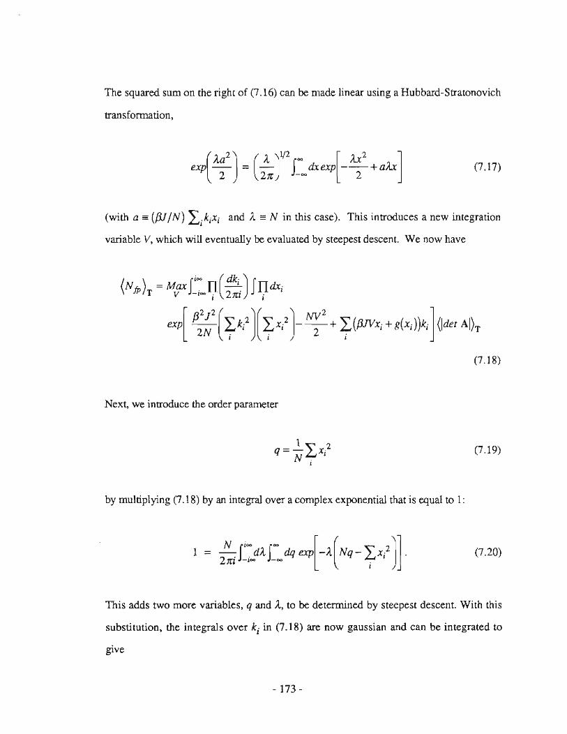
The squared sum an the right af (7.16) can be made linear using a Hubbard-Stratonovieh
transformation,
(7.17)
(with a '" ([31 IN) LjkjXj and A'" N in this case). This introduees a new integration
variable V, which wiil eventually be evaluated by steepest deseent. We now have
(7.) 8)
Next, we introduee the order parameter
q= ~LX? j
(7.19)
by multiplying (7.18) by an integral over a complex exponential that is equal to l:
l = ~fj~ dAf~ dq exp[-A(Nq - Lx?J] . 2m -j~ -~ . j
(7.20)
This adds two more variables, q and A, to be determined by steepest deseent. With thi s
substitution, the integrals over kj in (7.18) are now gaussian and ean be integrated to
give
- 173 -

(7.20)
Notice that the x/s on different sites i are now decoupled. This allows the N integrals
over the x/s to be written as a product of N identicai integrals. or as a single integral
over x (no index) raised to the Nh power.
We next consider the (Idet AJ)T' which we evaluate using the folIowing propert y of
the multidimensional gauss ian integral:
(7.22)
where Ai' i = l ..... N are the eigenvalues of A. and 9 is the step function.
e(z)=(I+Sgn(z))/2. Notice that the RHS of (7.22) equaIs det A as long as A is
positive definite, otherwise it equaIs zero. This is just what we need to count stable fixed
points: Recall that A is the Hessian of the Liapunov function for the dynamical systems
discussed above. Thus replacing Idet AI in (7.20) with (det A) TIi e[ Aj(A)] will pick out
the minima of the energy landscape. The RHS of (7.22) can be averaged by introducing
replicas [Bray and Moore. 1980], and eventually setting the number of replicas to -2.
Dropping the step functions (and understanding thatthe count now includes only stable
fixed points), we write
- 174-

(7.23)
Calculating the average over realizations (der Ah from (7.23) follows Bray and Moore
[1980], and is presented in Appendix 7 A. The result, which assumes replica symmetry,
is
(detAh'" Mjn I1(g'(xj)-2/iTR) exp(2NR2). ,
(7.24)
The Min over R comes from a steepest descent integral. Having to minimize with
respect to R (rather than maximize) is an anifaet af the replica method, as explained in
Appendix 7-A.
In cenain regions of state space {Xj}, the RHS of (7.24) becomes negative. We
interpret a negative result in (7.24) as indicating that A is not positive definite in that
region of state space, and that the rep lica symmettic treatment has failed to return a zero
for the average, as it should. Because we are interested in counting the stable fixed
points (where A is positive definite) we willlimit integrals over Slate space to the sub
region of the range of F where (g' (x) - 2f3JR) is positive . This is indicated by a n + n
marking such integrals. We note that limiting the integrals in this way was necessary to
obtain meaningful results from the saddle-point equations below.
From (7.21), (7.24), and the change af variables: B = -2f3JR, .1 = -f3.N, the
average number of fixed points can now be written
- 175-

(NfP)T = ~~ Mjn {exp[ N( ~~;:Z2 ÅQ+ln(I))]}
'" Max MB in {exp[Nå(J3,q'Å ,B,L1)]} q,Å.LI (7.25)
where
[
( )2 ] 1 g(x)-L1x 2 1= ~ J dx(g'(x)+B)exp 2 2 +.A..x .
27rq J3J + 213 J q (7.26)
and the + on the integral means "only integrate where (g'(x) + B) > O". Finding extrema
of (7.25) is done by setting derivatives of å(J3,q,Å,B,Ll ) to zero. This leads to the
folIowing set of coupled equations
då/dÅ =0 ::::) q = ((x2))
då/dL1 = O ::::) L1 = _1 ((x g(x))) 2q
då/dq=O ::::) Å = __ 1 (1 J32~2q (( (g(X)-L1x)2 ))) 2q
då/dB = O ::::) B=_J32J2(( (g'(x) + Bfl)) (7.27)
The double braekets in (7.27) indicate a weighted average, with the weight function
given by the integrand of I from Eq.(7.26):
(( ( )) = L dx f(x) W(x) .
f x) - J ' dx W(x) +
- 176-
(7.28a)
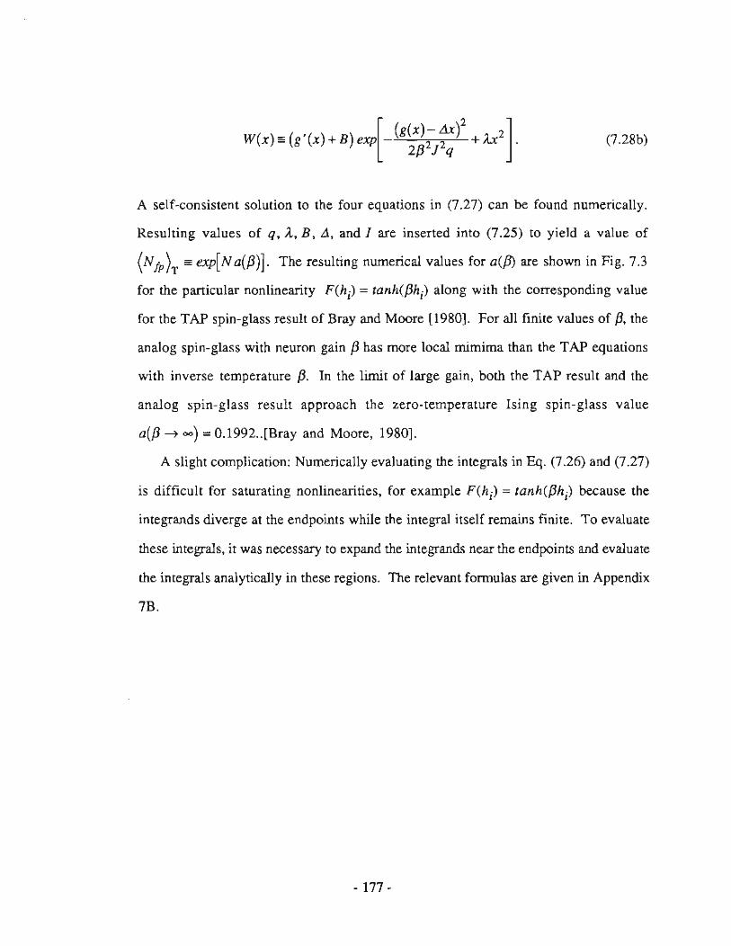
W(x) .. (g'(x) + B) exp[ (g(x)- LUl + }.x2]. 2/32 J2q
(7.28b)
A self-consistent solution to the four equations in (7.27) can be found numerically.
Resulting values of q, Å, B, .6, and I are inserted in to (7.25) to yield avalue of
(Nfp)T .. e.xp[Na(/3)J. The resulting numerical values fora(f3) are shown in Fig. 7.3
for the particular nonlinearity F(h j ) = tanh(/3h j ) along with the corresponding value
for the TAP spin-glass result of Bray and Moore [1980]. For all finite values of /3, the
analog spin-glas s with neuron gain f3 has more local mimima than the TAP equations
with inverse temperature /3. In the limit of large gain, both the TAP result and the
analog spin-glass result approach the zero-temperature Ising spin-glass value
a(/3 ~ 00) = 0.1992 .. [Bray and Moore, 1980].
A slight complication: Numerically evaluating the integrals in Eq. (7.26) and (7.27)
is difficult for saturating nonlinearities, for example F(h j ) = tanh(f3h j ) because the
integrands diverge at the endpoints while the integral itself remains fini te. To evaluate
these integrals, it was necessary to expand the integrands near the endpoints and evaluate
the integrals analytically in these regions. The relevant formulas are given in Appendix
7B.
- 177-

0.2 ,-~----r--~-...,-------r----r--.....,
analog spin glass
/ TAP spin glass
a(jJ)
0.1
0.0 L-~_-,-_~----,---==~-,-_~::::d
0.0 0.2 0.4 0.6 0.8
1/f3
Fi~. 7.3. Theoretical result for the scaling exponent a(f3) as a function of inverse neuron gain 1/f3 for the analog spin glass. The expected number of local minima is
(NIP) ~ exp[ a(f3)N j. Also shown for comparison is the number of solutions of the TAP equations at temperature l/Ø from Bray and Moore [1980].
- 178-

7.2.2. Analog neural network
In this section, we calculate the average number of local minima in the energy
landscape for an analog neural network as a funetion of neuron gain f3 and the ratio a
of stored memories to neurons. This ealculation [Waugh el al., 1990] is a hybrid of the
methods used in the previous section - which were originally developed by Bray and
Moore [1980] for the TAP spin-glass [Thouless et al., 1977] - and the analysis by
Gardner et al. [Gardner, 1986; Bruce et al., 1987] of the number and distribution of
fixed points in a Hebb-rule neural network with binary (Ising) neurons. We will not
consider how the fixed points are distributed in state space, but will instead eount their
total number. Based on Gardner's results, we expect that most of the fixed points have a
vanishing overlap with any of the memory pattems as N ~ 00. That is, most of the fixed
points are completely spurious states.
The analysis begins just as in the previous section, except that now the
interconnection matrix T = {Tijl is given by the Hebb rule:
i, j = l, ... , N. (7.29)
where eaeh ~; = ±l at random with equal probability and aN is the number of stored
patterns. The normalization (N -fa t l is ehosen to make I./ij - 1, independent of N
and a.
As in the previous section, the expected number of fixed points is found by
integrating a produet of delta functions on Gi over state space,
- 179-

(7.30)
with g(x) defined in (7.5) and A, the Hessian of the Liapunov funetion, defined in
(7.8). We use an integral representation of the delta function, this time taking k; real,
which gives
(7.31)
We now make the approximation that det A can be averaged separately from the rest of
the integral in (7.31). That is, we set the average of a product equal to the product of the
averages: (X x det A) = (X) x (det A). Physically, this procedure assumes that the vast
majority of local minima have identieal local eurvatures, so that a single value - the
average - ean be used as the multiplier for eaeh. This assumption is reasonable in light of
the faet that other features of the local minima, sueh as their energies and overlaps with
the stored pattems, behave in this way, i.e. their distributions are dominated by a single
value at large N. The only term in (7.31) whieh depends on the ~r -besid es det A -
is the second term in the exponential, whieh we write as
This term ean be further "simplified" by separating the produet on the right of (7.32) and
- 180-

introducing two new integration variables for each Jl. This replacement uses the double
Fourier integral:
1 f~ f~ exp[-i(AB)] = - da db exp[i(ab- Aa - Bh)]. 2.rr _ 00 _00
(7.33)
Rearranging slightly, (7.31) can be written
(N ) =f- rr(dk;) Irrdx;f- rr(dalldbll ) x fp ~ -~ . 21r . -~ 21r , , Il
eXP[<~::'k;(g(X;) + f3{ax;)+ i~allbll ] x
(exp[ -{N~ r t (all k; + bl'xj )sf ]) ~ (Idet AI)~ (7.34)
For sf = ± 1 with equal probability, the average over sf can be done easily,
(7.35)
where the term corresponding to a in (7.34) is « 1 for large N. Applying (7.35) to
(7.34) gives
- 181 -

(Idet AI)~ (7.36)
We now define three order parameters, q, s, and t, and their conjugate fields Q, S,
and T via integral defmitions of l:
1 1 = (N/2Jri)fI dqdQ exp[ Q(Nq- tX/)] q= N I, x? ~
, (7.37)
l 1= (N/2Jri)ff ds dS exp[s(NS- tk?)] s= - I,k.2
~ N . ' , (7.38)
t=~ I,xk ~ 1 = (N/21ti)ff dldT exp[ T(Nt - itX;k;)] N . " , (7.39)
This allows the integrals over aJl and bil in (7.36) to be evaluated by straightforward
gaussian integration, giving
- 182 -

(N fp ) ~ = (;:.S J dq dQ ds dS dulI' ap[ NG] x
r~If(~;) JIfdx i eX+tki(g(Xi)+(øra -T)Xi)] x
exp[ -QtX? -Stk?] (Ider AI)~ (7.40)
where
(7.41)
Beeause q, s, and t now only appear in the exp[NG] term, integrals over these
variables ean be evaluated easily using steepest descent by setting partial derivative s of G
equal to zero,
which yields solutions
2Sa q = 4QS+T2
()G=()G=aG=o, aq as ar
2Qa s - --=--.".
- 4QS+T2 Ta
t----" - 4QS+T2
(7.42)
(7.43)
(7.44)
The integrals over kj are now in gaussian form and ean be evaluated using (7.17), to
- 183 -

give
(N fp) = Max {( bJN exp[N(a- T.Jfi - a Itl( fJ2a 2J)] x
~ Q.S.T v47l'S f3 2 4QS + T
[ ( )2]1 g(x.) + fJ.Jfi - T x
fIldxi exp L -Qx? - I ( ) , (Idet AI)~ I i 4S
(7.45)
where Max indicates that the integrals over Q, S, and T are evaluated by steepest
descent by nurnerically maximizing the expression in curly brackets.
Calculating (Idet AI) ~ is done in a similar manner as for the analog spin glass: We
stan with (7.23), which picks out only the stable fixed points (the subspace where A is
positive definite) and average using the replica method over realizations of the Hebb
maoix. Again, we drop the absolute value brackets, as (7 .23) is only applicable where
del A > O. This rest of the calcularion is shown in Appendix 7C. The replica
symmetric solution is
(7.46)
where g'(x;) is the derivative of g(Xi} with respect to xi' As we discovered for the
analog spin glas s, the RHS of Eq. (7.46) becomes negative in cenain regions of state
space. Again, we exclude such regions from all integrations over state space. This
provides an approximate way of counting only the stable ftxed points, as described in the
previous section. Resoicting the domain of integration in this way was also necessary in
- 184-

order to obtain meaningful results from the saddle-point equations below. Substituting
(7.46) into (7.45), and changing the variables Q, R, S, and T to a new set: A, B,
q, and LI, by the definitions
gives
where
B == f3.J(i - 2R
A==-Q
q == 2S/f32
LI == T - f3.J(i
== Max Min {exp[N a(a,f3.q .A,B,LI)]} q,Å,<I B
(7.47)
(7.48)
i = -.J l f dx (g'(x)+B) exp[- (g(X)~LIx)2 +Ax2J (7.49) 2nq f3 + 2f3 q
and the "+" on the integral means that the region of integration is restricted to the range of
F where (g'(x) + B) > O. Notice that i from (7.49) is identicai to l from (7.26) upon
setting J = I. The rest of the present solution, Eq. (7.48), also bears a slTong
- 185 -

resemblance to the corresponding analog spin-glass solution, (7.25), but has some
significant differences. We note, however, that as a ~ 00, å(a,f3,q,Å,B,L1) ean be
expanded to the leading order in a and becomes identical to å(f3,q,Å,B,L1) from Eq.
(7.25). That is, in the limit a ~ 00 the analog Hebb-rule network is formaIly equivalent
to the analog spin glass. This eorrespondence has been noted aIready for the case of
binary neuron s [Gardner, 1986; Treves and Amit, 1988].
To find extrema of (7.48) with respeet to q, Å, B, and L1, we set partial
derivatives of å(a,f3,q,Å,B,L1) equal tozero,
aa _ aa _ aa _ aa _ O aq - (JÅ - aB - aL1 -
which gives a set of four integral equations:
q = (<1 +.Ja:~2-2Af32q ((x2))
O = af32 +((L1 +.Jaf3)2 -2Å{32q)[ (;g~:)) -1]
B = (~-f32)(( (g'(X)+Br1
))
Å = _[(<1 +~:~2~2Af32q ](I-tk(( (g(x)_L1x)2 )))
(7.50)
(7.51)
where, as above, the double brackets are a weighted average with the weight funetion
given by the integrand of j. The weighted average is exactly that given in Eq. (7.28),
setting J = 1 in (7.28b). For given values of a and f3. a set of solutions for q, l,
B, and L1 are found by numerieally solving (7.51). These four values are then inserted
into (7.48) to yield a numerical value for the quantity ofinterest, a( a,f3), defined as
- 186-

(7.52)
Notice that the tenns within the double brackets in (7.51) are identical to those appearing
in the spin glass analysis, Eg. (7.27). Thus to evaluate the integrals implied by the
double brackets we again must use the expansion of Appendix 7B.
Values for a( a,f3) are plotted in Fig. 7.4 for the particular case F(h) = tanh(f3hi).
The data show that for any value of the storage ratio a, the number of fixed points in the
energy landscape is reduced as the neuron gain is lowered. In the large-gain limit,
a(a,oo) is found numericaIly to agree with Gardner's [1986] result for binary neurons.
The fonn of (7.52) indicates that the number of fixed points is dramatically affected
by even small changes in a( a,f3), especiaIly for large N. As an example, consider the
effect of lowering the neuron gain from f3 = 100 to f3 = 10 in a network with storage
ratio a=O.I: Using the values a(O.l, IOO) =0.059 and a(O.l,lO) = 0.040, we expect
that the average number of fixed points will be reduced by - 97% for N=200 and by
eight orders of magni tude for N= 1 000.
7.3. COUNTING ATTRACTORS: NUMERICAL RESULTS
7.3.1. Technique for counting fixed points
The analyticaI resuIts of § 7.2, summarized in Figs. 7.3 and 7.4, have been tested for
the standard sigmoidal nonlinearity F(hi) = tanh(f3h) by directly counting the stable
fixed points in small computer-generated analog spin glasses and neural networks.
Numerical data were obtained by the folIowing procedure: At several values of f3 for the
spin glass, or pairs of values (a,f3) for the neural network, 20 random connection
- 187 -

100
100
'. '. '.
10
I l a
1
0.1
0.01 o
". '.
'. '.
0.2
0.01 O
. '.
'. ' .
".
. •...........•....•.......
0.4 0.6 1/f3
0.8
Fig. 7 .4. Theoretical result for the scaling exponent a( a,{3) as a function of inverse neuron gain 1/{3 and inverse storage ratio l/a for the analog Hebb-rule associative memory. The expected number of flxed points is (NIP) '" e.xp[a( a,{3)N] .
- 188-
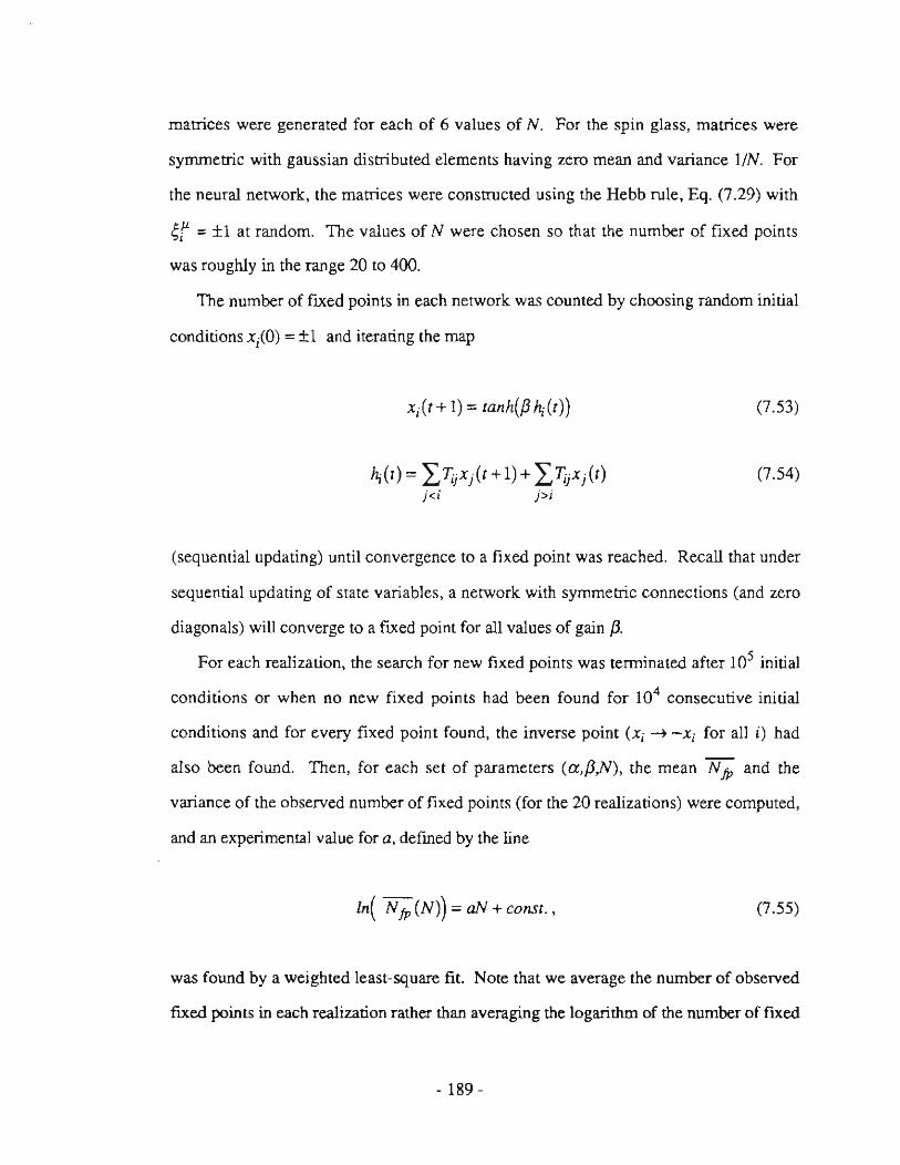
matrices were generated for each of 6 values of N. For the spin glass, matrices were
symmetric with gaussian distributed elements having zero mean and variance liN. For
the neural network, the matrices were constructed using the Hebb rule, Eq. (7.29) with
sf = ±l at random. The values of N were chosen so that the number of fixed points
was roughly in the range 20 to 400.
The number of fixed points in each network was counted by choosing random initial
conditions xj(O) = ±l and iterating the map
Xj(t+ I) = tanh(/3 h; (t)) (7.53)
(7.54) j<; j>i
(sequential updating) until convergence to a fixed point was reached. RecaU that under
sequential updating of state variables, a network with symmetric connections (and zero
diagonals) will converge to a fl.Xed point for all values of gain /3.
For each realization, the search for new fixed points was terminated af ter J05 initial
conditions or when no new fixed points had been found for 104 consecutive initial
conditions and for every fixed point found, the inverse point (Xj -t -Xi for all i) had
also been found. Then, for each sel of parameters (a,{3,N), the mean N fp and the
variance of the observed number of fixed points (for the 20 realizations) were computed,
and an experimental value for a, defined by the line
ln( Nfp(N))=aN+const., (7.55)
was found by a weighted least-square fit. Note that we average the number of observed
fixed points in each realization rather than averaging the logarithm of the number of fl.Xed
- 189-

points. This coincides with the analysis above: recall that in § 7.2. we calculated
in(N fp)' not (in(N fp )). As we have argued. the two types of averages are expected to
agree in the large-N limit for the fully connected network.
7.3.2. Numerical resuIts for analog spin glass
Numerical resuIts for the analog spin glass. obtained using the above procedure. are
shown in Figs. 7.5 and 7.6. Notice that the data in Fig. 7.6 agree quite well with the
analyticaI result for the analog spin glass. but are quite different from the TAP result of
Bray and Moore [1980]. To our knowledge. there are no comparable data verifying the
Bray and Moore curve away from T = 1If3 = O. This is due. in part. to the chaotic
dynamics exhibited by the dynamical version of the TAP equations [Bray and Moore.
1979]. In particular. since few initial conditions terminate at fixed points for the TAP
equations at finite f3. it is extremely difficult to count fixed points numericaIly in even a
single realization5.
7.3.3. Numerical resuIts for the neural network
Fixed point counts for the Hebb-rule neural network were performed at six points in
the (a.f3) plane. Results are shown in Figs. 7.7 and 7.8. In Fig. 7.8. the numerical data
are presented along with the analyticai resuIts for a = 10. 1. and 0.1. The agreement is
very good at larger values of a and f3. and reasonably good - though oUlside the range
of the error bars - for smaller a and f3.
It is not clear why theory and numeries disagree for a( a.f3) <- 0.05. At small a.
5 Nemoto and Takayarna [1985] claimcd IO be investigating just thi s problem using a variation of the TAP equations which is guaranteed IO converge and which has as its solutions a superset of the solutions of the TAP equations. Apparently. this work has not been published.
- 190-
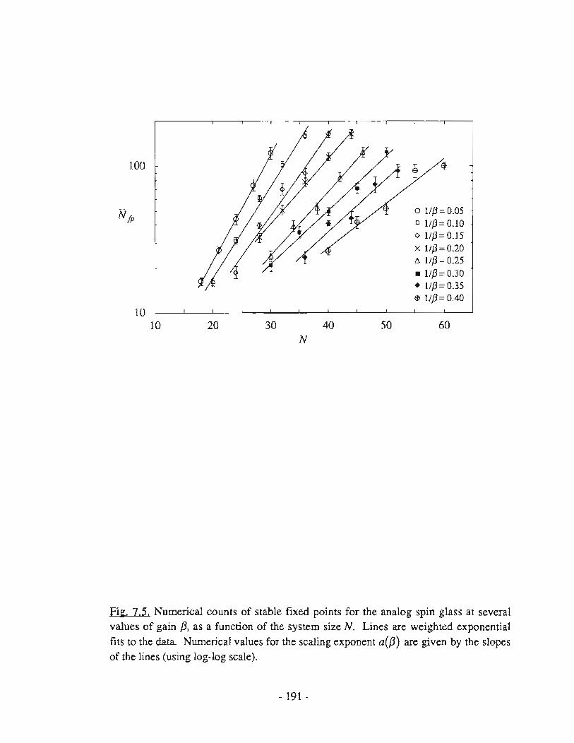
100
10 10 20 30 40 50
N
o 1/{3= 0.05 c 11{3= 0.10 o 1/{3= 0.15 x 1/{3=0.20 tJ. 1/{3= 0.25 • 1/{3= 0.30 • 1/{3= 0.35 El> 1/{3= 0.40
60
Fil:. 7.5. Numerical counts of stable fixed points for the analog spin glass at several values of gain /3. as a function of the system size N. Lines are weighted exponential filS to the data. Numerical values for the scaling exponent a(/3) are given by Ihe slopes of Ihe lines (using log-log scale).
- 191 -
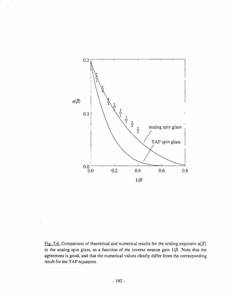
0.2 ,....-~----,-~-..,------,-~--,
2 analog spin glass
/ T AP spin glass
o.o~' -~-"--~-----'--=~--"----~~
0.0 0.2 0.4 0 .6 0.8
1/f3
Fig. 7.6. Comparison of theoretical and numerical resuIts for the scaling exponent a(/3) in the analog spin glass, as a function of the inverse neuron gain 1//3. Note that the agreement is good, and that the numerical values clearly differ from the corresponding result for the TAP equations.
- 192-
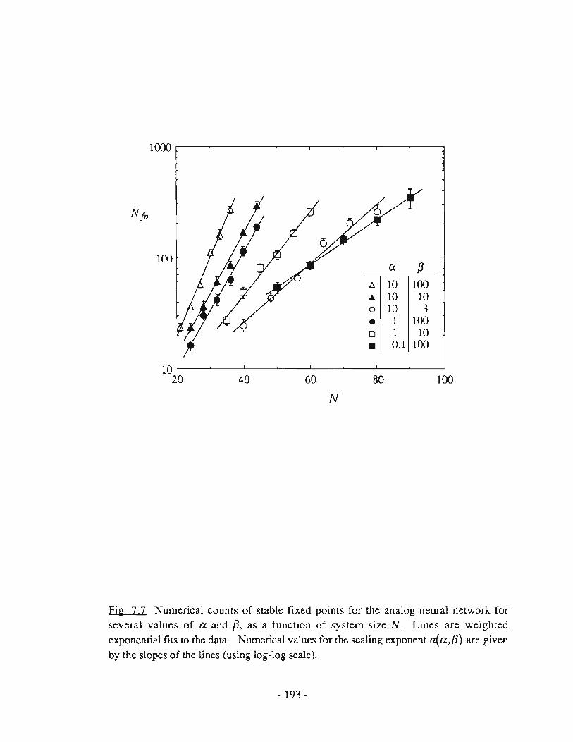
1000,--------,--------,--------,-------,
100 a {3
'" 10 100
'" 10 10 o IO 3
• 1 100 D 1 10
• 0.1 100
10 20 40 60 80 100
N
Fifl: 7 7 Numerical counts af stable fixed points for the analog neural network for severa1 values af a and {3, as a function af system size N. Lines are weighted exponential fits to the data. Numerical values for the scaling exponent a(a,[3) are given by the slopes af the lines (using log-log scale).
- 193-

0.2 ,-----,---- --r----.-------,
0.15
a( a,f3)
0.1
a=10
0.05 + a=1
a=O.l
o L-_ _ _ ~ ___ ~ ____ L-___ ~
o 0.1 0.2 0.3 0.4
1If3
Fig. 7.8. Comparison of theoretical and numerical results for the scaling exponent a(a,{Jl in the analog associative memory. The agreement is good, especiaIly at larger values of a and {J.
- 194-
the problem ean likely be traced to the assumption in the analysis that N{(i » I, while
numerical data for a = 0.1 are limited to the range IS < N{(i < 30. Why smaller values
af /3 should also cause problems - even for large a and for the analog spin glass - is
unknown.
7.4 DISCUSSION
7.4.1 Asymmetry - An alternate way to eliminate spurious aUraclors
We have shawn analytically and numerically that lowering the gain af the neuron
transfer function in an analog spin glass or neural network greatly reduces the number af
local minima in the energy landscape. This phenomenon provides one rnechanism for the
observed improvement af performance in analog neural networks compared to their
binary-neuron counterparts. Because the present method af smoothing the landscape is
fully deterministic , it ean be implemented in electranic hardware much more easily than
stochastie methods sue h as simulated annealing.
An altemate strategy for deterministieally eliminating the spurious ("glassy") fixed
points in a neural network is to add same degree af (quenehed) asymmetry to the
eonneetion matrix. This idea has been considered by several authors [Parisi, 1986; Hertz
et al., 1987; Crisanti and Sompolinsky, 1987; Treves and Amit, 1988; Kepier, 1989].
In a deterrninistie Ising spin glass, for example, asymmetry reduees the number af fixed
points (Fig. 7.9a) as well as the total number af attraetors (Fig.7.9b) [Gutfreund et al.,
1988]. For the fully asymmetric spin glass (k = 1 in Fig. 7.9), the number of fixed
points is no longer exponentially inereasing with N, and the total number af attraetors is
minirnized.
- 195-

0.2 --=-------------(a-j---,
• 0.1
. -"
o 0.2 O_l. 0_6 0_8 LO
k
30 Ibi
20
10
O 0.2 o l. 0.6 0.8 1.0
k /l k.l l
Fig 79 (a) Scaling exponent a(k) for fixed points and as a function af asymmeu-y parameter k for asymmetric spin glas s with binary (Ising) state variables and sequential dynamics. Conneclion matrix is composed of gaussian random symmetric and antisymmetric pans, ~j = ~J + k~t . Line is theory, squares are from numerical counts. (b) Numerical counts of the total number af attractors as a function of asymmetry for various size systems. Both the number of fixed points and the total number of attractors can be reduced by introducing asymmetry, but this also introduces non-fixed-point attractors. After Gutfreund et al.[1988].
- 196-
In the limit N -> 00, all attractors of finite period disappear entirely; the only dynamical
state for the fully asymmetric analog spin glass (besides the origin at low gain) is chaos
[Sompolinsky et al., 1988].
Treves and Arnit [1989] have studied the distribution of fixed points in Hebb-rule
neural network (with binary neurons) for arbitrary symmetry and dilution. They find
that, in contrast to the spin glass, a neural network at finite a has an exponential number
of fixed-point attractors for all values of asymmetry - including full asymmetry. Kepier
[1989] has taken an additional step to eliminate these remaining spurious fixed points by
adding a self-inhibition term Tii < 0, which eliminates fixed points, and (for parallel
dynamies) creates in their place period-2 limit cycles. Kepier's result, as well as Fig.
7.9, highlights an imponant drawback of smoothing with asyrnmetry: Using asymmetry
to reduce the number of [ued point attractors necessarily creates new, nonjixed·point
attractors. In contrast, smoothing the landscape using analog neurons eliminates fixed
point attractors without introducing any new attractors.
7.4.2. A short discussion of attractors in multistep systems
Finally, we will briefly discuss the nature of the attractors in the multi step updating
mie defined in Ch. 6. We will restriet our attention to the binary (Ising) spin glass (Tjj
gaussian random symmetric), and compare a sequential update scheme to the M= 2
updating rule, where state variables are updated in parallel based on the average of two
previous time steps. We expect that our observations will be qualitatively correct for
analog systems and neural networks.
First - to check the validity of our numerical method owe reproduce the well-known
result that the Ising spin glass under single-time-step sequential dynamics always
converges to a fixed point and that the expected number of fixed points is
- 197 -

(NIP) = exp[aN] with a = 0.1992 ... [Tanaka and Edwards, 1980; De Dominicis et
al., 1980; Bray and Moore, 1980; Gutfreund et al., 1988]. This result is shown in Fig.
7.10. The numerical method is similar to the one described above: Here, 40 random
gaussian matrices were generated for each value of N with 8 S N S 18. For each
matrix, random initial states (random N-vectors of ±I's) were generated and their
associated anractors were found using sequential dynamics:
Xi(t + l) = Sgn[~TijXj(t + l) + ~1ijXj(t)] . ) <, j >'
(7.56)
Fixed points for each matrix were counted and tabulated. A particular matrix was
considered fully mined for attractors when 500 consecutive initial states were tested
without finding a new attractor. (This occurred af ter anywhere from 502 to several
thousand initial states had been examined). The numbers of fixed points for each of the
400 matrices were plotted and a direct, least-square exponential fit to all 400 points was
made (using KaleidaGraph 2.0) to find the scaling exponent a. This method of
averaging is not the same as finding the average number of fixed points for each value of
N first, and then doing an exponential fit. The two methods, however, yield very
similar results. The least-square fit gives a = 0.2030, within 2% of the theoretical value.
Now we tum to the M = 2 multi step update rule. Recall that in § 6.2.2 it was proved
that all attractors for this update rule (with symmetric connections) are either fixed points
or period-3 limit cycles. This resuIt is supponed by the present numerical investigation.
Counts of fixed points and 3-cycles are show n in Fig. 7.11. The fixed points and 3-
cycle were counted by the same method described above (40 matrices for each N, 8 S
N S 18 and 4 matrices for N = 19). In this case, initial states were generated until no
new attractors of either type had been found for 500 consecutive initial conditions.
- 198 -
Because there were typically a large number of 3-cycles, this often meant checking tens
of thousands of initial conditions per matrix. Care was taken not to overcount 3-cycles
that are identicaI under cyclic permutation, though noncyclic permutations were counted
as separate attractors. We point out three important features of the data in Fig. 7.11 :
(1) The scaling exponent for the number of stable fixed points using 2-step dynamics is
significantly below 0.1992. The measured value is afp = 0.175.
(2) The scaling exponent for stable 3-cycles is larger than that of the fixed points (for
either type of dynamics), and is measured to be a3-cyc = 0.237. Thus 3-cycles are quite
abundant in the 2-step network - much more so than fixed points. On the ether hand, the
3-cycles are not as abundant as the 2-cycles generated by standard (M = l) parallel
updating, which are known to have a scaling exponent or a2.cyc = 2(0.1992) = 0.3984
[Gutfreund et al. , 1988, Cabasino et al., 1988).
(3) The number of 3-cycles seems not to be self-averaging. For a given system size,
the number of 3-cycles found in particular realizations varies by up to two orders of
magnitude, with (Ni:' - Nj}n)j NIp - 0(1).
- 199-

fit: Y = 0.94 exp(0.203x) 100
sequential dynamies o
• o ! I
NfP o o o o o § o
o o o o
o o o o 8 8 10 o o o o o o o o o o o
o o o o o o
o o o o o o
o o •
l 6 8 IO 12 14 16 18 20
N
Fig. 7.10. Number of fixed points Nfp as a function of system size N for the Ising spin glas s with single-step sequential dynamics. See text for detaiis of the numerical method.
The direct exponential fit to all 400 points (line) gives a scaling exponent of a = 0.203,
in good agreement with the theoretical value of 0.1992.
- 200-

(a) fit: y : 1.19 exp(0. 175x) 100
2-step parallel dynamics o
Nfp
§ o o
~ o o
8 10 8 o g . • o o o o o o o o o
o • . o o o o
o o o o o o o o o o
o o o o
1 6 8 10 12 14 16 18 20
N (b)
lil: y : 2.25 exp(0.237x) 1000
2-step parallel dynamics o o
8 o i o o
i ~ o 8 o o o • o • B •
o o o o • o 100 o I
,
8 o
N o 9 o
I • o • o 3-eye 9 o o
li o o o
~ o o
10 § o B o
o o g o o , o o o o
o o o o o o o o
o o
I 6 8 IO 12 14 16 18 20
N
Fig. 7.11 . Number of fixed points Nfp and distinct 3-cyc1es N 3-eye as a funetion of system size N for the Ising spin glass with 2-step parallel dynamics (see § 6.6.2). See text for details of the numerical method. (a) The numerically determined fi xed-point scaling exponent is afp: 0.175. This value is signifieantly less than the sequential update value of 0.1992 (see Fig. 7.10). (b) The numerieally determined 3-cycle scaling exponent is a 3-eye : 0 .237. This value is larger than afp ' so at large N the vast majority of attractors for the 2-step spin glass are 3-cyc1es.
- 201 -

APPENDIX 7A: (der Ah FOR THE ANALOG SPIN GLASS
In thi s appendix we calculate the average (over realizations) of the determinant of the
Hessian matrix A, defined in Eq. (7.8). The method follows Bray and Moore [1980].
Replieas were inrroduced in the main text; we piek up the calculation starting at Eq.
(7.23).
From Eq. (7.23), the average overrealizations is given by
(7 A.l)
Writing the average in (7 A.l) as an integral over the gaussian distribution of matrix
elements (7.6),
{ ( ) 1/
2
[ ()] . ~ dPia ~ N N 2
(der Ah = LIm L IT = L ITdT;j --2 exp I. - ~ 7;j X m-->-2 ~ i.a -v 2n ~ (ij) 21t.l (ij) 2J
(7 A.2)
with (ij) indicating distinct pairs. Integrals over Tij are gaussian and ean be integrated
to give
- 202-

(7 A.3)
where now the double sums over i and j are unrestrieted. The squared sum ean be
redueed using a Hubbard-StralOnovieh transformation (7.17), whieh introduees !Wo new
order parameters, an m-eomponent veetor R a and an m x m matrix M afJ '
exp[ (J:~2) t ( ~PwPja J] = exp[ J:~2 ~( ~>ia 2 J] exp[ J:~2 a~J ~PiaPiP J] = (cermA)(tennB) (7 A.4)
where
(7 A.5)
(7 A.6)
FolIowing Bray and Moore [1980], we adopt the repliea symmetrie solutions Ra = R for
- 203-

all a, and M (lP = O for all (a,p>, which reduces (7 A.S) and (7 A.6) IO
1/2 []m (termA)=(~) CdR exp(-NmR2) exp J/3Rt Pia2 , (7A.7)
(rermB) = 1.
mserting (7 A.7) imo (7 A.3) gives
(7A.8)
mlegrals over Pia are now gaussian and ean be inlegrated to give
(der Ah= m~~2 {r .. dR( ~r exP[-NmR2 1[ ~(g'(Xi)- 2/3JRr1/2 r} = r .. dR(~r exp[2NR21 ~(!?'(x;)-2/3JR). (7A.9)
The imegral over R in (7 A.9) is eventually done by steepest descent. Because the
number of replicas has been set to -2, the correct solution of this steepest decem integral
tums out to be a minimum over R, rather than a maximum. This is also the case in the
analysis of Bray and Moore [1980] as they use the solution B = 0, which is likewise a
minimum of det A. Neglecting numerical prefactors of 0(1), we obtain the folIowing
result:
- 204-

(7A.I0)
which appears as Eq. (7.24).
APPENDIX 78: EXPANSIONS FOR STEEPEST DESCENT INTEGRALS
Finding a solution of the sad dIe-point equations for the analog spin glass (7.27) or
the analog neural nerwork (7.51) requires solving a set offour coupled equations, each of
which contains an integral in the fonn of the double angle braekets defined by (7.28).
These integrals, five in total, must be evaluated numerically . For the analog transfer
function F(h j ) = tanh({3h j ), four out of the five integrands diverge at the end points of
the domain of integration, ±I, causing fatal problems for the numerical integration
package used (NAGLIB 001 AHF). To get around this problem, we split the domain of
integration into three regions:
J1 J-I+' JI-' Il -l = -l + -IH + l-c
(7B .l)
which can be evaluated as
JI JI-C rI -I = -I+c + 2 Jt-, (7B.2)
by vinue of the (even) symmetry of all of the integrands. The integrals with limits at
±(l-e) no longer have divergent integrands over this reduced domain, and ean be
evaluated accurately using the NAGLIB integration package. The remaining parts,
extending over [1-e,I], ean be approximated for e « l, keeping only those terms
- 205-

which diverge as x ~ 1. Once nonleading tenns are dropped, the [1-1",1] integrals can
be evaluated in closed form, giving expressions which depend on e. The procedure is
straightforward, and we give only the results. The approximations were checked by
comparing several values of e, ranging from 10-4 to 10-8, and confirming that the sum
of the two integrals on the right of (78.2) was insensitive to the choice of e, though the
individual parts of each integral did depend on e.
We have suppressed the "+" markers on the integrals indicating that the range of
integration is limited to a sub-region where (det A) > O. The excluded region is in the
center of state space - covered by the "easy" integral over [-1+1", l-e] which is done
numerically.
First, we consider the integral j of the weight function W(x) defined in (7.28b) for
the case of the neuron transfer function F(hi) = tanh({3h):
- Jl 1= dxW(x) -)
(78.3)
W1xl=C_'" +B 1""'[ (7B.4)
Notice that j is proponionalto the I's defined previously: i = [..j27rq {3J]/ from (7.26)
and i = [-J27rq {3]i from (7.49). Expanding (7B.3) near ±l as descibed above gives
- Jl-o b-f7i Å l:: dxW(x) + -e ettc[ajb) , -IH 2
(78.5)
where
- 206-

a = !n(2/e) - 2t1,
b = 2f31..j2q ,
and erfc is the complementary error function,
2 f~ _/ 2
erfc( z) '" ..fii z dt e .
(7B.6a)
(7B.6b)
(7B.7)
U sing these same definitions of a and b, the integrals in double braekets from (7.27)
and (7.51) have the folIowing expansions:
(( X 2)) '" J 5~1 dxx2
W(x)
::1[51-< dxx2 W(x) +
l -1+<
(( x g(x»)) = J C dx (x tanh -1(x») W(x)
b..fii .1. ] -2-e erfc[a/b] ,
:: 1[51-< dx(xtanh- 1(x»)W(x)
l -1+<
+ e: (%exp(_a 2/b2) + t1..fii erfC(a/b»)]
(( g(x) - t1x)) '" J fl dx( tanh -1(X)_ t1x)W(x)
::1[51-< dx(tanh-1(x)-t1x)W(x)
l -IH
+ (%f e.1.( (: )exp(-a2/b
2) + ~ erfc(a/b»)] .
- 207-
(7B.8)
(7B.9)
(7B.lO)
Finally, the integrand in (( (g'(x) + Bt )) does not blow up at ±I for F(h) =
tanh(f3hi), so it is not necessary to expand the integrand in arder to numerically evaluate
this integral.
APPENDIX 7C: (det A)~ FOR THE ANALOG NEURAL NETWORK
In thi s appendix, we deri ve the expression (7.46) for (del A)~, the average
determinant af the Hessian matrix A, defined in (7.8). The average af det A is taken
over realizations af Hebb matrices, defined in Eq.(7.29), each storing aN unbiased and
uncorrelated random memory patterns. That is, each ~f', i = l, ... , N; 11= l, ... , aN
in (7.29) equals ± 1 at random.
We start with the identity (7.22),
(7C.1)
and introduce replicas, indexed by r, with the number af replicas eventuaIly set to -2,
- . J- dPiy (I ~ ~ J det A - L/m __ IT ~exp --~ ~PiyAijPjr . m->-2 i yv2lC 2.. I
• I.J r= (7C.2)
As with the analog spin glass, we drop the absolute value braekets around the
determinant, recognizing that (7C.l) is nonzero only when A is positive definite, which
implies det A > O. The cIaim that (7C.2) picks out only the stable fixed points after
averaging is ani y valid insofar as replica symmetry is valid. The validity af replica
symmetry in this problem wilI not be studied.
- 208-

We write the average over ~f as
. (f~ dPiy (1" ~ J~ (detA)~ = LIm _~n =exp --~ ~PirAijPjr m->-2 i Y ,,271: 2 . . l
• I,j y= ~
(7C.3)
where the angle brackets denote an average over all 2 (J]oI2 slates of ~f'. Note in (7C.3) that averaging is done before the number of replicas is set to -2. Insening
Aij from (7.8) and Tij from (7.29) into (7C.3) gives
(der A) ~ = Lim (en d~ exp[-~ L Pi/(g'{X;) + ø..Ja) m .... -2 iy--v271: 2 . , I,y
I ø ( 1')2]\ +"2 N..Ja L LPiy ~i ) ~I' I ~
(7C.4)
The square in the last term of (7C.4) can be reduced to a linear form via a Hubbard-
Stratonovich transformation,
(7C.5)
[with),,= l and a = (ØIN..Ja)1/2Li~fpiY in this case]. This introduces a new set of
integration variables, (J'YJl (y= l, ... , m; Po = l, ... , aN) and gives
- 209-

J~ da,!!, J- dPir (derA), = Lim n = n = x
., m .... -2 -- '127r -- . '127r r,~ I,r
(exp[(N~ rI Piy a}!' ~t]) . (7C.6) ',y,~ ~
Averaging over the ~t' can now be done imrnediately using the relation
(7C.7)
The term eorresponding to a in (7C.6) is small for large N, so that the O(a4 ) terms ean
be dropped:
We now assume replica symmetry by sening a}!' = aJL and Piy = Pi for all y. This
allows (7C.6) to be written as a single-site integral (in replica space) raised to the power
m:
(7C.9)
- 210-
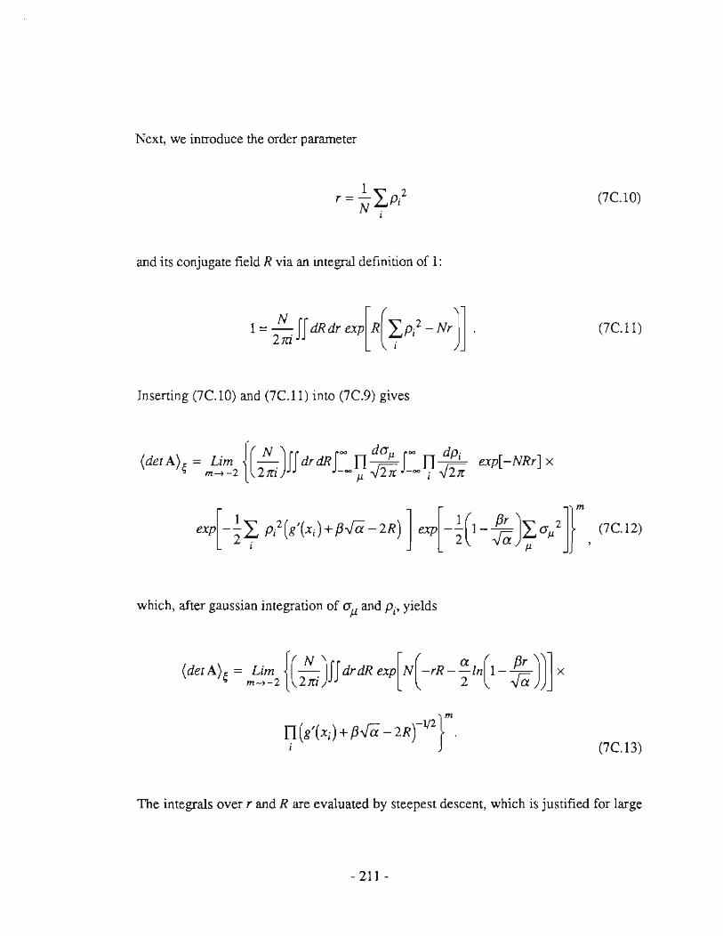
Next, we introduce the order parameter
l r=-~>?
Ni (7C.1O)
and its conjugate field R via an integral definition of l:
(7C.ll)
Insening (7C.1O) and (7C.ll) into (7C.9) gives
(detA)~ = Lim {(~)ffdrdRf~ n ..,ffiidap f~ n..,ffiidPi exp[-NRr] x • m .... -2 2m -~ 27r -~. 27r P ,
which, af ter gaussian integration of aJ1. and Pi' yields
(7C.13)
The integrals over r and R are evaluated by steepest descent, which is justified for large
- 211 -

N. Each integral produces a factor (2rr/N) 1/2 to cance! the existing prefactor
proportional to N. Other numerical prefactors of 0(1) will be ignored. The steepest
descent integral over r can be done explicitly by setting
.!...[rR + a ln(l- f3r/..J(i)] = O ar 2 (7C.14)
which gives
(7C.lS)
The steepest descent integral over R will eventuaIly be done numerically. Seuing the
number of replicas to -2 before performing the saddle point integral makes the minimum
(not the maximum) with respect to R the valid solution. lnsening (7C.lS) into (7 C. 13)
and setting m = -2 yields tlle desired result,
. { [(2..J(iR (detA)~ = ~n exp N f3
(7C.16)
which appears as Eq. (7.46).
- 212-

Chapter 8
TRE DISTRIBUTION OF BASIN SIZES
IN TRE SK SPIN GLAS S
8.1. INTRODUCTION: BACK TO BASINS
In this chapter, we return to the problem considered in Ch. 3, namely, the structure of
the basins of attraction in systems with a large number of atlractors. We restrict our
attention to the zero-temperature SK spin glass [Sherrington and Kirkpatrick, 1975J, and
study the distribution of basin sizes, averaged over the ensemble of (gaussian) random
connection matrices.
The dynamical system we consider is the SK model with deterministic, discrete-time
(sequential) dynamies:
Si(l+l)=Sgn[~"lijSj(/+I) + L "lijSj (l)] Jq J>I
i = I, ... , N. (8.1)
The state space of this system is discrete, Sj = ±1, equivalent to the eorners of an N
dimensional hypercube. Later in the chapter (§ 8.5) we will consider an analog version
of Eq. (8.1). The connection matrix T ={Tjjl is taken to be symmetric (Tjj = Tjj)
with off-diagonal elements drawn at random from a gaussian distribution P(T;) with
zero mean and variance liN,
- 213 -
(8.2)
and all Tii = O.
The main result of thi s chapter is that over a wide range of basin sizes W, the
numerically-measured distribution j(W) of basin sizes for Eq. (8.1) is roughly
described by a power law, j(W)= KW-r , with r - 3/2. (These quantities are defined
precisely below, see (8.4) and (8.7)). Af ter exploring some of the immediate
consequences of such a power-law distribution (§ 8.3), we will compare this resuIt to
known basin-size distributions for other systems, and to a closely related quantity defined
for the SK spin glass, the distribution of cluster weights (defined in § 8.4). Finally, we
show that using analog state variables selectively eliminates fixed points with smal!
basins as analog gain is lowered (§ 8.5). A discussion and open questions are presented
at the end (§ 8.6).
With all of the attention that has been paid to the SK spin glass over the past fif teen
years [Binder and Young, 1986; Mezard et al., 1987], it is surprising that a direct
measurement of basin sizes has not been presented previously. l Two explanations for
this lacuna seem likely: First, there is the well-known "universality" of systems with
multivalley energy landscapes [Derrida and Flyvbjerg, 1987a, 1987b; Gutfreund, 1988;
Derrida, 1988b]. This univers ali ty has prompted comparisons of different quantities in
different systems, all of which characterize state space in some way. For some models -
such as the Kauffman model (§ 8.4.2) - the quantity used for comparison is in fact the
IN. Parga and G. Paris i have studied a rclated distribution in the T=O SK model using a numerical technique very similar to ours. Rather than looking at the distribution of basin sizes, they mcasured the fraction of initial states that terminate at a fixed point with energy between E and E + t1E, as a function of E. They found that as the system becomes large, most initial states flow to fixed points with E/N - 0.7, with a rather narrow peak. Apparently, this work has not been published except as a preprint [Triest preprint IC/85/l33 (1985)). Some aspects of the work are discussed in Parga [1987J, and a figure from the preprint appears in the book by Chowdhury [1986. p. 82-83J.
- 214-

distribution of basin sizes. For the SK spin glas s, it is another quantity, the distribution
of cluster weights which is generally used for comparison. An exact expression for the
distribution of cluster weights has been presented and analyzed thoroughly [Mezard et
al. , 1984a; 1984b]. Our results for the SK model suggest that besides the important
concepmal difference between the distribution of cluster weights and the distribution of
basin sizes, there are also fundamental qualitative differences between these two
distributions. Our conclusion is that perhaps such distributions are not so universal, and
that care must be taken in making comparisons between them.
The second reason why this problem has not received more attention is that basins of
attraction can only be strictly defined for deterministic systems. Furthermore, their shape
can depend on the detaiIs of the dynamics. li is only recently that spin glasses have been
trealed as dynamical systems in their own right, and thaI the standard dynamical-systems
type questions have begun to be addressed [see, for example: Gutfreund et al., 1988;
Cabasino et al., 1988; Sompolinsky, 1988; Kanter, 1990].
8.2. PROBABILISTIC BASIN MEASUREMENT
FirSI, we note that all attractors of (8.1) are fixed points (this is nOl true for
asymmetric connections or parallel dynamics). This faet ean be established by showing
that the total energy, E (Le. the spin-glas s Hamiltonian)
(8.3)
is a Liapunov function of (8.1). In Eq. (8.3), E; is the energy eontributed by site i,
equivalent to the local field al sile j times -S/2. We will also refer to the average energy
per site, defined e == E/N. Intuitively, we expect that the most stable attractors (those
- 215-

with the most negative energy) will have the largest basins of attraction. lndeed, this idea
is observed to hold for the recaU states in associative memory models [Forrest, 1988;
Kepier and Abbotl, 1988; Opper et al., 1989], and is an important principle for
developing robust learning algorithms [Krauth et al., 1988; Abbotl, 1990]. The
numerically measured relationship between basin size and average energy per spin e for
the SK model (8.1) is shown for N = 20 in Fig. 8.1. This figure shows - 11,000 fixed
points from 200 realizations, and confirms the intuition that more stable fixed points have
larger basins of attraction. It is significant, however, that the dependence of basin size on
energy is quite weak: Fixed points with identicai energies have basin sizes ranging over
two orders of magni tude.
We now explain how Fig. 8.1 was made. Define the size W s of the basin of
attraction of the sID attractor as
= number of initial states leading to attractor s Ws
- total number of initial states (8.4)
TIlls definition satisfies the normalization
(8.5) s
Having only fixed point attractors greatly simplifies the task of measuring basins, since it
is always clear to which attractor a particular initial cOlJdition has flowed. Still, because
of the large state space ( 2N states for a system of size N ) a complete enumeration of
basin sizes is prohibitively time-consuming for all but the smallest systems (such an
approach was used by Gutfreund et al., [1988]). The problem is compounded by the
need to average over large numbers of rea1izations in order to obtain reliable statistics.
Instead, we compute basin sizes Ws by the folIowing probabilistic method. For each
- 216-

o
-0.2
-0.4
-0.6
-0.8
-I 0.0001 0.001
N=20
0.01 0.1 I
Basin size
Fil.:. 8.1 . Basin size versus energy per site t;; = E/N for fixed points in 200 realizations of the detenninistic SK spin glas s, Eq. (8.1) and (8.2). The number of data points, equal to the number of fixed points found using the statisticai technique, is 11 ,032. The relation Nfp = exp[aN] gives a = 0.200 for this data, in good agreement with the theoretical value 0.199. Each realization was checked for fixed points until 500 consecutive initial states failed to produce a new fixed point (see text). Note the general trend that the most stable fixed points (i.e. fixed points with the most negative IO) have the large basins of attraction. Also note that the trend is rather weak.
- 217-

realization of Tij' random initial states (random, unbiased strings of ±I 's) are generated,
and the attractor for each initial state is found under the dynamics of (S. 1 ). Convergence
is fast, typically requiring fewer than 5 updates per site. A list of the distinct attractors is
kept along with the total number of initial states that flowed to each attractor. For each
initial state, the attractor found is compared to the list of those previously found, and if
there is a match, the basin size of that match is incremented. If no match is found after
checking the entire list, the attractor found must be new. The new attractor is then added
to the list of attractors with its basin size initialized to l. For each realization of Ti}'
initial states are generated until a quitting condition is reached. The quitting condition is
that a specified number of consecutive initial conditions have been generated without
tinding a new attractor. Typically this number is set to 500 for N::; 20 and SOD for N >
20. This quitting condition is superior to simply using a large, fixed number of initial
conditions to test each realization; It is efficient over a wide range of possibIe numbers of
attractors withoUl requiring a good "guess" (i.e. a pre-inserted theory) for how Ion g to
sample. Af ter reaching the quitting condition, basin sizes for each of the found attractors
are given by the number of initial states that flowed to that attractor divided by the total
number of initial states tested. Statistics are accumulated over a large number of
realizations (typically 20D - 500).
There is a check which tells us if we have sampled long enough. We know the total
number of tixed points that we should find. The expected number of fixed points NIp
for (SJ) is
(8.6)
with A-I and a = 0.1992 ... [Tanaka and Edwards, 1980; De Dominicis et al., 19S0;
Bray and Moore, 1980]. (Henceforth we will drop A, calling it l, and drop the braekets
- 218 -

on Nfp indieating an average over realizations). The result (8.6) was originally
ealculated assuming large N, but it is remarkably aeeurate for N as small as N = 4 (!)
when averaging is done over a large number of realizations IGutfreund et al., 1988] .
The distribution of basin sizes ean be found numerically by selting up a histogram of
basin sizes, and collecting data over a large number of realizations. A histogram of basin
sizes for the 11,000 points of Fig. 8.1 is shown in Fig. 8.2(a). Figure 8.2(b) shows a
histogram of energies per site t: for this same data set.
8.3 THE DISTRIBUTION OF BASIN SIZES
8.3.1. Definitions
The distribution of basin sizes, averaged over realizations, ean be written as a
eontinuousfunetion2
(8.7)
The Dth and 1 SI moments of the distributionf(W) must satisfy the folIowing eonstraints:
ff(W)dW =Nfp , (8.8)
f f(W) W dW = 1 . (8.9)
2 The distribution g(E) studied by Parga and Parisi [Chowdhury 1986. p. 82·83; see footnote l] is
g(E)=(LsWs 8(E-Es))T'
- 219-

(a) 100
N=20
10
>< '5 '" I E
~ § 0.1 o U
om
o.oo! 0.001 0.01 0.1 !
Basin Size
(bl 3
N=20 2.5
3' II 2 E
! 1.5 E ~ c
U
0.5
o -l -0.8 -0.6 -0.4 -0.2 o
E
Fi&. 8,2, Histograms of the data of Fig, 8, l , nonnalized by the number of realizations = 200, (a) Histogram of basin sizes, showing the characteristic power law behavior with rounding at large and small basin size, Bin width.1W = 0,002, (b) Histogram of energy per site e = E/N, with E defined by (8,3), Bin width .1e = 0,01. Distribution of energies is in good agreement with theory ofTanaka and Edwards [1980]. A Ieast square fit of the energy histogram to the gaussian f(e)= Aexp[-N(e - e)/2~l gives e = -0.49 and <Y = 0,36; theoreticai values are e = -0,50 and <Y == 0,31 [Tanaka and Edwards, 1980],
- 220-

Other moments offtW), defined generally as
Ym = f j(W)Wm dW , (8.10)
will also be of interest , especiaIly for comparing our results to results for other
dynamicaI systems and to numerical data a1ready in the literature.
As a first example, con sider the case where all basins are the same size. The
constraints (8.8) and (8.9) then require the distribution to have the folIowing form:
[equal-sized basins]. (8.11)
We recover the obvious result that if all basins were the same size, that size would be
l/Nip (= e-O.1992N). Figures. 8.1 and 8.2(a) show that it is clearly no t the case that all
basins are the same size.
The range of possibIe basin sizes is limited by the dynamics. an the small end, a
fixed point of (8.1) will a1ways be stable to the flipping of a single state, thus no fewer
than N states will will flow to any fixed point. This automatically gives a minimum
basin size W min of
(8.12)
an the large end, the maximum basin size consistent with the invariance of (8.1) to the
global inversion Si -7 -Sj for all i, is
1 Wmax =
2 (8.13)
- 221 -

That is, there will always be at least two fixed points dividing state space into equal
halves, so the largest possibie basin size is 1/2. Even if we demand that the number of
fixed points in every realization equal exactly Nfp - and we should, since (8.6) is self
averaging as N -7 00 - we still find that the largest possibie basin size is -1/2 to a very
good approximation. For example, with N = 20, a maximum basin size of
W max = .4995 still allows room for (eO .1992·20 - 2) == 52 other attractors, each of
minimal basin size. This approximation, W max == 1/2, improves for larger N.
8.3.2. Numerically observed power-Iaw behavior of !eW)
Figure 8.3 shows the main observation of thi s chapter. Over a broad range af basin
sizes,j{W) is approximately described by a power-/aw
[(W)=K W-r (8.14)
with r - 3/2 (±O.2). The data in Fig. 8.3 were collected from 330 realizations of (8.1)
with N = 28. The average number of basins found per matrix was 232.1,
corresponding to a scaling exponent (8.6) of a = 0.195, which is in reasonably good
agreement with the theoretical value of 0.199. This suggests that most of the basins were
counted. This result is consistent with the histogram in Fig. 8.2(b), but contains more
data.
The value of r is found to be independent of N , though as we will discuss in the
folIowing subsection, there is a cutoff for small basins which does vary with N.
We emphasize that the observed power law is an empirical result. Below, in § 8.4.1,
we will discuss a related theoretical result which suppons this observation. However, we
do not yet have a theory which directly explains the power law, let alone the exponent.
We also point out that the distribution we observe is not a perfec! power law, but is
- 222-
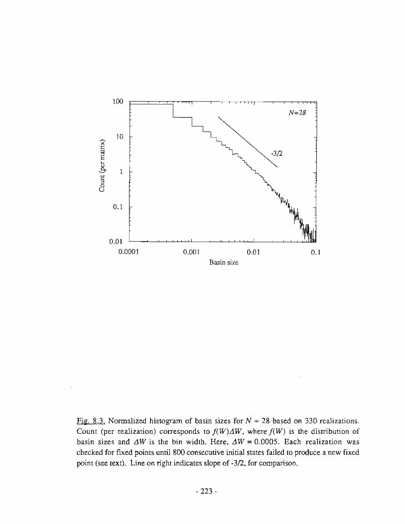
~
" 'C Ol E ~
8. ~
C " o
U
100
10
l
0.1
0.01
0.0001
N;28
0.001 0.01 0.1
Basin size
Fig. 8.3. Normalized histogram of basin sizes for N = 28 based on 330 realizations. Count (per realization) corresponds to j(W)Ll W. where j(W) is the distribution of basin sizes and LI W is the bin width. Here. LI W = 0.0005. Each realization was checked for fixed points unril 800 consecutive initial states failed to produce a new fixed point (see text). Line on right indicates slope of -3(2. for cornparison.
- 223-
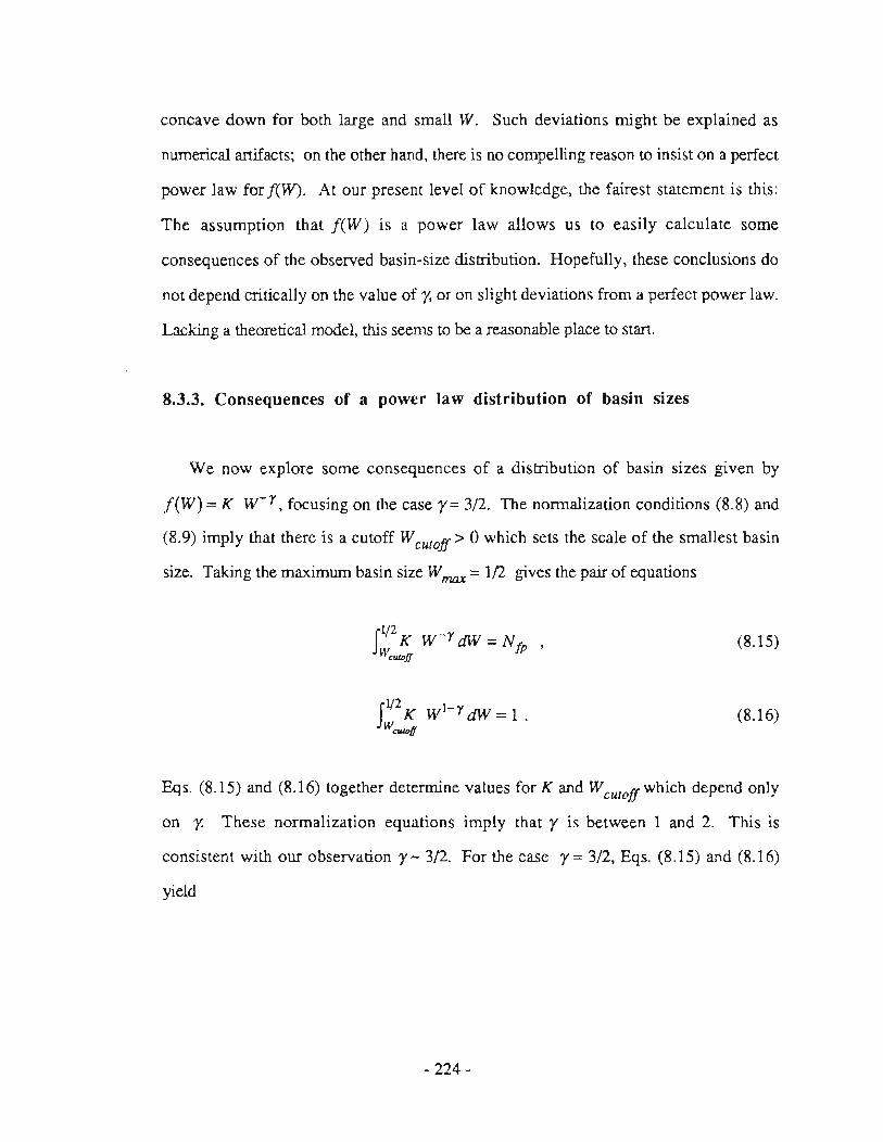
eoneave down for both large and smal! W. Sueh deviations might be explained as
numerical artifaets; on the other hand, there is no eompelling reason to insist on a perfeet
power law for f(W). At our present levelof knowledge, the fairest statement is this:
The assumption that f(W) is a power law allows us to easily calculate some
consequences of the observed basin-size distribution. Hopefully, these conclusions do
not depend critically on the value of y, or on slight deviations from a perfect power Jaw.
Lacking a theoretical model, this seems to be a reasonabJe pJace to start.
8,3.3. Consequences uf a power law distribution of basin sizes
We now expJore some consequences of a distribution of basin sizes given by
f(W) = K W-Y, focusing on the case y= 3/2. The normalization conditions (8.8) and
(8.9) impJy that there is a cutoff W cutoff > O which sets the scale of the smallest basin
size. Taking the maximum basin size W max = 1/2 gives the pair of equations
fl/2 K w-y dW - N w - lp
CWDff
(8.15)
(8.16)
Eqs. (8.15) and (8.16) together determine values for K and Wcutoffwhich depend onJy
on y. These normalization equations imply that y is between 1 and 2. This is
consistent with our observation y- 3/2. For the case y= 3/2, Eqs. (8.15) and (8.16)
yield
- 224-

.J2 K=---
2-4/Nfp [ Lim (K) = 1/.J2] N .... ~
(8.17)
Wc• ,off = 2N fp -2 ; [Lim (Wc• ,off ) = oJ N .... ~
. (8.18)
Equations (8.17) and (8.18) already lead to three rather surprising conclusions:
(i) The value of K depends very weakly on N, especially for larger values of N. That
means that the average (absolute) number of fixed points with basin size between W and
W+dW for any W> Wcu/Offis independent oJN.
(iO The cUloff of the power la w, W cutoff, tends to zero more slowly than the minimum
basin size W min as the size of the system N becomes large . Specifically,
W -0.398N h' l W -o.693N B I W h d . f b' f 11 eU/off - e w I e min - e . e ow cutoff' t e ens Ily o asms a s
rapidly to zero. Thus the smallest (typical) basin size is much larger than W min for large
N.
(iii) W cutoff is also lhe most common basin size, sinceJ(W) has its maximum at this
value. The value of W cutoff is different from the average basin size W ave' which is
l/Nfp by definition. Thus as the size of the system increases, the most common basin
size goes to zero faster than the average basin size.
Theoreticai values for W ave' Wcutoff' and W min are shown in Fig. 8.4(a) along
with numerical measurements of W cutoff for several values of N. Numerical values of
W cUloff are taken to be the maxim a of the histograms of basin sizes, as shown in
Fig. 8.4(b) for the case N = 22.
Higher moments of J(W) ean also be calculated. Using J(W) = K w-y with
y= 3/2 and values for K and Wculoff from (8.16) and (8.17), we find
- 225-

(a)
Fif;. 8.4. The small-basin cutoff Weurof! for the power law f(W) = K W-r with y = 3/2, as a function of system size N. From Eq. (8.18), Weuloff = 2N IP -2 = 2e-.398N. Also shown are the average basin size W ave = I/Nfp and minimum basin size W min = 2-N(N+I), beth of which are independent of the ferm ef f(W). Data (circ1es) are numerical values ef W eutof! for several values ef N, defmed as the maximum efthefiw), as shewn in (b) for the case N = 22.
- 226-

21- m N 2m _ 2mN y = t ) lp , m=0,1,2,3, ...
m Nfp2m-1 Nfp-2(2m-1) (8.19)
. 1 LIm [Yml = l' m = 1,2,3, ... N .... - (2m-1)2m-
(8.20)
Of particular interest is second moment Yz, which approaches the value 1/6 as the
system size (and thus the number of fixed points) becomes large, according to (8.20).
Numerical results of Gutfreund et al.[1988] for a system identical to (8.1), generalized
to include asymmetric connections, showed that Y2 tends to zero as the system size
increases for symmetric connections. The data of Gutfreund et al. were obtained using a
different technique from ours, one which tested only !Wo initial conditions per realization
and sampled an extremely large number of realizations. Repeating these measurements
using our probabilistic method also indicates that the numerical value of Y2 tends to zero
, not 1/6, as N becomes large. This disagreement shows that a strict -3/2 power law
does not provide a completely accurate description of j(W). In panicular, the -3/2
power law must exaggerate the number of large basins, leading to a finite second
moment.
8.4. DISTRIBUTIONS FOR OTHER MODELS
There is theoreticai and numerical evidence for universal it y in the way state space
breaks into clusters - basins of attraction, for example - in dynamical systems with many
attractors [Derrida and Ryvbjerg, 1986, 1987a, 1987b; Derrida, 1988b; Gutfreund et
al., 1988]. This section provides a brief summary of results for some of the systems
which show these universal propenies.
- 227-

8.4.1. Clusters of states in the SK model
Mezard et al.[1984a, 1984b] supplied a crucial piece of the spin glass puzzle by
describing the state space of the SK model in terms of a hierarchical or ultrametric
geometry. Ultrametricity gave deep physical insight into the meaning of the Parisi order
parameter q(x). and also provided a satisfying picture of the state space of a spin glass
as a hierarchy of valleys within valleys [Mezard et al., 1987; for a review of
ultrametricity, see: Rammal, 1986]. These papers [Mezard et al., 1984a; 1984b] also
presented an analytic form for the distribution of clusters of states3, with clusters
defined according to the mutual overlap q of states. We will present some of their
resuIts without providing detaiIs (see Mezard et al., 1987, Ch. IV, for a very readable
account).
Consider a division of the state space of the SK model into clusters, such that states
with overlap larger than q belong to the same cluster. The overlap between a pair of
states a and {3 is defined qa{3 = N-l l.i(S/,')(S!) with brackets denoting a
thermodynamic expectation value. Define W s to be the size of the srh cluster. When
averaged over realizations, the cluster sizes will form a continuous distribution j(W), which was given by Mezard et al. [1984a; 1984b l,
(8.21)
The quantity y in (8.21) depends on the choice of q used to set the cluster size and also
on physical parameters such as temperature and applied magnetic fieId. The gamma
3Throughout this section the term "states" will refer to equilibrium states, or states separated by energy barriers that become infinite in the thermodynamic limit. At T = O, equilibrium states of the SK model are equivalent to fixed points of the dynamical system (8.1).
- 228 -

functions in (8.21) normalize J(W) so that
f J(w)w dW = I. (8.22)
The derivation ofJ(W) takes into account the Boltzmann probability of a state being
present in counting the number of states in a cluster. Setting q to its maximum value,
which is qEA (the Edwards-Anderson order parameter) reduces the cluster size sueh that
each cluster comains just a single state (recaU: qEA == qaa is the equilibrium overlap af a
state with itself). For this ehoiee of q, the funetionJ(w) is just the average density of
states with Boltzmann weight W. That is, for q= qEA the weight W .. (y(q» of the
s/h state is given by
-ØF e ' (8.23)
where f3 = l/kT and F .. is the free energy of the s/h state.
It ean be shown that y(q) for q = qEA is given by the 1ength of the plateau of the
Parisi arder parameter q(x) [Mezard er al., 1984a, 1984b). A value for y( qEA) ean
be found using an approximation known as the PaT hypothesis [Vannimenus et al.,
1981], which assumes certain quantities to be independent af magnetic field and
temperature. In the limit T ..... O the PaT hypothesis gives
Limy(qEA) =.!.. r .... o 2 (8.24)
Inserting (8.24) imo (8.21) gives the folIowing encouraging result: For small elusters,
- 229-

j-(W-) - ~W--3/2 , W- l T O « , -t . n
(8.25)
Before celebrating the appearance of a -3/2 power law, we emphasize two points:
(i) Recall what we have found. j(W)d~V is the number of states with Boltzmann
weight between W and W +dW. It is not at all clear how this weight is related to the
basin size, although Fig. 8.1 may offer some clues.
(ii) We have considered the solution as T -t O because in this limit, the fixed points of
(8.1) correspond to thermodynamic equilibria of the SK model. However, another effect
of the T -t O limit is to heavily weighl the states with lowest free energy. Thus
j(W;T -t O) pertains only to the lowest energy states, nOl all equilibria. This explains
why the distribution i( W) has a divergence at W -t I : As T -t O the sum in the
denominator of (8.23) is dominated by a single term, the ground state for that realization.
When the state s in the numerator of (8.23) is the ground state, the numerator is nearly
equal to the denominator, so W gs - l. Note that the divergence inj(W) as W -t 1 IS
not present in the distribution of basin sizesfiW) which must vanish above W = 1/2.
Nevertheless, the form of (8.25) is tantaJizing. At present, however, we do not have any
satisfying way to relate this resuIt to the observed power law for the distribution of basin
slzes.
8.4.2. The Kauffman Model and the Random Map
Kauffman introduced a simple modelof genetic mutation and adaptation which shares
many features with spin glass models [Kauffman, 1969, 1984, 1990]. The model
consists of N sites, representing individual genes, each of which is characterized by a
binary state (O or 1) indicating one of two possibIe aJleles for that gene. Each site is
affected by exactly K sites, selecled al random from the N sites in the system. The
- 230-

response of a site to its K inputs is a random Boolean function which is chosen
independently for each site, and is flxed for all time (i.e. quenched) once chosen. The
dynanlics are deterministic and parallel, with each site folIowing its random truth table
(2K input states assigned randomly to a O or l output slate). Because the model is
detenninistic and has a discrete and fmile slate space, all attraetors must be periodic, with
periods ranging from l (fixed points) to 2N.
The distribution of basin sizes in the Kauffman model has been studied numerieally
as a funetion of K [Derrida and Flyvbjerg, 1986; see also Kauffman, 1990 for basin size
vs. energy plots similar to Fig. 8.3]. The numerical results of Derrida and Flyvbjerg
[1986] sug gest a surprising universality: moments of the distribution of basin sizes,
plotted one against another, agree extremely well with analytieal results relating the
moments of J(w), the distribution of weights in the SK model. Such agreement
indicates that certain statisticai propenies of multivalley state spaces are in sensitive to the
detaiIs of the underlying dynarnical system.
In the limit K __ 00, the Kauffman model is equivalent to a random mapping of an
N-dimensional binary space onto itself [Derrida and Flyvbjerg, 1987a, 1987bJ. (Note
that the limit K __ 00 ean be taken even for finite N, since the eonnection rule does not
restriet how many times a particular site may appear in a truth table.) In contrast to the
Kauffman model with general K, the random map model is mathematieally traetable, and
many of its statisticaI propenies are known analytically [Harris, 1960]. From these
results, Derrida and Flyvbjerg [1987a, 1987b] derived the following exaet expression for
the distribution of basin sizes in the random map model:
(8.26)
- 231 -

Note the similarity between fRM(W) and the distribution of weights i( W) for the SK
spin glass in Eq. (8.21). Of particular interest is the divergence at W = 1 comrnon to
both, but absent in the distribution of basin sizes for our system (8.1).
8.4.3. The l-D spin glass
The one dimensional (l-D) spin glass at zero temperature is another example of a
system with many attractors for which the distribution of basin sizes is known exactly
(the other being the random map). In this case, the result is that all the basins are the
same size, that is,flW) is given by Eq. (8.11) [Ettelaie and Moore, 1985; Derrida and
Oardner, 1986].
Derrida and Oardner [1986] analyzed the metastable states of a l-D chain of L Ising
spins with symmetric nearest neighbor coupling and free ends. The dynamics they
considered were single spin flip, with either random or deterIninistic order of updating.
Their results do not depend on the detaiIs of the distribution p( 1ij) of the random
connections, as long as it is symmetric ( p(1ij)=P(-Tij) ) and contains no delta
functions. They find that the typical number of metastable states in a realization of length
L is Nfp = 2LfJ and that the average number (over realizations) is N'};e = (4/,,)L [see
also: Li, 1981; Ettelaie and Moore, 1985]. That the average and typical number of ftxed
points in a realization are not equal is characteristic of short range models; for the infinite-
range SK model, NIP = N'};e.
It may seem surprising that the l-D spin glass has many metastable states, since it is
not frustrated in the sen se of Toulouse [1977] (see § 4.3.2). Indeed, for zero external
field - where the number of metastable states achieves its maximum [Derrida and
Gardner, 1986] - the l-D spin glas s is equivalent to a purely ferromagnetic chain by a
Mattis transformation [Mattis, 1976], albeit a ferromagnet with a distribution of
- 232-

ferromagnetic coupling strengths. How then, can such a system possess an exponential
number of metastable states? The answer is that single-spin-flip dynamics does not allow
kinks at weak bonds to unkink themselves. This point is illustrated by a simple example
with four spins and three ferromagnetic bonds, two strong ones on either side of a
relatively weak one.
For this configuration, no single spin flip will allow the weak bond in the middle to
become satisfied. The metastable state shown is also stable for parallel updating of spins.
On the other hand, an update rule which checks for energy reduction upon
simultaneously flipping pairs of spins will eliminate the metastable state shown. Moore
[1987] has discussed the computational efficiency of update rules which use multiple spin
flips to eliminate local energy minima. Finally, we note that recasting the l-D chain in
terms of analog state variables - by replacing Sgn[h] with ranh[j3h] in (8.1), for
instance - can also be used to reduce the number of metastable states. Continuing with
the simple four spin arrangement above, with the particular connection strengths ITd =
IT 341 = (3!2) IT 231, setting j3 < 1.44 will destabilize the metastable states, while the
ground states will remain stable for f3 > 0.48. This holds for sequential, parallel, or
continuous-time analog dynamies.
- 233 -

8.5. BASIN SIZES IN AN ANALOG SPIN GLASS
The last example in the previous seetion showed how reeasting a binary system into
its analog eounterpart ean dramatieally ehange the system's energy landseape. This idea
was also diseussed at length in Ch. 7. What effeet will using analog state variables have
on the basin strueture? We address this question for an analog version of the SK spin
glass,
j = 1, ... , N. (8.27)
where the states xj(l) now take on eontinuous values. As before, connection strengths
Tjj are symmetric (Tjj = Tj ) and gaussian distributed aecording to (8.2). In the limit
oflarge gain, f3 --* 00, (8.27) reduces to (8.1 ).
Figure 8.5 shows the distribution of basin sizes and energies for the analog spin glass
with N = 20 for two values of neuron gain, f3 = 4 and f3 = 20, averaged over 100
realizations. Basin-size counts and energies are based on binary states generated by
applying the Sgn funetion to an analog fixed point af ter convergence of (8.27). Initial
states were random corners of the unit hypercube, as before. The data in Fig. 8.5 show
that the reduction in the number of fixed points at lower gain (see § 7.2.1 for theory) is
strongly biased toward eliminating fixed points with small basin of attraction. For
example, we see from Fig. 8.5 that the average number of fixed points whose basins
occupy 0.1 of the state space (l05 initial states for N = 20) is essentially the same for f3
= 4 and f3 = 20, while the average number of fixed points with basins occupying 0.001
of the state space (103 initial states) is -50 times smaller at f3 = 4 than at f3 = 20. The
distribution of energies - calculated using (8.3) af ter applying the Sgn function to the
analog fixed point - also shows that lowering the gain shifts the distribution to lower
- 234-

(a)
N=20
10 ------ 1
~
" 'Ej
'"
, , - -, /3=20
E ....
1 8 E ::> o
U /3=4
0.1
0.01
0.001 0.01 0.1 Basin SIze
(b) N~20
3 . -.. '
'" " - :::::; '. " '5 ' .. :: : " . • 2 !: : E
], ::.,.; , :.~
c ~ :1 (3 I ~-.
::: ~ .. ::; :::' "
;' - "
O - --l -0.8 ·0.6 -004 -0.2 O
e
Fig. 8,5. Distribution af basin sizes and energies per site E. for the deterministic analog spin glass (defined in text) at two values af analog gain, f3 = 4 (solid line) and f3 = 20 (dashed line), for system size N = 20. 100 realizations were counted for each value af f3. The critical value af gain where fixed points first appear away from the origin (x = O) is f3 = 1/2, not f3 = 1, as it would be for the finite temperature spin glass. (a) Histogram af counts (per matrix) =!(W)LiW for a bin width LlW = 0.0025. Data show that lowering the gain greatly reduces the number af small basins, while leaving most af the big anes. (b) Histogram ( =!(E.)L1E. ) af fixed point energies per site E. = E/N. Bin width LiE. = 0.01. Lowering f3 reduces the number af fixed points and also shifts j(E.) to lower (more negative) energies.
- 235-

energies. This effect, however, is weak compared IO the shift in the basin-size
distribution. From these observations, we conclude that using analog state variables is
effective for selectively eliminating attractors with small basins, though not specifically
the most shallow attractoTS.
8.6. DISCUSSION AND OPEN PROBLEMS
We have found numericaIly that the distribUlionf(W) of basin sizes in the SK model
is approximately descibed by a power law with exponent - -3/2. Thus,[(W) appears
to be quite different from the distribution fRM(W) of basin sizes in the random map
model and different from the distribution l( W) of Boltzmann weights in the SK model.
So what has become of the universality of multi valley landscapes discussed by DeITida?
GUlfreund et al.[1988] have suggested that the general features of a multivalley
landscape depend on whether the number of attractors grows exponentially with system
size N. In the random map model for example, the average number of attractors (A) is
linear in N: (A) = N In 2/2 . This is different from the SK model, where the average
number of attractors is exponential in N. an the other hand, numerical data show that
the number of attractors for the fully asymmetric spin glas s does scale linearly with the
size of the system, and also that the distribution of basin sizes for the asymmetric spin
glass shares some common features withfRM(W) and i(w) [GUlfreund et al., 1988].
Perhaps basin structure, and the general structure of state space, can be divided into
universality cIas ses depending on whether the number of attractors does or does not
increase exponentially with N. At present, is not clear that such broad classes of
dynamicaI systems exist, or even by what phenomenological criteria such distinctions
ought to be made.
The resuIts presented in thi s chapter raise many new questions. Here are some:
- 236-

-- Will other techniques for measuring basin sizes yield the same results?
-- How do the the detail s of the dynarnics affect basin structure? For example, how is
state space shared between the fIXed points and the 2-cydes in a parallel version of (8.1)?
-- Why does a power law - or an approximate power law - appear? How is it related to
the ultrametric structure of state space?
-- How well do the results generalize to include (among other things) nongaussian
connection distributions, nonsymmetric connection, correlated connections, and
stochastic dynamies?
-- How can these resuIts be applied to neural networks, where control over basins of
attraction is of central importance? A first step in approaching such a question would be
to study the distributionf(W) in an associative memory as the number of stored pattems
p goes from p « N (the ferromagnetic limit), where presumably the basins for the
stored patterns are all the same size, to p »N, (the spin glass limit), where the
present resuIts should be recovered.
-- Is the weak correlarion between the energy or depth of a fixed point and the size of its
basin of attraction a general phenomenon? What abeut the correlarion between basin size
and the stability parameter /(, defined as the minimum of the distribution of local fields?
For the associative memory, numerical and analyticai evidence suggests that the
correlation between /(and basin size is strong [Forrest, 1988; Abbett, 1990).
- 237-

Chapter 9
CONCLUSIONS
In the introduction of this thesis, we discussed the idea that models of large nonlinear
systems ought IO be simple on a microscopic scale if one is to have any hope of
understanding their large-scale dynamicaI behavior. At that point, no mention was made
of how, given a physical system, one should go about separating wheat from chaff,
discarding the unimportant microscopic delluls and keeping the essentialones. Making
such distinctions a priori seems to be impossible; small changes often make big
differences, and vise versa. This distinction, and, more generaUy, how a dynamicai
system's microscopic features influence its large-scale behavior, is at the heart of the
controversy surrounding the whole neural network approach. One often hears that
describing a neuron as a binary threshold element is a ridiculous oversimplification. If
this is so, then why? Specifically, what global properties are lost, or even eroded, by
making such an approxirnation?
In this thesis, we have studied how properties of analog neural networks at the level
o/ the individunI neuron affect the large-seale dynamics of the network, and how thi s
effect is related to global network properties such as the spectrum of eigenvalues of the
connection matrix. The neuron properties we have considered are especially relevant to
designing fast, stable neural networks in electronic hardware. For example, an electronic
neuron (or a biological neuron for that matter) does not have an infinite switching speed,
and so, in principle, one must aeeount for any delay in describing the overall dynamies of
the network. Intuition teUs us that when the delay is extremely small (compared to some
characteristic time of the network), it ean probably be ignored. In thi s case, a simple
- 238-

model which assumes instantaneous response will suffice. But when is small no longer
small? At some point the chaff becomes wheat, and the delay must be accounted for.
The problem of delay-induced instability was discussed in detail in chapters 3 and 4. In
this example and throughout the thesis, we found that the gain of the neuron (i.e.
maximum slope of its transfer function) has a strong influence on the global dynamics of
the network. In several instances, the influence of neuron gain could be reduced to a
simple stability <,TIterion for insuring convergence of the dynamics to a fixed point.
From a practical point of view, the most important conclusion of this thesis is that
networks of analog neurons offer important computational advantages over networks of
binary (Ising) elements. Those advantages are: (1) SymmetricaIly connected analog
networks can be updated in parallel with guaranteed convergence to a fixed point. In
general, networks with binary neurons must be be updated sequentially to prevent
oscillation. Parallel updating is faster than sequential updating by a factor of O(N)
where N is the number of neurons in the network. (2) Lowering the gain of analog
neurons shows many of the beneficial effects of using temperature to escape local
minima. This was demonstrated numericalJy for associative memories in Ch. 5, and an
explanation for this surprising effect was given in Ch. 7. Specifically, it was shown in
Ch. 7 that lowering the neuron gain dramaticalJy reduces the number of local minima in
the network's energy landscape. (3) The analog networks we considered have
deterministic dynarnies, which means that they ean be built using standard analog VLSI
technology. Implementing a stochastic update rule in hardware is difficult because ofthe
need for lots of random numbers. Implementing a stochastic algorithm with parallel
dynamics in e!ectronics would be even more difficult, as it would require N independent
random numbers at each time step. Deterministic annealing could also be implemented
easily in analog VLSI by changing all neuron gains simultaneously via a single control
line.
- 239-

One might also be lead to speculate that the analog character of biological neurons -
that is, their well-known graded response - has similar computational significance, rather
than being an artifact of evolution.
Another significant idea which has emerged in this work is that certain analyticaI
techniques originally developed for Ising spin glasses, and later extended to treat binary
neural network models, can also be successfully adapted to the study of analog neural
networks. The analysis of storage capacity leading to the phase diagrams in Ch. 5 and
the analysis of the number of local minima for the analog spin glass and associative
memory in Ch. 7 are two places where techniques developed for discrete systems have
been adapted to the analog problem.
The systems we have considered were not arbitrarily chosen by any means. One
should not get the impression that relaxing some of the assumptions made will make the
problem only slightly more difficult. Usually, things get much harder. The most
restrictive assumption made throughout the thesis was that the coupling was symmetric.
Neural networks with asymmetric connections have vastly richer dynamics but are
correspondingly more difficult to approach analytically. The extension of the present
results to include asymmetric networks is the first and most obvious direction in
extending the present results. Be warned, this fust step is a big one. Another example:
The analysis of the multistep network in Ch. 6 does not generalize in any simple way to
allow weighted averages of previous time steps. It is unclear whether qualitatively new
dynamics would arise if different weights were allowed. One thing is certain: the present
analytical approach quickly runs aground when the assumption of equal weights is
relaxed.
Finally , we end with some interesting but unanswered questions:
Why is chaos so rare in finite-size networks? Can a "learning algorithm" be
developed to train a network to be chaotic?
- 240-

-- A related q uestion is how to train a network to possess higher dimensional attractors,
or chaotic attractors with a specific (noninteger) dimension. Measuring the dimension of
an attractor is straightforward, so there ought to be a way to develop a training algorithm
which yields an attractor of arbitrary dimension.
-- How can nonsigmoidal neuron transfer functions be used to advantage? One
example, the smooth staircase function, is discussed in Ch. 5. What about nonmonotonic
functions? Certainly from a dynamics point of view nonmonotonic neurons are more
interesting. But interesting is not what one wants in a neural network. Boring and
predictable make for robust computation.
-- What other sorts of problems, besides associative memory and a few ad hoc
optimization problems, can take advantage of the extensive feedback of Hopfield-type
networks? An answer to this question will determine whether this model is destined to
become a valuable technology or an academic curiosity.
- 241 -

Chapter 10
APPENDIX:
REPRINTS OF CHARGE-DENSITY W A VE PAPERS
Reprinted with pennission from the American Physical Society
- 242-

REFERENCES
Abbot!, L. F., (1990), Network l, 105.
Aguirregabiria, J. M., and J. R. Etxebarria, (1987), Phys. Lett. A 122, 241.
Aihara, K., T. Takabe, and M. Toyoda, (1990), Phys. Let!. A 144, 333.
Arnari, S., (1971), Proc. IEEE, 59, 35.
Amari, S., (1972), IEEE Trans. SMC-2, 643.
Amit, D. J., H. Gutfreund, and H. Sompolinsky, (1985a), Phys. Rev. A 32, 1007.
Arnit, D. J., H. Gutfreund, and H. Sompolinsky, (1985b), Phys. Rev. Lett. SS, 1530.
Arnit, D. J., H. Gutfreund, and H. Sompolinsky, (1987), Ann. Phys. NY 173, 30.
Arnit, D. J., (1989), Modeling Brain Function: The World of Arrractor Neural Networks, (Cambridge University Press, Cambridge).
an der Heiden, U., (1979), J. Math. Bio!. 8, 345.
an der Heiden, U., (1980), Analysis of Neural Networks, Vo!. 35 of Leerure Nores in
Biomathematics (Springer, New York) .
Anderson, D. Z., (1988), Ed., Neural Information Processing Systems, Denver CO,
1987 (AlP, New York).
Ashcroft, N. W., and N. D. Merrllin, (1976), Solid State Physics, (Saunders College,
Philadelphia).
Babcock, K. L., and R. M. Westervelt, (l986a), Physica 230, 464.
Babcock, K. L., and R. M. Westervelt, (l986b), Physica 280, 305.
Barlow, R. B., and A. 1. Fraioli, (1978), J. Gen. Physio!., 71, 699.
- 252·

Basharan, G., Y. Fu and P. W. Anderson, (1986), J. Stat. Phys. 45, l.
Baudet, G. M., (1978), J. Assoc. Comp. Mach. 25, 226.
Bauer, M., and W. Martienssen, (1989), Europhys. Lett. 10,427.
Bellman, R, and K. L. Cooke, (1963), Differential·Difference Equations (Academic Press, New York).
Berge, P., Y. Pomeau, and C. Vidal, (1984), Order wirhin Chaos, (Hermann, Paris).
Bilbro G., R Mann, T. Miller, W. Snyder, D. Van den Bout, and M. White, (1989), in Advances in Neurallnformation Processing, Denver CO 1988, edited by D. S. Touretzky (Morgan Kaufmann, San Mateo), p. 568.
Bilbro G., and W. Snyder, (1989), in Advances in Neurallnformation Processing, Denver CO 1988, edited by D. S. Touretzky, (Morgan Kaufmann, San Mateo), p.594.
Binder, K., and A. P. Young, (1986), Rev. Mod. Phys. 58,801.
Blake, A., and A. Zisserman, (1987)'yisual Reconstruction (MIT Press, Cambridge, MA).
Blume, M., (1966), Phys. Rev. 141,517.
Bray, A. J., and M. A. Moore, (1979), J. Phys. C 12, L441.
Bray, A. J., and M. A. Moore, (1980), J. Phys. C B, L469.
Bray, A. J., and M. A. Moore, ( 1981), J. Phys. C 14, 1313.
BroU!, R, (1959), Phys. Rev. 115, 824.
BroU!, R., and H. Thomas, (1967), Physics 3, 317.
Bruce, A. D., E. J. Gardner, and D. J. Wallace, (1987), J. Phys. A 20, 2909.
- 253-

Buhmann, J., and K. Schulten, (1987), Europhys. Lett. 4,1205.
Burgess, N., and M. A. Moore, (1989), J. Phys. A 22, 4599.
Cabasino, S., E. Marinari, P. Paolucci, and G. Paris i, (1988), J. Phys. A 21, 4201.
Capel, W., (1966), Physica 32, 966.
Carpenter, G. A., M. A. Cohen, and S. Grossberg, (1987), Science 235, 1226.
Chaffee, N., (1971), J. Math. Anal. and Appl. 35, 312.
Choi, M. Y., and B. A. Huberman, (1983a), Phys. Rev. B 28, 2547.
Choi , M. Y., and B. A. Huberman, (1983b), Phys. Rev. B 31, 2862.
Chowdhury, D. (1986), Spin Glasses and Other Frustrated Systems , (Princeton
U niversity Press, Princeton, NJ).
Cohen, M. A., and S. Grossberg, (1983), lliEE Trans. SMC·13, 815.
Coleman, B. D., and G.H. Renninger, (1975), J. Theor. Bio!. 51, 243.
Coleman, B. D., and G.H. Renninger, (1976), SlAM J. App!. Math. 31, 111.
Coleman, B. D., and G.H. Renninger, (1978), Math. Biosc. 38, 123.
Coolen, A. C. C., and C. C. A. M. Gielen, (1988), Europhys. Let!. 7, 281.
Cragg, B. G., and H. N. V. Temperley, (1954), E1ectroenceph. Clin. Neuro. 6, 85.
Crisanti, A., and H. Sompolinsky, (1987), Phys. Rev. A 36, 4922.
Crisanti, A., and H. Sompolinsky, (1988), Phys. Rev. A 37, 4865.
De Dominicis, C. ,M. Gabay, T. Garel, and H. Orland, (1980), J. Physique 41, 923.
Dehaene, S., J. P. Changeux, and J. P. Nadal, (1987), Proe. Nat. Acad. Sci. USA 84,
2727.
·254·

Denker, J. S., (1986a), Physica 22D, 216.
Denker, J. S., (I 986b), Ed., Neural Networks for Computing, ATP Conf. Proc. 151 (Ameriean lnstitute of Physics, New York).
Denker, J. S., (1986c), in Neural Networks for Computing, edited by J. S. Denker,
AlP Conf. Proc. 151 (Ameriean Tnstitute of Physics, New York)., p. 121.
Derrida, B., (1988a), J. Phys. A 20, L721.
Derrida, B., (l988b), in Nonlinear Evolution and Chaotic Pl!eMmena, Proc. of N A TO Adv. Study Workshop - Noto, Sicily, ltaly, June 1987. (Plenum, NY), p. 213.
Derrida, B., and H. Flyvbjerg, (1986), J. Phys. A 19, LID03.
Derrida, B., and H. Flyvbjerg, (1987a), J. Physique (Paris) 48, 971.
Derrida, B., and H. Flyvbjerg, (1987b), J. Phys. A 20,5273.
Derrida, B., and E. Gardner, (1986), J. Physique (Paris) 47, 959.
Diederich, S. , and M. Opper, (1987), Phys. Rev. Lett. 58, 949.
Domany, E., W. Kinzel, and R. Meir, (1989), J. Phys. A 22, 2081.
Dowling, J. E., (J 987), The retina: An approachable part ofthe brain (Harvard Univ.
Press, Cambridge, MA).
Durbin R., and D. Willshaw, (1987), Nature 326, 689.
Edwards, S. F., and R. C. Jones, (1976), J. Phys. A 9, 1595.
Ettelaie, R., and M. A. Moore, (1985), J. Physique Lelt. 46, L893.
Farmer, J. D., (1982), Physica 4D, 366.
Fiseher, K. H., (1976), Solid State Commun., 18, 1515.
- 255-

Fleisher, M., (1988), in Neural Information Processing Systems, Denver CO, 1987, edited by D. Z. Anderson (AlP, New York), p. 278.
Fontanari, J. F., and R. Koberle, (1988a), J. Phys. (France) 49,13.
Fontanari, J. F., and R. Koberle, (l988b), J. Phys. A 21, L259.
Fontanari, J. F., and R. Koberle, (l988c), J. Phys. A 21, L667.
Forrest, B. M., (1988), J. Phys. A 21, 245.
Fradkin, E., B. A. Huberman, and S. H. Shenker, (1978), Phys. Rev. B18, 4789.
Frumkin, A., and E. Moses, (1986), Phys. Rev. A 34, 714.
Fu, Y., and P. W. Anderson, (1986), J. Phys A 19, 1605.
Fukai, T., (1990), J. Phys. A 23, 249.
Gardner, E. J., (1986), J. Phys. A 19, Ll047.
Gardner, E. 1., (1988), J. Phys. A 21, 257.
Geman, S., (1980), Ann. Prob. 8, 252.
Glass, L. and M. C. Mackey, (1988), From Cloeles to Chaos - The Rhythms of Life, (Princeton University Press).
Golden, R. M., (1986), J. Math. Psych. 30, 73.
Goles, E., and G. Y. Vichniac, (1986), in Neural Necworksfor Computing, edited by J. S. Denker, AlP Conf. Proc. 151 (American Institute of Physics, New York),
p .165.
Goles-Chacc, E., F. Fogelman-Soulie and D. Pellegrin, (1985), Disc. Appl. Math. 12,
26l.
Grinstein, G., C. Jayaprakash, and Y. He, (1985), Phys. Rev. Lett. 55, 2527.
Grossberg, S., (1970), Stud. Appl. Math. 44, 135.
- 256-

Grossberg, S., (1988), NeuraJ Networks l, 17.
Guckenheimer, J., and P. Holmes, (1983), Nonlinear Oscillations, Dynamieal Systems and Bifureations ofVeetor Fieids (Springer, NY).
Gutfreund, H., and M. Mezard, (1988), Phys. Rev. Lett. 61, 235.
Gutfreund, H., J. D. Reger, and A. P. Young, (1988), J. Phys. A, 21, 2775.
Guyon, I., L. Personnaz, J. P. Nadal, and G. Dreyfus, (1988), Phys. Rev. A 38,
6365.
Hadeler, K. P. , and 1. Tomiuk, (1977) , Arch. Rat. Mech. Anal. 65,87.
Hale, J. K., and N. Sternberg, (1988), J. Comp. Phys. 77, 221.
Harris, B., (1960), Ann. Math. Stat. 31, 1045.
Hebb, D. O., (1949) , The Organization of Behavior (Wiley, New York).
Hentschel, H. G. E., and A. Fine, (1989), Phys. Rev. A 40, 3983.
Hertz, J. A., G. Grinstein, and S. A. Solla, (1987) in Proc. Heidelberg Colloquium on Glassy Dynamics, Vol. 275 of Leeture Nores in Physics, edited by L. J. van Hemmen and I. Morgenstem, (Springer, Berlin).
Herz, A., B. Sulzer, R. Kiihn, and J. L. van Hemmen, (1988), Europhys. Let!. 7, 663.
Hirsch, M. W., (1987), Convergence in Neural Nets, in Proc. of rhe IEEE Conf. on Neural Networks, San Diego, CA, edited by M. Caudill and C. Butler, (IEEE, New York).
Hirsch, M. W., (1989) , NeuraJ Networks 2, 331.
Hopfieid, J. J., (1982), Proc. Nat. Acad. Sci. USA 79, 2554.
Hopfieid, J. J., (1984), Proc. Nat. Acad. Sci. USA 81, 3008.
Hopfieid, J. J., and D. W. Tank, (1985), Biol. Cybem. 52, 141.
- 257 -
Hopfieid, J. J., and D. W. Tank, (1986), Science 233, 625.
Jeffrey, W., and R. Rosner, (1986a), Astr. J. 310, 473.
Jeffrey, W., and R. Rosner, (1986b), in Neural Networks for Compuring, edited by J. S. Denker, AIP Conf. Proc. 151 (American Institute of Physics, New York), p.241.
Kanter, 1., (1989), Phys. Rev. A 40, 2611.
Kanter, 1., (1990), Europhys. Lett. 11, 397.
Kanter, I., and H. Sompolinsky, (1987), Phys. Rev. A 35, 380.
Kauffman, S. A. (1969), J. Theor. Bio!. 22,437.
Kauffman, S. A. (1984), Physica IOD, 145.
Kauffman, S. A. (1990), Origins ofOrder: SelfOrganization in Evolution, (Oxford University Press, Oxford).
Keeler, J. D., (1986), in Neural Networks for Compuring, edited by J. S. Denker, AlP Conf. PrOC. 151 (American Institute of Physics, New York), pg. 259.
KepIer, T. B., (1989), Model Neural Networks, Ph. D. dissenation, Brandeis University.
KepIer, T. B., and L. F. Abbott, (1988), J. Physique 49, 1657.
KepIer, T. B., S. Datl. R. B. Meyer. and L. F. Abbou, (1989), Chaos in a neural
network circuit, Brandies University preprint BRX-2.65.
Kerszberg, M., and A. Zippelius, (1989), Synchronization in Neural Assemblies, preprint .
Kirkpatrick, S., C. D. Gelatt, Jr. and M. P. Vecchi, (1983), Science 220,671.
Kirkpatrick, S., D. Sherrington, (1978), Phys. Rev. B 17,4384.
- 258-

Kleinfeld, D., (1986), Proc. Nat. Acad. Sci. USA 83, 9469.
Koch, c., J. Marroquin, and A. Yuille, (1986), Proc. Nat. Acad. Sci. USA 83, 4263.
Kolmanovskii, V.B., and V.R. Nosov, (1986), Stability of Funcrional Differential Equations (Academic Press, New York).
Krauth, W., M. Mezard, and J. P. Nadal, (1988), Complex Systems 2, 387.
Kiihn, R., J. L. van Remmen, and U. Riedel, (1989), J. Phys. A, 22, 3123.
Kiirten, K. E., (1988), Phys. Let!. 129A, 157.
Kiirten, K. E., and J. W. Clark, (1986), Phys. Len. 114A, 413.
Li, T., (1981), Phys. Rev. B 24, 6579.
Ling, D. D., D. R. Bowman, and K. Levin, (1983), Phys. Rev. B 28, 262.
Lippmann, R. P., (1987), IEEE ASSP, April issue, 4.
Linie, W. A., (1974), Math. Biosci. 19, 101.
Linie, W. A., and G. L. Shaw, (1978), Math. Biosci. 39, 281.
Lynch, G., (1986), Synapses, Circuits, and the Beginnings of Memory, (MIT Press, Cambridge, MA).
Mackey, M. c., and U. an der Heiden, (1984), J. Math. Biology, 19, 221.
Mackey, M. c., and L. Glass, (1977), Science 197,287.
Maddox, J., (1987), Modelling for its own sake, Nature 328,571.
Marcus, C. M., and R. M.Westervelt, (1988), in Neuralinformation Processing Systems, Denver CO, 1987, edited by D. Z. Anderson, (AlP, New York), p. 524.
Marcus, C. M., and R. M.Westervelt, (1989a), Phys. Rev. A 39, 347.
- 259-
Marcus, C M., and R. M.Weslervelt, (1989b), in Advances in NeuraiInformation Processing, Denver CO 1988, ediled by D. S. Touretzky (Morgan Kaufmann, San Mateo), p. 568.
Marcus, CM., and R. M. Westervelt, (1989c), Phys. Rev. A 40, 501.
Marcus, C M., and R. M.Westervelt, (1990), to appearin Phys. Rev. A.
Marcus, C M. , F. R. Waugh, and R. M.Westervelt, (1990), Phys. Rev. A, 41, 3355.
Mattis, D. C, (1976), Phys. Lel!. 56A, 421.
May, R. M., (1974), Stability and Cornplexity in Model Ecosystems, 2nd Ed. (Princeton University Press, New Jersey).
May, R. M., (1976), Nature 261, 459.
McCulJoch, W., and W. Pilts, (1943), BulJ. Math. Biophys. 5, 115. Reprinted in Brain Theory, Reprint Volurne, Advanced Series in Neuroscience, Vol . 1,ed. by G. L. Shaw and G. Palm (Wor1d Scientific, Singapore, 1988).
Mead, Carver A., (1989), Analog VLSI and Neural Systems (Addison-Wesley, Reading, MA).
Meir, R., and E. Domany, (1987), Phys. Rev. Lel!. 59, 359.
Meir, R., and E. Domany, (1988), Phys. Rev. A 37, 608.
Meunier, C, D. Hansel and A. Verga, (1989), J. SIa!. Phys. 55, 859.
Mezard, M., G. Parisi, N. Sourlas, G. Tou1ouse, and M. A. Virasoro, (1984a), Phys. Rev. Len. 52, 1156.
Mezard, M., G. Parisi, N. Sourlas, G. Toulouse, and M. A. Virasoro, (1984b), J. Physique (Paris) 45, 843.
Mezard, M., G. Parisi, and M. A. Virasoro, (1987), Spin Glass Theory and Beyond, (W orld Scientific, Singapore).
- 260-

Moore, M. A., (1987), Phys. Rev. Lett. 58, 1703.
Mukherjee, A., (1985), Introduction to nMOS and CMOS VLSI System Design, (Prentice Hall, New Jersey).
Nemoto, K., and H. Takayama, (1985), J. Phys. C 18, L529.
Nishimori, H., T. Nakamura, and M. Shiino, (1990) Phys. Rev. A 41, 3346.
Ortega, J. M., and W. C. Rheinboldt, (1970),Jterative solution of nonlinear equations in several variables, (Academic Press, NY).
Opper, M., J. Kleinz, and W. Kinzel, (1989), J. Phys. A 22, L407.
Parga, N., (1987), J. Physique (Paris) 48, 499.
Parisi, G., (1986), J. Phys. A 19, L675.
Peretto, P., (1984), Bio!. Cybem. 50, 51.
Personnaz, L., I. Guyon, and G. Dreyfus, (1985), J. Phys. Lett. (Paris) 46, L359.
Rammal, R. G. Toulouse, and M. A. Viarsoro, (1986), Rev. Mod. Phys. 58, 765.
Ratliff, F., (1965), Mach Bands: Quantitative Studies on Neural Networks in the Retina, (Holden-Day, San Francisco).
Ratliff, F., (1974), Ed., Studies on Exitation and Inhibition in the Rerina, (RockefelIer University Press, New York).
Reger, J. D., and K. Binder, (1985), Z. Phys. B, 60, 137.
Reger, J. D., K. Binder, and W. Kinzel, (1984), Phys. Rev. B 30, 4028.
RenaIs, S., and R. Rohwer, (1990), J. Stat. Phys. 58, 825.
Riedel, U., R. Kiihn, and J. L. van Hemmen, (1988), Phys. Rev. A 38, 1105.
- 261 -

Rumelhan, D. E., J. L. McClelland, and the PDP Research Group, (1986), Parallel Distributed Processing, Explorations in the Microstrueture ofCognition, Voll and 2 (MlT Press, Cambridge, MA).
Shaw, G. L., and G. Palm, Eds., (1988), Brain Theory, Reprint Volurne, Advanced Series in Neuroscience, Vol. l,(World Scientific, Singapore, 1988).
Sherrington, D. and S. Kirkpatrick, (1975), Phys. Rev. Let!. 35,1792.
Shinomoto, S., (1986), Prog. Theor. Phys. 75, 1313.
Silverstein, J. W., (1985), Ann. Prob. 13, 1364.
Sommers, H. J., A. Crisanti, H. Sompolinsky, and Y. Stein, (1988), Phys. Rev. Let!. 60, 1895.
Sompolinsky, H., (1986), Phys. Rev. A 34, 2571.
Sompolinsky, H., (1988), Physics Today 41, No. 12,70.
Sompolinsky, H., A. Crisanti, and H. J. Sommers, (1988), Phys. Rev. Lelt. 61, 259.
Sompolinsky, H., and L Kanter, (1986), Phys. Rev. Lelt. 57, 2861.
Soukoulis, C. M., K. Levin, and G. S. Grest, (1982), Phys. Rev. Lelt. 48, 1756.
Soukoulis, C. M., K. Levin, and G. S. Grest, (1983), Phys. Rev. B 28, 1495.
Spitzner, P., and W. Kinzel, (1989), Z. Phys. B 77, 511.
Sze, S. M., (1981), Physics of Semiconductor Devices, 2e, (John Wiley, New York).
Tanaka, F. and S. F. Edwards, (1980), J. Phys. F IO, 2769.
Thouless, D. J., P. W. Anderson, and R. G. Palmer, (1977), Phil. Mag. 35, 593.
Toulouse, G., (1977), Commun. Phys. 2, 115.
Toulouse, G., (1989), J. Phys. A 22, 1959.
- 262-

Treves, A., and D. J. Amit, (1988), J. Phys. A 21, 3155.
van Hemmen, L. J., (1987), Phys. Rev. A 36, 1959.
van Hemmen, L. J., and I. Morgenstern, (1987), Eds., Proc. Heidelberg Colloqllillm on Glassy Dynamics, Vo!. 275 of Lecture Notes in Physics (Springer, Berlin).
Vannimenus, J., G. Toulouse, and G. Parisi, (1981), J. Physique (Paris) 42, 565.
Wannier, G. M., (1950), Phys. Rev. 79, 357.
Waugh, F. R., C. M. Marcus, and R. M. Westervelt, (1990), Phys. Rev. Lett. 64, 1986.
Weinitschke, H. J., (1964), Num. Math. 6, 395.
Wigner, E. P., (1958), Ann. Math. 67, 325.
Wyatt, Jr., J. L., and D. L. Stanley, (1988), in Neurallnjormation Processing Systems, Denver CO, 1987, edited by D. Z. Anderson, (AlP, New York), p. 860.
Yedidia, J. S., (1989), J. Phys.A 22, 2265.
Yuille, A., (1989), Bio!. Cybern. 61, 115.
- 263-

VOLUMEn!. NUMBER20 PHYSICAL REVIEW LETTERS 14 NOVEMBER 1988
Simple Model of CoUec:tite TraDSpOrt witb Pbase Slippage
S. H. Strogau:. (a) C. M. Marcus. and R. M. Westcrvcit Di"i$joll o/ Applied ScieflCe$ ønd INpdrlfMlIl af Physia. HarvtJrd UllilJersily.
Camim'dp. Mll$$øc/uuel1$ 02 J 38
R. E. MiroUo D~pt1rlm~lI' of Malhnnalia. Bro...,,, UIli~r$jIY. p,.avid~ffa. Rhode Island 02911
(Rcc:civcd 29 April 1988)
Wc present 3. mean-6c1d analysis a( a many-body dynunical system whicb models cbarae-density· wave transport in the prescnce af random pinning impuritics. Pbue slip betwc:en charse-density-wavc domains is modeled by a coupiing term that is periodie in the phase differenca. When driven by an Clternal fieid. the system exhibits a first~rder dcpinnina transition. hysteresis. and switching betwc:en PIDoed and slidin. stales" and il delayed OAset af slidine near tbrcsbold.
PACS numbtn: 71.45.Lr. 03.20.h OS.4S.+b. 72.IS.Nj
Collective transpon in c:oupled dyn am icai systems is a topic of considerable cum:nt interest. I An experimcntal example is thc nonlincar conduction seen in chargedensity-wave (CDW) samples. 2.3 When a sufficiently strong dc elcctric 6eld is appJicd to a sample with astatic CDW. the CDW dcpins from impurities in tbe lattice and begins to slide and carry current. Classical models of CDW transport'-IO assume thai the dynamics are dominaled by competition betweeD tht internaJ elasticity "af the CDW and the locaJ potentials of randomly spaced impurilies.
These models of CDW transport do not account for e,;,perimentaUy obscrvcd hysteresis. switching, and de.,; layod conduction in "switching samples:>!J-U CDW inertia. I' cumnt DOiK:. " and avalanche dtpinning It bave been proposed to account for switching. More rcccntly, switching aod hysteresis have been ascribed to pbase slippage in tbt CDW. 11·13 A pbysical model for a CDW in a switching sample is a collection of domains. each with a weH~c6ned phasc. separatcd by regions where the amplitude of the COW is weak. J2. J' Phase slip caD oecur easily in these connecting regions. A rigorous tbeory of CDW transpon for this case is very difficull, allbough a detaiJed anaJysis of a pbenomeoologica1 mod· el with a few degrees of frcedom bas beeD prcscnted. " It is also uncertain whicb of the ob$Crved complex pbenomena are intrinsic and which are properties of panicular samples ar experiment&1 trcatrnents.
]n tbis Letter we present a simple modelof coUective transpon which is applicable lO CDW transport in switching samples. Tbe model consislS af many pbases whicb represent tbe states of CDW domain5., and phase slip due to amplitude coUapscJS is modeJed by a wcakcouplioø term periodic iD. the phasc difi'erenccs. This is a simple moditication of a w~lI-uDdenlOOd model'" witb clastic coupliD.g and no pbue slip. AI we will show, thc pcriodic coupling gives rise to switcbiol, bysteresis, and delayed cooduction. OUf approacb is to analyzc l simple
model wbich may have sorne generalily, rather than to mate a dctailed pbenomenological treatment specific to charge-density waves.
Tbe Hamiltonian is
(la)
and we assume uro temperature and relaxationaJ dynamica with a driving field
. aH Oj--ae;+Eo. j-I .... ,N. (Ib)
The Sj represent the phases af weakJy coupled domaios. u In otber models,'·1 8j rcprexnt (he phase distortion of tbe CDW at the }th pinning site. In Eq. ()), J is the coupling strength, b is the pinning strength, ø j is a pinning phase randomly distributed an [- K,Jfl, and Eo is an electric ficld applicd along lhc CDW wave vector. Tbe coupling tcrm favors pbase coberencc. whereas tbc random fieids try to pin eacb Bj at a j o For weakly couplcd domains. tbe ratio K - J I b is small. The infiDite-raoge coupling in Eq. (t) ootTCSponds to tbc meao-6eld approximation. a1so used ror prcvious worL""'"
Tbe model (I) is closely related to tbe system studied by Fisher. 6 Tbe difference is that in the Hamiltonian Eq. Oa) we bave assumcd aperiodie coup1inS I -cos(8j
-Oj) rather than aquadr'lie couplin, t (O, -8j )'. Tbe periodie coupling in Eq. Oal aUow> for phasc-,Iip proc:esses,.1I and corresponds pbysicaUy to tbe effecu of CDW defccu 1.1' Dr amplitude coUapse 11.15 between cobemll ",gioQJ of Ihe CDW. In particular, Ih< model is appropriale in CDW ')'Items with Itronl pinom, centers tbat favor tbe formation Df wealdy coupled domaiDs. 12,20 Wc bave made the simplifying asrumption thaI Ih. araumenl ol Ihe periodic couplin, is Ih< pbue
2380 C 1988 Tbe American Pbysical Sociely
·243 -

VOLUME 61. NUMBER 20 PHYSICAL REVIEW LETTER S 14 NOVEMBER 1988
diJl'erence Bj - 9J rather tban a more generaJ multiple I.(S/ -9,), wbe ..... toets tbe amouot of poW'izatioa tbal can be built up befare ph.ue slip occurs. Additional mctasu.blc states IO witb di.ft'erent polarizations cau emt below tht depionms threshold for A,fIII! I; thcsc are not praent in OUf model.
Wc fint coDsider tbt statie configuration of tht system when Eo-O. Tbc pbasc cobcKncc of tht equilibrium conftgurations depeDds OD the normaJizcd coupling strcngtb K, For instante, in tbt absence of coupling (K-O), tht 8, are pinncd at a j aod are complctcly in· cohcrenl, whercas for K - GD, tbeR is perfect. cohcrcnce (8/-Ø, for all i,j). To charactcrizc tht traDsition from incohcrencc to coherence. wc defioe a complex order pa· rameter
,./' - N - , 1;, exp(;9,) ,
whcre r measurcs tht cohcreDce and , is tbt averagc ph ....
Wc now show anaJytically that lbere is a first-order transition in tbc model from the incobcrent state (r-O) to thc coherent state C,:It:: I) at K -2, when tbe domains are stroagly coupled. This uro--6eld transition is an artitaet of mcaa-tield tbeory, but a relatcd hystcrc:tic transitioD occun for Donzero Eo in the physically relevant weak-c:oupling regime, as discu.ssed below. Tbe strategy af tbe analysis is to derivc a self-consistent equation for r, by U$e of tbe faet tbat , detcrmines tbe equilibrium pbases .9J and is in turn determinc:d by them.
Equilibria of H satisfy aH las, -o, i.e .•
sio(a,-9,>+ Z ~Sio(9/-9,)-0. Rewriting tbe sum in tenns of the order parameter yields
sin(aJ - 9j )+K,sin(;:- 9j ) -O .
We ma)' set .-0 becausc theR is DO absolute phas.e reference. This choke removcs tbe rotational degeneracy. Solvin, Eq. (2) for 9, yields
(3)
Combinin, Eq. (3) witb r-N-'!.jexp(;9j ) and lettiog N - 00, wc obtain tbe self-consistency relation for r.
r-..LI· Kr+cosa da (4) 21r -. (I+2K'C0S4+X 2,l)l f2 .
For each K, tbe nlues af , that satisfy Eq. (4) may be found as rollo .... (Fig. )(a)1. Le, u -Kr and let /(u) dcnote the integral in Eq. (4), wbich may be expressc:d euetly as an eUiptic integral. 21 Bccause f(u) and u I K are betb equal to " tbe intersec:tions of f(u) and tbe line &ol I K yield solutioDJ for tbe coberenee " given tbe nor· malizcd coupling Slrenglb K (Fig. I (all.
Figure I (b) shoWI tbe fi.nt~rder transition betwccn incoberent and coberent states. lbe iDcobeunl slale
- 244-
ulK
r'Oj I(u)
05i
0.0 ;?l ~~ ___ ( a_I I bl
O 2 u K
FIG. I. (a) Solid lines indicate the Integral /(11) ploued (rom Eq. (4) topther with the line ulK (see tut>. Equilibrium solutions for,. oocur whcre /(11) inu:rsccts che line u/ K. For the value af K shoWl!, threc solutions exist (61Jcd c;:irclcs). Oashed lines show ul K for the critical values K -K~ and K-2. (b) Plot of Ihe cnct equilibrium solutions (or ,. vs K: solid lines. locally stable equilibria: brolc.en lines, unstable equilibria.
, -O always 50Ives Eq (4), An unstable second brancb of the solutions bifurcates from r -o at K - 2, with r - (2 - K) '}2 as cao bo seen from Eq. (4J and the .. ries expaosioo /(u)-u/2+u'/16+0(u'), valid for u < I. We have also plOvenll that ,-0 is locally stable for K < 2 and u .. table for K> 2. A hJeally stable tbi.u brancb af solutions. with ':11:::' I, · is creatcd when II I K interJeCU /(u) taogeotiaUy (Fig. l <all al K -K, .. 1.489. Note that for K between K( and 2, tbe system is bislable. Wc empbasize tbat thi! first~rder transition is a consequencc of tbe cosine coupling in Eq. Oa) and would not bc SC(:D ir a quadratic coupling were assumed.
Wc tum now from statics to dynamics. In the presenee af a driving fieid. tbe equations of motion from Eq. (Ib)"",
dS,/dl -E +Krsin(, - 9,) +sin(aj - 9J ) . (5)
By lelliog E-EoIb lOd time l-bl. ",e have ICt b-l witbout lou of generality; as before, X -J/b. Tbe lCCOod term an tbe tigbt-hand side of Eq. (S) il the collective torque exertod on Bj by aU other phases. For E -O and small K, the pbase coherence , -O and tberefore tbe collcctive torque is uro. If r becomes nonuro, tbe collective torque provides a positive feedback wbicb tries to incrcasc r runber by illigning eatb 9, witb tbe average pbasc.. Tbe physical conscquenccs of tbi.s proccss are hystercsls and delaycd conduction, as discw.sc:d bclow. In our model hystercsls and switching result rrom the transition to coberencc af a randomly pinncd state. locohcrencc of tbe piaoed state occun naturaU)' for a larae numbcr of random pinoing phases aj; systems as small as tbrce phases show hysteresis and switching, but ooly wbeo tbe a, are CbOSCD evenly spaccd on (-X,.Ir). lbus in our modelibese pbenomena are associatcd witb many degrccs of frccdom.
2381

VOLUME61, NUMBER20 PHYSICAL REVIEW LETTERS 14 NOVEMBER 1988
Figu", 2 plou the ",gian. af stability af the pinned aDd slidiDg CDW sta .... The piDoed state (dS/dI-O) in tbis model ca.n be analyticaUy sbown to be iDcobereot (r -O). Using variationaJ stability anaJysiJ abou. 'be pinned statc. wc have proven 21 tbat tbis state becomes unstable above tho dopinnin, thrcshold fiold E T - Cl - K 2/ 4) [/1 wben K < 2. as shown in Fig. 2. For strong coupJing. K> 2 whcre tbt model is not physically rolovant, ET -O and tho CDW slides (d.ldl > O) for aDY fieids E> O. This is an anifact of mun-6cld tbeory which al50 occurs in modcls64 witb elastic couphng. Numerical solutions of Eq. (S) show thai tbt: slidins state is always cohcrent (r> O), Tbc slidiog stale be· cama pinned and incobcrcnt beJow a separate pinning tbreshold E p shown as tht dasbed line in Fig. 2. whicb was calculated numerically (rom tbt initial coodition r-l. This boundary extends (rom tht critical value K~ (ound analytically for E -O, also shown in Fig. 1. The solid and dasbcd lines in Fig. 2 bound a hystcretic region wh.ere botb pinncd and slidiog solutions are stable; tbe final state reacbed depcods on tbe initial condilioos. The physicaUy relevant wcak-coupling region of Fig. 2 is for K < Kr, where ET and E, are nonum.
The model predicts bystercsis and switching between pinncd and sliding states as ilJustrated by the numerical solutions of Eq. (5) shown in Fig. 3. As E is increascd slowly past ET. the induced collectivc velocity d,ldr cor~ responding to thc CDW CUffent jumps up discoDtinuoUJ~ ly, then increases nearly lincarly. [f E is tben decreascd. the velocity d,hil dccreases and then drops di.scontinuously to uro at tbe separate pioniDg tbreshokl E - E, aJ
shown in Fig. 3. When tbe CDW pias. tbe cobcrencc , alsa drops discontinuously to uro. Thi! loss af cohercncc is iIlustrated in tbe limit E,. -o for tbc analytical resuhs iD Fig. Hb). Hystcretic currcnt-voltage curves
2.0
K 1.5
hysteretic sriding
Kc 1.0
___ ET
0.5 pinned
0.0 0.0 0.2 0.4 0.6 0.8 1.0 1.2 1.4
E FIG. 2. Stability diagram for the model Eq. (S): solid line.
depinning tbreshold ET -(I - X J/4) In detennined analytieally; duhed line, pinning lhreshold E ~ obt.ined by numerical in· tegutlon of Eq . (5). NOle tbc prcscnoe of hysterelie reJlotl.
2382
- 245-
have bceo ICCD in low-temperatuR expc:rimentJ en CDW samples with dilute impurities or irradiation·induccd de~ fccts. wbich aet. u dilute, strong piruilitg sita. II - 14 The switchinø and bysterclil pmlicted by tho model depend cruciaUy OD th. periodie coupting iD Eq. Cia); ncither switching nor hystcresiJ are predictcd for quadratic coupling.6-I
The model exhibitJ delayed conduaion above the depinning thrcsbold Er when E < I. Numerical solutions of Eq. (S) wcre used to study tbe evolution of tbc system from a random initial statc. The system first rapidly reacbes ao incoherenl coo6guration with 9, A:S a, +sm -lE. lhc:n graduaUy develops cobcRnce, and fioally depins suddenly WbCD , bccomes appreciable. 2 ( Thc de~ lay before depinniog iDcreascs near tbe thresbold ET. as observed experimentally.II·'4 Ir E> l, switching occurs immediatoly.
Numerical solutions af Eq. (5) show tbat tbe iDdjvidu~ al phases do not move with a constant velocity in tbe sliding state, altbougb tbt oollcctive vclocity d_ldr is constanl Neal tbresbold, tbe motion of caeh pbase is periodic, alteraaling betWCCD rapid advanees by ncarly 21r. and sia.,.. creep about its pinning phase. In this respect, Eq. (5) and other mean·field models6--t agree witb rcsults from more rcalistic shon·range models,lO and witb recent experimcnts ll.20 whicb SBuest a spatiaJ. ly nonuniform. rate of CDW phase advance nea.r thrcsh· oId. An aritfact af the mean-field approximation is that all the pbua 9, execute identical preriodic motions shiftcd in time and phase.
Wo bave also aDalyzcd tho dynamits af Eq. (S) far abovc tbe depinning tbreshold. For E'> Eli perturbation theory" yields (d.ldtlIE-I-(!/2E')+O(E-'). Thus, tbe deviation from the limiting de conductivity as E- 00 is pmponional to E -" witb n-2, in agreement witb same CDW models,·J.22 and in coDtrast to tbc value " - t predictcd by others. 5 Tbc available data for bigb~field conductivity in CDW's2) SUucst" All: I - 2.
SimplificatioD of approQmations in tbc model are iofinite sample size N and infinite~range coupling, Solu·
0.8 o ifocr'llSInq E • øea,asmg E
0.6
f 0.4 K.
0.2 t 0.0 /
0.4 E 0.6 , E
\ 0.8 E, 1.0
FIG. 3. Hysteresia and switching betwoen pinncd and slidio, statcs. Data poi.n.U obtained for N - 300 phascs by ollmeri~ cal integration ot E.q. (S) witb K-I, for whw:b ET-cf )111. The eurve is. pide for tbe eye.

VOLUME 61, NUMDER 20 PHYSICAL REVIEW LETTERS 14 N OVEMBER 1988
tions of tbe infinite·tange model are telatively insensitive to N, and clOlely approximate tbe rcsvlts preseotcd hete. To auea tbe dfccts øf ininite-range couphng. we have numerically integrated Eq. (1) 00 a cubic latuoc in tbree dimensions witb ncarat-neighbor coupling. Tbe DumencaJ solutioM show hysteresU and switching. 21 though over a reduc::ed range in E. For N-216 and N-IOOO sites. tbe width of the hysteresis is approximately 20% and IS%. rtspectively. of tbo widtb predieted by tho infi.aite-raDge model for tbe urne values of N. Thus tbe qualitative bebavior is similar to the mean-field theot)', at leas. for finite sample sizcs. bUl the tbresbolds are quantitatively differenl.
In surnmary. we have analyzed a dynamical system of many driven phues with r andom pinning and infinitcrange coupling. The pcriodic coupling io tbe model gives rise to a fint-order depinning tramition. hysteresis. and switching bctwlCen pinned and sliding sutes, and a time dela)' before the onse( of slidiag. These results dernonstrate that some of tbe complex phenomena obscrved experimcntally in strongly pinned cbarge-density-wave systems can bc accounted for by a simple dynamicai model.
We tbank P. B. Littlewood. P. A. Lee. and B. 1. Halperin for bolpful discussion.s. Ono of U5 (S.H.S'> ae· kno .... ledges nnancial support by thc NSF. and another (C.M.M'> aeknowledges financial suppon from AT&T Bell Laboratorics. Tbi.s researcb wu supportcd in part by ONR Controet No. NOOOI4·84·K-Q46l .
(dAIso at Department af Mathematics. Boston UnivenilY, Boston. MA 02215.
IS pario-Ttmporøl Coheultu ørut Chøos in PhysicøJ SYlUmf. edited by A. R. Bishop, G. Griiner, and 8 . Nicolaenko (North.Holland. Amsterdam. 1986).
2Chørp lHrssUy Waw.J in S olids. c:dited by G. Hutiray and J . Solyom. l«ture Noces in Physics. Vol. 217 (SpringerVerlag. Berlin. 1985).
lO. Gniner and A. Zettl. Phys. Rep. 119. 117 (1985).
·246·
4H. fulr:uYlma and P. A. Lc.c. Phys. Rev, B 11. 5J5 (1978): P. A. Lee and T. M. Ricc. Phy,. Rev. B 19, 3970 (1979) .
' L.. SDCddon. M. C. Crou..ød D. S, Fisher. Phys. Re .... Leu. (11'. 29291982); P. B. Liulcwood and C. M. Varma. Phys. Rev. B 36. 480 (987). ~D. S. FiJber, Phy, . Re .... ult. SO, 1486 (1983), and Phy-s.
Rev. B JI. 1396 (1985). 7L SDeddon, Phys. Rev. B JO. 2974 (1984) ; P. Alstrom and
R. K. Ritaia, Phys. Re .... A 3~. 300 (1987). lp. F. Tua and A. Zawadow,ki., Solid S ta te Commun. 49.19
(1984): 1. C. GiII, in Ref. 2. p. 377. 9M. Inui and S. Doniach. Phys. Rev. 8 35. 6244 (1987) .
[Op. 8 . U ttlewood and T. M. Ricc. Phys. Re .... Len. 48. 44 (1982); S. N. Coppenmith and P. B. littlewood. Phys. Rtv. B 3J. 4049 (1985); P. S . Litdewood, Physica (Amsterdam), DO, 4S (1 986).
ilA. atU and G. Gnlner. Ph". Rev. B 16. 2298 (1982J . 12R. P. Hall. M. F, Hundley. and A. bul, Phys. Rev. Len.
56. 2399(1986) . lJJ. Dumas. C. SchJenker. J. Marcus. and R. Buder. Phys.
Rev. utt. SO. 757 (1983); H. Mutka, S. Boutrard, J. Dumas. and C. Schlenker. J. Phys. (Paris), uU ... ~. L.729 (1 984): S. Boulfatd, M. Sanquer, H. MUIka., J. Dumu. and C. &:hIenker. in Ref. 2. p. 449; K. Tsuuumi. Ph ysica (Amsterdam) 1.38. 129 (986) .
I"G. Kriza, A. Janoczy, and G. Mihaly, in Ref. 2. p. 426 . HR. P. Hall. M. F. Hundlty, and A. Zettl. Ph ysica (Amsttr
dam) 1 .. 38. IS2 (1986); M. Inui. R. P. Hall. S. Doniach. and A. Zeld. Phys. Rev. B ho be published).
[6R. P. Hall. M. Sherwin, and A utU. Phys. Rtv. B 29. 7076 (984).
I1w. Wonncbcrger and H. J. Brcymayer. Z. Phys. B 56, 241 (980).
l'S. JOOI and D. Munay, Phys. Rev. B 19. 109" (1 984). I' N. P. Oog. G. Verma. and K. Maki. Phys. Re .... Lelt. 52,
663 (1984 ). 201. R. Tuder. Phys. Rev. len. 60, 1574 (1 988). and rt(er·
encc:s thercin. 21S. H. Strogatz. C. M. Marcus. R. E. Mirol lo, and R. M.
Wtsttrvtlt. to bc published. 220. Gmner. A. Zawadowslc.i. and P. M. Chaiic.in. Phys. Rev.
lott. ~. Si l (981) . H M. Oda and M. Ido, Solid Slate Commun. ..... 1 ns
( 1982); N. P. Onl and X. J. Zhang, Physica (Amsterdam) 1.38. 3 (1986).
2383

PHYSlCAL REVIEW B VOLUME 40, NUMBER 8 15 SEPTEMBER 1989-1
Delayed switching in a phaseoslip modelof chargeodensityowBn transpon
C. M. Marcus, S. H. Strogatz, and R. M. Westerveh DiIJision of Applitd Science and Depørtml'nl of PhYfics., Hørvarri Uniuenity, Combridge, Manøcltluett~ 02B8
CReceived 30 March 1989)
Wc anal yu tht dyn.mlcs af (hl' dcpinning traruition In • many-body model af ch.rsc-densitywave (CDW) transpon in switching samples. The model consists af driven rn&$$less phases with random pinDIng and a coupling term thal is periodie in tbl' phase difference, tbus aJlowmg phast: slip. When [ht applicd tield in our model e.lceed.s tbt dcpinning threshold by a small amount. there is a delay before tht appearance of a caherent maving solution. This delay is .lso seen cxperimentally in switching CDW materiais. Wc lind dat clase to threshold the switching delay is approx:imatdy proportional ro rhc invcrse distance above threshold. AnaJytical resuh:5 agree with numeri· cal integration af rhe modd equarions. ResuIts are also oompared Io avaliable experimental data on deLayed switching.
I. INTRODUcnO:S
The nonIinear conduclian in charge-density·wave (CDW) materials has been extensively studied in a variety a f quasi-<>ne-dimensional metals and semiconductors. and a large number af theoreticai models have been present. ed. e3ch expJaining same of Ibe phenomena ob~rved in these matenals. J.l ClassieaJ models af CDW dynamiCS 3 - 6 which cansider anly the ph3$ degrees af freedom af tbe CDW candensate have: been quite successful at descnbing the behavior af both pin ned and sliding CDW's in a regime where pinning forces are wea"-, phase dislOrtions are smal!. and higher-cnergy amplitude modes are not excited. While many aspects af CDW dynamics are \.\.'ell descnbed by a rigid ph3se model with onlyane degree of freedom,~ dynamies near the depinning thre-sh· o ld are best trealed by a model with many degrees of freedom. whlch allows for loea] dislortion af the CDW in response to random pinning forces. For example, a mean·field discrete-site model af man y coupled phases analyzed by Fisher~ gives a continuous depinning transi. tion with a concave·upward [- V curve at depinning, in agreement with experimental data, and in contrast to de~ pinning af the corresponding single.ph~ model.
Recently, experimental and theoreticaI interest has turned to a class of CDW systems which have discontinuOUS depinning transit ions and hysteresis belween tbe pinned and sliding states.' - H This discontinuous derin. ning bas been tenned "switching." Several authors ] - 11
(though not aU U - 1]) have attributed switching to pha.sc: slip between coherent CDW domains occurring at ultra· strong pinning sites. Experimentally, it is known that switching can be induced by irradiating the sample. '"Ihich creates strong pinning sites.
A very interesting phenomenon associated with switch· ing. first reported by Zeul and Gruner i for switching samples øf NbSe3• and subsequently !Oeen in oeher maleri· als.' - Io is a delayed anset af CDW conduetion near threshold . When an e1ectric fjeld slightly larger than [he depinning threshold is applied to a switching s.ample, tbere is a time delay before the pinned CDW begins to
o 247 o
slide. The dday grows as threshold is approached from above and varies over .severalorders af magni tude from tenths to hundreds of microseconds.
In this paper, we analyze the dynamies af depinning for a many-body modelof CDW transport in whicb phase slip is allowed. We show that, for an applied driving field sligbtly above the depinning Ibreshold. switching from the pinned state 10 the coherent moving state is de· layed, and that tbe delay grows roughly as the inverse af tbe dist.ance above threshotd. In See. Il the øhase·slip model is described and brieHy eompared to other models of CDW transpon. The dynami.cs of the depinning tra.n· sition in tbe model are then analyzed and an expression for the switching clelay is deri ved. These results are shawn to agTee with direct numerical integration of the model. In Sec. III our results are compared with the avaHable expcrimental data an switching delay.
II. PHASE·SLlP MODEL OF DELAYED SWITCHING
A. Mean·field modelof lI"itchiaK CDW'!
The dynamical system we wil! sludy is given by Eq. (I):
de . K N . :::...:..L=E+sm(a -9.)+-.I sm(8 -O· l
dt l I N, _ I ' J '
j~I,2, ... ,N . (l J
The syslem O) is formally very similar to the model studied by Fisher3 and Sneddon,4 with the exception af tbe final term: the coupling between phases in (1) is periodic in the phase difference, rather than linear. Also, the physical interpretation of the phases O) is somewhat different than in these elastic-coupling models, as dis· cussed below.
The pha.ses Bj in Eq. (I) represent the phases of CDW domains; E > O represents the applied de field and K > O is Ihe strength af coupJing between domains. The a , represent tbe preferred phase of each damain, taken IO bt randamly distributed on (O,21TJ. The strength of pinning is assumed to be constant for each domain, and has been
@1989 Tbc American Pbysica1 Socicty

DEL\ YED Swn'OIJNG IN A PHASE-SLIP MODEL OF ... 5.589
normalized to ane. Tht valuts E and K Ihus represenl the strengths af the caupling and applicd fidd relative to pinning. The time scale similarly reftects Ihis normalizalian. For all-to-all coupling in the large-N limit. a random distribution of pinning phases is equivalent to an evenly spaced distribution a j = 1fT} I N.} = 1.2 •...• N-
In the phase-slip model (1), the B) represent tbe pbases of entire CDW domains, ar subdomains, l1 sc:parated by ultrastrong pinning sites. In this stnse. aur phase variables have a similar interpretation to those in the model af Tua and Zawadowski.14 Physically, the dynamics of Eq. (}) represent a competition between tbe energy in the applied fjeld, the large pinning energy, and tbe energy of CDW amplitude collapse at the pinnang sites. Pha~ distortions within a single domain due to weak pinning are not included in this model.
By describing a pbase-sLip process at the pinning siles by a pha.se-<lnly model, we have neglecled the dynamics af amplitude collapse, e:lcept as it is reftected by a periodie coupling lerm. Inui er al. 16 recently presented a de· tailed analysis showing how phase slip (with amplitude collapsel ean be implicitly included in a phasc:-only model oC switching CDW's in tbe limit af fast amplitude-mode dynamics, Zenl and Gruner7 suggested that phase slip in switching CDW's could be accounted for by a sinusoidal coupling term. The model pre:sc:nted here is a discretesite mean-lleJd version af the phase-slip process, in the ~piri[ of Fisher's treatment . s By chocsing .at panicularly simple form for the periodic coupling functton-bul one with the right overall behavior-we are able to analyze much af the model 's dynamics.
Previously,U,23 wc: have shown [hat the large-N, mean-Ildd version af (J) has a discontinuous and bys~ teretic depinning transitton as the applied tield E is varied. Tbe switching seen in tbis model is in contrast to the smooth, reversible depinning wbicb occurs in tbe correspondiog equations witb elastic pbase coupling. 4.5 The tbreshold l1eJd Er(K) wbere tbe pinncd solution, 8j =aJ+ sin - I(E), becomes unstablc: to tbe formation af a coberenl movin, solution WIS shown22,21 to be E r (Kl=(I-K l /4 1112 for K < 2 and ET(K l=O for K > 2. At this tbresbold. the pinned solution bifurcates from a stable node Io a saddIe point in configuralion space.2l
Wc: now consider tbe lime evolution af the syslem (I I during depinning. In order to simulate the experimental procedure where delayed switching is 5«n, we "appiy" a superthreshold fjeld E > ErCK> at t =0 to che system (I) starting in the E ""O pinned stale 8(=aj • The response or tbe system depends an (he vaJuc af E: for E > I (he phases quickly leave the E =0 pinned 5tate and organize inlo a coh~rent moving solution. There is no delayed switching in this case. For ErIK) < E < I the phases leave the pinned state quickly , but come Io a near standstill at the saddle point (J, =aj+ sin-I(EI, wheTe they linger for a long time before finally leaving-again, very quickly-along the unstable manifold af the saddle point to fonn a coherent moving solution. Clase to
- 248-
threshold. the time s~nl in the vicinitv of th~ saddle point is much long~r than any ot her part ~fthc: depinning process. resulting in a lang delay befare a rapid switch to the movlng stale. In Ih is subsection we analyze the dynamics af (l) near the saddle point and den ve an e"pression for tbe switching delay.
To characterize the collective state af the phases, we define the com plc,; order parameter re' ~ =( I iN)!. , e dJ1.
In the limit N--- «'. the distnbution af pinning phases a, becomes contmuous on [O,2iT] and the phase 8 , ean be wrillen as a conlinuous funcl ion tJt] paramelrized by Ihe pinn ing phase G . In this limit the orde r parameter lS
given by
,. I I h' ;6 re = - e " da . l" O
111
We find numerically that for even ly spaced pinning site~ tbe model is quile insensitive to the choiee of N for all N ?: 3. In the infinitc:-N limit, an evenly spaced distribution of pinning sites becomes equivalent to a random distribution, but at finite N, simulations with a random distribution of pinning sites showed a much stronger fini lesiu etreet than those with evenJy spaced pinning sites. The insensitivity to N for evenly spaced pinning provides a useful trick allowing us to numerically investigate lhe large·N behav;or af Eq. (I) using r~lalively smal! simulations (typieally N = 3001. Simulations with evenly spaced pinning sites did show a slight size dependenee. especially at very small inilial coherenec (ro < IO-al, and care was taken in usi ng a sufficiently large system to diminate any meuurable dependencc: an N. The e,;cellenl agreernent between tbc simulations and the analysis !'ohows that tbe dynamics of Eq. (1) are well approximated by tbe infinite-N limit. Analysis of Eq. (I) will henceforth Ireal the case N _ co . Justification for applying [he large-N limil to real CDW sysIems will be discussed in Sec. III.
Physically, the magni tude af the arder parameter r (O~ 1'< 1) characterizes phase coherence between CDW domains. In a pinned configuralion, for example, where the phases af the domains are determined by a random localJy preferred phase, thece is no coherenee among the domains; accordingly, all stable pinned solutions af (Il have r =0. lo the steady sliding stale Id II' / dl > Ol tbe model shows a large coherence between domains; all stable s!iding solutions of (l) have r -I. The rate of change of Ihe order-parameter phase. d't I dl , caTTespands to the cuTtent carried by the CDW. The delayed switching observed expenmentaUy corresponds to a delay in the CUrTent carricd by the CDW. In our model, the onset of a ··current" ld'41 i dt > Ol and the onset af coherenee (r -I) occur simul(aneously, as seen in Fig. I,
The slowest step in the depinning process for ETIK ) < E < l is the evolution near the saddle point 8,,=a+ sin - I(E). As we have shawn eJsewhere,11 an interesting feature of the dynamies of (1) is that any initially ineoherent (r-O) contiguration will be funneiled towards tbis saddie, and from there coherence and steady rotation will evolve. Thus tbe delay befare switching for any incoherent initial state IS approxirnately given by

SS90 C. M. MARCUS. S. H. STROGAlZ, AND R. M. WESfERVELT ~
O. 8
O. 6
r O. 4
O. 2
O. O
O. 6
4
2~ O
d'll O.
dt O.
O.
IO o
IO ,
e-<l.I
, IO
time
e=O.Ot e:-Q.OOl
IO ,
IO •
FIG. I. De[ay~d anset of coherence r and euerent d'JIldt for thre!': normalized distances above thresnold, [.=olE -Erl/Er=O.l. 0.01, and 0.0001. Note the logarithmie lical!': for the (dimensionll$S) time axis. Curves arc from numerical integration of Eq. {I) wilh N = 300, ro'" 5 X IO - ~, and K = l, giving E r = l i)1 r!. Th!': initial state: af the system was the E =0 pinned state Wilh a small amount af random jill!':r: 8: =a, +1/} wilh fI, -Ol 10-' I. The large ... alues af dlll Id! at t < IO show the rapid evolutIOn from tbe initial state IO the saddle pomt e,=a.+ sin"(El. Note that for a given E theorder parameter ,'and the rotation rale dl.Jl/dl switch after the same delay.
the time fOT coherence to develop starting near (Ja
=a~sin~I(El.
Because the depinning proeess with E > O changesan initially statie configuration (d Ilt Id, =0) into a uniformly rotating configuration Id'!' Idl > Ol, the analysis is greatly simplified by working in a coordinate system that is corotatmg with q.t. In terms af the corotating phase variables defined as 41=(9-'41) and y=(a-'I'l, the depinning transit ion appears as a Landau-type symmetrybreaking transition from the unstable equilibrium at r =0 to a stable. static equilibrium at r-t. Recastmg the dynamical system (Il in terms af r and øv and writing the coupling term in (l) in terms af the arder parameter gives the folIowing mean-field equation:
d'l' [ a,;, I d, a,;. . ]--- +--=E+sm1r-ø l-Krsm(q,). dt ar dl ar r r
(31
In deriving Eq. (3) we have assumed that øy only depends an r and r. Assuming this dependenee is equivalent to assuming that as the system leaves the saddIe point øy=Y+ sin-IIEl it will not be free to visit all af state space, but is eonstrained to lie only in the unstable manifold af the saddIe. Within the unstable manifold, two quantities are sufficient to characterize the state af the entire system: r, whieh reftects the direction in which rotational symmetry has broken, and r, which
reftects the position along the unstabIe manifold. We now expand 4J y about the saddle point
4J y =y + sin -1(El in a Fourier series:
4tr =r+ sin-I(El+ I. Ak sin{kyl+ .I Bl: cos(ky), k '"'1 k. - O
(41
where the Fourier coefficients Ak and Bic only depend an r. We assume (hat for small r eaeh Ak and B~ can be expanded as a power series in r. We then salve Eq. (3l using a solution af the fonn af Eq. (4) with Ak.. Bt. dr /dt, and dlJlldt expanded in powers af r. This procedure gives a solution for øy at eacb ordl!:r af r. For self-consistency, these solutions must also S8usfy the definition of the arder parameter, which requires
I f" ] f"· ~ cos(.prldy=r. - sm(øyldy=O. 2rr o 2rr o
(li
Retaining tenns to third order in r for k -::: 2 uniquely determines (af ter much algebra) the evolution equation for the coherence:
d, ~ [K-K T 1,+ [6-KJ.I,J+OI"I, dl 2 2Kr
161
where K r ==2(1-E 2 )11l. The form af the O(r J)
eoefficient in Eq. (6) was derived assuming that the system is dase to threshold, that is. assuming K - K T «K r.
The value af r where the twO terms an the right-hand side af Eq. (6) are equal, defined as r-:= [Kr(K - Kr l!(6-K}l]]12, marks a crossover point in the evolution af eoherence. For r Ct) < r·, the cubic term is negligibie and r grows as a sIow exponential: r(t)~roexp(at), where u=.(K -Kr l!2. Note that a -O as E-Er. After r( t} reaches the value r· , the cubic term IR Eq. (6) dominates the linear term and r grows very rapidly. The rapid anset af coherence is accompanied by the simultaneaus rapid growth af d\IJ Idt, as seen in Fig. 1. We identify the switching delay T~"'lIch as the time the system takes to evolve from ro to r· by slow exponential growth: r· == ro exp(aT,wlII:h l. Solving for TSWllch gives
1" . =---]n I IKTIK-KTII ' .... tch K -Kr (6-K;')r~
(71
The switching delay given by Eq. (7) agrees very well with numerical integration data for all values of Er < E < l and ro < r·. Figure 2 compares numerical data with Eq. (7) as a function of the normalized distance above threshold E:(E -Er)/Er . Numerical data were obtained wing fourth-order Runge-Kutta numerical integra.tion af Eq. (Il. The pinning phases were evenly spaced an r 0,217] and the initial phase configuration was the E = O pinned state plus a repeatable random jitter: 9j =a j +1'1) with '1j-01l0-2), giving rol:illXIO-4 at each E. The random jitter 'TIj is introduced to break the symmetry af the unstable equilibrium at r =0, which is present for infinite N and also for Mite N with evenly spaced pinning. In the absence of any initial jitter, ro is
- 249-
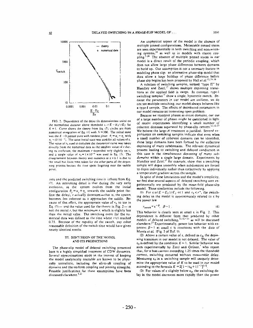
DELA YED SWITCHING IN A PHAS&SLIP MODEL OF .. 5591
10000
1000
-rswitch
0.0001 0.001 O.Q! 0.1
~ FIG. 2. Depende:nce: af Ihe dday (in dLmensionless units) on
Ihe: nonnalized distance above thresbold E =.IE - ET l/ET for K = I. Curwe shows Iht theory fro m Eq. 171; ci rcles are from numenealmlegration af Eq. (IJ wllh :Ii =300. Tbe mirial stale W3S Ihe E = 0 pmned SIOlte with random Jitter: e .. =L'lJ +1JJ with 1) 1 - o ( 10 - "). The ~me initial stat e was used for all values of t. The value o; rn used IO calculate (he theoretica l c urve was taken direclly from the numeneal data as the smaJlesl value of , durlog lis evolutIOn; tht minimum r depcnded Vtry shghtly on t, and .l single \·alue of ' 0 = I X 10-· was uSt:d in Eq. 17l. TIle dl~gr~mem betwe(>n (hen ry and numenes at c > O. I is due to tht ~mail but finite time taken for the olher pan s a f Ihe dep.n. ntog process besid!::s the time spc=ot lingenng ncar Ihe saddle pnllll.
lero and the predicted switching time is infinit e from E.q . 17) . An interesting detail is th at during the very early evolution, as Ihe system evoh'es from Ihe initial con figur at ion ej =Uj + 7J
J lowards the saddle poi nt (bt·
fore the delay), r actually decreases-that is, the system becomes less coherenl as it approaches the saddie. Be· cause a f this effect, the appropriate value of ro Io use in Eq. (7) - and Ihe vaJue used fo r the Iheory in Fig . 2- is not the initial r. but the minimum r, which is slightly less than the initial value. The switching even! for the numerical data was defined as Ihe lime where r t l ) reached 0.75. Because a f tht rapidity of the switch. any Ol her reasonable definition of the switch time would have given nea rly identical results.
III. DlSU·SSIOS OF THE :\IODEL A~D ITS PREDlc no:"liS
The phase-slip model a f dela yed switching presented here is a high ly simplilied trealment of CDW dynamics. Several approximations made in the interest a f keeping the model analyticaHy tractable are known to be pbysi · ca Ily unrealistic. including the all-to-all caupling of domains and Ihe uniform coupling and pinning strengths. PassIbie justificaI ions for these assumptions have been disc ussed elst:where.s.l~
- 250-
An unphysical aspecl a f [he model is the absence af multiple pinned configurations. Metastable pinned states are s~ experimentally in both switching and nonswitdl· ing systems,B as well as in models wilh eJastic eau· pling .~· ZI:l The absenc~ of multiple pinned stat~ in our model is a direct result a f the periodic coupling, which does not ailow large phase differences belween domams to bUI Id up. Our assumplion is nOl a necessary (cam re in modeling phase sli p: an alternative phase-slip model that does allowalarge buildup af phase difference befa re phase slip begins has been proposed by Hall el al. 12, U. lb
A subclass af switching samples. termed ·'type Il " by Hundley and Zenl, p shows multiple depinning transitions as Ihe applied field is swept. In conlrast. type·l switching samples:7 show a single, hysteretic swit ch. Be· cauS(: the parameters in o ur model are uniform. we do not see multiple switching; OUT model always behaves hk e a type-I sample. The effects af distributed parameters in our model remai ns an interesting open problem.
Because we inlerpret phases as enlire domains. ou r use af a large number af phases might be questioned in ligh t af recent experiments identifying a small number af coherent domains separated by pbase.slip centers. ll.13. 17 We btlieve the large·'" treatment is juslified: Several experiments an SWItching samples indicate that even when a smaU number af cohertnt domains ean be identified. these large domains have betn fonnet! by tbe collecti .. ·e depinoing of many subdomains. The relevant d ynamical process leading to switching and delayed conduct ion in this case is the simultal/eous dep/nl/ing o/ marty sub. domOirts within a single large domain. Experiments by Hundley and Ze ttl ,17 for example, show Ihat a switching sample will depm smoothly when subdomains a re farced to depin indiv idually rathc:r than collectively by applymg a temperature gradient across tbe sample.
In spile af these limitat ions and the moder s slmplici ly. we find that several aspectS af delayed swnchlOg seen ex · perimentally are produeed by the mean-field phase-slip modeJ. These similarilies incJude Ihe follo\\'ing.
Ol For ( ;;;:(E - E T)/Et« l and r Q <,·, the switch. ing delay in the model is approximat ely related to E by the power law
:"."UCII :r E - 8, {3- I tSi
This behavior is cJearly seen at small E in Fig. 2. This dependence is different from that predicted by other models af delayed switching,Il· lb - :1 as will be discussed elsewhere."1 Experimencally. power ·law behavior with ex.ponent (3-1 at small E is consiSlent with tbe data of Maeda el al. IF ig. 5 of Ref. 9).
(2) Aba Ye a certain value a f E . defined as f o• the depinniog transition in our model is not delayed. The value af EO is dc:fined by the condition E = L Similar behavior was seen e;r;perimc:ntally by Zettl and Griiner,' who repart thaI, for a bias curtent exceeding L2S times the threshold current, switching occurred without measurable dela y. Measuring EO in a switching sample will uniquely determine the appropriate value af K to be used in our model according to the fonnula K =2{ l-j EO + 11- 1 ]1 / 2.
(3) For values of E slightly below EOo the switching dela)' in the model decreases more rapidly than the power

5592 C. M. MARCUS, S. H. STROOAT"l. AND R. M. \VESTERVELT
law (8), giving a. concave-downward shape to a log-log plot af is.,,,"!: ... ersus t. as seen in Fig. 2. This feature IS
30150 seen in tht: e:o.perimental data af Maeda et al. (Fig 5. R,r. 91.
(4) The switching dda)' in our model de~nds an an in· itial coherence. In Eq. m this dependenee appears as the '0 term in (bt: logarithm. mdicating that a siuble initial coherence wiU shorten tht: delay. For a sufficient!y large initial coherence 'o> r·, Eq. (7) is not applicable because the cubic lcnn in Eq. 161 will dominale throughout tbt: evolution. leading to an cxtremely shon switching delay. A reduelion af tht: switching delay duc to an organized initial state has been observed indirectly in tbe cxperi· m~nts af Kriza et al.! Using two dose!y spaced su~rthleshold pulses, Kriu et al. a were able to reduce the switching delay for tbe depinning wh.ich occurred during the second pulse: the shorter the spacing bctween tbe pulses, Ihe shorter Ibe observed SWitching delay.
(,5) The delay in our model is a detenninistic funclion ol' E. K, and "0; we do not predicl a scatler In Ibe ol>served switching delay near threshold. Probabilistic models of depinning, for example. Ihe modelof Joa!> and Murray,21 predict ascaller of dday limes. A sizable scalter was repoTted by Zettl and Gruner:' more recent ly,
IChorxt! Denslry Wa"es in Solids. Vol. 217 of L ('efure NoftS in Ph}'SICl . edi led by G. HUliray and 1. S61)'om ISpnnger. Berlm. 1985\
~ For a recent feview nf charge·dcn~i t y-wa\le dynamics. see G. Gruncr. Re~· ..... 1od. Phys. 60. 112911988:.
JH. Fukuyama :lnd P. A. Lt:c. Phys. Re~·. B 17. ~J5 [197111; P. A. Lee and. T. ~f. Rice. Ibid. 19. J9iO \19791; L. Sncddon. M. C. eross. and D. S. Fisher, Phys. Rev. Lelt. 49. 292 11982l.
~L Sneddon. Phys. Re\' . 8 30, 2974 iI98~1. ~D. S. Fisher, Phys. Rev. Len. SO. 1486 1\9831; Ph~'S. Rev. B Jl.
1.39611985). liG. Gruoer. A. Zaw3dowslr::i. and P. M . Chaikm. Phys. Re~.
Len. 46. 511 (1981), 'TA. Zettland G. Grliner. Ph ys. Rc~-. B 26. 2:~98 11982 1. ~G . Kriu. A . JanDSSY. and G . Mihaly. in Charge D.'n~jry WQL't'S
In SQ/id5. Ref. 1. p. 426. ~A. ~iaeda. T. FuruY:lma. and S. Tanaka. SoILd S[ale Commun.
SS. 95 t (19851. NOle [haIIhe graph ior Fig. 5 is mcorrect ly printed as Fig. 3 in thi ~ paper.
[oJ. Dumas. C. Schlenker. J . ~arcus. and R. Buder. Phys. Re\'. Lelt. SO. 757 (]98] ): H. \futka. S. Bouffard. J . Dumas, and C. Schlcnker. J. Phys. IParisl Lell . 45. l i~9 (19841; S. &)uffard. M. Sanquer. H. Mutka. J. Dumas. and C. Schlenhr, in Charge DCrls/ry WaL't's In Solids . Rd. l, p. ~9 .
li R. P. Hall. M. F. Hundley. and A. Zeftl. Ph}'~. Re ~ . lell. S6. 2J9Q ( '9R6J.
12R. P. Hall. M. F. Hund1ey . and A. Ze1l1. Physlca B+C 14.38. 15211986),
- 251 -
K riza et al. ~ attribuled all seatter in rhe measured dday to " instrumental instabllity ." It IS not cleaT whether Ihe seaner seen experimenlally is an artifacI ar an inlrinsic feature af delayed switching.
In conclusion. we have analyzed a very simple model af CDW domain dynamlcs with phase slip. and have found several features seen experimentaJly in switching samples. The resuhs sugges{ that switching, hysleresis. and delayed anset af conductlon are dasely related phenomena which appear together when phase sHp betwcen dom3.ins occurs. Further expenmentS an delayed switching wouJd lH= very useful IO lest in greater detail thc predictive power of such a simple model.
ACK~OWLEDGME"iS
We thank Mark Sherwin for belpful discusslOns. One af us (C.M.M.l acknowledges partlal support by AT&T Bell Laboratories. and another af us IS.H.SJ acknowledges financlaJ support from thc U.S. National Science Foundation <NSF>- This research was supported in part by the U.S. Offiee af Naval Research \ON'R l under ContractS No. NOOOI4-84-K..{)465 and No. ~OOOI4-84-K-OJ29.
UR. p, Hall. \1. F. Hund/ey. and A. Zeltl. Phys . Rc ~. B 38. IJ 002 ! 1988).
14R. P. Hall and A. Zelt!. Phvs. Rev. BJ8. 13019 n988) . 15M . S. Sherwin, A. Zett1. ~nd R . P. Hall. Phys. Rev. B 38.
13 028 ti 9881. IbM. (nui. R. P. Hall. S. DOOlach , and A. Zt: III , Phy~. Rev. B 38.
I.}(H7 (]9 881. I'~ . F. Hundky and A. Zenl. pnys . Rev. B 37. 1!P!7 (JQ88'l. !lIG . Mihaly , G . Knza. and A. Jilnossy. Ph)'s. R.:'~. B 30, 3578
11984l.
19A . Janossy. G. Mihaly. !lnd L. Mih.ily. In Ch"rge Deru/ry WaL'('$ in So/Jds. Ref. !, p. 412.
laL Mihaly. Ting ehen. and G. Gruner. Sulid SUle Commun. 61. 75J 0987J.
21B. Joos and D. Murray. Phys. Rev . B 29. [094 ' 19841 !~S. H. StJogatz. C. M. Marcus. R. M. Wt:surveh. and R. E.
Mirollo. Phy!.. Rev. leu. 61,1380 119881. DS. H. Strogatl . C. M. Marcus. R. M . Wt:stervelt, and R . E.
MirolID. Physlca D 36, 23 ([981}). Hp. f. Tua and A. Zawadowd(.j, Solid StOlle Commun. 41). 19
09841. HR. J. Cavil. R. J. Fleming, E. A. Rietman. R. G. Dunn, and L.
F. Schneemeyer. fhys. Rev. lm. SJ. 167711 984); L f\.hha ly. K.-R lee. and P W. Stephens. Phys. Re~·. B 36. 1']9) {]9871.
~lIp . B. Li1llewood. Phys. Rev. B 33, 6694 11986i: Physica D 23, 4S 119861.
Z'S. H. Strogatz and R. M. Weslcrvelt. Phys. Rev. B ho ~ publi!.hedJ.