Embed Size (px)
Citation preview
Dynamics
James Sparks, Hilary Term 2020
About these notes
These are lecture notes for the Prelims Dynamics course, which is a first year course in the math-
ematics syllabus at the University of Oxford. In putting together the notes I have drawn freely
from the enormous literature on the subject; most notably from previous lecture notes for this
course (due to David Acheson and Jon Chapman) and the reading list, but also from many other
books and lecture notes. The notes are unchanged from last year.
Oxford mathematics students studying Dynamics will have taken a first course in geometry, cov-
ering the elementary ideas of the geometry of Euclidean space, including invariance under orthogo-
nal transformations, and a first course in calculus, in particular covering simple ordinary differential
equations. Some familiarity with these topics will hence be assumed. Starred sections/paragraphs
are not examinable, either because the material is slightly off-syllabus, or because it is more diffi-
cult. There are eight (short) problem sheets. Please send any questions/corrections/comments to
Contents
1 Newtonian mechanics 4
1.1 Space and time . . . . . . . . . . . . . . . . . . . . . . . . . . . . . . . . . . . . . . 4
1.2 Newton’s laws . . . . . . . . . . . . . . . . . . . . . . . . . . . . . . . . . . . . . . . 5
1.3 Dimensional analysis . . . . . . . . . . . . . . . . . . . . . . . . . . . . . . . . . . . 8
2 Forces and dynamics: a first look 10
2.1 Gravity and projectiles . . . . . . . . . . . . . . . . . . . . . . . . . . . . . . . . . . 10
2.2 Fluid drag . . . . . . . . . . . . . . . . . . . . . . . . . . . . . . . . . . . . . . . . . 12
2.3 Hooke’s law for springs . . . . . . . . . . . . . . . . . . . . . . . . . . . . . . . . . . 14
2.4 Particle in an electromagnetic field . . . . . . . . . . . . . . . . . . . . . . . . . . . 16
3 Motion in one dimension 19
3.1 Energy . . . . . . . . . . . . . . . . . . . . . . . . . . . . . . . . . . . . . . . . . . . 19
3.2 Motion in a general potential . . . . . . . . . . . . . . . . . . . . . . . . . . . . . . 22
3.3 Motion near equilibrium . . . . . . . . . . . . . . . . . . . . . . . . . . . . . . . . . 24
3.4 * Damped motion . . . . . . . . . . . . . . . . . . . . . . . . . . . . . . . . . . . . 28
1Many thanks to Pietro Benetti Genolini and Agniete Geras for comments on the first version of these notes.
1

3.5 Coupled oscillations . . . . . . . . . . . . . . . . . . . . . . . . . . . . . . . . . . . 30
4 Motion in higher dimensions 35
4.1 Planar motion in polar coordinates . . . . . . . . . . . . . . . . . . . . . . . . . . . 35
4.2 Conservative forces . . . . . . . . . . . . . . . . . . . . . . . . . . . . . . . . . . . . 36
4.3 Central forces and angular momentum . . . . . . . . . . . . . . . . . . . . . . . . . 38
5 Constrained systems 41
5.1 Constraint forces . . . . . . . . . . . . . . . . . . . . . . . . . . . . . . . . . . . . . 41
5.2 The simple pendulum . . . . . . . . . . . . . . . . . . . . . . . . . . . . . . . . . . 42
5.3 Motion on a surface under gravity . . . . . . . . . . . . . . . . . . . . . . . . . . . 45
6 The Kepler problem 50
6.1 Inverse square law forces and potentials . . . . . . . . . . . . . . . . . . . . . . . . 50
6.2 The Kepler problem and planetary orbits . . . . . . . . . . . . . . . . . . . . . . . 55
6.3 Kepler’s laws . . . . . . . . . . . . . . . . . . . . . . . . . . . . . . . . . . . . . . . 63
6.4 Coulomb scattering . . . . . . . . . . . . . . . . . . . . . . . . . . . . . . . . . . . . 64
7 Systems of particles 66
7.1 Galilean transformations . . . . . . . . . . . . . . . . . . . . . . . . . . . . . . . . . 66
7.2 Centre of mass motion . . . . . . . . . . . . . . . . . . . . . . . . . . . . . . . . . . 66
7.3 The two-body problem . . . . . . . . . . . . . . . . . . . . . . . . . . . . . . . . . . 70
8 Rotating frames and rigid bodies 72
8.1 Rotating frames . . . . . . . . . . . . . . . . . . . . . . . . . . . . . . . . . . . . . . 72
8.2 Rigid bodies . . . . . . . . . . . . . . . . . . . . . . . . . . . . . . . . . . . . . . . . 75
8.3 Simple rigid body motion . . . . . . . . . . . . . . . . . . . . . . . . . . . . . . . . 81
8.4 Newton’s laws in a non-inertial frame . . . . . . . . . . . . . . . . . . . . . . . . . 85
8.5 * The Coriolis force . . . . . . . . . . . . . . . . . . . . . . . . . . . . . . . . . . . 91
2

Preamble
Newtonian mechanics, as first developed by Galileo and Newton in the 17th century, is an extraor-
dinarily successful theory. Its laws are clear and relatively simple to state, but are applicable to
an enormous array of dynamical problems. They are also valid over a vast range of scales. For
example, in these lectures we’ll see that Newton’s laws govern phenomena as diverse as the motion
of bodies through fluids, charged particles moving in electromagnetic fields, the motion of rigid
bodies under gravity, and perhaps most famously the orbits of planets in our solar system. There
are also the slightly more mundane examples: masses attached to springs and rods, marbles rolling
on surfaces, beads sliding on wires, etc. For applied mathematicians the ideas and techniques de-
veloped in Newtonian mechanics have wide applicability, from phenomena in dynamical systems,
such as resonance and chaos, to e.g. the mathematical modelling of biological systems.
Newton’s laws nevertheless have their limits. For physics at the atomic scale classical mechanics
is replaced by quantum mechanics, while for phenomena involving speeds approaching the speed of
light one needs Einstein’s theory of relativity. However, these are much more complex descriptions
of Nature. Since for scales of everyday experience these theories agree with Newtonian mechanics,
to a good approximation, they are simply not needed to accurately describe many phenomena. In
quantum mechanics and relativity many concepts in Newton’s theory are modified: the concepts
of space and time, the notion of a particle trajectory, and even the basic process of measurement,
are all radically altered. Nevertheless, many features of Newtonian mechanics appear to be fun-
damental. In particular, the laws of conservation of energy, momentum and angular momentum
developed in this course are in some sense universal, and pervade all of theoretical physics.
3
1 Newtonian mechanics
1.1 Space and time
In Newtonian mechanics space is described by Euclidean geometry. In order to make this precise
we introduce the notion of a reference frame.
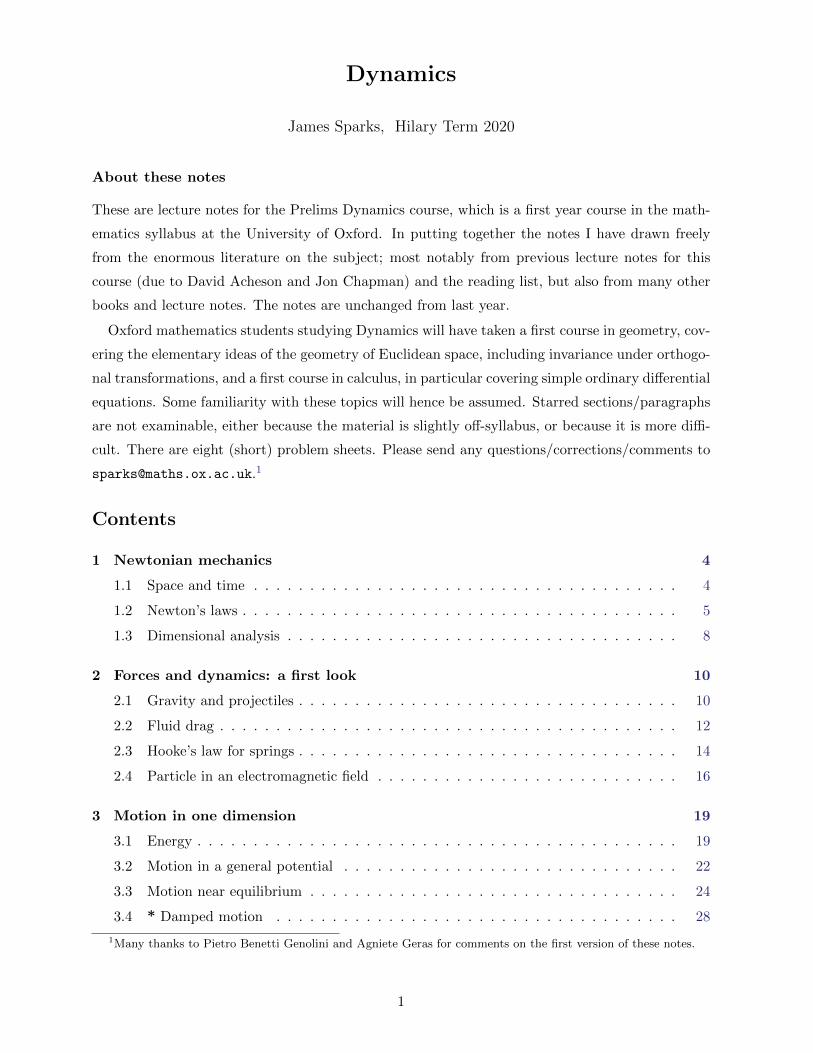
Definition A reference frame S is specified by a choice of origin O, together with a set of per-
pendicular (right handed) Cartesian coordinate axes at O.
z
r
O
axis
x axis
P
y axis
y
x
z
Figure 1: The position vector r = (x, y, z) of a point P , as measured in a reference frame S.
With respect to S a point P is specified by a position vector r from O to P . The chosen Cartesian
coordinate axes allow us to write r in terms of its components r = (x, y, z). The Euclidean
distance between two points P1, P2 with position vectors r1 = (x1, y1, z1), r2 = (x2, y2, z2) is
|r1 − r2| =√
(x1 − x2)2 + (y1 − y2)2 + (z1 − z2)2.
For many problems there may be a natural or convenient choice of reference frame, although this
is not always the case. An important assumption in Newtonian mechanics is that any two observers,
using any choice of reference frames, agree on their measurements of distances – provided they use
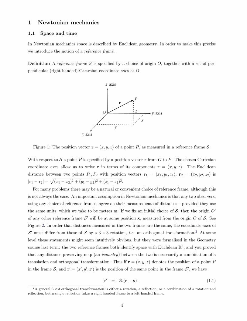
the same units, which we take to be metres m. If we fix an initial choice of S, then the origin O′
of any other reference frame S ′ will be at some position x, measured from the origin O of S. See
Figure 2. In order that distances measured in the two frames are the same, the coordinate axes of
S ′ must differ from those of S by a 3 × 3 rotation, i.e. an orthogonal transformation.2 At some
level these statements might seem intuitively obvious, but they were formalised in the Geometry
course last term: the two reference frames both identify space with Euclidean R3, and you proved
that any distance-preserving map (an isometry) between the two is necessarily a combination of a
translation and orthogonal transformation. Thus if r = (x, y, z) denotes the position of a point P
in the frame S, and r′ = (x′, y′, z′) is the position of the same point in the frame S ′, we have
r′ = R (r− x) , (1.1)
2A general 3 × 3 orthogonal transformation is either a rotation, a reflection, or a combination of a rotation andreflection, but a single reflection takes a right handed frame to a left handed frame.
4

where R is a 3× 3 orthogonal matrix. Recall these are characterized by RT = R−1.
frame S
x
y
zx
'
x
y
z
'
'
'
O
O
'
frame S
P
r
r
'
Figure 2: Relative to a choice of reference frame S, the origin O′ of another reference frame S ′ hasposition vector x, and the coordinate axes of S ′ differ from those of S by a rotation.
In order to describe dynamics we also need time. In Newtonian mechanics there is a notion
of absolute time: provided any two observers use the same units of time, which we take to be
seconds s, they will always agree on the time interval between any two events. This means that
the time variables used by two different observers are related by t′ = t − t0, and they are always
free to synchronize their clocks to set t0 = 0.
Returning to the two reference frames in Figure 2, the origins O, O′ may move relative to each
other, so x = x(t), and the axes may also rotate, so the orthogonal transformation R = R(t) is
time-dependent. We shall describe rotating frames in much greater detail in section 8.
1.2 Newton’s laws
Many dynamical processes in the real world are clearly very complicated. Mathematical mod-
els of dynamical systems usually involve making various approximations, or idealizations, in the
description of the system. One usually wants to construct the simplest model that captures the
most important features of the dynamics. Most of this course will focus on the dynamics of point
particles. These are objects whose dimensions may be neglected, to a good approximation, in
describing their motion. For example, this is the case if the size of the object is small compared
to the distances involved in the dynamics; e.g. the motion of the Earth around the Sun may be
described very accurately by treating the Earth and Sun as point particles. On the other hand, it’s
no good treating the Earth as a point particle if you want to understand the effects of its rotation!
Definition A point particle is an idealized object that at a given instant of time t is located
at a point r(t), as measured in some reference frame S. The velocity of the particle is v =
ddtr = r = (x, y, z), where a dot will denote derivative with respect to time. Its acceleration is
a = ddtv = r = (x, y, z).
5

Example (Motion with constant acceleration): Consider a particle moving in a straight line with
constant acceleration a. Let us orient our axes so that a = ak, where k is a unit vector in the
increasing z direction. Suppose that the particle starts at time t = 0 at the origin and has initial
velocity u = uk.
The constant acceleration condition is a second order differential equation for r(t), namely
r = ak. In Cartesian coordinates this reads (x, y, z) = (0, 0, a). Integrating this equation once
with respect to time t gives
r = a tk + c , (1.2)
where c is a vector integration constant. The initial condition that r(0) = u = uk then determines
c = uk. Integrating (1.2) again with respect to time t gives the solution
r(t) =(
12a t
2 + u t)
k = (0, 0, 12a t
2 + u t) . (1.3)
Here we have used the initial condition that the particle starts at time t = 0 at the origin, so
r(0) = 0, to determine the second vector integration constant. �
As time evolves the position of the particle sweeps out a curve r(t), parametrized by time t,
which we refer to as the trajectory. This must satisfy Newton’s laws of motion for point particles,
but before discussing these we need another definition.
Definition A point particle has a (inertial) mass m > 0. We measure mass in kilograms kg. Its
momentum (or more accurately linear momentum) is p = mv = mr.
In section 1.1 we noted that there are many choices of reference frames. Newton’s first law singles
out a special class of reference frames, called inertial frames.
N1: In an inertial frame a particle moves with constant momentum, unless acted on
by an external force.
In this course we will only consider constant mass particles, so that constant momentum p = mv
means constant velocity v. This is also sometimes referred to as uniform motion in a straight line.
Suppose I choose a reference frame S: how do I know it is inertial? According to N1 it is inertial
if a particle with no identifiable forces acting on it travels in a straight line with constant speed
v = |v|. But how do we know whether or not there are any forces acting? And indeed, what is
a force?! We will begin to introduce and study forces in section 2, but an essential point is that
forces arise from the presence of other matter, which our particle interacts with. Thus one way to
ensure there are no forces acting is to head deep into space, far away from any other matter. This
is not very practical. On the surface of the Earth every particle experiences the force of gravity.
However, for a particle sitting on a solid surface the force due to gravity (its weight) is balanced
6
by a normal reaction force of the surface pushing back on the particle. There is hence no net force
acting on the particle, and the fact that it doesn’t move demonstrates that a frame rigidly fixed
relative to the surface of the Earth is a very good approximation to an inertial frame.3 Whenever
we refer to an “inertial frame”, we usually have in mind such a frame fixed to the Earth’s surface.
What about non-inertial frames? We shall describe these in much more detail in section 8, but
it might be helpful here to make a few, hopefully intuitive, comments. Relative to an inertial frame
S, a non-inertial frame S ′ will either have: (i) the origin O′ accelerating with respect to O, or (ii)
the axes of S ′ rotating relative to the axes of S. In a non-inertial frame a particle will appear to
be acted on by “fictitious forces”, in addition to any actual forces in Newton’s second law stated
below. For example, consider an observer standing inside a train carriage, with reference frame
S ′ fixed relative to the interior of the train. As the train pulls out of a station it accelerates,
and the origin O′ of S ′ is likewise accelerating. The person inside the train (and everything else!)
feels like they are being thrown backwards: this isn’t a real force in Newton’s equations, but a
fictitious force due to the frame S ′ being non-inertial. Similarly, consider an observer standing on
a roundabout, whose frame S ′ rotates with the roundabout about a fixed vertical axis. As most
of us will have experienced, you feel like you are being thrown outwards, away from the axis of
rotation.
In an inertial frame, the dynamics of a point particle is governed by
N2: The rate of change of linear momentum is equal to the net force acting on the
particle: F = p.
Assuming the mass m is constant the right hand side of Newton’s second law is p = mr, and this
is the vector form of the familiar “F = ma”. The inertial mass m of a particle hence measures its
resistance to accelerate when subjected to a given force F. This external force might in general
depend on the particle’s position r, its velocity r, and on time t, so that F = F(r, r, t). Newton’s
second law is then a second order ordinary differential equation (ODE) for r(t):
F(r(t), r(t), t) = m r(t) . (1.4)
This is also often referred to as the equation of motion for the particle. Since (1.4) is second order,
for “suitably nice” functions F(r, r, t) one expects that specifying the position r and velocity r at
some initial time t = t0 gives a unique solution for the particle trajectory r(t). A central problem
in Dynamics is to find this trajectory, for a given force F.
Finally, if we have more than one particle, then
N3: If particle 1 exerts a force F = F21 on particle 2, then particle 2 also exerts a force
F12 = −F on particle 1.
3Actually it is not quite inertial: the Earth rotates around its axis once per day, and is accelerating due to itsmotion around the Sun once per year. The former leads to a measurable effect, as we shall see in section 8.5.
7
In other words, F12 = −F21. This is often paraphrased by saying that every action has an equal
and opposite reaction.
1.3 Dimensional analysis
The fundamental dimensions in mechanics are length L, time T and mass M.4 A square bracket is
usually used to denote the dimension of a variable, so that [length] = L, [time] = T, [mass] = M.
Dimensions of other quantities may then be derived from these. For example, the dimensions of
velocity are [r] = L T−1.
A given dimension may be measured in a number of different standard units. For example,
length might be measured in inches, metres or light-years (the distance light travels in a year in
vacuum). There is then a scaling factor to convert between different units, e.g. 1 metre ' 39.4
inches, 1 light-year ' 9.46× 10¹⁵ metres, etc. In order that equations in physics are independent
of the choice of units, which after all are arbitrary, it’s important that the dimensions of both sides
of an equation are the same. Similarly, we may only add two quantities if they have the same
dimensions.
Example (Dimensions of force): Newton’s second law gives the dimensions of force as [F] =
M L T−2. The magnitude |F| is measured in Newtons N, where 1 N = 1 kg m s−2. �
More interestingly, a knowledge of the dimensions of the parameters in a problem can sometimes
be used to construct scaling laws, without needing to solve any differential equations.
Example (Maximum height for constant acceleration): Let’s reconsider the example of constant
acceleration in section 1.2. For a particle moving along the z axis, starting at the origin at time
t = 0 with velocity u = uk, we showed that the trajectory is r(t) = (12at
2 + ut) k. Suppose that
u > 0 but the constant acceleration a = −g < 0 is negative; that is, the particle starts out moving
in the positive z direction, but is accelerating in the opposite direction. In this case it will reach
a maximum height zmax at a time tmax, when r(tmax) = 0:
0 = r(tmax) = (−g tmax + u) k =⇒ tmax =u
g. (1.5)
We then compute
zmax = −1
2g t2max + u tmax =
u2
2g. (1.6)
The dimensionful quantities in the problem are u, with [u] = L T−1, and g, with [g] = L T−2. The
only way to obtain quantities with dimensions of T and L, respectively, are hence as[u
g
]=
L T−1
L T−2= T ,
[u2
g
]=
L2 T−2
L T−2= L . (1.7)
4When we discuss problems in electromagnetism we will also need to add electric charge Q.
8
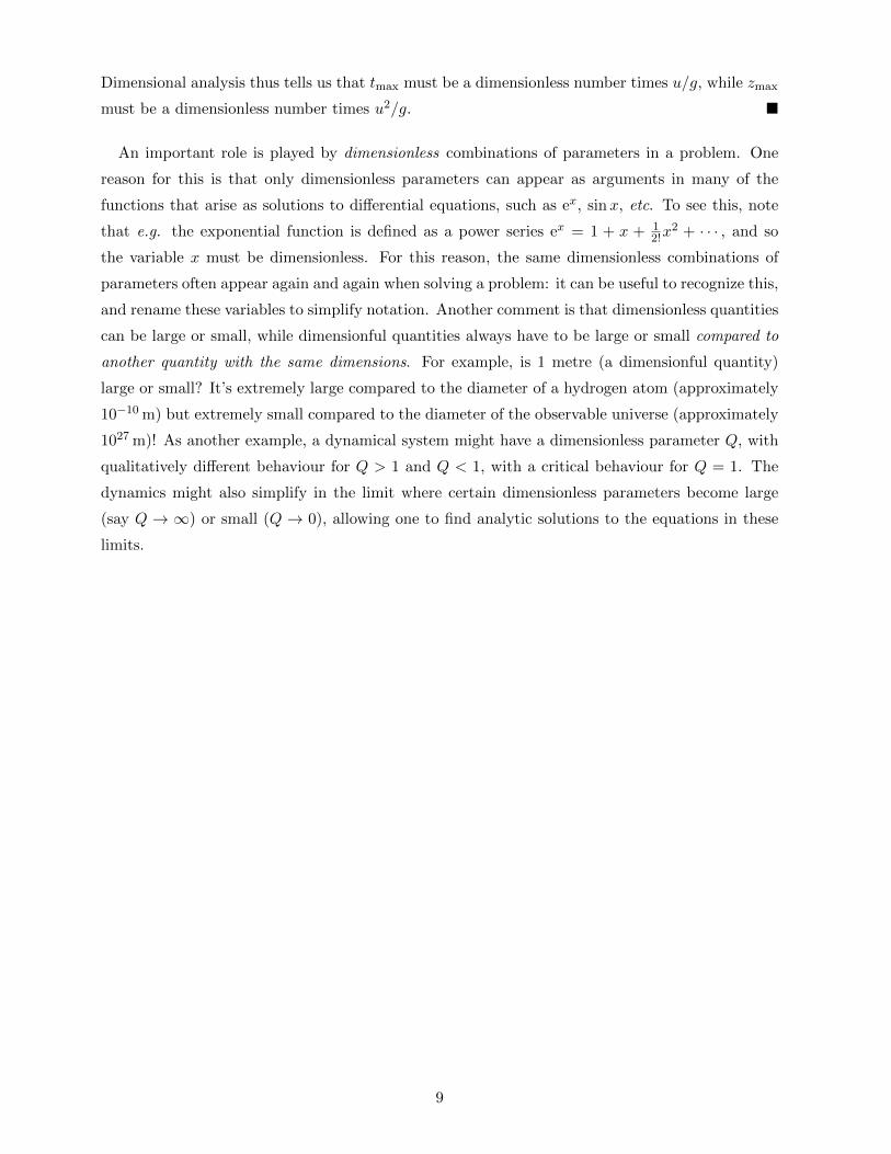
Dimensional analysis thus tells us that tmax must be a dimensionless number times u/g, while zmax
must be a dimensionless number times u2/g. �
An important role is played by dimensionless combinations of parameters in a problem. One
reason for this is that only dimensionless parameters can appear as arguments in many of the
functions that arise as solutions to differential equations, such as ex, sinx, etc. To see this, note
that e.g. the exponential function is defined as a power series ex = 1 + x + 12!x
2 + · · · , and so
the variable x must be dimensionless. For this reason, the same dimensionless combinations of
parameters often appear again and again when solving a problem: it can be useful to recognize this,
and rename these variables to simplify notation. Another comment is that dimensionless quantities
can be large or small, while dimensionful quantities always have to be large or small compared to
another quantity with the same dimensions. For example, is 1 metre (a dimensionful quantity)
large or small? It’s extremely large compared to the diameter of a hydrogen atom (approximately
10−10 m) but extremely small compared to the diameter of the observable universe (approximately
1027 m)! As another example, a dynamical system might have a dimensionless parameter Q, with
qualitatively different behaviour for Q > 1 and Q < 1, with a critical behaviour for Q = 1. The
dynamics might also simplify in the limit where certain dimensionless parameters become large
(say Q → ∞) or small (Q → 0), allowing one to find analytic solutions to the equations in these
limits.
9
2 Forces and dynamics: a first look
In this section we introduce a number of different forces, and solve Newton’s second law (1.4) to
find the particle trajectory r(t). In some cases more than one force may be acting on the particle.
Forces are vectors, and the total force acting is simply the sum of all forces. Explicitly, if forces
F1,F2, . . . ,Fn all act on a particle, the force F appearing in Newton’s second law is the vector
sum
F =n∑i=1
Fi . (2.1)
2.1 Gravity and projectiles
A particle of mass m near the Earth’s surface experiences a gravitational force mg vertically
downwards, where g ' 9.81 m s−2 is the acceleration due to gravity. This force is the particle’s
weight. In an inertial frame where the z axis is the vertical direction, so that the x and y axes
are horizontal, we may write the force as F = −mg k, where k is a unit vector directed upwards.
More precisely, the mass m = mG that appears in this force is the gravitational mass, which is
logically distinct from the inertial mass m = mI that appears in N2. Newton’s second law (1.4)
hence reads
−mG g k = mI a . (2.2)
It is an experimental fact that mI = mG, as demonstrated famously by Galileo throwing things
off the tower of Pisa. It follows that the acceleration a = −g k is independent of the mass (hence
the name “acceleration due to gravity” for g). In practice air resistance can make an enormous
difference when you throw two objects of the same mass, but more modern experiments confirm
that mI/mG = 1, to at least 10−12 in precision.5
Example (Vertical motion under gravity): With notation as above, consider a particle of mass m
projected from the origin at time t = 0 with initial velocity u = uk. Newton’s second law (2.2)
simplifies to r = a = −g k, which is precisely the example we solved in section 1. The solution is
r(t) =(−1
2gt2 + ut
)k . (2.3)
�
We may make this more interesting by changing the initial condition.
Example (Projectiles): Suppose that a small projectile is thrown with velocity V at an angle α
to the horizontal, from a height h above the ground. Find the curve traced out by the trajectory
of the projectile, and its horizontal range.
5** Einstein turned this around and made mI = mG into a new principle, called the Equivalence Principle. Itled him to formulate his General Theory of Relativity, in which gravity is not a force as in Newton’s theory, butrather a curvature of space (which is no longer Euclidean) and time itself.
10

z
Ox
r
i
kh
Vα
mg
Figure 3: Throwing a projectile.
We choose the origin O at ground level, and a unit vector k pointing vertically, and i horizontally
along the ground. The only force acting is gravity, with F = −mg k, so that Newton’s second law
reads
mr = −mg k . (2.4)
The initial conditions are
At time t = 0: r(0) = hk , r(0) = V = V cosα i + V sinαk . (2.5)
Integrating (2.4) twice and using (2.5) we find the solution
r(t) = −1
2g t2 k + tV cosα i + tV sinαk + hk . (2.6)
This is the trajectory of the projectile. We can find the curve that this traces out in the (x, z)
plane by eliminating time t. Writing r = x i + z k, reading off the components of (2.6) gives
x(t) = tV cosα , z(t) = −1
2g t2 + tV sinα+ h . (2.7)
Using the first equation we may solve for t in terms of x, and then substitute into the second
equation, giving
z = − g
2V 2x2 sec2 α+ x tanα+ h . (2.8)
This is a parabola.
The projectile hits the ground when z = r · k = 0. From (2.8) this gives a quadratic equation
for the horizontal range x, with solution
x =V 2 cosα
g
[sinα+
√sin2 α+ 2gh/V 2
]. (2.9)
Notice that the second solution to the quadratic, with a minus sign in front of the square root
in (2.9), has x < 0 and corresponds to continuing the trajectory backwards, before t = 0. Note
also that if we throw the projectile from ground level, so h = 0, the range simplifies to x =
(2V 2 cosα sinα)/g = (V 2 sin 2α)/g, which is maximized to xmax = V 2/g for an angle α = π/4. �
11
2.2 Fluid drag
In practice any body moving through a fluid, such as air or water, experiences an effective drag
force. This drag force is velocity dependent, with two common models being linear or quadratic
in the speed, with the force acting in the opposite direction to the velocity of the particle:
• A linear drag holds when viscous forces predominate, i.e. this is due to the “stickiness” of
the fluid. The force is
F = −b r , (2.10)
where b > 0 is a constant (the friction coefficient), and r is the particle velocity.
• A quadratic drag holds when the resistance is due to the body having to push fluid to the
side as it moves, for example a rowing boat moving through water. The force is
F = −D |r| r , (2.11)
where the constant D > 0.6
Both are effective/approximate descriptions of the actual force on a body moving through fluid.
At the molecular level the force arises due to collisions between the body and the fluid particles
(with the fluid particles also colliding with each other). These molecular forces are ultimately
electromagnetic forces.
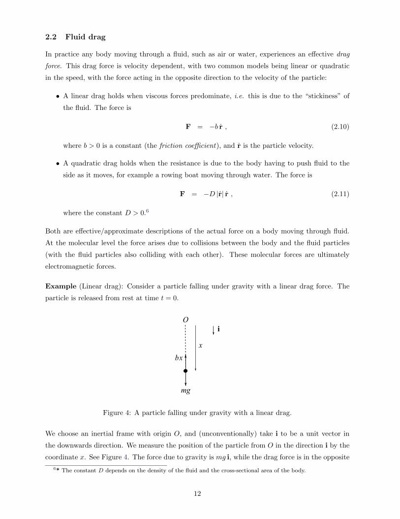
Example (Linear drag): Consider a particle falling under gravity with a linear drag force. The
particle is released from rest at time t = 0.
mg
iO
x
bx
Figure 4: A particle falling under gravity with a linear drag.
We choose an inertial frame with origin O, and (unconventionally) take i to be a unit vector in
the downwards direction. We measure the position of the particle from O in the direction i by the
coordinate x. See Figure 4. The force due to gravity is mg i, while the drag force is in the opposite
6* The constant D depends on the density of the fluid and the cross-sectional area of the body.
12
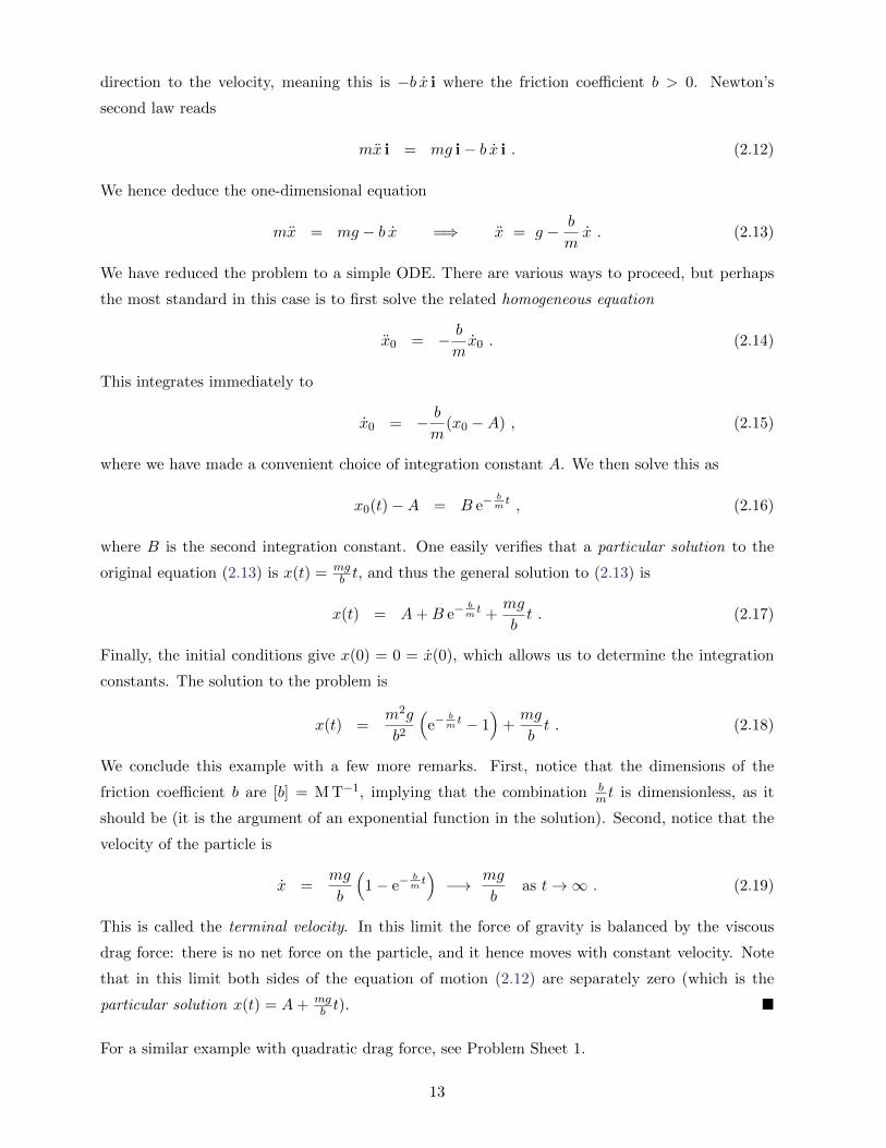
direction to the velocity, meaning this is −b x i where the friction coefficient b > 0. Newton’s
second law reads
mx i = mg i− b x i . (2.12)
We hence deduce the one-dimensional equation
mx = mg − b x =⇒ x = g − b
mx . (2.13)
We have reduced the problem to a simple ODE. There are various ways to proceed, but perhaps
the most standard in this case is to first solve the related homogeneous equation
x0 = − b
mx0 . (2.14)
This integrates immediately to
x0 = − b
m(x0 −A) , (2.15)
where we have made a convenient choice of integration constant A. We then solve this as
x0(t)−A = B e−bmt , (2.16)
where B is the second integration constant. One easily verifies that a particular solution to the
original equation (2.13) is x(t) = mgb t, and thus the general solution to (2.13) is
x(t) = A+B e−bmt +
mg
bt . (2.17)
Finally, the initial conditions give x(0) = 0 = x(0), which allows us to determine the integration
constants. The solution to the problem is
x(t) =m2g
b2
(e−
bmt − 1
)+mg
bt . (2.18)
We conclude this example with a few more remarks. First, notice that the dimensions of the
friction coefficient b are [b] = M T−1, implying that the combination bm t is dimensionless, as it
should be (it is the argument of an exponential function in the solution). Second, notice that the
velocity of the particle is
x =mg
b
(1− e−
bmt)−→ mg
bas t→∞ . (2.19)
This is called the terminal velocity. In this limit the force of gravity is balanced by the viscous
drag force: there is no net force on the particle, and it hence moves with constant velocity. Note
that in this limit both sides of the equation of motion (2.12) are separately zero (which is the
particular solution x(t) = A+ mgb t). �
For a similar example with quadratic drag force, see Problem Sheet 1.
13
2.3 Hooke’s law for springs
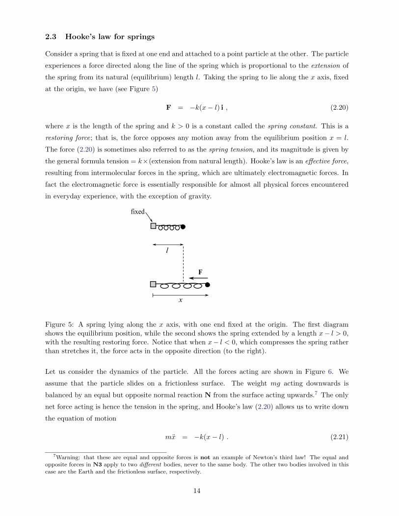
Consider a spring that is fixed at one end and attached to a point particle at the other. The particle
experiences a force directed along the line of the spring which is proportional to the extension of
the spring from its natural (equilibrium) length l. Taking the spring to lie along the x axis, fixed
at the origin, we have (see Figure 5)
F = −k(x− l) i , (2.20)
where x is the length of the spring and k > 0 is a constant called the spring constant. This is a
restoring force; that is, the force opposes any motion away from the equilibrium position x = l.
The force (2.20) is sometimes also referred to as the spring tension, and its magnitude is given by
the general formula tension = k×(extension from natural length). Hooke’s law is an effective force,
resulting from intermolecular forces in the spring, which are ultimately electromagnetic forces. In
fact the electromagnetic force is essentially responsible for almost all physical forces encountered
in everyday experience, with the exception of gravity.
l
fixed
x
F
Figure 5: A spring lying along the x axis, with one end fixed at the origin. The first diagramshows the equilibrium position, while the second shows the spring extended by a length x− l > 0,with the resulting restoring force. Notice that when x− l < 0, which compresses the spring ratherthan stretches it, the force acts in the opposite direction (to the right).
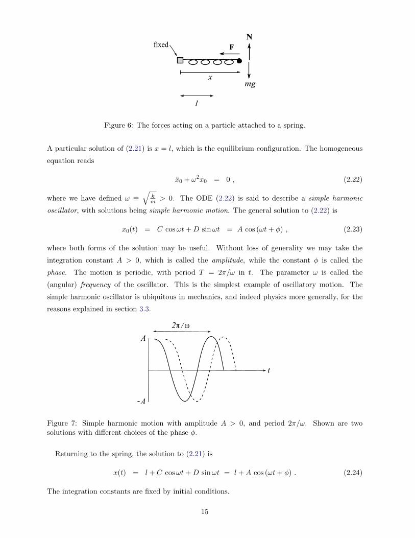
Let us consider the dynamics of the particle. All the forces acting are shown in Figure 6. We
assume that the particle slides on a frictionless surface. The weight mg acting downwards is
balanced by an equal but opposite normal reaction N from the surface acting upwards.7 The only
net force acting is hence the tension in the spring, and Hooke’s law (2.20) allows us to write down
the equation of motion
mx = −k(x− l) . (2.21)
7Warning: that these are equal and opposite forces is not an example of Newton’s third law! The equal andopposite forces in N3 apply to two different bodies, never to the same body. The other two bodies involved in thiscase are the Earth and the frictionless surface, respectively.
14
l
fixed
x
F
mg
N
Figure 6: The forces acting on a particle attached to a spring.
A particular solution of (2.21) is x = l, which is the equilibrium configuration. The homogeneous
equation reads
x0 + ω2x0 = 0 , (2.22)
where we have defined ω ≡√
km > 0. The ODE (2.22) is said to describe a simple harmonic
oscillator, with solutions being simple harmonic motion. The general solution to (2.22) is
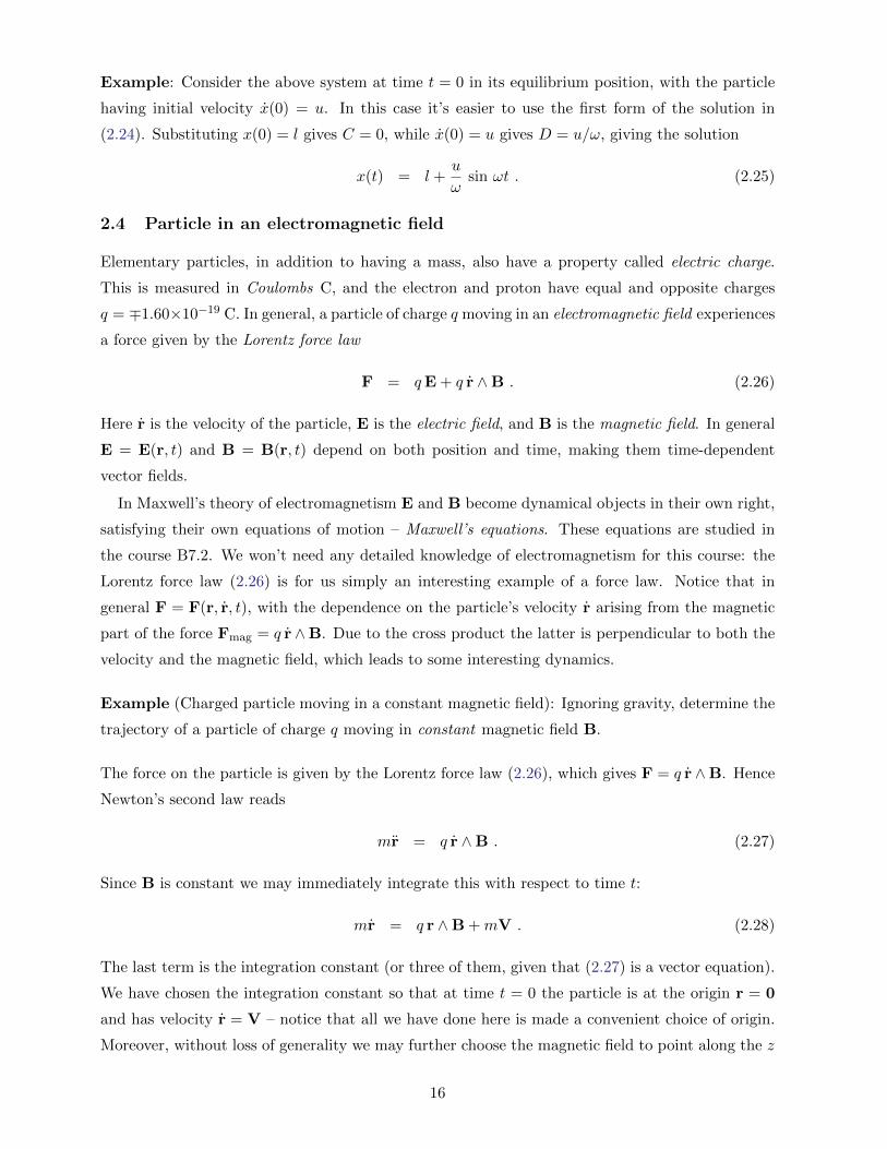
x0(t) = C cosωt+D sinωt = A cos (ωt+ φ) , (2.23)
where both forms of the solution may be useful. Without loss of generality we may take the
integration constant A > 0, which is called the amplitude, while the constant φ is called the
phase. The motion is periodic, with period T = 2π/ω in t. The parameter ω is called the
(angular) frequency of the oscillator. This is the simplest example of oscillatory motion. The
simple harmonic oscillator is ubiquitous in mechanics, and indeed physics more generally, for the
reasons explained in section 3.3.
t
A
A-
2 /π ω
Figure 7: Simple harmonic motion with amplitude A > 0, and period 2π/ω. Shown are twosolutions with different choices of the phase φ.
Returning to the spring, the solution to (2.21) is
x(t) = l + C cosωt+D sinωt = l +A cos (ωt+ φ) . (2.24)
The integration constants are fixed by initial conditions.
15
Example: Consider the above system at time t = 0 in its equilibrium position, with the particle
having initial velocity x(0) = u. In this case it’s easier to use the first form of the solution in
(2.24). Substituting x(0) = l gives C = 0, while x(0) = u gives D = u/ω, giving the solution
x(t) = l +u
ωsin ωt . (2.25)
2.4 Particle in an electromagnetic field
Elementary particles, in addition to having a mass, also have a property called electric charge.
This is measured in Coulombs C, and the electron and proton have equal and opposite charges
q = ∓1.60×10⁻¹⁹ C. In general, a particle of charge q moving in an electromagnetic field experiences
a force given by the Lorentz force law
F = qE + q r ∧B . (2.26)
Here r is the velocity of the particle, E is the electric field, and B is the magnetic field. In general
E = E(r, t) and B = B(r, t) depend on both position and time, making them time-dependent
vector fields.
In Maxwell’s theory of electromagnetism E and B become dynamical objects in their own right,
satisfying their own equations of motion – Maxwell’s equations. These equations are studied in
the course B7.2. We won’t need any detailed knowledge of electromagnetism for this course: the
Lorentz force law (2.26) is for us simply an interesting example of a force law. Notice that in
general F = F(r, r, t), with the dependence on the particle’s velocity r arising from the magnetic
part of the force Fmag = q r ∧B. Due to the cross product the latter is perpendicular to both the
velocity and the magnetic field, which leads to some interesting dynamics.
Example (Charged particle moving in a constant magnetic field): Ignoring gravity, determine the
trajectory of a particle of charge q moving in constant magnetic field B.
The force on the particle is given by the Lorentz force law (2.26), which gives F = q r ∧B. Hence
Newton’s second law reads
mr = q r ∧B . (2.27)
Since B is constant we may immediately integrate this with respect to time t:
mr = q r ∧B +mV . (2.28)
The last term is the integration constant (or three of them, given that (2.27) is a vector equation).
We have chosen the integration constant so that at time t = 0 the particle is at the origin r = 0
and has velocity r = V – notice that all we have done here is made a convenient choice of origin.
Moreover, without loss of generality we may further choose the magnetic field to point along the z
16
axis, so B = (0, 0, B), and then use the freedom to rotate the (x, y) plane so that V = (V1, 0, V3).
Writing r = (x, y, z), note that r ∧B = −xB j + yB i. Writing the integrated equation of motion
(2.28) out in components thus gives the three ODEs
mx = qB y +mV1 ,
my = −qB x ,
mz = mV3 . (2.29)
The last equation immediately solves to give z(t) = V3t (using the initial condition r(0) = 0).
Solving for x in terms of y from the second equation and substituting into the first gives a second
order ODE for y. One can solve the equations this way, but a slicker way to proceed is to introduce
the complex variable ζ = x+ iy. Specifically, taking the first equation in (2.29) and adding i times
the second equation gives the complex equation
m(x+ iy) = −qB i (x+ iy) +mV1 , (2.30)
which in terms of ζ = x+ iy reads
mζ = −qB iζ +mV1 . (2.31)
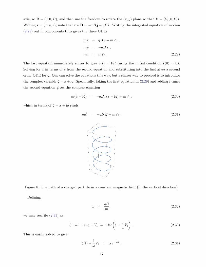
Figure 8: The path of a charged particle in a constant magnetic field (in the vertical direction).
Defining
ω =qB
m. (2.32)
we may rewrite (2.31) as
ζ = −iω ζ + V1 = −iω
(ζ +
i
ωV1
). (2.33)
This is easily solved to give
ζ(t) +i
ωV1 = α e−iωt , (2.34)
17
where α is a complex integration constant. Using the initial condition ζ(0) = 0 fixes α = iV1/ω.
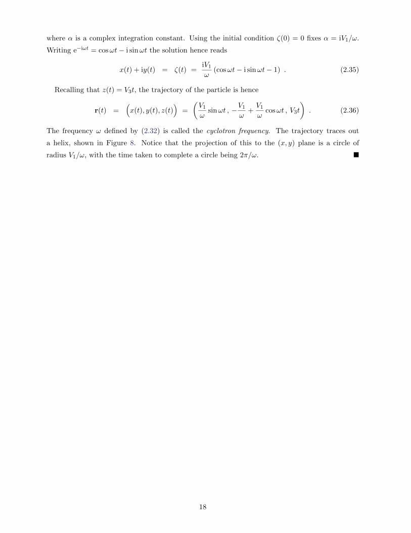
Writing e−iωt = cosωt− i sinωt the solution hence reads
x(t) + iy(t) = ζ(t) =iV1
ω(cosωt− i sinωt− 1) . (2.35)
Recalling that z(t) = V3t, the trajectory of the particle is hence
r(t) =(x(t), y(t), z(t)
)=
(V1
ωsinωt , −V1
ω+V1
ωcosωt , V3t
). (2.36)
The frequency ω defined by (2.32) is called the cyclotron frequency. The trajectory traces out
a helix, shown in Figure 8. Notice that the projection of this to the (x, y) plane is a circle of
radius V1/ω, with the time taken to complete a circle being 2π/ω. �
18
3 Motion in one dimension
In the previous section we were always able to solve Newton’s second law explicitly, in closed
form. Unfortunately, as soon as we move beyond the simplest examples, for example by combining
the effects of different forces, it becomes very difficult to solve for the trajectory explicitly. In
this section we introduce some general methods that help to understand certain aspects of the
dynamics, without having to solve Newton’s second law directly. We will here focus (mainly) on
dynamics in one dimension. Why focus on one-dimensional motion when the real world is three-
dimensional? Firstly, the problems are simpler, and when studying any new subject one should
always begin by trying to isolate the new phenomena and features in their simplest setting. But
more importantly, many three-dimensional problems may effectively be reduced to studying lower
dimensional problems.
3.1 Energy
Consider a particle moving along the x axis, subject to a force F = F (x) that depends only on
the particle’s position x. Newton’s second law gives
mx = F (x) . (3.1)
This is a second order ODE, but in this case there always exists a first integral. To see this, we
first introduce:
Definition The kinetic energy of the particle is T = 12mx
2. We may also write this in terms of
momentum p = mx as T = p2/2m. Energy is measured in Joules J, with 1 J = 1 kg m2 s−2.
To see the utility of this, we calculate
T = mx x = F (x) x , (3.2)
where the second equality uses (3.1). Suppose the particle starts at position x1 at time t1, and
finishes at x2 at time t2. Integrating (3.2) with respect to time t gives
T (t2)− T (t1) =
∫ t2
t1
T dt =
∫ t2
t1
F (x(t)) x dt =
∫ x2
x1
F (x) dx . (3.3)
This motivates another definition:
Definition The work done W by the force in moving the particle from x1 to x2 is
W =
∫ x2
x1
F (x) dx . (3.4)
Equation (3.3) thus proves:
19
Work-Energy Theorem The work done by the force is the change in kinetic energy:
W = T (t2)− T (t1) . (3.5)
�
This notion of work also leads to the following definition:
Definition The potential energy of the particle is V (x) = −∫ x
x0
F (y) dy, where x0 is arbitrary.
By definition, the potential energy V (x) is minus the work done by the force in moving the particle
from x0 to x. This a priori depends on the choice of x0, but if we change x0 7→ x0 the potential
energy changes to V (x) 7→ V (x)−∫ x0x0F (y) dy. Changing x0 thus simply shifts V (x) by an additive
constant: potential energy is understood to be defined only up to an overall additive constant.
Using the Fundamental Theorem of Calculus we may write the force as
F (x) = −dV
dx= −V ′(x) . (3.6)
Examples:
1. For F = −mg a choice of potential is V (x) = mgx.
2. For Hooke’s linear force F = −k(x− l) a choice of potential is V (x) = 12k(x− l)2.
Notice that we’ve made a natural choice of additive integration constant in each case, but any
choice will do. Also, be careful with the signs!
Conservation of Energy Theorem The total energy of the particle
E = T + V (3.7)
is conserved, i.e. is constant when evaluated on a solution to Newton’s second law (3.1).
Proof 1: From the Work-Energy Theorem we already have
T (t2)− T (t1) = W =
∫ x2
x1
F (x) dx = V (x1)− V (x2) . (3.8)
Rearranging thus gives
E = T (t1) + V (x1) = T (t2) + V (x2) . (3.9)
Since the initial and final positions and times here are arbitrary, this proves E is conserved. �
20
Proof 2: More precisely we first write the right hand side of (3.7) as T (t) + V (x(t)). Using the
chain rule we then have
E = T + V = mx x+dV
dx
dx
dt= x (mx− F ) . (3.10)
It follows that E = 0 is implied by Newton’s second law.8 �
The fact that E is constant implies that in the motion any loss of potential energy necessarily
results in an equal gain in the kinetic energy T = 12mx
2, and hence a gain in the speed |x| of the
particle (and of course the same statement with loss/gain interchanged).
Notice that we may rewrite (3.7) as
1
2mx2 = E − V (x) . (3.11)
This equation has many implications. First, knowing the energy E and position of the particle
immediately gives its speed |x|. Second, since kinetic energy T = 12mx
2 ≥ 0 is non-negative, we
always have V (x) ≤ E. This confines the possible location of the particle, for fixed energy. We’ll
see in section 3.2 that this allows us to determine the qualitative motion of particles, in a general
potential V (x). But we may also obtain quantitative information.
Example (Maximum height under gravity (again)): Let’s revisit the example in section 1.3:
consider a particle moving vertically under gravity, which at time t = 0 starts at height z = 0 with
velocity z = u > 0 upwards. What is the maximum height of the particle?
The potential is V (z) = mgz. The conserved energy E may be calculated from the initial condi-
tions, which gives E = T (0) = 12mu
2. Thus (3.11) reads
1
2mz2 =
1
2mu2 −mgz . (3.12)
The maximum height occurs when z = 0, which immediately gives
zmax =u2
2g. (3.13)
�
We may also write that the work done in moving the particle from position x0 at time t0 to position
x at time t is
W (t) =
∫ x(t)
x0
F (y) dy = V (x0)− V (x(t)) . (3.14)
8* Notice that conversely E = 0 implies Newton’s second law, unless x is zero for all time. In the latter casex = x0 is constant, and equation (3.11) then implies that E = V (x0). This solves (3.11), but Newton’s second lawonly holds if in addition F (x0) = −V ′(x0) = 0.
21
Definition Power P = rate of work done, so that
P =dW
dt= F x . (3.15)
Power is measured in Watts, with 1 Watt = 1 J s−1.
For conservative forces, meaning there is a potential satisfying (3.6), the work done by the force
in any motion can be positive or negative, in the former case causing a corresponding increase in
kinetic energy, by the Work-Energy Theorem. However, this is in general not the case for time-
dependent or velocity-dependent forces. For example, for a linear drag force F = −b x, with b > 0,
the work done by the resistive force over a small distance δx is −b x δx = −b x2 δt < 0. Thus the
work done is always negative, no matter what the motion. For a dissipative force, such as drag or
friction, energy is apparently lost. However, at a microscopic level energy should be conserved –
this is believed to be a fundamental principle in physics. In the case of fluid drag, the issue is that
we have ignored the “back-reaction” of our body on the fluid particles. In each collision between
the body and the fluid particles energy is conserved, but some of the kinetic energy is transferred
to the fluid particles, increasing their average kinetic energy. But by definition this means we lost
kinetic energy of our object as heat – the fluid will be a bit warmer.
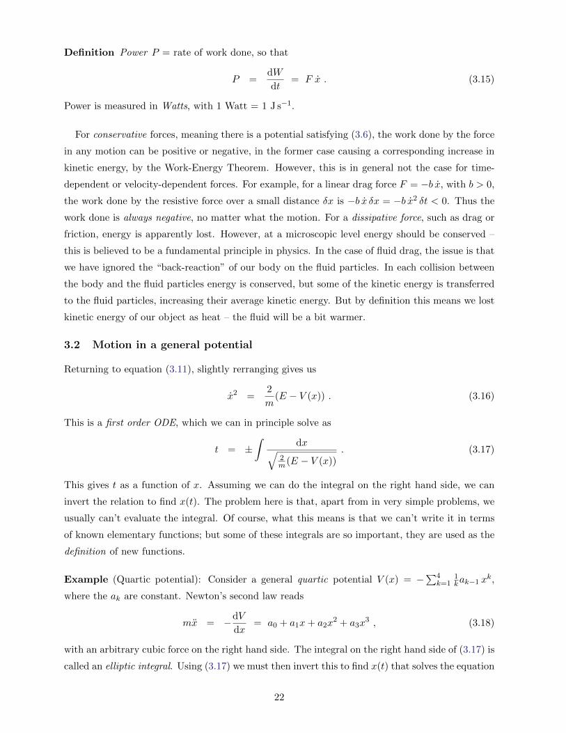
3.2 Motion in a general potential
Returning to equation (3.11), slightly rerranging gives us
x2 =2
m(E − V (x)) . (3.16)
This is a first order ODE, which we can in principle solve as
t = ±∫
dx√2m(E − V (x))
. (3.17)
This gives t as a function of x. Assuming we can do the integral on the right hand side, we can
invert the relation to find x(t). The problem here is that, apart from in very simple problems, we
usually can’t evaluate the integral. Of course, what this means is that we can’t write it in terms
of known elementary functions; but some of these integrals are so important, they are used as the
definition of new functions.
Example (Quartic potential): Consider a general quartic potential V (x) = −∑4
k=11kak−1 x
k,
where the ak are constant. Newton’s second law reads
mx = −dV
dx= a0 + a1x+ a2x
2 + a3x3 , (3.18)
with an arbitrary cubic force on the right hand side. The integral on the right hand side of (3.17) is
called an elliptic integral. Using (3.17) we must then invert this to find x(t) that solves the equation
22
of motion (3.18). The inverse of an elliptic integral is called an elliptic function. These appear
repeatedly in mathematics, and are in themselves a beautiful topic, with surprising features. �
Example (Quadratic potential – the harmonic oscillator): A special case of the former example
is a quadratic potential, with a2 = a3 = 0. We have already solved this problem in section 2.3: it
is just the spring – see equation (2.21). Let us begin with the homogeneous harmonic oscillator
equation (2.22)
x+ ω2x = 0 . (3.19)
The force acting is F (x) = −mω2x, which has a potential energy function V (x) = 12mω
2x2.
Equation (3.17) hence reads
t = ±∫
dx
ω√
2Emω2 − x2
. (3.20)
We may solve this by making the substitution
x =
√2E
mω2cos θ , (3.21)
which gives
t = ∓∫
1
ωdθ =⇒ t− t0 = ∓ 1
ωcos−1
(x√
2E/mω2
). (3.22)
Here t0 is an integration constant. The solution is hence simple harmonic motion
x(t) =
√2E
mω2cos [ω(t− t0)] . (3.23)
Notice that in this case it is easier to solve the second order equation of motion, than to integrate
the first order conservation of energy equation! On the other hand, we have learned that the
amplitude A =√
2E/mω2, c.f. equation (2.23). �
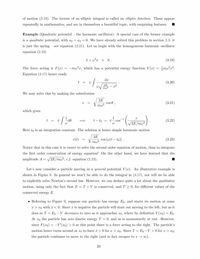
Let’s now consider a particle moving in a general potential V (x). An illustrative example is
shown in Figure 9. In general we won’t be able to do the integral in (3.17), nor will we be able
to explicitly solve Newton’s second law. However, we can deduce quite a lot about the qualitative
motion, using only the fact that E = T + V is conserved, and T ≥ 0, for different values of the
conserved energy E.
• Referring to Figure 9, suppose our particle has energy E0, and starts its motion at some
x > x0 with x < 0. Since x is negative the particle will start out moving to the left, but as it
does so T = E0 − V decreases to zero as it approaches x0, where by definition V (x0) = E0.
At x0 the particle has zero kinetic energy T = 0, and so is momentarily at rest. However,
since F (x0) = −V ′(x0) > 0 at this point there is a force acting to the right. The particle’s
motion hence turns around at x0 to have x > 0 for x > x0. Since T = E0−V > 0 for x > x0,
the particle continues to move to the right (and in fact escapes to x→∞).
23

x0 x1 xmin x2 x3xmaxx
V(x)
E0
E1
Figure 9: A general potential V (x), with various points marked on the x axis. xmin and xmax area local minimum and local maximum, respectively. At any point x the force acting on the particleis minus the slope of the potential, F (x) = −V ′(x).
• For E = E1 and x > x3 the discussion is similar to that above. However, if the particle
begins its motion at x ∈ [x1, x2], it must remain bounded in this interval for all time – we
say it has insufficient energy to escape the “potential well”. At x = x1 or x = x2 note that
again T = 0 and the particle is momentarily at rest. However, F (x1) > 0 while F (x2) < 0,
meaning that the particle simply bounces back and forth inside the interval [x1, x2].
For E = E1 the regions x < x1 and x2 < x < x3 are classically forbidden – the particle doesn’t
have enough energy to exist at these points. Notice that at x = xmin or x = xmax we have
F (x) = −V ′(x) = 0 and the particle momentarily has no force acting on it (more on this in the
next subsection).
* In quantum mechanics there is a non-zero (but exponentially small) probability that aparticle in the potential well x ∈ [x1, x2] can “quantum tunnel” through the hill between x2
and x3, and escape to x → ∞. You can study such strange quantum behaviour in Part AQuantum Theory.
3.3 Motion near equilibrium
Given a dynamical system, one of the first questions we might ask is: are there any equilibrium
configurations? By definition, if you put the system in such a configuration, it will stay there.
Here is a more formal definition, in our setting of one-dimensional motion on the x axis:
Definition An equilibrium configuration is a solution to Newton’s second law (3.1) with x = xe =
constant. Since this implies x = 0 for all time t, Newton’s second law implies that F (xe) = 0, and
there is no net force acting on the particle.
24
For a conservative force 0 = F (xe) = −V ′(xe) implies that xe is a critical point of the potential
V (x).
Consider motion near an equilibrium point x = xe. We may begin by expanding Newton’s
second law around this point (assuming F (x) is suitably analytic):
mx = F (x) = F (xe) + (x− xe)F ′(xe) +O((x− xe)2) . (3.24)
By definition we have F (xe) = 0. We change variables to ξ ≡ x−xe, so that the equilibrium point
is now at ξ = 0. Assuming we are sufficiently close to the latter, so that the quadratic and higher
order terms in (3.24) are small, we may write down the following approximate linear differential
equation for ξ:
mξ = F ′(xe)ξ . (3.25)
Definition Equation (3.25) is called the linearized equation of motion. Solutions to this linear
homogeneous equation are called linearized solutions.
There are three qualitatively different cases, depending on the sign of the constant
K ≡ −F ′(xe) . (3.26)
• K > 0
In this case we may define ω =√K/m > 0. The linearized equation of motion (3.25)
then reads ξ + ω2ξ = 0, which is the simple harmonic oscillator we solved in section 2.3.
The general solution is ξ(t) = A cos (ωt + φ). In this case ξ = 0 is called a point of stable
equilibrium – for amplitude A small enough so that it is consistent to ignore the higher order
terms in the expansion of the force (3.24), the system executes small oscillations around the
equilibrium point. The frequency of these oscillations is ω. Crucially, this analysis applies
to any point of stable equilibrium, and it is for this reason that the harmonic oscillator is so
important.
Example (Hooke’s law): We now see why Hooke’s law for springs isn’t really a fundamental
law of physics at all – it follows simply from the fact that the system is near a stable
equilibrium. �
• K < 0
In this case we may define p =√−K/m > 0. The linearized equation of motion (3.25) now
reads
ξ − p2ξ = 0 , (3.27)
which has general solution
ξ(t) = A ept +B e−pt , (3.28)
25
with A and B integration constants. A generic small displacement of the system at time
t = 0 will have both A and B non-zero, and the solution grows exponentially with t, for both
t > 0 and t < 0. The higher order terms in the Taylor expansion, that we ignored, quickly
become relevant. Such equilibria are hence termed unstable.
• K = 0
Finally, if K = 0 the first two terms in the Taylor expansion in (3.24) are zero, and we need
to expand to higher order to determine what happens (although not in this course!).
We may rephrase all of the above discussion in terms of potentials. We similarly expand
V (x) = V (xe) + (x− xe)V ′(xe) +1
2(x− xe)2 V ′′(xe) +O((x− xe)3) . (3.29)
Without loss of generality we may choose the arbitrary additive constant in V so that V (xe) = 0.
Moreover, V ′(xe) = −F (xe) = 0. This means that near equilibrium the potential is approximately
quadratic:
Vquad(x) =1
2K(x− xe)2 , (3.30)
where K = V ′′(xe) = −F ′(xe), as in (3.26). A stable equilibruim point with K > 0 is then a local
minimum of the potential (for example xe = xmin in Figure 9). An unstable equilibruim point
with K < 0 is instead a local maximum (for example xe = xmax in Figure 9).
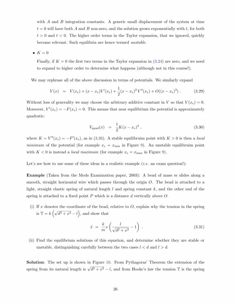
Let’s see how to use some of these ideas in a realistic example (i.e. an exam question!):
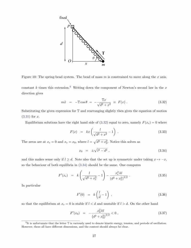
Example (Taken from the Mods Examination paper, 2003): A bead of mass m slides along a
smooth, straight horizontal wire which passes through the origin O. The bead is attached to a
light, straight elastic spring of natural length l and spring constant k, and the other end of the
spring is attached to a fixed point P which is a distance d vertically above O.
(i) If x denotes the coordinate of the bead, relative to O, explain why the tension in the spring
is T = k(√
d2 + x2 − l)
, and show that
x =k
mx
(l√
d2 + x2− 1
). (3.31)
(ii) Find the equilibrium solutions of this equation, and determine whether they are stable or
unstable, distinguishing carefully between the two cases l < d and l > d.
Solution: The set up is shown in Figure 10. From Pythagoras’ Theorem the extension of the
spring from its natural length is√d2 + x2 − l, and from Hooke’s law the tension T is the spring
26
d
fixed
x
T
O
P
θ
m
Figure 10: The spring-bead system. The bead of mass m is constrained to move along the x axis.
constant k times this extension.9 Writing down the component of Newton’s second law in the x
direction gives
mx = −T cos θ = − Tx√d2 + x2
≡ F (x) . (3.32)
Substituting the given expression for T and rearranging slightly then gives the equation of motion
(3.31) for x.
Equilibrium solutions have the right hand side of (3.32) equal to zero, namely F (xe) = 0 where
F (x) = kx
(l√
d2 + x2− 1
). (3.33)
The zeros are at xe = 0 and xe = x0, where l =√d2 + x2
0. Notice this solves as
x0 = ±√l2 − d2 , (3.34)
and this makes sense only if l ≥ d. Note also that the set up is symmetric under taking x 7→ −x,
so the behaviour of both equilibria in (3.34) should be the same. One computes
F ′(xe) = k
(l√
d2 + x2e
− 1
)− x2
e kl
(d2 + x2e)
3/2. (3.35)
In particular
F ′(0) = k
(l
d− 1
), (3.36)
so that the equilibrium at xe = 0 is stable if l < d and unstable if l > d. On the other hand
F ′(x0) = − x20 kl(
d2 + x20
)3/2 < 0 , (3.37)
9It is unfortunate that the letter T is variously used to denote kinetic energy, tension, and periods of oscillation.However, these all have different dimensions, and the context should always be clear.
27
implying that x0 only exists as a distinct equilibrium when l > d, and in this case it is stable. �
Remark: You might ask: what about the component of Newton’s second law in the vertical
direction? In particular, what balances the vertical force T sin θ to constrain the bead to move
only along the x axis? This is an example of a constraint force, studied in detail in section 5.
Revisit this example after we cover that section, and ask yourself these questions again!
3.4 * Damped motion
This subsection is starred: the material is not explicitly on the syllabus, and we are unlikely to have
time to cover it in lectures. However, the discussion naturally follows on from that in the previous
subsection, the equations of motion may be solved explicitly, and the dynamics is interesting.
We’ve seen that any system near stable equilibrium is described by simple harmonic motion.
More realistically, in practical applications there will be energy loss; or, as we’ve already com-
mented, more accurately mechanical energy will be converted to other forms of energy (typically
heat), that is not apparent in our description of the system. To model this we must assume that
the force F = F (x, x) depends on both position x and velocity x. For small displacements we may
treat both of these as small, neglecting the quadratic terms x2, xx, x2, and higher order terms in
a Taylor expansion. This leads to the damped harmonic oscillator, with force
F = −kx− b x . (3.38)
We assume that b > 0 and k > 0, so that the term −b x damps the motion (see the discussion after
(3.15)) of a stable equilibrium point (hence k > 0) at x = 0. Newton’s second law is
mx+ b x+ kx = 0 . (3.39)
We seek solutions of the form x(t) = ept. Substituting this into (3.39) gives the quadratic equation
mp2 + bp+ k = 0 , (3.40)
which has roots
p = −γ ±√γ2 − ω2
0 . (3.41)
Here we have defined the new parameters
γ =b
2m, ω0 =
√k
m= frequency of undamped oscillator . (3.42)
There are three cases:
Large damping
For large b, so that γ > ω0, both roots in (3.41) are real and negative:
p = −γ± , where γ± = γ ±√γ2 − ω2
0 > 0 . (3.43)
28
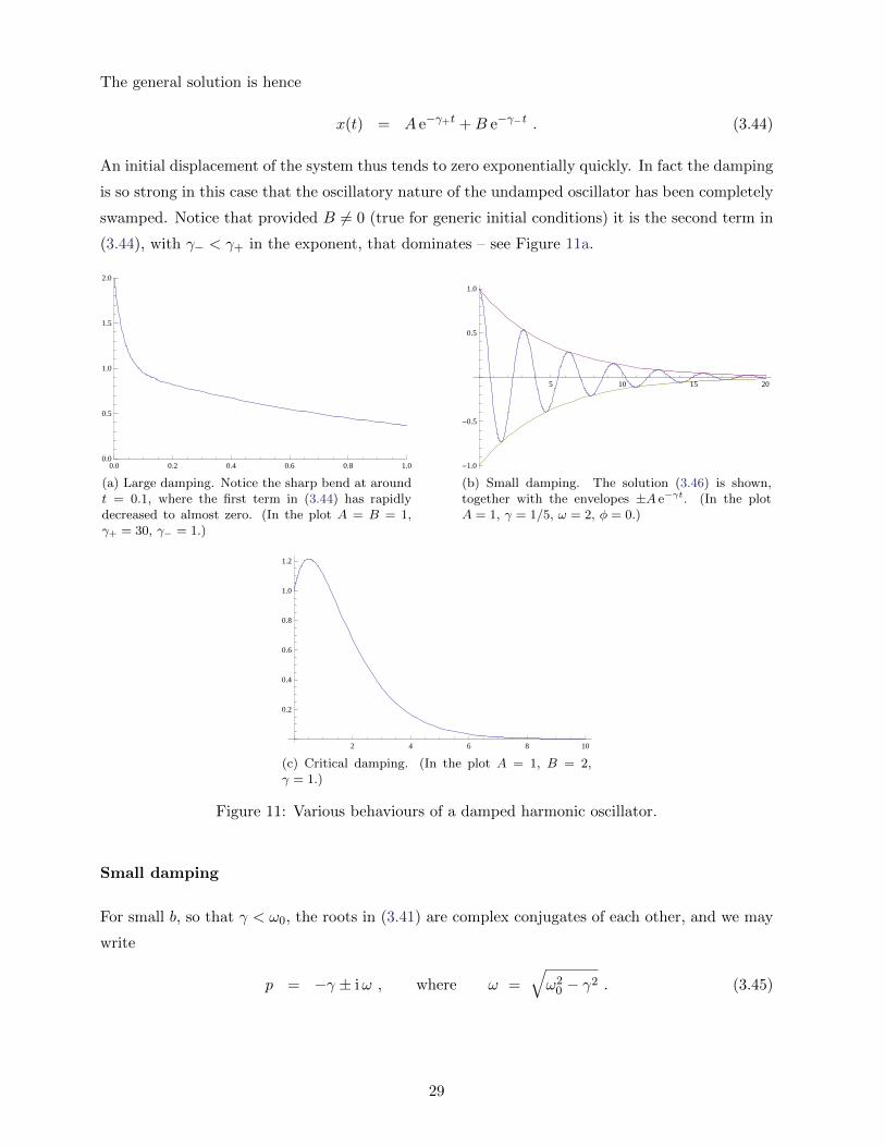
The general solution is hence
x(t) = A e−γ+t +B e−γ−t . (3.44)
An initial displacement of the system thus tends to zero exponentially quickly. In fact the damping
is so strong in this case that the oscillatory nature of the undamped oscillator has been completely
swamped. Notice that provided B 6= 0 (true for generic initial conditions) it is the second term in
(3.44), with γ− < γ+ in the exponent, that dominates – see Figure 11a.
0.0 0.2 0.4 0.6 0.8 1.00.0
0.5
1.0
1.5
2.0
(a) Large damping. Notice the sharp bend at aroundt = 0.1, where the first term in (3.44) has rapidlydecreased to almost zero. (In the plot A = B = 1,γ+ = 30, γ− = 1.)
5 10 15 20
-1.0
-0.5
0.5
1.0
(b) Small damping. The solution (3.46) is shown,together with the envelopes ±A e−γt. (In the plotA = 1, γ = 1/5, ω = 2, φ = 0.)
2 4 6 8 10
0.2
0.4
0.6
0.8
1.0
1.2
(c) Critical damping. (In the plot A = 1, B = 2,γ = 1.)
Figure 11: Various behaviours of a damped harmonic oscillator.
Small damping
For small b, so that γ < ω0, the roots in (3.41) are complex conjugates of each other, and we may
write
p = −γ ± iω , where ω =√ω2
0 − γ2 . (3.45)
29
This gives
x(t) =1
2α e−γt+iωt +
1
2β e−γt−iωt = Re
[α e−γt+iωt
]= A e−γt cos (ωt+ φ) , (3.46)
where the relation between the integration constants in the different forms of the solution are
α = A eiφ, β = A e−iφ. The solution hence oscillates with angular frequency ω < ω0, but with
exponentially decreasing amplitude Ae−γt – see Figure 11b.
Notice that there are two characteristic timescales for the damped oscillator:
• The period of the undamped oscillator, T0 =2π
ω0= 2π
√m
k.
• The decay time TD =1
γ=
2m
b, which by definition is the time it takes for the amplitude to
decay from its initial value by a factor of 1/e.
We may hence form a dimensionless parameter
Q =2πTDT0
=ω0
γ= 2
√km
b2. (3.47)
This is called the quality factor of the damped oscillator. Q > 1 and Q < 1 are small and large
damping, respectively, while Q = 1 is called critical damping.
Critical damping
When γ = ω0 the two roots of p in (3.41) coincide, giving only one solution to the original
ODE (3.39). The “missing” solution is easily checked to be x = t e−γt, giving the general solution
x(t) = (A+B t) e−γt . (3.48)
As for large damping, there are no oscillations – see Figure 11c. Many systems are engineered to
be critically damped, e.g. the suspension in a car. To see why, suppose that all the parameters
in the damped oscillator are fixed, apart from the friction coefficient b (or equivalently γ given
by (3.42)), that we are free to adjust. Then by tuning γ = ω0, we ensure that a generic small
displacement of the corresponding critically damped system decays more rapidly than for the same
system with large damping (since the exponent γ = ω0 > γ−, where recall that the γ− mode in
(3.44) dominates). In addition, the system just fails to oscillate. Thus if we want to damp out
general oscillations of a system as quickly as possible, we should tune it to be critically damped.
3.5 Coupled oscillations
So far in this section we have only considered systems with one degree of freedom, i.e. where the
motion is described by a single function x(t). In this section we briefly consider the stability of
30
systems with two degrees of freedom. The general case is described, using more powerful methods,
in the course B7.1 Classical Mechanics.
Suppose we have a dynamical system described by the coupled ODEs
x = F (x, y) , y = G(x, y) , (3.49)
where we shall assume that F and G are suitably analytic.10 As in section 3.3, an equilibrium
configuration is a solution to (3.49) with x = xe, y = ye both constant. Thus F (xe, ye) = 0 =
G(xe, ye). To determine the stability of such an equilibrium point, we again linearize the equations
of motion. This means that we write
x = xe + ξ , y = ye + η , (3.50)
where ξ and η are small, and then Taylor expand the right hand sides of (3.49), leading to
ξ = F (xe + ξ, ye + η) = F (xe, ye) + ξ∂F
∂x(xe, ye) + η
∂F
∂y(xe, ye) + · · · ,
η = G(xe + ξ, ye + η) = G(xe, ye) + ξ∂G
∂x(xe, ye) + η
∂G
∂y(xe, ye) + · · · , (3.51)
where · · · denote terms of quadratic and higher order in ξ, η. The linearized equations of motion
are hence
ξ = a ξ + b η ,
η = c ξ + d η , (3.52)
where we have introduced the constants
a =∂F
∂x(xe, ye) , b =
∂F
∂y(xe, ye) ,
c =∂G
∂x(xe, ye) , d =
∂G
∂y(xe, ye) . (3.53)
One could potentially try to solve (3.52) by e.g. solving the first equation for η in terms of ξ
(assuming b 6= 0), and substituting into the second equation: this gives a fourth order ODE in ξ.
However, it is better to write (3.52) as a matrix equation(ξ
η
)=
(a b
c d
)(ξ
η
). (3.54)
We then seek solutions to (3.54) of the form(ξ(t)
η(t)
)=
(α
β
)eλt , (3.55)
10Here x and y denote general variables, rather than Cartesian coordinates.
31
where α, β and λ are constant. Substituting (3.55) into (3.54) and cancelling the overall factor of
eλt gives
λ2
(α
β
)=
(a b
c d
)(α
β
). (3.56)
This says that λ2 is an eigenvalue of the matrix
(a b
c d
), with corresponding eigenvector
(α
β
).
The characteristic equation is
det
[λ2
(1 0
0 1
)−
(a b
c d
)]= λ4 − (a+ d)λ2 + (ad− bc) = 0 , (3.57)
which gives the eigenvalues
λ2 =1
2
(a+ d±
√(a+ d)2 − 4(ad− bc)
)≡ λ2
± . (3.58)
For a general system (3.49) the solutions for λ2 in (3.58) can be complex, in general also leading
to complex λ. Recall that the linearized solution (3.55) is proportional to eλt = eRe(λ)t · ei Im(λ)t.
The imaginary part of λ determines the oscillatory part of the solution, while the real part of λ
determines the time-dependent amplitude.11 Notice that we may take either sign for the square
root in solving (3.58) for λ, implying in general 4 solutions ±λ±. This is the number we expect
for two coupled second order ODEs (3.49). Let’s look at a simple example.
Example: Consider two particles, each of massm, attached to three springs, as shown in Figure 12.
The springs have equilibrium length l and spring constants k, and lie on a line. One end of the
first spring is fixed, while the other end is attached to a particle of mass m. This mass is in turn
attached to one end of the second spring, with the other end attached to a second particle of mass
m. Finally, this second mass is attached to one end of the third spring, with the other end fixed.
We denote the horizontal displacement of the first mass from its equilibrium position by x, and
similarly the horizontal displacement of the second mass by y.
By Hooke’s law the forces shown in Figure 12 are (careful with signs!)
F1 = kx , F2 = k(y − x) , F3 = −ky . (3.59)
Applying Newton’s second law for each particle thus gives
mx = F2 − F1 = k(y − 2x) ,
my = F3 − F2 = k(x− 2y) . (3.60)
Comparing to the general formulae (3.49), (3.52) we see that the equations are already linear, and
that there is one equilibrium point at x = y = 0. Thus in this case we may identify x = ξ, y = η.
11* If you read section 3.4, compare/contrast this with the discussion of the damped oscillator around equation(3.40).
32

l
fixed
l l
m mfixed
x y
F3F2F2F1
Figure 12: The system of masses and springs. The upper diagram shows the equilibrium config-uration. In the lower diagram we have shown the horizontal displacements x and y of the twomasses from their equilibrium positions, together with the various Hooke’s law forces F1, F2, F3
acting.
In matrix form (3.60) reads (x
y
)=
(−2km
km
km −2k
m
)(x
y
). (3.61)
Comparing to (3.54) we read off
a = d = −2k
m, b = c =
k
m, (3.62)
and hence from (3.58) that
λ2 =k
2m(−4± 2) =⇒ λ = ±i
√k
m, ±i
√3k
m. (3.63)
Since the linearized modes (3.55) are proportional to eλt, and in this case all λ are purely imaginary,
the corresponding solutions are hence oscillatory. The two values of λ2 in (3.63) correspond to the
two eigenvectors (1,±1)T of the matrix in (3.61), respectively. �
Returning to the general case, this motivates the following definition:
Definition If all solutions for λ = ±λ± given by (3.58) are purely imaginary (equivalently both
λ2± < 0), we say the equilibrium point is stable. We write λ = ±iω±, where ω± > 0 are called the
normal frequencies of the system. Writing eλt = e±iω±t in terms of trigonometric functions, the
linearized solution is(ξ(t)
η(t)
)=
(α+
β+
)cos (ω+t+ φ+) +
(α−
β−
)cos (ω−t+ φ−) , (3.64)
where
(α±
β±
)are the eigenvectors corresponding to the eigenvalues λ2
±, respectively, and φ± are
constants. The solution for a given eigenvector is called a normal mode.
33
Example: For the system of masses and springs, the normal frequencies are ω+ =√k/m, ω− =√
3k/m. The general solution is hence(x(t)
y(t)
)=
(1
1
)A cos
(√k
mt+ φ
)+
(1
−1
)B cos
(√3k
mt+ θ
), (3.65)
where A, B, φ and θ are constants. The lower frequency ω+ normal mode has the two masses
oscillating together, while the higher frequency ω− normal mode has the two masses oscillating in
opposite directions. �
The essential point of (3.64) is that near a stable equilibrium point the system behaves like two
independent one-dimensional harmonic oscillators, of frequencies ω±. By solving for the eigenvalues
and eigenvectors of the matrix in (3.54) we have essentially diagonalized the motion, with each
normal mode being simple harmonic motion. A general perturbation (3.64) of the system is a
linear combination of these two modes.
Finally, notice that if any eigenvalue λ has a non-zero real part there will be an exponentially
growing mode, with amplitude proportional to eRe(λ) t with Re(λ) > 0, and the equilibrium point
will be unstable.
34
4 Motion in higher dimensions
In this section we develop some general formalism that is useful for analysing dynamics in two
and three dimensions. In particular in sections 4.2 and 4.3 we introduce conservative forces and
central forces, respectively. The dynamics for each of these forces leads to a conserved quantity,
i.e. a quantity that is constant during the motion. Conserved quantities are very important in
dynamics: by definition one has at least partially integrated the equations of motion whenever one
finds a conserved quantity. Conservative forces and central forces lead to conservation of energy
and angular momentum, respectively. In this section we focus on developing the theory, with a
few very simple examples, but then apply this to more sophisticated examples in sections 5 and 6.
4.1 Planar motion in polar coordinates
Motion in a plane is sometimes conveniently described using polar coordinates. Recall that Carte-
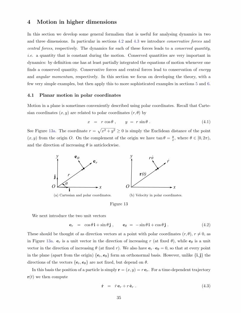
sian coordinates (x, y) are related to polar coordinates (r, θ) by
x = r cos θ , y = r sin θ . (4.1)
See Figure 13a. The coordinate r =√x2 + y2 ≥ 0 is simply the Euclidean distance of the point
(x, y) from the origin O. On the complement of the origin we have tan θ = yx , where θ ∈ [0, 2π),
and the direction of increasing θ is anticlockwise.
y
O x
r
θ
ereθ
i
j
(a) Cartesian and polar coordinates.
y
O x
r
θ
(t)
rr
(b) Velocity in polar coordinates.
Figure 13
We next introduce the two unit vectors
er = cos θ i + sin θ j , eθ = − sin θ i + cos θ j . (4.2)
These should be thought of as direction vectors at a point with polar coordinates (r, θ), r 6= 0, as
in Figure 13a. er is a unit vector in the direction of increasing r (at fixed θ), while eθ is a unit
vector in the direction of increasing θ (at fixed r). We also have er · eθ = 0, so that at every point
in the plane (apart from the origin) {er, eθ} form an orthonormal basis. However, unlike {i, j} the
directions of the vectors {er, eθ} are not fixed, but depend on θ.
In this basis the position of a particle is simply r = (x, y) = r er. For a time-dependent trajectory
r(t) we then compute
r = r er + r er . (4.3)
35
But from (4.2) we have
er = −θ sin θ i + θ cos θ j = θ eθ ,
eθ = −θ cos θ i− θ sin θ j = −θ er , (4.4)
and hence
r = r er + rθ eθ . (4.5)
The second term has arisen because the basis we used is itself time-dependent, specifically due to
the time-dependence of θ = θ(t). The quantity θ is called the angular velocity. Equation (4.5)
expresses velocity r in polar coordinates – see Figure 13b. We may find a similar expression for
acceleration by taking another time derivative, using (4.4):
r = r er + r er + rθ eθ + rθ eθ + rθ eθ ,
= (r − rθ2) er + (2rθ + rθ) eθ ,
= (r − rθ2) er +1
r
d
dt(r2θ) eθ , (4.6)
Here in the last line we’ve written 2rθ + rθ = 1r
ddt(r
2θ).
Example (Uniform circular motion): Consider a particle moving in a circle of radius R, centre the
origin, at constant speed v. Since r = R = constant we have r = 0. Thus from (4.5) its velocity is
r = R θ eθ . (4.7)
This is tangent to the circle. The particle’s speed is v = |r|, which implies v = R|θ|, and hence
the angular speed |θ| = vR is constant. Since θ is constant, θ = 0, and similarly since r = 0 we also
have r = 0. Thus from (4.6) the acceleration is
r = −R θ2 er = −v2
Rer . (4.8)
We conclude that the acceleration in uniform circular motion has magnitude v2/R, and is directed
towards the centre of the circle O. Newton’s second law implies that in order to generate this
acceleration we need a force of magnitude F = mv2/R = mR θ2 directed towards the origin – this
is called the centripetal force. �
4.2 Conservative forces
In section 3.1 we saw that for motion in one dimension and forces F = F (x) there is a conserved
energy. In three dimensions this is no longer necessarily the case: we need an additional constraint
on F = F(r) in order for energy to be conserved. Even before looking at the details one might have
anticipated this: energy is a scalar quantity, and without any further input there is no natural way
to construct a scalar from the vector F, analogously to what we did in one dimension.
36

Definition The kinetic energy of a particle is T = 12m|r|
2, where r(t) is the particle’s position in
an inertial frame.
We then have the following important result:
Conservation of Energy Theorem The quantity
E = T + V =1
2m|r|2 + V (r) , (4.9)
is conserved if the force F = F(r) takes the form
F = −∇V . (4.10)
That is, in Cartesian coordinates F = (−∂xV,−∂yV,−∂zV ).
Proof: Suppose that the force takes the form (4.10). Using the chain rule we compute
E = mr · r +∇V · r
= (mr− F) · r = 0 , (4.11)
where the last step uses Newton’s second law. �
To understand where the condition (4.10) really comes from, it is useful to first generalize the
notion of work to three dimensions:
Definition The work done by a force F in moving a particle from r1 to r2 along a curve C is
W =
∫C
F · dr . (4.12)
The distinction with the corresponding definition in one dimension (3.4) is that in higher dimen-
sions the line integral (4.12) depends on the precise curve C, and not just on its endpoints r1, r2.
If we now suppose that r(t) is the trajectory of a particle satisfying Newton’s second law, starting
at position r1 = r(t1) and ending at r2 = r(t2), then we may write
W =
∫ t2
t1
F · r dt = m
∫ t2
t1
r · r dt =1
2m
∫ t2
t1
d
dt|r|2 dt = T (t2)− T (t1) . (4.13)
Thus, as in one dimension, the work done by the force is the change in kinetic energy.
Suppose now that the total energy E given by (4.9) is conserved. This means that E = T (t1) +
V (r1) = T (t2) + V (r2), and hence (4.13) implies that
W =
∫C
F · dr = V (r1)− V (r2) . (4.14)
The right hand side manifestly depends only on the endpoints r1, r2 of the curve C, and we have
thus shown that if energy is conserved then the work done is independent of the choice of curve C
37
connecting r1 to r2. In the Prelims Multivariable Calculus course you prove that if this is true for
all curves C then F takes the form (4.10).12
Definition A force F = F(r) is said to be conservative if there exists a potential energy function
V = V (r) such that
F = −∇V . (4.15)
Note that as in one dimension the potential V is only defined up to an additive constant.
Examples:
(i) Any constant force Fconst is conservative, with potential V (r) = −Fconst · r. An important
example is gravity: for F = −mg k the corresponding potential function is simply V (r) =
mg k · r = mgz.
(ii) In section 6.1 we’ll show that any force of the form F = F (|r|) er is conservative, where
er = r/|r|. These also play a particularly important role in Dynamics.
Conservative forces enjoy the following equivalent definitions:
Theorem (From Prelims Multivariable Calculus) Let F : S → R3 be a vector field, where the
domain S ⊂ R3 is open and path connected. Then the following three statements are equivalent:
1. F is conservative, i.e. there exists a potential V : S → R such that F = −∇V .
2. Given any two points r1, r2 in S, and any curve C in S starting at r1 and ending at r2, then
the integral∫C F · dr is independent of the choice of C.
3. For any simple closed curve C in S we have∫C F · dr = 0.
It is also shown in Multivariable Calculus that conservative forces satisfy ∇∧F = 0, although we
won’t need this fact.
4.3 Central forces and angular momentum
Another important concept is that of a central force:
Definition A force that is always directed along the line joining a particle to a fixed position in
an inertial frame is called a central force. It is usually convenient to choose this point as the origin
of the frame, meaning that
F ∝ r , (4.16)
where r is the position vector of the particle, measured from the origin O.
12See the Theorem below. Note also that if F takes the form (4.10), the second equality in (4.14) is just theFundamental Theorem of Calculus.
38
The importance of central forces is that they always lead to an associated conserved vector quantity.
Definition The angular momentum L = LP of a particle about a point P in an inertial frame is
the moment of linear momentum p = mr about P . That is,
LP ≡ (r− x) ∧mr = (r− x) ∧ p . (4.17)
Here x is the position vector of the point P , while r is the position of the particle (both measured
from the origin O). Notice that r is the velocity of the particle in the inertial frame, not the
velocity relative to P (which could in principle be moving, x = x(t)).
This definition makes it clear that the angular momentum depends on the point P . However, for
central forces there is a natural choice for P , namely P = O, the centre of the force.
Proposition If a particle is acted on by a central force with centre O then the angular momentum
L = LO is conserved, and the path of the particle lies entirely in a fixed plane through O. That
is, the motion is planar.
Proof: We compute
L =d
dt(r ∧mr) = r ∧mr + r ∧mr = r ∧mr . (4.18)
The last equality follows since a ∧ a = 0 for any vector a. Newton’s second law then gives
L = r ∧mr = r ∧ F = 0 , (4.19)
where the last equality follows since F ∝ r for a central force. Thus L is constant. In the special
case that L = r ∧mr = 0 the position and velocity must be parallel (a ∧ b = 0 implies a and b
are parallel, where we include this to mean that one or both are zero). Thus the particle either
moves in a straight line through the origin, or in the special case that r = 0 sits at a fixed point.
More generally if L 6= 0 then notice that L · r = 0 = L · r both follow from L = r ∧mr, meaning
that L is always perpendicular to both the position of the particle and its velocity. This means
that the motion is confined to the plane through O with normal vector L – see Figure 14. �
Suppose that L = LO is conserved, as in the last Proposition. In particular the direction of
L is constant, and we may choose this as the z direction, so that LO ∝ k. Introducing polar
coordinates for the planar motion in the (x, y) plane, we compute
L = r ∧mr = r er ∧m(r er + rθ eθ
),
= mr2θ k , (4.20)
where we have used (4.5) in the first line, and k = i ∧ j = er ∧ eθ in the last step. This proves the
following result, which will be important later:
39
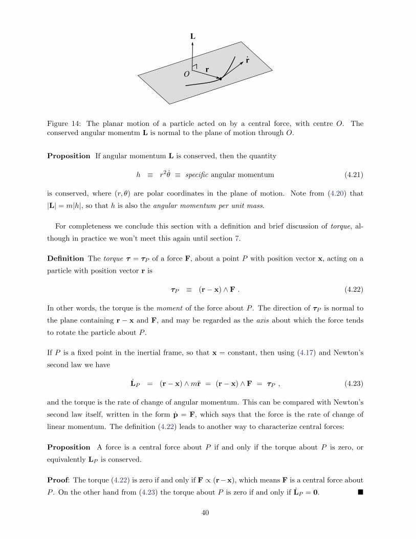
rO
L
r
Figure 14: The planar motion of a particle acted on by a central force, with centre O. Theconserved angular momentm L is normal to the plane of motion through O.
Proposition If angular momentum L is conserved, then the quantity
h ≡ r2θ ≡ specific angular momentum (4.21)
is conserved, where (r, θ) are polar coordinates in the plane of motion. Note from (4.20) that
|L| = m|h|, so that h is also the angular momentum per unit mass.
For completeness we conclude this section with a definition and brief discussion of torque, al-
though in practice we won’t meet this again until section 7.
Definition The torque τ = τP of a force F, about a point P with position vector x, acting on a
particle with position vector r is
τP ≡ (r− x) ∧ F . (4.22)
In other words, the torque is the moment of the force about P . The direction of τP is normal to
the plane containing r − x and F, and may be regarded as the axis about which the force tends
to rotate the particle about P .
If P is a fixed point in the inertial frame, so that x = constant, then using (4.17) and Newton’s
second law we have
LP = (r− x) ∧mr = (r− x) ∧ F = τP , (4.23)
and the torque is the rate of change of angular momentum. This can be compared with Newton’s
second law itself, written in the form p = F, which says that the force is the rate of change of
linear momentum. The definition (4.22) leads to another way to characterize central forces:
Proposition A force is a central force about P if and only if the torque about P is zero, or
equivalently LP is conserved.
Proof: The torque (4.22) is zero if and only if F ∝ (r−x), which means F is a central force about
P . On the other hand from (4.23) the torque about P is zero if and only if LP = 0. �
40
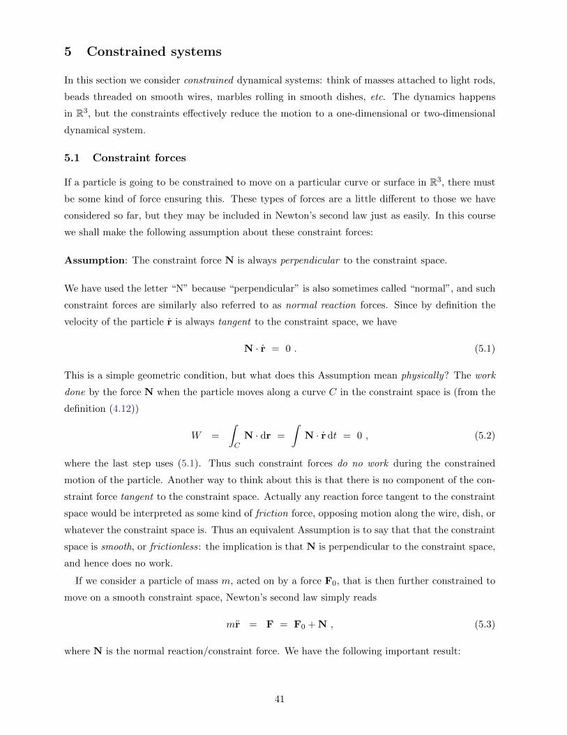
5 Constrained systems
In this section we consider constrained dynamical systems: think of masses attached to light rods,
beads threaded on smooth wires, marbles rolling in smooth dishes, etc. The dynamics happens
in R3, but the constraints effectively reduce the motion to a one-dimensional or two-dimensional
dynamical system.
5.1 Constraint forces
If a particle is going to be constrained to move on a particular curve or surface in R3, there must
be some kind of force ensuring this. These types of forces are a little different to those we have
considered so far, but they may be included in Newton’s second law just as easily. In this course
we shall make the following assumption about these constraint forces:
Assumption: The constraint force N is always perpendicular to the constraint space.
We have used the letter “N” because “perpendicular” is also sometimes called “normal”, and such
constraint forces are similarly also referred to as normal reaction forces. Since by definition the
velocity of the particle r is always tangent to the constraint space, we have
N · r = 0 . (5.1)
This is a simple geometric condition, but what does this Assumption mean physically? The work
done by the force N when the particle moves along a curve C in the constraint space is (from the
definition (4.12))
W =
∫C
N · dr =
∫N · r dt = 0 , (5.2)
where the last step uses (5.1). Thus such constraint forces do no work during the constrained
motion of the particle. Another way to think about this is that there is no component of the con-
straint force tangent to the constraint space. Actually any reaction force tangent to the constraint
space would be interpreted as some kind of friction force, opposing motion along the wire, dish, or
whatever the constraint space is. Thus an equivalent Assumption is to say that that the constraint
space is smooth, or frictionless: the implication is that N is perpendicular to the constraint space,
and hence does no work.
If we consider a particle of mass m, acted on by a force F0, that is then further constrained to
move on a smooth constraint space, Newton’s second law simply reads
mr = F = F0 + N , (5.3)
where N is the normal reaction/constraint force. We have the following important result:
41
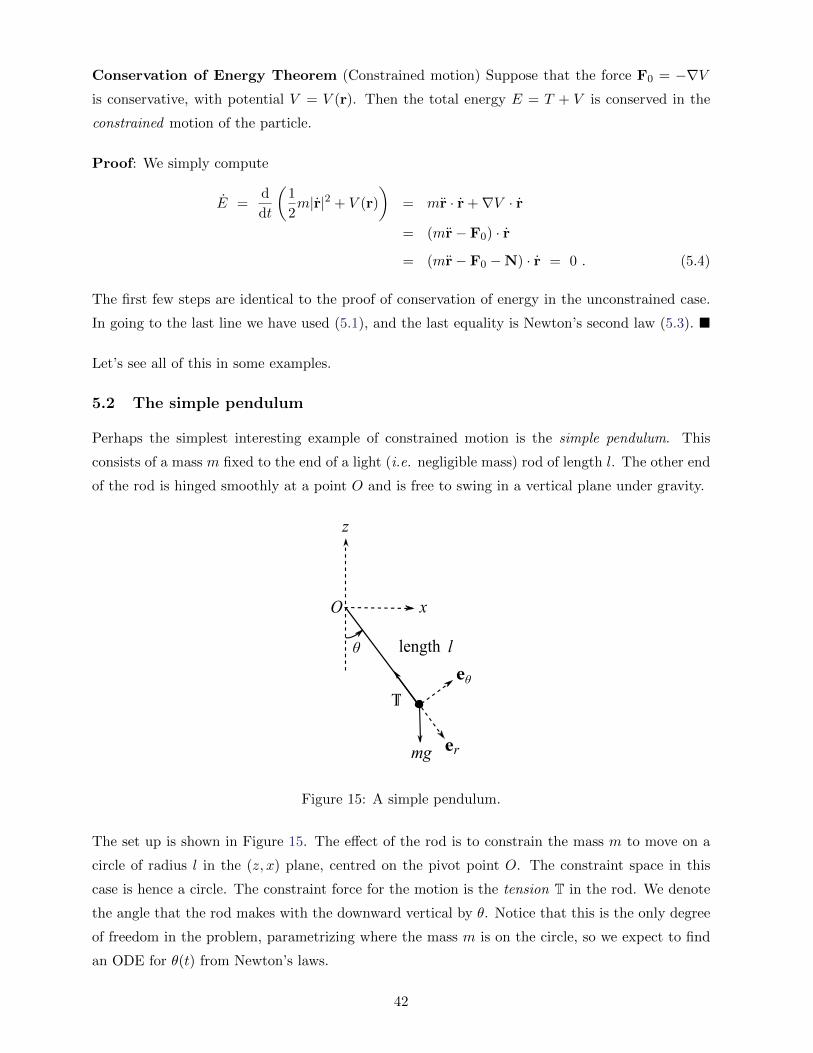
Conservation of Energy Theorem (Constrained motion) Suppose that the force F0 = −∇Vis conservative, with potential V = V (r). Then the total energy E = T + V is conserved in the
constrained motion of the particle.
Proof: We simply compute
E =d
dt
(1
2m|r|2 + V (r)
)= mr · r +∇V · r
= (mr− F0) · r
= (mr− F0 −N) · r = 0 . (5.4)
The first few steps are identical to the proof of conservation of energy in the unconstrained case.
In going to the last line we have used (5.1), and the last equality is Newton’s second law (5.3). �
Let’s see all of this in some examples.
5.2 The simple pendulum
Perhaps the simplest interesting example of constrained motion is the simple pendulum. This
consists of a mass m fixed to the end of a light (i.e. negligible mass) rod of length l. The other end
of the rod is hinged smoothly at a point O and is free to swing in a vertical plane under gravity.
x
T
z
O
mg
θ
er
eθ
length l
Figure 15: A simple pendulum.
The set up is shown in Figure 15. The effect of the rod is to constrain the mass m to move on a
circle of radius l in the (z, x) plane, centred on the pivot point O. The constraint space in this
case is hence a circle. The constraint force for the motion is the tension T in the rod. We denote
the angle that the rod makes with the downward vertical by θ. Notice that this is the only degree
of freedom in the problem, parametrizing where the mass m is on the circle, so we expect to find
an ODE for θ(t) from Newton’s laws.
42

Given that the motion will lie on a circle, it is useful to introduce polar coordinates in the (z, x)
plane: z = −l cos θ, x = l sin θ. The corresponding unit vectors are
er = − cos θ k + sin θ i , eθ = sin θ k + cos θ i . (5.5)
See Figure 15. Although these are slightly different to the polar coordinates in the (x, y) plane in
Figure 13a, the essential point is that as in (4.4) we again have er = θ eθ, eθ = −θ er. It follows
that the velocity and acceleration are again given by (4.5) and (4.6), respectively, where r = (z, x).
The forces acting on the mass m are gravity and the constraint force: in the notation of sec-
tion 5.1 we have
F0 = −mg k , N = −T er , (5.6)
where the total force acting is F = F0 + N. Notice in particular that the constraint force N acts
in the radial direction, and is thus always perpendicular to the constrained motion in a circle: this
follows from our general discussion in section 5.1, and the fact that the rod is “hinged smoothly”
at O.
Newton’s second law (5.3) is a vector equation, and we may conveniently pick out different
components of it by taking dot products with the linearly independent vectors er, eθ. Since
k = − cos θ er + sin θ eθ, taking the dot product of Newton’s second law (5.3) with eθ gives
mr · eθ = F · eθ = −mg sin θ . (5.7)
From (4.6) we have r · eθ = 2rθ + rθ. However, here r = l is constant, so that (5.7) reads
mlθ = −mg sin θ, which rearranges to
θ = −gl
sin θ . (5.8)
This is the equation of motion for the simple pendulum: a second order ODE for θ(t). Of course,
this is only “half” of Newton’s second law. To obtain the remaining equation we take the dot
product of (5.3) with er:
mr · er = F · er = mg cos θ − T . (5.9)
On the other hand from (4.6) we have r · er = r − rθ2 = −lθ2. Thus (5.9) rearranges to
T = mlθ2 +mg cos θ . (5.10)
This says that the tension T balances the component of the weight along the rod mg cos θ, and the
centripetal force mlθ2 for circular motion about the origin O.
We cannot solve the equation of motion (5.8) in closed form, as simple as it looks. However, we
have our dynamics toolbox to apply: let’s look at the equilibrium configurations, and conservation
of energy.
43
Equilibria: Notice there are two equilibrium configurations, where the right hand side of (5.8)
is zero: θ = 0 and θ = π. The former has the pendulum hanging down vertically, and for small
oscillations (i.e. small θ) we may approximate sin θ ' θ. In this linearized approximation (5.8)
becomes
θ = −ω2θ , where ω2 =g
l> 0 . (5.11)
Thus, as is intuitively obvious, θ = 0 is a stable equilibrium, in the terminology of section 3.3. For
small oscillations about this point the pendulum executes simple harmonic motion with angular
frequency ω, and hence period
T = 2π
√l
g. (5.12)
Notice that√l/g indeed has dimensions of time, and that in fact this is the only way we can
construct such a quantity from the variables in the problem. Thus T had to be a dimensionless
number times√l/g.
The second equilibrium position, θ = π, has the rod precariously balanced above the pivot point
O. Setting θ = π+ξ(t), with ξ(t) small, we may now approximate sin θ = sin(π+ξ) ' − sin ξ ' −ξ.The linearized equation of motion obtained from (5.8) thus reads
ξ = −gl(−ξ) =
g
lξ . (5.13)
The general solution is ξ(t) = C e√g/l t +D e−
√g/l t, and the equilibrium is unstable.
Conservation of energy: The Conservation of Energy Theorem at the end of section 5.1 guar-
antees that the total energy of the mass is conserved: the gravitational force F0 = −mg k is
conservative, with potential V (r) = V (x, y, z) = mgz. The total energy is
E =1
2m|r|2 + V (r) =
1
2ml2θ2 −mgl cos θ . (5.14)
Here in the second equality we have substituted r = lθ eθ for circular motion, and z = −l cos θ.
Let’s check explicitly that E is indeed conserved:
E = ml2θθ +mgl sin θ θ = ml2θ(θ +
g
lsin θ
). (5.15)
We thus see that E = 0, provided the equation of motion (5.8) holds.
As in section 3.2, we may view (5.14) as a first order ODE for θ(t), and integrate it. Rerranging
we have
θ2 =2E
ml2+
2g
lcos θ , (5.16)
which integrates to
t = ±∫
dθ√2E/ml2 + 2(g/l) cos θ
. (5.17)
44

If we assume that the pendulum starts at θ = 0 at time t = 0, and reaches a maximum angle of
θ0 > 0 in its swing, then we may compute the period of the swing:
T = 4
∫ θ0
0
dθ√2E/ml2 + 2(g/l) cos θ
= 4
√l
g
∫ θ0
0
dθ√2 cos θ − 2 cos θ0
. (5.18)
Here we have noted that at the top of the swing θ = 0, and hence from (5.16) cos θ0 = −E/mgl. The
factor of 4 in (5.18) arises because the integral from 0 to θ0 is only a quarter of one period. Compare
to the result for small oscillations (5.12). One can derive this from the general formula (5.18) by
making the approximation cos θ ' 1− 12θ
2 in the integral. More generally the integral in (5.18) is
an elliptic integral. We also see that the period T is a dimensionless number times√l/g, where
the dimensionless number in general depends on the initial conditions (via the conserved energy
E).
Finally, notice that we have tacitly assumed that |E| ≤ mgl in the above discussion. From
(5.14) we have E ≥ −mgl, with equality for the stable equilibrium at θ = 0. However, if E > mgl
then cos θ0 = −E/mgl has no solution, and hence θ is never zero. In this case the system has so
much energy that the pendulum swings over the top of the pivot point.
5.3 Motion on a surface under gravity
Consider a mass m moving under gravity on a smooth surface. For example, this might model a
marble rolling in a dish, or a bicycle freewheeling down a hill. The gravitational force is, as usual,
F0 = −mg k, and this is conservative with potential V (r) = mgz. The fact that the surface is
smooth means that the constraint force is perpendicular to the surface.
Mathematically, there are different ways in which we can specify a surface in R3 (see the last part
of the Geometry course). For example, we can define a surface as the zero set of some suitable
function f : R3 → R. A normal vector to the surface is ∇f , and the constraint force will be
proportional to this. Rather than trying to describe the general situation, here we’ll focus on a
surface of revolution. This may be specified as
f(r, θ, z) ≡ z −H(r) = 0 , (5.19)
where (r, θ, z) are cylindrical polar coordinates. Recall this means that the Cartesian (x, y) coor-
dinates are given by x = r cos θ, y = r sin θ. The defining equation (5.19) specifies the height z
as a function z = H(r) of the radial distance r in the (x, y) plane – see Figure 16. Since this
is independent of θ the resulting surface will be invariant under rotation about the z axis, which
rotates the θ coordinate. This also implies that eθ is tangent to the surface at every point, and
hence in particular we have N · eθ = 0.
The position vector of the particle moving on the surface is
r = r er + z ez , (5.20)
45

O
mg
er
e
z
x
yθ
r
z = H(r)height
θ
ez
N
Figure 16: Particle moving under gravity on a surface of revolution.
where ez = k. Newton’s second law (5.3) thus reads
mr = F = −mg ez + N . (5.21)
Using (4.6) we may write the acceleration r in cylindrical polar coordinates, so that (5.21) reads
m
[(r − rθ2
)er +
1
r
d
dt
(r2θ)
eθ + z ez
]= −mg ez + N . (5.22)
Notice that every term in (5.22) is orthogonal to eθ, apart from the term proportional to eθ. Thus
we immediately deduce
1
r
d
dt
(r2θ)
= 0 =⇒ r2θ ≡ h = constant . (5.23)
From the general discussion in section 4.3 we see this has something to do with conservation of
angular momentum. However, in that section we also showed that the angular momentum LP
about a point P is conserved if and only if the force acting is a central force about P , i.e. the total
force F is always directed towards P . This clearly isn’t true in general for motion on a surface of
revolution. To see what’s going on, let us compute the angular momentum about the origin O:
L = LO = r ∧mr = m (r er + z ez) ∧(r er + rθ eθ + z ez
)= mr2θ ez +m(zr − rz) eθ −mzrθ er , (5.24)
where we have used er ∧ eθ = ez, eθ ∧ ez = er, ez ∧ er = eθ, which are easily checked from (4.2).
We thus have
L · ez = mr2θ = mh . (5.25)
46

We now see that (5.23) says that the component of angular momentum in the direction of the axis
of symmetry ez is conserved. In fact this is directly related to the rotational symmetry about this
axis, although an explanation of this will have to wait for the course B7.1 on Classical Mechanics.13
Let’s go back to Newton’s second law (5.22). This is a vector differential equation, and we have
so far taken the dot product with eθ to find the conserved quantity h in (5.23). There must be
two more scalar equations, and obviously we may obtain these by taking dot products with er and
ez. However, we should be a bit smarter and think about what we’re trying to do. The motion of
the particle is determined by finding r(t), θ(t) and z(t). Firstly, z(t) is fixed to be z(t) = H(r(t))
by the constraint (5.19). Secondly, the equation (5.23) determines θ = h/r2(t), which may be
integrated to find θ(t), once we know r(t). Thus at this stage we really only have one degree
of freedom in the problem, namely r(t). One linear combination of the remaining equations in
(5.22) should thus be an equation of motion for r(t). The other combination simply determines
the constraint force N, c.f. the simple pendulum, where equation (5.9) determined the tension in
the pendulum. If we want to obtain the equation of motion for r(t) directly, a nice geometric way
to do this is to take the dot product of (5.22) with another tangent vector to the surface: that way
N will immediately drop out. Since f(r, θ, z) = z −H(r) = 0 defines the surface, a normal vector
is14
n = ∇f = ez −H ′(r)er . (5.26)
The constraint force N is proportional to n. We have already used that eθ is tangent to the surface,
and from (5.26) another independent tangent vector is
t = H ′(r)ez + er . (5.27)
Clearly t·n = 0. Thus taking the dot product of Newton’s second law (5.22) with t gives (cancelling
an overall factor of the mass m)(r − rθ2
)+H ′(r) z = −g H ′(r) . (5.28)
On the other hand from (5.23) and the defining equation (5.19) we may substitute
θ =h
r2, z = H(r) , (5.29)
and from the chain rule
z = H ′(r) r , z = H ′′(r) r2 +H ′(r) r . (5.30)
Substituting these into (5.28) hence gives[1 +
(H ′(r)
)2]r +H ′(r)H ′′(r) r2 − h2
r3= −g H ′(r) . (5.31)
13** Noether’s Theorem, due to Emmy Noether, relates any continuous symmetry to a corresponding conservedquantity. In fact all the conserved quantities in this course arise in this way.
14The gradient in cylindrical polar coordinates is ∇f = ∂f∂r
er + 1r∂f∂θ
eθ + ∂f∂z
ez. See the Multivariable Calculuscourse.
47
This is a second order ODE for r(t), as we expected to find. Given H(r), in principle one can try
to solve this equation.
However, from the end of section 5.1 we also know that there is a conserved energy for this
problem. This will lead to a first order equation, and moreover the second order equation (5.31)
should be implied by this first order equation. Let’s see that this is indeed the case. From
conservation of energy we know that
E =1
2m|r|2 +mgz = constant . (5.32)
In cylindrical polars we compute
|r|2 = |r er + rθ eθ + z ez|2 = r2 + r2θ2 + z2 . (5.33)
Substituting using (5.29) into (5.32) we hence have
E =1
2m
[r2 +
h2
r2+(H ′(r)
)2r2
]+mgH(r) . (5.34)
Equation (5.34) is the expected first order ODE for r(t). It’s straightforward enough to take d/dt
of the right hand side of (5.34) and check (after cancelling an overall factor of r) this indeed gives
the equation (5.31). In the other direction, equation (5.34) may in principle be integrated, given
H(r), although typically one won’t be able to do the integral explicitly. Nevertheless, as we have
seen before one can often use conservation of energy to deduce various qualitative and quantitative
features of the motion. Let’s see this in a concrete example, with a specific choice of the surface
of revolution (i.e. choice of H(r)).
Example (Motion on a paraboloid): A particle moves under gravity on the smooth inside surface
of the paraboloid z = r2/4a. Initially it is at a height z = a and is projected horizontally with
speed v along the surface of the paraboloid. Show that the particle moves between two heights in
the subsequent motion, and find them.
Solution: We have H(r) = r2/4a. We begin by substituting the initial conditions into the
conserved specific angular momentum h = r2θ. At t = 0 we have z = a and hence since r2 = 4az
initially we have r = 2a. Moreover, since the particle is projected horizontally at speed v, in polar
coordinates (see Figure 13) we may identify r = 0, rθ = v initially. We thus compute
h = r2θ = r · rθ = 2av . (5.35)
Conservation of energy (5.32) reads
E =1
2m|r|2 +mgz =
1
2mv2 +mga , (5.36)
where we have substituted the initial conditions into the second equality. Thus
1
2
(r2 + r2θ2 + z2
)+ gz =
1
2v2 + ga . (5.37)
48
Let us now eliminate θ and r to get a differential equation for z(t) only. From the constraint
r = 2√az =⇒ r =
√a
zz . (5.38)
Substituting into (5.37) using θ = h/r2 gives
1
2
[(1 +
a
z
)z2 +
4a2v2
4az
]+ gz =
1
2v2 + ga . (5.39)
This may be expanded out and simplified to(1 +
a
z
)z2 = v2
(1− a
z
)+ 2g(a− z) =
1
z
(v2 − 2gz
)(z − a) . (5.40)
Since z > 0 and z2 ≥ 0 it follows that(z − v2
2g
)(z − a) ≤ 0 . (5.41)
Therefore the particle always stays between the two heights z = a and z = v2/2g, at which z = 0.
In particular the particle is confined to z ≥ a if v2 > 2ga, or to z ≤ a if v2 < 2ga, or to the
horizontal circle z = a if v2 = 2ga. �
49
6 The Kepler problem
In this section we introduce Newton’s law of universal gravitation. This is described by an inverse
square law force, and we show that a particle acted on by such a force moves on a conic section. This
was famously first shown by Newton in his Principia. We also derive Kepler’s laws of planetary
motion, and comment briefly on the inverse square law force of electrostatics.
6.1 Inverse square law forces and potentials
In sections 4.2 and 4.3 we introduced the notions of conservative forces and central forces. These
lead to a conserved energy and conserved angular momentum, respectively. In this section we
combine the two. Specifically, we are interested in forces given by the following:
Proposition Denote r = |r| and er = r/r = r a unit vector in the direction of r, where the latter
is the position vector of a particle. Then forces of the form
F = F (r) er , (6.1)
are conservative central forces, where the potential V = V (r) depends only on the distance r to
the origin.
Proof: It is immediate that (6.1) is a central force, as it is proportional to r. Suppose that F
is conservative, of the form F = −∇V (r). We introduce Cartesian coordinates r = (r1, r2, r3), so
that r =√r2
1 + r22 + r2
3. From this it follows that ∂r/∂ri = ri/r, i = 1, 2, 3. Using the chain rule
we hence compute
F = −∇V = −(∂V
∂r1,∂V
∂r2,∂V
∂r3
)= −dV
dr
(r1
r,r2
r,r3
r
)= −dV
drer . (6.2)
Thus F (r) in (6.1) is
F (r) = −dV
dr. (6.3)
Conversely, given a central force of the form (6.1) we may simply define the potential via V (r) =
−∫ rr0F (s) ds. �
More specifically, for the remainder of this section we are interested in the following important
example:
Definition The inverse square law force is a conservative central force with
V (r) = −κr
=⇒ F = − κr2
er , (6.4)
where κ is constant, and we have used (6.1) and (6.3) to relate the potential to the force.
50

Inverse square law forces arise in Nature in two different contexts:
Newton’s law of universal gravitation
According to Newton, the gravitational force on a point particle at position r1 due to a point
particle at position r2 is given by (see Figure 17)
F = F12 = −GNm1m2
|r1 − r2|2(r1 − r2)
|r1 − r2|= −GN
m1m2
|r1 − r2|2r12 . (6.5)
Here m1, m2 are the (gravitational) masses of the two particles, we have defined the unit vector
r12 = (r1 − r2)/|r1 − r2|, and GN ' 6.67 × 10⁻¹¹ N m2 kg−2 is Newton’s gravitational constant.
Note that:
• The force is proportional to the product of the masses; given the overall minus sign and the
fact that masses are positive, the gravitational force is always attractive.
• The force acts in the direction of the vector joining the two masses, and is inversely propor-
tional to the square of the distance of separation.
In fact Newton’s law of universal gravitation (6.5) is equivalent to these two statements. �
O
r2
r1
mass m1
mass m2
r1 r2-F12
Figure 17: The attractive gravitational force F12 on a mass m1 at position r1, due to a mass m2
at position r2. A particular physical case of interest has the Earth for mass m1 and the Sun formass m2.
Remark: We now apparently have two different descriptions of the force of gravity: one given by
Newton’s inverse square law force, and the other given by F = −mg k. We shall derive the latter
from the former below.
Let us now put the second mass at the origin O (that is, we put r2 = 0), and relabel m2 = M .
We also write r1 = r and m1 = m. Then we may restate Newton’s law of universal gravitation
(6.5) in this set up as:
A point mass M at the origin O exerts a gravitational force F on a point mass m at
position r given by (6.4), where κ = GNMm > 0.
51
Remark: By Newton’s third law N3 there will be an equal and opposite force on the mass at the
origin, so unless something else is holding it there it will accelerate and hence not remain at the
origin. We shall return to precisely this point in section 7.3.
Consider the particle of mass M sitting at the origin O. If we now place an additional particle of
mass m at position r, this particle has potential energy V (r) = −GNMm/r due to the attractive
force it experiences towards the mass M . This leads to the following definition:
Definition The Newtonian gravitational potential, or Newtonian gravitational field, generated by
the mass M is
Φ(r) = −GNMr
. (6.6)
The potential energy of the mass m is then simply V = mΦ, giving total conserved energy
E =1
2m|r|2 +mΦ(r) . (6.7)
Recalling that forces are additive, it follows that the Newtonian gravitational potential generated
by point masses M1, . . . ,MN at positions r1, . . . , rN is
Φ(r) = −GNN∑I=1
MI
|r− rI |. (6.8)
To see this, note that the total force acting on a mass m at position r is correctly given by
F = −∇(mΦ) = −GNmN∑I=1
MI
|r− rI |3(r− rI) . (6.9)
The potential energy of the mass m is again V = mΦ, with conserved energy (6.7).
We’d like to now derive the formula F = −mg k, where g is acceleration due to gravity at
the Earth’s surface. This is called a uniform gravitational field, to distinguish it from the more
general law of universal gravitation in which F is not (approximately) constant. We first need the
following result, also due to Newton. The proof of this is starred for this course, but it is part of
the Multivariable Calculus course:
Proposition (Newton’s Shell Theorem) The Newtonian gravitational potential external to a spher-
ically symmetric body of total mass M is the same as that generated by a point mass M at the
centre of mass. That is, the gravitational potential is given by (6.6), where the origin is at the
centre of mass.
* Proof: We treat the body as a continuous distribution of mass, with the mass contained in a
small volume dx dy dz centred at the point x being ρ(x) dx dy dz. The function ρ(x) is called the
density. The continuum limit of (6.8) then reads
Φ(r) = −GN∫∫∫
ρ(x)
|r− x|dx dy dz , (6.10)
52
where the integral is over points x in the body. Being spherically symmetric means that ρ de-
pends only on the distance from the centre of mass of the body, which we take to be at the
origin O. In spherical polar coordinates (R, θ, ϕ) for the point x then ρ = ρ(R). Without loss
of generality we take r to lie along the polar axis θ = 0, so that r · x = rR cos θ, and hence
|r − x| =√r2 +R2 − 2rR cos θ. We also have dx dy dz = R2 sin θ dR dθ dϕ. The integral (6.10)
thus reads
Φ(r) = −GN∫ R0
R=0dR
∫ π
θ=0dθ
∫ 2π
ϕ=0dϕ
ρ(R)R2 sin θ√r2 +R2 − 2rR cos θ
. (6.11)
Here R0 is the radius of the body. Nothing in the integral depends on ϕ, so the integral over the
latter just gives an overall factor of 2π. We can also do the θ integral, which gives
Φ(r) = −2πGN
∫ R0
R=0dRρ(R)R2 · 1
rR
[√r2 +R2 − 2rR cos θ
]θ=πθ=0
= −2πGNr
∫ R0
0dRρ(R)R (|r +R| − |r −R|) . (6.12)
For r external to the body we have r > R0 ≥ R, and thus |r +R| − |r −R| = 2R, giving
Φ(r) = −4πGNr
∫ R0
0dRρ(R)R2 = −GNM
r. (6.13)
This is precisely what we wanted to prove. Here in the last step we have used the fact that the
total mass is by definition
M ≡∫∫∫
ρ(x) dx dy dz = 4π
∫ R0
0dRρ(R)R2 , (6.14)
where the factor of 4π comes from integrating over θ and ϕ. �
Consider now a particle of mass m near the Earth’s surface. From the above Proposition we
may assume that all the mass of the Earth is concentrated at its centre. We take M = ME '5.97 × 1024 kg to be the Earth’s mass. Our particle has position vector r = (RE + z) k, where
RE ' 6.37 × 10⁶ m is the radius of the Earth and k is a unit vector pointing radially outwards
from the centre of the Earth. The law of universal gravitation then gives the force on the mass m
as
F = −GNmME
(RE + z)2k ' −GNME
R2E
mk . (6.15)
We hence identify g = GNME/R2E ' 9.81 m s−2. The approximation in (6.15) holds for distances
z small compared to the radius of the Earth.
Here is another example of the use of this result:
Example (Escape velocity): From (6.7) and the last Proposition the conserved energy of a particle
of mass m in the gravitational field of the Earth is
E =1
2mv2 − GNMEm
r, (6.16)
53

where v = |r| is the speed of the particle, and r is its distance from the centre of (mass of) the
Earth. Suppose the particle starts with an initial speed v∗ at distance r∗, and escapes to r = ∞with speed v∞. By conservation of energy
1
2mv2∗ −
GNMEm
r∗=
1
2mv2∞ ≥ 0 . (6.17)
It follows that v∗ ≥ ve, where the escape velocity ve from the radius r∗ is
ve =
√2GNME
r∗. (6.18)
From the surface of the earth r∗ ' 6.37 × 10⁶ m, and using ME ' 5.97 × 1024 kg, GN ' 6.67 ×10⁻¹¹ N m2 kg−2 we compute the escape velocity ve ' 11.2 × 10³ m s−1 – about 25,000 miles per
hour! Notice this ignores air resistance, which will only increase this speed. �
Coulomb’s law of electrostatics
Coulomb discovered a similar inverse square law force between two point charges at rest. Given
two such charges q1, q2 at positions r1, r2, respectively, the first charge experiences an electrostatic
force F12 due to the second charge, given by
F12 =1
4πε0
q1q2
|r1 − r2|2r12 . (6.19)
The constant ε0 ' 8.85× 10⁻¹² C2 N−1 m−2 is called the permittivity of free space. Unlike gravity,
the Coulomb force can be both attractive and repulsive, with opposite sign charges attracting, and
same sign charges repelling.
As we did for gravity, let us now put the second charge at the origin (r2 = 0), and relabel
q2 = Q. We also write r1 = r and q1 = q. Then we may restate Coulomb’s law as:
A point charge Q at the origin O exerts an electrostatic force F on a point charge q at
position r given by (6.4), where κ = −Qq/4πε0.
In Electrostatics (the study of charges at rest), the electric field E = E(r) is by definition the
force a unit test charge (i.e. q = 1) at rest experiences at the position r. For example, Coulomb’s
law (6.19) implies that a point charge Q at the origin generates an electric field
E(r) =1
4πε0
Q
|r|2r . (6.20)
The force on another charge q at position r is then by definition F = qE(r). In electromagnetism
it turns out there is an electric potential φ = φ(r) for which
E = −∇φ . (6.21)
For example, from (6.20) the electric potential generated by a point charge Q at the origin is
φ(r) =Q
4πε0r. (6.22)
54

The potential energy of a charge q at position r is then simply V = qφ, and the total energy
E =1
2m|r|2 + qφ(r) (6.23)
is conserved (see the Proposition below). This is all starting to look very similar to Newtonian
gravity! However, if you continue to study the theories of gravity and electromagnetism further in
Parts B and C you’ll see that at a deeper level the two theories are very different. We conclude by
proving the following:
Proposition The energy (6.23) is conserved.
Proof: We compute
E = mr · r + q∇φ · r = mr · r− qE · r . (6.24)
Recall that in general the total force acting on the particle is given by the Lorentz force law (2.26):
F = qE + q r ∧B. Thus
E = mr · r + (q r ∧B− F) · r = (mr− F) · r = 0 . (6.25)
Here the last equality is Newton’s second law, and the second equality follows since (r∧B) · r = 0.
The latter means that the magnetic component Fmag = q r ∧B of the Lorentz force law does no
work. Thus although Fmag depends on velocity, we nevertheless have conservation of energy. �
* In general the potential φ = φ(r, t) also depends on time t, and the above discussion ismodified. But we’ll leave this for the course B7.2.
6.2 The Kepler problem and planetary orbits
Let us return to the conservative central force (6.1),
F = F (r) er . (6.26)
We assume this force acts on a particle of mass m, and is directed towards a fixed centre O, which
is the origin of an inertial frame. From section 4.3 we know that angular momentum L = LO
about the origin is conserved, and that the motion of the particle lies in a plane. We introduce the
polar coordinates of section 4.1 in this plane. Using the formula (4.6) for acceleration r in polar
coordinates, Newton’s second law
mr = F (r) er (6.27)
becomes
m
[(r − rθ2) er +
1
r
d
dt(r2θ) eθ
]= F (r) er . (6.28)
55
We then read off two scalar equations from (6.28):
d
dt(r2θ) = 0 , (6.29)
m(r − rθ2) = F (r) . (6.30)
We recognize the first equation (6.29) as a consequence of angular momentum conservation, as
discussed in section 4.3. Indeed, recall that L = mr2θ k = mhk, where as earlier k = er ∧ eθ is
orthogonal to the plane of motion, and we define
r2θ ≡ h = constant , (6.31)
where h is the specific angular momentum. Using (6.31) to substitute for θ in terms of h into
(6.30) gives
m
(r − h2
r3
)= F (r) . (6.32)
Using conservation of angular momentum, we have reduced motion in a conservative central force
to a second order ODE for the distance of the particle from the origin! Solving this gives r(t),
which we may then substitute into (6.31) to obtain a first order ODE for θ(t), namely θ = h/r(t)2.
Eliminating time t from this solution will generically give some curve r = r(θ) (compare with the
projectile example in section 2.1, where we first solved for the trajectory as a function of time t,
and from this then eliminated t to find the curve). For our particular problem it turns out to be
easier to solve for r(θ) directly, or rather u(θ) ≡ 1/r(θ).
Proposition For a particle moving in a central force the equations of motion (6.31), (6.32) imply
that, for h 6= 0,
d2u
dθ2+ u = −F (1/u)
mh2u2, (6.33)
where u(θ) = 1/r(θ) gives the curve traced out by the path of the particle. Having solved (6.33)
we may restore the time-dependence by solving θ = hu(θ)2 to find θ(t).
Proof: From (6.31) we have θ = hu2, giving
r =d
dt
(1
u
)= − 1
u2
du
dθθ = −hdu
dθ. (6.34)
Differentiating again:
r =d
dt
(−hdu
dθ
)= −hθ d2u
dθ2= −h2u2 d2u
dθ2. (6.35)
Substituting this into (6.32) gives
m
(−h2u2 d2u
dθ2− h2u3
)= F
(1
u
), (6.36)
56
which rearranges to (6.33). �
Notice that (6.33) is not valid in the special case that h = 0. Since |L| = m|h| in fact h = 0 if
and only if the angular momentum L = 0, and from our discussion in section 4.3 we know this
means the particle must be travelling on a straight line through the origin – this can be seen
explicitly from (6.31), which implies that θ = 0. In this case θ is constant, and it doesn’t make
sense to parametrize r = r(θ) as we do in the Proposition. Solutions with h = 0 are called radial
trajectories, and are studied in Problem Sheet 5. For the remainder of this section we assume that
L 6= 0.
We now examine the central inverse square law force, with F (r) = −κ/r2. This is called the
Kepler problem. Recall that κ > 0 for an attractive force (such as gravity), while κ < 0 for a
repulsive force (such as the electrostatic force between two charges with the same sign). Until
section 6.4 we’ll focus on the attractive case, with κ = GNMm > 0. The following theorem is the
main result of this section.
Theorem (Due to Newton) For the Kepler problem the particle trajectories with non-zero angular
momentum are conic sections.
Proof: In terms of the variable u = 1/r we have F (r) = −κu2. Substituting this into (6.33) gives
d2u
dθ2+ u =
κ
mh2. (6.37)
Remarkably, the change of variable has reduced the problem to the same ODE we found for a
particle attached to a spring (c.f. equation (2.21))! The general solution to (6.37) is
u(θ) =κ
mh2[1 + e cos (θ + φ)] , (6.38)
where e and φ are integration constants. Without loss of generality we may assume that e ≥ 0,
and then further using the freedom to rotate the plane we may assume that φ = 0, which we
henceforth do. On the other hand, from the Prelims Geometry course we know that the general
polar form of a conic may be written as
r0
r= r0u = 1 + e cos θ , (6.39)
where r0 is a constant and the origin at r = 0 is situated at one of the foci. Comparing to (6.38)
and recalling that κ > 0 we may thus identify
r(θ) =r0
1 + e cos θ, where r0 =
mh2
κ> 0 . (6.40)
Regarding m and κ as fixed, the scale parameter r0 is thus determined by the specific angular
momentum h. The integration constant e in (6.38) is the eccentricity of the conic. This is (i) an
ellipse for 0 ≤ e < 1, with e = 0 being a circle, (ii) a parabola for e = 1, and (iii) a hyperbola for
e > 1. �
57
Notice that the time dependence is recovered by solving θ = hu(θ)2 as
h t =
∫dθ
u(θ)2= r2
0
∫dθ
(1 + e cos θ)2, (6.41)
which gives t as a function of θ. (It’s possible to do the integral on the right hand side, but we
won’t pursue this further.)
This Theorem is such an iconic result in Dynamics that we’ll spend the rest of this section analysing
various aspects of the problem and solution in more detail. We start with a brief reminder of the
geometry of conics – this should be revision from the Geometry course.
Conics
We begin by expressing the polar form of a conic (6.40) in Cartesian coordinates x = r cos θ,
y = r sin θ. We first rearrange (6.40) to give
r0 = e r cos θ + r = e x+ r =⇒ r = r0 − e x . (6.42)
Squaring both sides then gives
x2 + y2 = (r0 − e x)2 . (6.43)
How we proceed now depends on e.
Ellipses: 0 ≤ e < 1: In this case we define
a2 =r2
0
(1− e2)2, b2 =
r20
1− e2, x0 = − e r0
1− e2= −e a , (6.44)
taking the positive square roots for a and b. Note that x0 ≤ 0. After a little algebra (6.43)
becomes15
(x− x0)2
a2+y2
b2= 1 . (6.45)
This is the equation of an ellipse with centre (x0, 0) and semi-major axis of length a and semi-minor
axis of length b ≤ a. One of the two foci is at the origin (x, y) = (0, 0), which is the centre of
attraction r = 0 for the inverse square law force (when κ > 0). See Figure 18a. The ellipse is a
circle for e = 0, when the centre of the ellipse is at the origin and a = b = r0.
Hyperbolae: e > 1: In this case we similarly define
a2 =r2
0
(e2 − 1)2, b2 =
r20
e2 − 1, x0 =
e r0
e2 − 1= e a , (6.46)
15If you want to check this it’s easiest to start with the left hand side of (6.45) and show this equals 1 using (6.44)and (6.43).
58
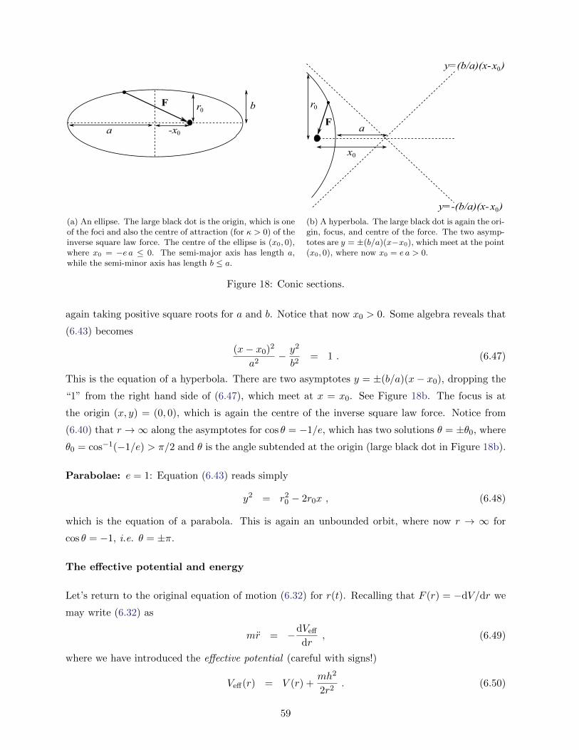
F
a -x0
br0
(a) An ellipse. The large black dot is the origin, which is oneof the foci and also the centre of attraction (for κ > 0) of theinverse square law force. The centre of the ellipse is (x0, 0),where x0 = −e a ≤ 0. The semi-major axis has length a,while the semi-minor axis has length b ≤ a.
Fa
x0y=(b/a)(x-
y=-(b/a)(x-
)
x0)
x0
r0
(b) A hyperbola. The large black dot is again the ori-gin, focus, and centre of the force. The two asymp-totes are y = ±(b/a)(x−x0), which meet at the point(x0, 0), where now x0 = e a > 0.
Figure 18: Conic sections.
again taking positive square roots for a and b. Notice that now x0 > 0. Some algebra reveals that
(6.43) becomes
(x− x0)2
a2− y2
b2= 1 . (6.47)
This is the equation of a hyperbola. There are two asymptotes y = ±(b/a)(x− x0), dropping the
“1” from the right hand side of (6.47), which meet at x = x0. See Figure 18b. The focus is at
the origin (x, y) = (0, 0), which is again the centre of the inverse square law force. Notice from
(6.40) that r →∞ along the asymptotes for cos θ = −1/e, which has two solutions θ = ±θ0, where
θ0 = cos−1(−1/e) > π/2 and θ is the angle subtended at the origin (large black dot in Figure 18b).
Parabolae: e = 1: Equation (6.43) reads simply
y2 = r20 − 2r0x , (6.48)
which is the equation of a parabola. This is again an unbounded orbit, where now r → ∞ for
cos θ = −1, i.e. θ = ±π.
The effective potential and energy
Let’s return to the original equation of motion (6.32) for r(t). Recalling that F (r) = −dV/dr we
may write (6.32) as
mr = −dVeff
dr, (6.49)
where we have introduced the effective potential (careful with signs!)
Veff(r) = V (r) +mh2
2r2. (6.50)
59
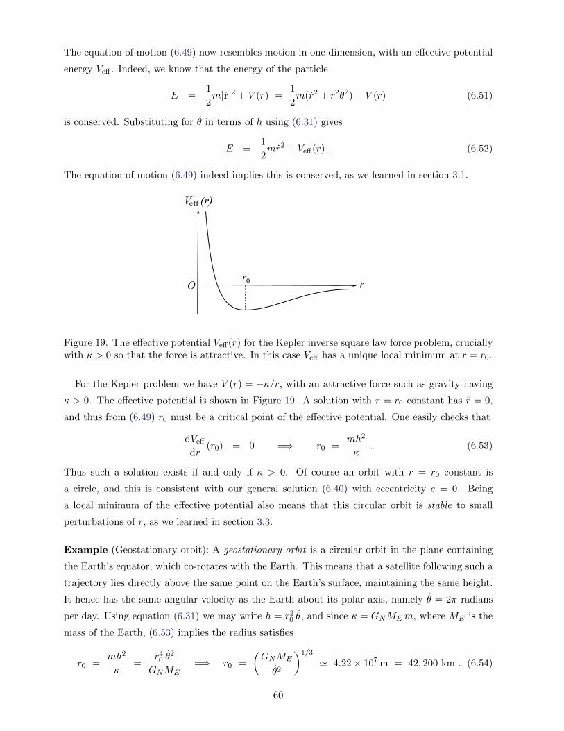
The equation of motion (6.49) now resembles motion in one dimension, with an effective potential
energy Veff . Indeed, we know that the energy of the particle
E =1
2m|r|2 + V (r) =
1
2m(r2 + r2θ2) + V (r) (6.51)
is conserved. Substituting for θ in terms of h using (6.31) gives
E =1
2mr2 + Veff(r) . (6.52)
The equation of motion (6.49) indeed implies this is conserved, as we learned in section 3.1.
O r
(r)Veff
r0
Figure 19: The effective potential Veff(r) for the Kepler inverse square law force problem, cruciallywith κ > 0 so that the force is attractive. In this case Veff has a unique local minimum at r = r0.
For the Kepler problem we have V (r) = −κ/r, with an attractive force such as gravity having
κ > 0. The effective potential is shown in Figure 19. A solution with r = r0 constant has r = 0,
and thus from (6.49) r0 must be a critical point of the effective potential. One easily checks that
dVeff
dr(r0) = 0 =⇒ r0 =
mh2
κ. (6.53)
Thus such a solution exists if and only if κ > 0. Of course an orbit with r = r0 constant is
a circle, and this is consistent with our general solution (6.40) with eccentricity e = 0. Being
a local minimum of the effective potential also means that this circular orbit is stable to small
perturbations of r, as we learned in section 3.3.
Example (Geostationary orbit): A geostationary orbit is a circular orbit in the plane containing
the Earth’s equator, which co-rotates with the Earth. This means that a satellite following such a
trajectory lies directly above the same point on the Earth’s surface, maintaining the same height.
It hence has the same angular velocity as the Earth about its polar axis, namely θ = 2π radians
per day. Using equation (6.31) we may write h = r20 θ, and since κ = GNMEm, where ME is the
mass of the Earth, (6.53) implies the radius satisfies
r0 =mh2
κ=
r40 θ
2
GNME=⇒ r0 =
(GNME
θ2
)1/3
' 4.22× 10⁷ m = 42, 200 km . (6.54)
60
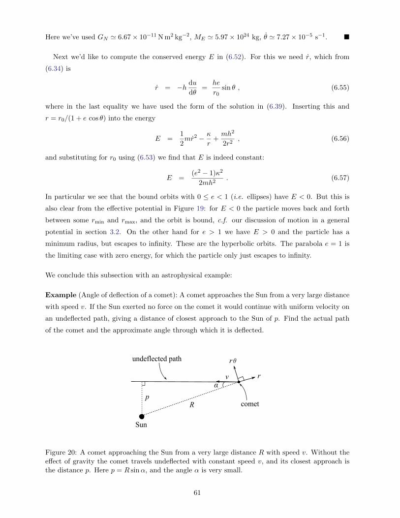
Here we’ve used GN ' 6.67× 10⁻¹¹ N m2 kg−2, ME ' 5.97× 1024 kg, θ ' 7.27× 10⁻⁵ s−1. �
Next we’d like to compute the conserved energy E in (6.52). For this we need r, which from
(6.34) is
r = −h du
dθ=
he
r0sin θ , (6.55)
where in the last equality we have used the form of the solution in (6.39). Inserting this and
r = r0/(1 + e cos θ) into the energy
E =1
2mr2 − κ
r+mh2
2r2, (6.56)
and substituting for r0 using (6.53) we find that E is indeed constant:
E =(e2 − 1)κ2
2mh2. (6.57)
In particular we see that the bound orbits with 0 ≤ e < 1 (i.e. ellipses) have E < 0. But this is
also clear from the effective potential in Figure 19: for E < 0 the particle moves back and forth
between some rmin and rmax, and the orbit is bound, c.f. our discussion of motion in a general
potential in section 3.2. On the other hand for e > 1 we have E > 0 and the particle has a
minimum radius, but escapes to infinity. These are the hyperbolic orbits. The parabola e = 1 is
the limiting case with zero energy, for which the particle only just escapes to infinity.
We conclude this subsection with an astrophysical example:
Example (Angle of deflection of a comet): A comet approaches the Sun from a very large distance
with speed v. If the Sun exerted no force on the comet it would continue with uniform velocity on
an undeflected path, giving a distance of closest approach to the Sun of p. Find the actual path
of the comet and the approximate angle through which it is deflected.
r
R
vα
rθ
Sun
pcomet
undeflected path
Figure 20: A comet approaching the Sun from a very large distance R with speed v. Without theeffect of gravity the comet travels undeflected with constant speed v, and its closest approach isthe distance p. Here p = R sinα, and the angle α is very small.
61
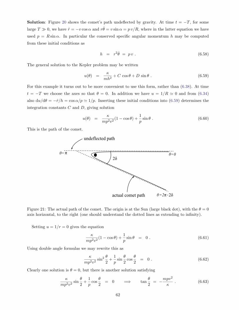
Solution: Figure 20 shows the comet’s path undeflected by gravity. At time t = −T , for some
large T � 0, we have r = −v cosα and rθ = v sinα = p v/R, where in the latter equation we have
used p = R sinα. In particular the conserved specific angular momentum h may be computed
from these initial conditions as
h = r2θ = p v . (6.58)
The general solution to the Kepler problem may be written
u(θ) =κ
mh2+ C cos θ +D sin θ . (6.59)
For this example it turns out to be more convenient to use this form, rather than (6.38). At time
t = −T we choose the axes so that θ = 0. In addition we have u = 1/R ' 0 and from (6.34)
also du/dθ = −r/h = cosα/p ' 1/p. Inserting these initial conditions into (6.59) determines the
integration constants C and D, giving solution
u(θ) =κ
mp2v2(1− cos θ) +
1
psin θ . (6.60)
This is the path of the comet.
θ
actual comet path
=0
θ =2π -2δ
θ=π2δ
undeflected path
Figure 21: The actual path of the comet. The origin is at the Sun (large black dot), with the θ = 0axis horizontal, to the right (one should understand the dotted lines as extending to infinity).
Setting u = 1/r = 0 gives the equation
κ
mp2v2(1− cos θ) +
1
psin θ = 0 . (6.61)
Using double angle formulas we may rewrite this as
κ
mp2v2sin2 θ
2+
1
psin
θ
2cos
θ
2= 0 . (6.62)
Clearly one solution is θ = 0, but there is another solution satisfying
κ
mp2v2sin
θ
2+
1
pcos
θ
2= 0 =⇒ tan
θ
2= −mpv
2
κ. (6.63)
62
Setting θ = 2π − 2δ this may be rewritten as
tan δ =mpv2
κ=
p v2
GNMS. (6.64)
Here in the second equality we have inserted the value κ = GNMSm, where MS is the mass of the
Sun.
The undeflected path in Figure 20 has the comet coming in at an angle θ = 0 (in the limit
R → ∞), and going past the Sun to θ = π. On the other hand, the actual path sends the comet
back out to infinity at an angle 2π − 2δ. It follows that the comet is deflected through an angle
π − 2δ. See Figure 21. �
6.3 Kepler’s laws
In the late 16th century the Danish nobleman Tycho Brahe made accurate and comprehensive
planetary observations, which Johannes Kepler was then able to analyse. Using this empirical
data Kepler remarkably deduced the following three laws (published between 1609 and 1619):
K1: The path of each planet is an ellipse with the Sun at the focus.
K2: A straight line joining the Sun and a planet sweeps out equal areas in equal times.
K3: The square of each planet’s period is proportional to the cube of the semi-major
axis of its elliptical orbit.
The force attracting a planet to the Sun is of course Newton’s inverse square law of gravitation,
which we solved in the previous subsection. Putting the Sun at the origin, this indeed turns out
to be the focus of an ellipse for bounded orbits. As we remarked earlier, just as the Sun attracts
the planet, by Newton’s third law the planet also attracts the Sun, which hence accelerates and
cannot be the origin of an inertial frame. This is true, but the Sun is so much more massive (more
than a factor of 103) than any planet that its centre can be taken to be approximately fixed. We’ll
discuss this more carefully in section 7.3. Notice that we are also ignoring the fact that in our
solar system there are many planets, which also attract each other – but this is again a subleading
effect.
We thus take it as read that we have proven K1 from Newton’s laws. What about K2 and K3?
Proof of K2: Kepler’s second law is a simple consequence of conservation of angular momentum,
expressed through equation (6.31). Recall the latter reads r2θ = h = constant. A straight line
from the Sun to a planet is simply the position vector r(t). In a small time interval δt the planet
sweeps out a small triangle with base length r and height rδθ (see Figure 22), which has area
δA = 12r · rδθ = 1
2r2θ δt. We thus deduce that
A =1
2r2θ =
1
2h = constant. (6.65)
63

r(t)
Sun
planet θδ
Aδarea
Figure 22: In a small time interval δt the angle subtended at the origin changes by a small amountδθ = θ δt, sweeping out an area δA.
Being a consequence only of conservation of angular momentum, Kepler’s second law holds for any
central force (even non-conservative ones). �
Proof of K3: The third law requires only a little more work. First we recall that the area of an
ellipse with semi-major axis a and semi-minor axis b is
A = πab . (6.66)
On the other hand, we know from K2 that this area is swept out at a constant rate A = 12h.
Integrating this over one period we obtain
A =
∫dA =
1
2h
∫dt =
1
2hT . (6.67)
Thus the square of the period T is
T 2 =4A2
h2=
4π2a2b2
h2=
4π2
GNMS· a
2b2
r0, (6.68)
where in the last step we have substituted h2 = κr0/m = GNMSr0 using (6.40). Using (6.44) we
may tidy up the last geometric factor in (6.68) as a2b2/r0 = r30/(1 − e2)3 = a3, giving the final
formula
T 2 =4π2a3
GNMS. (6.69)
This is precisely Kepler’s third law, where the proportionality factor is 4π2/GNMS , where MS =
mass of the Sun. �
6.4 Coulomb scattering
In the last two subsections we focused on the Kepler problem F (r) = −κ/r2 with κ > 0. For κ < 0
the inverse square law force is repulsive, rather than attractive. The equations are similar, but the
sign difference is important!
64
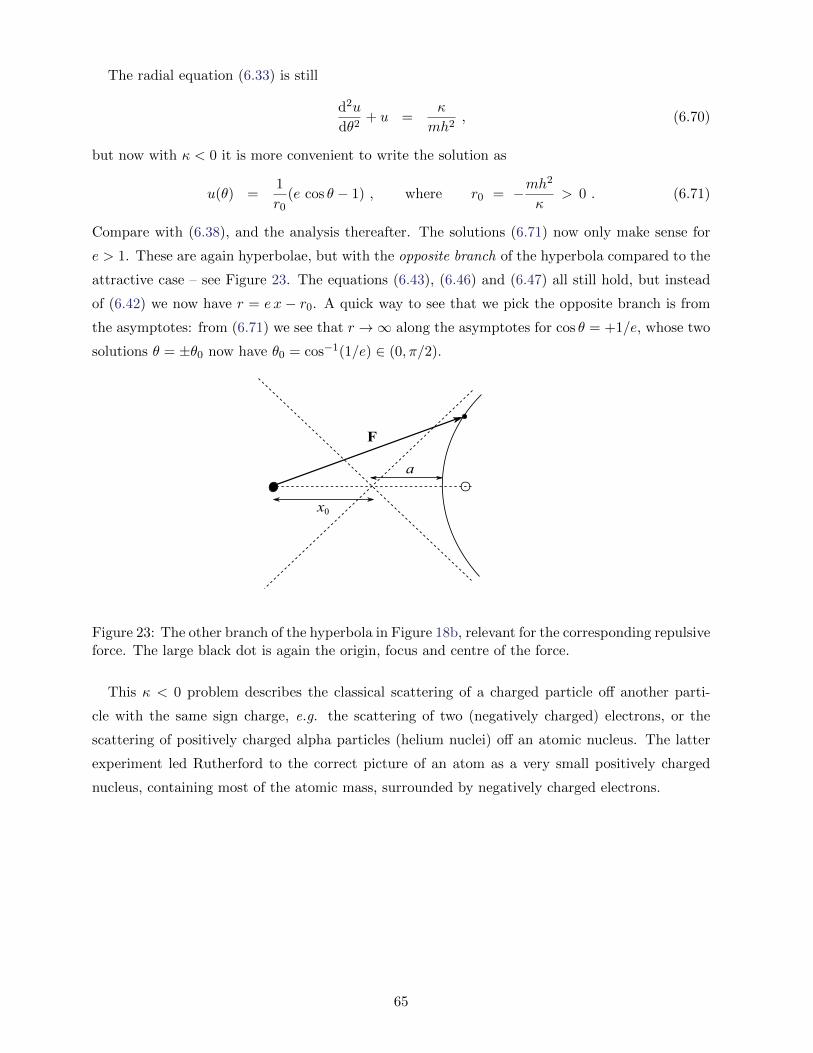
The radial equation (6.33) is still
d2u
dθ2+ u =
κ
mh2, (6.70)
but now with κ < 0 it is more convenient to write the solution as
u(θ) =1
r0(e cos θ − 1) , where r0 = −mh
2
κ> 0 . (6.71)
Compare with (6.38), and the analysis thereafter. The solutions (6.71) now only make sense for
e > 1. These are again hyperbolae, but with the opposite branch of the hyperbola compared to the
attractive case – see Figure 23. The equations (6.43), (6.46) and (6.47) all still hold, but instead
of (6.42) we now have r = e x − r0. A quick way to see that we pick the opposite branch is from
the asymptotes: from (6.71) we see that r →∞ along the asymptotes for cos θ = +1/e, whose two
solutions θ = ±θ0 now have θ0 = cos−1(1/e) ∈ (0, π/2).
a
x0
F
Figure 23: The other branch of the hyperbola in Figure 18b, relevant for the corresponding repulsiveforce. The large black dot is again the origin, focus and centre of the force.
This κ < 0 problem describes the classical scattering of a charged particle off another parti-
cle with the same sign charge, e.g. the scattering of two (negatively charged) electrons, or the
scattering of positively charged alpha particles (helium nuclei) off an atomic nucleus. The latter
experiment led Rutherford to the correct picture of an atom as a very small positively charged
nucleus, containing most of the atomic mass, surrounded by negatively charged electrons.
65
7 Systems of particles
So far we have mainly been studying the motion of a single particle. What can we say about
the dynamics of many particles? Before discussing this, now is a good time to discuss the non-
uniqueness of inertial frames.
7.1 Galilean transformations
As discussed in section 1, in order to apply Newton’s second law we must first establish an inertial
reference frame. Such frames are not unique. Suppose we have an inertial frame S, with respect
to which positions are specified by a vector r = (x, y, z) from the origin O. Consider the following
transformations to a different frame S ′, with positions specified by r′:spatial translations, r′ = r− x, where x is a constant vector,
constant rotations, r′ = R r, where R is a constant 3× 3 orthogonal matrix,
Galilean boosts, r′ = r− u t, where u is a constant velocity.
The first and second transformations simply translate the origin by a fixed distance, and rotate
the axes by a fixed rotation, respectively. The final transformation has the origins O, O′ moving
at a fixed relative velocity u.
If r(t) is the trajectory of a free particle (by definition, no forces act on it) in the frame S, then
d2
dt2r = 0. It is a simple matter to check that for each r′(t) above one has d2
dt2r′ = 0, and hence
the particle also moves with constant velocity in the new frame S ′. Any combination of the above
transformations thus maps an inertial frame to another inertial frame, generating the Galilean
transformation group.16 The freedom to make Galilean transformations is sometimes useful when
analysing the dynamics of more than one particle, as we shall see.
The insight of Galileo was that physics is invariant under Galilean transformations: the laws
of motion are the same in any inertial frame. This is known as Galileo’s principle of relativity.
For example, consider an observer standing on a train moving at constant velocity u, compared
to another observer at rest with respect to the Earth. These two inertial frames are in uniform
relative motion, so r′ = r− (u t+x), with u and x constant. The laws of motion (Newton’s second
law) inside the train are not any different from those for the observer at rest. However, as the train
turns through a bend in the track a reference frame at rest relative to the train is accelerating,
and this is observerd as a “fictitious force” by the passengers inside (luggage falls over, it’s less
easy to walk down the aisle, etc).
7.2 Centre of mass motion
Note on notation: Henceforth we will always denote our inertial frame, in which we write down
Newton’s second law, as S, with origin O.
16Sometimes time translations t′ = t− s, where s is a constant, are also included in this set of transformations.
66
Consider a system of N point particles. With respect to an inertial frame S, we denote the position
vector of the Ith particle from O by rI , which has mass mI and hence linear momentum pI = mI rI ,
I = 1, . . . , N . We suppose that particle J exerts a force FIJ on particle I, for I 6= J . Newton’s
third law immediately tells us that FJI = −FIJ for each I 6= J . On the other hand Newton’s
second law for particle I reads
mI rI = pI = FI = FextI +
∑J 6=I
FIJ . (7.1)
Here we have included an external force FextI , i.e. a force acting on particle I that is not due to
the other N − 1 particles in the system. We refer to the FIJ as internal forces.
When considering a single particle, the force F = Fext in Newton’s second law is by definition
always external. In this case we always have in mind that (a) something else is responsible for
producing that force, and (b) we are entirely ignoring the effect the particle has on whatever that
something else is (i.e. we are ignoring its back-reaction, under Newton’s third law). Of course,
whether or not it is reasonable to neglect the effects of the particle on the “external system” that
produces Fext depends on the circumstances. At the end of section 3.1 we briefly discussed fluid
drag in this context. At a molecular level the fluid is made up of fluid particles, and the drag force
is an effective external force, resulting from large numbers of collisions of our object with the very
small mass fluid particles. It is hardly reasonable to model this by introducing N ∼ 1030 water
molecules! A more subtle example is the Kepler problem in section 6.2. Here a particle of mass
m is attracted by an inverse square law force F = −(κ/r2) er directed towards the origin. In this
context we were effectively regarding F as an external force acting on the particle, ignoring the
fact that the mass at the origin that produces F will experience an equal and opposite force, and
hence accelerate. We’ll come back to precisely this point in the next subsection.
Definition The centre of mass of the system of particles is the point G, with position vector
RG ≡ 1
M
N∑I=1
mIrI , (7.2)
where M =∑N
I=1mI is the total mass. Similarly the total momentum of the system is
P ≡N∑I=1
pI = MRG . (7.3)
The key point of this is the following:
Theorem The centre of mass of the system behaves like a point particle of mass M acted on by
the total external force. In particular, the dynamics of the centre of mass is independent of the
internal forces.
67

Proof: We compute
MRG = P =
N∑I=1
pI =
N∑I=1
(FextI +
∑J 6=I
FIJ
), (7.4)
the last equality using (7.1). However, due to Newton’s third law FIJ = −FJI , the N(N − 1)
terms in the sum
N∑I=1
∑J 6=I
FIJ = 0 (7.5)
cancel pairwise. Thus (7.4) becomes
MRG = P =N∑I=1
FextI = Fext , (7.6)
where Fext is by definition the total external force. �
This result explains why we can (often) so accurately model objects as point particles, even when
they manifestly are not. Whatever internal forces are acting within our object, for example holding
it together, they will cancel out of the centre of mass motion. In most of the problems we have
studied we have then really been modelling the centre of mass motion of an object, and we’ve been
applying Newton’s second law in the form (7.6).
Definition A closed system is one in which all forces are internal, acting between the constituents
of the system. That is, FextI = 0, I = 1, . . . , N .
We then have the following important corollary:
Corollary For a closed system the total momentum is conserved, P = 0.
This is of course an immediate consequence of (7.6). When the total momentum is conserved
notice that the centre of mass moves with constant velocity RG = constant. This means that by
a suitable Galilean transformation (a Galilean boost and translation) we may take the centre of
mass to be RG = 0, the origin of our inertial frame.
Definition For a system with Fext = 0, the inertial frame in which the centre of mass RG = 0 is
called the centre of mass frame. (This is unique up to an overall constant rotation of the axes.)
Definition The total angular momentum L = LP of the system about a point P is
LP =
N∑I=1
(rI − x) ∧ pI , (7.7)
where P has position vector x from the origin O. That is, L is the vector sum of the angular
momenta LI = (rI − x) ∧ pI for each particle I about P – see (4.17).
68
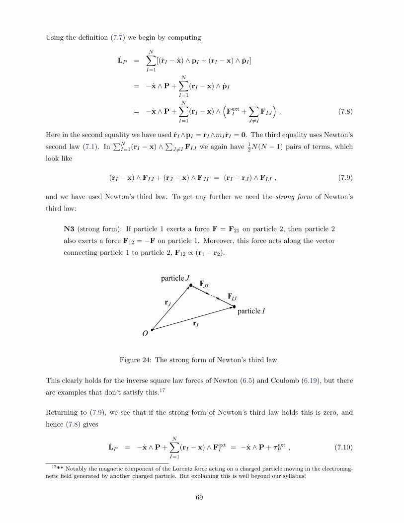
Using the definition (7.7) we begin by computing
LP =
N∑I=1
[(rI − x) ∧ pI + (rI − x) ∧ pI ]
= −x ∧P +
N∑I=1
(rI − x) ∧ pI
= −x ∧P +
N∑I=1
(rI − x) ∧(FextI +
∑J 6=I
FIJ
). (7.8)
Here in the second equality we have used rI∧pI = rI∧mI rI = 0. The third equality uses Newton’s
second law (7.1). In∑N
I=1(rI − x) ∧∑
J 6=I FIJ we again have 12N(N − 1) pairs of terms, which
look like
(rI − x) ∧ FIJ + (rJ − x) ∧ FJI = (rI − rJ) ∧ FIJ , (7.9)
and we have used Newton’s third law. To get any further we need the strong form of Newton’s
third law:
N3 (strong form): If particle 1 exerts a force F = F21 on particle 2, then particle 2
also exerts a force F12 = −F on particle 1. Moreover, this force acts along the vector
connecting particle 1 to particle 2, F12 ∝ (r1 − r2).
rO
I
rJFIJ
FJI
particle I
particle J
Figure 24: The strong form of Newton’s third law.
This clearly holds for the inverse square law forces of Newton (6.5) and Coulomb (6.19), but there
are examples that don’t satisfy this.17
Returning to (7.9), we see that if the strong form of Newton’s third law holds this is zero, and
hence (7.8) gives
LP = −x ∧P +N∑I=1
(rI − x) ∧ FextI = −x ∧P + τ ext
P , (7.10)
17** Notably the magnetic component of the Lorentz force acting on a charged particle moving in the electromag-netic field generated by another charged particle. But explaining this is well beyond our syllabus!
69
where τ extP is by definition the total external torque about P , c.f. (4.22).
There are two special cases where the first term on the right hand side of (7.10) is zero: (i) taking
P = O gives x = 0, (ii) taking instead P = G we have x ∧ P = RG ∧ P = RG ∧MRG = 0. We
have thus proven:
Theorem Provided the strong form of Newton’s third law holds, the rate of change of total
angular momentum about either O/G equals the total external torque about O/G. That is,
LO/G = τ extO/G
. (7.11)
Corollary For a closed system satisfying the strong form of Newton’s third law, the total angular
momentum about the origin O of an inertial frame is conserved, LO = 0.
The main application of (7.11) will be to rigid body motion, which is the subject of section 8.3.
In particular the following result will be useful:
Proposition Consider the system of particles in a uniform gravitational field, with acceleration
due to gravity g. Assuming this is the only external force acting, the total external torque about
a point P with position vector x is
τ extP = −(RG − x) ∧Mg k . (7.12)
This is the same as the torque for a particle of mass M at the centre of mass RG (compare to
(4.22)). In particular, the torque about G (for which x = RG) is zero.
Proof: We simply compute
τ extP ≡
N∑I=1
(rI − x) ∧ FextI =
N∑I=1
(rI − x) ∧ (−mIg k) = −(RG − x) ∧Mg k , (7.13)
where we have used the definitions M =∑N
I=1mI , MRG =∑N
I=1mIrI in the final equality. �
7.3 The two-body problem
A closed system with a single point particle isn’t very interesting: there is no force acting, and the
particle moves with constant momentum. The two-body problem is a closed system of two point
particles. Newton’s second and third laws give
m1r1 = F12 , m2r2 = F21 = −F12 . (7.14)
Adding these two equations implies that the centre of mass
RG =m1r1 +m2r2
m1 +m2(7.15)
70
moves with constant velocity, which we knew from the last subsection. On the other hand, if we
define r ≡ r1 − r2 so that
r1 = RG +m2
m1 +m2r , r2 = RG −
m1
m1 +m2r , (7.16)
then from (7.14) we deduce
r = r1 − r2 =
(1
m1+
1
m2
)F12 =
m1 +m2
m1m2F12 . (7.17)
Definition The reduced mass for the two-body problem is µ =m1m2
m1 +m2.
In terms of this the equation of motion (7.17) reads
µr = F12 . (7.18)
Example: For the inverse square law force F12 = − κ
|r1 − r2|3(r1 − r2) = − κ
r2
r
r, where r = |r|.
We have thus effectively reduced the two-body problem to a problem for a single particle, with
position vector r(t) satisfying (7.18). The force on the right hand side is then effectively an external
force for this particle. Having solved this, the solution to the original two-body problem is given
by (7.16). In fact we are always free to define r∗1 = r1−RG, r∗2 = r2−RG, which are the positions
of the two particles in the centre of mass frame. Recall this is a Galilean transformation, since
RG = constant. In this inertial frame (7.16) becomes
r∗1 =m2
m1 +m2r , r∗2 = − m1
m1 +m2r . (7.19)
If the second mass is much larger than the first, m2 � m1, then these become r∗1 ' r, r∗2 ' 0,
while the reduced mass is µ ' m1. We may thus view what we did in solving the Kepler problem
in section 6.2 in two different ways:
• If we take the mass m = µ in (6.27), then in section 6.2 we were really solving (7.18) for the
two-body problem. This describes the exact internal relative motion of the two bodies.
• If we instead take the mass m2 � m1 then the solution in section 6.2 is the approximate
solution to the two-body problem in the centre of mass frame, where the larger mass m2 is
at the origin.
Usually the latter is applicable, e.g. the Sun is more than 1000 times more massive than any
of the planets, while for a satellite or comet orbiting the Earth the factor is many orders of
magnitude larger still. What’s remarkable about the two-body problem is that the exact solution
and approximate solution we have described are mathematically equivalent, differing only in which
mass to use in Newton’s second law!
71

8 Rotating frames and rigid bodies
In this final section we discuss two topics that involve rotation: the dynamics of rigid bodies in
sections 8.2 and 8.3, and Newton’s laws in a general (i.e. non-inertial) frame from section 8.4 to the
end. We will only describe the basic features of rigid body motion, focusing on simple examples;
a general discussion is left to B7.1 Classical Mechanics (which also introduces and exploits more
powerful methods for solving the dynamics).
8.1 Rotating frames
Throughout this section there will always be two reference frames in the problem, and it is impor-
tant to make clear which is which from the outset:
A fixed inertial frame S: this has origin O and fixed coordinate axes with corresponding
basis vectors ei, i = 1, 2, 3.
A general frame S: this has origin O, with position vector x as measured from O, and
coordinate axes with corresponding basis vectors ei, i = 1, 2, 3.
Whenever we write down Newton’s laws of motion, we must do so using the inertial frame S. This
is the frame of an inertial observer, often called the laboratory frame by physicists, and we regard
it as fixed and time-independent. In particular this means that the basis vectors ei are independent
of time, ddt ei = 0, i = 1, 2, 3. When we introduce rigid bodies, the frame S will rotate with the
body, and hence will in general be non-inertial.
frame S
e
x
O
O
frame S
1
e2
e3
e1
e2
e3
(t)
Figure 25: The reference frame S is a fixed inertial frame. This is the frame in which we formulateNewton’s laws of motion, and hence do the “observing”. With respect to this frame, a generalframe S has origin O at position vector x = x(t) as measured from O, and its coordinate axes maybe rotating, so that ei = ei(t).
72

We may write the orthonormal basis vectors {ei} of the frame S as
ei(t) =
3∑j=1
Rij(t) ej , i = 1, 2, 3 . (8.1)
As you learned in the Geometry course, the fact that both bases are orthonormal means that
R = (Rij) is an orthogonal matrix. The main result of this subsection is:
Proposition There is a (unique) vector ω = ω(t) such that
ei = ω ∧ ei , i = 1, 2, 3 . (8.2)
ω = ω(t) is called the angular velocity of the frame S with respect to fixed inertial frame S.
We give two proofs below. The first doesn’t use orthogonal matrices directly, while the second
does. (The second proof appeared in the Geometry course.)
Proof 1: The fact that {ei} is an orthonormal basis means that
ei · ej = δij =
{1 if i = j
0 otherwise. (8.3)
Differentiating this with respect to time t thus gives
ei · ej + ei · ej = 0 . (8.4)
In particular taking i = j gives the three equations e1 · e1 = e2 · e2 = e3 · e3 = 0. This means that
ei is orthogonal to ei for each i = 1, 2, 3, and hence we may write
e1 = γ e2 − β e3 , e2 = α e3 − λ e1 , e3 = ν e1 − µ e2 , (8.5)
where α, β, γ, λ, µ and ν are functions of time t. The remaining content of (8.4) gives
e1 · e2 + e1 · e2 = 0 =⇒ λ = γ ,
e2 · e3 + e2 · e3 = 0 =⇒ µ = α ,
e3 · e1 + e3 · e1 = 0 =⇒ ν = β . (8.6)
It follows that
e1 = γ e2 − β e3 , e2 = α e3 − γ e1 , e3 = β e1 − α e2 , (8.7)
which may be written more succinctly as (8.2), where ω = (α, β, γ) = α e1 + β e2 + γ e3, and we
have used e1 ∧ e2 = e3, plus the cyclic permutations e2 ∧ e3 = e1, e3 ∧ e1 = e2. �
Proof 2: The alternative proof of this Proposition instead takes the time derivative of (8.1):
ei =3∑j=1
Rij ej =
3∑j,k=1
RijRkj ek =
3∑k=1
(RRT)ik ek , (8.8)
73
where in the second equality we have used the fact that R is orthogonal, and hence R−1 = RT. In
the Geometry course the angular velocity vector ω was instead introduced by noting that (RRT)
is an anti-symmetric matrix, so that we can write
RRT =
0 γ −β−γ 0 α
β −α 0
. (8.9)
Then (8.8) is equivalent to (8.2) with ω = (α, β, γ) – to see this just look at (8.7): the three rows
of (8.9) give the right hand sides of the three equations in (8.7), respectively. �
Example: Consider the special case in which
R(t) =
cos θ(t) sin θ(t) 0
− sin θ(t) cos θ(t) 0
0 0 1
, (8.10)
so that e1 = cos θ(t) e1 + sin θ(t) e2, e2 = − sin θ(t) e1 + cos θ(t) e2, e3 = e3. This is a rotation
about the third axis e3 = e3 by an angle θ = θ(t). Then we compute e1 = θ e2, e2 = −θ e1, e3 = 0,
and hence from (8.2) that ω = θ e3. �
We can gain some more intuition for the formula (8.2) by thinking about the position vector
r of a particle. Suppose for simplicity that the two origins coincide (for all time), so that O =
O. We have two bases, {ei} and {ei}, and we may expand the same vector r in both bases as
r =∑3
i=1 ri ei =∑3
i=1 ri ei. Here ri are the components of r in the frame S, while ri are the
components in the frame S. In section 1.1 we would have referred to the position vector in the
two frames as r and r, respectively, because we wanted to emphasize that it is the components ri
and ri that we measure in the frames. However, r and r are the same vector, just expressed in
different bases. The velocity of the particle in the inertial frame S is
r =
3∑i=1
ri ei +
3∑i=1
ri ei =
3∑i=1
ri ei +
3∑i=1
riω ∧ ei
=
(dr
dt
)S
+ ω ∧ r . (8.11)
Here we have introduced:
Definition The time derivative of r = r(t) in the frame S is
(dr
dt
)S≡ r1 e1 + r2 e2 + r3 e3. That
is, we simply differentiate the components of r in the orthonormal basis {ei} for S.
We should then never simply write “r” when there are two general reference frames being used,
because whether or not something is moving depends on who is doing the measuring. However,
when we do write “r” we will always mean the time derivative in the inertial frame S. Then (8.11)
more properly reads
74
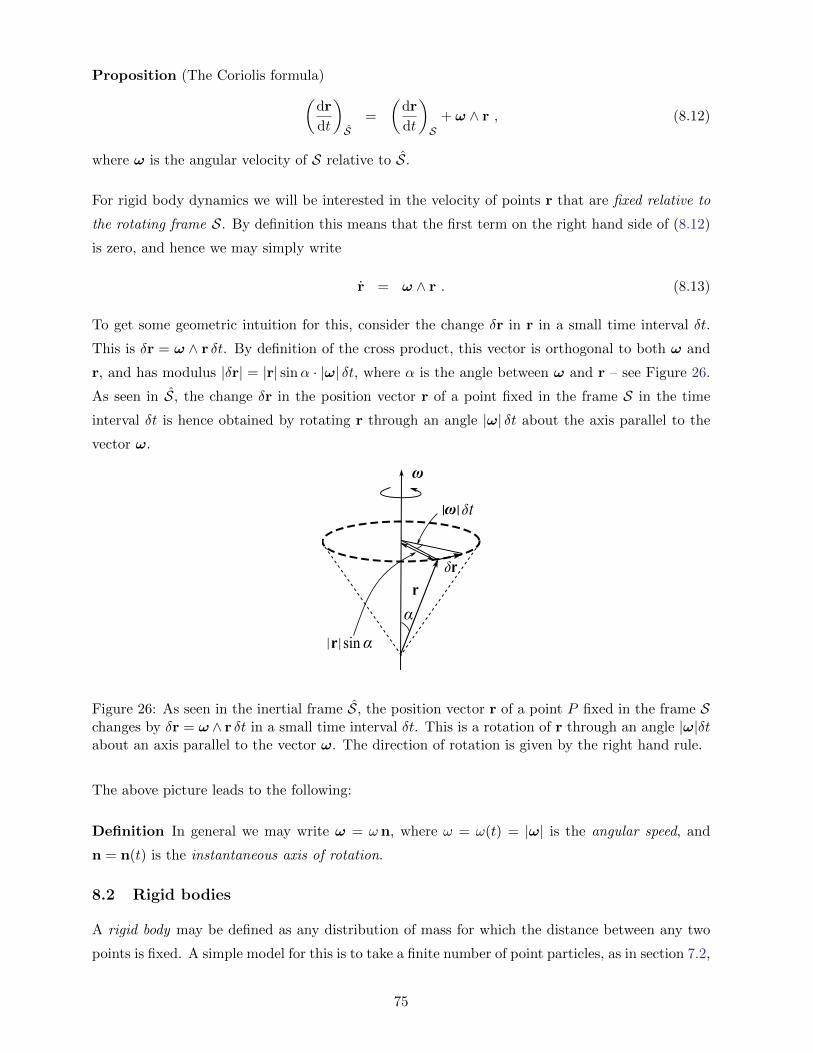
Proposition (The Coriolis formula)(dr
dt
)S
=
(dr
dt
)S
+ ω ∧ r , (8.12)
where ω is the angular velocity of S relative to S.
For rigid body dynamics we will be interested in the velocity of points r that are fixed relative to
the rotating frame S. By definition this means that the first term on the right hand side of (8.12)
is zero, and hence we may simply write
r = ω ∧ r . (8.13)
To get some geometric intuition for this, consider the change δr in r in a small time interval δt.
This is δr = ω ∧ r δt. By definition of the cross product, this vector is orthogonal to both ω and
r, and has modulus |δr| = |r| sinα · |ω| δt, where α is the angle between ω and r – see Figure 26.
As seen in S, the change δr in the position vector r of a point fixed in the frame S in the time
interval δt is hence obtained by rotating r through an angle |ω| δt about the axis parallel to the
vector ω.
ω
r
δ
δt| |
ω
r
sinr|
α
α|
Figure 26: As seen in the inertial frame S, the position vector r of a point P fixed in the frame Schanges by δr = ω ∧ r δt in a small time interval δt. This is a rotation of r through an angle |ω|δtabout an axis parallel to the vector ω. The direction of rotation is given by the right hand rule.
The above picture leads to the following:
Definition In general we may write ω = ω n, where ω = ω(t) = |ω| is the angular speed, and
n = n(t) is the instantaneous axis of rotation.
8.2 Rigid bodies
A rigid body may be defined as any distribution of mass for which the distance between any two
points is fixed. A simple model for this is to take a finite number of point particles, as in section 7.2,
75

but with the constraint that the position vectors rI (I = 1, . . . , N) satisfy |rI−rJ | = cIJ = constant.
This ensures that the body retains its size, shape and distribution of mass. One might imagine the
rI as the positions of atoms in a solid, with the constraints arising from inter-molecular forces. We
assume these constraint forces satisfy the strong form of Newton’s third law. For now we will stick
with this point particle model, but later we will model a rigid body as a continuous distribution
of matter, which may be regarded as a limit of the point particle model in which the number of
particles tends to infinity.
Choose a point O that is fixed in the body. For example, in the point particle model this could
be one of the particles, although as we shall see below it will often be convenient to take this to be
the centre of mass. We denote the position vector of O as x = x(t), where this is measured from
the origin O of the inertial frame S. We may then write
RI = x + rI , I = 1, . . . , N , (8.14)
so that RI and rI are the positions of the body particles, as measured from O and O, respectively.
See Figure 27.
ω
R
O
P
O
x
I
ω
O
P
O
I
rI
x
(i) (ii)
I
rI
R I
Figure 27: We fix a point O in the rigid body, which is taken to be the origin of the rest frame Sof the body. The frame S has angular velocity ω, and its origin O has position vector x relativeto the origin O of an inertial frame S. The body particles PI have position vectors rI , measuredfrom O. Figures (i) and (ii) show the same body at two different times.
Definition The rest frame S of the rigid body is a reference frame, with origin O, with respect
to which the rI are fixed (at rest), i.e.
(drIdt
)S
= 0 for all I = 1, . . . , N .
The existence of such a frame is really equivalent to what we mean by a rigid body in the first
place. Provided the matter distribution is not all along a line, the rest frame is defined uniquely
by the body, up to a constant rotation of its axes and a translation of the origin by a constant
vector (relative to S).
76
Using the Coriolis formula (8.12) we then have the important result that
RI = x + rI = vO + ω ∧ rI . (8.15)
Here vO = x is the velocity of O, as measured in the inertial frame S, while ω is the angular
velocity of the rest frame S with respect to S.
As we already mentioned, a natural choice for O is the centre of mass G of the body. This means
that x = RG, in the notation of section 7.2.18 From (7.2) and (8.14) we have
RG =1
M
N∑I=1
mIRI =1
M
N∑I=1
mI(RG + rI) = RG +1
M
N∑I=1
mIrI , (8.16)
which implies the constraint
N∑I=1
mIrI = 0 (8.17)
on the rI . Let’s re-examine the formulas for the total momentum (linear and angular) from
section 7.2, and also look at the total kinetic energy. We take O = G, unless otherwise stated.
Linear momentum
We already know from (7.3) that P = MRG = MvG, but it’s interesting to see this explicitly in
our current set up:
P =N∑I=1
mIRI =N∑I=1
mI(RG + ω ∧ rI) = MRG + ω ∧
(N∑I=1
mIrI
)= MRG . (8.18)
Here we’ve used equation (8.15) with x = RG in the second equality, while the last equality uses
the constraint (8.17). The total momentum is hence as if the whole mass M were concentrated at
the centre of mass G.
Angular momentum
The total angular momentum about the centre of mass O = G is by definition
LG =N∑I=1
rI ∧mIRI =N∑I=1
mIrI ∧ (RG + ω ∧ rI) =N∑I=1
mIrI ∧ (ω ∧ rI) . (8.19)
We emphasize again that we have chosen to compute the angular momentum about O = G, not
about the origin O of the inertial frame. That latter would be LO, and have RI in place of rI
after the first equals sign. The last equality follows from the constraint (8.17). Using the vector
identity rI ∧ (ω ∧ rI) = (rI · rI)ω − (rI · ω)rI , we may hence write
LG =
N∑I=1
mI [(rI · rI)ω − (rI · ω)rI ] . (8.20)
18Notice that in this section we are denoting the positions of the particles measured from the origin O of theinertial frame by RI . Thus one should replace rI by RI in the formulas in section 7.2.
77
Definition The inertia tensor I = I(O) = (I(O)ij ) of the rigid body, about a point O fixed in the
body, is defined as
Iij =N∑I=1
mI [(rI · rI)δij − rI i rI j ] . (8.21)
Here rI =∑3
i=1 rI i ei are the position vectors of the body particles, in the rest frame basis {ei}.
Notice the inertia tensor is defined in the rest frame of the body, and so is intrinsic to the body
itself, and in particular independent of time t. It is also manifestly symmetric, I = IT. Note also
that the definition depends on a choice of origin O, fixed in the body. The point of the definition
is that we may now write the total angular momentum (8.20) in matrix notation as
LG = I(G)ω =
3∑i,j=1
I(G)ij ωj ei . (8.22)
Kinetic energy
The total kinetic energy of the body, as measured in the inertial frame, is
T =N∑I=1
1
2mI |RI |2 =
1
2
N∑I=1
mI
[|RG|2 + 2RG · (ω ∧ rI) + (ω ∧ rI) · (ω ∧ rI)
]. (8.23)
The middle term on the right hand side is again zero, using the constraint (8.17). On the other
hand we may rewrite the last term using the vector identify
(ω ∧ rI) · (ω ∧ rI) = ω · (rI ∧ (ω ∧ rI)) . (8.24)
Recalling the formula (8.20), we have thus shown that
T =1
2M |RG|2 +
1
2ω · LG . (8.25)
That is, the total kinetic energy is the sum of two terms: the first is due to the centre of mass
motion relative to O, and is again is as though all the mass was concentrated at the centre of mass.
The second term is the rotational kinetic energy about G.
Definition The rotational kinetic energy about the centre of mass G is
Trot =1
2ω · LG =
1
2ωTI(G)ω =
1
2
3∑i,j=1
I(G)ij ωi ωj . (8.26)
These general formulae are very pretty, but they are also quite abstract. We conclude this subsec-
tion with some simple examples. Here we usually have in mind a continuous distribution of matter,
rather than a point particle model. This assumes the distribution of mass in the body is defined by
a density ρ(r), so that the mass δm in a small volume dx dy dz centred at r = (r1, r2, r3) = (x, y, z)
78
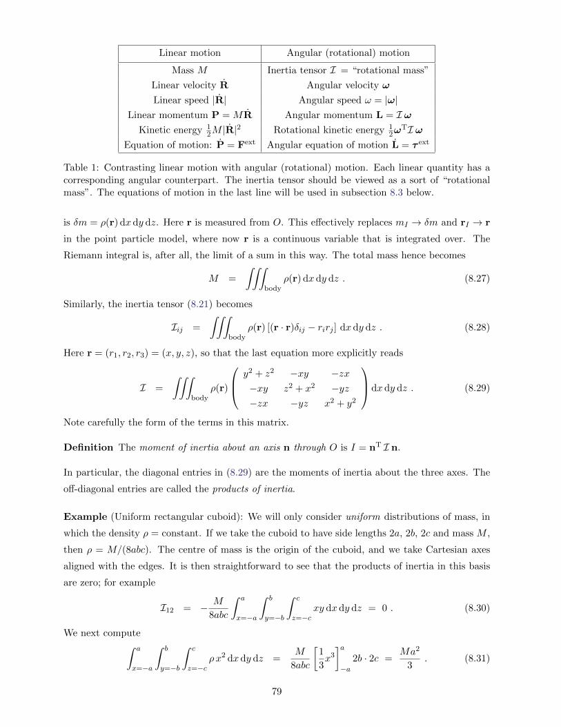
Linear motion Angular (rotational) motion
Mass M Inertia tensor I = “rotational mass”
Linear velocity R Angular velocity ω
Linear speed |R| Angular speed ω = |ω|Linear momentum P = MR Angular momentum L = I ω
Kinetic energy 12M |R|
2 Rotational kinetic energy 12ω
TI ωEquation of motion: P = Fext Angular equation of motion L = τ ext
Table 1: Contrasting linear motion with angular (rotational) motion. Each linear quantity has acorresponding angular counterpart. The inertia tensor should be viewed as a sort of “rotationalmass”. The equations of motion in the last line will be used in subsection 8.3 below.
is δm = ρ(r) dx dy dz. Here r is measured from O. This effectively replaces mI → δm and rI → r
in the point particle model, where now r is a continuous variable that is integrated over. The
Riemann integral is, after all, the limit of a sum in this way. The total mass hence becomes
M =
∫∫∫body
ρ(r) dx dy dz . (8.27)
Similarly, the inertia tensor (8.21) becomes
Iij =
∫∫∫body
ρ(r) [(r · r)δij − rirj ] dx dy dz . (8.28)
Here r = (r1, r2, r3) = (x, y, z), so that the last equation more explicitly reads
I =
∫∫∫body
ρ(r)
y2 + z2 −xy −zx−xy z2 + x2 −yz−zx −yz x2 + y2
dx dy dz . (8.29)
Note carefully the form of the terms in this matrix.
Definition The moment of inertia about an axis n through O is I = nT I n.
In particular, the diagonal entries in (8.29) are the moments of inertia about the three axes. The
off-diagonal entries are called the products of inertia.
Example (Uniform rectangular cuboid): We will only consider uniform distributions of mass, in
which the density ρ = constant. If we take the cuboid to have side lengths 2a, 2b, 2c and mass M ,
then ρ = M/(8abc). The centre of mass is the origin of the cuboid, and we take Cartesian axes
aligned with the edges. It is then straightforward to see that the products of inertia in this basis
are zero; for example
I12 = − M
8abc
∫ a
x=−a
∫ b
y=−b
∫ c
z=−cxy dx dy dz = 0 . (8.30)
We next compute∫ a
x=−a
∫ b
y=−b
∫ c
z=−cρ x2 dx dy dz =
M
8abc
[1
3x3
]a−a
2b · 2c =Ma2
3. (8.31)
79
The integrals involving y2 and z2 are of course similar, and we deduce that
I(G) =
13M(b2 + c2) 0 0
0 13M(c2 + a2) 0
0 0 13M(a2 + b2)
. (8.32)
�
The inertia tensor (8.32) is diagonal in this last example. Since I is always a real symmetric matrix,
by the Spectral Theorem in Linear Algebra II there is always a change of basis by a (constant)
orthogonal matrix P such that P I PT is diagonal.
Definition In this latter basis I =
I1 0 0
0 I2 0
0 0 I3
, and the eigenvalues Ii of I, i = 1, 2, 3, are
called the principal moments of inertia. The corresponding eigenvectors, with which the axes ei
are aligned, are called the principal axes.
A rigid body thus in general determines its own natural choice of rest frame: the origin is the
centre of mass G, while the axes are the principal axes. In this frame the inertia tensor about G is
diagonal. This is the natural choice of rest frame, but it isn’t always the most convenient choice.
We may also consider two-dimensional bodies, such as a thin flat disc, or one-dimensional bodies
such as a rigid rod. In this case one replaces the density ρ by a surface density, or line density,
respectively, and integrates over the surface or curve, respectively.
Example (Thin uniform disc): As a two-dimensional example, consider a thin uniform disc of
radius a and mass M . Thus the surface density is ρ = M/(πa2), and due to the rotational
symmetry the centre of mass must be at the origin of the disc. Taking this to be the origin,
with the disc lying in the (x, y) plane at z = 0, we may introduce polar coordinates x = r cos θ,
y = r sin θ in this plane. We then compute
I11 =
∫∫ρ y2 dx dy =
M
πa2
∫ a
r=0
∫ 2π
θ=0r2 sin2 θ r dr dθ =
1
4Ma2 . (8.33)
Notice here that the integrand is ρ(y2 + z2) = ρ y2, as the body is two-dimensional and lies in the
plane z = 0. By symmetry we must have I11 = I22 (which is easy enough to check explicitly), and
we also compute
I33 =
∫∫ρ (x2 + y2) dx dy =
M
πa2· 2π
∫ a
r=0r2 r dr =
1
2Ma2 . (8.34)
Two of the products of inertia (I13 and I23) are obviously zero, because the disc lies in the plane
z = 0. The less obvious one is
I12 = −∫∫
ρ xy dx dy = − M
πa2
∫ a
r=0
∫ 2π
θ=0r3 sin θ cos θ dr dθ = 0 . (8.35)
80
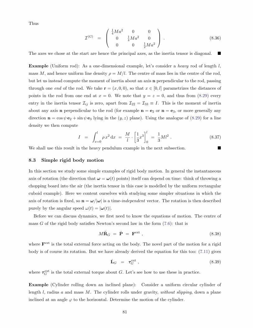
Thus
I(G) =
14Ma2 0 0
0 14Ma2 0
0 0 12Ma2
. (8.36)
The axes we chose at the start are hence the principal axes, as the inertia tensor is diagonal. �
Example (Uniform rod): As a one-dimensional example, let’s consider a heavy rod of length l,
mass M , and hence uniform line density ρ = M/l. The centre of mass lies in the centre of the rod,
but let us instead compute the moment of inertia about an axis n perpendicular to the rod, passing
through one end of the rod. We take r = (x, 0, 0), so that x ∈ [0, l] parametrizes the distances of
points in the rod from one end at x = 0. We note that y = z = 0, and thus from (8.29) every
entry in the inertia tensor Iij is zero, apart from I22 = I33 ≡ I. This is the moment of inertia
about any axis n perpendicular to the rod (for example n = e2 or n = e3, or more generally any
direction n = cosψ e2 + sinψ e3 lying in the (y, z) plane). Using the analogue of (8.29) for a line
density we then compute
I =
∫ l
x=0ρ x2 dx =
M
l·[
1
3x3
]l0
=1
3Ml2 . (8.37)
We shall use this result in the heavy pendulum example in the next subsection. �
8.3 Simple rigid body motion
In this section we study some simple examples of rigid body motion. In general the instantaneous
axis of rotation (the direction that ω = ω(t) points) itself can depend on time: think of throwing a
chopping board into the air (the inertia tensor in this case is modelled by the uniform rectangular
cuboid example). Here we content ourselves with studying some simpler situations in which the
axis of rotation is fixed, so n = ω/|ω| is a time-independent vector. The rotation is then described
purely by the angular speed ω(t) = |ω(t)|.
Before we can discuss dynamics, we first need to know the equations of motion. The centre of
mass G of the rigid body satisfies Newton’s second law in the form (7.6): that is
MRG = P = Fext , (8.38)
where Fext is the total external force acting on the body. The novel part of the motion for a rigid
body is of course its rotation. But we have already derived the equation for this too: (7.11) gives
LG = τ extG , (8.39)
where τ extG is the total external torque about G. Let’s see how to use these in practice.
Example (Cylinder rolling down an inclined plane): Consider a uniform circular cylinder of
length l, radius a and mass M . The cylinder rolls under gravity, without slipping, down a plane
inclined at an angle ϕ to the horizontal. Determine the motion of the cylinder.
81
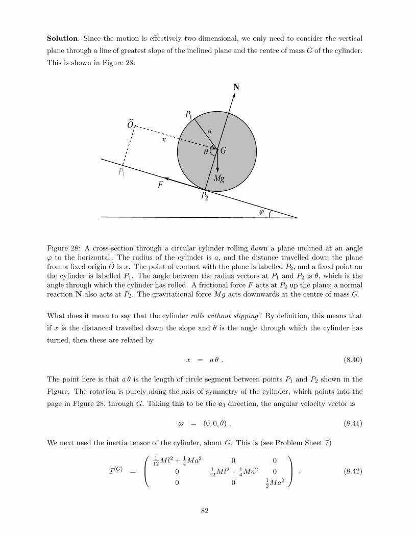
Solution: Since the motion is effectively two-dimensional, we only need to consider the vertical
plane through a line of greatest slope of the inclined plane and the centre of mass G of the cylinder.
This is shown in Figure 28.
N
Mg
G
O
x
P1
P2F
P1
θ
a
φ
Figure 28: A cross-section through a circular cylinder rolling down a plane inclined at an angleϕ to the horizontal. The radius of the cylinder is a, and the distance travelled down the planefrom a fixed origin O is x. The point of contact with the plane is labelled P2, and a fixed point onthe cylinder is labelled P1. The angle between the radius vectors at P1 and P2 is θ, which is theangle through which the cylinder has rolled. A frictional force F acts at P2 up the plane; a normalreaction N also acts at P2. The gravitational force Mg acts downwards at the centre of mass G.
What does it mean to say that the cylinder rolls without slipping? By definition, this means that
if x is the distanced travelled down the slope and θ is the angle through which the cylinder has
turned, then these are related by
x = a θ . (8.40)
The point here is that a θ is the length of circle segment between points P1 and P2 shown in the
Figure. The rotation is purely along the axis of symmetry of the cylinder, which points into the
page in Figure 28, through G. Taking this to be the e3 direction, the angular velocity vector is
ω = (0, 0, θ) . (8.41)
We next need the inertia tensor of the cylinder, about G. This is (see Problem Sheet 7)
I(G) =
112Ml2 + 1
4Ma2 0 0
0 112Ml2 + 1
4Ma2 0
0 0 12Ma2
. (8.42)
82

Thus the angular momentum of the cylinder about G is simply
LG = (0, 0, I3 θ) , where I3 =1
2Ma2 . (8.43)
Notice here that the axis of rotation is a principal axis, so we only need to know the moment of
inertia about this axis for the problem, which is I3 = 12Ma2. The rotational form of Newton’s
second law, in the form (8.39), requires us to find the external torque τ extG about G. There are
three forces acting: the normal reaction N, the weight Mg, and we have included a frictional force
F of magnitude F = |F| at the point of contact P2 – see Figure 28. Physically, the friction force
is required in order for the cylinder not to slip. The first two of these forces both pass through G,
and thus have zero moments about G: this is immediate for N, while for the weight Mg we are
using the Proposition at the end of section 7.2. Thus the only contribution to the torque is from
the friction force:
τ extG =
−−→GP2 ∧ F = aF e3 . (8.44)
The sign here is easily fixed using the right hand rule. Equation (8.39) thus gives
LG = (0, 0, I3 θ) = τ extG = (0, 0, a F ) =⇒ I3 θ = aF . (8.45)
On the other hand, Newton’s second law for the centre of mass (8.38) gives
Mx = −F +Mg sinϕ . (8.46)
Here the centre of mass motion is in a straight line down the plane, so that RG(t) = (x(t), 0, 0).
We may eliminate F and θ in (8.45) using (8.45) and (8.40), giving
Mx = − I3
a2x+Mg sinϕ (8.47)
and hence the equation of motion
x =Ma2
I3 +Ma2g sinϕ =
2
3g sinϕ . (8.48)
It’s interesting to compare this result to that for a point particle, sliding down the inclined plane
without friction. In this case the equation of motion is x = g sinϕ. The acceleration of the rolling
cylinder is thus reduced by a factor of 2/3 compared to the point particle. �
One can equivalently solve the last problem by thinking about energy. For this we need to know
the gravitational potential energy of a rigid body:
Proposition The total gravitational potential energy of a rigid body in a uniform gravitational
field is as if all the mass was located at the centre of mass G. That is,
V = MgZG , (8.49)
83

where ZG is the z coordinate of the centre of mass G.
Proof: Here we’re of course taking a uniform gravitational field of strength g in the downward
z direction. Thinking of the rigid body as made up of masses δm = ρ(r) dx dy dz at positions
R = RG + r = (X,Y, Z) relative to the origin O of an inertial frame, these each have potential
energy δmg Z. The total potential energy is hence
V =
∫∫∫body
ρ(r) g Z dx dy dz = MgZG , (8.50)
where the last step follows since by definition (7.2)
MRG =
∫∫∫body
ρ(r) R dx dy dz , (8.51)
and RG = (XG, YG, ZG). �
Recall from (8.25) and (8.26) that the kinetic energy is
T =1
2M |RG|2 +
1
2
3∑i=1
I(G)ij ωi ωj . (8.52)
Example (Rolling cylinder again): The cylinder in our example rotates about a fixed axis e3
with principal moment of inertia I3. Then (8.52) simplifies to
T =1
2M |vG|2 +
1
2I3 ω
2 =1
2Mx2 +
1
2I3 θ
2 . (8.53)
From (8.50) the gravitational potential energy is
V = MgZG = −Mg x sinϕ . (8.54)
Thus the total energy is
E = T + V =1
2
(M +
I3
a2
)x2 −Mg x sinϕ , (8.55)
where we have substituted for θ in terms of x using (8.40). Since there is a frictional force F
acting one might be worried that this energy is not conserved. However, the point of contact P2 is
always instantaneously at rest, which means that the friction does no work. As usual the normal
reaction also does no work, and so energy is indeed conserved. We can see this by taking the time
derivative of (8.55)
E =
(M +
I3
a2
)x x−Mg x sinϕ = x
[I3 +Ma2
a2x−Mg sinϕ
]. (8.56)
Thus energy is conserved if the equation of motion (8.48) holds. �
Example (Heavy pendulum): A heavy pendulum consists of a uniform rigid rod of mass M and
length l, pivoted freely at one end at the origin O. The rod swings freely in a vertical plane under
gravity. Determine the equation of motion for θ, the angle the rod makes with the vertical.
84
Solution: Notice in this example that we may take the origin O of the inertial frame to be the
same point as the end of the rod O. It’s then easier to consider the angular momentum about O,
rather than about G.
The diagram in this case is identical to that for the simple pendulum, Figure 15, except that
the mass M is now distributed uniformly along the rod, rather than a point mass m at the
end of the rod. We make use of the same polar coordinates (5.5) in the plane of motion, i.e.
er = − cos θ k + sin θ i, eθ = sin θ k + cos θ i, where the vector j points into the page in Figure 15.
The latter is the axis of rotation of the rod, so we may immediately write the angular velocity
vector ω = −θ j. Here the sign is most easily checked using the right hand rule. We calculated
the moment of inertia about the axis j through O in (8.37), giving I = 13Ml2. Thus the angular
momentum is LO = −I θ j.
Notice that we cannot apply (8.39), because we are working about the end of the rod O = O
rather than G. However, we may instead use (7.11) with P = O = O, which says LO = τ extO .
The total external torque here just arises from the weight of the rod, and we may hence use the
Proposition at the end of section 7.2. This says the torque is the same as that for a point mass M
at the centre of mass G, which is half way along the rod:
τ extO =
−−→OG ∧ (−Mg k) = − l
2er ∧Mg k =
1
2Mgl sin θ j , (8.57)
where in the last step we have used er ∧ k = − sin θ j. Putting everything together, the angular
equation of motion reads
LO = −I θ j =1
2Mgl sin θ j = τ ext
O . (8.58)
Using I = 13Ml2 hence gives the equation of motion
θ = −3g
2lsin θ . (8.59)
There is an extra factor of 3/2 compared with a simple pendulum of the same mass M and length
l – see (5.8). In other words, a heavy pendulum behaves exactly the same as a simple pendulum
with 2/3 of the length. �
8.4 Newton’s laws in a non-inertial frame
Throughout these lectures we’ve emphasized that Newton’s laws (in particular the second law)
should always be formulated in an inertial frame. By definition, this is a frame of reference
in which Newton’s first law holds. On the other hand, we’ve also mentioned that the Earth is
rotating about its axis once per day, and that the Earth accelerates about the Sun on its elliptical
(in fact roughly circular, with eccentricity eEarth ' 0.0167) orbit. A fixed frame relative to the
surface of the Earth is then only approximately an inertial frame. What effect does this have, and
more generally can we formulate Newton’s laws in a general reference frame?
85

We begin with the same set up as section 8.1: S is a fixed inertial frame with origin O, and
S is another frame whose origin O is at position vector x(t), measured from O. See Figure 25.
Suppose that a point particle has position vector R measured from O, and r measured from O, as
in (8.14). Then
R = x + r . (8.60)
Recall also from section 8.1 that
Definition The time derivative of a vector q = q(t) in a frame S is(d
dt
)S
q =3∑i=1
qi ei , (8.61)
where q =∑3
i=1 qi ei and {ei} is the orthonormal basis for S. That is, we differentiate the
components of q in this basis, with respect to time t.
The Coriolis formula (8.12) relates the time derivatives of the same vector q in S and S as(dq
dt
)S
=
(dq
dt
)S
+ ω ∧ q , (8.62)
where ω = ω(t) is the angular velocity of S relative to S. By definition then the accelerations a
and a of our particle, as measured in the frames S and S, respectively, are
a =
(d
dt
)2
SR =
(d
dt
)2
S(x + r) =
(d2x
dt2
)S
+
(d2r
dt2
)S,
a =
(d
dt
)2
Sr . (8.63)
In order to write down Newton’s second law in the frame S we need the following result:
Proposition The accelerations in the two frames are related by
a = a +
(dω
dt
)S∧ r + 2ω ∧
(dr
dt
)S
+ ω ∧ (ω ∧ r) + A , (8.64)
where we have defined A =(
d2xdt2
)S
, which is the acceleration of O relative to S.
Proof: We compute
a =
(d
dt
)2
S(x + r) = A +
(d
dt
)2
Sr
=
(d
dt
)S
[(dr
dt
)S
+ ω ∧ r
]+ A
= a + ω ∧(
dr
dt
)S
+
(d
dt
)S
(ω ∧ r) + ω ∧ (ω ∧ r) + A
= a +
(dω
dt
)S∧ r + 2ω ∧
(dr
dt
)S
+ ω ∧ (ω ∧ r) + A . (8.65)
86
Here in the third equality we have used the Coriolis formula (8.62) for one of the two time deriva-
tives for S. The fourth equality then uses the formula again, with the final step using the prod-
uct rule for derivatives. For example, you can check from the definition that(
ddt
)S (b ∧ c) =(
dbdt
)S ∧ c + b ∧
(dcdt
)S , for any two vectors b, c. �
Notice that using the Coriolis formula (8.62) we have(dω
dt
)S
=
(dω
dt
)S
+ ω ∧ ω =
(dω
dt
)S, (8.66)
so that the time derivative of ω is the same in either frame.
Newton’s second law for a particle of mass m in the inertial frame S is
ma = F , (8.67)
where F is the external force acting. Substituting for a in terms of a using (8.64), we thus have:
Theorem Newton’s second law in the frame S is
ma = F−m(
dω
dt
)S∧ r− 2mω ∧
(dr
dt
)S−mω ∧ (ω ∧ r)−mA . (8.68)
Here the particle’s position measured from the origin O of S is r, A is the acceleration of O, and
ω is the angular velocity of S (relative to the inertial frame S).
The additional terms on the right hand side of (8.68) may be interpreted as “fictitious forces”:
F1 = −m(
dω
dt
)S∧ r , F2 = −2mω ∧
(dr
dt
)S,
F3 = −mω ∧ (ω ∧ r) , F4 = −mA . (8.69)
These may be regarded as corrections to the force in F = ma due to the fact that the frame S is
accelerating. The force F1 is known as the Euler force, and arises from the angular acceleration
of S. The Euler force is hence zero for a frame rotating at constant angular velocity,(
dωdt
)S = 0.
The force F2 is known as the Coriolis force, and is interesting in that it depends on the velocity
v =(
drdt
)S of the particle as measured in S. We discuss this force in more detail in section 8.5.
The force F3 is the centrifugal force. It lies in a plane through r and ω, is perpendicular to the
axis of rotation ω, and is directed away from the axis. This is the force you experience standing
on a roundabout, that seems to throw you outwards. Finally, F4 is simply due to the acceleration
of the origin O. For example, this force effectively cancels the Earth’s gravitational field in a freely
falling frame.
Corollary The frame S is inertial if and only if A = 0 = ω. That is, the origin O is not
accelerating, and the basis is not rotating.
87
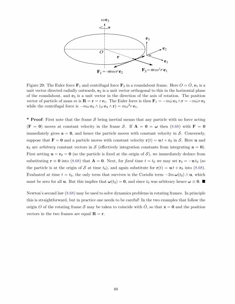
F
ω
3
rO
F1= -mωr
e3
e1
e2
e3
e2 =mω2r e1
Figure 29: The Euler force F1 and centrifugal force F3 in a roundabout frame. Here O = O, e1 is aunit vector directed radially outwards, e2 is a unit vector orthogonal to this in the horizontal planeof the roundabout, and e3 is a unit vector in the direction of the axis of rotation. The positionvector of particle of mass m is R = r = r e1. The Euler force is then F1 = −mω e3 ∧ r = −mωr e2
while the centrifugal force is −mω e3 ∧ (ω e3 ∧ r) = mω2r e1.
* Proof: First note that the frame S being inertial means that any particle with no force acting
(F = 0) moves at constant velocity in the frame S. If A = 0 = ω then (8.68) with F = 0
immediately gives a = 0, and hence the particle moves with constant velocity in S. Conversely,
suppose that F = 0 and a particle moves with constant velocity r(t) = u t+ r0 in S. Here u and
r0 are arbitrary constant vectors in S (effectively integration constants from integrating a = 0).
First setting u = r0 = 0 (so the particle is fixed at the origin of S), we immediately deduce from
substituting r ≡ 0 into (8.68) that A = 0. Next, for fixed time t = t0 we may set r0 = −u t0 (so
the particle is at the origin of S at time t0), and again substitute for r(t) = u t + r0 into (8.68).
Evaluated at time t = t0, the only term that survives is the Coriolis term −2mω(t0) ∧ u, which
must be zero for all u. But this implies that ω(t0) = 0, and since t0 was arbitrary hence ω ≡ 0. �
Newton’s second law (8.68) may be used to solve dynamics problems in rotating frames. In principle
this is straightforward, but in practice one needs to be careful! In the two examples that follow the
origin O of the rotating frame S may be taken to coincide with O, so that x = 0 and the position
vectors in the two frames are equal R = r.
88
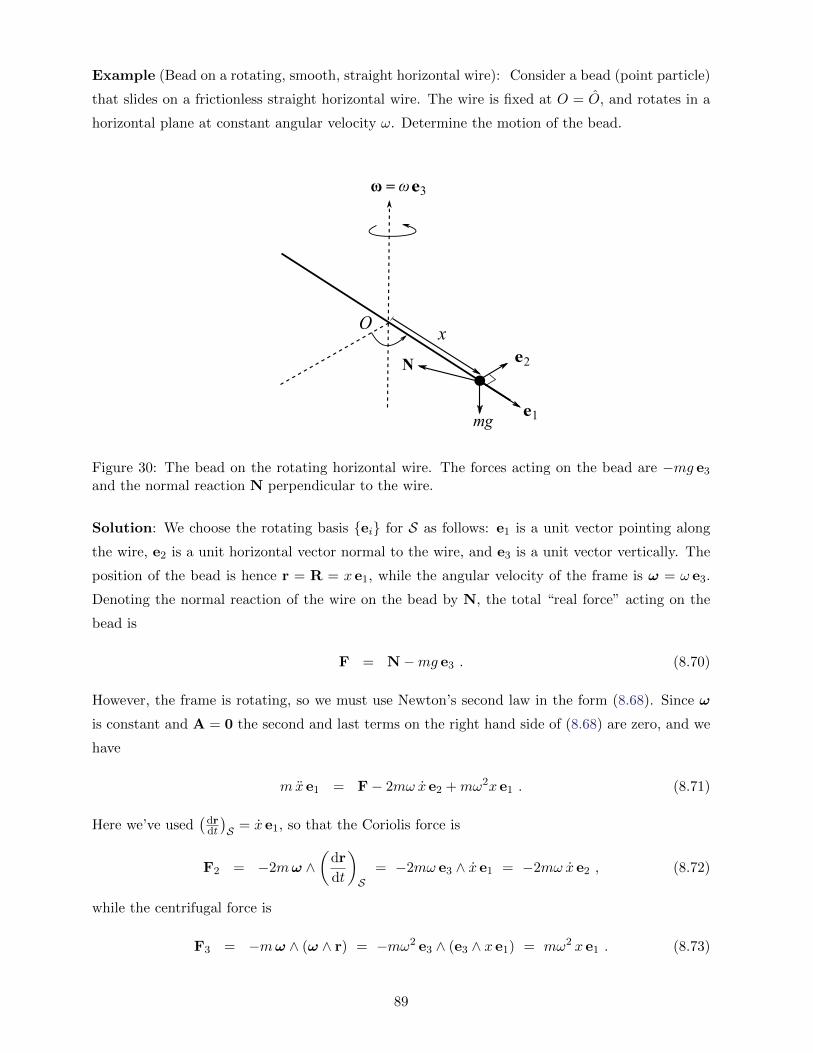
Example (Bead on a rotating, smooth, straight horizontal wire): Consider a bead (point particle)
that slides on a frictionless straight horizontal wire. The wire is fixed at O = O, and rotates in a
horizontal plane at constant angular velocity ω. Determine the motion of the bead.
Ox
ω = ωe3
mg
N
e1
e2
Figure 30: The bead on the rotating horizontal wire. The forces acting on the bead are −mg e3
and the normal reaction N perpendicular to the wire.
Solution: We choose the rotating basis {ei} for S as follows: e1 is a unit vector pointing along
the wire, e2 is a unit horizontal vector normal to the wire, and e3 is a unit vector vertically. The
position of the bead is hence r = R = x e1, while the angular velocity of the frame is ω = ω e3.
Denoting the normal reaction of the wire on the bead by N, the total “real force” acting on the
bead is
F = N−mg e3 . (8.70)
However, the frame is rotating, so we must use Newton’s second law in the form (8.68). Since ω
is constant and A = 0 the second and last terms on the right hand side of (8.68) are zero, and we
have
mx e1 = F− 2mω x e2 +mω2x e1 . (8.71)
Here we’ve used(
drdt
)S = x e1, so that the Coriolis force is
F2 = −2mω ∧(
dr
dt
)S
= −2mω e3 ∧ x e1 = −2mω x e2 , (8.72)
while the centrifugal force is
F3 = −mω ∧ (ω ∧ r) = −mω2 e3 ∧ (e3 ∧ x e1) = mω2 x e1 . (8.73)
89

As in section 5.1, the wire being smooth means that the normal reaction N has no component
along the wire, N · e1 = 0. Thus taking the dot product of (8.71) with e1 gives simply
mx = mω2 x . (8.74)
The general solution is
x(t) = A eωt +B e−ωt . (8.75)
For example, if the bead starts at a distance x = a from O with x = 0 at time t = 0, then
x(t) =a
2(eωt + e−ωt) = a coshωt . (8.76)
The bead hence flings outwards along the wire, with x(t) growing exponentially with t. �
Example (Bead on a rotating smooth hoop): A circular hoop of radius a rotates at constant
angular velocity ω about a vertical diameter. A bead slides smoothy on the hoop and has a position
vector which makes an angle ϕ with the vertical, as in Figure 31. Show that the equation of motion
is
ϕ+(ga− ω2 cosϕ
)sinϕ = 0 . (8.77)
O
ω = ωe3
mg
N
e1
e3
φ r
Figure 31: The bead on the rotating hoop. Here the figure shows the hoop at the instant at whichit passes through the plane of the page. The component N2 of the normal reaction N of the hoopon the bead points into the page at this instant, which is the e2 direction.
Solution: We take the origins O = O to be the centre of the hoop, and the frame S to be the rest
frame of the hoop. In particular we take e1 to be a horizontal unit vector and e3 to be a vertical
unit vector, which define the (rotating) plane of the hoop. We may then parametrize the position
of the bead as
r = R = a sinϕ e1 − a cosϕ e3 . (8.78)
90
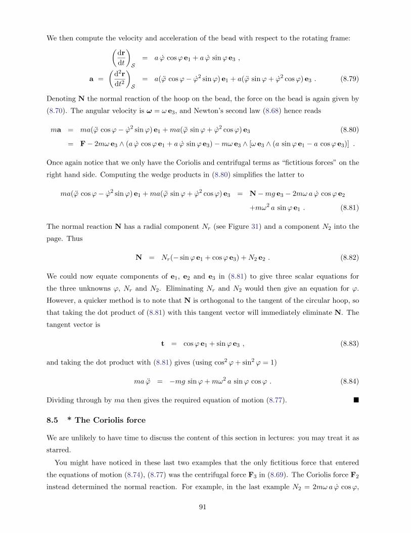
We then compute the velocity and acceleration of the bead with respect to the rotating frame:(dr
dt
)S
= a ϕ cosϕ e1 + a ϕ sinϕ e3 ,
a =
(d2r
dt2
)S
= a(ϕ cosϕ− ϕ2 sinϕ) e1 + a(ϕ sinϕ+ ϕ2 cosϕ) e3 . (8.79)
Denoting N the normal reaction of the hoop on the bead, the force on the bead is again given by
(8.70). The angular velocity is ω = ω e3, and Newton’s second law (8.68) hence reads
ma = ma(ϕ cosϕ− ϕ2 sinϕ) e1 +ma(ϕ sinϕ+ ϕ2 cosϕ) e3 (8.80)
= F− 2mω e3 ∧ (a ϕ cosϕ e1 + a ϕ sinϕ e3)−mω e3 ∧ [ω e3 ∧ (a sinϕ e1 − a cosϕ e3)] .
Once again notice that we only have the Coriolis and centrifugal terms as “fictitious forces” on the
right hand side. Computing the wedge products in (8.80) simplifies the latter to
ma(ϕ cosϕ− ϕ2 sinϕ) e1 +ma(ϕ sinϕ+ ϕ2 cosϕ) e3 = N−mg e3 − 2mω a ϕ cosϕ e2
+mω2 a sinϕ e1 . (8.81)
The normal reaction N has a radial component Nr (see Figure 31) and a component N2 into the
page. Thus
N = Nr(− sinϕ e1 + cosϕ e3) +N2 e2 . (8.82)
We could now equate components of e1, e2 and e3 in (8.81) to give three scalar equations for
the three unknowns ϕ, Nr and N2. Eliminating Nr and N2 would then give an equation for ϕ.
However, a quicker method is to note that N is orthogonal to the tangent of the circular hoop, so
that taking the dot product of (8.81) with this tangent vector will immediately eliminate N. The
tangent vector is
t = cosϕ e1 + sinϕ e3 , (8.83)
and taking the dot product with (8.81) gives (using cos2 ϕ+ sin2 ϕ = 1)
ma ϕ = −mg sinϕ+mω2 a sinϕ cosϕ . (8.84)
Dividing through by ma then gives the required equation of motion (8.77). �
8.5 * The Coriolis force
We are unlikely to have time to discuss the content of this section in lectures: you may treat it as
starred.
You might have noticed in these last two examples that the only fictitious force that entered
the equations of motion (8.74), (8.77) was the centrifugal force F3 in (8.69). The Coriolis force F2
instead determined the normal reaction. For example, in the last example N2 = 2mω a ϕ cosϕ,
91
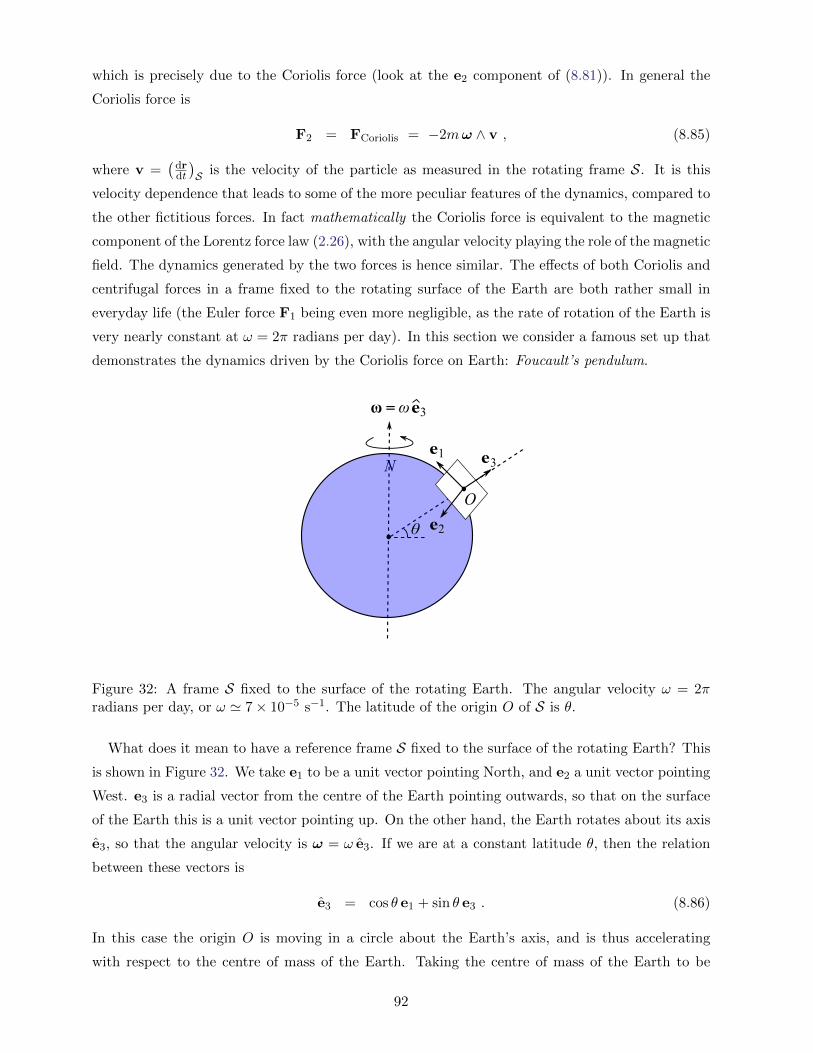
which is precisely due to the Coriolis force (look at the e2 component of (8.81)). In general the
Coriolis force is
F2 = FCoriolis = −2mω ∧ v , (8.85)
where v =(
drdt
)S is the velocity of the particle as measured in the rotating frame S. It is this
velocity dependence that leads to some of the more peculiar features of the dynamics, compared to
the other fictitious forces. In fact mathematically the Coriolis force is equivalent to the magnetic
component of the Lorentz force law (2.26), with the angular velocity playing the role of the magnetic
field. The dynamics generated by the two forces is hence similar. The effects of both Coriolis and
centrifugal forces in a frame fixed to the rotating surface of the Earth are both rather small in
everyday life (the Euler force F1 being even more negligible, as the rate of rotation of the Earth is
very nearly constant at ω = 2π radians per day). In this section we consider a famous set up that
demonstrates the dynamics driven by the Coriolis force on Earth: Foucault’s pendulum.
ω = ωe3
Ne1 e3
e2θ
O
Figure 32: A frame S fixed to the surface of the rotating Earth. The angular velocity ω = 2πradians per day, or ω ' 7× 10⁻⁵ s−1. The latitude of the origin O of S is θ.
What does it mean to have a reference frame S fixed to the surface of the rotating Earth? This
is shown in Figure 32. We take e1 to be a unit vector pointing North, and e2 a unit vector pointing
West. e3 is a radial vector from the centre of the Earth pointing outwards, so that on the surface
of the Earth this is a unit vector pointing up. On the other hand, the Earth rotates about its axis
e3, so that the angular velocity is ω = ω e3. If we are at a constant latitude θ, then the relation
between these vectors is
e3 = cos θ e1 + sin θ e3 . (8.86)
In this case the origin O is moving in a circle about the Earth’s axis, and is thus accelerating
with respect to the centre of mass of the Earth. Taking the centre of mass of the Earth to be
92
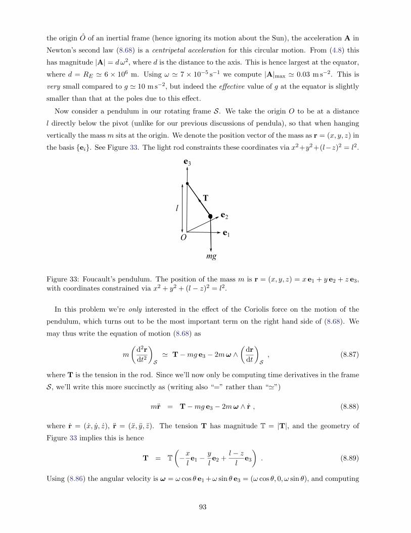
the origin O of an inertial frame (hence ignoring its motion about the Sun), the acceleration A in
Newton’s second law (8.68) is a centripetal acceleration for this circular motion. From (4.8) this
has magnitude |A| = dω2, where d is the distance to the axis. This is hence largest at the equator,
where d = RE ' 6 × 10⁶ m. Using ω ' 7 × 10⁻⁵ s−1 we compute |A|max ' 0.03 m s−2. This is
very small compared to g ' 10 m s−2, but indeed the effective value of g at the equator is slightly
smaller than that at the poles due to this effect.
Now consider a pendulum in our rotating frame S. We take the origin O to be at a distance
l directly below the pivot (unlike for our previous discussions of pendula), so that when hanging
vertically the mass m sits at the origin. We denote the position vector of the mass as r = (x, y, z) in
the basis {ei}. See Figure 33. The light rod constraints these coordinates via x2 +y2 +(l−z)2 = l2.
T
O
mg
l
e1
e2
e3
Figure 33: Foucault’s pendulum. The position of the mass m is r = (x, y, z) = x e1 + y e2 + z e3,with coordinates constrained via x2 + y2 + (l − z)2 = l2.
In this problem we’re only interested in the effect of the Coriolis force on the motion of the
pendulum, which turns out to be the most important term on the right hand side of (8.68). We
may thus write the equation of motion (8.68) as
m
(d2r
dt2
)S' T−mg e3 − 2mω ∧
(dr
dt
)S, (8.87)
where T is the tension in the rod. Since we’ll now only be computing time derivatives in the frame
S, we’ll write this more succinctly as (writing also “=” rather than “'”)
mr = T−mg e3 − 2mω ∧ r , (8.88)
where r = (x, y, z), r = (x, y, z). The tension T has magnitude T = |T|, and the geometry of
Figure 33 implies this is hence
T = T(−xle1 −
y
le2 +
l − zl
e3
). (8.89)
Using (8.86) the angular velocity is ω = ω cos θ e1 +ω sin θ e3 = (ω cos θ, 0, ω sin θ), and computing
93
the wedge product ω ∧ r the equation of motion (8.88) hence gives the following coupled ODEs
mx = −xlT + 2mω y sin θ ,
my = −ylT + 2mω(z cos θ − x sin θ) ,
mz =l − zl
T−mg − 2mω y cos θ . (8.90)
This is a complicated system, but let’s look at the equations for a very long pendulum, making
small oscillations. This means that the dimensionless quantities x/l and y/l are both small. On
the other hand, the constraint equation implies that (for z < l)
z
l= 1−
√1− x2
l2− y2
l2' x2
2l2+y2
2l2+ · · · . (8.91)
Thus z/l is second order in x/l, y/l, and we can hence take z/l ' 0 in this approximation. The
last equation in (8.90) then gives the tension as
T ' mg + 2mω y cos θ ' mg . (8.92)
Here the second approximation follows from the fact that ω ' 7×10⁻⁵ s−1 while g ' 10 m s−2: the
second term in T in (8.92) is the same order of magnitude as the first term if y ' 300, 000 miles
per hour! As in the example of a point charge moving in a constant magnetic field in section 2.4,
it is next useful to introduce the complex coordinate ζ = x+ iy. Using the approximations we’ve
made, the first two equations in (8.90) then become the real and imaginary parts of
ζ ' −glζ − 2ω sin θ i ζ . (8.93)
Compare this with (2.33) for a charged particle moving in a magnetic field. Substituting the ansatz
ζ = ept into (8.93) gives the quadratic equation
p2 + 2iω sin θ p+g
l= 0 , (8.94)
with roots
p = −iω sin θ ±√−ω2 sin2 θ − g
l= −iω sin θ ± i
√g
l
(1 +
ω2
g/lsin2 θ
)1/2
' −i
(ω sin θ ±
√g
l
). (8.95)
Again, the last approximation follows since ω2 is extremely small compared with g/l, for terrestrial
lengths l. The solutions may hence be written as
ζ(t) = x(t) + i y(t) ' e−iω sin θ t (C cos ω0 t+D sin ω0 t) , (8.96)
where C and D are complex integration constants, and ω0 =√g/l is the usual frequency of small
oscillations for the simple pendulum.
94
The term in brackets on the right hand side of (8.96) in general traces out an ellipse in the (x, y)
plane. Our usual simple pendulum confined to the (x, z) plane has C and D real, for which this
ellipse degenerates to a line. The phase e−iω sin θ t causes the ellipse to rotate in the (x, y) plane.
In the Northern hemisphere with θ > 0 this rotation is clockwise (viewed from above), while in
the Southern hemisphere with θ < 0 the rotation is anticlockwise. The period of the rotaton is
T = 24/| sin θ | hours, which is minimized at the North and South poles, θ = ±π2 .
Foucault built his original pendulum in 1851, in the Pantheon in Paris. It consisted of a 28 kg
metal bob with a 67 m long wire, suspended from the top of the dome. An exact replica has
been permanently swinging in the Pantheon since 1995 (apart from quite recently when repair
work was carried out). Paris has a latitude of θ ' 48◦, for which we calculate the period T ' 32
hours. Said differently, in a single day the pendulum motion has rotated through 270◦. Thus if the
simple pendulum starts swinging North–South (i.e. in a vertical plane), then at the same time the
following day it will be swinging East–West. This beautifully matches the (approximate) solution
we have found in this subsection.
The Coriolis force also plays an important role in the weather, for example being responsible for
the circulation of air around an area of low pressure, which is hence in the opposite directions in
the Northern and Southern hemispheres. That’s why the direction of spin of a hurricane depends
on whether it formed in the Northern or Southern hemisphere, and why hurricanes don’t form at
all near the equator at θ = 0. �
95