Dynamical energy analysis on mesh grids: a new tool

for describing the vibro-acoustic response of complex

mechanical structures

D.J. Chappella,∗, D. Lochelb, N. Søndergaardb, G. Tannerc

aSchool of Science and Technology, Nottingham Trent University, Nottingham NG118NS, UK

binuTech GmbH, Further Str. 212, 90429 Nurnberg, GermanycSchool of Mathematical Sciences, University of Nottingham, Nottingham NG7 2RD, UK

Abstract

We present a new approach for modelling noise and vibration in complex

mechanical structures in the mid-to-high frequency regime. It is based on a

dynamical energy analysis (DEA) formulation which extends standard tech-

niques such as statistical energy analysis (SEA) towards non-diffusive wave

fields. DEA takes into account the full directionality of the wave field and

makes sub-structuring obsolete. It can thus be implemented on mesh grids

commonly used, for example, in the finite element method (FEM). The result-

ing mesh based formulation of DEA can be implemented very efficiently using

discrete flow mapping (DFM) as detailed in [1] and described here for applica-

tions in vibro-acoustics. A mid-to-high frequency vibro-acoustic response can

be obtained over the whole modelled structure. Abrupt changes of material

parameter at interfaces are described in terms of reflection/transmission ma-

trices obtained by solving the wave equation locally. Two benchmark model

∗Corresponding authorEmail address: david.chappell@ntu.ac.uk (D.J. Chappell)

Preprint submitted to Wave Motion December 2, 2013

systems are considered: a double-hull structure used in the ship-building

industry and a cast aluminium shock tower from a Range Rover. We demon-

strate that DEA with DFM implementation can handle multi-mode wave

propagation effectively, taking into account mode conversion between shear,

pressure and bending waves at interfaces, and on curved surfaces.

Keywords: Statistical Energy Analysis, Ray Tracing, Transfer operators

1. Introduction

A vast range of numerical methods have been developed for solving noise

and vibration problems in mechanical structures. Popular tools include fi-

nite element methods, finite volume methods, boundary element methods

and various spectral methods. There are, however, basic limitations when

approximating the solutions of wave equations directly: the size of the as-

sociated linear system increases with decreasing wavelength and numerical

schemes become inefficient when the local wavelengths are orders of magni-

tude smaller than typical dimensions of the physical system. One therefore

moves to high frequency methods, such as ray tracing. However, tracking

rays including multiple reflections on boundaries can become cumbersome,

in particular on curved surfaces and when including mode conversion at in-

terfaces.

These problems can partly be circumvented by using statistical approaches.

Dividing the structure into a set of substructures and assuming diffuse wave

fields and quasi-equilibrium conditions in each of the resulting subsystems

leads to greatly simplified set of equations based only on coupling constants

between subsystems. This idea forms the basis of statistical energy analysis

2

(SEA) [2], which has found widespread applications in the automotive and

aviation industry, as well as in architectural acoustics. The disadvantage of

SEA is that the underlying assumptions are often hard to verify a-priori, or

are only justified when an additional averaging over equivalent subsystems

is considered. These shortcomings have been addressed by Langley [3] and

more recently by Le Bot [4, 5]. A computational tool based on a linear oper-

ator approach for propagating ray densities called dynamical energy analysis

(DEA) has been proposed in [6]. DEA systematically interpolates between

SEA and full ray tracing. The name points at the similarities with SEA but

stresses at the same time the importance of non-diffusive transport along

the ray dynamics. In particular, in DEA we have much more freedom in

sub-structuring the total system and variations of the energy density across

sub-structures can be resolved.

The implementation of DEA as presented in [6, 7] corresponds to a spec-

tral boundary integral method; the integral equations are expanded using or-

thogonal basis approximations and the resulting matrix equations are solved

for the coefficients of the basis expansion of the solution. In [8], it has been

shown that using a boundary element method for the spatial variable and

a basis function expansion in the momentum coordinate leads to efficiency

gains. In DEA, coupling between subsystems is described in terms of re-

flection/transmission matrices. These matrices are obtained by solving the

wave equation locally in the coupling region. The interfaces can be, for exam-

ple, line junctions between plates of different thickness or junctions between

plates and stiff components, where the local wavelength is of the same order

as the size of the component.

3

We will demonstrate that the method can be implemented efficiently on a

mesh with thousands of subelements including multi-mode wave propagation.

Due to the geometric simplicity of typical (planar) mesh elements, DEA can

be modified using the method of Discrete Flow Mapping (DFM) [1] which

gives rise to huge efficiency gains. DEA provides then detailed resolution of

the energy density variation throughout the structure under consideration.

The method is applied to benchmark problems provided by Germanischer

Lloyd (part of a double-hull structure of a large ship) [9] and Jaguar Land

Rover (cast aluminium shock tower of a Range Rover). In these examples,

mode mixing between in-plane and bending modes is incorporated.

2. Dynamical energy analysis – a brief overview

2.1. From ray tracing to flow equations - an operator formulation

We present a brief overview of the problem set-up and methodology, for

more details see [6, 7, 8, 10]. We consider linear wave problems driven by a

distribution of sources at a fixed angular frequency ω; a generalisation to fre-

quency band excitation is straightforward and is discussed below. The total

system is defined on a domain Ω, which is divided into a set of sub-domains

Ωj, j = 1, . . . , NΩ, such as the elements of a mesh grid. The material param-

eters and hence the local wave speeds are assumed to be constant in each

sub-domain, but may vary between sub-domains. Damping is incorporated

through a complex-valued damping term µ, which may depend on ω. In

general, one needs to determine the solution u of a wave equation (where u

is, for example, the displacement within a solid or pressure variations within

4

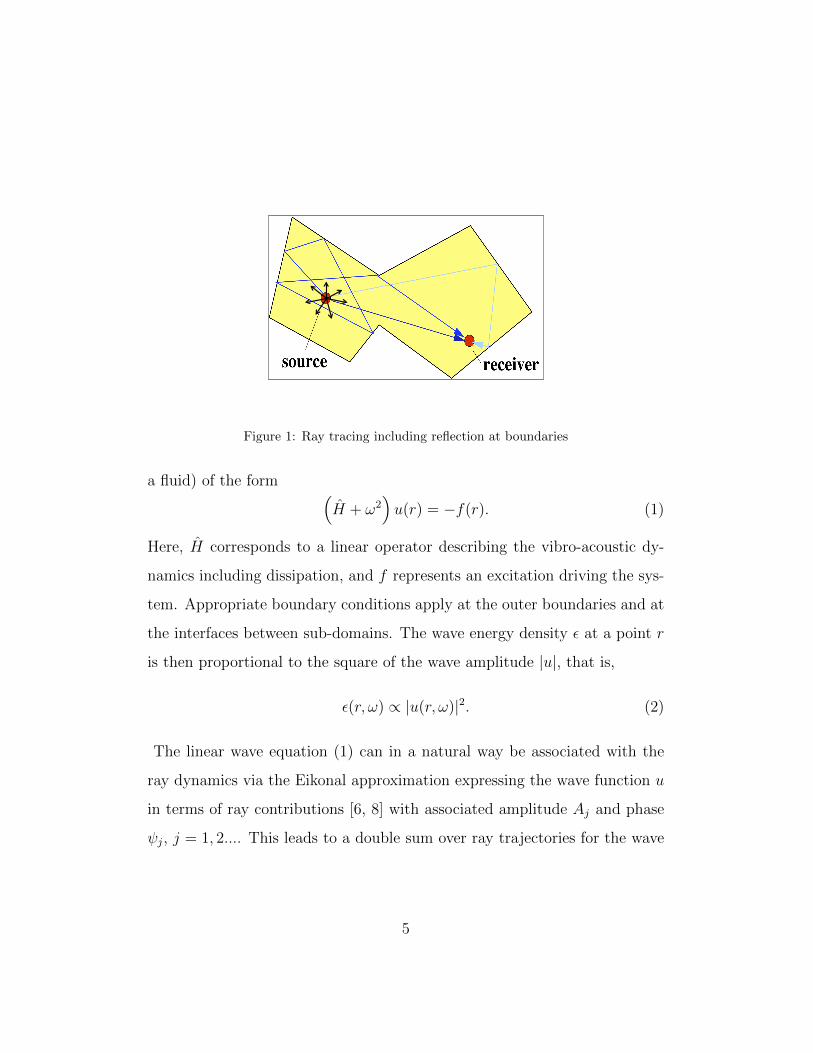
Figure 1: Ray tracing including reflection at boundaries

a fluid) of the form (H + ω2

)u(r) = −f(r). (1)

Here, H corresponds to a linear operator describing the vibro-acoustic dy-

namics including dissipation, and f represents an excitation driving the sys-

tem. Appropriate boundary conditions apply at the outer boundaries and at

the interfaces between sub-domains. The wave energy density ε at a point r

is then proportional to the square of the wave amplitude |u|, that is,

ε(r, ω) ∝ |u(r, ω)|2. (2)

The linear wave equation (1) can in a natural way be associated with the

ray dynamics via the Eikonal approximation expressing the wave function u

in terms of ray contributions [6, 8] with associated amplitude Aj and phase

ψj, j = 1, 2.... This leads to a double sum over ray trajectories for the wave

5

energy density of the form

ε(r, ω) ∝∑j,j′

Aj(r, ω)Aj′(r, ω) cos(ω(ψj(r)− ψj′(r)))

=∑j

Aj(r, ω)2 +∑j 6=j′

Aj(r, ω)Aj′(r, ω) cos(ω(ψj(r)− ψj′(r))).

(3)

Taking the average over a frequency band centered on ω0 such that the second

summation becomes negligibly small, then the mean wave energy density is

well approximated by the density of rays ρ(r, p, ω0) passing through a point

r, hence

ε(r, ω0) ∝∑j

Aj(r, ω0)2

=

∫ρ(r, p;ω0)dp,

(4)

where p is the direction (or momentum) vector, the magnitude of which is

related to the wavenumber. From hereon we consider problems with a fixed

frequency excitation, where this frequency must be interpreted as the centre

frequency ω0 of a band average. The system is excited by one or more point

sources from which rays emerge uniformly and undergo reflections at bound-

aries as well as absorption processes, see Fig. 1. It is therefore possible to

relate wave energy densities to classical flow equations and thus thermody-

namical concepts, which are at the heart of SEA and DEA treatments. Note

that different mode types such as shear, pressure or bending modes in plates

are treated as rays with different local wave speed. Mode coupling at bound-

aries or interfaces leads to mode-conversion of rays, that is, the classical flow

of rays will undergo ray-splitting. The conversion rates between rays corre-

sponding to different modes are related to the modulus square of the entries

6

of an interface scattering matrix. Likewise, the transmission/reflection prob-

abilities between sub-domains are given by the ratios of the outgoing normal

power fluxes to the incoming normal power flux at the interface, which can

again be obtained from the scattering matrix.

DEA is based on the observation that these flow equations for ray densities

can also be described using linear partial differential equations, namely the

phase space Liouville equation (LE) [8]. In order to solve the stationary

flow problem we rewrite the LE in boundary integral form; the boundary

can be the physical boundary of the system and/or the union of interfaces

between the sub-domains. Note that when implemented on a mesh grid,

the total boundary consists of the union of all mesh element boundaries.

For simplicity, let us first consider a single domain with boundary Γ. We

map the ray density emanating continuously from the source points onto the

boundary. The resulting boundary density is equivalent to a source density

on the boundary producing the same ray field in the interior as the original

source field after one reflection.

Ray densities ρ emanating from the boundary are transported to the next

intersection with the boundary by the operator B,

B[ρ](Xs) := w(Xs)ρ(ϕ−1(Xs)) =

∫w(Ys)δ(Xs − ϕ(Ys))ρ(Ys )dYs. (5)

Here Xs = (s, ps) (and Ys) represent phase-space coordinates on the bound-

ary, that is, s parameterises the boundary Γ and ps denotes the direction (or

momentum) component tangential to Γ at s. Also ϕ is the boundary map

(see fig. 2); it takes a ray from a boundary point s with tangential direction

component ps along the straight line path to the next intersection with the

boundary. Note that ϕ is invertible in convex (sub-) domains. The weight

7

Figure 2: Transfer of ray densities by the boundary map ϕ

function w(Xs) contains absorption factors as well as reflection/transmission

coefficients. The stationary density on the boundary induced by an initial

boundary distribution ρ0Γ(Xs) is then obtained using

ρΓ =∞∑n=0

Bn[ρ0Γ] = (I − B)−1[ρ0

Γ], (6)

where Bn contains trajectories undergoing n reflections at the boundary.

The density distribution in the interior region can then be obtained from the

boundary density ρΓ. One obtains the density (4) after projecting down onto

coordinate space.

Note that the treatment sketched above is formally equivalent to ray trac-

ing. A generalisation to multi-domain problems with sub-domains Ωj, j =

1, . . . , NΩ is straightforward by introducing a multi-domain boundary map

ϕij and weight function wij describing the flow from the boundary of domain

Ωi to the boundary of Ωj. The operator B is then constructed from the set

of inter-domain operators Bij.

8

2.2. A basis representation for the ray tracing operator B

In the following we restrict our discussion to two-dimensional problems,

an implementation for the three-dimensional case is described in [10]. In

order to evaluate (6), a finite dimensional approximation of the operator B

is constructed. We approximate the boundary density using basis functions.

For the spatial variable s, piecewise constant boundary element functions on

the (discretised) boundary are used [8, 10]. For the approximation in the

momentum argument we choose a Legendre polynomial basis. Note that in

two dimensions, the variable ps ∈ (−|p|, |p|) in general with |p| on the energy

surface defined through H(p, r) = ω20, where the Hamiltonian H is related to

the wave operator H in (1). We thus write ρΓ in the form

ρΓ(Xs) ≈ne∑α=1

N∑β=0

ρ(α,β)bα(s)Pβ(ps). (7)

Here, N is the order of the basis expansion, ne is the number of elements

in the boundary mesh, Pβ is a scaled Legendre polynomial of order β and

bα denotes the piecewise constant boundary element basis function. The

coefficient vector ρ(α,β) in (7) is labelled in terms of the multi-index (α, β).

The matrix approximation B of the ray tracing operator B is obtained by

writing (5) in a weak Galerkin form using the basis approximation (7) and the

orthonormal inner product for Legendre polynomials, see [8, 10] for details.

Legendre polynomials are chosen since they do not require periodicity for

convergence (cf. a Fourier basis) and are relatively simple to implement.

For these reasons the method directly extends to an hp - boundary element

method as described in [8].

Once the matrix B has been computed, the values of ρ(α,β) in (7) are

9

evaluated using (6) by solving

(I −B)ρ(α,β) = ρ0(α,β). (8)

Here the source coefficients ρ0(α,β) are obtained by projecting ρ0

Γ onto the

finite dimensional space spanned by the basis functions as described in [8].

An approximation for the density distribution ρΓ on the boundary is obtained

after substituting ρ(α,β) back into (7). This distribution is then mapped back

into the interior region and after projecting onto position space we obtain

an approximation for the energy density in (4), see [8] for details. Frequency

band calculations are obtained by sampling the results over the frequency

band considered.

Recall the splitting into sub-domains Ωj, j = 1, . . . , NΩ introduced ear-

lier. Each sub-domain represents one subsystem for each mode of wave

propagation. Coupling between subsystems will be treated as losses in one

subsystem and source terms in another. Typical subsystem interfaces are

surfaces between the mesh elements of a grid, which may give rise to reflec-

tion/transmission due to, for example, sudden changes in material param-

eters, local boundary conditions or curvature effects. Alternatively, a total

transmission of wave energy may occur, for example, when the transmission is

between two sub-domains within a homogeneous flat region. We describe the

full dynamics in terms of subsystem boundary operators Bij. Flow between

Ωi and Ωj is possible only if these sub-domains share a common boundary.

We introduce a weight function wij in (5), which contains (in addition to the

usual damping term) reflection and transmission coefficients characterising

the coupling between subsystems i and j at the interface. When restricting

the implementation to planar sub-domains of simple geometric shape such as

10

for triangulated surfaces, there is a very efficient way of evaluating the op-

erators Bij in terms of the so-called discrete flow mapping (DFM) technique

as described in [1].

Note that the reflection/transmission coefficients depend in general on the

angle of incidence of the incoming/outgoing wave and thus on the momentum

of the incoming/outgoing ray. In the case of total transmission, the angles

of incidence of the incoming and outgoing ray coincide and the transmission

coefficient is equal to one. DEA thus incorporates coherent, directed wave

transmission through interfaces. This is in contrast to SEA, which assumes

diffusive wave fields in each subsystem, that is, wave fields consisting of a

uniform superposition of waves from all directions. We will discuss the details

about the implementation of interface scattering matrices in a DEA approach

in Sec. 2.3. Representing the operator Bij in a basis function expansion

spanning all subsystems leads again to a matrix equation, see [7, 10].

2.3. Interface scattering matrices for plate junctions

Reflection/transmission coefficients are obtained by calculating interface

scattering matrices. We focus here on interfaces forming junctions between

plates of varying thickness, a setting which is relevant for the benchmark

problems discussed in Sec. 3. For DEA, we require local wave solutions taking

into account the angle dependence of the corresponding wave scattering. To

find the transmission/reflection coefficients of a set of plates being coupled

at a common interface (such as depicted in Fig. 3), we follow [11, 12]. In

particular, we consider the connection between plates as line junctions, that

is, the interior properties of the junction are not modelled and the mass and

moment of inertia are neglected.

11

Figure 3: A selection of plate junction configurations depicting an incoming ray at angle

φ (dashed blue line) and reflected/transmitted rays of the three mode types (solid lines).

Let us consider a line junction which couples n different plates, assuming

semi-infinite plates for simplicity. The boundary conditions at the line junc-

tion correspond to dynamic conditions involving stresses and moments, and

kinematic conditions for the displacement and rotation of all plates. To con-

struct the transmission coefficients we calculate the response of the system

with respect to excitation due to an incoming plane wave meeting the inter-

face at an angle φ (see fig. 3). The incoming wave has a fixed wavenumber

and a characteristic mode, that is, it is of bending (b), pressure (p) or shear

(s) type. The outgoing waves typically have components in all plates and are

a mixture of all mode types. An evanescent b mode is included to complete

the description. Thus, for each plate we have 4 unknown amplitudes for the

4 different wave types. Possible material differences between the plates can

lead to different wavenumbers in different plates. For a given forcing with

a particular incoming mode in a particular plate, we can solve for the un-

known modal coefficients in all plates. In practice, we find the transmission

probabilities directly by calculating the ratio of outgoing to incoming normal

12

power fluxes.

Fig. 4 shows transmission coefficients calculated with the method devel-

oped in [11], here for the T-joint in Fig. 3 with material properties described

in Sec. 3. In particular, we plot the individual transmission coefficients for a

bending mode excitation on the vertical plate in Fig. 3 (a). The coefficients

τ ijxy represent the transmission from a wave mode x in plate i to a mode y

in plate j with x, y = b, p, s and i, j = 1, 2, 3. The plates are numbered as

shown in Fig. 3(a), that is, 1 for the vertical plate containing the incident

ray, 2 for the horizontal plate and 3 for the other vertical plate. The plot

shows the dependence of the coefficients on the (cosine of the) angle φ of the

incoming ray to the interface. Fig. 4 shows in particular that there is little

mode mixing between bending and in-plane modes, and bending modes are

predominantly reflected at T-junctions.

In the next section we implement this theory for predicting interface re-

flection/transmission properties to model wave energy transport in test struc-

tures provided by Germanischer Lloyd and Jaguar Land Rover. The results

displayed in Fig. 4 are incorporated as part of the weight function w in the

finite dimensional approximation of the DEA kernel (5). We assume that the

transmission coefficients depend only on the incoming momentum ps via the

angle of incidence φ. The outgoing angle is given by Snell’s law taking into

account refraction due to differences in the wave speed across the interface.

13

Figure 4: Reflection/transmission coefficients at 200 Hz for a steel T-joint (see fig. 3a) with

thickness 8 mm across the two coplanar plates and 16 mm for the perpendicular plate. The

normal flux τ ijxy of the outgoing bending (y = b), pressure (y = p) and shear (y = s) modes

in each plate j = 1, 2, 3 is shown for an incoming bending wave (x = b) in plate i = 1. φ

denotes the angle between the incoming ray and the tangent to the plate boundary (see

fig. 3). The coefficients τ11bp and τ13bp were too small to be visible in the plot.

14

Figure 5: Germanischer Lloyd benchmark example with 40 bending point sources ran-

domly placed within a sub-domain. The plots show the DEA results for the energy density

of (a) the bending mode (including verification against FEM), (b) the pressure mode and

(c) the shear mode. Energies are displayed on a logarithmic scale, positions are given in

meters.

15

3. Numerical results

3.1. Double-hull structure

We apply the method to a stiffened double bottom test structure pro-

vided by Germanischer Lloyd [9] consisting of 8 mm steel plates with 200 mm

×16 mm stiffeners, see Fig. 5. The distance between the upper and lower

plates is 1.5 m and the distance between the side walls is 3 m. The following

material parameters for steel are used: Young’s modulus E = 2.1 · 1011 Pa,

Poisson ratio 0.3, and the material density is 7800 kg/m3. We furthermore

use hysteretic damping with a damping loss factor 0.03 for all three mode

types.

In order to compute the DEA kernel efficiently using DFM techniques,

the structure is divided along plate intersections into N = 212 rectangular

sub-domains as shown in Fig. 5. We further subdivide the boundary of

each sub-domain using a boundary mesh with element size 0.2 m or less.

In the momentum coordinate we employ an 8th order Legendre basis. The

transmission/reflection coefficients are obtained as discussed in Sec. 2.3 and

computed directly when evaluating the integrals in (5). Note that due to the

regularity of the test structure, we only need to consider the three different

types of line joints displayed in Fig. 3. Here the T-joints consist of stiffeners

and plates, where the stiffener has twice the thickness of the steel plates. The

structure is excited by a set of 40 randomly placed point sources acting on

the bending degrees of freedom at 200 Hz in the upper part of the structure,

see Fig. 5 (a).

It should be noted that since the in-plane modes have wavelengths of

the same order as the size of the plates, the ray approximation (4) is only

16

valid provided the average is over a wide enough frequency band to include

sufficiently many structural modes. The benchmark problem considered here

can at 200 Hz also be handled using FEM, see the lower subplots of Fig. 5

(a). For full ship structures, 200 Hz is already in the high frequency regime

and beyond the range that can be simulated using FEM due to the sheer size

of the structure.

The computation was done on a quad-core processor machine (Intel core

i5-2540M cpu 2.60 GHz) with a total computation time of 6.5 minutes. The

computation of the matrix coefficients in the 194 562×194 562 sparse matrix

with 309 434 904 nonzero entries took 3.5 minutes, solving the linear system

with Gauss-Seidel iteration took 2.5 minutes.

Fig. 5 shows the structure and the wave energy density in each of the

three modes on a logarithmic scale. The first two rows display (a) the energy

stored in the bending mode including the excitation region. The calculations

are verified against an FEM result over a frequency band centred on 200

Hz. The agreement is clearly very good, although oscillations on the scale

of the wavelength remain in the averaged FEM result that are not captured

by our ray model. The energy density in the pressure waves is shown in

(b) and the shear energy in (c). As expected, the energy density decreases

with the distance to the excitation points due to damping and most energy is

contained in the bending mode. However, there are also striking differences

in the behaviour shown for the different mode types. The damping in the

bending mode is stronger than for the in-plane modes. The transfer from

bending energy in the excited plate into pressure wave energy takes place

predominantly in the side walls. The energy distribution for the pressure

17

(p) waves is then surprisingly directional and is dominated by propagation

along the side walls in both the x and y directions (as depicted in Fig. 5). In

contrast, the bending and shear waves show more uniform behaviour without

strong preferential directionality.

3.2. Range Rover shock tower

We now consider the transport of high frequency wave energy in thin

shells. High frequency vibro-acoustic models based on an SEA treatment

will be unsuitable in these circumstances since complex geometrical features

are difficult to include in SEA; obtaining a subdivision of the model into

well separated subsystems is thus highly challenging for large moulded cast-

ings. DEA can overcome these problems since it can be easily applied in the

framework of existing grids for finite element models, requires no choice of

subsystem division and incorporates the full geometry and directionality of

the energy flow.

We consider the elements of a surface triangulation as our DEA sub-

domains. Here, the power of the DEA-method together with the DFM im-

plementation becomes obvious as we can immediately work with the meshes

provided by the manufacturer, here Jaguar Land Rover, to perform the calcu-

lations. Any pre-processing in terms of finding adequate subsystems becomes

obsolete. Applying thin shell theory [13], the rays travel along geodesics on

the curved surface (provided the radius of curvature is large compared to the

wavelength). Ray tracing along geodesics can be implemented on the trian-

gulated surface following [14] by choosing incoming angle equal to outgoing

angle at each interface (independent of the angle of intersection of the mesh

elements). To incorporate mode mixing and reflection effects in regions of

18

Figure 6: Energy density on a thin aluminium shell (Range Rover shock tower) estimated

using an averaged full wave finite element model (left) and a DEA model (right) for 3%

hysteretic damping.

strong curvature, we interpret the mesh elements (triangles) as a set of plane

plate segments intersecting at the mesh boundaries. The angle of intersection

enters into the computation of the scattering matrix giving rise to reflection,

transmission and mode conversion as described in Sec. 2.3. Note that the

need to deal with non-straight boundaries on the curved surface is avoided

by instead working with the triangulation where all boundaries are straight.

The right hand side of Fig. 6 shows the response of a thin moulded alu-

minium car component (shock tower of a Range Rover) to a point force

applied perpendicular to the surface using DEA. The results are compared

against a finite element simulation for the full wave model performed using

Nastran. In order to maintain a tractable model size for the finite element

simulation and to study frequency ranges of industrial interest, the compu-

tation is performed at frequencies between 8 kHz and 10 kHz. This approxi-

mately corresponds to a third of an octave band centered at 9 kHz. The full

19

wave kinetic energy is computed in Nastran using shell elements and aver-

aged over 41 evenly spaced frequencies spanning the prescribed range with a

typical hysteretic damping level of 3%. The Nastran grid contains 40 670 ele-

ments comprising a mix of piecewise linear triangles and quadrilaterals. The

DEA computation is performed on a much coarser mesh consisting of 11 623

triangles and a 6th order Legendre polynomial basis in direction space.

As would be expected one sees more oscillation in the full wave model.

The prediction of the overall energy flow with DEA is good both in the regions

of high and low curvature. In particular, it can be noted in both models that

high curvature regions act as barriers for the energy flow. Such geometric

features would be entirely absent from SEA-type models and represent a

major advance in the simulation of large-scale high frequency vibro-acoustics.

The computations in this section were performed with the same quad-core

processor machine as in the previous section in 15 minutes.

4. Conclusions

We have presented an approach for modelling the transport of wave en-

ergy through complex structures. The proposed method, DEA, interpolates

between SEA and ray tracing, taking account of the ray dynamics within

the structure and including reflection/transmission and mode conversion at

interfaces. Coupling coefficients for more complicated subsystem junctions,

such as junctions connecting several plates, have been calculated using a

scattering approach and then incorporated into the DEA framework. We

have shown that DEA can be implemented on existing mesh grids using the

DFM technique.

20

In particular, DEA was applied to a model vibrational energy distribu-

tions in a ship structure provided by Germanischer Lloyd and in a Range

Rover body part. Results for a system with several thousand sub-domains

and including all three wave modes in plates have been obtained in a com-

petitive computing time-scale of a few minutes. Large scale effects due to

non-diffusive wave transport were observed throughout. Our numerical re-

sults demonstrate the advantages of a DEA treatment compared to SEA.

Damping, directionality and curvature effects can all be modelled providing

a detailed analysis in each wave mode with high resolution across the entire

structure.

Acknowledgement

The authors wish to thank Christian Cabos and Mark Wilken from Ger-

manischer Lloyd, and Stephen Fisher from Jaguar Land Rover for providing

the benchmark problems and for helpful discussions. Support from the EU

(FP7 IAPP grant MIDEA) is also gratefully acknowledged.

[1] D.J. Chappell, G. Tanner, D. Lochel and N. Søndergaard, Discrete flow

mapping: Transport of ray densities on triangulated surfaces, Proc. R.

Soc. A, 469, 20130153, 2013.

[2] R. H. Lyon and R. G. DeJong, Theory and Application of statistical energy

analysis (2nd edn.). Butterworth-Heinemann, Boston MA, 1995.

[3] R. S. Langley, A wave intensity technique for the analysis of high fre-

quency vibrations, J. Sound. Vib. 159, 483–502, 1992.

21

[4] A. Le Bot and A. Bocquillet, Comparison of an integral equation on

energy and the ray-tracing technique for room acoustics, J. Acoust. Soc.

Am. 108, 1732-1740, 2000.

[5] A. Le Bot, Energy transfer for high frequencies in built-up structures, J.

Sound. Vib. 250, 247–275, 2002.

[6] G. Tanner, Dynamical energy analysis – Determining wave energy dis-

tributions in vibro-acoustical structures in the high-frequency regime, J.

Sound Vib. 320, 1023-1038, 2009.

[7] D. J. Chappell, S. Giani and G. Tanner, Dynamical energy analysis for

built-up acoustic systems at high frequencies , J. Acoust. Soc. Am., 130,

1420-1429, 2011.

[8] D. J. Chappell and G. Tanner, Solving the stationary Liouville Equation

via a Boundary Element Method, J. Comp. Phys. 234, 487-498, 2013.

[9] C. Cabos, H. G. Matthies, The Energy Finite Element Method Noise

FEM. in Proc. IUTAM Symp. Vib. Analysis of Structures with Uncer-

tainties, St Petersburg, 2009, Eds.: A. K. Belyaev and R. S. Langley,

IUTAM series 27 (Springer, Heidelberg, 2011).

[10] D.J. Chappell, S. Giani and G. Tanner, Boundary element dynamical

energy analysis: a versatile method for solving two or three dimensional

wave problems in the high frequency limit, J. Comp. Phys. 231, 6181-6191,

2012.

[11] R. S. Langley and K. H. Heron, Elastic wave transmission through

plate/beam junctions, J. Sound Vib. 143, 241-253, 1990.

22

[12] R. J. M. Craik, I. Bosmans, C. Cabos, K. H. Heron, E. Sarradj, J. A.

Steel and G. Vermeir, Structural transmission at line junctions: a bench-

marking exercise, J. Sound Vib. 272, 1086, 2004.

[13] A. N. Norris and D. A. Rebinsky, Membrane and Flexural Waves on

Thin Shells, ASME J. Vib. Acoust. 116, 457-467, 1994.

[14] R. Kimmel and J. A. Sethian, Computing geodesic paths on manifolds,

Proceedings of the National Academy of Sciences of the USA 95, 8431-

8435, 1998.

23