Dynamic Stability and Reform of Political Institutions

Roger Lagunoff∗

November, 2008

Abstract

When are political institutions stable? When do they tend toward reform? This paper examinesa model of dynamic, endogenous institutional change. I introduce a class of dynamic political gamesin which the political aggregation rules used at date t+1 are instrumental choices under rules at datet. A political rule is stable if it selects itself. A reform occurs when an alternative rule is selected.It turns out that the stability of a political rule depends on whether its choices are dynamicallyconsistent. For instance, simple majority rules can be shown to be dynamically consistent in manycommon environments where wealth-weighted voting rules are not. More generally, the result appliesto an extended class of political rules that incorporate private activities such as extra-legal protests,threats, or private investment. The model makes use of an interpretation of rules as “players” who canstrategically delegate future policy-making authority to different institutional types. The approachcan be viewed as a comprehensive way of understanding various explanations of institutional changeproposed in the literature. A parametric model of dynamic public goods provision gives an illustration.

JEL Codes: C73,D72, D74Key Words and Phrases: Endogenous political institutions, recursive, dynamic political games,reform, stability, dynamically consistent rules, forward and backward consistency, inessential.

∗Department of Economics, Georgetown University, Washington DC 20057 USA. 202 687-1510.lagunofr@georgetown.edu. http://www.georgetown.edu/lagunoff/lagunoff.htm . This project beganwhile the author visited Johns Hopkins University and the W. Allen Wallis Institute of Political Economy atthe University of Rochester. I am grateful for their hospitality. I also thank two anonymous referees, and DaronAcemoglu, Luca Anderlini, Jimmy Chan, Eddie Dekel, William Jack, Jim Jordan, Mark Stegeman, and seminarparticipants at Berkeley, Cal Tech, Georgetown, Penn State, Toronto, VPI, Yale, the Penn PIER Conference,and the Latin American and North American Winter Meetings of the Econometric Society for their helpfulcomments and suggestions on earlier drafts of this paper.

1

1 Introduction

Reforms of political institutions are common throughout history. They come in many varieties.For example, periodic expansions of voting rights occurred in governments of ancient Athens(700- 338BC), the Roman Republic (509BC-25AD), and most of Western Europe in the 19thand early 20th centuries.1 Medieval Venice (1032-1300) altered its voting rule by graduallylowering the required voting threshold from unanimity to a simple majority in its Citizens’Council. Nineteenth century Prussia, where votes were initially weighted by one’s wealth,eventually equalized the weights across all citizens. England and France changed the scope oftheir decision authority by privatizing common land during the 16th and 17th century enclosuremovement.2 The U.S. government, by contrast, increased its scope under the 16th Amendmentby legalizing federal income tax in 1913.

The objective of this study is to understand what underlies a change in political institu-tions over time. Specifically, which environments tend toward institutional stability? Whichenvironments admit change? What are the relevant forces that drive this change?

These questions are addressed in an infinite horizon setting in which political institutionsare endogenous. The model has three critical features. First, political institutions arise in arecursive social choice framework: a political rule in date t is a social choice correspondencethat aggregates preferences of the citizens at each date t to produce both a policy in date tand a future political rule for date t+ 1. Second, institutional choices are instrumental. Thatis, the political rules do not enter payoffs or technology directly. Third, institutional choice iswide and varied: the types of rules that can be chosen are not limited.

Admittedly, the social choice approach is abstract, far more so than, say, any particulargame-theoretic model of institutions. Its virtue is its flexibility. Social choice rules can generallycapture the most elemental attributes of a polity without being mired in or overly sensitive tothe fine details of political mechanisms. Questions of who participates; how are votes ultimatelycounted; what types of policy choices are admissible, can all be accommodated in the presentframework. This study demonstrates how the approach can offer a comprehensive way ofunderstanding various explanations of institutional change proposed in the literature.

The model is developed in two stages. First, a benchmark model posits that all decisionsoccur in the public sector. The model is then extended to account for private decisions thatare not explicitly part of the polity. The main results concern the stability and reform ofpolitical rules. A political rule is a social choice correspondence indexed by some parameterθt that summarizes the formal procedures for governance, e.g., election laws, voting eligibility,fiscal constitutions, and so on, that are in use at that date. A politically feasible strategy is anendogenous law of motion that maps the prevailing political rule θt in date t to a possibly newrule θt+1 for use in date t + 1. Politically feasible strategies are the “equilibria” of this model.

1See Fine (1983), Finer (1997), and Fleck and Hanssen (2003).2See MacFarlane (1978) and Dahlman (1980).

1

They are analogous to Subgame Perfect equilibria in the sense that the strategies must yieldimplementable social choices after any history.

By definition, a political rule θt admits reform whenever the politically feasible strategymaps θt to a different rule θt+1 6= θt. That is, next period’s political rule is chosen to bedifferent than the present one. A rule θt is stable whenever θt+1 = θt, i.e., no reform occurs.The main concern of this study is therefore whether and when a rule is stable, or alternatively,when does it admit reform?

To address this question, the present paper adopts an approach taken in a number of politico-economic models of policy dating back at least to Krusell, Quadrini, and Rıos-Rull (1997).3 Inthese models, policy outcomes are obtained by maximizing a time consistent social welfarefunction or aggregator. Because the political rule is identified by an aggregator at each date, apolitical rule can be re-interpreted as a “player” in a dynamic stochastic game. This player’s“preferences” are those of the aggregator. In the present model, the political rule at t + 1 isalso a choice variable, and so a reform entails a strategic delegation of authority from one typeof “rule-as-player” to another. Rules are therefore stable when the current type chooses not todelegate.

It turns out that the stability of such a rule can be characterized by its dynamic consistencyor lack thereof. A rule θt is said to satisfy forward dynamic consistency (FDC) if it is rationalizedby an aggregator in which the optimal choice of θt+1 in date t would remain optimal if thedecision were hypothetically made at the beginning of t + 1. In other words, the current rulewould not “change its mind” if called upon to make the decision in the future. The ruleθt satisfies backward dynamic consistency (BDC) if the hypothetical t + 1 choices are, in fact,optimal at t. A dynamically consistent rule is one that is both FDC and BDC. Theorem 1 assertsthat any dynamically consistent rule is stable, and any stable rule is forwardly dynamicallyconsistent (FDC). Because FDC and BDC coincide when the choice of political rule is unique,these notions provide an approximately complete characterization of stable political institutions.

In the paper, this notion is referred to as “rule-based dynamic consistency” in order todistinguish it from consistency of an individual’s preferences. Rule-based dynamic consistencyhas some similarities. Like individual consistency, rule based consistency concerns the conflictbetween a decision maker’s current and his future “self” in evaluating tradeoffs.

However, unlike individual consistency, rule-based consistency comes from the internal work-ings of a political system. A rule may be inconsistent (in the rule-based sense) even if all indi-vidual preferences are perfectly consistent. For example, wealth-weighted voting rules, i.e., rulesin which an individual’s vote is weighted by his wealth, are usually dynamically inconsistentin environments where wealth distribution changes through time. Hence, they admit reform.Why? The reason is straightforward. The identity of a pivotal voter under wealth weightedvoting is sensitive to natural changes in the wealth distribution over time. But when the iden-

3See the Literature Review in Section 5.

2

tity of the pivotal voter changes, a conflict arises in the preferences of the current and futurepivotal voters. So why does this translate into institutional change? Notice that the conflictbetween present and future pivotal voter all occurs under a fixed political rule θt. Hence, nom-inal political authority remains the same, while de facto authority changes. Consequently, thenominal delegation of authority from θt to θt+1 may be viewed as an attempt to limit a de factochange due to a change in the wealth distribution.

By contrast, under standard formulations of technical change, the simple Majority Votingrule is dynamically consistent, hence stable. The reason is that in these formulations, theorder statistics of the wealth distribution are preserved in expectation even as its higher ordermoments change. In other words, if one individual is currently richer than another, then onaverage he is expected to be richer tomorrow. Since simple majority voting typically dependsonly on the median (an order statistic), the identity of the pivotal voter is not expected tochange.

Hence, while both individual and rule based consistency concern the conflicts betweenpresent and future “self,” the latter also depends on subtleties of political aggregation. Inparticular, as the wealth-weighted voting example demonstrates, the stability of a political rulemay depend on the internal structure of the rule itself, even in the absence of private sectorinfluences. This contrasts with the current literature on dynamically endogenous institutions.That literature tends to focus on extra-legal protests, usurpations of power, or other activi-ties that are not directly part of the polity.4 For example, in an influential paper Acemogluand Robinson (2000) argue that expansions of the voting franchise were used by the 19thcentury European elite to “buy off” the threat of a peasant revolt. The rationale for reformthen comes from the fact that institutional change solves a commitment or credibility problemwhen a government’s policies can be undone by private behavior - in this case the peasants’threat. Similar rationales for change are found in Justman and Gradstein (1999), Acemogluand Robinson (2001, 2005), Lagunoff (2001), Gradstein (2003), Greif and Laitin (2004), Jackand Lagunoff (2006a,b), Cervellati, et. al. (2006), and Gradstein (2007).5

Even if the various “external threat” theories of institutional change are correct, rule-basedconsistency offers a comprehensive way of understanding them. To show this is so, the fullmodel incorporates arbitrary private activities such as those examined in the literature. Anequilibrium of this full model consists of politically feasible public sector strategies and SubgamePerfect private sector ones. Despite the addition of private sector activities, our main resultshows that the previous result extends to this environment. That is, when political aggregationencompasses both public and private decisions, dynamically consistent “extended rules” areshown to be stable, and stable rules are forwardly dynamically consistent (Theorem 2).

Returning to the “external threat” explanation of reform, the idea of rule-based consistencyadds to main two insights. First, it provides a concise characterization of the differing incentives

4One exception is Messner and Polborn (2004). See Section 5 for a further discussion.5This literature and related work is discussed in detail in Section 5.

3

of government at various points in time. For example, the Acemoglu and Robinson (2000)argument in which the franchise expansion ameliorates the threat of a peasant revolt may bere-interpreted as a failure of dynamic consistency of the extended aggregator. In the absence ofinstitutional change, the elite responds to the private sector threat under the assumption thatthe future elite does not. Hence, a conflict between present and future objectives arises.

Second, rule-based consistency shows that seemingly distinct explanation for reform are, infact, the same underlying explanation. For example, Acemoglu and Robinson (2000) explanationfor franchise expansion is sometimes contrasted with that of Lizzeri and Persico’s (2004) whoposit an “internal conflict” rationale for reform. In their model, political competition inducesover-investment in redistributive transfers relative to public goods. This over-investment is moresevere in a restricted voting franchise, and so franchise expansion is in some cases unanimouslypreferred among the elite. Though the Lizzeri-Persico model is static, there is, nevertheless,a tension between the extended rule’s “objectives” before and after the results of the politicalcompetition. The inefficiency might be mitigated if, for instance, citizens could commit tocontingent votes before the political competition begins. Hence, in both papers, private sectoractivities account for institutional reform only insofar as they induce dynamically inconsistentpolitical aggregation. We illustrate this phenomenon as well in an Example in Section 4.

Section 2 introduces the benchmark model. Section 3 contains the results of that modeland goes on to illustrate the main trade-offs involved in keeping or changing a political rulein a parametric example of public goods provision. Section 4 extends the model to privatesector decisions and revisits the parametric example with private decisions included. Section 5discusses the related literature in more detail, placing the present model in the context of thatliterature. Section 6 is an Appendix with the proofs of all the results.

2 The Benchmark Model

This Section introduces the benchmark model of a pure public sector economy. For now, weabstract away from all private sector behavior such as individuals’ savings, investment, or labordecisions. Hence, in this benchmark model, all relevant decisions are carried out in the publicsector. Though not realistic, this benchmark isolates some of the relevant features of a politicalinstitution in order to determine its stability. Private sector behavior is later introduced intothe model in Section 4.

To lay the groundwork for the model, an illustration of the social choice approach is intro-duced below. The approach is then extended to an infinite horizon dynamic game which admitsthe potential for continual changes in the political rule itself. Though the model developed hereis abstract, Section 3 illustrates the ideas in a concrete parametric model.

4

2.1 A Social Choice Illustration

Before proceeding with the model, consider first a simple static social choice “illustration” tofix ideas. Let I = 1, . . . , n denote a society of individuals, with n odd, and let P denotea set of possible collective decisions or policies. These policies may be tax rates, allocationsof public goods, or pork. Each citizen i ∈ I has payoff function vi : P → IR defined on thepolicy space. A standard social choice approach entails that policies are chosen from a socialchoice correspondence, C, that maps each preference profile (v1(·), . . . , vn(·)) (from a set of suchprofiles) to a subset of policies C(v1(·), . . . , vn(·)) ⊆ P .

This standard model can, in fact, be extended to allow for choice of the correspondenceitself. Let Θ be an index set. Each parameter θ ∈ Θ is identified with a distinct social choicecorrespondence C(·, θ). Hence, given an index θ and a profile (v1(·), . . . , vn(·)), a policy p ∈ Pis politically feasible if p ∈ C(v1(·), . . . , vn(·), θ).

The index θ is, in a sense, a political rule since it summarizes society’s aggregation process asdefined by the correspondence C(·, θ). The classic choice between “dictatorship” and “majori-tarian democracy,” for instance, may now be represented as a choice between two parameters,θD and θM . Parameter θD is defined by: p ∈ C(v1(·), . . . , vn(·), θD) if p maximizes vi for someindividual i (the “dictator”). θM is defined as: p ∈ C(v1(·), . . . , vn(·), θM) if p is undominatedby any alternative p in a simple majority vote. The problem in this static setup is: what ruledetermines the choice over these two rules? A dynamic model solves this problem by supposingthat the choice between θD and θM for date t always takes place at a prior date in accordancewith the rule in use at that time.

2.2 A Dynamic Extension of the Social Choice Model

From here on, all defined sets are assumed to be Borel measurable subsets of Euclidian spaces,and all feasible choice spaces (e.g., the space of feasible policies) are assumed to be compact.At each date t = 0, 1, 2, . . . society must collectively choose a policy pt ∈ P . Each citizen ihas a payoff in each date given by ui(ωt, pt) where ωt is a state variable drawn from a set,Ω. The state can include a citizen’s asset holdings or any stock of physical or human capitalthat affects the citizen’s payoffs. ui is assumed to be continuous and nonnegative. The stateevolves according to a Markov transition technology q with q(B| ωt, pt) the probability thatωt+1 belongs to the (Borel) set B ⊆ Ω given the current state ωt and current policy pt. Foreach such B, q(B|·) is continuous on Ω × P . A citizen’s discounted payoff over the course ofhis lifetime is:

Eq

[ ∞∑t=0

δt(1− δ) ui(ωt, pt )∣∣∣ ω0

](1)

where δ is the common discount factor, and the expectation Eq[·] is taken with respect toMarkov transition q. The expectation in (1) is assumed to be finite for any feasible sequence

5

of states and policy choices.

Extending the notation of the static model, let θt ∈ Θ denote the prevailing political ruleat date t. The collective decision faced by a society at date t under rule θt is the choice pair(pt, θt+1), i.e., the choice of current policy and subsequent political rule. The composite state,st = (ωt, θt), consists of the economic state and the political rule. The set of states is S = Ω×Θ.A history at date t is the list ht = ((s0, p0), . . . , (st−1, pt−1), st) which includes all past data upto that point in time as well as the current state st = (ωt, θt). An initial history is given byh0 = (s0, ∅). Let H denote the set of all histories at all dates.

Society’s endogenous choices are summarized by a public strategy, a pair of decision func-tions ψ and µ, defined as follows. Given a history ht ∈ H, ψ determines the chosen policypt = ψ(ht) while µ determines the political rule θt+1 = µ(ht) chosen for next period.6 The in-stitutional strategy µ is of particular interest since it describes an endogenous dynamic processof institutional change from current to future rules. Denote the sets of each type of strategy byΨ and M , respectively. After any history ht ∈ H, a public strategy (ψ, µ) ∈ Ψ ×M producesa public decision, (ψ(ht), µ(ht)) = (pt, θt+1) which determines today’s policy and tomorrow’spolitical rule for this society. Each citizen’s continuation payoff is expressed recursively as

Vi(ht; ψ, µ) = (1− δ) ui(ωt, ψ(ht) ) + δ Eq

[Vi(h

t+1; ψ, µ)∣∣∣ ht, ψ(ht), µ(ht)

](2)

In (2), µ matters only indirectly through the policy strategy ψ since ψ may vary with thecurrent and past θs.

Notice that Vi(ht; ψ, µ) is a payoff, i.e., a scalar. However, social choice rules are defined on

profiles of preference orderings rather than payoffs, and so we use the notation Vi(ht; ·), with

the “dot” used as a placeholder for a public strategy (ψ, µ), and connoting citizen i’s preferenceordering over all (ψ, µ) ∈ Ψ×M .

We now have all the tools to define social choice in the dynamic model. As in the staticmodel, a political rule θt is an index for a social choice correspondence C. The difference isthat now C maps to strategies rather than outcomes. Formally, (ψ, µ) ∈ C(V (ht; ·), st )expresses the idea that the strategy (ψ, µ) is a feasible social choice of the correspondenceC(·, st) under the preference profile V (ht; ·) ≡ (V1(h

t; ·), . . . Vn(ht; ·) ) following history ht.7

Notice that C varies with “economic” state ωt as well as the political rule θt. This is naturalif the aggregation procedure makes use of economic information such as wealth. However, Cis assumed to have no structural dependence on past history. Indirect dependence can arisethrough citizens’ preferences. The pair (C,Θ) is referred to as the class of political rules.

6Strictly speaking ψ and µ need not be “strategic” choices. They could arise, for instance, from a purelymechanical process. For much of the analysis, however, these will be explicit strategic choices of some “Player”and so I just label them as “strategies” from the start.

7Formally, C( V (ht; ·), st ) ⊂ Ψ×M is a cylinder set. What this means is that C( V (ht; ·), st ) is a set of(ψ, µ) such that (ψ(hτ ), µ(hτ )) can take on any value in P ×Θ if τ < t. In other words, there are no restrictionson public decisions prior to date t.

6

Suppose initially that this society could commit permanently to a fixed law of motionfor political rules and policies. In that case, the social decision occurs once at t = 0. Thesolution, a public strategy (ψ, µ), then induces a distribution over paths (p0, θ1), (p1, θ2), . . .,fully determined in advance. A “politically feasible strategy” in this sense would satisfy

(ψ, µ) ∈ C( V (h0; ·), s0 ) ∀h0 (3)

At this point the dynamic model extends the static model in a straightforward way. Of course,a commitment of this type is arguably impossible in any real society. The Expression (3) isnecessary but not sufficient for “political feasibility” in the recursive, “time consistent” sense. Inorder to satisfy the lack of strategic commitment, feasible strategies at date t must be consistentwith feasible strategies at date t+ 1. That is,

(ψ, µ) ∈ C( V (ht; ·), st ) ∀ht ∀t = 0, 1, . . . , (4)

A politically feasible strategy is therefore a strategy (ψ, µ) which satisfies (4). On occasion wewill look at politically feasible strategies (ψ, µ) that vary only with the current (Markov) statest = (ωt, θt). We refer to these as politically feasible Markov strategies (or just “Markov-feasiblestrategies” for short).

Political feasibility is analogous to Subgame Perfection since strategies must be politicallyfeasible at each date and after any history. To emphasize the link with Subgame Perfection,consider the special case of a “Libertarian” political rule in which public decisions mimic pri-vately chosen activities. Let P ⊂ IRn where pi is chosen directly by the corresponding citizeni each period. Now let Θ = θ where C(·, ω, θ) is the set of Nash equilibria in the subgamestarting from t. The set of politically feasible strategies in this case is precisely the set ofSubgame Perfect strategies of the n-player stochastic game. This “Libertarian” example alsoshows that the social choice approach is not at odds with a more traditional noncooperativegame approach. In the latter, each political rule could be modeled explicitly as a noncooper-ative game, with the choice being over noncooperative games in future periods. The problemis: how should these game(s) be modeled? While there are agreed upon canonical social choicerepresentations of voting, there are relatively few such games, perhaps because strategic modelsof politics are notoriously sensitive to minor details.8 Robust results in noncooperative politicalgame models are therefore hard to obtain. Consequently, this paper exploits a “detail free”approach that models basic properties of polities without specifying the fine details.

3 Stability versus Reform

Fix a class of political rules, (C,Θ). Recall that a history ht includes the current state st =(ωt, θt) as well as all past policies and states. Denote by ht(θt) a history in which the political

8Even in the more canonical endogenous candidate models of Besley and Coate (1997) and Osborne andSlivinsky (1996) there are reasonable and numerous, alternative specifications of how candidates could emerge.

7

rule at date t is θt ∈ Θ. Given an institutional strategy µ, a political rule θt ∈ Θ admitsinstitutional reform in µ if there exists a date t and a set of histories ht(θt) of positive measuresuch that µ(ht(θt)) 6= θt.

9 Alternatively, a rule θt is stable in µ if it does not admit reform, i.e,if µ(ht(θt)) = θt for almost every ht(θt).

This study poses the question: when do political rules admit reform? When are they stable?Our main result shows that this question can be reduced to one checking whether the aggregatorsatisfies a certain “dynamic consistency” property. To motivate the result, we first examine theissue in a parametric special case of the model.

3.1 A Simple Parametric Model

In this section, we explore a parametric special case of the model. We assume a politicalinstitution determines the level of taxes in order to fund a durable public good such as publicliteracy. The economic state is ωt = (Gt, yt), where yt = (y1t, . . . , ynt) with yit the wealth ofCitizen i at date t (e.g, a parcel of land). Wealth yit produces a one-to-one return each periodof yit. Gt is the stock of a durable public good at t. The public good in period t + 1 dependson tax revenues in period t. A tax pt is imposed on the yield from one’s wealth/land. Thereis no depreciation. The transition law for the public good is deterministic and is given byGt+1 = Gt + (pt

∑j yjt)

γ, 0 < γ < 1. Finally, each citizen’s stage payoff is a linear function ofhis after-tax returns and his use of the public good: ui = (1− pt)yit +Gt.

There are two possible institutional choices: θM and θW . The political rule θM is theMajority Rule, whereas θW is the “Wealth-as-Power Rule” in which each individual is allocateda number of votes proportional to his wealth. According to our definition in (4), a politicallyfeasible strategy is one that satisfies

(ψ, µ) ∈ C( V (ht(θk); ·), ωt, θk ) ∀ht(θk) ∀k = M,W, ∀t

Formally, what this means is that under the rule θM , for any alternative strategy (ψ, µ), theset of individuals that prefer (ψ, µ) are not a majority, i.e,

J ≡ i ∈ I : Vi(ht; ψ, µ) > Vi(h

t; ψ, µ)

satisfies |J | ≤ n/2. Whereas under θW , the same set J of individuals have lower aggregatewealth:

∑i∈J yi <

∑i/∈J yi.

10

9Positive measure here refers to the joint distribution on t-period histories induced by q, ψ and µ. Fixinginitial history h0 and rewriting history ht as ht = (h0, (ω1, . . . ωt), (θ1, . . . , θt), (p1, . . . , pt−1), the measure onhistories ht is defined by the product measure qt ⊗ 1µt ⊗ 1ψt−1 where 1· denotes the dirac measures on Θt

and P t respectively.10The theoretical properties of wealth-weighted rules are typically difficult to characterize. In a purely redis-

tributive environment, Jordan (2006) shows that outcomes of the Wealth-as-Power rule correspond to the coreof a cooperative game in which a blocking coalition’s feasible allocations are determined endogenously by thestatus quo allocation.

8

Case A. Fixed Wealth Distribution. Suppose first that the wealth distribution yt = (y1t, . . . , ynt)is fixed for all time, so that yt = y for all t. Order individual wealth holdings from poorestto richest: 0 ≤ y1 ≤ y2 ≤ · · · ≤ yn. Denote aggregate wealth by Y =

∑j yj. In this case,

it is straightforward to show that the most preferred policy of a citizen is invariant to timeand states: p∗i = min1, Ay−1/(1−γ)

i where A = ( γδ1−δ

Y γ)1/(1−γ) is a constant. Evidently, whenpreferred tax rates are interior, wealthier citizens prefer lower taxes.

Politically feasible strategies in each rule are as follows. Given θM , let mt denote the identityof the Majority-pivotal voter at date t. Voter mt corresponds to the citizen with the medianwealth endowment, i.e., mt = m = (n + 1)/2. The identity of this individual never changesover time. Consequently, the resulting policy is ψ(ω, θM) = min1, Ay−1/(1−γ)

m .

Under the Wealth-as-Power rule, the pivotal decision maker is also time invariant. A policy isfeasible under θW if it is the ideal policy of a voter, denoted by w, with the “median wealth” in aneconomy with yi identical voters of type i ∈ I. More precisely, this voter may be found as follows:Citizen w satisfies yw = maxyj :

∑nk=j yk ≥

∑i yi/2. The preferred policy for this individual

is p∗w = min1, Ay−1/(1−γ)w . The resulting policy then is ψ(ω, θW ) = min1, Ay−1/(1−γ)

w .

Proposition 1 In Case A, both θM and θW are stable.

Intuitively, each rule can be associated with a single, dynamically consistent decision maker - thepivotal citizen. The question becomes: would this individual ever delegate decision authority toa different individual whose preference over policy is different than his own? By the Principleof Unimprovability (e.g., Howard (1960)) the answer is no.

B. Differential Wealth Accumulation. Suppose that at t = 0 the initial wealth distribution isyi0 = yi where yi is the same as before. Recall that y1 ≤ · · · ≤ yn. Rather than remainingfixed, suppose that for t ≥ 1, yi t+1 = yit + βi with β > 0,

∑j βj = 1, and β1 < · · · < βn.

In this example, wealthier citizens accumulate wealth faster than poorer ones. One can checkthat each citizen’s most preferred policy is again of the form: p∗it = min1, Aty

−1/(1−γ)it where

At = ( γδ1−δ

Y γt )1/(1−γ) which now varies exogenously over time.

Under the differential accumulation rates, however, the two rules generally operate quitedifferently. Under the Majority Rule, the ordering of the wealth endowments never changes.Consequently, as before, the identity of the Majority-pivotal voter m never changes. Thisvoter’s wealth at date t is given by ymt. Hence, while the policy itself may change over timeaccording to ψ(ωt, θ

M) = min1, Aty−1/(1−γ)mt , the Majority-pivotal citizen has no incentive to

delegate decision authority to another. Therefore, the Majority rule remains stable.

By contrast, under the Wealth-as-Power rule, the identity of the pivotal voter may changeover time. This gives a potential rationale for institutional reform: a current decision makerwhose wealth is close to ymt may prefer the Majority-pivotal voter as a “lesser of two evils.”To illustrate this starkly, suppose that the parameters of the model are such that each citizen’s

9

preferred tax rate is always interior (strictly between zero and one). Suppose also that βn > 1/2.This inequality implies

ynt

Yt

=yn + tβn

Y + t∑

j βj

→ βn > 1/2

as t → ∞. In other words, the richest citizen eventually accumulates over half the aggregatewealth. Letting wt denote the sequence of pivotal decision makers under θW , the policy

strategy is given by ψ(ωt, θW ) = Aty

−1/(1−γ)wtt . It is clear that at some date t∗,

w0 ≤ w1 ≤ w2 ≤ · · · ≤ wt∗ = n

Now consider a sufficiently egalitarian initial wealth distribution. Specifically, suppose∑(n+1)/2

i=1 yi >Y/2. This implies that w0 = m. That is, the initial pivotal decision maker under θW is preciselythe Majority-pivotal (median) voter.

In this case, the institutional choice is made easy. Starting from θW , the Citizen w0 = m willchoose θM . Clearly, by remaining in θW , decision making authority is eventually transferredfrom the median citizen to the richest one. By choosing θM , however, this median citizenretains power. In the more general case where w0 6= m, this Citizen w0 may choose θM if hispreferences more closely resemble m’s over time than n’s. To summarize:

Proposition 2 In Case B, suppose an initial state ω0 = (y,G0) such that∑(n+1)/2

i=1 yi > Y/2.Then θM is stable, while θW admits reform. In particular, there exists some date t such thatµ(ht(θW )) = θM .

Since the preference of type m is strict, the Majority rule is preferred in all states in a neigh-borhood of ωτ . Hence, θW admits a reform toward θM .

The instability of θW owes to the fact that it varies in the economic state ωt. This leadsto change in the “identity” of the policy maker. If the shift is substantial enough, the currentdecision maker under θW may select an alternative political rule for self protection. Becausethe Majority Rule retains the same pivotal decision maker over time, no such self-protection isnecessary.11

3.2 A Baseline Result

The intuition of the parametric model demonstrates that a rule’s stability is closely alignedwith its tendency to “preserve a public decision maker’s identity” over time. Some parts ofthis statement need to be clarified. First, the idea of a rule’s “identity” must be defined. Weassociate a political rule with a social objective function or aggregator, whose maximal elements

11A related result is found in Messner and Polborn (2004) who use dynamic inconsistencies in the preferencesof the individual citizens. See Literature Review (Section 5) for more details.

10

are the outcomes of the rule. Formally, a class of rules (C,Θ) is rationalized by an aggregatorF : IRn

+ × S → IR+ if for any politically feasible strategy (ψ, µ),

(ψ(st), µ(st)) ∈ arg maxpt,θt+1

F((1− δ)u(ωt, pt ) + δEq[V (ht+1; ψ, µ) | ht, pt, θt+1], st

)(5)

An aggregator is a social welfare function that identifies a rule with a sequentially rational“player” whose payoff over public decisions each period is maximized by politically feasiblestrategies. It should be emphasized that this definition is unrestrictive: any class (C,Θ) isrationalized by a constant function.12

Having defined an aggregator F that rationalizes (C,Θ), we also need to be clear aboutwhat “preserving the aggregator’s identity” really means.

Definition 1 Let (C,Θ) be a class of political rules. Let F be an aggregator that rationalizes(C,Θ), and let (ψ, µ) be any public strategy. A rule θt is then said to be forwardly dynamicallyconsistent (FDC) if for all t, and every ht(θt),

arg maxθt+1

F((1− δ)u(ωt, ψ(ht(θt)) ) + δEq

[V (ht+1; ψ, µ) | ht(θt), ψ(ht(θt)), θt+1

], ωt, θt

)⊆ arg max

θt+1

Eq

[F

(V (ht+1; ψ, µ), ωt+1, θt

)| ht(θt), ψ(ht(θt)), θt+1

](6)

A rule is backwardly dynamically consistent (BDC) if (6) holds under the reverse inclusion, “⊇.”A rule is dynamically consistent if it is both FDC and BDC.

A rule θt is therefore FDC if any choice of rule θt+1 that maximizes F (·, ωt, θt) also maximizesthe expected continuation E[F (·, ωt+1, θt)]. A rule is BDC if the hypothetical maximizers ofE[F (·, ωt+1, θt)] also maximize F (·, ωt, θt). Significantly, this definition does not say anythingabout what the solution to either maximization problem should be.

Generally speaking, both forward and backward consistency capture the idea that, in theabsence of new information, such an individual should not “change his mind” about about adecision simply because the date at which the decision is made has changed. Alternatively,consistency can be formulated in terms of the value of commitment — a dynamically consistentdecision maker is one for whom there is no value of commitment.

Clearly, this is not a new idea. Individual consistency dates back at least to Howard (1960).Here, however, consistency is property of a rule rather than an individual. To make sense of

12One could therefore strengthen the definition in (5) so that (C,Θ) is fully rationalized by F means thepolitically feasible strategies coincide with (rather than contained in) the set of maximizers of F . This eliminatesthe degenerate cases, but it entails some loss of generality. Not every class of rules is fully rationalized by anaggregator. In any case, since the results do not depend on which definition is used, I opt for the weakerdefinition.

11

this, we interpret a rule θt as a “player” who delegates authority to some possibly different“player” θt+1 for next period. Hence, FDC states that, whatever political rule θt+1 happensto be chosen at date t, the aggregator F will not “change its mind” once the stage payoffsfrom period t have been realized. Similarly, BDC means if the aggregator were hypotheticallyallowed to choose θt+1 at the beginning of date t + 1 (before the new state is realized), thisaggregator would not “change its mind” if instead it could commit to a decision at date t.While neither FDC and BDC implies the other, in the important case where the maximizingsets in (6) are singletons (or, alternatively, both sets of maximizers are empty), then BDC andFDC coincide. We emphasize that while rule based consistency appears similar to individualconsistency, it ultimately comes from characteristics of political aggregation.

Before proceeding with the Theorem below, we have one final caveat: in order to excludeanswers that depend only on “ties,” define a conservative feasible strategy to be one in whichµ(ht(θ)) = θ whenever θ maximizes the aggregator F . In other words, θ avoids reform unlessthere is a strict incentive to change. “Ties” favor the status quo. Conservative strategies arisenaturally in any environment in which there is a small cost to changing the status quo.

Theorem 1 Let (C,Θ) be a class of political rules, and let F be an aggregator that rationalizes(C,Θ). For any conservative politically feasible strategy (ψ, µ), every dynamically consistentpolitical rule θt is stable, and every stable rule θt is forwardly dynamically consistent.

Heuristically, dynamic consistency ⇒ stability ⇒ FDC. Here, FDC is clearly the key concept.The proof in the Appendix is not deep. It extends the intuition of the Parametric model in astraightforward way. In Case A of that model, both θM and θW are dynamically consistent dueto the constant wealth distribution. However, in Case B the instability of the Wealth-is-PowerRule arises from a natural violation of FDC. Namely, θW varies in the economic state ωt. Thisleads to change in the “identity” of the public decision maker. Reform therefore occurs as ade jure response to a change in de facto power. Indeed, any political rule which depends oncardinal properties of a distribution of tastes or income is susceptible to nonlinear changes inthis distribution.

Consider the wealth-weighted voting rules such as θW . Though they have been widely usedhistorically, they are often short-lived. An example is 19th century Prussia. In 1849, votingrights were extended to most citizens in Prussia, but not in an even-handed way. Rights wereaccorded proportionately to the percentage of taxes paid. The electorate was divided intothirds, each third given equal weight in the voting. The wealthiest individuals who accountedfor the first third of taxes paid accounted for 3.5% of the population. The next wealthiest groupthat accounted for the middle third accounted for 10-12% of the population. The remainderaccounted for the remaining third. Following a growth spurt in the late 19th century, thewealth-weights were eliminated and a majority rule was adopted (see Finer (1997)).

Some final remarks conclude this Section. First, the model does not establish existence of

12

a politically feasible strategy. This issue is omitted in this paper, however, it is the subject ofa companion paper (Lagunoff 2006b).

Second, the Parametric Model illustrates only one source of inconsistency. There are others.A rule could, for instance, fail to be dynamic consistent if a particular citizen’s preferenceexhibits an inconsistency.13 It must be emphasized, however, that rule-based inconsistenciesare not dependent on individual inconsistencies.14 The particular source of inconsistency in theWealth-as-Power rule is a natural one arising from the rule’s reliance on a current economicstatus quo and from its over-sensitivity to subsequent changes in that status quo.

Third, in standard macro models featuring a social planner, the types of tradeoffs illustratedin the Parametric Model do not arise. An even stronger form of dynamic consistency is typicallypresumed. Namely:

F((1− δ)u(ωt, pt) + δEq

[V (ht+1; ψ, µ) | ωt, pt, θt+1

], st

)= (1− δ)F (u(ωt, pt), θt) + δ Eq

[F

(V (ht+1; ψ, µ), θt

)| ωt, pt, θt+1

] (7)

The expression (7) corresponds to the standard social planner’s problem according to whichF is linearly separable and does not directly vary in the economic states ωt. The ParametricModel illustrates how simple and common political rules violate the standard assumptions, and,consequently, will not last if the economic state changes in a natural way.

Finally, whether or not a particular rule is dynamically consistent can depend on Θ. Forinstance, if Θ = θM in the Parametric Model, then F is dynamically consistent, but expandingto Θ = θM , θW destroys consistency, as illustrated in the Model.15 Along the same lines,dynamic consistency can also depend on the class, though not necessarily the precise functionalform, of strategies under consideration. For example, a rule that is inconsistent under theMarkov strategies may well be consistent in a class of trigger strategies that makes full use ofthe history of the game. The latter can create consistent choices by means of self enforcingpunishments that sustain the desired outcomes.16 The link between consistency and the strategywill become more apparent when the polity must confront private actions of the citizens.

4 Private Sector Decisions

In the benchmark model, there are no private decisions of individuals; all decisions are madethrough the polity whose form depends on the political rule. One reason for considering private

13See, for instance, Krusell, Kuruscu, and Smith (2002) or Messner and Polborn (2004).14See Lagunoff (2006a) or Amador (2006) for models of dynamic inconsistencies arising from (exogenous)

electoral or dynastic changes.15I thank a referee for pointing this out.16See, for example, Dutta (1995) for a Folk Theorem for stochastic games.

13

or external decisions is that they are thought to be a driving force for institutional change in theliterature. Section 5 explores this literature in more detail. Whether or not this view is correct,this Section demonstrates that private decisions such as extra-legal protests, usurpations, laborand investments decisions, and so on, can be incorporated into an “extended political rule” towhich main result still applies.

Let eit denote i’s private decision at date t, chosen from a (compact) feasible set E. A profileof private decisions is et = (e1t, . . . , ent ). These decisions may capture any number of activities,including labor effort, savings, or investment activities. They may also include “non-economic”activities such as religious worship or one’s participation in a social revolt. The distinctionbetween eit and pt is that while the latter is collectively determined, the former is necessarilychosen individually. Yet, in the larger sense described below, the individual decisions just reflectconstraints on the overall social choice correspondence.

In keeping with the standard definition of a stochastic game, both private decisions et andthe public decision pt are made simultaneously. Clearly, there are sequential move alternatives,but none are clearly more compelling. In real time, private and public decisions are on-going.It seems natural then to define the dates as those intervals of time in which no agent is able topublicly pre-empt another.

Let ui(ωt, et, pt) and q(B| ωt, et, pt) denote the citizen stage payoff and transition probabil-ity, respectively. Both now depend on the profile of private actions as well as the public ones.All these components are summarized by a dynamic political game G given by:

G ≡ 〈economic primitives︷ ︸︸ ︷

(ui)i∈I , q, E, P,Ω ,

political rules︷ ︸︸ ︷C,Θ ,

initial state︷︸︸︷s0 〉.

4.1 Equilibrium and Extended Rules

A history at date t now includes the private action profiles, eτ , τ < t. A private strategy forindividual i is a history-contingent action, i.e., a function σi : H → Ei that prescribes actioneit = σi(h

t) after history ht. Let σ = (σ1, . . . , σn). A strategy profile is a list (σ, ψ, µ), whichincludes both private and public strategies. A citizen’s dynamic payoff may now be expressedas Vi(h

t; σ, ψ, µ). As before, V (ht; σ, ψ, µ) = (Vi(ht; σ, ψ, µ) )i∈I .

Definition 2 An Equilibrium of a dynamic political game G is a profile (σ, ψ, µ) of strategiessuch that for all histories ht ∈ H,

(a) Private rationality: For each citizen i, and each private strategy σi,

Vi(ht; σ, ψ, µ) ≥ Vi(h

t; σi, σ−i, ψ, µ ) (8)

14

(b) Political feasibility: Public strategies are politically feasible given σ:

(ψ, µ ) ∈ C(V (ht; σ, ·), st

)∀ht (9)

A Markov equilibrium is an equilibrium in Markov strategies. As before, equilibria, Markov orotherwise, satisfy a “subgame perfection” requirement.

Because the political rule (C,Θ) does not generally coincide with the interests of any privatedecision maker, it will not be the case that the public decision can be coordinated with anycitizen’s private one. Rather than carving out an exception, Definition 2 does not allow forcoordinated deviations between private and public decision makers even if they are one of thesame. While this restriction enlarges the equilibrium set, there is an obvious way to circumventthis issue by an appropriate reclassification of private decisions as public ones (along the lines ofthe “Libertarian” rule) whenever the public decision maker is one of the citizens. Indeed, evenwhen this is not the case, the map C can be extended to include private decisions. Formally,given any class of rules (C,Θ), an extended social choice map C∗ may be defined by

(σ, ψ, µ) ∈ C∗(V (ht, ·), st) ⇔

(ψ, µ) ∈ C(V (ht; σ, ·), st)

σi ∈ arg maxσi

Vi(ht; σi, σ−i, ψ, µ) ∀i

We refer to a political rule θ∗ associated with the extended class (C∗,Θ) as an extended politicalrule. Here, extended political rules incorporate private as well as public decisions.17 Theaggregator F ∗ is constructed so that it gives the same outcome as a “centralized” political systemthat would have occurred under in equilibrium under the “decentralized” political system inwhich public and private decisions are kept separate. F ∗ is therefore a “player” whose payoff ismaximized by an equilibrium (σ, ψ, µ). In this sense, we extend the rules-as-players approachdeveloped in the previous Sections extends in a straightforward way to the extended class(C∗,Θ).

4.2 A Theorem

For the remainder of the Section, fix a class (C,Θ) of political rules, and let (C∗,Θ) be theextended class. Let F ∗ be an aggregator which rationalizes (C∗,Θ).

Theorem 2 Let (σ, ψ, µ) be any conservative equilibrium. Then any dynamically consistentextended political rule θ∗ ∈ Θ is stable, and any stable extended rule θ∗ is forwardly dynamicallyconsistent.

17Although the extended rule θ∗ comes from the same index set Θ as before.

15

The proof has two steps. First, an appropriate relabeling of variables is required in order toapply the proof of Theorem 1. This involves taking private sector actions and appropriatingthem to the government or public sector. Private sector or individually chosen actions aretherefore part of a general social choice problem in which the social choice rule delegates decisionauthority over certain variables to the individual citizens. The second step repeats the steps ofthe Theorem 1 proof. We omit the details.

Despite the straightforward proof, the consequences are different from that of Theorem1 because the tension is between different agents rather than between different incarnationsof a political institution at different points in time. These consequences are illustrated in aparametric example below. The parametric structure is the same as before except that privatedecisions are included.

4.3 Adding a Private Sector to the Parametric Model

We revisit the parametric example, adding a private sector to the production of a public good.As before, the economic state is ωt = (Gt, y) with Gt a durable public good and y the wealthdistribution assumed here to be exogenous. Let 0 = y1 < · · · < yn. Given ε > 0 small, assumen is sufficiently large and the wealth distribution y “evenly distributed” in the sense that y1 < εand yj−yj−1 < ε. Now assume that each citizen can contribute labor effort eit at time t towardthe production of the public good. The transition is given by Gt+1 = Gt + (pt

∑j yj)

γ ∑j ejt

with 0 < γ < 1. Increased public literacy, for example, requires both public capital as givenby (pt

∑j yj)

γ and the sum of individual effort,∑

j ejt. Payoffs each period are defined byui = yi(1− pt) +Gt − e2it, now reflecting the cost or disutility of effort.18

Let (C,Θ) be a class of pivotal rules defined as those in which one of the citizens, say, citizeni with wealth yit is the dictator/pivotal voter. In that case, θt = yit . Given a state summarizedby st = (Gt, y, θt), a strategy (σ, ψ, µ) defines a law of motion over future states, e.g.,

st+1 = (Gt + (ψ(st)∑j

yj)γ

∑j

σjt(st), y, µ(st) ).

To find a closed form solution for an equilibrium, we restrict attention in the example toMarkov equilibria — equilibria in which strategies vary only with the state st. A citizen’s payoffmay then be expressed recursively by

Vi(st;σ, ψ, µ) = (1− δ)[yi(1− ψ(st)) +Gt − (σi(st))2] + δVi(st+1;σ, ψ, µ)

Since each political rule is dictatorial, the class of rules is alternatively rationalized by a simpleaggregator corresponding to the dictator’s payoff, .i.e.,

F (V (st; σ, ψ, µ), st) = (1−δ)[θt(1−ψ(st))+Gt−(σit(st))2]+δ F (V (st+1; σ, ψ, µ), st+1) (10)

18A similar example with ideologically heterogeneous agents is developed in Jack and Lagunoff (2006b).

16

-

6

45

µθ

θt = yiθt+1θt+2θt+3

Rule att+ 1

Political Rule at t

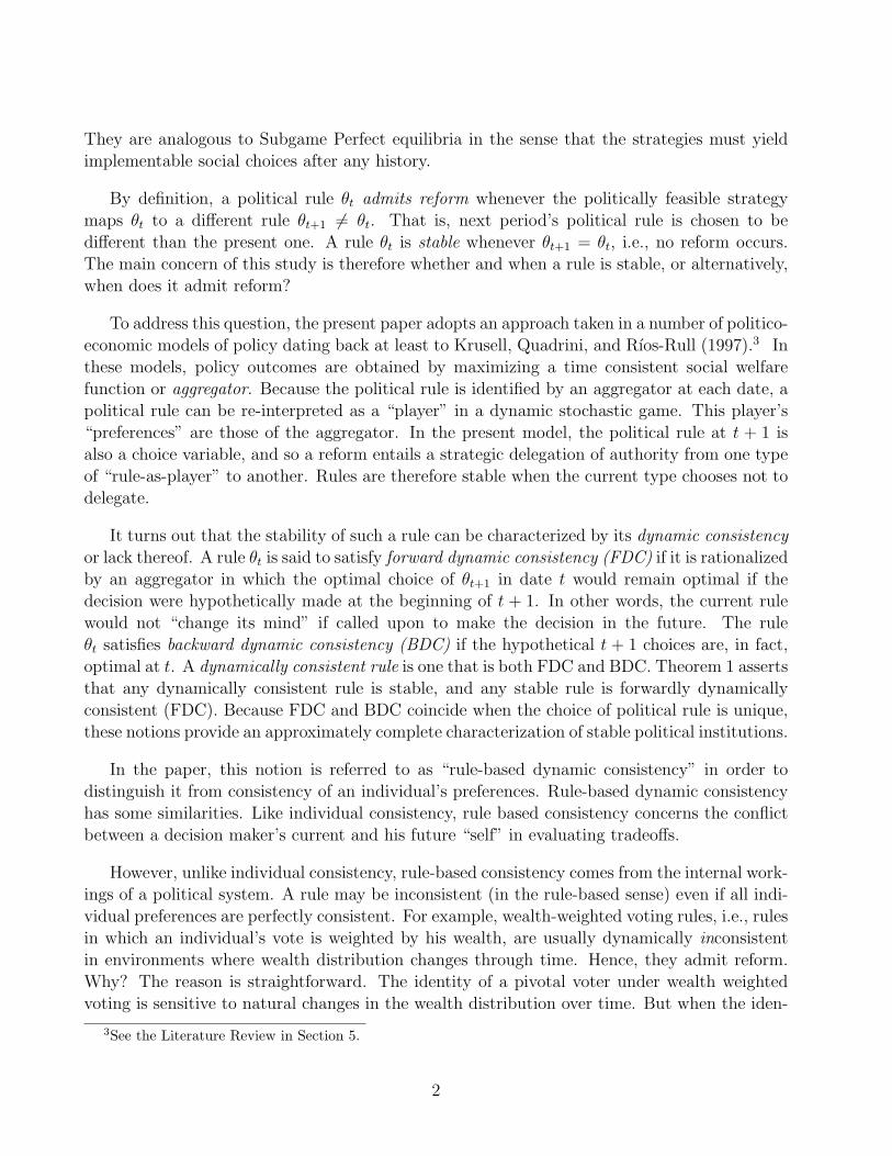
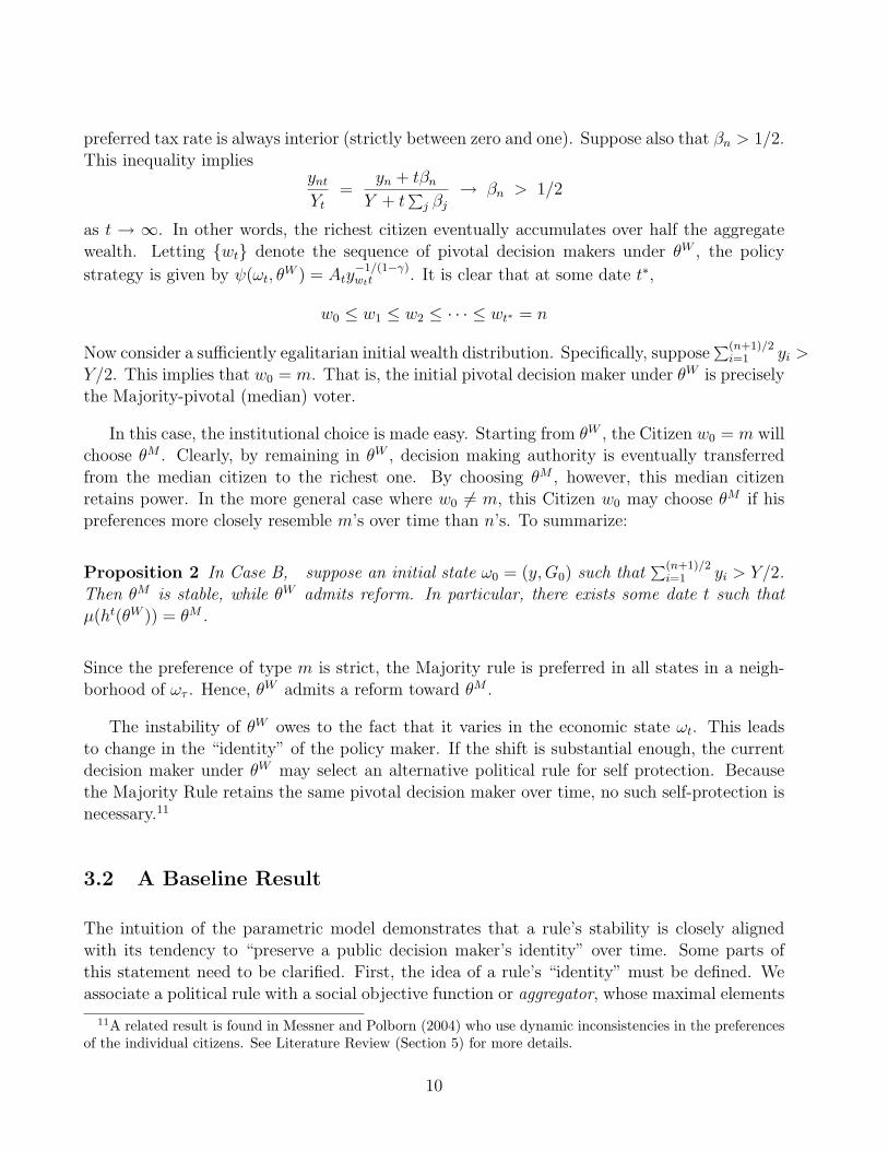
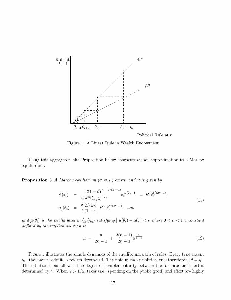
Figure 1: A Linear Rule in Wealth Endowment

Using this aggregator, the Proposition below characterizes an approximation to a Markovequilibrium.

Proposition 3 A Markov equilibrium (σ, ψ, µ) exists, and it is given by

ψ(θt) =2(1− δ)2

nγδ2(∑

j yj)2γ

1/(2γ−1)

θ1/(2γ−1)t ≡ B θ

1/(2γ−1)t ,

σj(θt) =δ(

∑j yj)

γ

2(1− δ)Bγ θ

γ/(2γ−1)t , and

(11)

and µ(θt) is the wealth level in yii∈I satisfying ||µ(θt)− µθt|| < ε where 0 < µ < 1 a constantdefined by the implicit solution to

µ =n

2n− 1+

δ(n− 1)

2n− 1µ

2γ2γ−1 (12)

Figure 1 illustrates the simple dynamics of the equilibrium path of rules. Every type excepty1 (the lowest) admits a reform downward. The unique stable political rule therefore is θ = y1.The intuition is as follows. The degree of complementarity between the tax rate and effort isdetermined by γ. When γ > 1/2, taxes (i.e., spending on the public good) and effort are highly

17

complementary and so effort is inefficiently high in equilibrium. On the other hand, whenγ < 1/2, the degree of complementarity is small, and so the free rider problem in private effortpredominates: effort is too low. In either case, the current dictator has an incentive to delegatefuture authority to an individual with lower wealth. When γ < 1/2, effort that is too low inequilibrium can be increased by transferring decision authority to a dictator from the lowerwealth strata. The transfer of power represents a commitment to a higher tax rate. Similarly,when γ > 1/2, excessively high effort can be reduced by the same such transfer, in this caserepresenting a commitment to a lower tax rate. In either case, the rich type cedes authority tothe poor type to gain more favorable private sector effort from the rest of the citizenry.

This private sector rationale seems quite different from the internal problems that createdinstability in the wealth-as-power rule in the previous example. Theorem 2, however, suggeststhat it is not. Consider what the extended aggregator would look like in this case. Let θ∗tdenote an extended rule, and let s∗t = (Gt, y, θ

∗t ). By reverse-engineering the equilibrium in

Proposition 3, the extended aggregator is derived as19

F ∗(V (s∗t ; σ, ψ, µ), s∗t ) = (1− δ)[θ∗t

n(1−ψ(s∗t )) +Gt−

∑j

(σj(s∗t ))

2] + δ F (V (st+1; σ, ψ, µ), st+1)

(13)Compare this F ∗ to F defined in (10). There are two main differences. First, the current stagepayoff in F ∗ eliminates the decentralization of, hence the free rider problem in, labor decisions.All citizens’ labor decisions are included, not just those of the dictator. Second, in order to“compensate” for the lack of a free rider problem, the current dictator’s wealth is now deflatedby 1

n(by assuming a type θ∗/n rather than θ∗). Intuitively, a wealthy dictator would like to

commit to act as if he were a poorer agent.

The key observation is that extended aggregator is adjusted so as to yield the same outcomethat would have been obtained in the decentralized model with private decisions. It does so byreformulating the decentralized problem as a centralized one with a dynamically inconsistentaggregator. Because the aggregator F ∗ has the same continuation as F but a different stagepayoff, it exhibits a dynamic inconsistency between objectives at date t and those of t+1. Thisinconsistency is not unlike that of hyperbolic models. The conflict is induced by the decisionmaker’s lack of direct control over private sector activities.

Consequently, Theorem 2 may be applied as follows to show that in a Markov equilibrium,the extended rule θ∗ = y1 is dynamically consistent (hence is stable) while every other extendedpolitical rule fails FDC (hence admits a reform). To see this, consider the extended class asgiven by (13), and substitute the Markov equilibrium in the Proposition in the definition of F ∗.Then dynamic consistency would imply that the solution set

arg maxθt+1

(1− δ)

θ∗tn

(1− ψ(θ∗t )) +Gt −∑j

(σj(θ∗t ))

2

+ δF (V (ωt+1, θt+1; σ, ψ, µ) (14)

19For a derivation, see the Appendix Proof to Proposition 3.

18

is equivalent to arg maxθt+1

F ∗(V (ωt+1, θt+1; σ, ψ, µ). In fact, this equivalence does not hold for all

extended rules except at the lower bound, θ∗ = y1.

5 Summary and Review of Literature

The idea of identifying a political institution with a time consistent social objective functionis not new. Krusell, Quadrini, and Rıos-Rull (1997), Hassler, et. al. (2005), and many othershave used it to model endogenous policy.20 The present paper builds on that idea by examiningthe choice of institution itself as a part of the aggregator’s objective. The model blends ideasfrom both social choice and stochastic games to produce a law of motion for political rules inwhich current rules select future ones. A stable rule is one that selects itself for use in thefuture. Stable rules can be understood in terms of a rule based dynamic consistency conceptthat identifies a rule with an aggregator.

This notion of self-selection bears some relation to “self-selected rules” in the static socialchoice models of Koray (2000) and Barbera and Jackson (2000), and also to the infinite regressmodel of endogenous choice of rules by Lagunoff (1992). These all posit social orderings onthe rules themselves based on the outcomes that these rules prescribe. Rules that “selectthemselves” do so on basis of selecting the same outcome as the original rule. The presentmodel has key two differences. First, institutional choice is explicitly dynamic. Second, thepresent model trades off economic fundamentals in the public and private sectors.

Apparently, the literature on explicitly dynamic models of endogenous political institutionsis sparse. There is a larger literature discussing the historical basis for modeling institutionalchange - see, for example, North (1981), Ostrom (1990), Grief and Laitin (2004), and theextensive political science literature discussed in Acemoglu and Robinson (2005). There is alsoa larger literature on static models of endogenous political rules. Examples include Conley andTemimi (2001), Aghion, Alesina, and Trebbi (2002), and Lizzeri and Persico (2004).

Among the dynamic models, a number of them concern the dynamic evolution of institutionsunder various exogenous rationales for reform. Roberts (1998, 1999) is an early example ofthis. He posits a dynamic delegation model as a way to understand progressive changes in asociety’s demographic composition. A pivotal voter in period t chooses a pivotal voter at datet + 1. In Robert’s model the attributes of a future voter appear directly in the preferencesof the current voter. A single crossing condition on the preferences guarantees that processof change is monotone or progressive from lower medians to higher ones. Because rules aredirect arguments of utility functions, the model is better suited to explain how, rather thanwhy, political institutions change.

Similarly, Justman and Gradstein (1999) examine endogenous voting rights under exogenous

20See Persson and Tabellini (2001) for other references.

19

costs of disenfranchisement. Barbera, Maschler, and Shalev (2001) examine club formationgames in which players have exogenous preferences over the size or composition of the group.As in Robert’s work, this “first wave” is ideally designed to study the process of, rather thanthe underlying rationale for, change.

The present paper bears a closer relation to a “second wave” of studies that attempt toput micro-foundations on the dynamics of institutional change. In this literature, institutionsare instrumental choices that arise from fundamental preferences over consumption and/ortechnological progress in economic tangibles. The additional step of obtaining robust andconvincing micro-foundations has proved difficult. Perhaps the most influential of these secondwave contributions are a series of papers by Acemoglu and Robinson (2000, 2001, 2005). Theypropose an instrumental theory to explain the process of democratization such as that whichoccurred in 19th century Western Europe. The 2000 paper posits a dynamic model in whichan elite must choose each period whether or not to expand the voting franchise to the restof the citizenry. The elite possesses the authority to tax but cannot commit to limit futuretaxes on the citizens. Because tax concessions alone cannot “buy off” the threat of an uprising,a more permanent commitment — namely an expansion of the voting franchise is required.The voting franchise is therefore expanded to head off social unrest. The timing of the reformdepends on, among other things, the likely success of an uprising in the absence of institutionalchange. Related ideas are found in Gradstein (2007) who models an elite’s choice of currentproperty protection as a commitment to future property rights, and in Cervellati, et. al. (2006)who model institutional choice in a game between competing social groups. Predatory conductdetermines the nature of the game — coordination or Prisoner’s dilemma — which, in turn,determines how successful the institutional move toward democracy will ultimately be. Jackand Lagunoff (2006a,b) go a step further by incorporating gradualism (as found, for instance, inRobert’s work) in an instrumental model of franchise expansion. Monotone rules of successionare derived when individuals differ by income, ideology, or both.

Though the following are not models of endogenous institutions per se, Powell (2004), Egorovand Sonin (2005), and Gomes and Jehiel (2005) all construct interesting dynamic games inthis spirit. Powell constructs a dynamic game in which a temporarily weak government maylack credibility to induce another government to restrain its inefficient use of power such aslaunching a coup or attacking. Egorov and Sonin construct a game in which a ruler’s powermay be usurped by a rival. The ruler can choose to kill a potential rival who constitutes a likelythreat. Finally, Gomes and Jehiel (2005) construct a institutional dynamic in which coalitionsform and unform over time, creating persistent inefficiencies along the way.

A somewhat different type of “instrumental institution” is modeled by Lagunoff (2001) whoformulates a dynamic game of endogenously chosen civil liberties. There, tolerant civil libertiesare chosen by a majority faction today in order to prevent a legal precedent for intolerancethat may be used against it by hostile majorities in the future. This self-reinforcing idea is alsofound in Grief and Laitin (2004) in which institutions are self enforcing outcomes in a repeatedgame.

20

The common thread in all these papers is that the impetus for change comes from theinability of a current polity to commit in advance to a future rule and thereby internalizethe social externalities created by private actions. A notable exception to this is the modelof Messner and Polborn (2004). In their model, institutional change is not driven by privateactions, but rather by dynamic inconsistencies in citizens’ preferences. They posit an OLGmodel in which current voting rules determine future ones. It is assumed that a citizen’s policypreference changes as he ages. However, the age distribution is assumed constant, and so apivotal voter today will be too old to remain pivotal tomorrow. For this reason, current rulestend to select more conservative (i.e., supermajority) rules in the future. As in the benchmarkmodel here, change is driven by a conflict between the present and future pivotal voters.

The present study is a step toward unifying the literature in the following sense. It re-interprets existing results as instances of a general phenomenon which can be understood with-out many stylized assumptions. Namely, that all reforms arise from some form of dynamicinconsistency in the extended aggregation process. Hence, the idea that progressive change inthe voting franchise occurs when a rule-by-oligarchic-elite is threatened by an external revoltcan be interpreted as an inconsistency between the present and future extended aggregationprocess. While the current extended payoff internalizes the peasants’ threat of uprising, theextended continuation does not. Consequently, delegation of authority occurs in order to inter-nalize the future threat.

Yet, the results are not specific to enfranchisement or any other particular type of insti-tutional reform. Nor is it the case that a reform requires an external threat of this type. Asthe Wealth-as-Power rule demonstrates, a reform can occur because common changes in theeconomic state can change the de facto distribution of power in a way that leads to institutionalchange.

It seems that the general link between an institution’s stability and its dynamic consis-tency has not, to my knowledge, been broadly understood. However, considerable caution iswarranted. As the last section (Section 4.3) suggests, the mapping between primitives and theextended rules is far from complete. Nor is it obvious that in all such cases, the re-interpretationby means of extended aggregation will be a useful one. These issues are focal points for futurework.

6 Appendix

To ease notation, we adopt the usual convention of using primes, e.g., θ′ to denote subsequentperiod’s variables, θt+1, with double primes, θ′′ for θt+2, and so on.

Proof of Theorem 1 Fix a politically feasible strategy (ψ, µ). Since this strategy is fixed forthe remainder of the proof we simplify notation by letting h denote a history consistent with

21

θ, i.e., h = h(θ). Also, define V ∗(h) ≡ V (h;ψ, µ).

We first show: if θ is dynamically consistent then θ is stable. Suppose, by contradictionthat θ is not stable. Then there is a set of h with positive measure such that for each such h,µ(h) = θ 6= θ. In that case,

θ ∈ arg maxθ′

F((1− δ)u(ω, ψ(h)) ) + δ

∫V ∗(h′(θ′))dq(ω′| ω, ψ(h) ), ω, θ

),

and, because (ψ, µ) is conservative, θ unstable implies,

F((1− δ)u(ω, ψ(h)) ) + δ

∫V ∗(h′(θ))dq(ω′| ω, ψ(h) ), ω, θ

)> F

((1− δ)u(ω, ψ(h)) ) + δ

∫V ∗(h′(θ))dq(ω′| ω, ψ(h) ), ω, θ

)By FDC,∫

F(V ∗(h′(θ)), ω′, θ

)dq(ω′| ω, ψ(h) ) ≥

∫F (V ∗(h′(θ)), ω′, θ) dq(ω′| ω, ψ(h) ) (15)

However, by BDC the inequality in (15) must be strict. Consequently, there is a set of ω′ withpositive measure such that

F(V ∗(h′(θ)), ω′, θ

)> F (V ∗(h′(θ)), ω′, θ) (16)

But by definition,

F (V ∗(h′(θ)), ω′, θ) = maxp′,θ′′

F((1− δ)u(ω′, p′) ) + δ

∫V ∗(h′′(θ′′))dq(ω′′| ω′, p′ ), ω′, θ

)

≥ F((1− δ)u(ω′, ψ(h′(θ))) ) + δ

∫V ∗(h′′(µ(ω′, θ)) ) dq(ω′′| ω′, ψ(h′(θ)) ), ω′, θ

)= F (V ∗(h′(θ)), ω′, θ)

which contradicts the inequality in (16).

Next, we show: if θ is stable then θ is FDC. By stability, µ(h) = θ a.e. By politicalfeasibility of (ψ, µ) it follows that

θ ∈ arg maxθF

((1− δ)u(ω, ψ(h) ) + δ

∫V ∗(h′(θ))dq(ω′| ω, ψ(h) ), ω, θ

)Suppose by way of contradiction, that θ is not FDC. Then

θ /∈ arg maxθ

∫F

(V ∗(h′(θ)), ω′, θ

)dq(ω′| ω, ψ(h) ) (17)

22

In that case there exists a θ 6= θ and a set of ω′ with positive measure such that

F(V ∗(h′(θ)), ω′, θ

)> F (V ∗(h′(θ)), ω′, θ) (18)

Notice that this does not automatically imply a contradiction because in (18) F is evaluatedunder next period’s state ω′ whereas one must show that stability is violated in the currentstate ω.

By the definition of feasibility, for all h′(θ),

F (V ∗(h′(θ)), ω′, θ) = maxp,θ

F((1− δ)u(ω′, p) ) + δ

∫V ∗(h′′(θ))dq(ω′′| ω′, p ), ω′, θ

)

≥ F((1− δ)u(ω′, ψ(h′(θ)) ) + δ

∫V ∗(h′′(µ(ω′, θ)) ) dq(ω′′| ω′, ψ(h′(θ)) ), ω′, θ

)= F

(V ∗(h′(θ)), ω′, θ

)(19)

Proof of Proposition 3.

We prove the second part of the Proposition — the explicit construction of a Markov equi-librium — first. Consider any Markov strategy (σ, ψ, µ) and any state st = (Gt, y, θt). Observefirst that the state enters linearly in the stage payoff. This means that a more convenient ex-pression of the recursive payoff function for a citizen can be derived by grouping the subsequentperiod’s state with the current stage payoff. Define Wi(θt; σ, ψ, µ) ≡ Vi(st;σ, ψ, µ) − Gt. Onecan show that the state variable in the right hand side of this equation cancels out. Conse-quently, Wi does not vary with Gt and can be expressed a function of θt alone. The aggregatorsF and F ∗ become

F (W (θt; σ, ψ, µ), θt) = (1− δ)[θt(1− ψ(θt)) + (ψ(θt)∑j

yj)γ

∑j

σjt(θt)− (σit(θt))2]

+ δ F (W (θt+1; σ, ψ, µ), θt+1), and

F ∗(W (θ∗t ; σ, ψ, µ), θ∗t ) = (1− δ)[θ∗tn

(1− ψ(θ∗t )) + (ψ(θ∗t )∑j

yj)γ

∑j

σjt(θ∗t )−

∑j

(σj(θ∗t ))

2]

+ δ F (W (θt+1; σ, ψ, µ), θt+1)

(20)respectively. Notice that the first order conditions under F with respect to p, and the first orderconditions of the Vj, j ∈ I with respect to ej all coincide with the joint first order conditionsin p and ej, j ∈ I under F ∗. In particular, Fixing θ = yi, the first order conditions in p andei, i ∈ I imply the policy and private sector strategies of the form in (11).

23

Since Wi does not depend on the economic state, then with strategies in (11), the recursivepayoff to citizen i is

Wi(θt; σ, ψ, µ) = (1− δ)[yi(1−B θ

1/(2γ−1)t ) + Aθ

2γ/(2γ−1)t

]+ δWi(θt+1; σ, ψ, µ) (21)

where A ≡ 14(2n− 1) δ2

(1−δ)2B2γ(

∑j yj)

2γ, a positive constant.

To find the approximate equilibrium institutional rule, µ, we guess and verify a linearapproximation θt+1 = µθt to the discrete solution. Using the equation for W in (21), theequilibrium continuation payoff is of the form

F ∗(W (θ∗t+1; σ, ψ, µ) = Wit+1(θt+1; σ, ψ, µ)

=∞∑

τ=t+1

(1− δ)δτ−t−1[yi(1−B (µτθt+1)

1/(2γ−1)) + A(µτθt+1)2γ/(2γ−1)

](22)

Clearly the set of θ∗t+1 that maximize (22) is nonempty since they come from the finite set,y1, . . . , yn. We obtain an approximation by taking first order conditions with respect to θt+1.Substituting for B and A, we verify that θ′ = µθ is an equilibrium for µ that satisfies (12). Itremains to show that a solution to (12) exists. To verify this final step, observe that as µ variesfrom 0 to 1, the left side (12) is continuously increasing from 0 to 1. Meanwhile, the right sideof (12) is continuously decreasing from n/(2n− 1) and approaches 0 asymptotically if γ < 1/2.If γ > 1/2, the right side of (12) is continuously increasing from n/(2n− 1) but has value lessthan one at µ = 1. In either case, Brouwer’s Theorem and the Intermediate Value Theoremimply a solution µ ∈ (0, 1) exists. Given that yj − yj−1 < ε, it follows that ||µ(θ)− µθ|| < ε.

References

[1] Acemoglu, D. and J. Robinson (2000), “Why Did the West Extend the Franchise? Democ-racy, Inequality and Growth in Historical Perspective,” Quarterly Journal of Economics,115: 1167-1199.

[2] Acemoglu, D. and J. Robinson (2001), “A Theory of Political Transitions,” AmericanEconomic Review, 91: 938-963.

[3] Acemoglu, D. and J. Robinson (2005), Economic Origins of Dictatorship and Democracy,book manuscript.

[4] Aghion, P., A. Alesina, and F. Trebbi (2002), “Endogenous Political Institutions,” mimeo.

[5] Amador, M. (2003), “A Political Model of Sovereign Debt Repayment,” mimeo, StanfordUniversty.

[6] Arrow, K. (1951), Social Choice and Individual Values, New York: John Wiley and Sons.

24

[7] Banks, J. and J. Duggan (2003), “A Social Choice Lemma on Voting over Lotteries withApplications to a Class of Dynamic Games,” mimeo, University of Rochester.

[8] Barbera, S. and M. Jackson (2000), “Choosing How to Choose: Self Stable Majority Rules,”mimeo.

[9] Barbera, S., M. Maschler, and S. Shalev (2001), “Voting for voters: A model of electoralevolution,” Games and Economic Behavior, 37: 40-78.

[10] Basar, J. and Olsder (1999), Dynamic Non-cooperative Game Theory, 2nd edition, Aca-demic Press, London/New York.

[11] Battaglini, M. and S. Coate (2005), “Inefficiency in Legislative Policy-Making: A DynamicAnalysis,” mimeo, July.

[12] Bernheim, D. and S. Nataraj (2002), “A Solution Concept for Majority Rule in DynamicSettings,” mimeo, Stanford University.

[13] Basar, J. and Olsder (1995), Dynamic Non-cooperative Game Theory, 2nd edition, Aca-demic Press, London/New York.

[14] Besley, T. and S. Coate (1997), ”An Economic Theory of Representative Democracy, Quar-terly Journal of Economics, 12:85-114.

[15] Conley, J. and A. Temimi (2001), ”Endogenous enfranchisement when Groups’ PreferencesConflict,” Journal of Political Economy, 109(1): 79-102.

[16] Black, D. (1958), The Theory of Committees and Elections, London: Cambridge UniversityPress.

[17] Blackwell (1965), “Discounted Dynamic Programming,” Annals of Mathematical Statistics,36:226-35.

[18] Cervellati, M, P. Fortunato, and U. Sunde (2006), “Consensual and Conflictual Democra-tization,” mimeo.

[19] Dahlman, C. (1980), The Open Field System and Beyond, Cambridge: Cambridge Univer-sity Press.

[20] Dutta, P. (1995), “A Folk Theorem for Stochastic Games,” Journal of Economic Theory,66: 1-32.

[21] Dutta, P. and R. Sundaram (1994), “The Equilibrium Existence Problem in GeneralMarkovian Games,” in Organizations with Incomplete Information: Essays in EconomicAnalysis, A Tribute to Roy Radner, M. Majumdar, ed., Cambridge: Cambridge UniversityPress, pp. 159-207.

[22] Egorov G. and K. Sonin (2005), “The Killing Game: Reputation and Knowledge in Non-Democratic Succession,” mimeo.

[23] Fine, J. (1983), The Ancient Greeks: A Critical History, Harvard University Press, Cam-bridge, MA.

[24] Finer, S.E. (1997), The History of Government, Oxford University Press, Oxford, UK.

25

[25] Fleck, R. and A. Hanssen (2003), “The Origins of Democracy: A Model with Applicationto Ancient Greece,” mimeo, Montana State University.

[26] Gans, J. and M. Smart (1996), “Majority voting with single-crossing preferences,” Journalof Public Economics, 59: 219-237.

[27] Gomes, A. and P. Jehiel (2005), “Dynamic Processes of Social and Economic Interactions:On the Persistence of Inefficiencies,” Journal of Political Economy, 113: 626667.

[28] Gradstein, M. and M. Justman (1999), “The Industrial Revolution, Political Transition,and the Subsequent Decline in Inequality in 19th Century Britain,” Exploration in Eco-nomic History, 36:109-27

[29] Gradstein, M. (2007), “Inequality, Democracy, and the Protection of Property Rights,”Economic Journal, forthcoming.

[30] Greif, A. and D. Laitin (2004), “A Theory of Endogenous Institutional Change,” AmericanPolitical Science Review, 98: 633-52.

[31] Hassler, J., P. Krusell, K. Storlesletten, and F. Zilibotti (2005), “The Dynamics of Gov-ernment,” Journal of Monetary Economics 52: 1331-1358.

[32] Howard, R. (1960), Dynamic Programming and Markov Processes, New York: M.I.T. andJohn Wiley and Sons.

[33] Jack, W. and R. Lagunoff (2006a), “Dynamic Enfranchisement,” Journal of Public Eco-nomics, 90: 551-572.

[34] Jack, W. and R. Lagunoff (2006b), “Social Conflict and Gradual Political Succession: AnIllustrative Model,” Scandinavian Journal of Economics, forthcoming.

[35] Jordan, J. (2006), “Pillage and Property,” Journal of Economic Theory, 131: 26-44.

[36] Kalandrakis, T. (2004), “A Three-Player Dynamic Majoritarian Bargaining Game,” Jour-nal of Economic Theory, 116: 294-322.

[37] Klein, P., P. Krusell, and J.-V. Rıos-Rull (2002), “Time Consistent Public Expenditures,”mimeo.

[38] Koray, S. (2000), “Self-Selective Social Choice Functions verify Arrow and Gibbard-Satterthwaite Theorems,” Econometrica, 68: 981-96.

[39] Krusell, P., V. Quadrini, and J.-V. Rıos -Rull (1997), “Politico-Economic Equilibrium andEconomic Growth,” Journal of Economic Dynamics and Control, 21: 243-72.

[40] Krusell, P., B. Kuruscu, and A. Smith (2002) “Equilibrium Welfare and Government Policywith Quasi-Geometric Discounting”, Journal of Economic Theory, 105.

[41] Lagunoff (1992), “Fully Endogenous Mechanism Selection on Finite Outcomes Sets,” Eco-nomic Theory, 2:465-80.

[42] Lagunoff, R. (2001), “A Theory of Constitutional Standards and Civil Liberties,” Reviewof Economic Studies, 68: 109-32.

[43] Lagunoff, R. (2006a), “Credible Communication in Dynastic Government,” Journal ofPublic Economics, 90: 59-86.

26

[44] Lagunoff (2006b) “Markov Equilibrium in Models of Dy-namic Endogenous political rules,” mimeo, Georgetown University,www.georgetown.edu/faculty/lagunofr/dynam-polit-b.pdf.

[45] Lizzeri, A., and N. Persico (2004), “Why did the Elites Extend the Suffrage? Democracyand the Scope of Government, with an Application to Britains Age of Reform, QuarterlyJournal of Economics, 119(2), 707-765.

[46] Osborne, M. and A. Slivinsky (1996), ”A Model of Political Competition with CitizenCandidates,” Quarterly Journal of Economics, 111:65-96.

[47] MacFarlane, A. (1978), The Origins of English Individualism, Oxford: Basil Blackwell.

[48] Mertens, J.-F. and T. Parthasarathy (1987), “Equilibria for Discounted Stochastic Games,”Core Discussion Paper 8750, Universite Catholique De Lovain.

[49] Messner, M. and M. Polborn (2004), “Voting on Majority Rules, Review of EconomicStudies, 71: 115-132.

[50] Montrucchio, L. (1987), “Lipschitz Continuous Policy Functions for Strongly Concave Op-timization Problems, Journal of Mathematical Economics, 16:259-73.

[51] North, D. (1981), Structure and Change in Economic History, New York: Norton.

[52] Osborne, M. and A. Slivinsky (1996), ”A Model of Political Competition with CitizenCandidates,” Quarterly Journal of Economics, 111:65-96.

[53] Ostrom, E. (1990), Governing the Commons: The Evolution of Institutions of CollectiveAction, Tucson: University of Arizona Press.

[54] Persson, T. and G. Tabellini (2002), Political Economics, Cambridge, MA: MIT Press.

[55] Powell, R. (2004), “The Inefficient Use of Power: Costly Conflict with Complete Informa-tion,” American Political Science Review, 98: 231-41.

[56] Roberts, K. (1977), “Voting over Income Tax Schedules,” Journal of Public Economics, 8:329-40.

[57] Roberts, K. (1998), “Dynamic Voting in Clubs,” mimeo, STICERD/Theoretical EconomicsDiscussion Paper, LSE.

[58] Roberts, K. (1999), “Voting in Organizations and Endogenous Hysteresis,” mimeo, NuffieldCollege, Oxford.

[59] Rothstein, P. (1990), “Order Restricted Preferences and Majority Rule,” Social Choice andWelfare, 7: 331-42.

27