Embed Size (px)
Citation preview

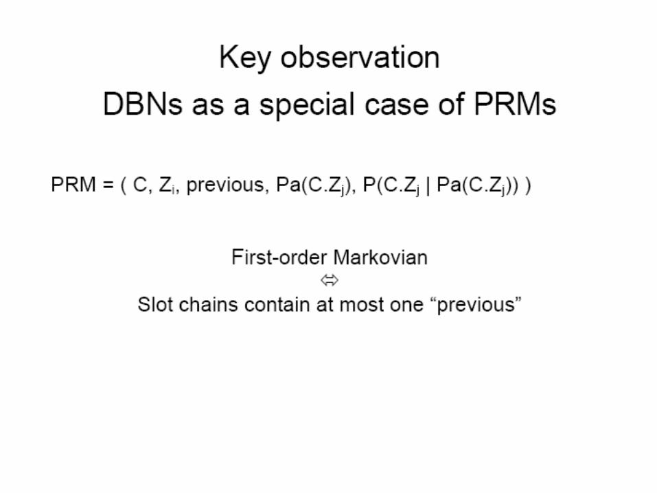
Dynamic Probabilistic Relational Models
Paper by: Sumit Sanghai, Pedro Domingos, Daniel Weld
Anna Yershova
Presentation slides are adapted from: Lise Getoor, Eyal Amir and Pedro Domingos slides
The problem
How to represent/model uncertain sequential phenomena?
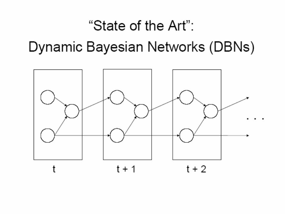

Limitations of the DBNs
How to represent: • Classes of objects and multiple instances of a
class • Multiple kinds of relations • Relations evolving over time
Example: Early fault detection in manufacturing Complex and diverse relations evolving over the manufacturing process.

PLATE
weightshapecolor
PLATE
weightshapecolor
PLATE
weightshapecolor
Fault detection in manufacturing
PLATE
weightshapecolor
PLATE
weightshapecolor
BRACKETweightshapecolor
welded tobolt
PLATE
weightshapecolor
PLATE
weightshapecolor
PLATE
weightshapecolor
BOLTweightsizetype
welded tobolt
PLATEweightshapecolor
welded tobolt
PLATE
weightshapecolor
PLATE
weightshapecolor
PLATE
weightshapecolor
ACTION
action


Strain s1
Patient p1
Patient p2
Contactc3
Contactc2
Contactc1
Strain s2
Patient p3
Strain
Patient
Contact
DPRM with AU Semantics
)).(|.(),S,|( ,.
AxparentsAxPP Sx Ax
I
AttributesObjects
probability distribution over completions I:
2TPRM relational skeletons 12+ =
Strain
Patient
Contact
Strain s1
Patient p1
Patient p2
Contactc3
Contactc2
Contactc1
Strain s2
Patient p3
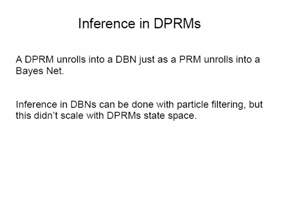

Particle Filtering
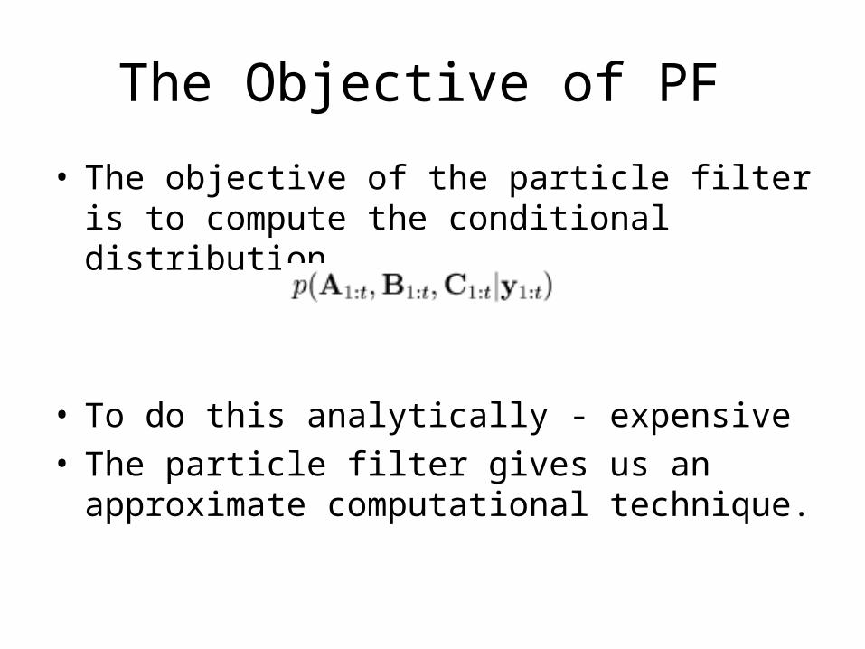
The Objective of PF
• The objective of the particle filter is to compute the conditional distribution
• To do this analytically - expensive• The particle filter gives us an approximate
computational technique.
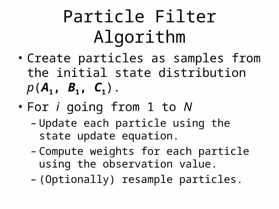
Particle Filter Algorithm
• Create particles as samples from the initial state distribution p(A1, B1, C1).
• For i going from 1 to N– Update each particle using the state update
equation.– Compute weights for each particle using the
observation value.– (Optionally) resample particles.
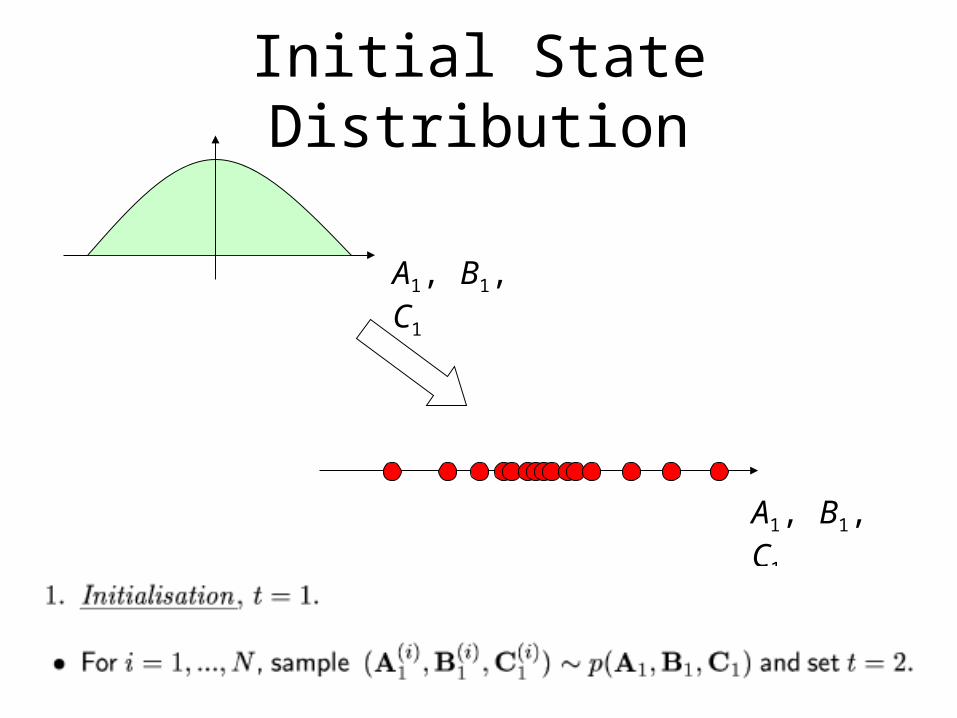
Initial State Distribution
A1, B1, C1
A1, B1, C1

Prediction
At, Bt, Ct
At, Bt, Ct = f (At, Bt, Ct )
At, Bt, Ct

Compute Weights
Before
After
At, Bt, Ct
At, Bt, Ct
At, Bt, Ct

Resample
At, Bt, Ct
At, Bt, Ct

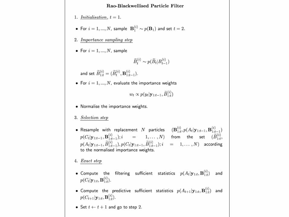

Rao-Blackwellised PF

Another Issue
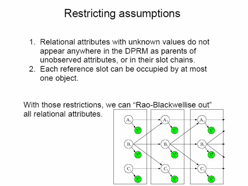
• Rao-Blackwellising the relational attributes can vastly reduce the size of the state space.
• If the relational skeleton contains a large number of objects and relations, storing and updating all the requisite probabilities can still become quite expensive.
• Use some particular knowledge of the domain
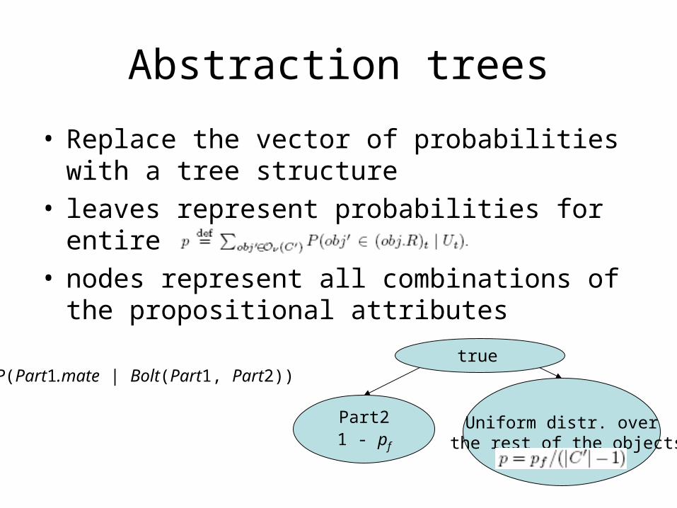
Abstraction trees
• Replace the vector of probabilities with a tree structure
• leaves represent probabilities for entire sets of objects
• nodes represent all combinations of the propositional attributes
Part21 - pf
Uniform distr. over the rest of the objects
trueP(Part1.mate | Bolt(Part1, Part2))

PLATE
weightshapecolor
PLATE
weightshapecolor
PLATE
weightshapecolor
Experiments
PLATE
weightshapecolor
PLATE
weightshapecolor
BRACKETweightshapecolor
welded tobolt
PLATE
weightshapecolor
PLATE
weightshapecolor
PLATE
weightshapecolor
BOLTweightsizetype
welded tobolt
PLATEweightshapecolor
welded tobolt
PLATE
weightshapecolor
PLATE
weightshapecolor
PLATE
weightshapecolor
ACTION
action
Dom(ACTION.action) ={paint, drill, polish,Change prop. Attr.,Change rel. Attr.}
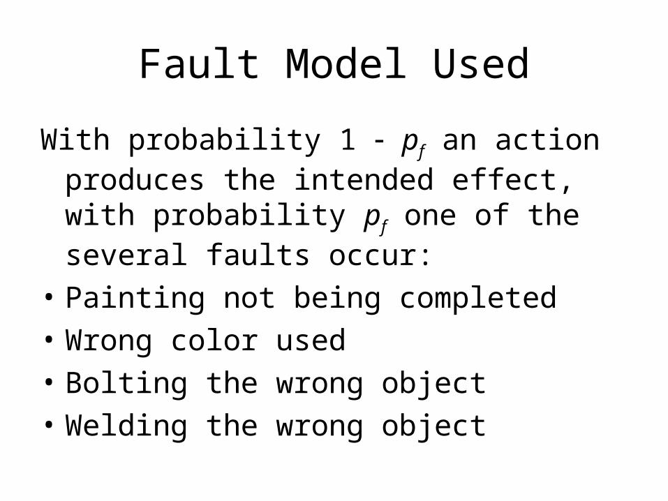
Fault Model Used
With probability 1 pf an action produces the intended effect, with probability pf one of the several faults occur:
• Painting not being completed
• Wrong color used
• Bolting the wrong object
• Welding the wrong object

Observation Model Used
With probability 1 po the truth value of the attribute is observed, with probability po an incorrect value is observed

Measure of the Accuracy
• K-L divergence between distributions
• Computing is infeasible – approximation is needed

Approximation of K-L Divergence
• We are interested only in measuring the differences in performance of different approximation methods -> first term is eliminated
• Take S samples from the true distribution (S = 10,000 in the experiments)


Experimental Results
• Abstraction trees reduced RBPF’s time and memory by a factor of 30 to 70
• On average six times longer and 11 times the memory of PF, per particle.
• However, note that we ran PF with 40 times more particles than RBPF.
• Thus, RBPF is using less time and memory than PF, and performing far better in accuracy.

Conclusions and future work
• Relaxing the assumptions made
• Further scaling up inference
• Studying the properties of the abstraction trees
• Handling continuous variables
• Learning DPRMs
• Applying them to the real world problems