DYNAMIC MODELLING OF CATALYTIC SO2 CONVERTER IN … Thesis... · THESIS DEFENCE COMMITTEE/COMITÉ DE SOUTENANCE DE THÈSE ... scholarly purposes may be granted by the professor or

DYNAMIC MODELLING OF CATALYTIC SO2 CONVERTER IN A SULFURIC ACID PLANT

OF AN INDUSTRIAL SMELTER

by

Jianjun He

Thesis submitted in partial fulfillment of the requirements for the degree of

Doctor of Philosophy (PhD) in Natural Resources Engineering

Faculty of Graduate Studies Laurentian University

Sudbury, Ontario, Canada

© Jianjun He, 2018

ii

THESIS DEFENCE COMMITTEE/COMITÉ DE SOUTENANCE DE THÈSE Laurentian Université/Université Laurentienne

Faculty of Graduate Studies/Faculté des études supérieures Title of Thesis Titre de la thèse DYNAMIC MODELLING OF CATALYTIC SO₂ CONVERTER IN A SULFURIC

ACID PLANT OF AN INDUSTRIAL SMELTER Name of Candidate Nom du candidat He, Jianjun Degree Diplôme Doctor of Philosophy Department/Program Date of Defence Département/Programme Natural Resoureces Engineering Date de la soutenance April 16, 2018

APPROVED/APPROUVÉ Thesis Examiners/Examinateurs de thèse: Dr. Helen Shang (Co-Supervisor/Co-directrice de thèse) Dr. Junfeng Zhang (Co-Supervisor/Co-directeur de thèse) Dr. Ramesh Subramanian (Committee member/Membre du comité) Dr. JA Scott (Committee member/Membre du comité) Approved for the Faculty of Graduate Studies Approuvé pour la Faculté des études supérieures Dr. David Lesbarrères Monsieur David Lesbarrères Dr. Ali Elkamel Dean, Faculty of Graduate Studies (External Examiner/Examinateur externe) Doyen, Faculté des études supérieures Dr. Guangdong Yang (Internal Examiner/Examinateur interne)

ACCESSIBILITY CLAUSE AND PERMISSION TO USE I, Jianjun He, hereby grant to Laurentian University and/or its agents the non-exclusive license to archive and make accessible my thesis, dissertation, or project report in whole or in part in all forms of media, now or for the duration of my copyright ownership. I retain all other ownership rights to the copyright of the thesis, dissertation or project report. I also reserve the right to use in future works (such as articles or books) all or part of this thesis, dissertation, or project report. I further agree that permission for copying of this thesis in any manner, in whole or in part, for scholarly purposes may be granted by the professor or professors who supervised my thesis work or, in their absence, by the Head of the Department in which my thesis work was done. It is understood that any copying or publication or use of this thesis or parts thereof for financial gain shall not be allowed without my written permission. It is also understood that this copy is being made available in this form by the authority of the copyright owner solely for the purpose of private study and research and may not be copied or reproduced except as permitted by the copyright laws without written authority from the copyright owner.

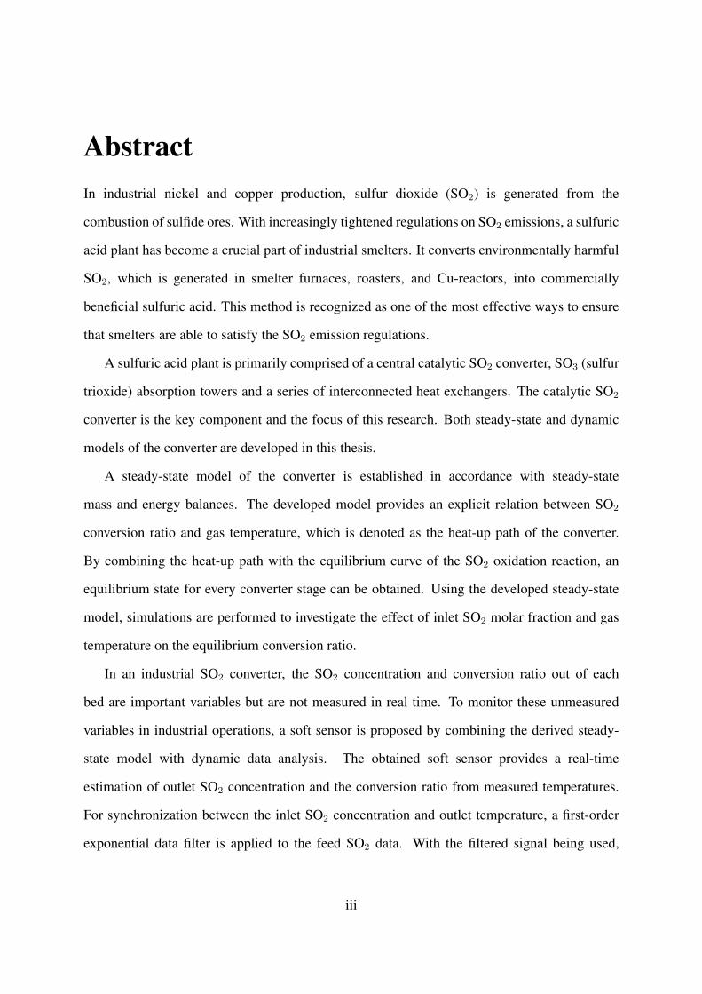
AbstractIn industrial nickel and copper production, sulfur dioxide (SO2) is generated from the

combustion of sulfide ores. With increasingly tightened regulations on SO2 emissions, a sulfuric

acid plant has become a crucial part of industrial smelters. It converts environmentally harmful

SO2, which is generated in smelter furnaces, roasters, and Cu-reactors, into commercially

beneficial sulfuric acid. This method is recognized as one of the most effective ways to ensure

that smelters are able to satisfy the SO2 emission regulations.

A sulfuric acid plant is primarily comprised of a central catalytic SO2 converter, SO3 (sulfur

trioxide) absorption towers and a series of interconnected heat exchangers. The catalytic SO2

converter is the key component and the focus of this research. Both steady-state and dynamic

models of the converter are developed in this thesis.

A steady-state model of the converter is established in accordance with steady-state

mass and energy balances. The developed model provides an explicit relation between SO2

conversion ratio and gas temperature, which is denoted as the heat-up path of the converter.

By combining the heat-up path with the equilibrium curve of the SO2 oxidation reaction, an

equilibrium state for every converter stage can be obtained. Using the developed steady-state

model, simulations are performed to investigate the effect of inlet SO2 molar fraction and gas

temperature on the equilibrium conversion ratio.

In an industrial SO2 converter, the SO2 concentration and conversion ratio out of each

bed are important variables but are not measured in real time. To monitor these unmeasured

variables in industrial operations, a soft sensor is proposed by combining the derived steady-

state model with dynamic data analysis. The obtained soft sensor provides a real-time

estimation of outlet SO2 concentration and the conversion ratio from measured temperatures.

For synchronization between the inlet SO2 concentration and outlet temperature, a first-order

exponential data filter is applied to the feed SO2 data. With the filtered signal being used,

iii

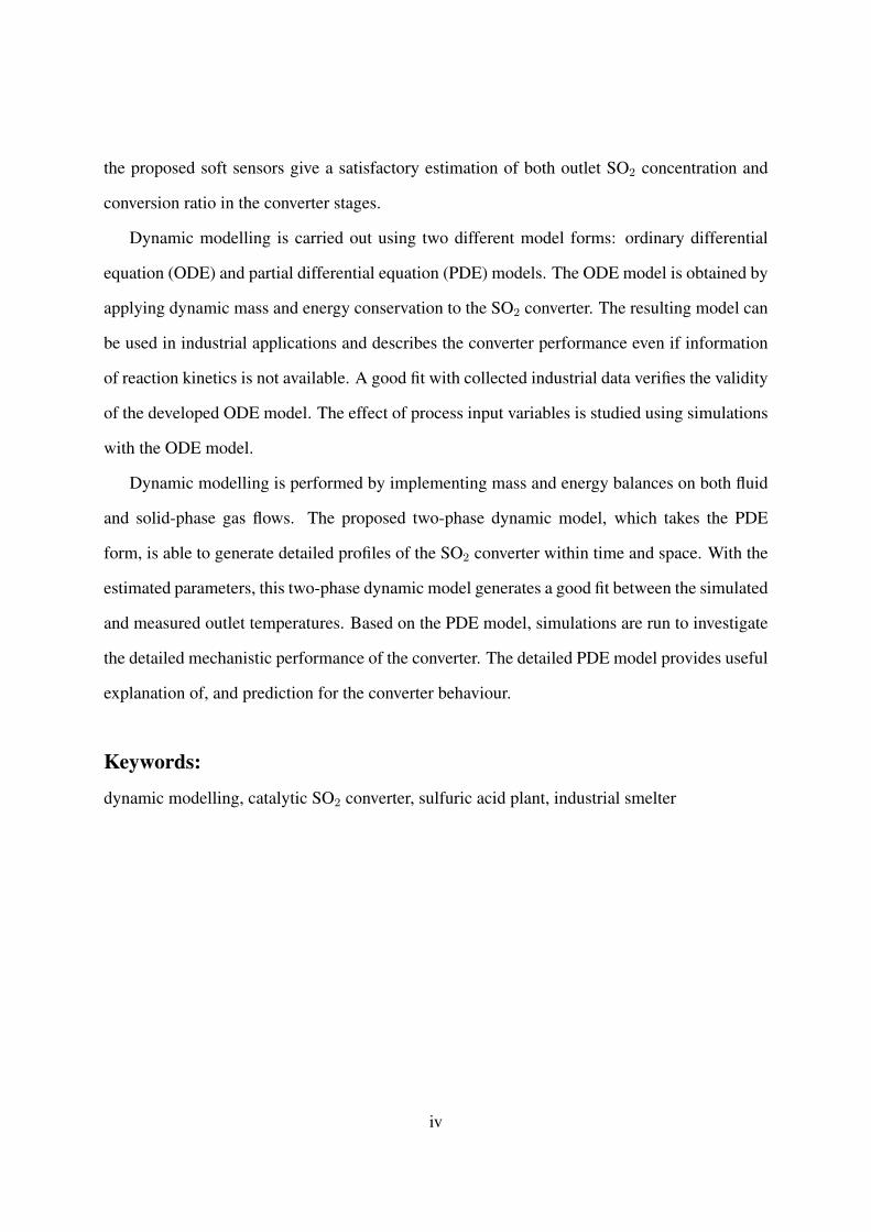
the proposed soft sensors give a satisfactory estimation of both outlet SO2 concentration and

conversion ratio in the converter stages.

Dynamic modelling is carried out using two different model forms: ordinary differential

equation (ODE) and partial differential equation (PDE) models. The ODE model is obtained by

applying dynamic mass and energy conservation to the SO2 converter. The resulting model can

be used in industrial applications and describes the converter performance even if information

of reaction kinetics is not available. A good fit with collected industrial data verifies the validity

of the developed ODE model. The effect of process input variables is studied using simulations

with the ODE model.

Dynamic modelling is performed by implementing mass and energy balances on both fluid

and solid-phase gas flows. The proposed two-phase dynamic model, which takes the PDE

form, is able to generate detailed profiles of the SO2 converter within time and space. With the

estimated parameters, this two-phase dynamic model generates a good fit between the simulated

and measured outlet temperatures. Based on the PDE model, simulations are run to investigate

the detailed mechanistic performance of the converter. The detailed PDE model provides useful

explanation of, and prediction for the converter behaviour.

Keywords:

dynamic modelling, catalytic SO2 converter, sulfuric acid plant, industrial smelter

iv

AcknowledgmentsI would like to express my sincere gratitude to my supervisor Dr. Helen Shang, who provided

me with the opportunity to start my Ph.D researching, guided me patiently throughout my

graduate studies, inspired me with her wisdom and professional expertise, and supported

me psychologically and financially. It was a pleasure for me to work and study under her

supervision.

I would like to acknowledge the patient guidance of Dr. Junfeng Zhang, who provided me

with professional suggestions and helped me solve various problems in the Ph.D research.

Also, I would like to thank my advisory committee: Dr. John A. Scott, Dr. Ramesh

Subramanian, Dr. Guangdong Yang and Dr. Ali Elkamel for their valuable time in helping

me with my Ph.D work and giving me insightful opinions to improve my thesis.

The financial support from Natural Sciences and Engineering Research Council of Canada

(NSERC), Vale Canada Inc. and Laurentian University is gratefully acknowledged. The

industrial data and process information from Vales Copper Cliff Smelter are especially

appreciated. The support and guidance by Chris Doyle, Dan Legrand and Paul Kenny from

Vale is particularly appreciated.

v

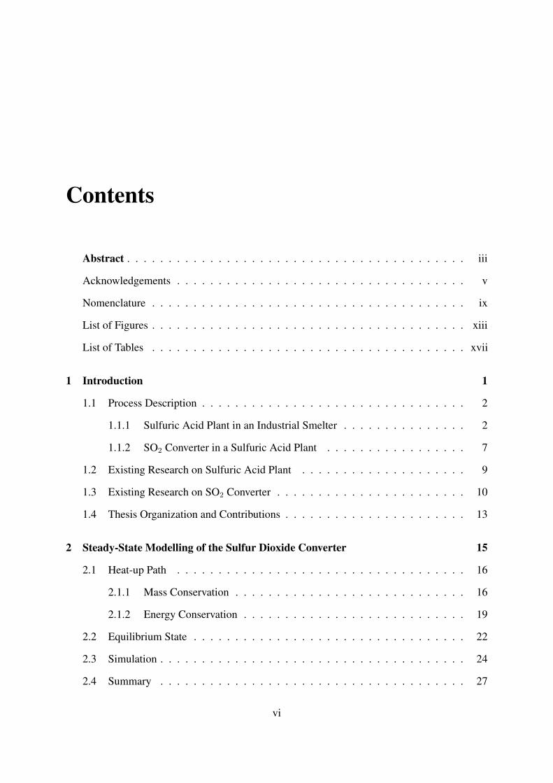
Contents

Abstract . . . . . . . . . . . . . . . . . . . . . . . . . . . . . . . . . . . . . . . . . iii

Acknowledgements . . . . . . . . . . . . . . . . . . . . . . . . . . . . . . . . . . . v

Nomenclature . . . . . . . . . . . . . . . . . . . . . . . . . . . . . . . . . . . . . . ix

List of Figures . . . . . . . . . . . . . . . . . . . . . . . . . . . . . . . . . . . . . . xiii

List of Tables . . . . . . . . . . . . . . . . . . . . . . . . . . . . . . . . . . . . . . xvii

1 Introduction 1

1.1 Process Description . . . . . . . . . . . . . . . . . . . . . . . . . . . . . . . . 2

1.1.1 Sulfuric Acid Plant in an Industrial Smelter . . . . . . . . . . . . . . . 2

1.1.2 SO2 Converter in a Sulfuric Acid Plant . . . . . . . . . . . . . . . . . 7

1.2 Existing Research on Sulfuric Acid Plant . . . . . . . . . . . . . . . . . . . . 9

1.3 Existing Research on SO2 Converter . . . . . . . . . . . . . . . . . . . . . . . 10

1.4 Thesis Organization and Contributions . . . . . . . . . . . . . . . . . . . . . . 13

2 Steady-State Modelling of the Sulfur Dioxide Converter 15

2.1 Heat-up Path . . . . . . . . . . . . . . . . . . . . . . . . . . . . . . . . . . . 16

2.1.1 Mass Conservation . . . . . . . . . . . . . . . . . . . . . . . . . . . . 16

2.1.2 Energy Conservation . . . . . . . . . . . . . . . . . . . . . . . . . . . 19

2.2 Equilibrium State . . . . . . . . . . . . . . . . . . . . . . . . . . . . . . . . . 22

2.3 Simulation . . . . . . . . . . . . . . . . . . . . . . . . . . . . . . . . . . . . . 24

2.4 Summary . . . . . . . . . . . . . . . . . . . . . . . . . . . . . . . . . . . . . 27

vi

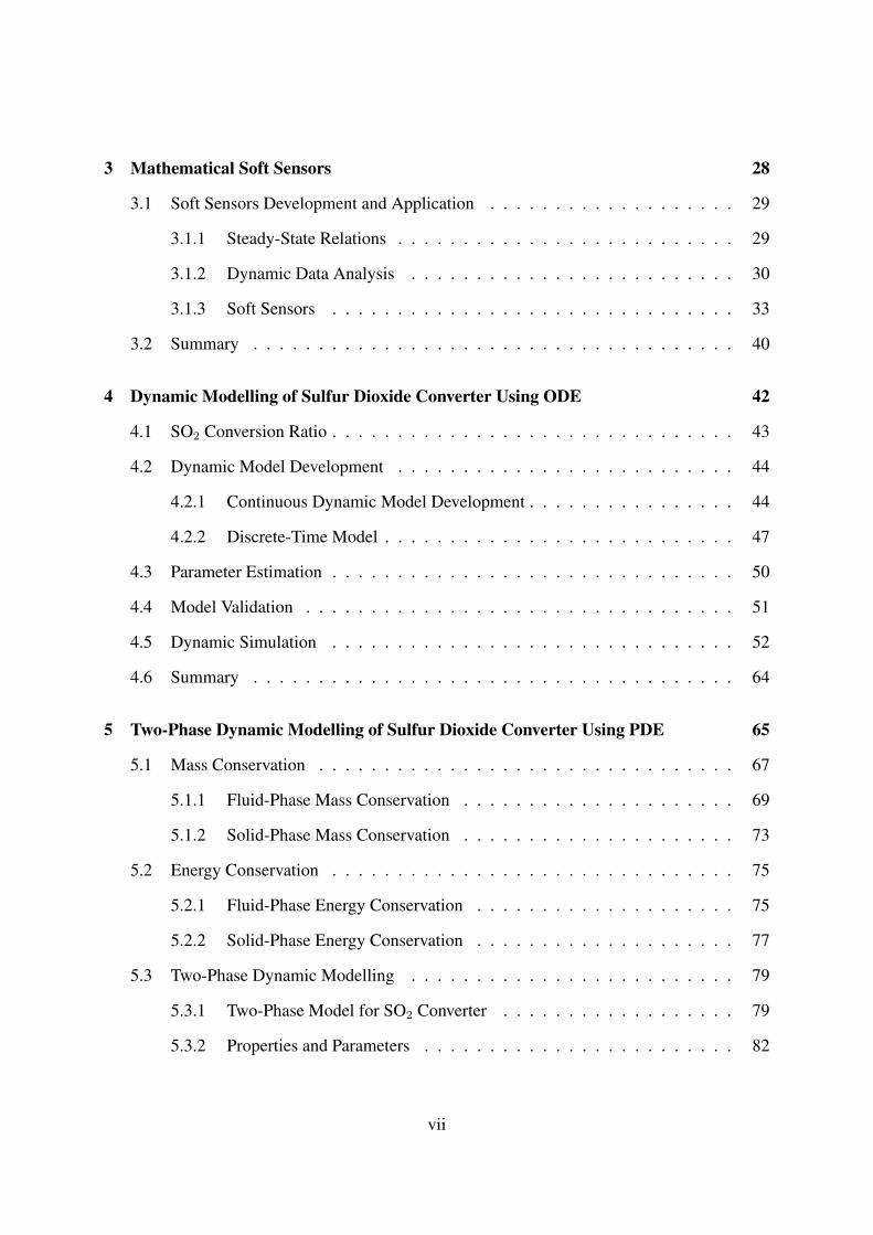
3 Mathematical Soft Sensors 28

3.1 Soft Sensors Development and Application . . . . . . . . . . . . . . . . . . . 29

3.1.1 Steady-State Relations . . . . . . . . . . . . . . . . . . . . . . . . . . 29

3.1.2 Dynamic Data Analysis . . . . . . . . . . . . . . . . . . . . . . . . . 30

3.1.3 Soft Sensors . . . . . . . . . . . . . . . . . . . . . . . . . . . . . . . 33

3.2 Summary . . . . . . . . . . . . . . . . . . . . . . . . . . . . . . . . . . . . . 40

4 Dynamic Modelling of Sulfur Dioxide Converter Using ODE 42

4.1 SO2 Conversion Ratio . . . . . . . . . . . . . . . . . . . . . . . . . . . . . . . 43

4.2 Dynamic Model Development . . . . . . . . . . . . . . . . . . . . . . . . . . 44

4.2.1 Continuous Dynamic Model Development . . . . . . . . . . . . . . . . 44

4.2.2 Discrete-Time Model . . . . . . . . . . . . . . . . . . . . . . . . . . . 47

4.3 Parameter Estimation . . . . . . . . . . . . . . . . . . . . . . . . . . . . . . . 50

4.4 Model Validation . . . . . . . . . . . . . . . . . . . . . . . . . . . . . . . . . 51

4.5 Dynamic Simulation . . . . . . . . . . . . . . . . . . . . . . . . . . . . . . . 52

4.6 Summary . . . . . . . . . . . . . . . . . . . . . . . . . . . . . . . . . . . . . 64

5 Two-Phase Dynamic Modelling of Sulfur Dioxide Converter Using PDE 65

5.1 Mass Conservation . . . . . . . . . . . . . . . . . . . . . . . . . . . . . . . . 67

5.1.1 Fluid-Phase Mass Conservation . . . . . . . . . . . . . . . . . . . . . 69

5.1.2 Solid-Phase Mass Conservation . . . . . . . . . . . . . . . . . . . . . 73

5.2 Energy Conservation . . . . . . . . . . . . . . . . . . . . . . . . . . . . . . . 75

5.2.1 Fluid-Phase Energy Conservation . . . . . . . . . . . . . . . . . . . . 75

5.2.2 Solid-Phase Energy Conservation . . . . . . . . . . . . . . . . . . . . 77

5.3 Two-Phase Dynamic Modelling . . . . . . . . . . . . . . . . . . . . . . . . . 79

5.3.1 Two-Phase Model for SO2 Converter . . . . . . . . . . . . . . . . . . 79

5.3.2 Properties and Parameters . . . . . . . . . . . . . . . . . . . . . . . . 82

vii

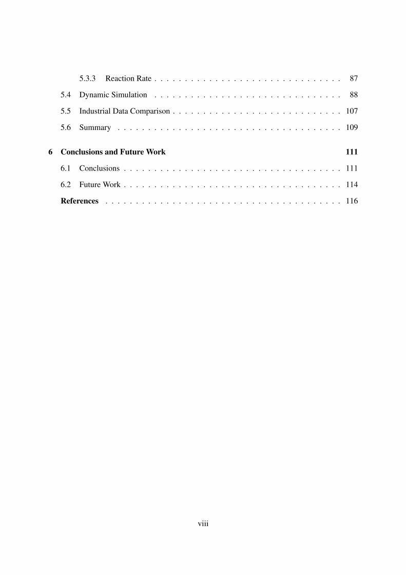
5.3.3 Reaction Rate . . . . . . . . . . . . . . . . . . . . . . . . . . . . . . . 87

5.4 Dynamic Simulation . . . . . . . . . . . . . . . . . . . . . . . . . . . . . . . 88

5.5 Industrial Data Comparison . . . . . . . . . . . . . . . . . . . . . . . . . . . . 107

5.6 Summary . . . . . . . . . . . . . . . . . . . . . . . . . . . . . . . . . . . . . 109

6 Conclusions and Future Work 111

6.1 Conclusions . . . . . . . . . . . . . . . . . . . . . . . . . . . . . . . . . . . . 111

6.2 Future Work . . . . . . . . . . . . . . . . . . . . . . . . . . . . . . . . . . . . 114

References . . . . . . . . . . . . . . . . . . . . . . . . . . . . . . . . . . . . . . . 116

viii

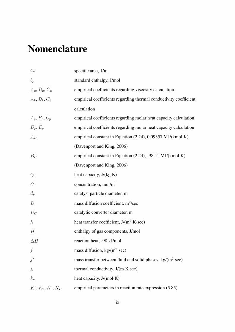
Nomenclature

ap specific area, 1/m

bp standard enthalpy, J/mol

Aµ, Bµ, Cµ empirical coefficients regarding viscosity calculation

Ak, Bk, Ck empirical coefficients regarding thermal conductivity coefficient

calculation

Ap, Bp, Cp empirical coefficients regarding molar heat capacity calculation

Dp, Ep empirical coefficients regarding molar heat capacity calculation

AE empirical constant in Equation (2.24), 0.09357 MJ/(kmol·K)

(Davenport and King, 2006)

BE empirical constant in Equation (2.24), -98.41 MJ/(kmol·K)

(Davenport and King, 2006)

cp heat capacity, J/(kg·K)

C concentration, mol/m3

dp catalyst particle diameter, m

D mass diffusion coefficient, m2/sec

DC catalytic converter diameter, m

h heat transfer coefficient, J/(m2·K·sec)

H enthalpy of gas components, J/mol

∆H reaction heat, -98 kJ/mol

j mass diffusion, kg/(m2·sec)

j∗ mass transfer between fluid and solid phases, kg/(m2·sec)

k thermal conductivity, J/(m·K·sec)

kp heat capacity, J/(mol·K)

K1, K2, K3, KE empirical parameters in reaction rate expression (5.85)

ix

nt total molar quantity of gas in the converter stage, mol

M molecular weight, g/mol

N molar flowrate, mol/sec

P pressure, Pa

Pr Prandtl number

q heat flux, J/(m2·sec)

Q volume flowrate, m3/sec

Q heat flux rate, J/sec

r consumption rate of SO2, mol/min

rSO2 production rate of SO2, mol/(kg-cat·sec)

rh energy release rate of chemical reation, J/(kg-cat·sec)

rs chemical production rate, mol/(kg-cat·sec)

R ideal gas constant, 0.008314 kJ/(mol·K)

Rs chemical production rate, kg/(kg-cat·sec)

Re Reynolds number

S area, m2

Sc Schmidt number

t time, sec

T temperature, K

Tcp specific temperature defined as T /1000, 10−3K

u Darcy velocity, m/sec

v average velocity, m/sec

V volume, m3

Vsp specific volume, m3

Vm molar volume at normal boiling point, cm3/mol

x gas flow direction

x

X molar fraction of gas compoenents

y, z radial directions of the catalyst bed

Greek symbols

α first-order exponential filter parameter

β mass transfer coefficient, m/sec

ε porosity

κ Darcy permeability, m2

λ parameter related with actural and equilibrium SO2 conversion ratios

µ viscosity, Pa·sec

Φ SO2 conversion ratio

π ratio of a circle’s circumference to its diameter, 3.1416

ρ density, kg/m3

Superscript

E equilibrium

in inlet

Subscript

cat catalyst

cs cross-section

cv control volume

f fluid phase

g gas

i represents gas components, SO2, O2, SO3 or nonreactive remainders

k stages of the converter

xi

min minimum

max maximum

p catalyst particle

re nonreactive remainders in the gas mixture

s solid phase

t total

xii

List of Figures

1.1 Flowsheet of sulfuric acid making from smelting and converting off-gas

(Schlesinger et al., 2011) . . . . . . . . . . . . . . . . . . . . . . . . . . . . . 4

1.2 Schematic diagram of major operating units in a sulfuric acid plant . . . . . . . 5

1.3 Schematic diagram of a SO3 absorption tower (Davenport and King, 2006) . . . 6

2.1 Schematic diagram of a catalytic SO2 converter stage . . . . . . . . . . . . . . 15

2.2 First-bed heat-up path under a given feed condition . . . . . . . . . . . . . . . 20

2.3 First-bed heat-up path under different inlet SO2 concentrations . . . . . . . . . 22

2.4 Equilibrium curve combining the first-bed heat-up path . . . . . . . . . . . . . 23

2.5 Conversion-temperature diagram for three catalyst beds under different inlet

temperatures . . . . . . . . . . . . . . . . . . . . . . . . . . . . . . . . . . . . 24

2.6 Conversion-temperature diagram for three catalyst beds under different inlet

SO2 concentrations . . . . . . . . . . . . . . . . . . . . . . . . . . . . . . . . 25

2.7 Conversion-temperature diagram for the first bed under different gas pressures . 26

3.1 Structure of the XSO2 and Φ soft sensors for a SO2 converter stage. . . . . . . . 30

3.2 Dynamic evolvement of outlet temperature in response to a feed concentration

decrease. . . . . . . . . . . . . . . . . . . . . . . . . . . . . . . . . . . . . . . 31

3.3 Dynamic evolvement of outlet temperature in response to feed concentration

changes. . . . . . . . . . . . . . . . . . . . . . . . . . . . . . . . . . . . . . . 32

3.4 Correlation coefficient between X in(t) and T (t+ ∆t) with different time shifts. 33

xiii

3.5 Correlation coefficient between the filtered X in(t) and T (t+ ∆t) with different

time shifts. . . . . . . . . . . . . . . . . . . . . . . . . . . . . . . . . . . . . . 35

3.6 Comparison of dynamics of the filtered feed molar fraction and measured outlet

temperature when there is a decrease in feed molar fraction. . . . . . . . . . . . 36

3.7 Comparison of dynamics of the filtered feed molar fraction and measured outlet

temperature when there are changes in feed molar fraction. . . . . . . . . . . . 36

3.8 Feed temperature and filtered feed temperature corresponding to operation in

Figure 3.2. . . . . . . . . . . . . . . . . . . . . . . . . . . . . . . . . . . . . . 37

3.9 Estimated conversion ratio and molar fraction of SO2 for a step decrease in SO2

feed molar fraction as in Figure 3.2. . . . . . . . . . . . . . . . . . . . . . . . 38

3.10 Estimated conversion ratio and molar fraction of SO2 for step changes in SO2

feed molar fraction as in Figure 3.3. . . . . . . . . . . . . . . . . . . . . . . . 38

3.11 Comparison of SO2 conversion ratio estimates for a step decrease in SO2 feed

molar fraction as in Figure 3.2. . . . . . . . . . . . . . . . . . . . . . . . . . . 40

4.1 Two periods of one-day measured and predicted outlet temperature comparison

of the four-bed SO2 converter . . . . . . . . . . . . . . . . . . . . . . . . . . . 53

4.2 Comparison of the first-bed measured and predicted outlet temperature in

response to inlet SO2 changes . . . . . . . . . . . . . . . . . . . . . . . . . . . 54

4.3 Outlet SO2 concentration and overall SO2 conversion ratio estimation after

filtering the first-bed feed SO2 concentration . . . . . . . . . . . . . . . . . . . 55

4.4 Dynamic simulation on outlet temperatures of four catalyst beds in response to

a step change on first-bed inlet SO2 concentration . . . . . . . . . . . . . . . . 57

4.5 Dynamic simulation on first-bed outlet temperature in response to a step change

on the first-bed inlet SO2 concentration under different flowrates . . . . . . . . 58

4.6 Outlet SO2 concentrations, overall SO2 conversion ratios and outlet temperature

under different feed SO2 concentrations . . . . . . . . . . . . . . . . . . . . . 60

xiv


under different feed temperatures . . . . . . . . . . . . . . . . . . . . . . . . . 61


under different inlet O2 to SO2 concentration ratios . . . . . . . . . . . . . . . 62

5.1 Schematic diagram of the catalyst particle packing inside a SO2 converter stage 65

5.2 A converter stage and an infinitesimal control volume . . . . . . . . . . . . . . 67

5.3 Simulated spatial variation profiles of fluid- and solid-phase outlet temperatures

and SO2 concentrations . . . . . . . . . . . . . . . . . . . . . . . . . . . . . . 90

5.4 Simulated spatial profiles of steady-state reaction rate and SO2 conversion ratio 91

5.5 Comparison of simulated and equilibrium outlet SO2 concentration and

conversion ratio . . . . . . . . . . . . . . . . . . . . . . . . . . . . . . . . . . 91

5.6 Spatial profiles of fluid- and solid-phase temperature and SO2 concentration

after inlet SO2 cut-off . . . . . . . . . . . . . . . . . . . . . . . . . . . . . . . 93

5.7 Detailed spatial profiles of individual energy terms on solid-phase temperature

dynamics after inlet SO2 cut-off . . . . . . . . . . . . . . . . . . . . . . . . . 94

5.8 Detailed spatial profiles of individual energy terms on fluid-phase temperature

dynamics after inlet SO2 cut-off . . . . . . . . . . . . . . . . . . . . . . . . . 95

5.9 Spatial profiles of fluid- and solid-phase temperature and SO2 concentration

after inlet SO2 restoration . . . . . . . . . . . . . . . . . . . . . . . . . . . . . 96

5.10 Detailed spatial profiles of individual energy terms on solid-phase temperature

dynamics after inlet SO2 restoration . . . . . . . . . . . . . . . . . . . . . . . 97

5.11 Detailed spatial profiles of individual energy terms on fluid-phase temperature

dynamics after inlet SO2 restoration . . . . . . . . . . . . . . . . . . . . . . . 97

5.12 Simulated outlet temperature profiles during inlet SO2 cut-off and restoring cases 98

5.13 Heat loss flux rate of the catalyst bed after inlet SO2 cut-off and heat gain flux

rate of the catalyst bed after inlet SO2 restoration . . . . . . . . . . . . . . . . 99

xv

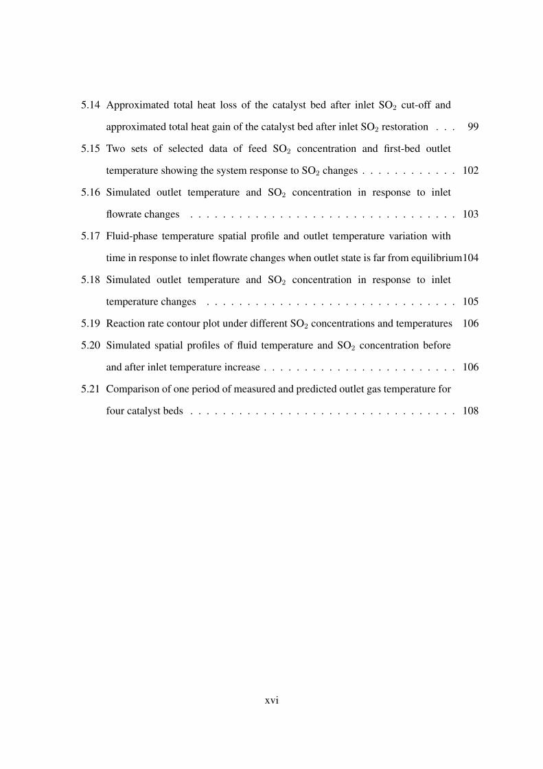
5.14 Approximated total heat loss of the catalyst bed after inlet SO2 cut-off and

approximated total heat gain of the catalyst bed after inlet SO2 restoration . . . 99

5.15 Two sets of selected data of feed SO2 concentration and first-bed outlet

temperature showing the system response to SO2 changes . . . . . . . . . . . . 102

5.16 Simulated outlet temperature and SO2 concentration in response to inlet

flowrate changes . . . . . . . . . . . . . . . . . . . . . . . . . . . . . . . . . 103

5.17 Fluid-phase temperature spatial profile and outlet temperature variation with

time in response to inlet flowrate changes when outlet state is far from equilibrium104

5.18 Simulated outlet temperature and SO2 concentration in response to inlet

temperature changes . . . . . . . . . . . . . . . . . . . . . . . . . . . . . . . 105

5.19 Reaction rate contour plot under different SO2 concentrations and temperatures 106

5.20 Simulated spatial profiles of fluid temperature and SO2 concentration before

and after inlet temperature increase . . . . . . . . . . . . . . . . . . . . . . . . 106

5.21 Comparison of one period of measured and predicted outlet gas temperature for

four catalyst beds . . . . . . . . . . . . . . . . . . . . . . . . . . . . . . . . . 108

xvi

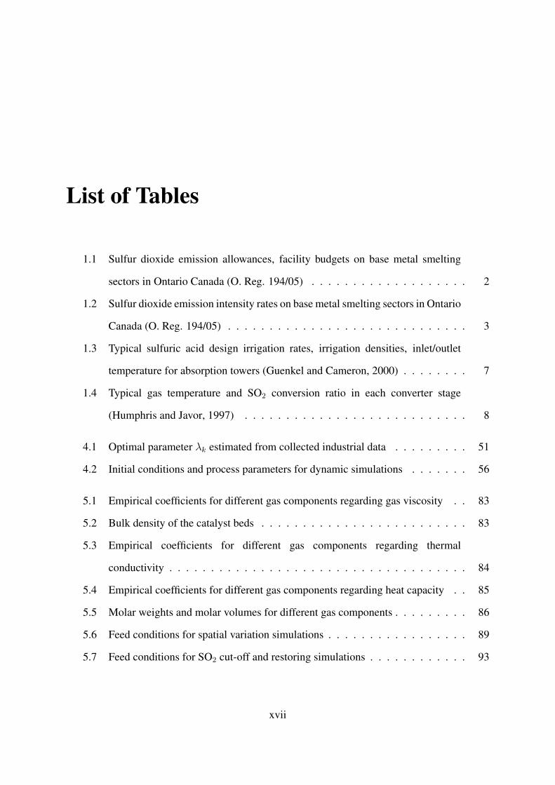
List of Tables

1.1 Sulfur dioxide emission allowances, facility budgets on base metal smelting

sectors in Ontario Canada (O. Reg. 194/05) . . . . . . . . . . . . . . . . . . . 2

1.2 Sulfur dioxide emission intensity rates on base metal smelting sectors in Ontario

Canada (O. Reg. 194/05) . . . . . . . . . . . . . . . . . . . . . . . . . . . . . 3

1.3 Typical sulfuric acid design irrigation rates, irrigation densities, inlet/outlet

temperature for absorption towers (Guenkel and Cameron, 2000) . . . . . . . . 7

1.4 Typical gas temperature and SO2 conversion ratio in each converter stage

(Humphris and Javor, 1997) . . . . . . . . . . . . . . . . . . . . . . . . . . . 8

4.1 Optimal parameter λk estimated from collected industrial data . . . . . . . . . 51

4.2 Initial conditions and process parameters for dynamic simulations . . . . . . . 56

5.1 Empirical coefficients for different gas components regarding gas viscosity . . 83

5.2 Bulk density of the catalyst beds . . . . . . . . . . . . . . . . . . . . . . . . . 83

5.3 Empirical coefficients for different gas components regarding thermal

conductivity . . . . . . . . . . . . . . . . . . . . . . . . . . . . . . . . . . . . 84

5.4 Empirical coefficients for different gas components regarding heat capacity . . 85

5.5 Molar weights and molar volumes for different gas components . . . . . . . . . 86

5.6 Feed conditions for spatial variation simulations . . . . . . . . . . . . . . . . . 89

5.7 Feed conditions for SO2 cut-off and restoring simulations . . . . . . . . . . . . 93

xvii

Chapter 1

Introduction

Apart from the sulfur-laden fossil fuel combustion, smelting of sulfide ores to extract the

designated metal has become a major source of sulfur dioxide (SO2) emission into the

atmosphere (Ciccone and Storbeck, 1997). SO2 is recognized worldwide as a significant air

pollutant and the major cause of acid rain, resulting in harmful impacts on human respiratory

systems and the environment (Kampa and Castanas, 2008). SO2 generated from industrial

smelters was historically directly discharged into the atmosphere without proper treatments, and

led to a wide range of severe environmental issues (Chan et al., 1984a,b). In order to reduce SO2

emissions, significant efforts were subsequently made through different abatement programs at

many smelters (Hunter Jr. et al., 1975; Donovan et al., 1978; Sudbury and Crawford, 1989;

Gunn et al., 1995; Byrdziak et al., 1996; Lobanov et al., 2008; Ma et al., 2012).

Sulfuric acid plants are markedly important in the modern process industry due to wide

applications of sulfuric acid products (e.g., fertilizers, metallic ore leaching and petroleum (Kiss

et al., 2010)). As they are capable of capturing sulfur dioxide in off-gas, sulfuric acid plants

have also become an essential part of many smelters. A typical sulfuric acid plant is primarily

composed of a central catalytic SO2 converter, SO3 (sulfur trioxide) absorption towers, and a

series of interconnected heat exchangers. The central catalytic converter, where SO2 is oxidized

by oxygen (O2) to SO3, is usually built with multistage catalyst beds. It determines the amount

1

of SO2 captured from the off-gas and is the key unit in a sulfuric acid plant.

1.1 Process Description

1.1.1 Sulfuric Acid Plant in an Industrial Smelter

Sulfuric acid is a bedrock of the modern chemical industry and is widely used in many industrial

sectors. The raw material of sulfuric acid is sulfur dioxide (SO2) gas, which mostly originates

from elemental sulfur burning, metal sulfide ore smelting, and/or spent acid (Davenport and

King, 2006; Ashar and Golwalkar, 2013). Unlike SO2 gas from sulfur burners, where SO2

concentration is controllable and easily maintained, SO2 in metallurgical off-gas is often dusty

and can vary in concentration. This makes the SO2 conversion and acid production more

challenging. According to an air pollutant emission report from Environment and Climate

Change Canada, 46% of Canada’s sulfur oxide (SOx) pollutant in 2015 came from the oil and

mineral industries (ECCC, 2017). In Ontario Canada, smelters resulted in over 60% of sulfur

dioxide emissions in 2012 (MECC-SO2). In order to control and reduce the SO2 emission,

increasingly stringent environmental regulations on discharge levels have been issued in many

districts or countries.

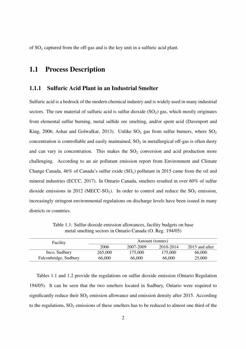
Table 1.1: Sulfur dioxide emission allowances, facility budgets on basemetal smelting sectors in Ontario Canada (O. Reg. 194/05)

Facility Amount (tonnes)2006 2007-2009 2010-2014 2015 and after

Inco, Sudbury 265,000 175,000 175,000 66,000Falconbridge, Sudbury 66,000 66,000 66,000 25,000

Tables 1.1 and 1.2 provide the regulations on sulfur dioxide emission (Ontario Regulation

194/05). It can be seen that the two smelters located in Sudbury, Ontario were required to

significantly reduce their SO2 emission allowance and emission density after 2015. According

to the regulations, SO2 emissions of these smelters has to be reduced to almost one third of the

2

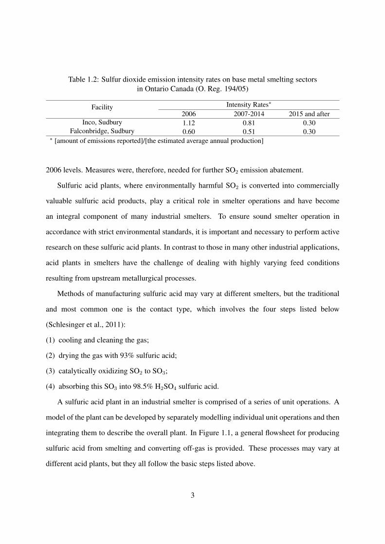
Table 1.2: Sulfur dioxide emission intensity rates on base metal smelting sectorsin Ontario Canada (O. Reg. 194/05)

Facility Intensity Rates∗

2006 2007-2014 2015 and afterInco, Sudbury 1.12 0.81 0.30

Falconbridge, Sudbury 0.60 0.51 0.30∗ [amount of emissions reported]/[the estimated average annual production]

2006 levels. Measures were, therefore, needed for further SO2 emission abatement.

Sulfuric acid plants, where environmentally harmful SO2 is converted into commercially

valuable sulfuric acid products, play a critical role in smelter operations and have become

an integral component of many industrial smelters. To ensure sound smelter operation in

accordance with strict environmental standards, it is important and necessary to perform active

research on these sulfuric acid plants. In contrast to those in many other industrial applications,

acid plants in smelters have the challenge of dealing with highly varying feed conditions

resulting from upstream metallurgical processes.

Methods of manufacturing sulfuric acid may vary at different smelters, but the traditional

and most common one is the contact type, which involves the four steps listed below

(Schlesinger et al., 2011):

(1) cooling and cleaning the gas;

(2) drying the gas with 93% sulfuric acid;

(3) catalytically oxidizing SO2 to SO3;

(4) absorbing this SO3 into 98.5% H2SO4 sulfuric acid.

A sulfuric acid plant in an industrial smelter is comprised of a series of unit operations. A

model of the plant can be developed by separately modelling individual unit operations and then

integrating them to describe the overall plant. In Figure 1.1, a general flowsheet for producing

sulfuric acid from smelting and converting off-gas is provided. These processes may vary at

different acid plants, but they all follow the basic steps listed above.

3

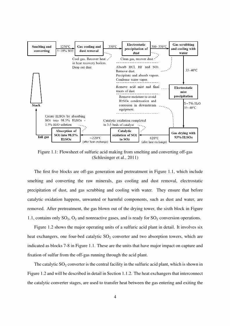
Figure 1.1: Flowsheet of sulfuric acid making from smelting and converting off-gas(Schlesinger et al., 2011)

The first five blocks are off-gas generation and pretreatment in Figure 1.1, which include

smelting and converting the raw minerals, gas cooling and dust removal, electrostatic

precipitation of dust, and gas scrubbing and cooling with water. They ensure that before

catalytic oxidation happens, unwanted or harmful components, such as dust and water, are

removed. After pretreatment, the gas blown out of the drying tower, the sixth block in Figure

1.1, contains only SO2, O2 and nonreactive gases, and is ready for SO2 conversion operations.

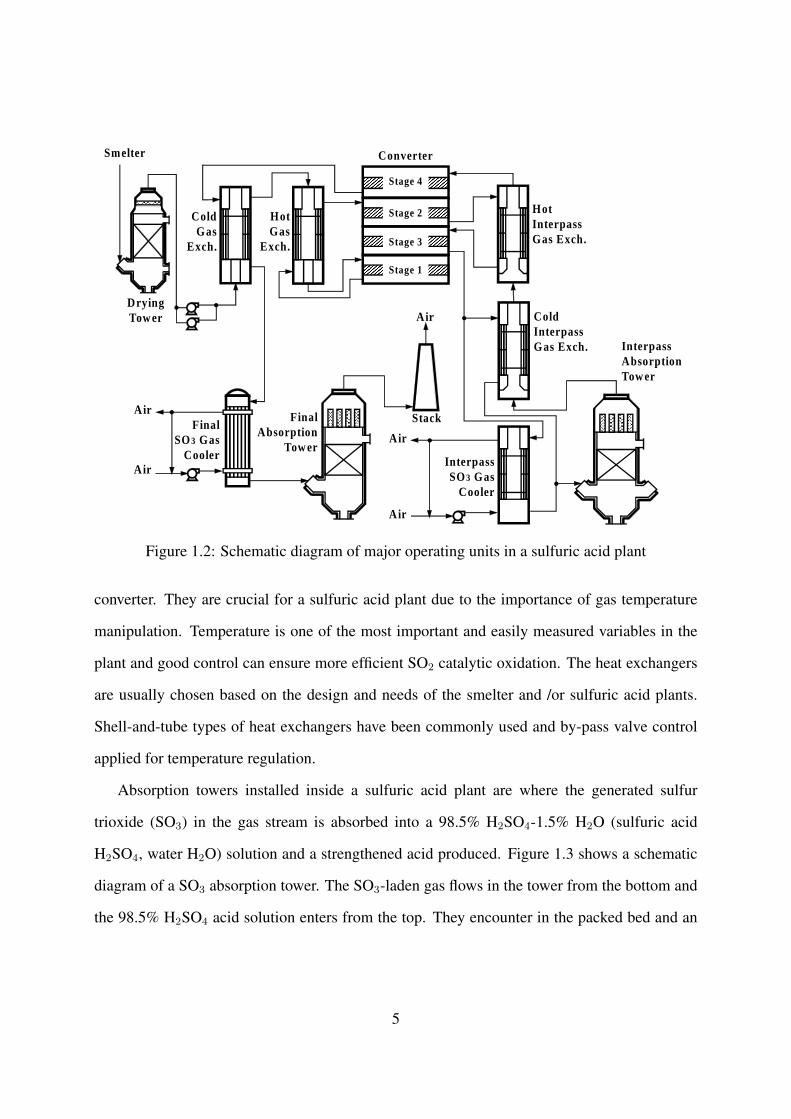
Figure 1.2 shows the major operating units of a sulfuric acid plant in detail. It involves six

heat exchangers, one four-bed catalytic SO2 converter and two absorption towers, which are

indicated as blocks 7-8 in Figure 1.1. These are the units that have major impact on capture and

fixation of sulfur from the off-gas running through the acid plant.

The catalytic SO2 converter is the central facility in the sulfuric acid plant, which is shown in

Figure 1.2 and will be described in detail in Section 1.1.2. The heat exchangers that interconnect

the catalytic converter stages, are used to transfer heat between the gas entering and exiting the

4

��

��

��

��Stage 1

Stage 3

Stage 2

Stage 4

��

��

��

��

��

��

��

��

��

Converter Smelter

Drying Tow er

Cold Gas

Exch.

Hot Gas

Exch.

Hot Interpass Gas Exch.

Cold Interpass Gas Exch.

Interpass SO 3 Gas

Cooler

Final SO 3 Gas

Cooler

Interpass Absorption Tow er

Final Absorption

Tow er

Stack

Air

Air

Air

Air

Air

Figure 1.2: Schematic diagram of major operating units in a sulfuric acid plant

converter. They are crucial for a sulfuric acid plant due to the importance of gas temperature

manipulation. Temperature is one of the most important and easily measured variables in the

plant and good control can ensure more efficient SO2 catalytic oxidation. The heat exchangers

are usually chosen based on the design and needs of the smelter and /or sulfuric acid plants.

Shell-and-tube types of heat exchangers have been commonly used and by-pass valve control

applied for temperature regulation.

Absorption towers installed inside a sulfuric acid plant are where the generated sulfur

trioxide (SO3) in the gas stream is absorbed into a 98.5% H2SO4-1.5% H2O (sulfuric acid

H2SO4, water H2O) solution and a strengthened acid produced. Figure 1.3 shows a schematic

diagram of a SO3 absorption tower. The SO3-laden gas flows in the tower from the bottom and

the 98.5% H2SO4 acid solution enters from the top. They encounter in the packed bed and an

5

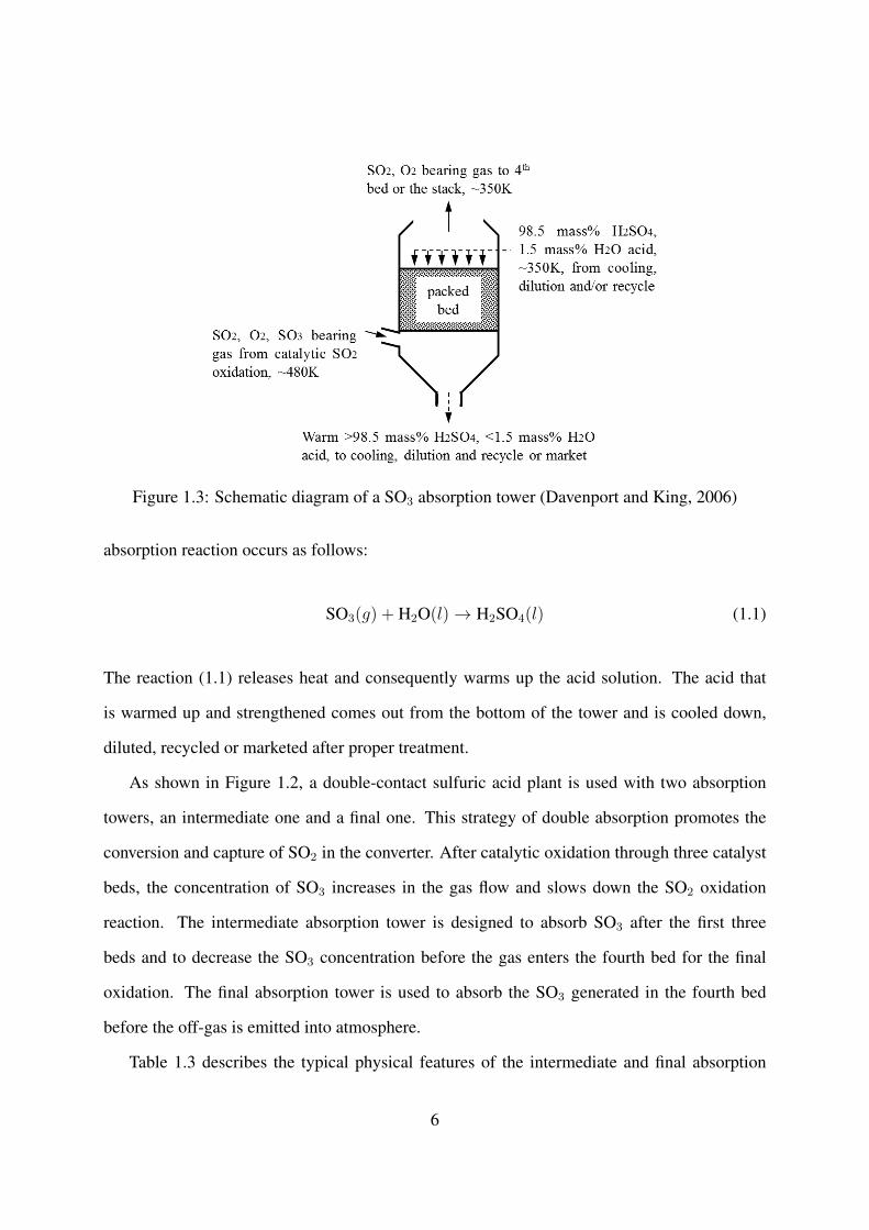
Figure 1.3: Schematic diagram of a SO3 absorption tower (Davenport and King, 2006)

absorption reaction occurs as follows:

SO3(g) + H2O(l)→ H2SO4(l) (1.1)

The reaction (1.1) releases heat and consequently warms up the acid solution. The acid that

is warmed up and strengthened comes out from the bottom of the tower and is cooled down,

diluted, recycled or marketed after proper treatment.

As shown in Figure 1.2, a double-contact sulfuric acid plant is used with two absorption

towers, an intermediate one and a final one. This strategy of double absorption promotes the

conversion and capture of SO2 in the converter. After catalytic oxidation through three catalyst

beds, the concentration of SO3 increases in the gas flow and slows down the SO2 oxidation

reaction. The intermediate absorption tower is designed to absorb SO3 after the first three

beds and to decrease the SO3 concentration before the gas enters the fourth bed for the final

oxidation. The final absorption tower is used to absorb the SO3 generated in the fourth bed

before the off-gas is emitted into atmosphere.

Table 1.3 describes the typical physical features of the intermediate and final absorption

6

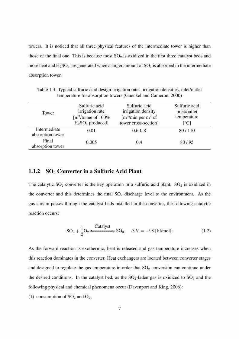
towers. It is noticed that all three physical features of the intermediate tower is higher than

those of the final one. This is because most SO2 is oxidized in the first three catalyst beds and

more heat and H2SO4 are generated when a larger amount of SO3 is absorbed in the intermediate

absorption tower.

Table 1.3: Typical sulfuric acid design irrigation rates, irrigation densities, inlet/outlettemperature for absorption towers (Guenkel and Cameron, 2000)

TowerSulfuric acid Sulfuric acid Sulfuric acidirrigation rate irrigation density inlet/outlet

[m3/tonne of 100% [m3/min per m2 of temperatureH2SO4 produced] tower cross-section] [◦C]

Intermediate 0.01 0.6-0.8 80 / 110absorption tower

Final 0.005 0.4 80 / 95absorption tower

1.1.2 SO2 Converter in a Sulfuric Acid Plant

The catalytic SO2 converter is the key operation in a sulfuric acid plant. SO2 is oxidized in

the converter and this determines the final SO2 discharge level to the environment. As the

gas stream passes through the catalyst beds installed in the converter, the following catalytic

reaction occurs:

SO2 +1

2O2

CatalystEGGGGGGGGGGGGGGGGGGGGGGGGC SO3, ∆H = −98 [kJ/mol]. (1.2)

As the forward reaction is exothermic, heat is released and gas temperature increases when

this reaction dominates in the converter. Heat exchangers are located between converter stages

and designed to regulate the gas temperature in order that SO2 conversion can continue under

the desired conditions. In the catalyst bed, as the SO2-laden gas is oxidized to SO3 and the

following physical and chemical phenomena occur (Davenport and King, 2006):

(1) consumption of SO2 and O2;

7

(2) production of SO3;

(3) heating the descending gas;

(4) heat exchange between gas and catalyst bed.

Reaction (1.2) occurring in the converter requires a suitable catalyst. Without this catalyst,

the exothermic reaction barely occurs. The typical catalyst used in (1.2) is V2O5-K2SO4 based,

and contains 5-10% V2O5, 10-20% K2SO4, 1-5% Na2SO4, and 55-70% SiO2 (Schlesinger et al.,

2011). SiO2 is an inactive material, but serves as a support for the other components. However,

the catalyst is not always active and effective at all ranges of temperature. When the temperature

of the catalyst drops below its ignition temperature, which is around 360◦C for the V2O5-K2SO4

based catalyst, the reaction proceeds very slowly or even stops. Whereas an overly heated

catalyst bed, typically over 650◦C, could lead to deactivation of catalyst or even unrecoverable

damage. The temperature in the converter must, therefore, be maintained between ignition and

degradation temperatures, in order to achieve effective SO2 conversion.

Sometimes, the catalyst component K2SO4 is replaced by cesium sulfate, Cs2SO4, because

a Cs2SO4-based catalyst can lower the activation temperature as well as provide a higher

reaction rate. However, the cesium-based catalyst costs more than the K2SO4-based one. Some

plants, therefore, only apply a Cs-based catalyst to the first catalyst bed where the majority of

conversion happens (Schlesinger et al., 2011) or mix with K2SO4.

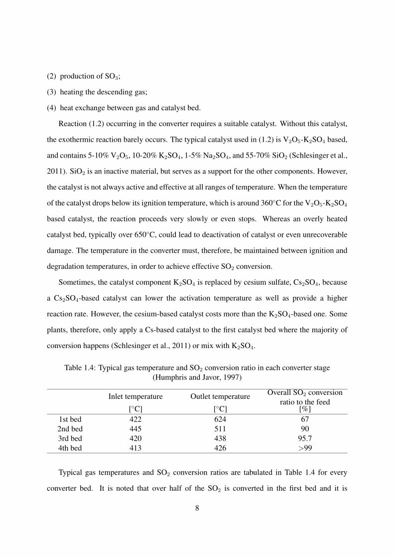
Table 1.4: Typical gas temperature and SO2 conversion ratio in each converter stage(Humphris and Javor, 1997)

Inlet temperature Outlet temperature Overall SO2 conversionratio to the feed

[◦C] [◦C] [%]1st bed 422 624 672nd bed 445 511 903rd bed 420 438 95.74th bed 413 426 >99

Typical gas temperatures and SO2 conversion ratios are tabulated in Table 1.4 for every

converter bed. It is noted that over half of the SO2 is converted in the first bed and it is

8

thus crucial to maintain an optimal operation in this bed to achieve the best overall SO2

conversion. As shown in Table 1.4, conversion efficiency decreases in the subsequent stages

due to continuous consumption of SO2. After the off-gas stream passes through all the catalyst

beds, over 99% of SO2 will be captured by the acid plant.

1.2 Existing Research on Sulfuric Acid Plant

Sulfuric acid plants are essential for the modern process industry due to sulfuric acid’s wide

range of industrial applications, which include fertilizers, metallic ore leaching, and petroleum

(Kiss et al., 2010; Schlesinger et al., 2011). Following the development of vanadium catalysts,

the contact process started taking over the traditional chamber process in sulfuric acid plants in

the early 1900’s. Not only did it sharply increase productivity, it also encouraged improvement

of equipment and materials in each area of the process (Friedman, 1999). With awareness of

the environmental impacts of sulfur dioxide on our communities, as one of the most effective

ways to capture and fix sulfur dioxide from ore processing off-gases (Friedman and Friedman,

2006), sulfuric acid plants have also established a vital environmental protection role.

Among research on sulfuric acid plants, the start-up of the plants gets a lot of attention.

Start-up study is important because due to a low temperature of the gas and the catalyst, little

or no SO2 will be converted into sulfuric acid before the desired temperature is achieved. As a

consequence, unconverted SO2 could be discharged into the atmosphere. Furthermore, a large

amount of heat is needed to heat up the plant during the start-up process.

Mann et al. investigated the start-up of a sulfuric acid plant and found that with a proper

manipulation of sulfur burning-rate, the problem of over-emitted SO2 could be solved with a

fast start-up (Mann et al., 1980). Afterwards, they came up with a new idea to obtain fast

and clean start-up, which required suitable flowrate programming in accordance with initial

bed temperatures (Mann, 1986). In addition, software system was developed to address start-

up problems, with the advantage of applying to all kinds of plant flowsheets (Gosiewski and

9

Klaudel, 1985).

Along with improvements in sulfuric acid plant technologies, research on the design,

modification, optimization and operational problems have been carried out. Based on

calculating the conversion and pressure drop, a SO2 optimization program was developed

by Donovan et al. that the operators could use of for better plant design and operation

(Donovan et al., 1978). The frequent fluctuation of SO2 concentration in the feed gas, as a

consequence of multiple feed sources to acid plants, is a challenging problem. An analysis of

the dynamic resistance of the concentration drop in the plant was conducted with two selected

characteristic flowsheets of metallurgical SO2 oxidation plants, and helped provide an insight

into the influence of concentration changes (Gosiewski, 1996).

Dynamic models were provided by Shang et al. for an industrial smelter off-gas system

based on mass, momentum, and energy conservation laws (Shang et al., 2008). These served

as an alternative method to solve feed gas problem of a sulfuric acid plant by dealing with

the source concentration of SO2. Raw material selection and/or upstream technology were

mentioned in (Liang and Liang, 2013) and an acid plant studied in terms of equipment,

integrity of instrumentation control and the proficiency of personnel operation. Model-based

optimization of sulfur recovery with a network design connecting the reactor, furnace and waste

heat boiler of the sulfur recovery units together was found useful for integrated process-energy

optimization (Manenti et al., 2014).

A good review of unit operations in the plant, including gas cleaning and the contact

sections, equipment design, materials and handling stream variables and impurities, can be

found in (Friedman and Friedman, 2006).

1.3 Existing Research on SO2 Converter

SO2 converters are the central unit operation in a sulfuric acid plant on account of their SO2

capture and conversion function. Due to their importance, research on this facility is crucial

10

and much of it has been focussed on modelling the SO2 reactors. Mann and his colleagues

proposed a dynamic simulation model using ordinary differential equations to describe the

unsteady behaviour of the fixed-bed reactors, and it was used as a base to set up fast start-

up (Mann et al., 1980). Mann also mentioned that the advantage of using ordinary differential

equations over partial differential ones lied in the fact that each bed of the reactor comprised

of catalyst pellets and could be easily represented by a set of back mixed stages (Mann, 1986).

Using a spreadsheet, Davenport and King presented an introduction to sulfuric acid manufacture

with the calculation of steady-state operations (Davenport and King, 2006).

Modelling of the reactors has been beneficial to the operation, optimization, and control

of sulfuric acid plants. A one-dimensional heterogeneous model was employed to simulate an

adiabatic periodic flow reversal reactor (Snyder and Subramaniam, 1993). It was focussed

on simulating the effect of operating conditions and feed gas temperature variations, and

found that reaction extinction can be presented by changes in operating conditions. Another

one-dimensional two-phase unsteady-state model studied mass conservation of SO2 and the

heat for each phase (Hong et al., 1997). To solve this model, which was built with partial

differential equations, Hong et al. applied the Crank-Nicolson predictor-corrector method and

the numerical results indicated that oxidation of low concentration sulfur dioxide is possible.

To handle a low concentration of sulfur dioxide for oxidation, Xiao et al. suggested a converter

configuration and a dual position control strategy from modelling, a laboratory reactor and a

pilot scale converter (Xiao et al., 1999). The adiabatic assumption is usually made in modelling,

even though the adiabatic requirement of the reactors is hard to achieve. Modelling of the

reactors and simulation could be used for compensation of the adiabatic requirement and to

obtain better model-based performance (Xiao and Yuan, 1996).

By introducing a correction factor into a global rate equation, Wu and his colleagues

came up with a heterogeneous transient model to study catalytic oxidation of sulfur dioxide

and successfully predicted transient concentration and temperature profiles (Wu et al., 1996).

11

Through considering the dynamic properties of the vanadium catalyst, mathematical modelling

of sulfur dioxide oxidation was carried out using the nonstationary state of the catalyst surface

(Vernikovskaya et al., 1999). It was concluded that it can be applied to a conventional double

contact/double absorption sulfuric acid plant.

For good temperature control, an experimental and modelling study was made of a

packed-bed reactor with the assumption of pseudo-homogeneous perfect plug flow (Nouri and

Ouederni, 2013). It was found that conversion decreases with the amount of SO2 and increases

with temperature before an optimum is reached. A good reaction rate model can help improve

the accuracy and performance of reactor models. Ravindra et al. presented a reaction rate

model based on complete wetting of the catalyst particles in a trickle-bed reactor (Ravindra

et al., 1997), and this model could predict reaction rate trends during sulfur dioxide oxidation.

An important breakthrough was made with a more detailed dynamic model developed

for an acid plant using partial differential equations, and the model was simulated using

the software gPROM (Kiss et al., 2010). The model used partial differential equations and

developed dynamic models for three-phase slurry and trickle-bed reactors. A method using

finite difference approximation for the spatial derivatives was investigated, and the simulations

showed that the dynamic approach generates important information on reaction dynamics

(Warna and Salmi, 1996).

Even though extensive researches have been done on SO2 converter, some problems still

require further investigation. Some important variables, for example, SO2 conversion ratio,

are important for SO2 converter modelling, but are rarely measured in the plant. Research on

the soft sensor developments for these unmeasured variables are necessary. In addition, the

available dynamic models of SO2 converter are complicated and inconvenient for industrial

applications, or have mismatch problems with the industrial system. Furthermore, mechanism

study inside the SO2 converter is still limited. These problems will all be covered and

investigated in my PhD research.

12

1.4 Thesis Organization and Contributions

This dissertation contains six chapters. Chapter 1 presents the process description and literature

review over sulfuric acid plants and SO2 converters. The contributions of the research are

provided in Chapter 2 to Chapter 5, followed by the conclusions and suggested future work in

Chapter 6.

Chapter 2 establishes the steady-state model of catalytic SO2 converter based on steady-state

mass and energy balances. The obtained model describes the relation between gas temperature

and SO2 conversion ratio under given feed conditions, and provides the base for the dynamic

modelling, simplification, and optimization found in the following chapters. Incorporated with

the equilibrium curve of reaction (1.2), the potential maximum conversion of the converter can

be calculated by using the proposed steady-state relation, which is also called as the heat-up

path.

In the derivation of the steady-state model in Chapter 2, expressions of steady-state outlet

SO2 concentration and SO2 conversion ratio are obtained. Chapter 3 incorporates the industrial

dynamic data analysis with these expressions to derive mathematical soft sensors for outlet

SO2 concentration and the SO2 conversion ratio. A first-order exponential filter is applied

to the SO2 feed concentration so that synchronization between the filtered concentration and

outlet temperature is achieved. The proposed soft sensors are able to estimate the unmeasured

variables for the catalytic SO2 converter using available industrial measurements.

In Chapter 4, by applying mass and energy conservation, dynamic modelling of the SO2

converter is carried out in the form of ordinary differential equations (ODE). This dynamic

modelling uses the SO2 conversion ratio as the key variable, and gives an acceptable prediction

of converter output responses. A good match is achieved between model predicted values

and industrial measurements. Based on this ODE model, the effect of input variables on the

performance of the converter is investigated.

13

In Chapter 5, mechanistic modelling for the SO2 converter is studied by considering the gas

in both fluid and solid phases. Detailed two-phase dynamic modelling in the form of partial

differential equations (PDE) is performed based on mass and energy balances of both the fluid

and solid phases. Using the developed dynamic model, spatial profiles of the temperature and

concentration are given by simulations, and the effects of the process variables investigated. By

analyzing the dynamics of two phases through detailed simulations, the different dynamics of

outlet temperature in response to feed SO2 cut-off and restoration can be effectively explained.

As the outlet temperature prediction from the two-phase model has a satisfactory fit with

industrial data, the model provides, therefore, a useful tool in studying the mechanisms of

an industrial SO2 converter and in predicting process performance under different operating

conditions.

14

Chapter 2

Steady-State Modelling of the Sulfur

Dioxide Converter

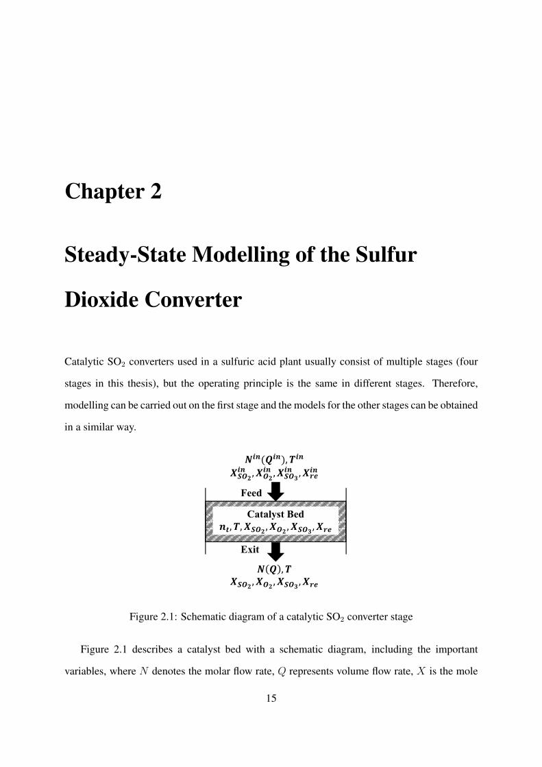
Catalytic SO2 converters used in a sulfuric acid plant usually consist of multiple stages (four

stages in this thesis), but the operating principle is the same in different stages. Therefore,

modelling can be carried out on the first stage and the models for the other stages can be obtained

in a similar way.

Catalyst Bed

Feed

Exit

Figure 2.1: Schematic diagram of a catalytic SO2 converter stage

Figure 2.1 describes a catalyst bed with a schematic diagram, including the important

variables, where N denotes the molar flow rate, Q represents volume flow rate, X is the mole

15

fraction (concentration) with subscripts indicating individual components in the gas and the

superscript “in” standing for the feed condition, T represents the temperature, and nt is the

molar quantity of the gas in the converter stage.

Steady-state model is built based on the steady-state mass and energy balances of the off-gas

within the converter stage. It is formulated to explore the relationship among the key variables

and to provide a foundation for dynamic modelling and soft sensors. For steady-state modelling,

the following assumptions are made:

(1) the converter is assumed to be adiabatic;

(2) temperature difference between gas and catalyst bed is negligible.

2.1 Heat-up Path

2.1.1 Mass Conservation

Considering a catalyst stage illustrated in Figure 2.1, the offgas contains both reactive

components (SO2, O2 and SO3) and nonreactive components (expressed by subscript “re” for

remainders). According to the reaction (1.2), the conversion involves sulfur (S) and oxygen (O)

elements. Applying the mole balances to these two elements during the reaction, yields:

X inSO2

N in +X inSO3

N in = XSO2N +XSO3N (2.1)

2X inSO2

N in + 2X inO2N in + 3X in

SO3N in = 2XSO2N + 2XO2N + 3XSO3N (2.2)

As the nonreactive components are not involved in the reaction, the mole balance on these

components can simply be written as:

X inreN

in = XreN (2.3)

16

The molar fraction of the remainder gas in the offgas can be expressed as:

X inre = 1−X in

SO2−X in

O2−X in

SO3(2.4)

Xre = 1−XSO2 −XO2 −XSO3 (2.5)

In a SO2 converter, it is important to examine the ratio of oxidized SO2 at each stage under

different conditions. This conversion ratio Φ reflects the performance of the converter and can

be defined as the ratio of SO2 that is oxidized to SO3:

Φ =X inSO2

N in −XSO2N

X inSO2

N in. (2.6)

Based on (2.6), XSO2 can be written as a function of the conversion ratio and feed conditions:

XSO2 = (1− Φ)X inSO2

N in

N. (2.7)

The expressions for XO2 , XSO3 and Xre are obtained by substituting (2.7) to Equations (2.1 -

2.3):

XO2 =

(X inO2− 1

2ΦX in

SO2

)N in

N, (2.8)

XSO3 =(X inSO3

+ ΦX inSO2

) N in

N, (2.9)

Xre =(1−X in

SO2−X in

O2−X in

SO3

) N in

N, (2.10)

For the reaction (1.2), for each mole of SO2 being converted, there is one half mole reduction

in the total mole amount. The outlet mole flow rate N can therefore be written as:

N =

(1− 1

2ΦX in

SO2

)N in, (2.11)

17

and the ratio of N in to N is:N in

N=

1

1− 1

2ΦX in

SO2

. (2.12)

Substituting Equation (2.12) into Equations (2.7 - 2.10), the mole fractions of different

components are then derived:

XSO2 =(1− Φ)X in

SO2

1− 1

2ΦX in

SO2

, (2.13)

XO2 =X inO2− 1

2ΦX in

SO2

1− 1

2ΦX in

SO2

, (2.14)

XSO3 =X inSO3

+ ΦX inSO2

1− 1

2ΦX in

SO2

, (2.15)

Xre =1−X in

SO2−X in

O2−X in

SO3

1− 1

2ΦX in

SO2

. (2.16)

It is noted that under a specified feed condition, the mole fractions of all components vary with

the conversion ratio. Substituting (2.11) into (2.6), the conversion ratio Φ also takes the form as

a function of XSO2:

Φ =X inSO2−XSO2

X inSO2− 1

2XSO2X

inSO2

. (2.17)

The equation above can be used to exactly calculate the conversion ratio when SO2

concentration is measured.

18

2.1.2 Energy Conservation

If the converter is assumed to be adiabatic, the steady-state energy balance in the catalyst bed

illustrated in Figure 2.1 can thus be written as:

X inSO2

N inH inSO2

+X inO2N inH in

O2+X in

SO3N inH in

SO3+X in

reNinH in

re

= XSO2NHSO2 +XO2NHO2 +XSO3NHSO3 +XreNHre,

(2.18)

where H [J/mol] denotes the enthalpy of every mole gas component. Substituting Equations

(2.7 - 2.10) to (2.18), the energy equation becomes:

X inSO2

(H inSO2−HSO2) +X in

O2(H in

O2−HO2) +X in

SO3(H in

SO3−HSO3) +X in

re (Hinre −Hre)

=−(HSO2 +

1

2HO2 −HSO3

)ΦX in

SO2.

(2.19)

The enthalpies in the above equation are functions of temperature. While temperature changes

within a given range, the relation between enthalpy and temperature can be approximated to be

linear (Davenport and King, 2006),

H = kpT + bp, (2.20)

where kp is the heat capacity of the gas and bp is the standard enthalpy. The values of kp and bp

for the offgas components are given as (Davenport and King, 2006):

kp,SO2 = 0.05161 [kJ/(mol·K)], bp,SO2 = −314.3 [kJ/mol]

kp,O2 = 0.03333 [kJ/(mol·K)], bp,O2 = −10.79 [kJ/mol]

kp,SO3 = 0.07144 [kJ/(mol·K)], bp,SO3 = −420.6 [kJ/mol]

kp,N2 = 0.03110 [kJ/(mol·K)], bp,N2 = −9.797 [kJ/mol]

19

As the majority of nonreactive components is nitrogen gas, the heat capacity and the standard

enthalpy of the remainders are assumed to be equal to the ones of nitrogen gas. Substituting

Equation (2.20) to (2.19), the conversion ratio Φ is found related with the gas temperature in

the following expression:

Φ =(X in

SO2kp,SO2 +X in

O2kp,O2 +X in

SO3kp,SO3 +X in

rekp,N2)(T − T in)[(kp,SO2 +

1

2kp,O2 − kp,SO3

)T +

(bp,SO2 +

1

2bp,O2 − bp,SO3

)]X inSO2

(2.21)

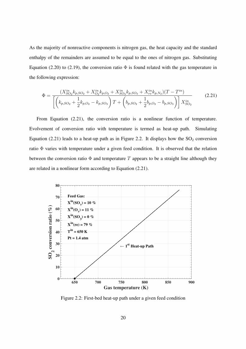
From Equation (2.21), the conversion ratio is a nonlinear function of temperature.

Evolvement of conversion ratio with temperature is termed as heat-up path. Simulating

Equation (2.21) leads to a heat-up path as in Figure 2.2. It displays how the SO2 conversion

ratio Φ varies with temperature under a given feed condition. It is observed that the relation

between the conversion ratio Φ and temperature T appears to be a straight line although they

are related in a nonlinear form according to Equation (2.21).

Gas temperature (K)

650 700 750 800 850 900

SO

2 c

on

ver

sio

n r

ati

o (

%)

0

10

20

30

40

50

60

70

80

Feed Gas:

Xin

(SO2) = 10 %

Xin

(O2) = 11 %

Xin

(SO3) = 0 %

Xin

(re) = 79 %

Tin

= 650 K

Pt = 1.4 atm

← 1st

Heat-up Path

Figure 2.2: First-bed heat-up path under a given feed condition

20

The approximate linearity can be obtained by approximating (2.21). Defining two molar

specific heat coefficients as:

kinp = X inSO2

kSO2 +X inO2kO2 +X in

SO3kSO3 +X in

rekN2 ,

kp = XSO2kSO2 +XO2kO2 +XSO3kSO3 +XrekN2 ,

under the normal operating condition, it holds that:

∣∣∣∣(kp,SO2 +1

2kp,O2 − kp,SO3

)T

∣∣∣∣ << ∣∣∣∣bp,SO2 +1

2bp,O2 − bp,SO3

∣∣∣∣and

bp,SO2 +1

2bp,O2 − bp,SO3 ≈ −∆H (2.22)

where−∆H indicates the standard reaction enthalpy in reaction (1.2). Equation (2.21) can then

be approximated as:

Φ ≈kinp

(−∆H)X inSO2

(T − T in) (2.23)

Relation between the conversion ratio and temperature is, therefore, approximately linear.

A similar linear expression to Equation (2.23) is mentioned in (Mann, 1986). Equation

(2.23) indicates that the slope of the heat-up path in Figure 2.2 changes with different feed

composition while the feed temperature determines the beginning intercept of the heat-up path.

kinp represents the molar heat capacity of the inlet feed gas. For the offgas generated under

regular operations, the value of kp barely varies. Therefore, the slope of heat-up path is mainly

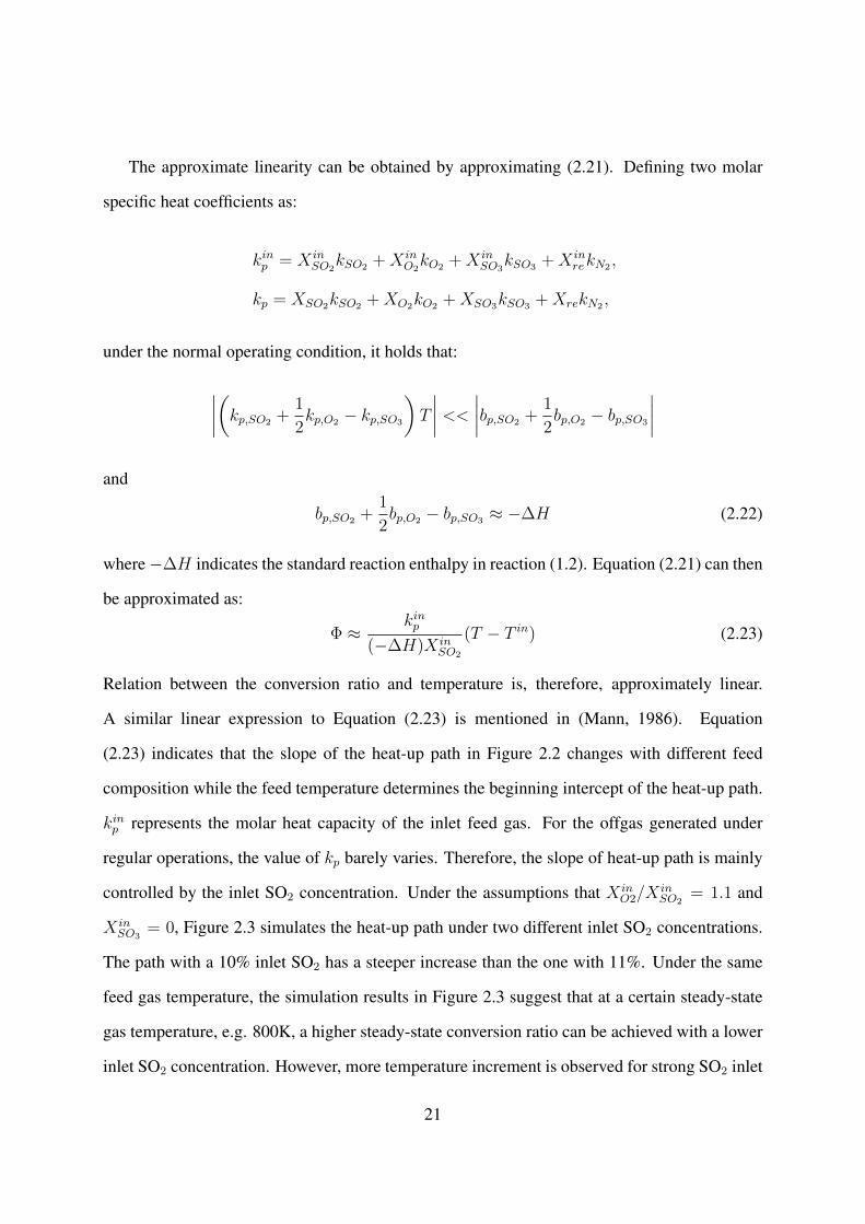
controlled by the inlet SO2 concentration. Under the assumptions that X inO2/X

inSO2

= 1.1 and

X inSO3

= 0, Figure 2.3 simulates the heat-up path under two different inlet SO2 concentrations.

The path with a 10% inlet SO2 has a steeper increase than the one with 11%. Under the same

feed gas temperature, the simulation results in Figure 2.3 suggest that at a certain steady-state

gas temperature, e.g. 800K, a higher steady-state conversion ratio can be achieved with a lower

inlet SO2 concentration. However, more temperature increment is observed for strong SO2 inlet

21

as per percentage conversion occurs due to more amount of SO2 is converted.

Gas temperature (K)

700 750 800 850 900

SO

2 c

on

ver

sio

n r

ati

o (

%)

0

10

20

30

40

50

60

70

Feed Gas:

Xin

(O2)/X

in(SO

2) = 1.1

Xin

(SO3) = 0 %

Tin

= 700 K

Pt = 1.4 atm

Xin

(SO2) = 10% →

Feed Gas:

Xin

(O2)/X

in(SO

2) = 1.1

Xin

(SO3) = 0 %

Tin

= 700 K

Pt = 1.4 atm

← Xin

(SO2) = 11%

Figure 2.3: First-bed heat-up path under different inlet SO2 concentrations

2.2 Equilibrium State

As the reaction (1.2) proceeds, the conversion ratio and temperature increase along the heat-up

path in Figure 2.2. With more SO2 is converted to SO3, the forward reaction rate decreases

and the reverse reaction rate increases. When the net reaction rate becomes zero, the reaction

reaches equilibrium. At equilibrium, the conversion ratio is related to temperature by the

following form (Davenport and King, 2006):

TE =−BE

AE +R · ln

[X inSO3

+X inSO2

ΦE

(1− ΦE)X inSO2

·(

1− 0.5X inSO2

ΦE

X inO2− 0.5X in

SO2ΦE

) 12

· P− 12

t

] . (2.24)

22

where Pt indicates the total pressure and R is the gas constant. AE and BE are empirical

constants and their values are given:

AE = 0.09357 [MJ/(kmol · K)],

BE = −98.41 [MJ/kmol],

R = 0.008314 [kJ/(mol · K)].

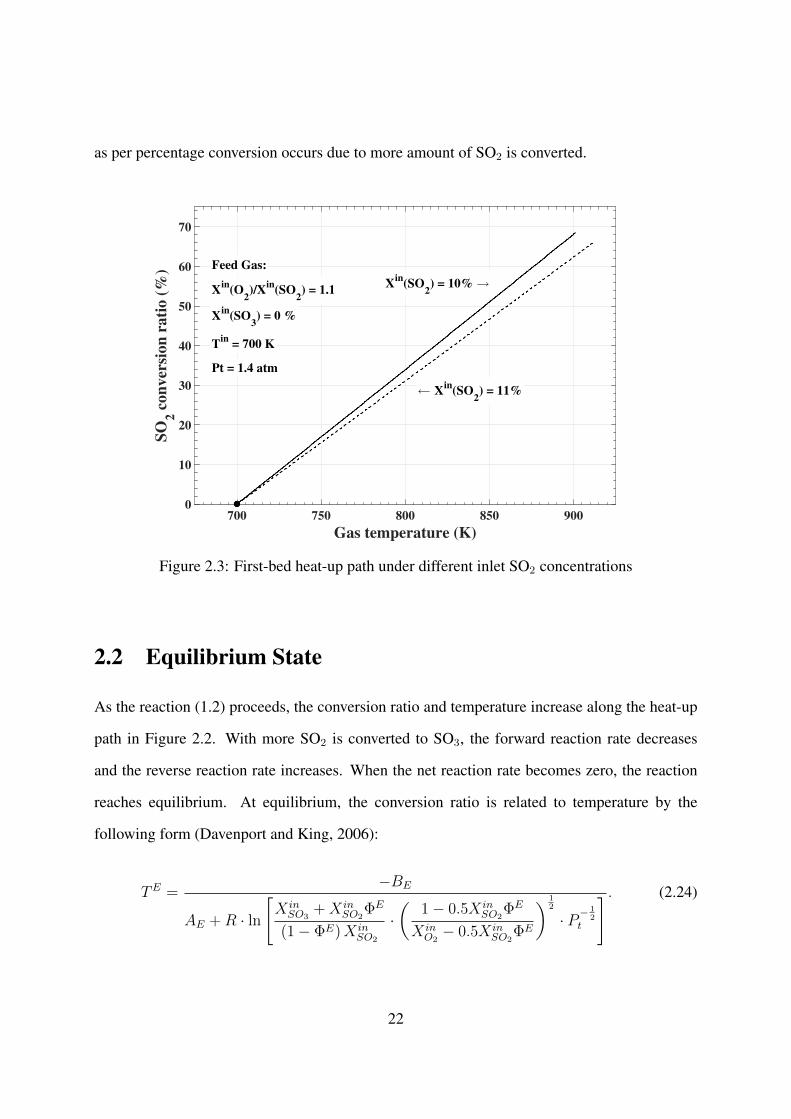
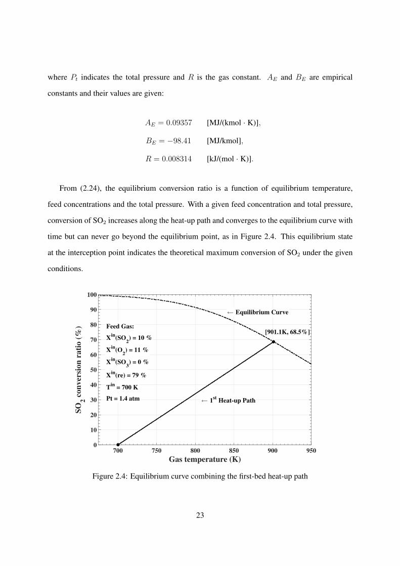
From (2.24), the equilibrium conversion ratio is a function of equilibrium temperature,

feed concentrations and the total pressure. With a given feed concentration and total pressure,

conversion of SO2 increases along the heat-up path and converges to the equilibrium curve with

time but can never go beyond the equilibrium point, as in Figure 2.4. This equilibrium state

at the interception point indicates the theoretical maximum conversion of SO2 under the given

conditions.

Gas temperature (K)

700 750 800 850 900 950

SO

2 c

on

ver

sion

ra

tio (

%)

0

10

20

30

40

50

60

70

80

90

100

Feed Gas:

Xin

(SO2) = 10 %

Xin

(O2) = 11 %

Xin

(SO3) = 0 %

Xin

(re) = 79 %

Tin

= 700 K

Pt = 1.4 atm← 1

st Heat-up Path

← Equilibrium Curve

[901.1K, 68.5%]

Figure 2.4: Equilibrium curve combining the first-bed heat-up path

23

2.3 Simulation

Gas temperature (K)

650 700 750 800 850 900 950

SO

2 c

on

ver

sion

rati

o (

%)

0

10

20

30

40

50

60

70

80

90

100

Feed Gas:

Xin

(SO2) = 10 %

Xin

(O2) = 11 %

Xin

(SO3) = 0 %

Xin

(re) = 79 %

Pt = 1.4 atm

1st

Heat-up Path →

← Equilibrium Curve2nd

Heat-up Path →

3rd

Heat-up Path

[890.2K, 71.6%]

[752.3K, 96.3%]

[688.2K, 99.1%]

Feed Gas:

Xin

(SO2) = 10 %

Xin

(O2) = 11 %

Xin

(SO3) = 0 %

Xin

(re) = 79 %

Pt = 1.4 atm

[901.1K, 68.5%]

[775.5K, 94.3%]

[712K, 98.4%]

Tin

= 680 K

Tin

= 700 K

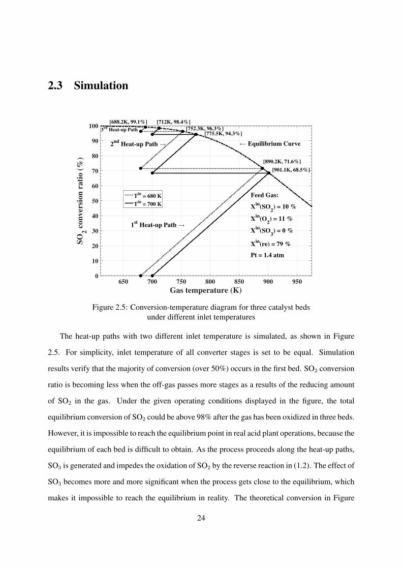
Figure 2.5: Conversion-temperature diagram for three catalyst bedsunder different inlet temperatures

The heat-up paths with two different inlet temperature is simulated, as shown in Figure

2.5. For simplicity, inlet temperature of all converter stages is set to be equal. Simulation

results verify that the majority of conversion (over 50%) occurs in the first bed. SO2 conversion

ratio is becoming less when the off-gas passes more stages as a results of the reducing amount

of SO2 in the gas. Under the given operating conditions displayed in the figure, the total

equilibrium conversion of SO2 could be above 98% after the gas has been oxidized in three beds.

However, it is impossible to reach the equilibrium point in real acid plant operations, because the

equilibrium of each bed is difficult to obtain. As the process proceeds along the heat-up paths,

SO3 is generated and impedes the oxidation of SO2 by the reverse reaction in (1.2). The effect of

SO3 becomes more and more significant when the process gets close to the equilibrium, which

makes it impossible to reach the equilibrium in reality. The theoretical conversion in Figure

24

2.5 provides the theoretical maximum conversion of the converter but cannot be obtained in

industrial operations. From Figure 2.5, it is noticed that a lower initial temperature is in favor

of a higher equilibrium conversion ratio and a lower equilibrium temperature. This equilibrium

conversion advantage gets less apparent after the gas passes more beds. Lower inlet temperature

is preferred for SO2 conversion, but the lower limit of the inlet gas temperature is always

determined by the catalyst ignition temperature, for example, ∼635K for the typical V2O5-

K2SO4 type of catalyst. In order to decrease the lower limit of inlet temperature, a new Cs-

promoted type of catalyst is found helpful by replacing the catalyst component K2SO4 with

cesium sulfate (Cs2SO4) (Schlesinger et al., 2011).

Gas temperature (K)

650 700 750 800 850 900 950

SO

2 c

on

ver

sion

rati

o (

%)

0

10

20

30

40

50

60

70

80

90

100

Feed Gas:

Xin

(O2)/X

in(SO

2) = 1.1

Xin

(SO3) = 0 %

Tin

= 700 K

Pt = 1.4 atm

1st

Heat-up Path →

← Equilibrium Curve2nd

Heat-up Path →

3rd

Heat-up Path

[901.1K, 68.5%]

[775.5K, 94.3%]

[712K, 98.4%]

Feed Gas:

Xin

(O2)/X

in(SO

2) = 1.1

Xin

(SO3) = 0 %

Tin

= 700 K

Pt = 1.4 atm

[912.2K, 66.2%]

[786.9K, 93.4%]

[715.9K, 98.4%]

Xin

(SO2) = 10 %

Xin

(SO2) = 11 %

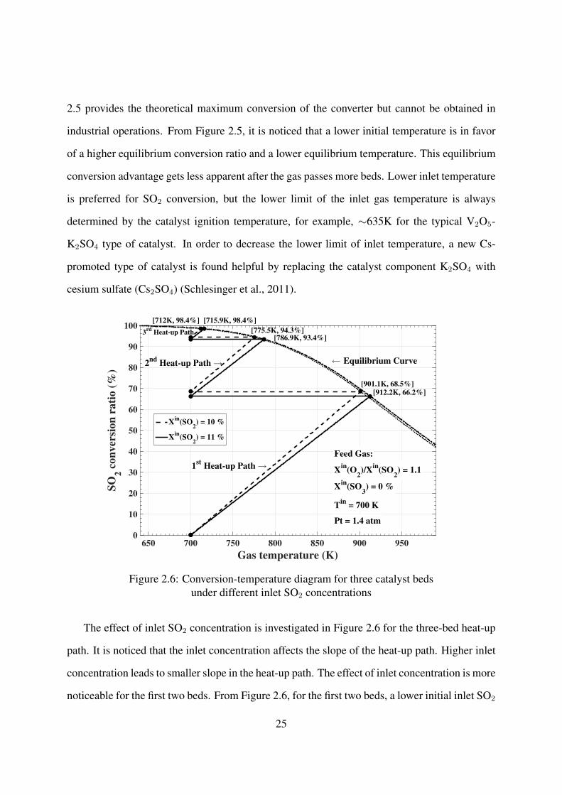
Figure 2.6: Conversion-temperature diagram for three catalyst bedsunder different inlet SO2 concentrations

The effect of inlet SO2 concentration is investigated in Figure 2.6 for the three-bed heat-up

path. It is noticed that the inlet concentration affects the slope of the heat-up path. Higher inlet

concentration leads to smaller slope in the heat-up path. The effect of inlet concentration is more

noticeable for the first two beds. From Figure 2.6, for the first two beds, a lower initial inlet SO2

25

concentration results in a higher equilibrium conversion but a lower equilibrium temperature.

For the third bed, the effect of inlet concentration on SO2 conversion becomes negligible. Even

though lower inlet SO2 concentration has a larger equilibrium conversion, an adequate SO2

concentration is required in the industrial operation in order to maintain an initial high reaction

rate.

Gas temperature (K)

700 750 800 850 900 950

SO

2 c

on

ver

sio

n r

ati

o (

%)

0

10

20

30

40

50

60

70

80

90

100

Feed Gas:

Xin

(SO2) = 10 %

Xin

(O2) = 11 %

Xin

(SO3) = 0 %

Xin

(re) = 79 %

Tin

= 700 K

← 1st

Heat-up Path

← Equilibrium Curve

[904.1K, 66.8%]

Feed Gas:

Xin

(SO2) = 10 %

Xin

(O2) = 11 %

Xin

(SO3) = 0 %

Xin

(re) = 79 %

Tin

= 700 K

[905.3K, 67.2%]

Pt = 1.3 atm

Pt = 1.4 atm

Figure 2.7: Conversion-temperature diagram for the first bedunder different gas pressures

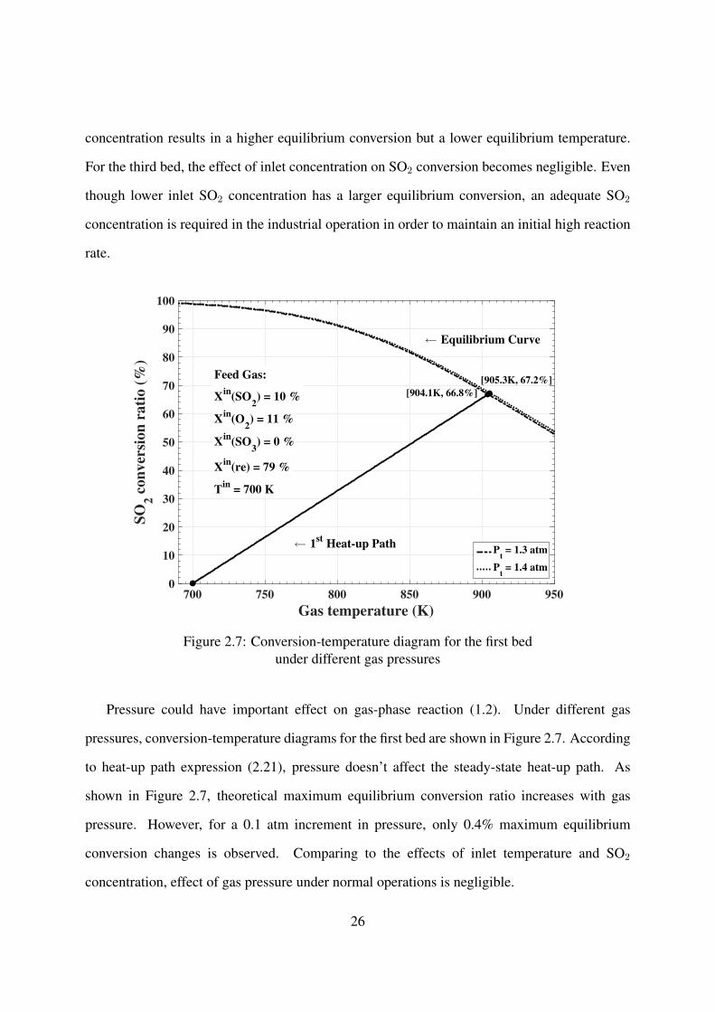
Pressure could have important effect on gas-phase reaction (1.2). Under different gas

pressures, conversion-temperature diagrams for the first bed are shown in Figure 2.7. According

to heat-up path expression (2.21), pressure doesn’t affect the steady-state heat-up path. As

shown in Figure 2.7, theoretical maximum equilibrium conversion ratio increases with gas

pressure. However, for a 0.1 atm increment in pressure, only 0.4% maximum equilibrium

conversion changes is observed. Comparing to the effects of inlet temperature and SO2

concentration, effect of gas pressure under normal operations is negligible.

26

2.4 Summary

In this chapter, a steady-state model of the catalytic SO2 converter is derived by applying

steady-state mass and energy balances. SO2 conversion ratio is defined and introduced. SO2

conversion ratio defines the percentage of oxidized SO2 over the feed SO2, and can serve as a

key performance indicator for the given converter. Based on steady-state model, the relation

between conversion ratio and gas temperature is obtained. The graphic representation of the

steady-state relation, termed as heat-up path, describes how gas temperature affects the SO2

conversion and provides an important base for dynamic modelling in the following chapters.

The heat-up path indicates that the conversion ratio increases with gas temperature along

the approximately linear path. With SO2 conversion ratio building up, more SO2 is converted

to SO3. Once the net reaction rate of reaction (1.2) gets zero, equilibrium of the reaction is

obtained and SO2 conversion stops. Interception of heat-up path and the equilibrium curve

shows the equilibrium state under given feed conditions. This equilibrium state indicates the

potential maximum SO2 conversion that a converter can achieve. As the growing production

of SO3 impedes the consumption SO2, conversion slows down when the reaction approaches

equilibrium.

Simulations are performed to investigate the effect of inlet SO2 concentration and gas

temperature on the multi-stage heat-up path and equilibrium SO2 conversion. It shows that

the inlet temperature affects the intercept of the heat-up path and the feed SO2 concentration

affects the slope of the path. From the simulation results, a lower inlet temperature and SO2

concentration are in favour to achieve a higher equilibrium conversion. However, the inlet gas

temperature is always limited by the catalyst activation temperature. To allow reaction (1.2)

to start, the inlet gas temperature has to be over the catalyst activation temperature. As for

inlet SO2, a low SO2 concentration leads to slow reaction and is not desirable for efficient SO2

conversion in the acid plant.

27

Chapter 3

Mathematical Soft Sensors

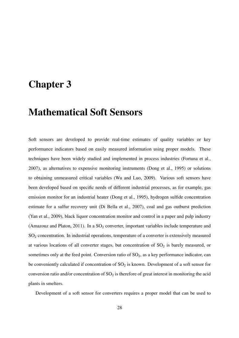
Soft sensors are developed to provide real-time estimates of quality variables or key

performance indicators based on easily measured information using proper models. These

techniques have been widely studied and implemented in process industries (Fortuna et al.,

2007), as alternatives to expensive monitoring instruments (Dong et al., 1995) or solutions

to obtaining unmeasured critical variables (Wu and Luo, 2009). Various soft sensors have

been developed based on specific needs of different industrial processes, as for example, gas

emission monitor for an industrial heater (Dong et al., 1995), hydrogen sulfide concentration

estimate for a sulfur recovery unit (Di Bella et al., 2007), coal and gas outburst prediction

(Yan et al., 2009), black liquor concentration monitor and control in a paper and pulp industry

(Amazouz and Platon, 2011). In a SO2 converter, important variables include temperature and

SO2 concentration. In industrial operations, temperature of a converter is extensively measured

at various locations of all converter stages, but concentration of SO2 is barely measured, or

sometimes only at the feed point. Conversion ratio of SO2, as a key performance indicator, can

be conveniently calculated if concentration of SO2 is known. Development of a soft sensor for

conversion ratio and/or concentration of SO2 is therefore of great interest in monitoring the acid

plants in smelters.

Development of a soft sensor for converters requires a proper model that can be used to

28

estimate the conversion ratio and concentration of SO2. Although modelling of the converters

have been investigated by many researchers (Snyder and Subramaniam, 1993; Hong et al.,

1997; Xiao and Yuan, 1996; Wu et al., 1996), most of these models were not developed for

the converters in industrial smelters. Even for dynamic models developed for the converters in

industrial smelters, they may not be able to serve as soft sensors due to model-plant mismatch,

a large number of unknown parameters as well as difficulty in parameter estimations fit with

the industrial operations. A steady-state model can be reliably built with known parameters

but it cannot be used as real-time soft sensor due to dynamic characteristics of the industrial

process. In this chapter, mathematical soft sensors are developed based on modification of the

steady-state models derived in Chapter 2 and real-time industrial data analysis. The obtained

soft sensors are simple to implement and can provide real-time estimates for the conversion

ratio and concentration of SO2 in a SO2 converter.

3.1 Soft Sensors Development and Application

3.1.1 Steady-State Relations

In Chapter 2, based on the steady-state mass and energy balances, heat-up path of a catalytic

SO2 converter is proposed and the SO2 conversion ratio is obtained as:

Φ =(X in

SO2kp,SO2 +X in

O2kp,O2 +X in

SO3kp,SO3 +X in

rekp,N2)(T − T in)[(kp,SO2 +

1

2kp,O2 − kp,SO3

)T +

(bSO2 +

1

2bO2 − bSO3

)]X inSO2

(3.1)

From Equation (3.1), it is noticed that SO2 conversion Φ can be calculated and obtained when

feed gas concentrations, inlet and outlet temperatures are available. Besides, as described in

Equation (2.13), that is,

XSO2 =(1− Φ)X in

SO2

1− 1

2ΦX in

SO2

, (3.2)

29

the outlet SO2 concentration is derived when Φ is achieved from Equation (3.1) and collected

measurements.

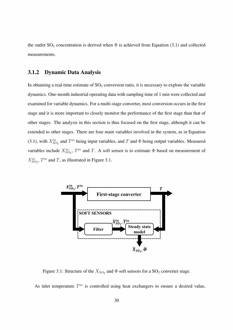
3.1.2 Dynamic Data Analysis

In obtaining a real-time estimate of SO2 conversion ratio, it is necessary to explore the variable

dynamics. One-month industrial operating data with sampling time of 1 min were collected and

examined for variable dynamics. For a multi-stage converter, most conversion occurs in the first

stage and it is more important to closely monitor the performance of the first stage than that of

other stages. The analysis in this section is thus focused on the first stage, although it can be

extended to other stages. There are four main variables involved in the system, as in Equation

(3.1), with X inSO2

and T in being input variables, and T and Φ being output variables. Measured

variables include X inSO2

, T in and T . A soft sensor is to estimate Φ based on measurement of

X inSO2

, T in and T , as illustrated in Figure 3.1.

Steady state model

Filter

First-stage converter

SOFT SENSORS

Figure 3.1: Structure of the XSO2 and Φ soft sensors for a SO2 converter stage.

As inlet temperature T in is controlled using heat exchangers to ensure a desired value,

30

Time (min)

0 20 40 60 80 100 120 140

Fee

d S

O2 m

ola

r

fract

ion

(%

)

6

8

10

12

Time (min)

0 20 40 60 80 100 120 140

Ou

tlet

tem

per

atu

re (

K)

840

860

880

900

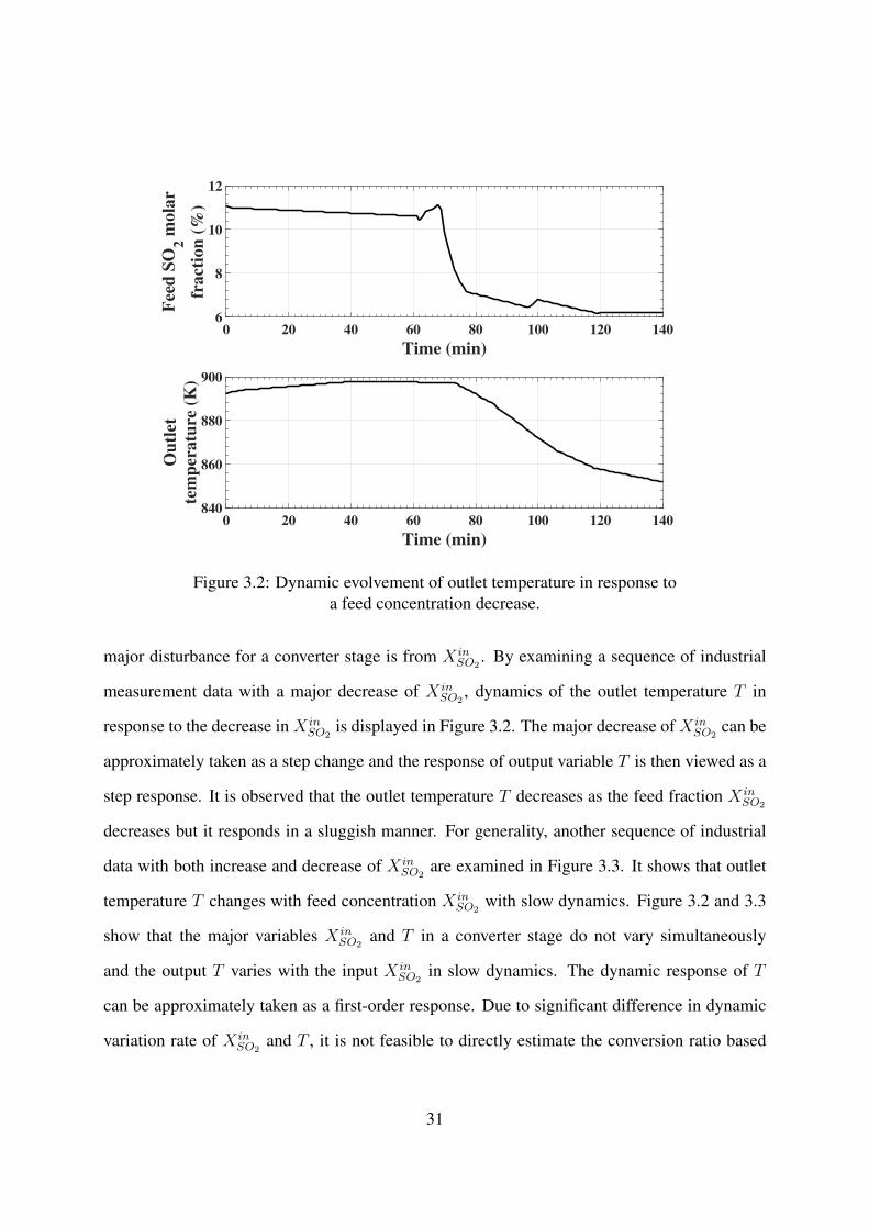
Figure 3.2: Dynamic evolvement of outlet temperature in response toa feed concentration decrease.

major disturbance for a converter stage is from X inSO2

. By examining a sequence of industrial

measurement data with a major decrease of X inSO2

, dynamics of the outlet temperature T in

response to the decrease in X inSO2

is displayed in Figure 3.2. The major decrease of X inSO2

can be

approximately taken as a step change and the response of output variable T is then viewed as a

step response. It is observed that the outlet temperature T decreases as the feed fraction X inSO2

decreases but it responds in a sluggish manner. For generality, another sequence of industrial

data with both increase and decrease of X inSO2

are examined in Figure 3.3. It shows that outlet

temperature T changes with feed concentration X inSO2

with slow dynamics. Figure 3.2 and 3.3

show that the major variables X inSO2

and T in a converter stage do not vary simultaneously

and the output T varies with the input X inSO2

in slow dynamics. The dynamic response of T

can be approximately taken as a first-order response. Due to significant difference in dynamic

variation rate of X inSO2

and T , it is not feasible to directly estimate the conversion ratio based

31

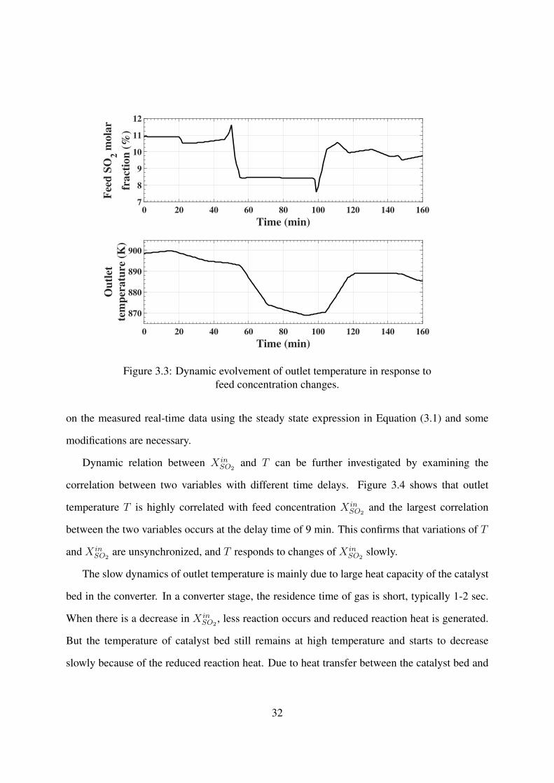
Time (min)

0 20 40 60 80 100 120 140 160

Fee

d S

O2 m

ola

r

fract

ion

(%

)

7

8

9

10

11

12

Time (min)

0 20 40 60 80 100 120 140 160

Ou

tlet

tem

per

atu

re (

K)

870

880

890

900

Figure 3.3: Dynamic evolvement of outlet temperature in response tofeed concentration changes.

on the measured real-time data using the steady state expression in Equation (3.1) and some

modifications are necessary.

Dynamic relation between X inSO2

and T can be further investigated by examining the

correlation between two variables with different time delays. Figure 3.4 shows that outlet

temperature T is highly correlated with feed concentration X inSO2

and the largest correlation

between the two variables occurs at the delay time of 9 min. This confirms that variations of T

and X inSO2

are unsynchronized, and T responds to changes of X inSO2

slowly.

The slow dynamics of outlet temperature is mainly due to large heat capacity of the catalyst

bed in the converter. In a converter stage, the residence time of gas is short, typically 1-2 sec.

When there is a decrease in X inSO2

, less reaction occurs and reduced reaction heat is generated.

But the temperature of catalyst bed still remains at high temperature and starts to decrease

slowly because of the reduced reaction heat. Due to heat transfer between the catalyst bed and

32

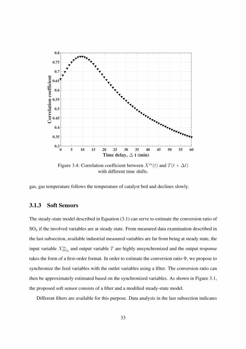
Time delay, ∆ t (min)0 5 10 15 20 25 30 35 40 45 50 55 60

Co

rrel

ati

on

co

effi

cien

t

0.3

0.35

0.4

0.45

0.5

0.55

0.6

0.65

0.7

0.75

0.8

Figure 3.4: Correlation coefficient between X in(t) and T (t+ ∆t)with different time shifts.

gas, gas temperature follows the temperature of catalyst bed and declines slowly.

3.1.3 Soft Sensors

The steady-state model described in Equation (3.1) can serve to estimate the conversion ratio of

SO2 if the involved variables are at steady state. From measured data examination described in

the last subsection, available industrial measured variables are far from being at steady state, the

input variable X inSO2

and output variable T are highly unsynchronized and the output response

takes the form of a first-order format. In order to estimate the conversion ratio Φ, we propose to

synchronize the feed variables with the outlet variables using a filter. The conversion ratio can

then be approximately estimated based on the synchronized variables. As shown in Figure 3.1,

the proposed soft sensor consists of a filter and a modified steady-state model.

Different filters are available for this purpose. Data analysis in the last subsection indicates

33

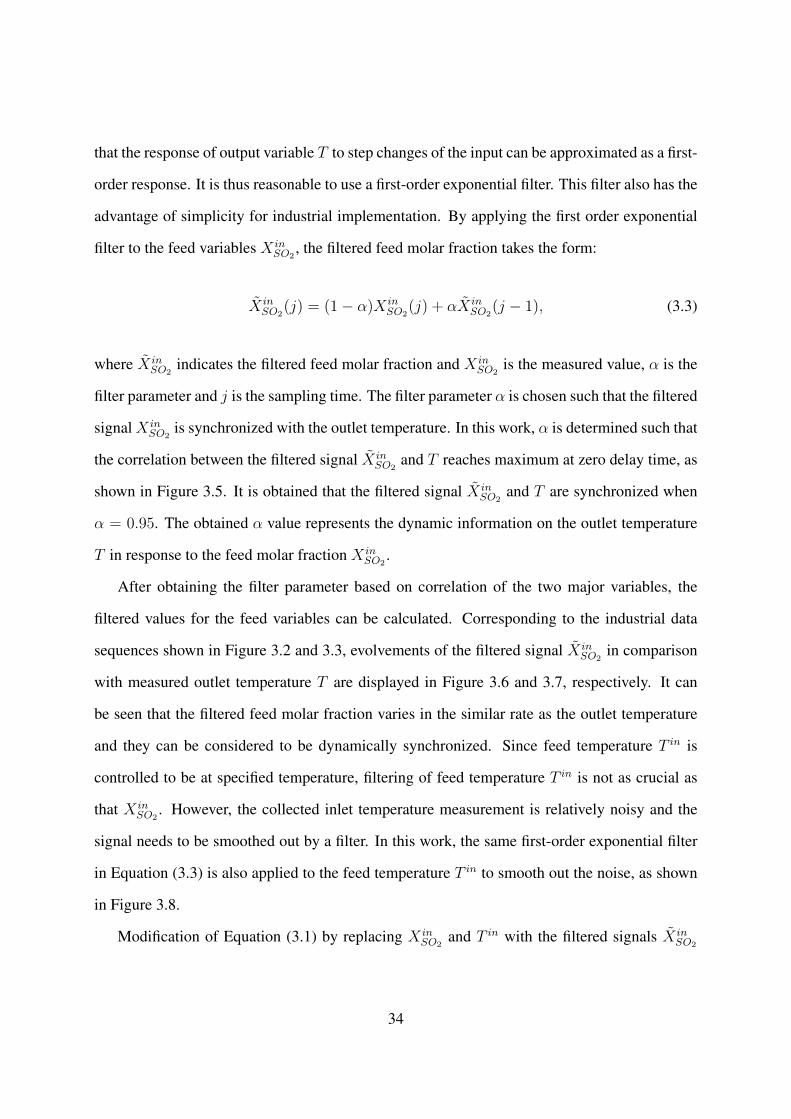
that the response of output variable T to step changes of the input can be approximated as a first-

order response. It is thus reasonable to use a first-order exponential filter. This filter also has the

advantage of simplicity for industrial implementation. By applying the first order exponential

filter to the feed variables X inSO2

, the filtered feed molar fraction takes the form:

X inSO2

(j) = (1− α)X inSO2

(j) + αX inSO2

(j − 1), (3.3)

where X inSO2

indicates the filtered feed molar fraction and X inSO2

is the measured value, α is the

filter parameter and j is the sampling time. The filter parameter α is chosen such that the filtered

signalX inSO2

is synchronized with the outlet temperature. In this work, α is determined such that

the correlation between the filtered signal X inSO2

and T reaches maximum at zero delay time, as

shown in Figure 3.5. It is obtained that the filtered signal X inSO2

and T are synchronized when

α = 0.95. The obtained α value represents the dynamic information on the outlet temperature

T in response to the feed molar fraction X inSO2

.

After obtaining the filter parameter based on correlation of the two major variables, the

filtered values for the feed variables can be calculated. Corresponding to the industrial data

sequences shown in Figure 3.2 and 3.3, evolvements of the filtered signal X inSO2

in comparison

with measured outlet temperature T are displayed in Figure 3.6 and 3.7, respectively. It can

be seen that the filtered feed molar fraction varies in the similar rate as the outlet temperature

and they can be considered to be dynamically synchronized. Since feed temperature T in is

controlled to be at specified temperature, filtering of feed temperature T in is not as crucial as

that X inSO2

. However, the collected inlet temperature measurement is relatively noisy and the

signal needs to be smoothed out by a filter. In this work, the same first-order exponential filter

in Equation (3.3) is also applied to the feed temperature T in to smooth out the noise, as shown

in Figure 3.8.

Modification of Equation (3.1) by replacing X inSO2

and T in with the filtered signals X inSO2

34

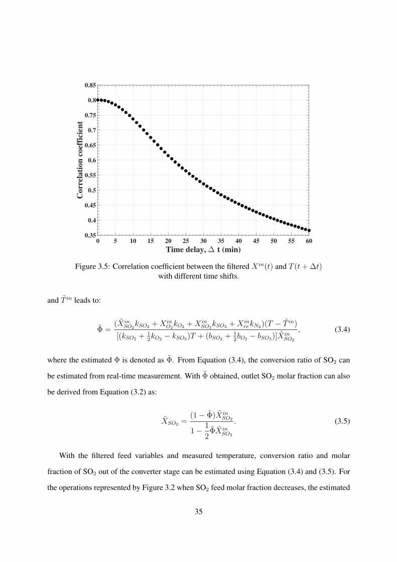
Time delay, ∆ t (min)0 5 10 15 20 25 30 35 40 45 50 55 60

Co

rrel

ati

on

co

effi

cien

t

0.35

0.4

0.45

0.5

0.55

0.6

0.65

0.7

0.75

0.8

0.85

Figure 3.5: Correlation coefficient between the filtered X in(t) and T (t+ ∆t)with different time shifts.

and T in leads to:

Φ =(X in

SO2kSO2 +X in

O2kO2 +X in

SO3kSO3 +X in

rekN2)(T − T in)

[(kSO2 + 12kO2 − kSO3)T + (bSO2 + 1

2bO2 − bSO3)]X

inSO2

, (3.4)

where the estimated Φ is denoted as Φ. From Equation (3.4), the conversion ratio of SO2 can

be estimated from real-time measurement. With Φ obtained, outlet SO2 molar fraction can also

be derived from Equation (3.2) as:

XSO2 =(1− Φ)X in

SO2

1− 1

2ΦX in

SO2

. (3.5)

With the filtered feed variables and measured temperature, conversion ratio and molar

fraction of SO2 out of the converter stage can be estimated using Equation (3.4) and (3.5). For

the operations represented by Figure 3.2 when SO2 feed molar fraction decreases, the estimated

35

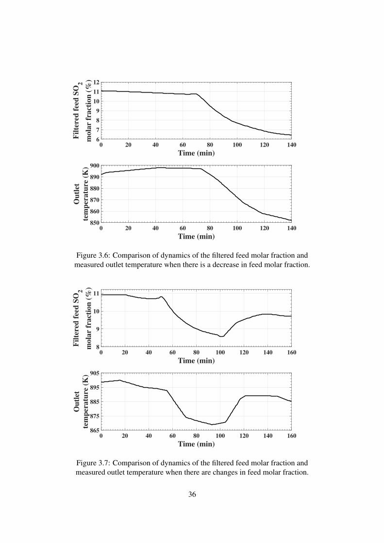
Time (min)

0 20 40 60 80 100 120 140

Fil

tere

d f

eed

SO

2

mola

r fr

act

ion

(%

)

6

7

8

9

10

11

12

Time (min)

0 20 40 60 80 100 120 140

Ou

tlet

tem

per

atu

re (

K)

850

860

870

880

890

900

Figure 3.6: Comparison of dynamics of the filtered feed molar fraction andmeasured outlet temperature when there is a decrease in feed molar fraction.

Time (min)

0 20 40 60 80 100 120 140 160

Fil

tere

d f

eed

SO

2

mola

r fr

act

ion

(%

)

8

9

10

11

Time (min)

0 20 40 60 80 100 120 140 160

Ou

tlet

tem

per

atu

re (

K)

865

875

885

895

905

Figure 3.7: Comparison of dynamics of the filtered feed molar fraction andmeasured outlet temperature when there are changes in feed molar fraction.

36

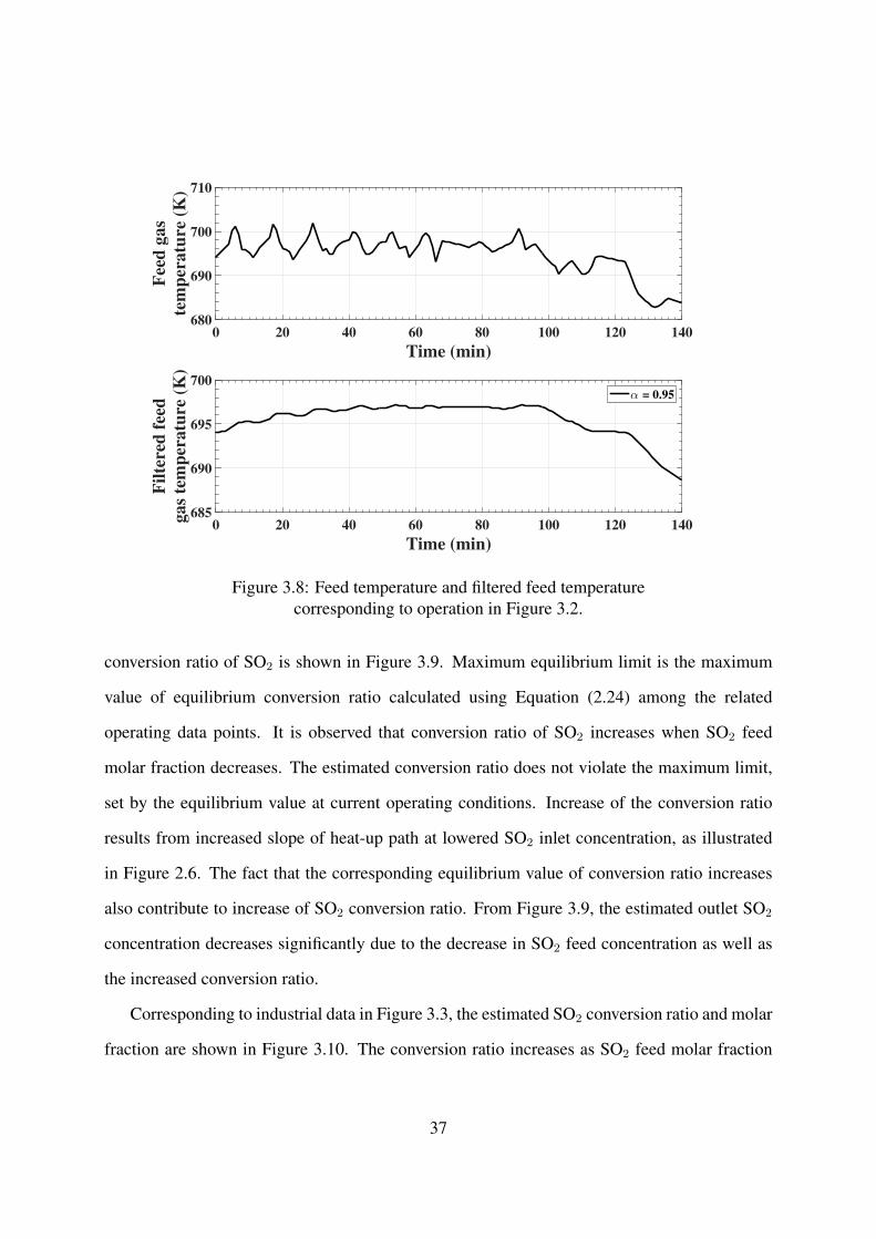
Time (min)

0 20 40 60 80 100 120 140

Fee

d g

as

tem

per

atu

re (

K)

680

690

700

710

Time (min)

0 20 40 60 80 100 120 140

Fil

tere

d f

eed

ga

s te

mp

era

ture

(K

)

685

690

695

700α = 0.95

Figure 3.8: Feed temperature and filtered feed temperaturecorresponding to operation in Figure 3.2.

conversion ratio of SO2 is shown in Figure 3.9. Maximum equilibrium limit is the maximum

value of equilibrium conversion ratio calculated using Equation (2.24) among the related

operating data points. It is observed that conversion ratio of SO2 increases when SO2 feed

molar fraction decreases. The estimated conversion ratio does not violate the maximum limit,

set by the equilibrium value at current operating conditions. Increase of the conversion ratio

results from increased slope of heat-up path at lowered SO2 inlet concentration, as illustrated

in Figure 2.6. The fact that the corresponding equilibrium value of conversion ratio increases

also contribute to increase of SO2 conversion ratio. From Figure 3.9, the estimated outlet SO2

concentration decreases significantly due to the decrease in SO2 feed concentration as well as

the increased conversion ratio.

Corresponding to industrial data in Figure 3.3, the estimated SO2 conversion ratio and molar

fraction are shown in Figure 3.10. The conversion ratio increases as SO2 feed molar fraction

37

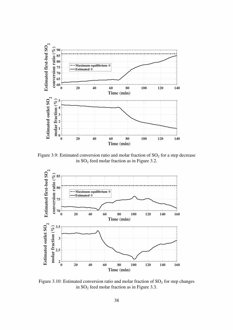
Time (min)

0 20 40 60 80 100 120 140Est

imate

d o

utl

et S

O2

mola

r fr

act

ion

(%

)

0

1

2

3

4

5

Time (min)

0 20 40 60 80 100 120 140Est

imate

d f

irst

-bed

SO

2

con

ver

sion

rati

o (

%)

60

65

70

75

80

85

90

Maximum equilibrium Φ

Estimated Φ

Figure 3.9: Estimated conversion ratio and molar fraction of SO2 for a step decreasein SO2 feed molar fraction as in Figure 3.2.

Time (min)

0 20 40 60 80 100 120 140 160Est

imate

d o

utl

et S

O2

mola

r fr

act

ion

(%

)

2

2.5

3

3.5

Time (min)

0 20 40 60 80 100 120 140 160Est

imate

d f

irst

-bed

SO

2

con

ver

sion

rati

o (

%)

70

75

80

85

Maximum equilibrium Φ

Estimated Φ

Figure 3.10: Estimated conversion ratio and molar fraction of SO2 for step changesin SO2 feed molar fraction as in Figure 3.3.

38

decreases while it decreases as SO2 feed increases, as suggested by the first-bed heat-up path

in Figure 2.6. The estimated SO2 outlet molar fraction varies in the same direction as SO2 feed

molar fraction and it increases as SO2 feed molar fraction increases, as discussed before for

Figure 3.9.

The proposed soft sensor for SO2 conversion ratio is compared with the estimate based

solely on the steady-state model Equation (3.1). Figure 3.11 displays a comparison of the

conversion ratio for the data with a step decrease of SO2 feed molar fraction as in Figure 3.2.

It is clear that the estimated conversion ratio based solely on the steady-state model violates

the maximum equilibrium value when a sharp decrease in SO2 feed molar fraction occurs. The

proposed soft sensor generates an acceptable real-time estimate for SO2 conversion ratio. Most

available soft sensor approaches would not be applicable to this process because they usually

require to derive model parameters from an available database with measured conversion ratio.

Our proposed soft sensor provides a useful estimate on the important variable without requiring

additional industrial measurement.

Based on the reliable steady-state model, the estimates of conversion ratio Φ and molar

fraction XSO2 are expected to converge to their true steady-state value. Due to very short

residence time of gas in the converter stage, it is expected that conversion ratio Φ and

molar fraction XSO2 have a quick dynamic response to any changes in feed conditions. As

the estimates of these variables heavily rely on temperature measurement, slow dynamics

of temperature measurement limits the dynamics of the estimated variables and this may

make them slower than that of the true values. Despite the slow dynamics, the inferred

information for conversion ratio and outlet molar fraction is expected to track the true variation

of these variables in reasonable closeness. They can provide useful monitoring on converter

performance.

The proposed soft sensors can be used to estimate conversion ratio and molar fraction of

SO2 out of a converter stage. The estimated variables have not been validated with industrial

39

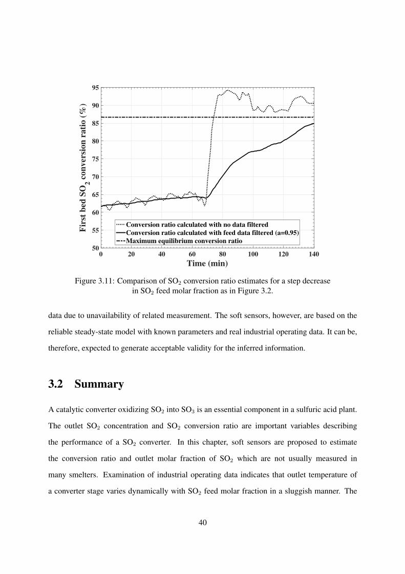
Time (min)

0 20 40 60 80 100 120 140

Fir

st b

ed S

O2 c

on

ver

sio

n r

ati

o (

%)

50

55

60

65

70

75

80

85

90

95

Conversion ratio calculated with no data filtered

Conversion ratio calculated with feed data filtered (a=0.95)

Maximum equilibrium conversion ratio

Figure 3.11: Comparison of SO2 conversion ratio estimates for a step decreasein SO2 feed molar fraction as in Figure 3.2.

data due to unavailability of related measurement. The soft sensors, however, are based on the

reliable steady-state model with known parameters and real industrial operating data. It can be,

therefore, expected to generate acceptable validity for the inferred information.

3.2 Summary

A catalytic converter oxidizing SO2 into SO3 is an essential component in a sulfuric acid plant.

The outlet SO2 concentration and SO2 conversion ratio are important variables describing

the performance of a SO2 converter. In this chapter, soft sensors are proposed to estimate

the conversion ratio and outlet molar fraction of SO2 which are not usually measured in

many smelters. Examination of industrial operating data indicates that outlet temperature of

a converter stage varies dynamically with SO2 feed molar fraction in a sluggish manner. The

40

two variables are highly correlated and the correlation coefficient reaches maximum at a delay

time of 9 minutes. Application of a first-order exponential filter to SO2 feed molar fraction

leads to the filtered signal that is synchronized with the outlet temperature. A reliable steady-

state model is developed for conversion ratio as a function of measured variables including

temperature and feed molar fraction. By replacing the original feed variables with the filtered

variables, the model generates useful estimation of the unmeasured variables.

41

Chapter 4

Dynamic Modelling of Sulfur Dioxide

Converter Using ODE

This chapter aims to develop a dynamic model for the catalytic SO2 converter in the acid plant of

an industrial smelter such that the model can well reflect the industrial operation but be simple

enough for the convenience of industrial applications. For the SO2 converters in the smelters,

conversion ratio of SO2 is a very important variable commonly used as a performance indicator.

In this chapter, SO2 conversion ratio is defined for the individual stage relative to the SO2 inlet

into each stage as well as that relative to the feed SO2 into the first stage of the converter.

Relation between the two types of the conversion ratio is formulated. For industrial uses, a

dynamic model is developed in the forms of both continuous ordinary differential equations

(ODE) and finite difference equations. The extent of SO2 oxidation in each stage is expressed

by the calculated equilibrium conversion ratio multiplied by a parameter. The parameter is

estimated from the industrial operating data and thus the obtained model can be readily adapted

to different industrial converters with various catalyst bed conditions. Simulation results show

that the obtained model fits well with the industrial data. Based on the model, process dynamics

are investigated for the converter in an industrial smelter.

42

4.1 SO2 Conversion Ratio

The SO2 catalytic converter performance indicator, SO2 conversion ratio has been defined in

Equation (2.6) and described in Chapter 2. In its definition, X inSO2

can be inlet SO2 molar

fraction to each bed or to the first bed of the converter. Depending on X inSO2

being used, two

types of SO2 conversion ratio can be calculated for each bed:

(1) the individual bed SO2 conversion ratio relative to the feed SO2 into each bed if X inSO2

indicates the SO2 inlet concentration into the corresponding bed;

(2) the overall converter SO2 conversion ratio for each bed relative to the feed SO2 into

the overall converter if X inSO2

indicates the SO2 inlet concentration to the first bed of the

converter.

Based on the definition of these two types of SO2 conversion ratio, the overall converter

conversion ratio Φt,k relative to the feed SO2 into the overall converter for each bed is related

to the individual bed conversion ratio Φk relative to the feed SO2 into the corresponding bed by


Φt,k = 1−k∏j=1

(1− Φj) , (4.1)

where k = 1, 2, 3, 4 representing the four converter stages. The overall converter SO2

conversion ratio Φt,k is usually referred to in the available literature (Davenport and King, 2006)

and discussed in Chapter 2. However, the individual bed SO2 conversion ratio Φk will be used

for modelling in this chapter.

Chapter 2 introduces the equilibrium state by combining the reaction equilibrium curve

with converter heat-up path. For equilibrium SO2 conversion ratio of each bed ΦEk , it can be

obtained by solving Equations (2.23) and Equations (2.24) when the inlet conditions of each

bed are applied, that is:

43

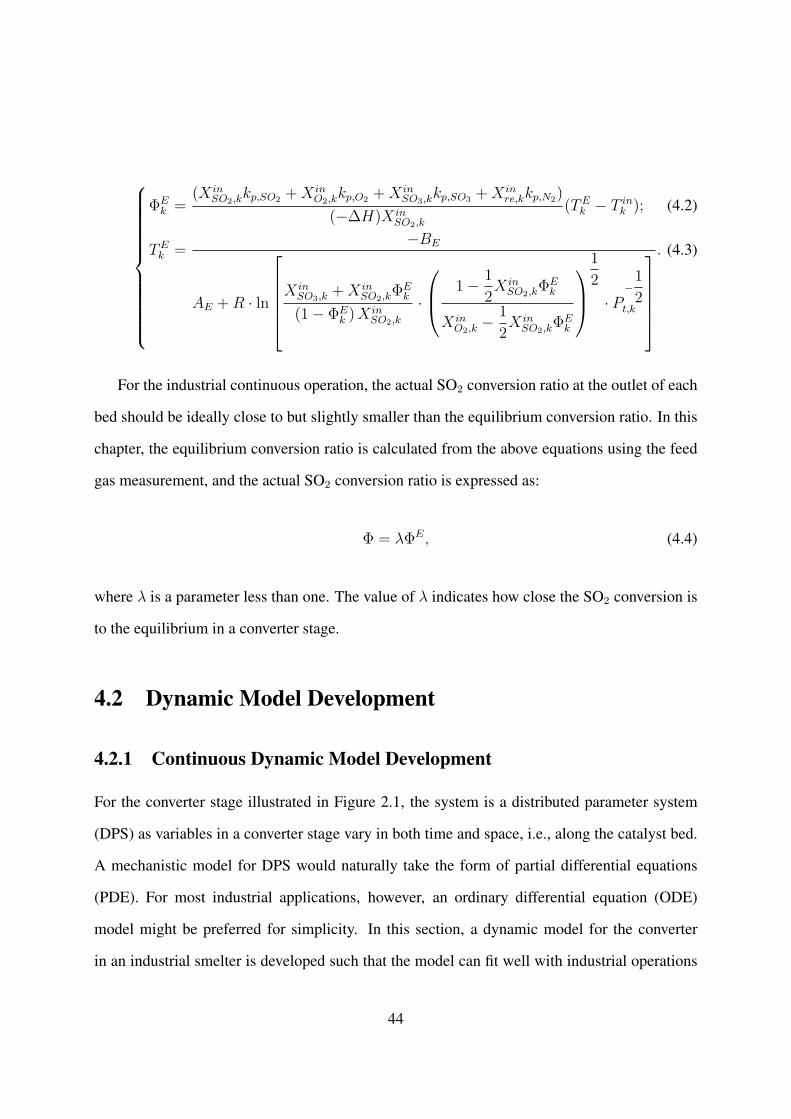
ΦEk =

(X inSO2,k

kp,SO2 +X inO2,k

kp,O2 +X inSO3,k

kp,SO3 +X inre,kkp,N2)

(−∆H)X inSO2,k

(TEk − T ink ); (4.2)

TEk =−BE

AE +R · ln

XinSO3,k

+X inSO2,k

ΦEk

(1− ΦEk )X in

SO2,k

·

1− 1

2X inSO2,k

ΦEk

X inO2,k− 1

2X inSO2,k

ΦEk

1

2

· P−

1

2t,k

. (4.3)

For the industrial continuous operation, the actual SO2 conversion ratio at the outlet of each

bed should be ideally close to but slightly smaller than the equilibrium conversion ratio. In this

chapter, the equilibrium conversion ratio is calculated from the above equations using the feed

gas measurement, and the actual SO2 conversion ratio is expressed as:

Φ = λΦE, (4.4)

where λ is a parameter less than one. The value of λ indicates how close the SO2 conversion is

to the equilibrium in a converter stage.

4.2 Dynamic Model Development

4.2.1 Continuous Dynamic Model Development

For the converter stage illustrated in Figure 2.1, the system is a distributed parameter system

(DPS) as variables in a converter stage vary in both time and space, i.e., along the catalyst bed.

A mechanistic model for DPS would naturally take the form of partial differential equations

(PDE). For most industrial applications, however, an ordinary differential equation (ODE)

model might be preferred for simplicity. In this section, a dynamic model for the converter

in an industrial smelter is developed such that the model can fit well with industrial operations

44

and be convenient for industrial applications. For this purpose, it is assumed that:

(1) the value of variables at the outlet of the converter stage is approximately equal to that

within the converter stage;

(2) the converter is considered to be adiabatic;

(3) temperature of the catalyst beds closely follows that of the gas.

Under these assumptions, a dynamic model can be developed based on mass and energy

balances:

ρgVgMg

dXSO2

dt=ρgQ

in

Mg

(X inSO2−XSO2

)− (1− 1

2XSO2)r, (4.5)

(ρgcp,gVg + ρcatcp,catVcat)dT

dt= ρgcp,gQ

in(T in − T

)+ (−∆H)r, (4.6)

where r [mol/min] indicates the consumption rate of SO2.

For the overall gas molecular weight, Mg, it is related with the gas compositions and can be

evaluated by applying the Gibbs-Dalton’s law (Shao et al., 2013):

Mg =∑i

(XiMi) , (4.7)

where i represents the gas components in the gas stream (SO2, O2, SO3 and N2). When the gas

stream is considered to be ideal gas mixture, the gas density ρg can be derived by:

ρg =PtMg

RT, (4.8)

where Pt is the total gas pressure. As for the heat capacity cp,g of the gas stream, it can be

obtained as described in Section 5.3.2.

The reaction kinetics for SO2 oxidation has been extensively studied and the available

expressions for the reaction rate are mostly from the lab test results (Froment and Bischoff,

1979; Kiss et al., 2010). For industrial systems, the reaction rate could be different due to

45

different combinations of catalysts and packing patterns. The available kinetic expressions may

not fit well with industrial systems or contain too many parameters that are hard to be estimated

from industrial operating data. In developing a model that can fit well with different industrial

converters, the model in Equation (4.6) should be further modified so that the model can be

applicable even if the reaction kinetics is not available.

Considering the fact that ρg � ρcat, the dynamics of XSO2 in Equation (4.5) are negligible

in comparison with those of T in Equation (4.6), that is, Equation (4.5) can be approximated as:

0 ≈ ρgQin

Mg

(X inSO2−XSO2

)− (1− 1

2XSO2)r, (4.9)

and

r =ρgQ

in

Mg

·X inSO2−XSO2

1− 1

2XSO2

. (4.10)

Using Equation (2.17), expression of reaction rate r in (4.10) can be rewritten as:

r =ρgQ

in

Mg

ΦX inSO2

. (4.11)

With the Equation (4.11) and the fact that ρg � ρcat, the model in Equation (4.6) is thus further

simplified:ρcatcp,catVcatρgcp,gQin

dT

dt= T in − T +X in

SO2Φ−∆H

cp,gMg

. (4.12)

Substituting (4.4) to (4.12), the model can also be represented as:

ρcatcp,catVcatρgcp,gQin

dT

dt= T in − T + λX in

SO2ΦE −∆H

cp,gMg

, (4.13)

where the equilibrium conversion ratio ΦE can be computed with the given feed conditions

through Equations (4.2) and (4.3). This model in (4.13) describes how gas temperature out of

a converter stage evolves under given feed conditions. The parameter λ needs to be estimated

46

from the industrial operating data and other parameters can be obtained based on the process

information.

4.2.2 Discrete-Time Model

For parameter estimation and industrial applications, a discrete-time model based on Equation

(4.13) is required. Defining

Vsp =ρcatcp,catVcat

ρgcp,g, (4.14)

Equation (4.13) can be rearranged as

dT

dt+Qin

VspT =

Qin

Vsp

(T in + λX in

SO2ΦE −∆H

cp,gMg

). (4.15)

If exp(Qin

Vspt)

is multiplied to both sides of Equation (4.15), it becomes

d

dt

[exp

(Qin

Vspt

)T

]= exp

(Qin

Vspt

)Qin

Vsp

(T in + λX in

SO2ΦE −∆H

cp,gMg

). (4.16)

For calculation convenience, feed conditions are not considered time-varied over the short

time period ∆t. In this case, applying integration from t to t+ ∆t to Equation (4.16), yields:

[exp

(Qin

Vspt

)T

]∣∣∣∣t+∆t

t

=

(T in + λX in

SO2ΦE −∆H

cp,gMg

)(exp

(Qin

Vspt

)∣∣∣∣t+∆t

t

), (4.17)

exp

[Qin

Vsp(t+ ∆t)

]T (t+ ∆t)− exp

(Qin

Vspt

)T (t)

=

(T in + λX in

SO2ΦE −∆H

cp,gMg

){exp

[Qin

Vsp(t+ ∆t)

]− exp

(Qin

Vspt

)}.

(4.18)

After rearrangement, a model regarding outlet temperature is derived:

T (t+ ∆t) = exp

(−Q

in

Vsp∆t

)T (t)

+

[1− exp

(−Q

in

Vsp∆t

)](T in + λX in

SO2ΦE −∆H

cp,gMg

),

(4.19)

47

that is,

Tk (j + 1) = exp

(− Qin

k (j)

Vsp,k(j)∆t

)Tk (j)

+

[1− exp

(− Qin

k (j)

Vsp,k(j)∆t

)][T ink (j) + λkX

inSO2,k

(j)ΦEk (j)

−∆H

cp,gMg

],

(4.20)

where j indicates the sampling time and k = 1, 2, 3, 4 representing the four converter stages.

The discrete-time model in (4.20) is convenient for parameter estimation and model validation

from the industrial discrete-time data. From the developed models, it can be seen that process

dynamics for the gas temperature is dominantly affected by the term Vsp/Qin - the larger term

implying the slower dynamics.

With given feed conditions for each stage, model in (4.13) and (4.20) can be used to predict

the gas temperature variations for the converter stages. The needed feed conditions include feed

gas temperature, gas composition and flowrate. In industrial practices, inlet gas temperatures

for all stages are often measured. For the feed compositions of the first stage, gas concentration

of SO2 is usually available, SO3 molar concentration is assumed zero, and oxygen concentration

can be assumed to be proportionally related with SO2 concentration according to (Davenport

and King, 2006). For the second, third and forth stages, however, feed compositions are often

not measured online and information may not be available. It is thus necessary to estimate the

inlet gas compositions for these later stages. Due to the fact that the gas compositions remain

the same through heat exchangers between the first three converter stages (as shown in Figure

1.2), feed gas concentration of the second and third beds is equal to the outlet gas concentration

from the preceding beds, i.e.,

X ini,k = Xi,k−1, (k = 2, 3, and i = SO2, O2, SO3, re). (4.21)

Equation (4.21) is not applicable to the fourth stage as the gas needs to pass an interpass SO3

absorption tower after the third stage. If SO3 is assumed to be completely removed in the

48

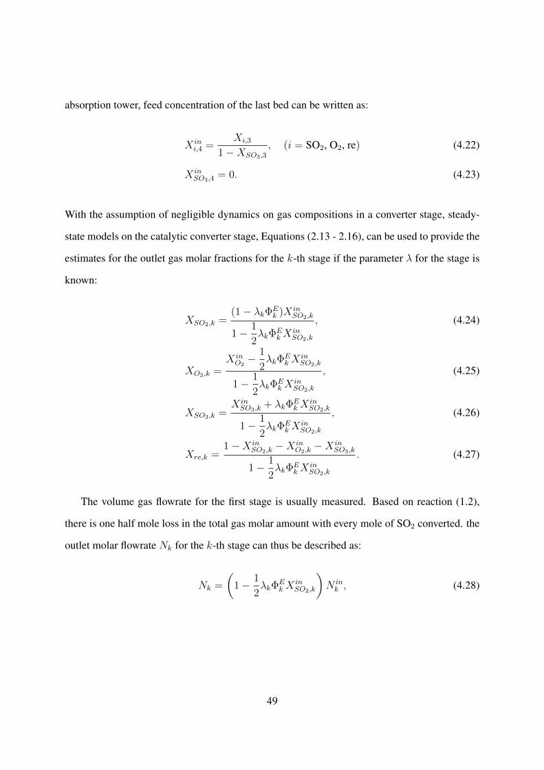
absorption tower, feed concentration of the last bed can be written as:

X ini,4 =

Xi,3

1−XSO3,3

, (i = SO2, O2, re) (4.22)

X inSO3,4

= 0. (4.23)

With the assumption of negligible dynamics on gas compositions in a converter stage, steady-

state models on the catalytic converter stage, Equations (2.13 - 2.16), can be used to provide the

estimates for the outlet gas molar fractions for the k-th stage if the parameter λ for the stage is

known:

XSO2,k =(1− λkΦE

k )X inSO2,k

1− 1

2λkΦE

kXinSO2,k

, (4.24)

XO2,k =X inO2− 1

2λkΦ

EkX

inSO2,k

1− 1

2λkΦE

kXinSO2,k

, (4.25)

XSO3,k =X inSO3,k

+ λkΦEkX

inSO2,k

1− 1

2λkΦE

kXinSO2,k

, (4.26)

Xre,k =1−X in

SO2,k−X in

O2,k−X in

SO3,k

1− 1

2λkΦE

kXinSO2,k

. (4.27)

The volume gas flowrate for the first stage is usually measured. Based on reaction (1.2),

there is one half mole loss in the total gas molar amount with every mole of SO2 converted. the

outlet molar flowrate Nk for the k-th stage can thus be described as:

Nk =

(1− 1

2λkΦ

EkX

inSO2,k

)N ink , (4.28)

49

where

N ink =

P ink Q

ink

RT ink, (4.29)

Nk =PkQk

RTk, (4.30)

if the ideal gas law is applied. Therefore, the volume flowrates of the second and third beds are

derived as:

Qink =

(1− 1

2λk−1ΦE

k−1XinSO2,k−1

)T ink P

ink−1Q

ink−1

T ink−1Pink

, (4.31)

where k = 2, 3. For the fourth bed, with a complete SO3 removal by the intermediate absorption

tower, its feed flowrate is:

Qin4 = (1−XSO3,3)

(1− 1

2λ3ΦE

3 XinSO2,3

)T in4 P in

3 Qin3

T in3 P in4

. (4.32)

With the given and estimated gas feed conditions for each bed, temperature and SO2

concentration (or conversion ratio) for the gas out of each bed can be predicted from the above

modelling equations (4.13) and (4.20).

4.3 Parameter Estimation

A dynamic model is developed for converter stages in the previous section. For the model to

reflect an industrial operation, the parameter λ needs to be estimated for each catalyst bed from

the industrial operating data. In this chapter, it is assumed that λ is a constant value for each

stage. The parameter λk is estimated by minimizing the following objective function:

minλk

Jk = minλk

∑j

[Tk(j)− Tk(j)

]2

, (k = 1, 2, 3, 4), (4.33)

50

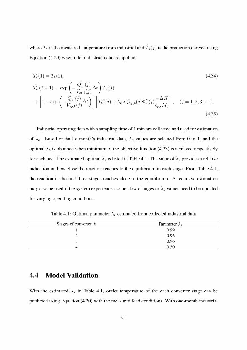
where Tk is the measured temperature from industrial and Tk(j) is the prediction derived using

Equation (4.20) when inlet industrial data are applied:

Tk(1) = Tk(1), (4.34)

Tk (j + 1) = exp

(− Qin

k (j)

Vsp,k(j)∆t

)Tk (j)

+

[1− exp

(− Qin

k (j)

Vsp,k(j)∆t

)][T ink (j) + λkX

inSO2,k

(j)ΦEk (j)

−∆H

cp,gMg

], (j = 1, 2, 3, · · · ).

(4.35)

Industrial operating data with a sampling time of 1 min are collected and used for estimation

of λk. Based on half a month’s industrial data, λk values are selected from 0 to 1, and the

optimal λk is obtained when minimum of the objective function (4.33) is achieved respectively

for each bed. The estimated optimal λk is listed in Table 4.1. The value of λk provides a relative

indication on how close the reaction reaches to the equilibrium in each stage. From Table 4.1,

the reaction in the first three stages reaches close to the equilibrium. A recursive estimation

may also be used if the system experiences some slow changes or λk values need to be updated

for varying operating conditions.

Table 4.1: Optimal parameter λk estimated from collected industrial data

Stages of converter, k Parameter λk1 0.992 0.963 0.964 0.30

4.4 Model Validation

With the estimated λk in Table 4.1, outlet temperature of the each converter stage can be

predicted using Equation (4.20) with the measured feed conditions. With one-month industrial

51

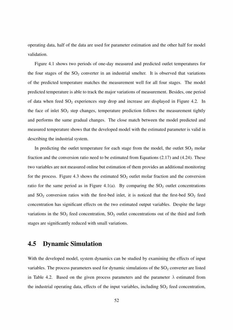
operating data, half of the data are used for parameter estimation and the other half for model

validation.

Figure 4.1 shows two periods of one-day measured and predicted outlet temperatures for

the four stages of the SO2 converter in an industrial smelter. It is observed that variations

of the predicted temperature matches the measurement well for all four stages. The model

predicted temperature is able to track the major variations of measurement. Besides, one period

of data when feed SO2 experiences step drop and increase are displayed in Figure 4.2. In

the face of inlet SO2 step changes, temperature prediction follows the measurement tightly

and performs the same gradual changes. The close match between the model predicted and

measured temperature shows that the developed model with the estimated parameter is valid in

describing the industrial system.

In predicting the outlet temperature for each stage from the model, the outlet SO2 molar

fraction and the conversion ratio need to be estimated from Equations (2.17) and (4.24). These

two variables are not measured online but estimation of them provides an additional monitoring

for the process. Figure 4.3 shows the estimated SO2 outlet molar fraction and the conversion

ratio for the same period as in Figure 4.1(a). By comparing the SO2 outlet concentrations

and SO2 conversion ratios with the first-bed inlet, it is noticed that the first-bed SO2 feed

concentration has significant effects on the two estimated output variables. Despite the large

variations in the SO2 feed concentration, SO2 outlet concentrations out of the third and forth

stages are significantly reduced with small variations.

4.5 Dynamic Simulation

With the developed model, system dynamics can be studied by examining the effects of input

variables. The process parameters used for dynamic simulations of the SO2 converter are listed

in Table 4.2. Based on the given process parameters and the parameter λ estimated from

the industrial operating data, effects of the input variables, including SO2 feed concentration,

52

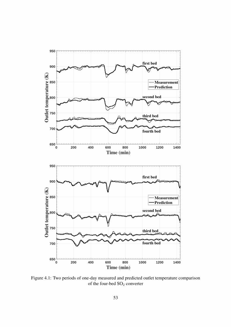
Time (min)0 200 400 600 800 1000 1200 1400

Ou

tlet

tem

per

atu

re (

K)

650

700

750

800

850

900

950

first bed

second bed

third bed

fourth bed

Measurement

Prediction

Time (min)0 200 400 600 800 1000 1200 1400

Ou

tlet

tem

per

atu

re (

K)

650

700

750

800

850

900

950

first bed

second bed

third bed

fourth bed

Measurement

Prediction

Figure 4.1: Two periods of one-day measured and predicted outlet temperature comparisonof the four-bed SO2 converter

53

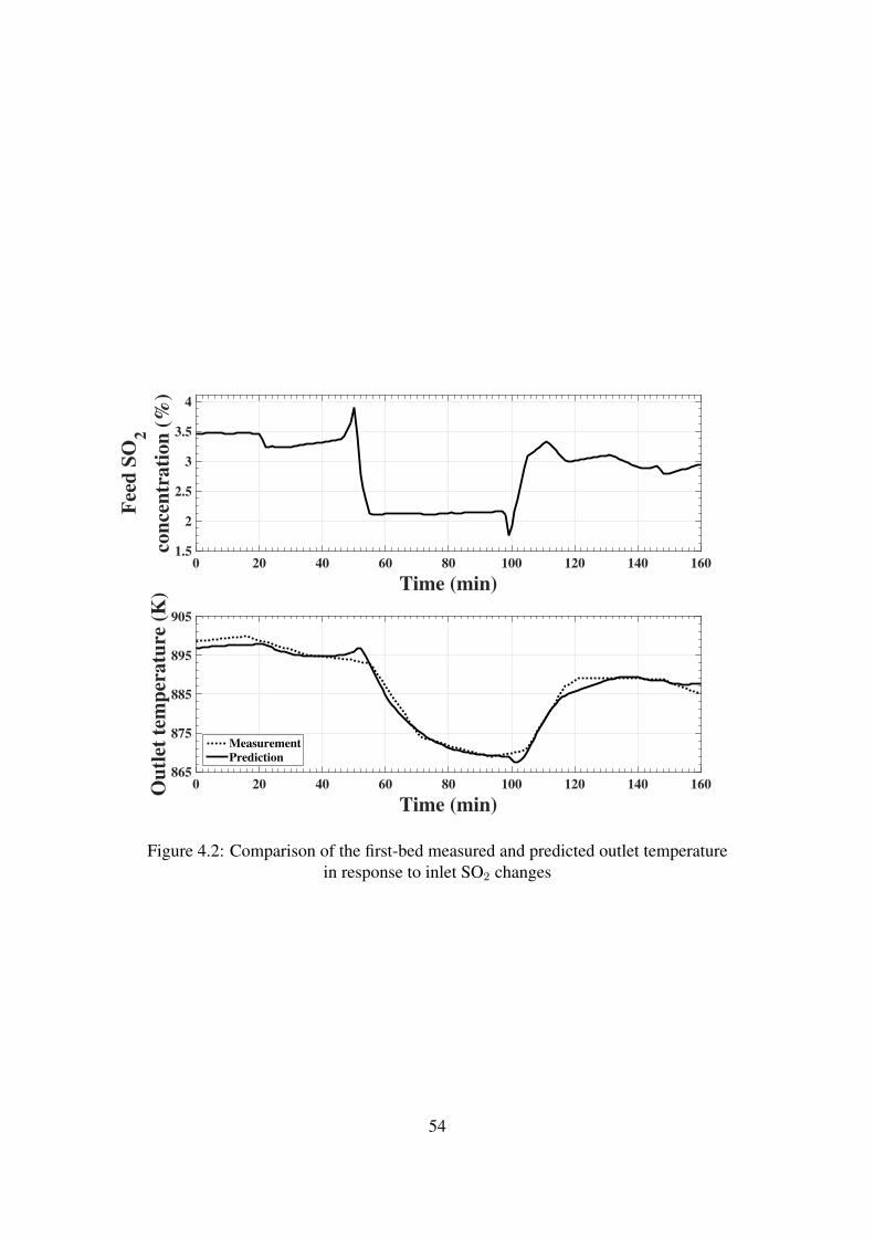
Time (min)0 20 40 60 80 100 120 140 160

Fee

d S

O2

con

cen

trati

on

(%

)

1.5

2

2.5

3

3.5

4

Time (min)0 20 40 60 80 100 120 140 160O

utl

et t

emp

eratu

re (

K)

865

875

885

895

905

Measurement

Prediction

Figure 4.2: Comparison of the first-bed measured and predicted outlet temperaturein response to inlet SO2 changes

54

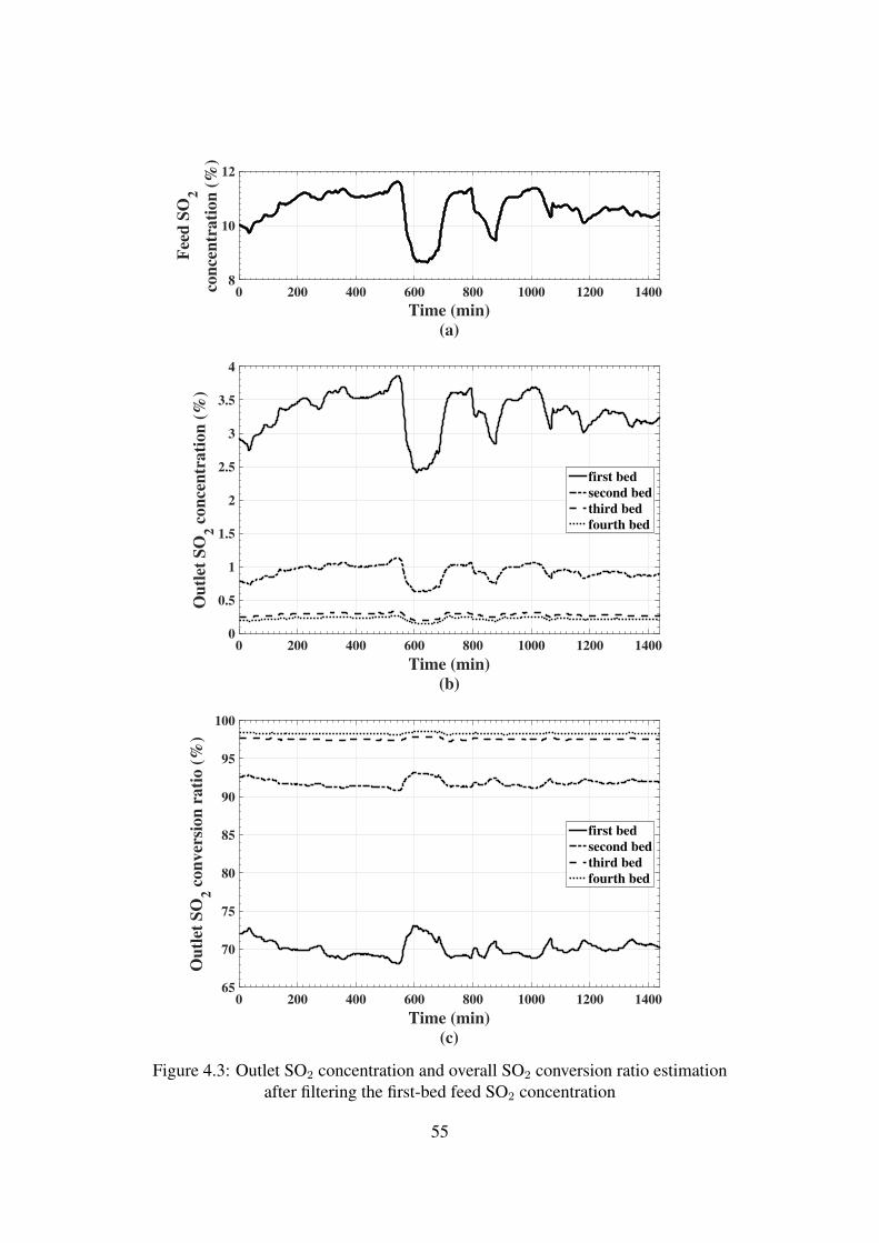
Time (min)

(a)

0 200 400 600 800 1000 1200 1400

Feed

SO

2

co

ncen

tra

tio

n (

%)

8

10

12

Time (min)

(b)

0 200 400 600 800 1000 1200 1400

Ou

tlet

SO

2 c

on

cen

tra

tio

n (

%)

0

0.5

1

1.5

2

2.5

3

3.5

4

first bed

second bed

third bed

fourth bed

Time (min)

(c)

0 200 400 600 800 1000 1200 1400

Ou

tlet

SO

2 c

on

versi

on

ra

tio

(%

)

65

70

75

80

85

90

95

100

first bed

second bed

third bed

fourth bed

Figure 4.3: Outlet SO2 concentration and overall SO2 conversion ratio estimationafter filtering the first-bed feed SO2 concentration

55

flowrate and the feed gas temperature, are investigated.

Table 4.2: Initial conditions and process parameters for dynamic simulations

Initial conditions Process parametersX inSO2,1 10 % V1 80 m3

X inO2,1 11 %a V2 96 m3

X inSO3,1 0 % V3 125 m3

T in 660 Kb V4 120 m3

Pt,1 1.4 atm ρcat,1 412 kg/m3




Qin1 194 km3/hr cp,cat 830 J/(kg·K)

a First-bed inlet O2 concentration is assumed to be 1.1XinSO2,1

(Davenport and King, 2006).b Inlet temperature for all stages is assumed to be the same for simulation simplicity.

SO2 feed concentration to the converter is an important disturbance input variable for the

converter in a smelter. A smelter generates offgas laden with SO2 and the gas is fed to an

acid plant for SO2 reduction. The offgas from the smelter may have large variations in SO2

concentration, which significantly raises the operational challenge for the acid plant in a smelter

in comparison with that using sulfur burning as its source gas. The effect of SO2 concentration

in the feed gas on the system dynamics of the converter is investigated by examining the step

response of the outlet temperature. Figure 4.4 displays the outlet temperature evolvements

of the four beds when the first-bed inlet SO2 molar fraction has a step increase from 10%

to 11%. It is observed that SO2 feed concentration in the source gas affects the outlet gas

temperature for all four stages and temperatures increase with the SO2 feed concentration. It is

thus important to control the feed concentration to be within a proper range so that over-heating

of the catalyst beds can be avoided while maintaining an efficient SO2 conversion. From Figure

4.4, the temperature increment resulting from the SO2 feed concentration increase is the largest

for the first bed and the increment reduces for the second bed, and only small temperature

increment is observed for the third and forth beds. This implies that most SO2 in the offgas is

converted in the first two stages, and only small amount of SO2 conversions occur in the third

56

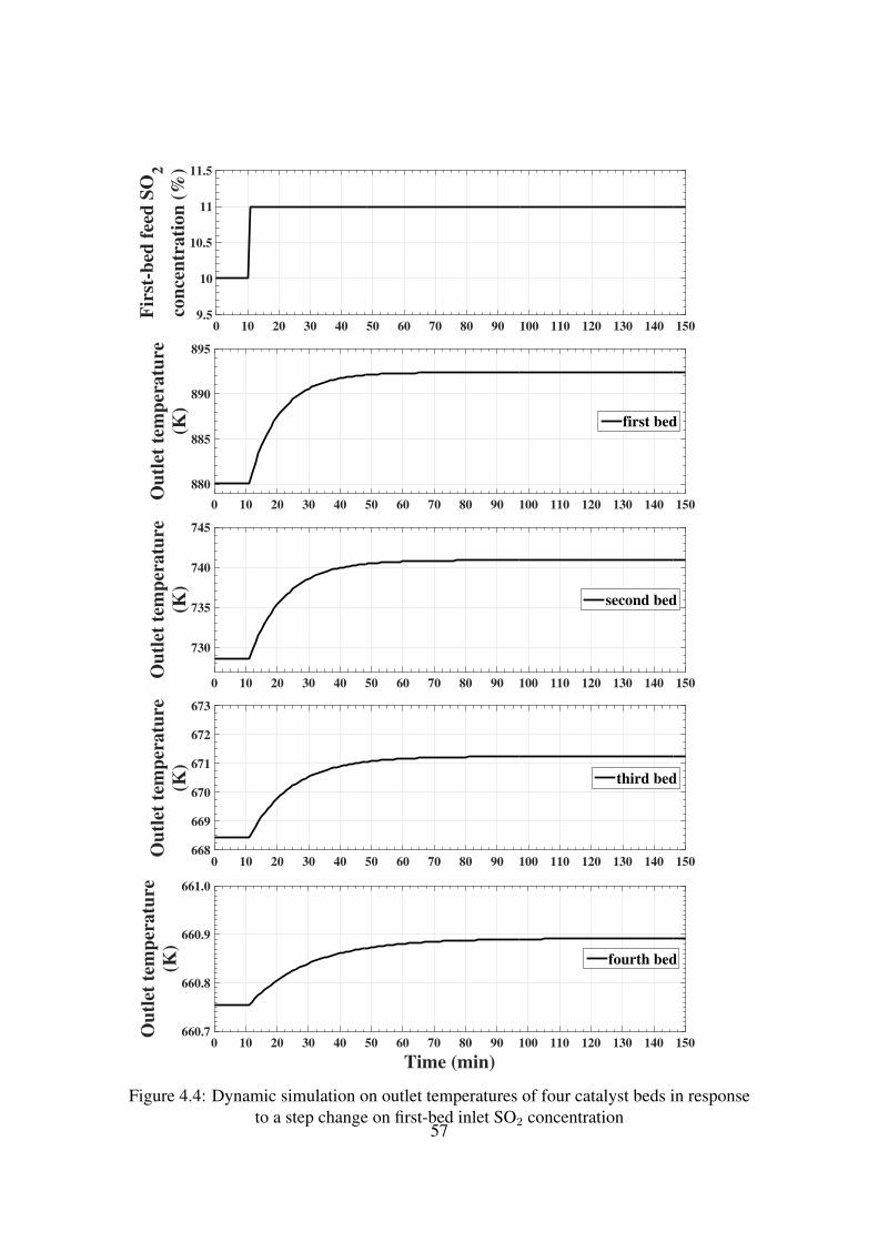
0 10 20 30 40 50 60 70 80 90 100 110 120 130 140 150

Fir

st-b

ed

feed

SO

2

co

ncen

tra

tio

n (

%)

9.5

10

10.5

11

11.5

0 10 20 30 40 50 60 70 80 90 100 110 120 130 140 150

Ou

tlet

tem

per

atu

re

(K)

880

885

890

895

first bed

0 10 20 30 40 50 60 70 80 90 100 110 120 130 140 150

Ou

tlet

tem

per

atu

re

(K)

730

735

740

745

second bed

0 10 20 30 40 50 60 70 80 90 100 110 120 130 140 150

Ou

tlet

tem

per

atu

re

(K)

668

669

670

671

672

673

third bed

Time (min)0 10 20 30 40 50 60 70 80 90 100 110 120 130 140 150

Ou

tlet

tem

per

atu

re

(K)

660.7

660.8

660.9

661.0

fourth bed

Figure 4.4: Dynamic simulation on outlet temperatures of four catalyst beds in responseto a step change on first-bed inlet SO2 concentration

57

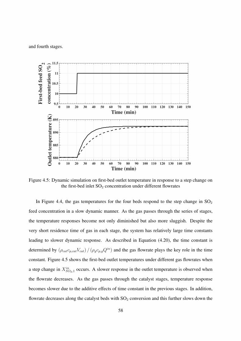
and fourth stages.

Time (min)0 10 20 30 40 50 60 70 80 90 100 110 120 130 140 150

Fir

st-b

ed f

eed

SO

2

con

cen

trati

on

(%

)

9.5

10

10.5

11

11.5

Time (min)0 10 20 30 40 50 60 70 80 90 100 110 120 130 140 150O

utl

et t

emp

eratu

re (

K)

880

885

890

895

Figure 4.5: Dynamic simulation on first-bed outlet temperature in response to a step change onthe first-bed inlet SO2 concentration under different flowrates

In Figure 4.4, the gas temperatures for the four beds respond to the step change in SO2

feed concentration in a slow dynamic manner. As the gas passes through the series of stages,

the temperature responses become not only diminished but also more sluggish. Despite the

very short residence time of gas in each stage, the system has relatively large time constants

leading to slower dynamic response. As described in Equation (4.20), the time constant is

determined by (ρcatcp,catVcat) / (ρgcp,gQin) and the gas flowrate plays the key role in the time

constant. Figure 4.5 shows the first-bed outlet temperatures under different gas flowrates when

a step change in X inSO2,1

occurs. A slower response in the outlet temperature is observed when

the flowrate decreases. As the gas passes through the catalyst stages, temperature response

becomes slower due to the additive effects of time constant in the previous stages. In addition,

flowrate decreases along the catalyst beds with SO2 conversion and this further slows down the

58

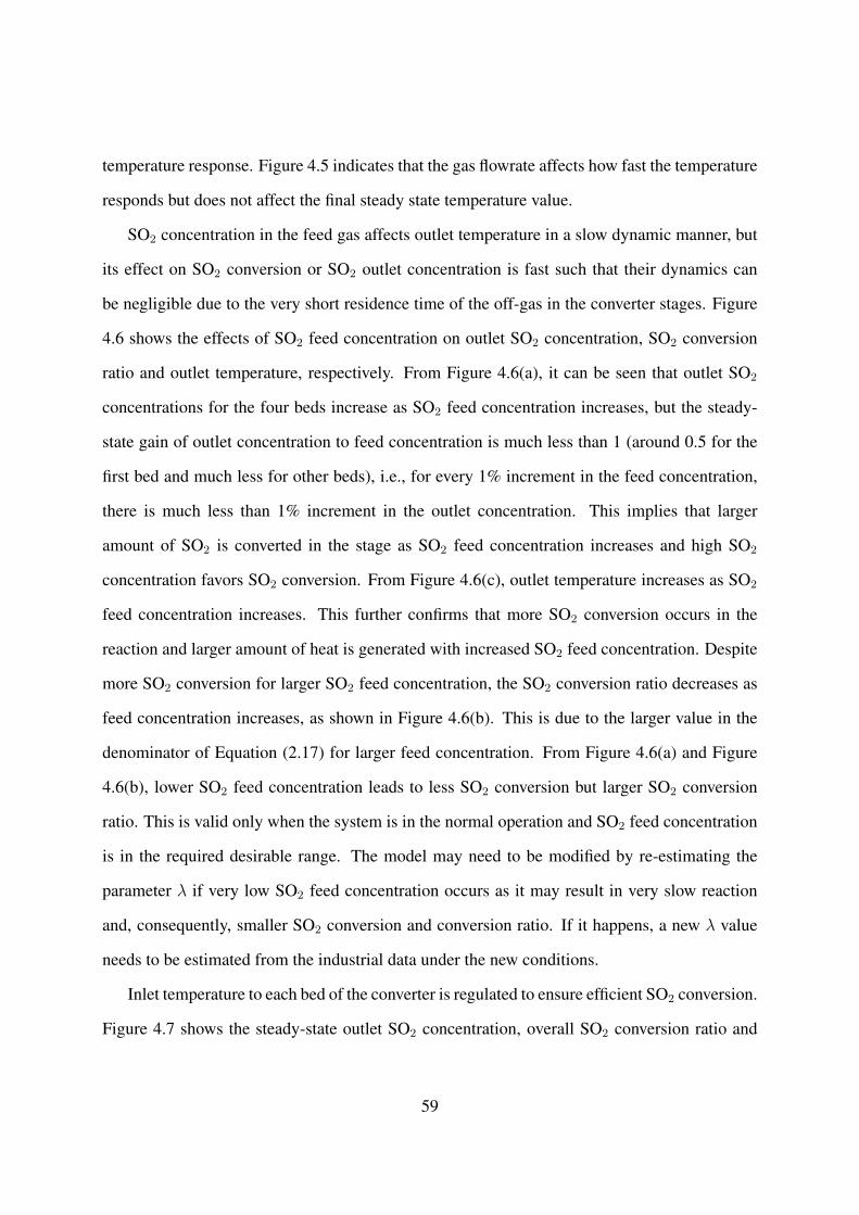
temperature response. Figure 4.5 indicates that the gas flowrate affects how fast the temperature

responds but does not affect the final steady state temperature value.

SO2 concentration in the feed gas affects outlet temperature in a slow dynamic manner, but

its effect on SO2 conversion or SO2 outlet concentration is fast such that their dynamics can

be negligible due to the very short residence time of the off-gas in the converter stages. Figure

4.6 shows the effects of SO2 feed concentration on outlet SO2 concentration, SO2 conversion

ratio and outlet temperature, respectively. From Figure 4.6(a), it can be seen that outlet SO2

concentrations for the four beds increase as SO2 feed concentration increases, but the steady-

state gain of outlet concentration to feed concentration is much less than 1 (around 0.5 for the

first bed and much less for other beds), i.e., for every 1% increment in the feed concentration,

there is much less than 1% increment in the outlet concentration. This implies that larger

amount of SO2 is converted in the stage as SO2 feed concentration increases and high SO2

concentration favors SO2 conversion. From Figure 4.6(c), outlet temperature increases as SO2

feed concentration increases. This further confirms that more SO2 conversion occurs in the

reaction and larger amount of heat is generated with increased SO2 feed concentration. Despite

more SO2 conversion for larger SO2 feed concentration, the SO2 conversion ratio decreases as

feed concentration increases, as shown in Figure 4.6(b). This is due to the larger value in the

denominator of Equation (2.17) for larger feed concentration. From Figure 4.6(a) and Figure

4.6(b), lower SO2 feed concentration leads to less SO2 conversion but larger SO2 conversion

ratio. This is valid only when the system is in the normal operation and SO2 feed concentration

is in the required desirable range. The model may need to be modified by re-estimating the

parameter λ if very low SO2 feed concentration occurs as it may result in very slow reaction

and, consequently, smaller SO2 conversion and conversion ratio. If it happens, a new λ value

needs to be estimated from the industrial data under the new conditions.

Inlet temperature to each bed of the converter is regulated to ensure efficient SO2 conversion.

Figure 4.7 shows the steady-state outlet SO2 concentration, overall SO2 conversion ratio and

59

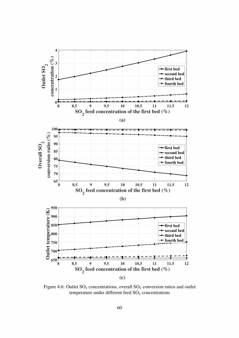
SO2 feed concentration of the first bed (%)

(a)

8 8.5 9 9.5 10 10.5 11 11.5 12

Ou

tlet

SO

2

con

cen

trati

on

(%

)

0

1

2

3

4

first bed

second bed

third bed

fourth bed


(b)

8 8.5 9 9.5 10 10.5 11 11.5 12

Overall

SO

2

con

versi

on

rati

o (

%)

65

70

75

80

85

90

95

100

first bed

second bed

third bed

fourth bed


(c)

8 8.5 9 9.5 10 10.5 11 11.5 12

Ou

tlet

tem

per

atu

re (

K)

650

700

750

800

850

900

950

first bed

second bed

third bed

fourth bed

Figure 4.6: Outlet SO2 concentrations, overall SO2 conversion ratios and outlettemperature under different feed SO2 concentrations

60

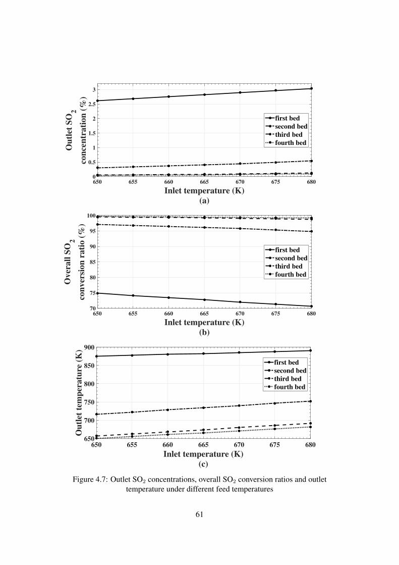
Inlet temperature (K)

(a)

650 655 660 665 670 675 680

Ou

tlet

SO

2

con

cen

trati

on

(%

)

0

0.5

1

1.5

2

2.5

3

first bed

second bed

third bed

fourth bed


(b)

650 655 660 665 670 675 680

Over

all

SO

2

con

ver

sion

rati

o (

%)

70

75

80

85

90

95

100

first bed

second bed

third bed

fourth bed


(c)

650 655 660 665 670 675 680

Ou

tlet

tem

per

atu

re (

K)

650

700

750

800

850

900

first bed

second bed

third bed

fourth bed

Figure 4.7: Outlet SO2 concentrations, overall SO2 conversion ratios and outlettemperature under different feed temperatures

61

Inlet O2 to SO

2 concentration ratio

(a)

0.6 0.7 0.8 0.9 1 1.1 1.2 1.3 1.4 1.5

Ou

tlet

SO

2

con

cen

trati

on

(%

)

0

0.5

1

1.5

2

2.5

3

3.5

first bed

second bed

third bed

fourth bed

Inlet O2 to SO


(b)

0.6 0.7 0.8 0.9 1 1.1 1.2 1.3 1.4 1.5

Overall

SO

2

con

versi

on

rati

o (

%)

65

70

75

80

85

90

95

100

first bed

second bed

third bed

fourth bed

Inlet O2 to SO


(c)

0.6 0.7 0.8 0.9 1 1.1 1.2 1.3 1.4 1.5

Ou

tlet

tem

per

atu

re (

K)

650

700

750

800

850

900

first bed

second bed

third bed

fourth bed

Figure 4.8: Outlet SO2 concentrations, overall SO2 conversion ratios and outlettemperature under different inlet O2 to SO2 concentration ratios

62

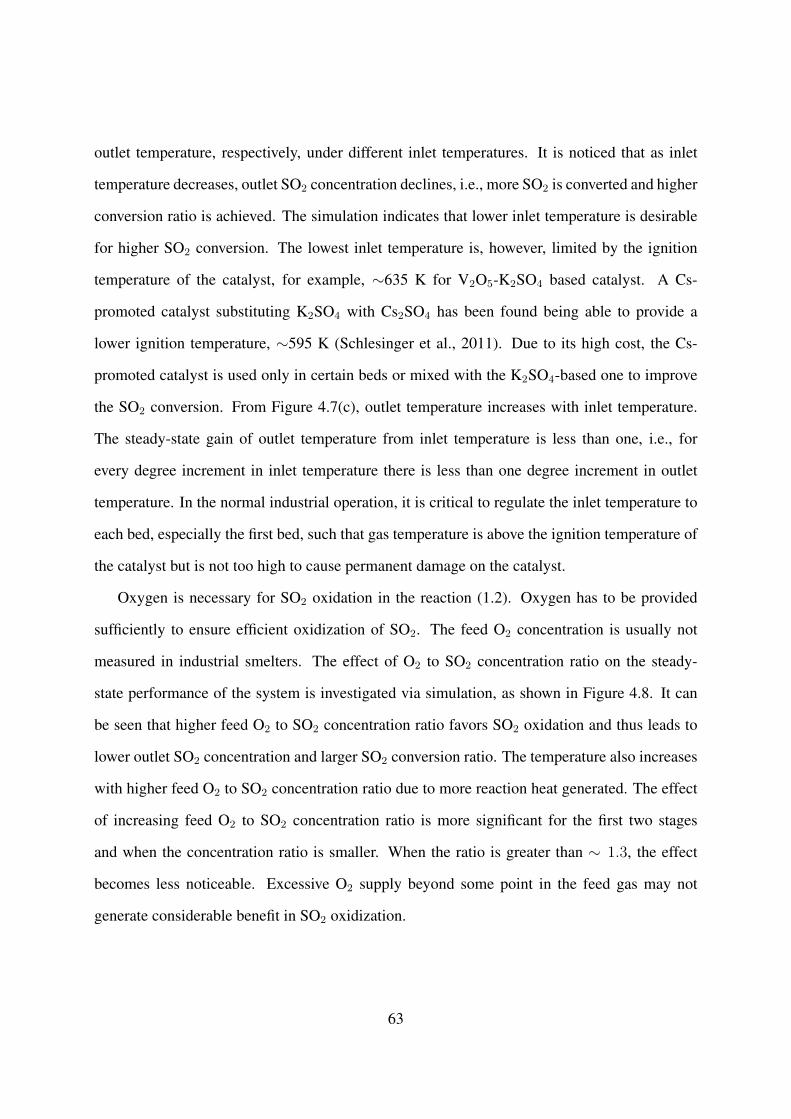
outlet temperature, respectively, under different inlet temperatures. It is noticed that as inlet

temperature decreases, outlet SO2 concentration declines, i.e., more SO2 is converted and higher

conversion ratio is achieved. The simulation indicates that lower inlet temperature is desirable

for higher SO2 conversion. The lowest inlet temperature is, however, limited by the ignition

temperature of the catalyst, for example, ∼635 K for V2O5-K2SO4 based catalyst. A Cs-

promoted catalyst substituting K2SO4 with Cs2SO4 has been found being able to provide a

lower ignition temperature, ∼595 K (Schlesinger et al., 2011). Due to its high cost, the Cs-

promoted catalyst is used only in certain beds or mixed with the K2SO4-based one to improve

the SO2 conversion. From Figure 4.7(c), outlet temperature increases with inlet temperature.

The steady-state gain of outlet temperature from inlet temperature is less than one, i.e., for

every degree increment in inlet temperature there is less than one degree increment in outlet

temperature. In the normal industrial operation, it is critical to regulate the inlet temperature to

each bed, especially the first bed, such that gas temperature is above the ignition temperature of

the catalyst but is not too high to cause permanent damage on the catalyst.

Oxygen is necessary for SO2 oxidation in the reaction (1.2). Oxygen has to be provided

sufficiently to ensure efficient oxidization of SO2. The feed O2 concentration is usually not

measured in industrial smelters. The effect of O2 to SO2 concentration ratio on the steady-

state performance of the system is investigated via simulation, as shown in Figure 4.8. It can

be seen that higher feed O2 to SO2 concentration ratio favors SO2 oxidation and thus leads to

lower outlet SO2 concentration and larger SO2 conversion ratio. The temperature also increases

with higher feed O2 to SO2 concentration ratio due to more reaction heat generated. The effect

of increasing feed O2 to SO2 concentration ratio is more significant for the first two stages

and when the concentration ratio is smaller. When the ratio is greater than ∼ 1.3, the effect

becomes less noticeable. Excessive O2 supply beyond some point in the feed gas may not

generate considerable benefit in SO2 oxidization.

63

4.6 Summary

In this chapter, a dynamic model of the catalytic SO2 converter in an industrial smelter is

developed based on mass and energy conservations. The developed model uses the SO2

conversion ratios as a key variable, which has high industrial relevance in the smelters. In

contrast to the existing models, the proposed model in this paper does not require reaction

kinetics knowledge or kinetics parameters and thus can be useful when accurate kinetics

information is not available. Comparison of model predicted temperature with the industrial

operating data indicates that the derived model is valid in describing the industrial system.

Based on the developed model, simulations are performed to investigate the process

dynamics and effects of process input variables. Results indicate that gas temperature out of the

converter stages has slow dynamics and gas flowrate is the key variable affecting the dynamics.

Examinations on the steady-state effect of input variables show that more SO2 conversion

occurs with higher SO2 feed concentration but SO2 conversion ratio decreases. When gas inlet

temperature is above the catalyst’s ignition point, SO2 conversion decreases with increasing

temperature.

The obtained model contains a parameter that is easy to be estimated from industrial

operating data and can thus be adapted to describe a variety of SO2 converters under different

operating conditions. The developed model provides a necessary foundation for process

optimization and enhanced control development for industrial smelters.

64

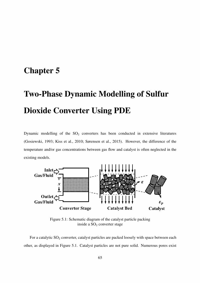
Chapter 5

Two-Phase Dynamic Modelling of Sulfur

Dioxide Converter Using PDE

Dynamic modelling of the SO2 converters has been conducted in extensive literatures

(Gosiewski, 1993; Kiss et al., 2010; Sørensen et al., 2015). However, the difference of the

temperature and/or gas concentrations between gas flow and catalyst is often neglected in the

existing models.

Figure 5.1: Schematic diagram of the catalyst particle packinginside a SO2 converter stage

For a catalytic SO2 converter, catalyst particles are packed loosely with space between each

other, as displayed in Figure 5.1. Catalyst particles are not pure solid. Numerous pores exist

65

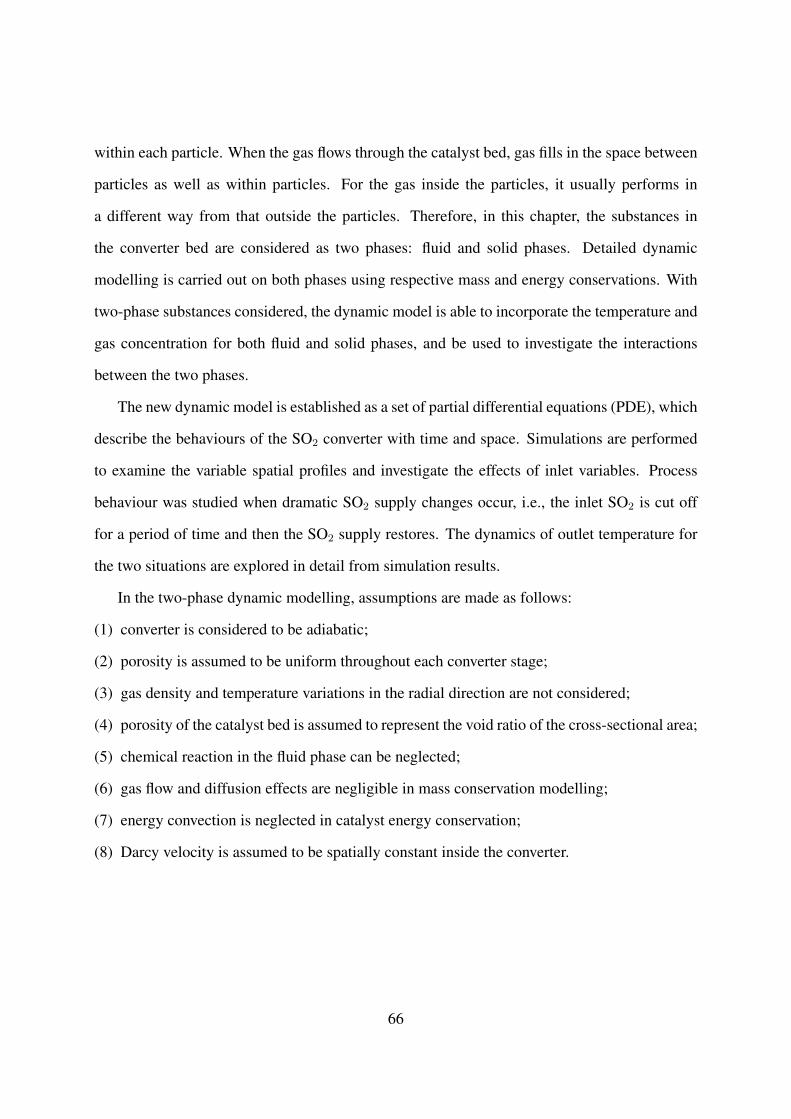
within each particle. When the gas flows through the catalyst bed, gas fills in the space between

particles as well as within particles. For the gas inside the particles, it usually performs in

a different way from that outside the particles. Therefore, in this chapter, the substances in

the converter bed are considered as two phases: fluid and solid phases. Detailed dynamic

modelling is carried out on both phases using respective mass and energy conservations. With

two-phase substances considered, the dynamic model is able to incorporate the temperature and

gas concentration for both fluid and solid phases, and be used to investigate the interactions

between the two phases.

The new dynamic model is established as a set of partial differential equations (PDE), which

describe the behaviours of the SO2 converter with time and space. Simulations are performed

to examine the variable spatial profiles and investigate the effects of inlet variables. Process

behaviour was studied when dramatic SO2 supply changes occur, i.e., the inlet SO2 is cut off

for a period of time and then the SO2 supply restores. The dynamics of outlet temperature for

the two situations are explored in detail from simulation results.

In the two-phase dynamic modelling, assumptions are made as follows:

(1) converter is considered to be adiabatic;

(2) porosity is assumed to be uniform throughout each converter stage;

(3) gas density and temperature variations in the radial direction are not considered;

(4) porosity of the catalyst bed is assumed to represent the void ratio of the cross-sectional area;

(5) chemical reaction in the fluid phase can be neglected;

(6) gas flow and diffusion effects are negligible in mass conservation modelling;

(7) energy convection is neglected in catalyst energy conservation;

(8) Darcy velocity is assumed to be spatially constant inside the converter.

66

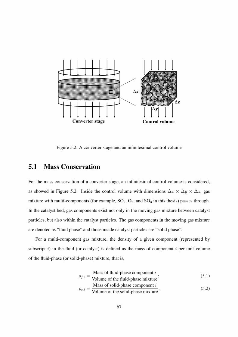
x

Converter stage Control volume

Figure 5.2: A converter stage and an infinitesimal control volume

5.1 Mass Conservation

For the mass conservation of a converter stage, an infinitesimal control volume is considered,

as showed in Figure 5.2. Inside the control volume with dimensions ∆x × ∆y × ∆z, gas

mixture with multi-components (for example, SO2, O2, and SO3 in this thesis) passes through.

In the catalyst bed, gas components exist not only in the moving gas mixture between catalyst

particles, but also within the catalyst particles. The gas components in the moving gas mixture

are denoted as “fluid phase” and those inside catalyst particles are “solid phase”.

For a multi-component gas mixture, the density of a given component (represented by

subscript i) in the fluid (or catalyst) is defined as the mass of component i per unit volume

of the fluid-phase (or solid-phase) mixture, that is,

ρf,i =Mass of fluid-phase component i

Volume of the fluid-phase mixture; (5.1)

ρs,i =Mass of solid-phase component i

Volume of the solid-phase mixture, (5.2)

67

and the total density of the fluid-phase (or solid-phase) mixture is the total mass of the fluid-

phase (or solid-phase) mixture in the fluid-phase (or solid-phase) volume:

ρf =Mass of fluid-phase mixture

Volume of the fluid-phase mixture=

∑i Mass of fluid-phase component i

Volume of the fluid-phase mixture

=∑i

ρf,i;(5.3)

ρs =Mass of solid-phase mixture

Volume of the solid-phase mixture=

∑i Mass of solid-phase component i

Volume of the solid-phase mixture

=∑i

ρs,i;(5.4)

Apart from density, mass concentration can be expressed by molar concentration as well.

For the fluid-phase component i, its molar concentration is defined as the number of moles of i

existing per unit volume of the fluid mixture. It is known that one mole of any components has

a mass equal to its molecular weight. Therefore, molar concentration of fluid-phase component

i, by definition, is:

Cf,i =Number of moles of fluid-phase component i


={Mass of fluid-phase component i}/{Molecular weight of i}


=ρf,iMi

, (5.5)

where M [g/mol] denotes the molecular weight. Solid-phase molar concentration is expressed

similarly as:

Cs,i =ρs,iMi

. (5.6)

68

5.1.1 Fluid-Phase Mass Conservation

In the control volume shown in Figure 5.2, when the fluid-phase is considered, the mass balance

of component i can be stated as follows:

[net rate of mass

accumulation of fluid-phase i in control volume

]=

[rate of mass

influx of fluid-phasei to control volume

]−[

rate of massefflux of fluid-phasei from control volume

]+

[rate of mass transferof i from solid phase

to fluid phase in control volume

]

+

[rate of chemical

production of fluid-phasei in control volume

].

(5.7)

If the total volume of the control volume is expressed as Vcv, which equals to (∆x∆y∆z),

the volumes of fluid-phase Vf and solid-phase Vs mixtures are:

Vcv = Vf + Vs, (5.8)

Vf = εVcv = ε∆x∆y∆z, (5.9)

Vs = (1− ε)Vcv = (1− ε)∆x∆y∆z, (5.10)

where ε denotes the porosity of the catalyst bed. For simplicity, the density and temperature

variations in the radial direction are not considered in this two-phase dynamic modelling, since

the radial dispersion becomes negligible during normal industrial operations (Mann et al., 1986;

Gosiewski, 1993). Therefore, both concentration and temperature gradients are taken into

account only in the gas flow direction x. If the porosity of the catalyst bed is assumed to

represent the void ratio of the cross-sectional area, the cross-sectional areas Scs of both phases

perpendicular to x in the control volume can be simply expressed as:

Scs,f =Vf∆x

= ε∆y∆z, (5.11)

Scs,s =Vs∆x

= (1− ε)∆y∆z. (5.12)

69

In Equation (5.7), the net rate of mass accumulation of fluid-phase i within the control

volume is given as:

[net rate of mass accumulation

of fluid-phase i in control volume]

=∆ρf,i∆t· Vf

= ε∆ρf,i∆t· (∆x∆y∆z) .

(5.13)

The rates of mass influx of i to the control volume and efflux from the control volume are:

[rate of mass influx of

fluid-phase i to control volume]

=(ρf,ivi|x

)· (ε∆y∆z) , (5.14)[

rate of mass efflux offluid-phase i from control volume

]=(ρf,ivi|x+∆x

)· (ε∆y∆z) , (5.15)

where vi stands for the absolute velocity of component i relative to stationary coordinate axes.

The mass flux of component i relative to the average velocity v of the fluid-phase gas mixture

is defined as mass diffusion ji (kg/(m2·sec)). According to an empirical relation postulated by

Fick (Fick, 1855), this mass flux takes the form as:

ji = −Di∇ρf,i, (5.16)

where Di [m2/sec] is the mass diffusivity or diffusion coefficient of component i through the

fluid mixture. Besides, the mass flux of component i to the average velocity can also be

expressed as (Lam, 2006; Welty et al., 2008):

ji = ρf,i (vi − v) . (5.17)

Equating Equations (5.16) and (5.17), it yields:

ρf,ivi = −Di∂ρf,i∂x

+ ρf,iv. (5.18)

70

The mass transfer between fluid- and solid-phase i takes place due to their mass

concentration difference. Written in a way analogous to Newton’s law of cooling (Welty et al.,

2008), the mass flux of i, j∗i [kg/(m2·sec)], caused by fluid-solid phase density difference has


j∗i = βi(ρs,i − ρf,i), (5.19)

where β [m/sec] is defined as the mass transfer coefficient. Actually, j∗i represents the mass

of component i passes through a unit contact area between fluid and catalyst particle per given

increment of time due to the density difference between fluid and solid phases. When solid-

phase density of i is higher than the fluid-phase one, j∗i is positive and transfer of component i

goes from solid phase to fluid phase. A negative j∗i represents that component i is transferring

from the fluid phase to solid phase. With Equation (5.19), rate of mass transfer of i from solid

phase in (5.7) is derived as:

[rate of mass transfer of i from

solid phase to fluid phase in control volume]

= j∗i ·SpVp· Vs, (5.20)

where Vp is the volume of one catalyst particle and Sp is the contact surface of fluid with one

catalyst particle. If a specific area ap [1/m] is introduced as:

ap =SpVp, (5.21)

Equation (5.20) becomes:


solid phase to fluid phase in control volume]

= j∗i · ap · Vs

= (1− ε)βiap(ρs,i − ρf,i) ·∆x∆y∆z.

(5.22)

For the concerned reaction (1.2), catalyst is necessary and essential, and thus the chemical

71

reaction in the fluid-phase can be neglected (Bousri et al., 2012):

[ rate of chemical production offluid-phase i in control volume

]= 0. (5.23)

When Equations (5.13-5.15), (5.22) and (5.23) are substituted into Equation (5.7), it yields:

∆ρf,i∆t· (ε∆x∆y∆z) =

(ρf,ivi|x

)· (ε∆y∆z)−

(ρf,ivi|x+∆x

)· (ε∆y∆z)

+ (1− ε)βiap(ρs,i − ρf,i) ·∆x∆y∆z.

(5.24)

Diving by (∆x∆y∆z), mass conservation of fluid-phase i becomes:

ε∆ρf,i∆t

= ερf,ivi|x − ρf,ivi|x+∆x

∆x+ (1− ε)βiap(ρs,i − ρf,i). (5.25)

Evaluated in the limit as ∆x and ∆t approach zero, it gives:

ε∂ρf,i∂t

= −ε∂(ρf,ivi)

∂x+ (1− ε)βiap(ρs,i − ρf,i). (5.26)

Substituting Equation (5.18) into (5.26), one has the fluid-phase mass conservation regarding

density written as:

ε∂ρf,i∂t

= −ε ∂∂x

(−Di

∂ρf,i∂x

+ ρf,iv

)+ (1− ε)βiap(ρs,i − ρf,i)

= εDi∂

∂x

(∂ρf,i∂x

)− εv∂(ρf,i)

∂x+ (1− ε)βiap(ρs,i − ρf,i).

(5.27)

Converting the fluid-phase mass balance in Equation (5.27) into the one in terms of molar

concentration by using Equations (5.5) and (5.6), we can have the corresponding molar

concentration expression:

ε∂Cf,i∂t

= εDi∂

∂x

(∂Cf,i∂x

)− εv∂(Cf,i)

∂x+ (1− ε)βiap(Cs,i − Cf,i). (5.28)

72

5.1.2 Solid-Phase Mass Conservation

For the mass conservation of solid-phase mixture inside catalyst particles, the gas flow and

diffusion effects are usually negligible in dynamic modelling (Shahamiri and Wierzba, 2011;

Bousri et al., 2012). Therefore, the general expression of mass balance of solid-phase

component i may be stated as:

[net rate of mass

accumulation of solid-phase i in control volume

]=

[rate of mass transferof i from fluid phase

to solid phase in control volume

]+

[rate of chemical

production of solid-phasei in control volume

].

(5.29)

Similarly as Equations (5.13), (5.22) and (5.23), three terms in Equation (5.29) can be expressed

respectively as:

[net rate of mass accumulation

of solid-phase i in control volume]

=∆ρs,i∆t· Vs

= (1− ε) ∆ρs,i∆t·∆x∆y∆z,

(5.30)


fluid phase to solid phase in control volume]

=(1− ε)βiap(ρf,i − ρs,i) ·∆x∆y∆z,

(5.31)

[ rate of chemical production ofsolid-phase i in control volume

]=Rs,i (ρcatVs)

=(1− ε)Rs,iρcat ·∆x∆y∆z.

(5.32)

Here Rs,i [kg/(kg-cat·sec)] is the chemical production rate of gas component i with the help of

one unit mass of catalyst.

73

Substituting Equations (5.30-5.32) into Equation (5.29), it gives:

(1− ε) ∆ρs,i∆t·∆x∆y∆z

=(1− ε)βiap(ρf,i − ρs,i) ·∆x∆y∆z + (1− ε)Rs,iρcat ·∆x∆y∆z.

(5.33)

Diving by (1− ε) ∆x∆y∆z and applying evaluation in the limit when ∆x, ∆y, ∆z and ∆t

approach zero, we have:∂ρs,i∂t

= βiap(ρf,i − ρs,i) +Rs,iρcat. (5.34)

Expressed by molar concentrations with Equations (5.5) and (5.6), the differential equation of

solid-phase mass balance regarding component i can be written as:

∂Cs,i∂t

= βiap(Cf,i − Cs,i) + rs,iρcat, (5.35)

where rs,i [mol/(kg-cat·sec)] is related to Rs,i via:

rs,i = Rs,i ·Mi. (5.36)

74

5.2 Energy Conservation

5.2.1 Fluid-Phase Energy Conservation

Considering the control volume in Figure 5.2, energy balance of the fluid-phase mixture can be

given as:

[net rate of energy

accumulation of fluid phasein control volume

]=

[rate of energy

influx of fluid phaseto control volume

]−

[rate of energy

efflux of fluid phasefrom control volume

]

+

[rate of heat transfer

from solid phase to fluidphase in control volume

]

+

[rate of chemical reaction

heat release to fluidphase in control volume

](5.37)

If fluid-phase temperature change is ∆Tf for a given time increment ∆t, the net rate of

energy accumulation of fluid phase in the control volume is expressed as:

[net rate of energy accumulationof fluid phase in control volume

]= ρfVfcp,f

∆Tf∆t

= ερfcp,f∆Tf∆t·∆x∆y∆z,

(5.38)

where cp,f [J/(kg·K)] is the heat capacity of the fluid-phase mixture.

When fluid-phase gas mixture is assumed to flow in only x direction, the energy influx

and efflux of fluid phase include the energy transfer due to fluid flow across the void part of

control surface ε∆y∆z and conduction effect in the fluid-phase gas. According the Fourier’s

law concerning heat conduction, the conductive heat flux qf [J/(m2·sec)] can be stated by the

temperature gradient as (Janna, 1999):

qf = −kf∂Tf∂x

, (5.39)

where kf [J/(m·K·sec)] is the thermal conductivity of fluid-phase mixture. Therefore, the rate

75

of energy influx of fluid phase minus the rate of energy efflux is obtained as follows:

[ rate of energy influx offluid phase to control volume

]−[ rate of energy efflux offluid phase from control volume

]= ρfcp,fv

(Tf |x − Tf |x+∆x

)· (ε∆y∆z)︸︷︷︸

energy transfer due to fluid flow

+(qf |x − qf |x+∆x

)· (ε∆y∆z)︸︷︷︸

conductive effect

=ρfcp,fv(Tf |x − Tf |x+∆x

)· (ε∆y∆z) +

[(−kf

∂Tf∂x

)∣∣∣∣x

−(−kf

∂Tf∂x

)∣∣∣∣x+∆x

]· (ε∆y∆z) .

(5.40)

Energy transfer between solid and fluid phases occurs due to the existence of temperature

difference. For fluid flowing through porous catalyst bed, the heat flux q∗f [J/(m2·sec)] is used

to represent the energy exchange through a unit contact area between fluid and catalyst particle

per given increment of time as a result of heat transfer. Based on Newton’s law of cooling, q∗f

takes the form as (Janna, 1999):

q∗f = h (Ts − Tf ) , (5.41)

where h [J/(m2·K·sec)] is the heat transfer coefficient. In this case, the heat transfer rate from

solid phase to fluid phase in control volume is derived as:

[rate of heat transfer from solid

phase to fluid phase in control volume]

= q∗f ·SpVp· Vs

= q∗f · ap · Vs

= (1− ε)hap (Ts − Tf ) ·∆x∆y∆z.

(5.42)

Since reaction (1.2) requires the presence of catalyst, the chemical reaction within the fluid

phase is not considered here, and then we have:

[rate of chemical reaction heat release

to fluid phase in control volume]

= 0. (5.43)

76

Substituting Equations (5.38), (5.40), (5.42) and (5.43) into (5.37), we obtain:

ερfcp,f∆Tf∆t·∆x∆y∆z = ρfcp,fv

(Tf |x − Tf |x+∆x

)· (ε∆y∆z)

+

[(−kf

∂Tf∂x

)∣∣∣∣x

−(−kf

∂Tf∂x

)∣∣∣∣x+∆x

]· (ε∆y∆z)

+ (1− ε)hap (Ts − Tf ) ·∆x∆y∆z.

(5.44)

If Equation (5.44) is divided by ∆x∆y∆z and evaluated when ∆x, ∆y, ∆z and ∆t approach

zero, it yields:

ερfcp,f∂Tf∂t

= εkf∂

∂x

(∂Tf∂x

)− ερfcp,fv

∂Tf∂x

+ (1− ε)hap (Ts − Tf ) . (5.45)

5.2.2 Solid-Phase Energy Conservation

The energy balance for the solid phase holds a similar expression to the fluid phase and is given

as:[net rate of energy

accumulation of solid phasein control volume

]=

[rate of energy

influx of solid phaseto control volume

]−

[rate of energy

efflux of solid phasefrom control volume

]

+

[rate of heat

transfer from fluid phase tosolid phase in control volume

]

+

[rate of chemical reaction

heat release to solidphase in control volume

].

(5.46)

77

For the terms in (5.46), they can be expressed as:

[net rate of energy accumulationof solid phase in control volume

]=ρcatVscp,cat ·

∆Ts∆t

=(1− ε)ρcatcp,cat∆Ts∆t·∆x∆y∆z,

(5.47)

[ rate of energy influx ofsolid phase to control volume

]−[ rate of energy efflux ofsolid phase from control volume

]=(qs|x − qs|x+∆x

)· (1− ε) ∆y∆z︸︷︷︸

conductive effect

= (1− ε)[(−kcat

∂Ts∂x

)∣∣∣∣x

−(−kcat

∂Ts∂x

)∣∣∣∣x+∆x

]·∆y∆z,

(5.48)

[rate of convective heat transfer from fluid

phase to solid phase in control volume]

=q∗s ·SpVp· Vs

=q∗s · ap · Vs

=(1− ε)hap (Tf − Ts) ·∆x∆y∆z,

(5.49)

[rate of chemical reaction heat release

to solid phase in control volume]

=rh · (ρcatVs)

=(1− ε)rhρcat ·∆x∆y∆z,

(5.50)

where rh (J/(kg-cat·sec)) denotes the energy release rate by the catalytic chemical reaction. Note

that Equation (5.48) excludes the energy flux by gas flow, because the average solid-phase gas

flow velocity is assumed zero.

78

Substituting Equations (5.47-5.50) into (5.46), it gives:

(1− ε)ρcatcp,cat∆Ts∆t·∆x∆y∆z

= (1− ε)[(−kcat

∂Ts∂x

)∣∣∣∣x

−(−kcat

∂Ts∂x

)∣∣∣∣x+∆x

]·∆y∆z

+(1− ε)hap (Tf − Ts) ·∆x∆y∆z

+(1− ε)rhρcat ·∆x∆y∆z.

(5.51)

After being divided by (1− ε) ∆x∆y∆z and evaluated in the limit when ∆x, ∆y, ∆z and ∆t

approach zero, a partial differential equation for solid-phase energy conservation is obtained:

ρcatcp,cat∂Ts∂t

= kcat∂

∂x

(∂Ts∂x

)+ hap (Tf − Ts) + rhρcat (5.52)

5.3 Two-Phase Dynamic Modelling

5.3.1 Two-Phase Model for SO2 Converter

Combining the differential relationship developed above, the overall two-phase dynamic model

for the SO2 converter is summarized as follows:

energy conservations:

ερfcp,f ·∂Tf∂t

= εkf∂

∂x

(∂Tf∂x

)− ερfcp,fv ·

∂Tf∂x

+ (1− ε)hap (Ts − Tf ) , (5.53)

ρcatcp,cat ·∂Ts∂t

= kcat∂

∂x

(∂Ts∂x

)+ hap (Tf − Ts) + rhρcat, (5.54)

79

fluid-phase mass conservations:

ε∂Cf,SO2

∂t=εDSO2

∂

∂x

(∂Cf,SO2

∂x

)− εv · ∂Cf,SO2

∂x

+ (1− ε)βSO2ap(Cs,SO2 − Cf,SO2),

(5.55)

ε∂Cf,O2

∂t=εDO2

∂

∂x

(∂Cf,O2

∂x

)− εv · ∂Cf,O2

∂x

+ (1− ε)βO2ap(Cs,O2 − Cf,O2),

(5.56)

ε∂Cf,SO3

∂t=εDSO3

∂

∂x

(∂Cf,SO3

∂x

)− εv · ∂Cf,SO3

∂x

+ (1− ε)βSO3ap(Cs,SO3 − Cf,SO3),

(5.57)

solid-phase mass conservations:

∂Cs,SO2

∂t= βSO2ap(Cf,SO2 − Cs,SO2) + rs,SO2ρcat, (5.58)

∂Cs,O2

∂t= βO2ap(Cf,O2 − Cs,O2) + rs,O2ρcat, (5.59)

∂Cs,SO3

∂t= βSO3ap(Cf,SO3 − Cs,SO3) + rs,SO3ρcat. (5.60)

and the following boundary conditions will be applied at the inlet and outlet in our simulations:

at the inlet x = 0:

Tf (t, x = 0) = T in(t), (5.61)

Ts(t, x = 0) = T in(t), (5.62)

Cf,i(t, x = 0) = Cini (t) (5.63)

80

at the outlet x = xmax:

∂Tf∂x

∣∣∣∣x=xmax

= 0, (5.64)

∂Ts∂x

∣∣∣∣x=xmax

= 0, (5.65)

∂Cf,i∂x

∣∣∣∣x=xmax

= 0, (5.66)

∂Cs,i∂x

∣∣∣∣x=xmax

= 0, (5.67)

where i represents different gas components, SO2, O2 and SO3.

Average Fluid Velocity

With the first-bed inlet volume flowrateQin measured and collected from the smelter, the Darcy

velocity u can be calculated as:

u =Qin

π (DC/2)2 , (5.68)

where DC [m] is the diameter of the catalytic converter. The average fluid velocity v relates

with the Darcy velocity u by the porosity as:

v =u

ε. (5.69)

Spatial Pressure

Darcy’s law describes the relation between gas pressure gradient and flowrate (Darcy, 1856;

Holst and Aziz, 1972; Amhalhel and Furmanski, 1997):

u = − κ

µf

∂P

∂x, (5.70)

81

where κ [m2] represents Darcy permeability and µf [Pa·sec] is the fluid viscosity. If the Darcy

velocity u is assumed spatially constant in the converter, then pressure inside the converter stage

can be given as:

P (x) = P (0)− u κµfx. (5.71)

Equation (5.71) suggests that gas pressure decreases when gas flows along the x-direction.

5.3.2 Properties and Parameters

In the derived dynamic model from Equations (5.53) to (5.60) and (5.71), several parameters

are included and they should be determined for the next calculations.

Darcy Permeability

If the catalyst particles are considered to be spherical, Darcy permeability has the expression as

follows (Richardson et al., 2013):

κ = 0.0055ε3dp

(1− ε)2, [m2] (5.72)

where dp [m] is the catalyst particle diameter.

Viscosity

For fluid viscosity, its values of different gas components can be calculated by the following

empirical equation (Liessmann et al., 1995; Coker, 2007):

µ = Aµ +BµT + CµT2, [Pa·sec] (5.73)

82

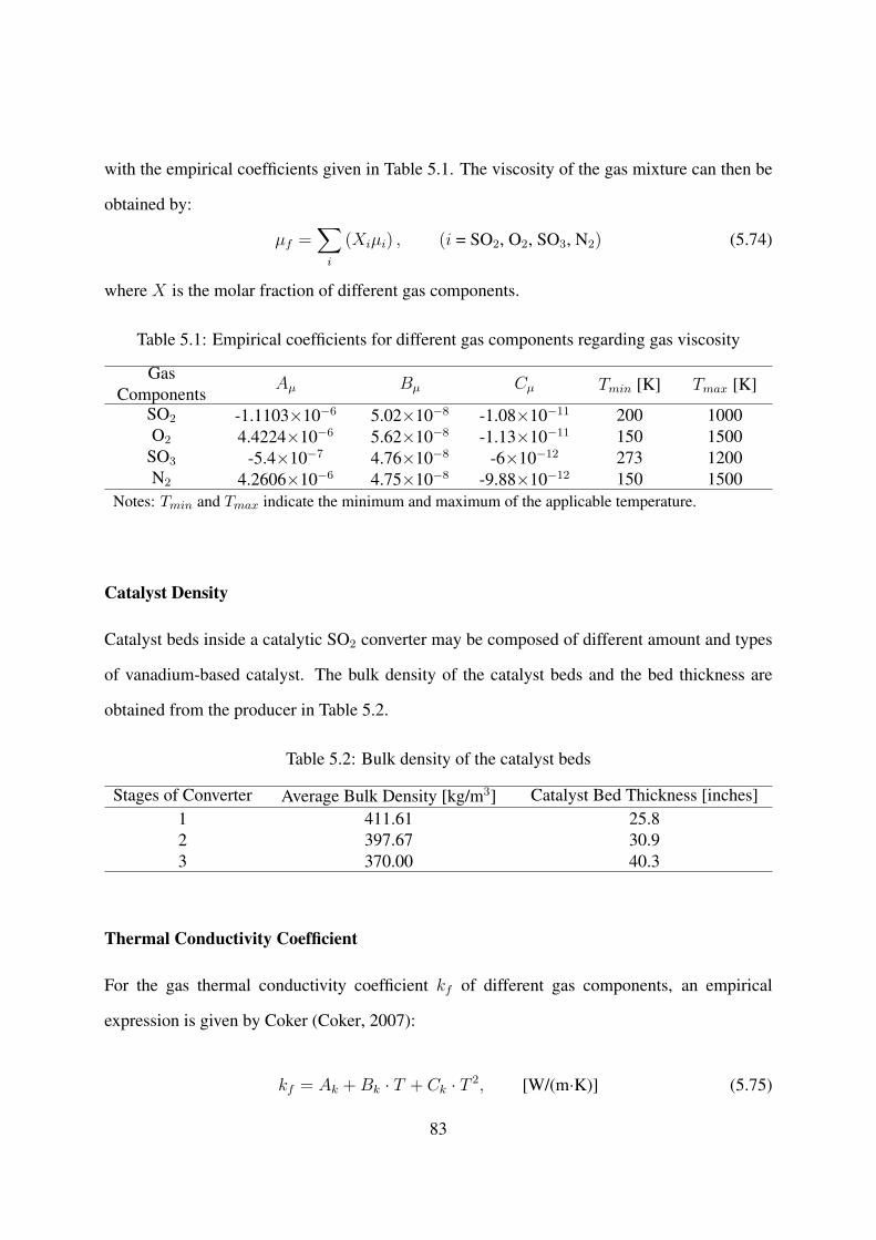
with the empirical coefficients given in Table 5.1. The viscosity of the gas mixture can then be

obtained by:

µf =∑i

(Xiµi) , (i = SO2, O2, SO3, N2) (5.74)

where X is the molar fraction of different gas components.

Table 5.1: Empirical coefficients for different gas components regarding gas viscosity

GasComponents

Aµ Bµ Cµ Tmin [K] Tmax [K]

SO2 -1.1103×10−6 5.02×10−8 -1.08×10−11 200 1000O2 4.4224×10−6 5.62×10−8 -1.13×10−11 150 1500

SO3 -5.4×10−7 4.76×10−8 -6×10−12 273 1200N2 4.2606×10−6 4.75×10−8 -9.88×10−12 150 1500

Notes: Tmin and Tmax indicate the minimum and maximum of the applicable temperature.

Catalyst Density

Catalyst beds inside a catalytic SO2 converter may be composed of different amount and types

of vanadium-based catalyst. The bulk density of the catalyst beds and the bed thickness are

obtained from the producer in Table 5.2.

Table 5.2: Bulk density of the catalyst beds

Stages of Converter Average Bulk Density [kg/m3] Catalyst Bed Thickness [inches]1 411.61 25.82 397.67 30.93 370.00 40.3

Thermal Conductivity Coefficient

For the gas thermal conductivity coefficient kf of different gas components, an empirical

expression is given by Coker (Coker, 2007):

kf = Ak +Bk · T + Ck · T 2, [W/(m·K)] (5.75)

83

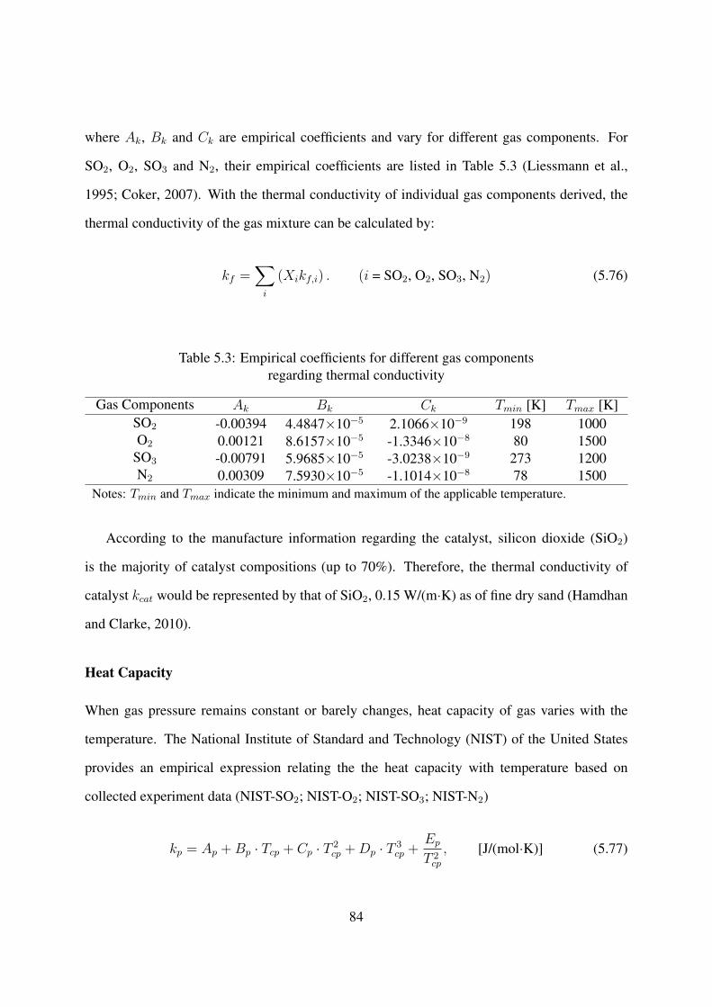
where Ak, Bk and Ck are empirical coefficients and vary for different gas components. For

SO2, O2, SO3 and N2, their empirical coefficients are listed in Table 5.3 (Liessmann et al.,

1995; Coker, 2007). With the thermal conductivity of individual gas components derived, the

thermal conductivity of the gas mixture can be calculated by:

kf =∑i

(Xikf,i) . (i = SO2, O2, SO3, N2) (5.76)

Table 5.3: Empirical coefficients for different gas componentsregarding thermal conductivity

Gas Components Ak Bk Ck Tmin [K] Tmax [K]SO2 -0.00394 4.4847×10−5 2.1066×10−9 198 1000O2 0.00121 8.6157×10−5 -1.3346×10−8 80 1500

SO3 -0.00791 5.9685×10−5 -3.0238×10−9 273 1200N2 0.00309 7.5930×10−5 -1.1014×10−8 78 1500


According to the manufacture information regarding the catalyst, silicon dioxide (SiO2)

is the majority of catalyst compositions (up to 70%). Therefore, the thermal conductivity of

catalyst kcat would be represented by that of SiO2, 0.15 W/(m·K) as of fine dry sand (Hamdhan

and Clarke, 2010).

Heat Capacity

When gas pressure remains constant or barely changes, heat capacity of gas varies with the

temperature. The National Institute of Standard and Technology (NIST) of the United States

provides an empirical expression relating the the heat capacity with temperature based on

collected experiment data (NIST-SO2; NIST-O2; NIST-SO3; NIST-N2)

kp = Ap +Bp · Tcp + Cp · T 2cp +Dp · T 3

cp +EpT 2cp

, [J/(mol·K)] (5.77)

84

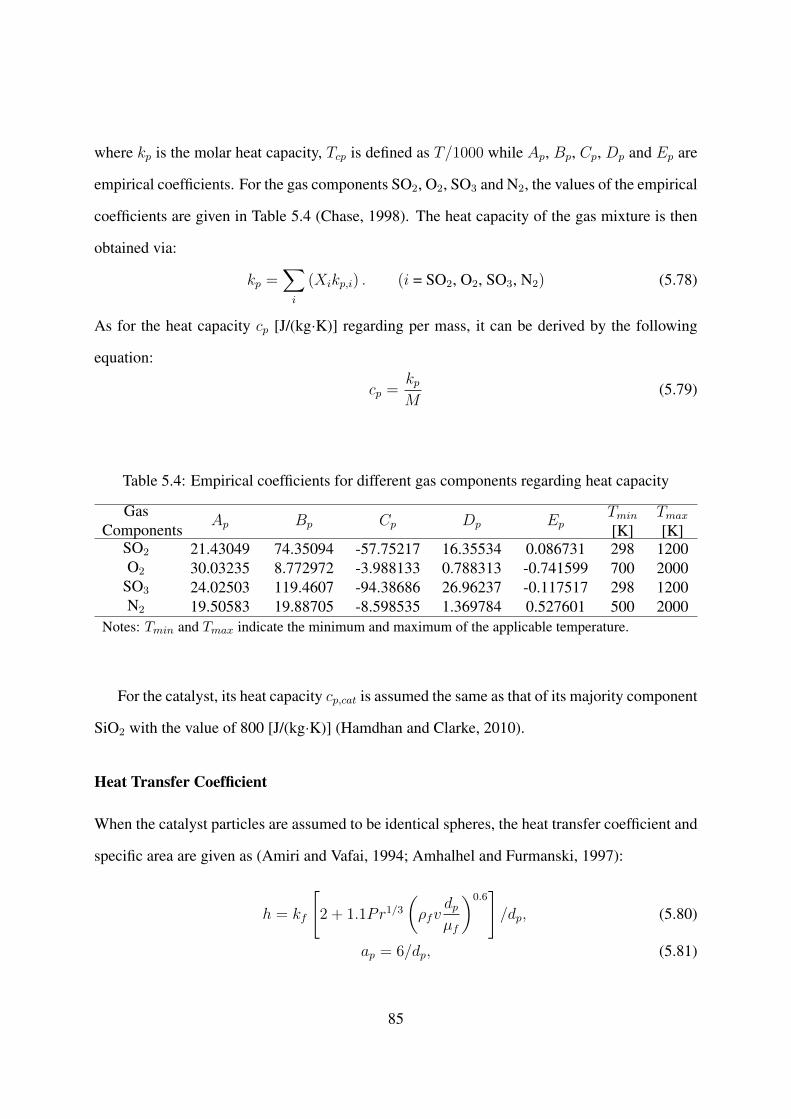
where kp is the molar heat capacity, Tcp is defined as T/1000 while Ap, Bp, Cp, Dp and Ep are

empirical coefficients. For the gas components SO2, O2, SO3 and N2, the values of the empirical

coefficients are given in Table 5.4 (Chase, 1998). The heat capacity of the gas mixture is then

obtained via:

kp =∑i

(Xikp,i) . (i = SO2, O2, SO3, N2) (5.78)

As for the heat capacity cp [J/(kg·K)] regarding per mass, it can be derived by the following

equation:

cp =kpM

(5.79)

Table 5.4: Empirical coefficients for different gas components regarding heat capacity

GasComponents

Ap Bp Cp Dp EpTmin[K]

Tmax[K]

SO2 21.43049 74.35094 -57.75217 16.35534 0.086731 298 1200O2 30.03235 8.772972 -3.988133 0.788313 -0.741599 700 2000

SO3 24.02503 119.4607 -94.38686 26.96237 -0.117517 298 1200N2 19.50583 19.88705 -8.598535 1.369784 0.527601 500 2000


For the catalyst, its heat capacity cp,cat is assumed the same as that of its majority component

SiO2 with the value of 800 [J/(kg·K)] (Hamdhan and Clarke, 2010).

Heat Transfer Coefficient

When the catalyst particles are assumed to be identical spheres, the heat transfer coefficient and

specific area are given as (Amiri and Vafai, 1994; Amhalhel and Furmanski, 1997):

h = kf

[2 + 1.1Pr1/3

(ρfv

dpµf

)0.6]/dp, (5.80)

ap = 6/dp, (5.81)

85

where dp [m] represents the particle diameter, µf denotes the viscosity of the fluid mixture and

Pr is the Prandtl number with the following expression:

Pr =µfcp,fkf

. (5.82)

Diffusion Coefficient

For a binary gas mixture with components a and b, diffusion coefficient has an expression given

below (Thirumaleshwar, 2009):

Dab = 0.0043 · T 3/2

Pt

(V

1/3m,a + V

1/3m,b

)2 ·(

1

Ma

+1

Mb

)1/2

, [cm2/sec] (5.83)

where Vm,a and Vm,b are molar volumes of components a and b at normal boiling points,

respectively, with a unit of [cm3/mol]. If fluid-phase gas mixture is assumed to be air, the

diffusion coefficients of SO2, O2, SO3 and N2 can be derived with the given molar weight and

molar volume in Table 5.5 (Thirumaleshwar, 2009).

Table 5.5: Molar weights and molar volumes for different gas components

Gas Components Molecular Weight [g/mol] Molar Volumes [cm3/mol]Air 29 29.89SO2 64 44.78O2 32 25.63

SO3 48 20.10N2 28 31.20

86

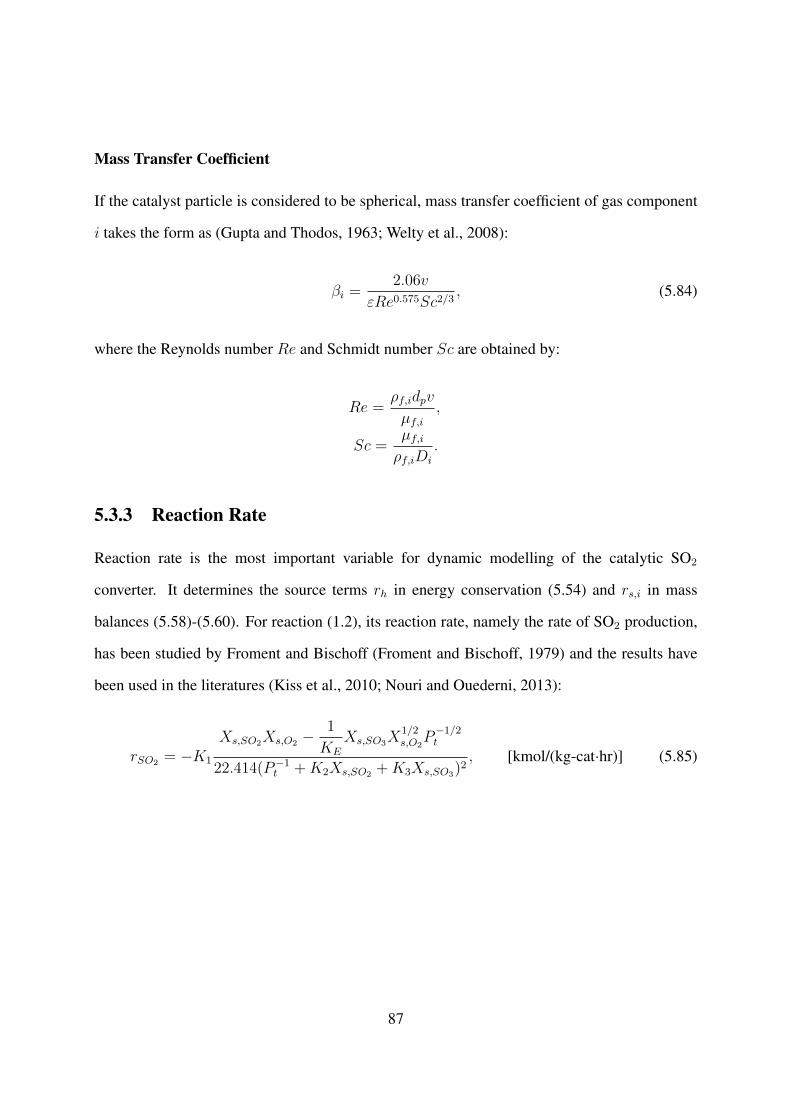
Mass Transfer Coefficient

If the catalyst particle is considered to be spherical, mass transfer coefficient of gas component

i takes the form as (Gupta and Thodos, 1963; Welty et al., 2008):

βi =2.06v

εRe0.575Sc2/3, (5.84)

where the Reynolds number Re and Schmidt number Sc are obtained by:

Re =ρf,idpv

µf,i,

Sc =µf,iρf,iDi

.

5.3.3 Reaction Rate

Reaction rate is the most important variable for dynamic modelling of the catalytic SO2

converter. It determines the source terms rh in energy conservation (5.54) and rs,i in mass

balances (5.58)-(5.60). For reaction (1.2), its reaction rate, namely the rate of SO2 production,

has been studied by Froment and Bischoff (Froment and Bischoff, 1979) and the results have

been used in the literatures (Kiss et al., 2010; Nouri and Ouederni, 2013):

rSO2 = −K1

Xs,SO2Xs,O2 −1

KE

Xs,SO3X1/2s,O2

P−1/2t

22.414(P−1t +K2Xs,SO2 +K3Xs,SO3)

2, [kmol/(kg-cat·hr)] (5.85)

87

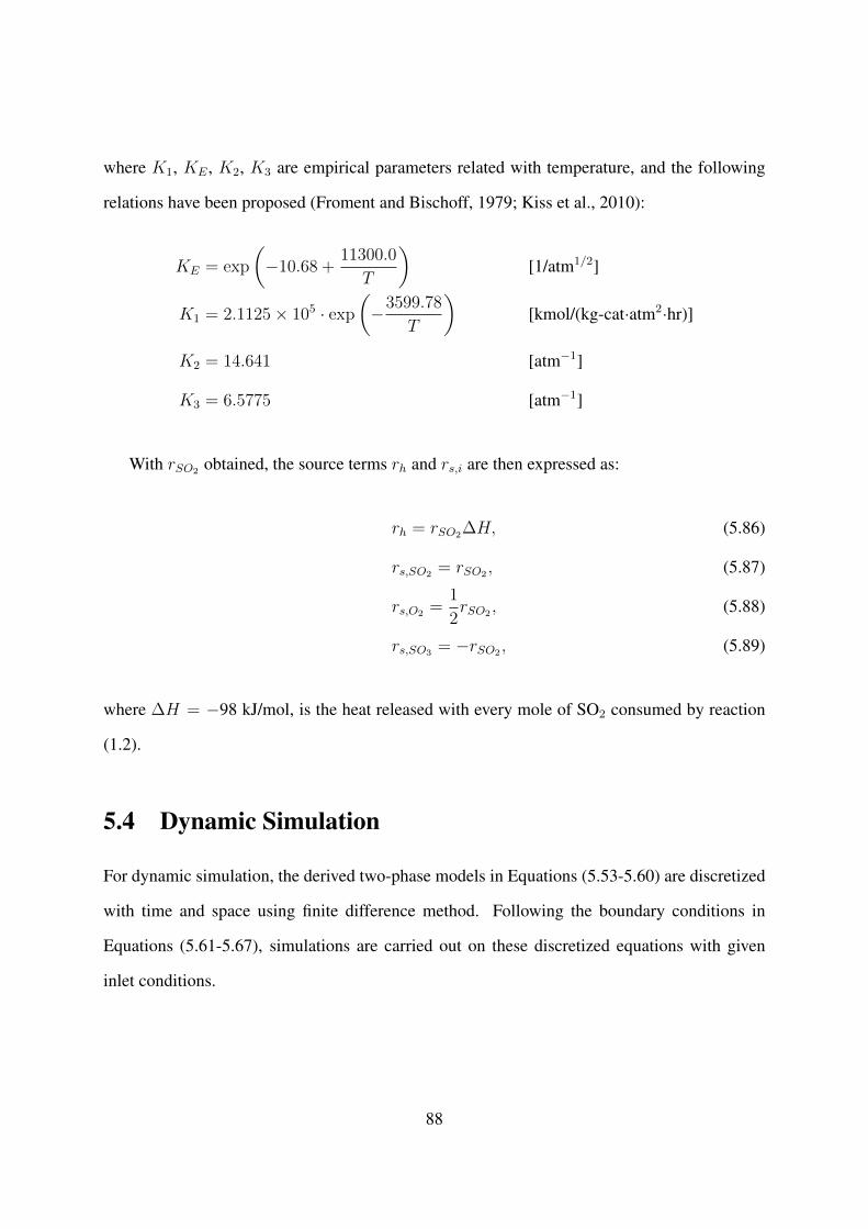
where K1, KE , K2, K3 are empirical parameters related with temperature, and the following

relations have been proposed (Froment and Bischoff, 1979; Kiss et al., 2010):

KE = exp

(−10.68 +

11300.0

T

)[1/atm1/2]

K1 = 2.1125× 105 · exp

(−3599.78

T

)[kmol/(kg-cat·atm2·hr)]

K2 = 14.641 [atm−1]

K3 = 6.5775 [atm−1]

With rSO2 obtained, the source terms rh and rs,i are then expressed as:

rh = rSO2∆H, (5.86)

rs,SO2 = rSO2 , (5.87)

rs,O2 =1

2rSO2 , (5.88)

rs,SO3 = −rSO2 , (5.89)

where ∆H = −98 kJ/mol, is the heat released with every mole of SO2 consumed by reaction

(1.2).

5.4 Dynamic Simulation

For dynamic simulation, the derived two-phase models in Equations (5.53-5.60) are discretized

with time and space using finite difference method. Following the boundary conditions in

Equations (5.61-5.67), simulations are carried out on these discretized equations with given

inlet conditions.

88

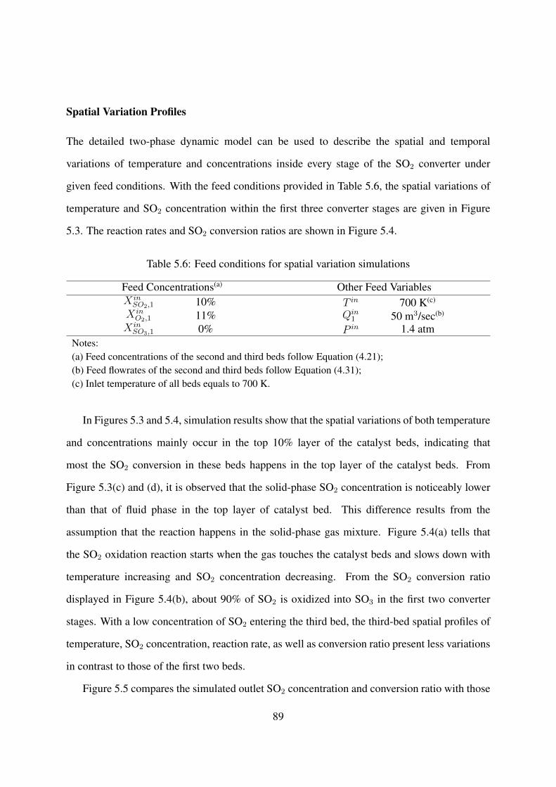
Spatial Variation Profiles

The detailed two-phase dynamic model can be used to describe the spatial and temporal

variations of temperature and concentrations inside every stage of the SO2 converter under

given feed conditions. With the feed conditions provided in Table 5.6, the spatial variations of

temperature and SO2 concentration within the first three converter stages are given in Figure

5.3. The reaction rates and SO2 conversion ratios are shown in Figure 5.4.

Table 5.6: Feed conditions for spatial variation simulations

Feed Concentrations(a) Other Feed VariablesX inSO2,1 10% T in 700 K(c)

X inO2,1 11% Qin

1 50 m3/sec(b)

X inSO3,1 0% P in 1.4 atm

Notes:(a) Feed concentrations of the second and third beds follow Equation (4.21);(b) Feed flowrates of the second and third beds follow Equation (4.31);(c) Inlet temperature of all beds equals to 700 K.

In Figures 5.3 and 5.4, simulation results show that the spatial variations of both temperature

and concentrations mainly occur in the top 10% layer of the catalyst beds, indicating that

most the SO2 conversion in these beds happens in the top layer of the catalyst beds. From

Figure 5.3(c) and (d), it is observed that the solid-phase SO2 concentration is noticeably lower

than that of fluid phase in the top layer of catalyst bed. This difference results from the

assumption that the reaction happens in the solid-phase gas mixture. Figure 5.4(a) tells that

the SO2 oxidation reaction starts when the gas touches the catalyst beds and slows down with

temperature increasing and SO2 concentration decreasing. From the SO2 conversion ratio

displayed in Figure 5.4(b), about 90% of SO2 is oxidized into SO3 in the first two converter

stages. With a low concentration of SO2 entering the third bed, the third-bed spatial profiles of

temperature, SO2 concentration, reaction rate, as well as conversion ratio present less variations

in contrast to those of the first two beds.

Figure 5.5 compares the simulated outlet SO2 concentration and conversion ratio with those

89

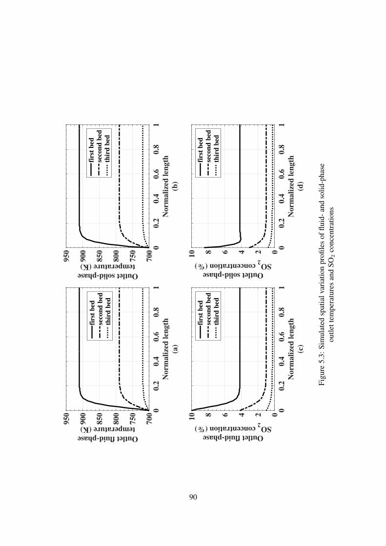
Norm

ali

zed

len

gth

(a)

00.2

0.4

0.6

0.8

1

Outlet fluid-phase

temperature (K) 700

750

800

850

900

950

firs

t b

ed

seco

nd

bed

thir

d b

ed

Norm

ali

zed

len

gth

(b)

00.2

0.4

0.6

0.8

1

Outlet solid-phase

temperature (K) 700

750

800

850

900

950

firs

t b

ed

seco

nd

bed

thir

d b

ed

Norm

ali

zed

len

gth

(c)

00.2

0.4

0.6

0.8

1

Outlet fluid-phase

SO2 concentration (%)

02468

10

firs

t b

ed

seco

nd

bed

thir

d b

ed

Norm

ali

zed

len

gth

(d)

00.2

0.4

0.6

0.8

1

Outlet solid-phase


02468

10

firs

t b

ed

seco

nd

bed

thir

d b

ed

Figu

re5.

3:Si

mul

ated

spat

ialv

aria

tion

profi

les

offlu

id-a

ndso

lid-p

hase

outle

ttem

pera

ture

san

dSO

2co

ncen

trat

ions

90

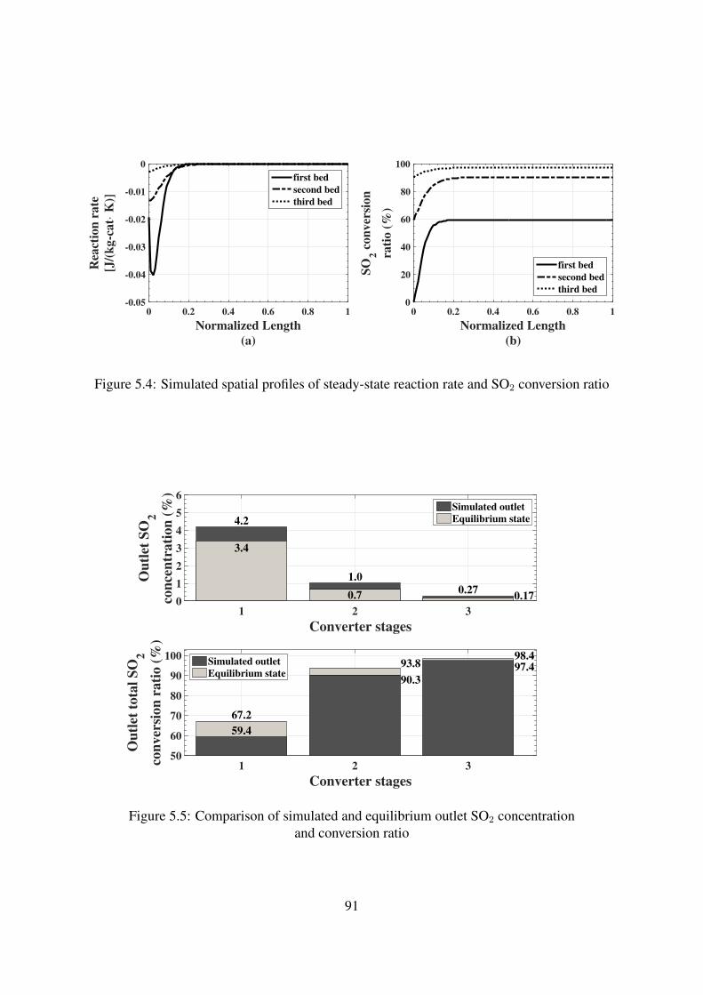
Normalized Length

(a)

0 0.2 0.4 0.6 0.8 1

Rea

ctio

n r

ate

[J/(

kg-c

at·

K)]

-0.05

-0.04

-0.03

-0.02

-0.01

0

first bed

second bed

third bed

Normalized Length

(b)

0 0.2 0.4 0.6 0.8 1

SO

2 c

on

ver

sion

rati

o (

%)

0

20

40

60

80

100

first bed

second bed

third bed

Figure 5.4: Simulated spatial profiles of steady-state reaction rate and SO2 conversion ratio

Converter stages

1 2 3

Ou

tlet

SO

2

con

cen

trati

on

(%

)

0

1

2

3

4

5

6

4.2

1.0

0.27

3.4

0.7 0.17

Simulated outlet

Equilibrium state

Converter stages

1 2 3

Ou

tlet

tota

l S

O2

con

ver

sion

rati

o (

%)

50

60

70

80

90

100

67.2

93.898.4

59.4

90.3

97.4Simulated outlet

Equilibrium state

Figure 5.5: Comparison of simulated and equilibrium outlet SO2 concentrationand conversion ratio

91

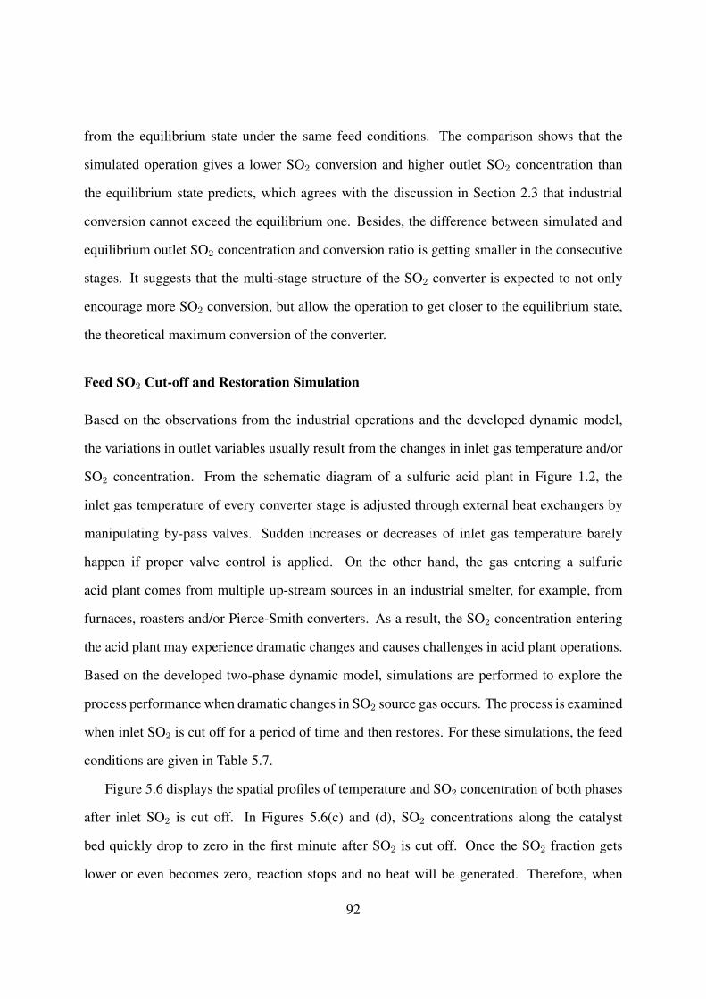
from the equilibrium state under the same feed conditions. The comparison shows that the

simulated operation gives a lower SO2 conversion and higher outlet SO2 concentration than

the equilibrium state predicts, which agrees with the discussion in Section 2.3 that industrial

conversion cannot exceed the equilibrium one. Besides, the difference between simulated and

equilibrium outlet SO2 concentration and conversion ratio is getting smaller in the consecutive

stages. It suggests that the multi-stage structure of the SO2 converter is expected to not only

encourage more SO2 conversion, but allow the operation to get closer to the equilibrium state,

the theoretical maximum conversion of the converter.

Feed SO2 Cut-off and Restoration Simulation

Based on the observations from the industrial operations and the developed dynamic model,

the variations in outlet variables usually result from the changes in inlet gas temperature and/or

SO2 concentration. From the schematic diagram of a sulfuric acid plant in Figure 1.2, the

inlet gas temperature of every converter stage is adjusted through external heat exchangers by

manipulating by-pass valves. Sudden increases or decreases of inlet gas temperature barely

happen if proper valve control is applied. On the other hand, the gas entering a sulfuric

acid plant comes from multiple up-stream sources in an industrial smelter, for example, from

furnaces, roasters and/or Pierce-Smith converters. As a result, the SO2 concentration entering

the acid plant may experience dramatic changes and causes challenges in acid plant operations.

Based on the developed two-phase dynamic model, simulations are performed to explore the

process performance when dramatic changes in SO2 source gas occurs. The process is examined

when inlet SO2 is cut off for a period of time and then restores. For these simulations, the feed

conditions are given in Table 5.7.

Figure 5.6 displays the spatial profiles of temperature and SO2 concentration of both phases

after inlet SO2 is cut off. In Figures 5.6(c) and (d), SO2 concentrations along the catalyst

bed quickly drop to zero in the first minute after SO2 is cut off. Once the SO2 fraction gets

lower or even becomes zero, reaction stops and no heat will be generated. Therefore, when

92

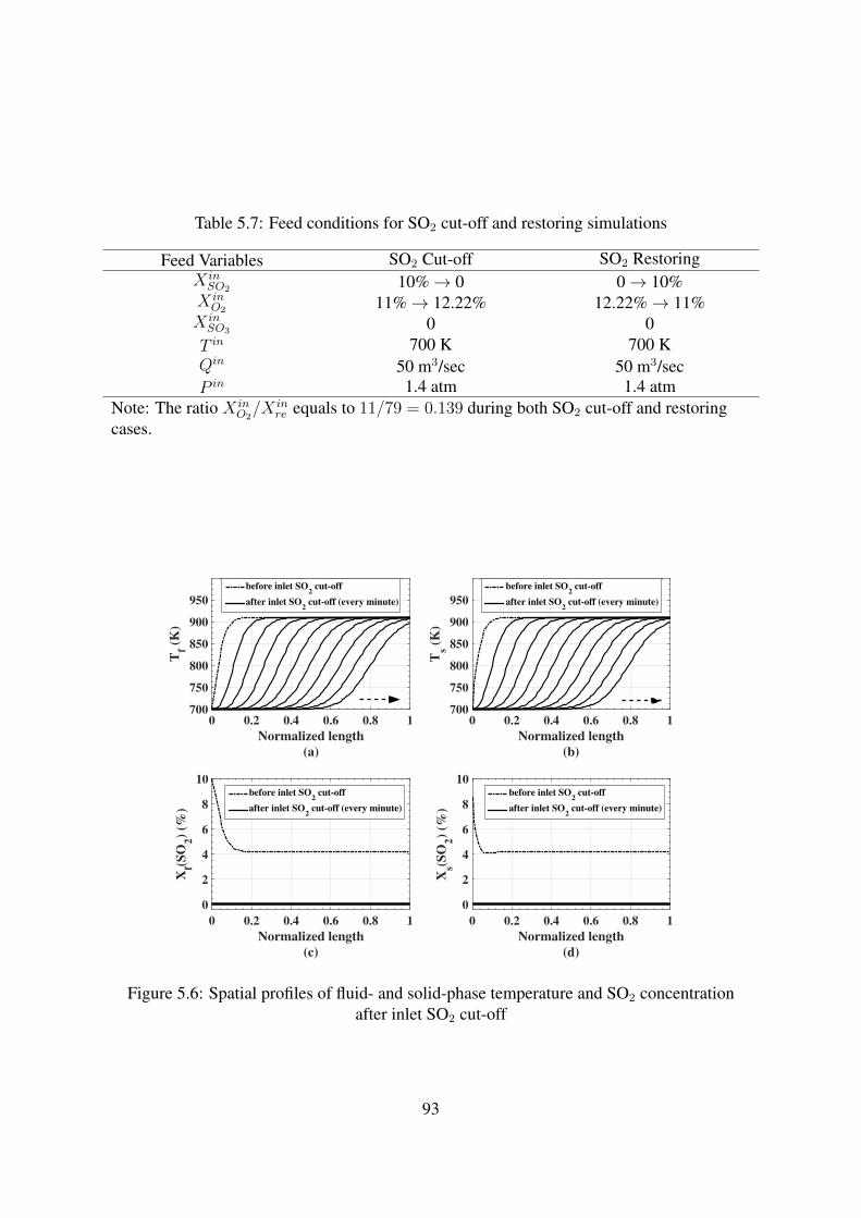
Table 5.7: Feed conditions for SO2 cut-off and restoring simulations

Feed Variables SO2 Cut-off SO2 RestoringX inSO2 10%→ 0 0→ 10%X inO2 11%→ 12.22% 12.22%→ 11%

X inSO3 0 0T in 700 K 700 KQin 50 m3/sec 50 m3/secP in 1.4 atm 1.4 atm

Note: The ratio X inO2/X in

re equals to 11/79 = 0.139 during both SO2 cut-off and restoringcases.

Normalized length

(a)

0 0.2 0.4 0.6 0.8 1

Tf (

K)

700

750

800

850

900

950

before inlet SO2 cut-off

after inlet SO2 cut-off (every minute)

Normalized length

(b)

0 0.2 0.4 0.6 0.8 1

Ts (

K)

700

750

800

850

900

950



Normalized length

(c)

0 0.2 0.4 0.6 0.8 1

Xf(S

O2)

(%)

0

2

4

6

8

10before inlet SO

2 cut-off


Normalized length

(d)

0 0.2 0.4 0.6 0.8 1

Xs(S

O2)

(%)

0

2

4

6

8

10before inlet SO

2 cut-off


Figure 5.6: Spatial profiles of fluid- and solid-phase temperature and SO2 concentrationafter inlet SO2 cut-off

93

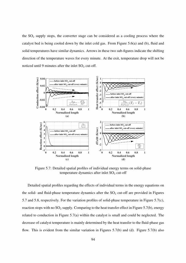
the SO2 supply stops, the converter stage can be considered as a cooling process where the

catalyst bed is being cooled down by the inlet cold gas. From Figure 5.6(a) and (b), fluid and

solid temperatures have similar dynamics. Arrows in these two sub-figures indicate the shifting

direction of the temperature waves for every minute. At the exit, temperature drop will not be

noticed until 9 minutes after the inlet SO2 cut-off.

Normalized length

(a)

0 0.2 0.4 0.6 0.8 1

Con

du

ctio

n e

ffec

t (K

/sec

)

-0.04

-0.02

0

0.02

0.04before inlet SO

2 cut-off


Normalized length

(b)

0 0.2 0.4 0.6 0.8 1Hea

t tr

an

sfer

eff

ect

(K/s

ec)

-6

-5

-4

-3

-2

-1

0

1



Normalized length

(c)

0 0.2 0.4 0.6 0.8 1

Rea

ctio

n e

ffec

t (K

/sec

)

-1

0

1

2

3

4

5

6



Normalized length

(d)

0 0.2 0.4 0.6 0.8 1

dT

s/d

t (K

/sec

)

-3

-2

-1

0

1

2before inlet SO

2 cut-off


kcatρcatcp,cat

·∂2Ts

∂x2

∂Ts

∂t

rhcp,cat

hapρcatcp,cat

(Tf − Ts)

Figure 5.7: Detailed spatial profiles of individual energy terms on solid-phasetemperature dynamics after inlet SO2 cut-off

Detailed spatial profiles regarding the effects of individual terms in the energy equations on

the solid- and fluid-phase temperature dynamics after the SO2 cut-off are provided in Figures

5.7 and 5.8, respectively. For the variation profiles of solid-phase temperature in Figure 5.7(c),

reaction stops with no SO2 supply. Comparing to the heat transfer effect in Figure 5.7(b), energy

related to conduction in Figure 5.7(a) within the catalyst is small and could be neglected. The

decrease of catalyst temperature is mainly determined by the heat transfer to the fluid-phase gas

flow. This is evident from the similar variation in Figures 5.7(b) and (d). Figure 5.7(b) also

94

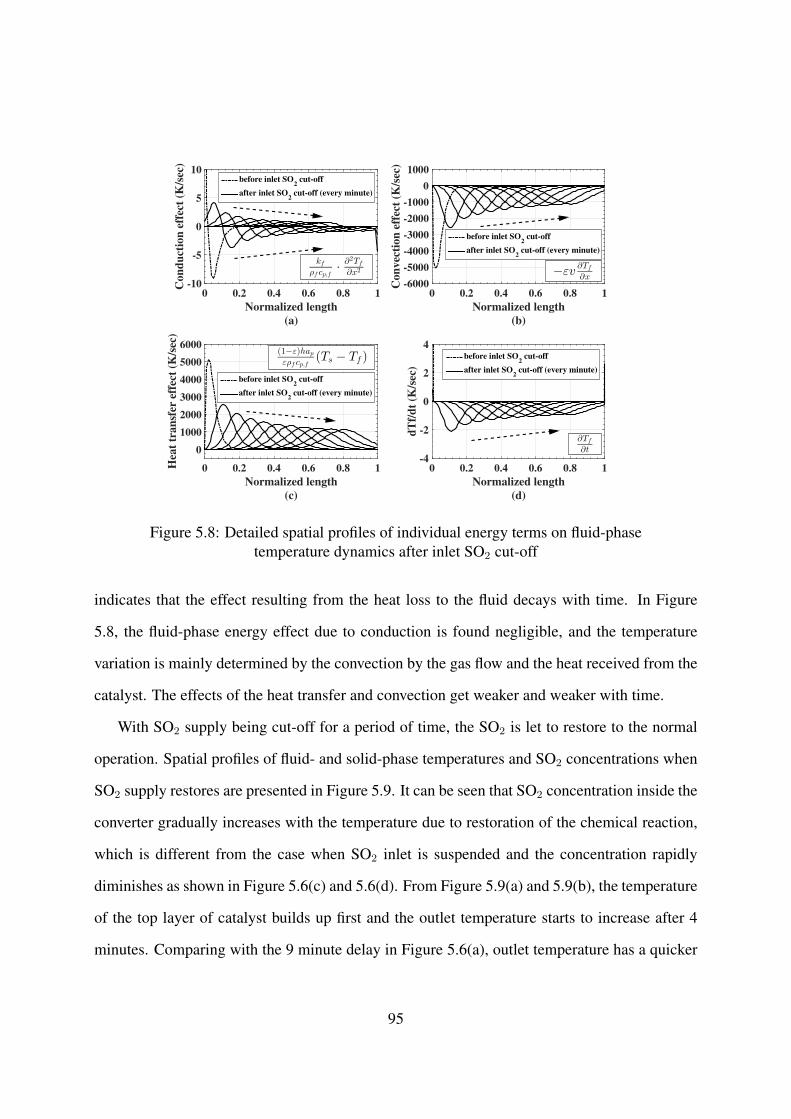
Normalized length

(a)

0 0.2 0.4 0.6 0.8 1

Con

du

ctio

n e

ffec

t (K

/sec

)

-10

-5

0

5

10before inlet SO

2 cut-off


Normalized length

(b)

0 0.2 0.4 0.6 0.8 1

Con

vec

tion

eff

ect

(K/s

ec)

-6000

-5000

-4000

-3000

-2000

-1000

0

1000



Normalized length

(c)

0 0.2 0.4 0.6 0.8 1Hea

t tr

an

sfer

eff

ect

(K/s

ec)

0

1000

2000

3000

4000

5000

6000



Normalized length

(d)

0 0.2 0.4 0.6 0.8 1

dT

f/d

t (K

/sec

)

-4

-2

0

2

4before inlet SO

2 cut-off


kfρf cp,f

·∂2Tf

∂x2 −εv∂Tf

∂x

(1−ε)hapερf cp,f

(Ts − Tf )

∂Tf

∂t

Figure 5.8: Detailed spatial profiles of individual energy terms on fluid-phasetemperature dynamics after inlet SO2 cut-off

indicates that the effect resulting from the heat loss to the fluid decays with time. In Figure

5.8, the fluid-phase energy effect due to conduction is found negligible, and the temperature

variation is mainly determined by the convection by the gas flow and the heat received from the

catalyst. The effects of the heat transfer and convection get weaker and weaker with time.

With SO2 supply being cut-off for a period of time, the SO2 is let to restore to the normal

operation. Spatial profiles of fluid- and solid-phase temperatures and SO2 concentrations when

SO2 supply restores are presented in Figure 5.9. It can be seen that SO2 concentration inside the

converter gradually increases with the temperature due to restoration of the chemical reaction,

which is different from the case when SO2 inlet is suspended and the concentration rapidly

diminishes as shown in Figure 5.6(c) and 5.6(d). From Figure 5.9(a) and 5.9(b), the temperature

of the top layer of catalyst builds up first and the outlet temperature starts to increase after 4

minutes. Comparing with the 9 minute delay in Figure 5.6(a), outlet temperature has a quicker

95

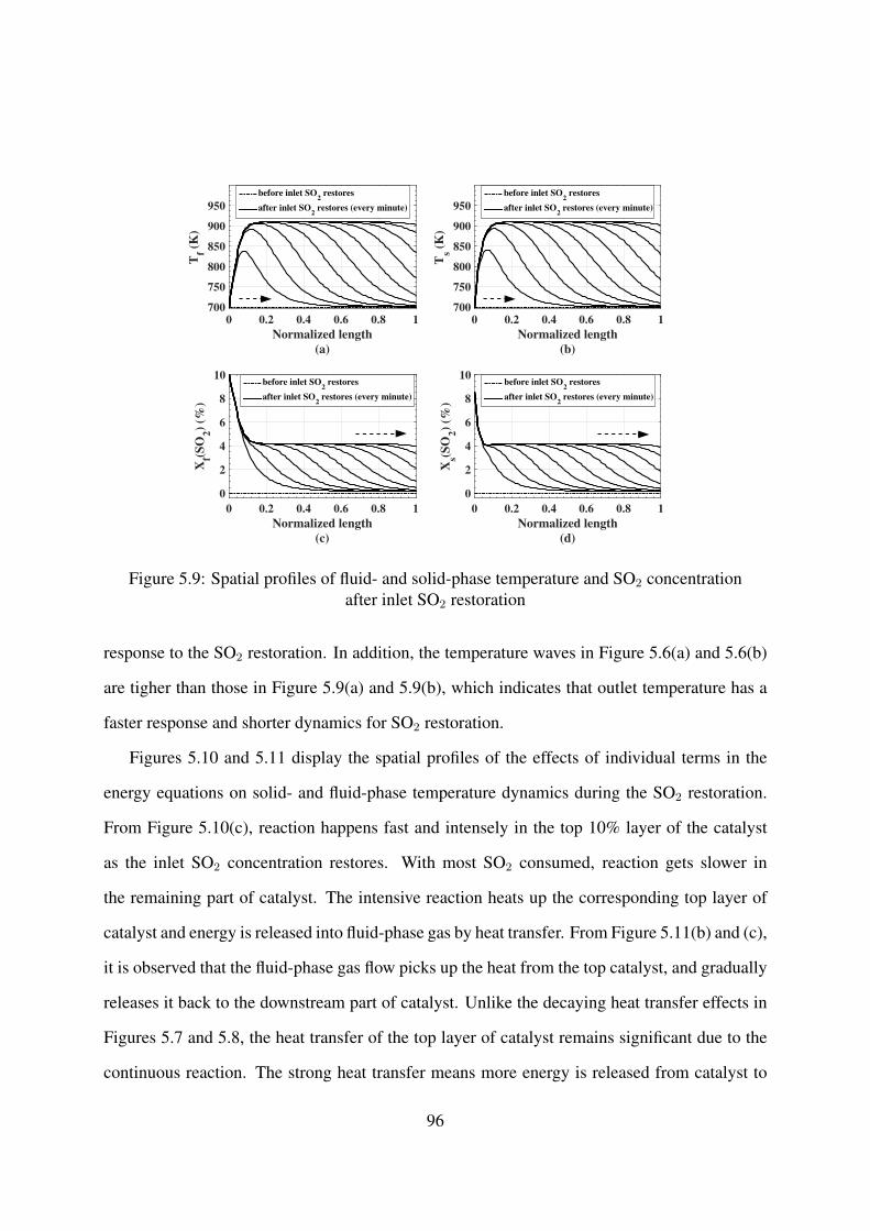
Normalized length

(a)

0 0.2 0.4 0.6 0.8 1

Tf (

K)

700

750

800

850

900

950

before inlet SO2 restores

after inlet SO2 restores (every minute)

Normalized length

(b)

0 0.2 0.4 0.6 0.8 1

Ts (

K)

700

750

800

850

900

950



Normalized length

(c)

0 0.2 0.4 0.6 0.8 1

Xf(S

O2)

(%)

0

2

4

6

8

10before inlet SO

2 restores


Normalized length

(d)

0 0.2 0.4 0.6 0.8 1

Xs(S

O2)

(%)

0

2

4

6

8

10before inlet SO

2 restores


Figure 5.9: Spatial profiles of fluid- and solid-phase temperature and SO2 concentrationafter inlet SO2 restoration

response to the SO2 restoration. In addition, the temperature waves in Figure 5.6(a) and 5.6(b)

are tigher than those in Figure 5.9(a) and 5.9(b), which indicates that outlet temperature has a

faster response and shorter dynamics for SO2 restoration.

Figures 5.10 and 5.11 display the spatial profiles of the effects of individual terms in the

energy equations on solid- and fluid-phase temperature dynamics during the SO2 restoration.

From Figure 5.10(c), reaction happens fast and intensely in the top 10% layer of the catalyst

as the inlet SO2 concentration restores. With most SO2 consumed, reaction gets slower in

the remaining part of catalyst. The intensive reaction heats up the corresponding top layer of

catalyst and energy is released into fluid-phase gas by heat transfer. From Figure 5.11(b) and (c),

it is observed that the fluid-phase gas flow picks up the heat from the top catalyst, and gradually

releases it back to the downstream part of catalyst. Unlike the decaying heat transfer effects in

Figures 5.7 and 5.8, the heat transfer of the top layer of catalyst remains significant due to the

continuous reaction. The strong heat transfer means more energy is released from catalyst to

96

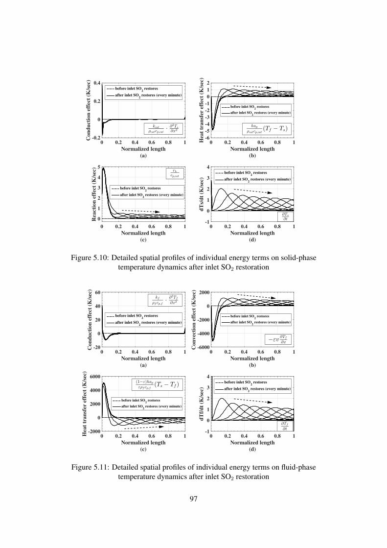
Normalized length

(a)

0 0.2 0.4 0.6 0.8 1

Con

du

ctio

n e

ffec

t (K

/sec

)

-0.2

0

0.2

0.4before inlet SO

2 restores


Normalized length

(b)

0 0.2 0.4 0.6 0.8 1Hea

t tr

an

sfer

eff

ect

(K/s

ec)

-6

-5

-4

-3

-2

-1

0

1

2



Normalized length

(c)

0 0.2 0.4 0.6 0.8 1

Rea

ctio

n e

ffec

t (K

/sec

)

0

1

2

3

4

5



Normalized length

(d)

0 0.2 0.4 0.6 0.8 1

dT

s/d

t (K

/sec

)

-1

0

1

2

3

4before inlet SO

2 restores


kcatρcatcp,cat

·∂2Ts

∂x2hap

ρcatcp,cat(Tf − Ts)

rhcp,cat

∂Ts

∂t

Figure 5.10: Detailed spatial profiles of individual energy terms on solid-phasetemperature dynamics after inlet SO2 restoration

Normalized length

(a)

0 0.2 0.4 0.6 0.8 1

Con

du

ctio

n e

ffec

t (K

/sec

)

-20

0

20

40

60



Normalized length

(b)

0 0.2 0.4 0.6 0.8 1

Con

vec

tion

eff

ect

(K/s

ec)

-6000

-4000

-2000

0

2000



Normalized length

(c)

0 0.2 0.4 0.6 0.8 1Hea

t tr

an

sfer

eff

ect

(K/s

ec)

-2000

0

2000

4000

6000



Normalized length

(d)

0 0.2 0.4 0.6 0.8 1

dT

f/d

t (K

/sec

)

-1

0

1

2

3

4before inlet SO

2 restores


kfρf cp,f

·∂2Tf

∂x2

−εv∂Tf

∂x

(1−ε)hapερf cp,f

(Ts − Tf )

∂Tf

∂t

Figure 5.11: Detailed spatial profiles of individual energy terms on fluid-phasetemperature dynamics after inlet SO2 restoration

97

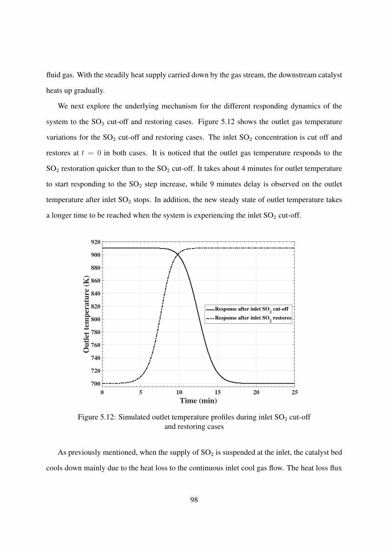
fluid gas. With the steadily heat supply carried down by the gas stream, the downstream catalyst

heats up gradually.

We next explore the underlying mechanism for the different responding dynamics of the

system to the SO2 cut-off and restoring cases. Figure 5.12 shows the outlet gas temperature

variations for the SO2 cut-off and restoring cases. The inlet SO2 concentration is cut off and

restores at t = 0 in both cases. It is noticed that the outlet gas temperature responds to the

SO2 restoration quicker than to the SO2 cut-off. It takes about 4 minutes for outlet temperature

to start responding to the SO2 step increase, while 9 minutes delay is observed on the outlet

temperature after inlet SO2 stops. In addition, the new steady state of outlet temperature takes

a longer time to be reached when the system is experiencing the inlet SO2 cut-off.

Time (min)

0 5 10 15 20 25

Ou

tlet

tem

per

atu

re (

K)

700

720

740

760

780

800

820

840

860

880

900

920

Response after inlet SO2 cut-off

Response after inlet SO2 restores

Figure 5.12: Simulated outlet temperature profiles during inlet SO2 cut-offand restoring cases

As previously mentioned, when the supply of SO2 is suspended at the inlet, the catalyst bed

cools down mainly due to the heat loss to the continuous inlet cool gas flow. The heat loss flux

98

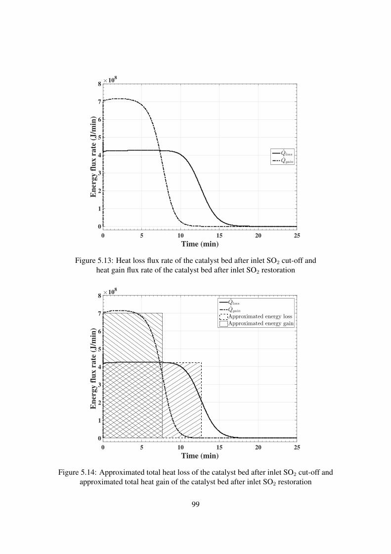
Time (min)

0 5 10 15 20 25

En

ergy f

lux r

ate

(J/m

in)

×108

0

1

2

3

4

5

6

7

8

Qloss

Qgain

Figure 5.13: Heat loss flux rate of the catalyst bed after inlet SO2 cut-off andheat gain flux rate of the catalyst bed after inlet SO2 restoration

Time (min)

0 5 10 15 20 25

En

ergy f

lux r

ate

(J/m

in)

×108

0

1

2

3

4

5

6

7

8Qloss

Qgain

Approximated energy loss

Approximated energy gain

Figure 5.14: Approximated total heat loss of the catalyst bed after inlet SO2 cut-off andapproximated total heat gain of the catalyst bed after inlet SO2 restoration

99

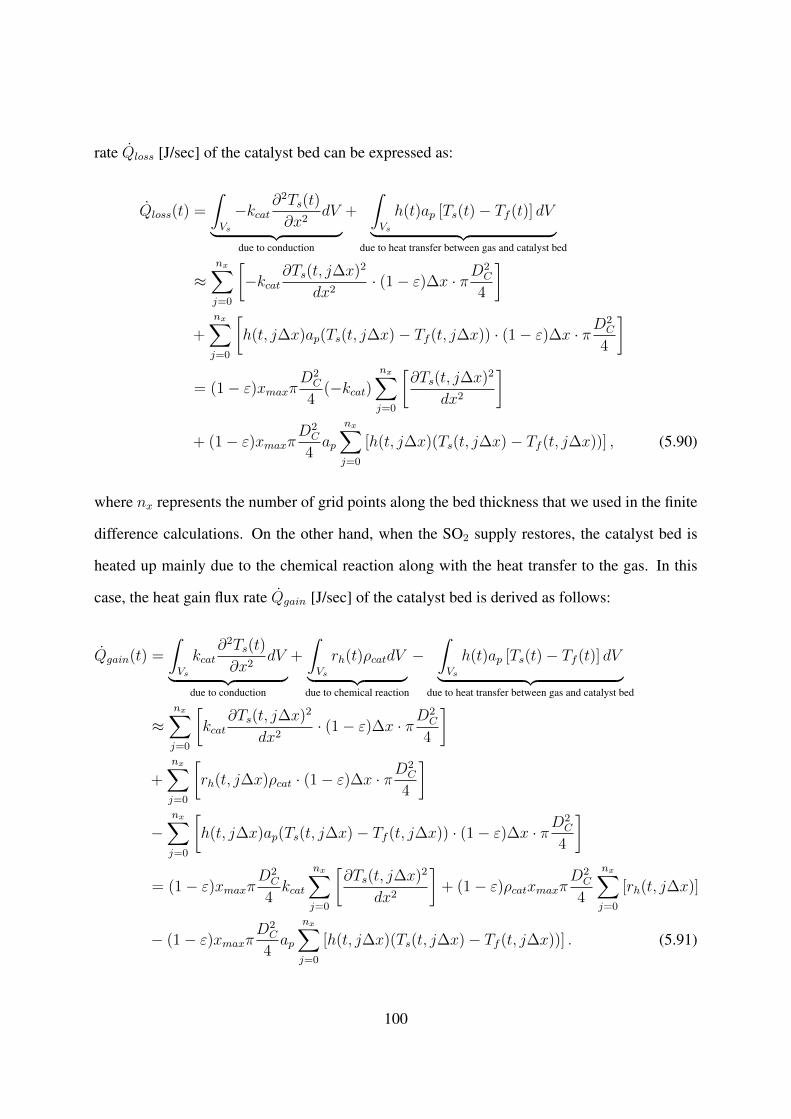
rate Qloss [J/sec] of the catalyst bed can be expressed as:

Qloss(t) =

∫Vs

−kcat∂2Ts(t)

∂x2dV︸︷︷︸

due to conduction

+

∫Vs

h(t)ap [Ts(t)− Tf (t)] dV︸︷︷︸due to heat transfer between gas and catalyst bed

≈nx∑j=0

[−kcat

∂Ts(t, j∆x)2

dx2· (1− ε)∆x · πD

2C

4

]

+nx∑j=0

[h(t, j∆x)ap(Ts(t, j∆x)− Tf (t, j∆x)) · (1− ε)∆x · πD

2C

4

]

= (1− ε)xmaxπD2C

4(−kcat)

nx∑j=0

[∂Ts(t, j∆x)2

dx2

]

+ (1− ε)xmaxπD2C

4ap

nx∑j=0

[h(t, j∆x)(Ts(t, j∆x)− Tf (t, j∆x))] , (5.90)

where nx represents the number of grid points along the bed thickness that we used in the finite

difference calculations. On the other hand, when the SO2 supply restores, the catalyst bed is

heated up mainly due to the chemical reaction along with the heat transfer to the gas. In this

case, the heat gain flux rate Qgain [J/sec] of the catalyst bed is derived as follows:

Qgain(t) =

∫Vs

kcat∂2Ts(t)

∂x2dV︸︷︷︸

due to conduction

+

∫Vs

rh(t)ρcatdV︸︷︷︸due to chemical reaction

−∫Vs

h(t)ap [Ts(t)− Tf (t)] dV︸︷︷︸due to heat transfer between gas and catalyst bed

≈nx∑j=0

[kcat

∂Ts(t, j∆x)2

dx2· (1− ε)∆x · πD

2C

4

]

+nx∑j=0

[rh(t, j∆x)ρcat · (1− ε)∆x · π

D2C

4

]

−nx∑j=0

[h(t, j∆x)ap(Ts(t, j∆x)− Tf (t, j∆x)) · (1− ε)∆x · πD

2C

4

]

= (1− ε)xmaxπD2C

4kcat

nx∑j=0

[∂Ts(t, j∆x)2

dx2

]+ (1− ε)ρcatxmaxπ

D2C

4

nx∑j=0

[rh(t, j∆x)]

− (1− ε)xmaxπD2C

4ap

nx∑j=0

[h(t, j∆x)(Ts(t, j∆x)− Tf (t, j∆x))] . (5.91)

100

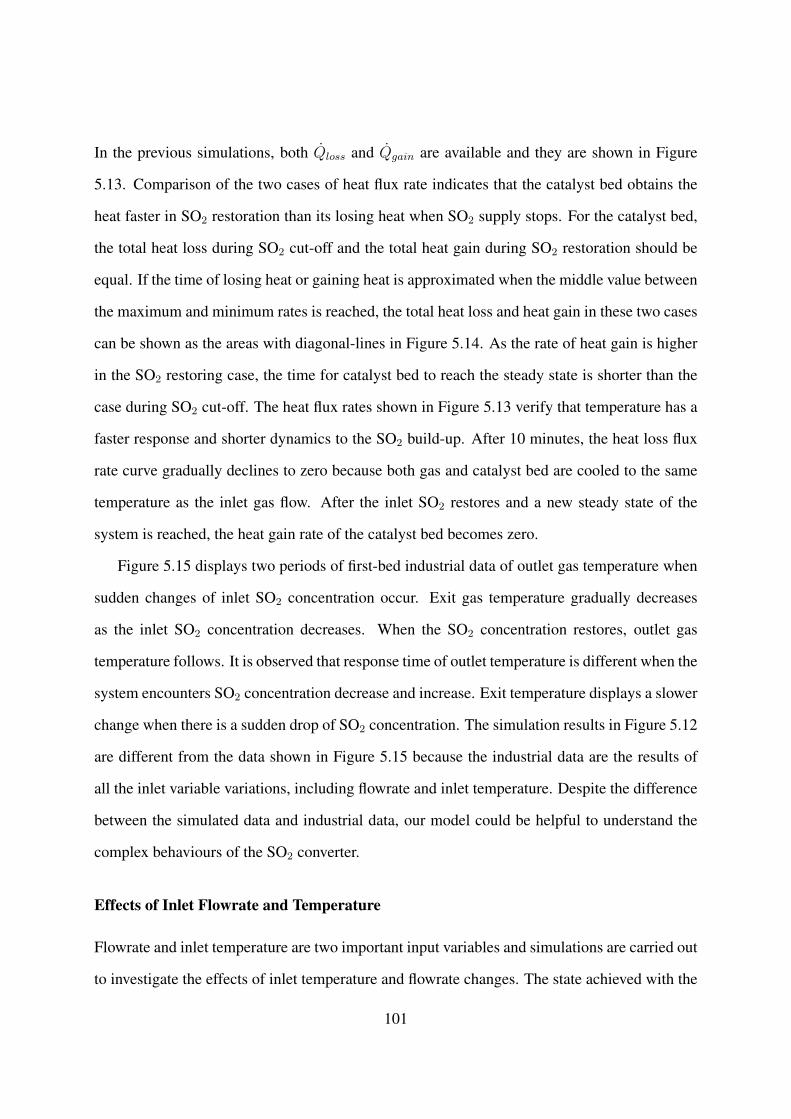
In the previous simulations, both Qloss and Qgain are available and they are shown in Figure

5.13. Comparison of the two cases of heat flux rate indicates that the catalyst bed obtains the

heat faster in SO2 restoration than its losing heat when SO2 supply stops. For the catalyst bed,

the total heat loss during SO2 cut-off and the total heat gain during SO2 restoration should be

equal. If the time of losing heat or gaining heat is approximated when the middle value between

the maximum and minimum rates is reached, the total heat loss and heat gain in these two cases

can be shown as the areas with diagonal-lines in Figure 5.14. As the rate of heat gain is higher

in the SO2 restoring case, the time for catalyst bed to reach the steady state is shorter than the

case during SO2 cut-off. The heat flux rates shown in Figure 5.13 verify that temperature has a

faster response and shorter dynamics to the SO2 build-up. After 10 minutes, the heat loss flux

rate curve gradually declines to zero because both gas and catalyst bed are cooled to the same

temperature as the inlet gas flow. After the inlet SO2 restores and a new steady state of the

system is reached, the heat gain rate of the catalyst bed becomes zero.

Figure 5.15 displays two periods of first-bed industrial data of outlet gas temperature when

sudden changes of inlet SO2 concentration occur. Exit gas temperature gradually decreases

as the inlet SO2 concentration decreases. When the SO2 concentration restores, outlet gas

temperature follows. It is observed that response time of outlet temperature is different when the

system encounters SO2 concentration decrease and increase. Exit temperature displays a slower

change when there is a sudden drop of SO2 concentration. The simulation results in Figure 5.12

are different from the data shown in Figure 5.15 because the industrial data are the results of

all the inlet variable variations, including flowrate and inlet temperature. Despite the difference

between the simulated data and industrial data, our model could be helpful to understand the

complex behaviours of the SO2 converter.

Effects of Inlet Flowrate and Temperature

Flowrate and inlet temperature are two important input variables and simulations are carried out

to investigate the effects of inlet temperature and flowrate changes. The state achieved with the

101

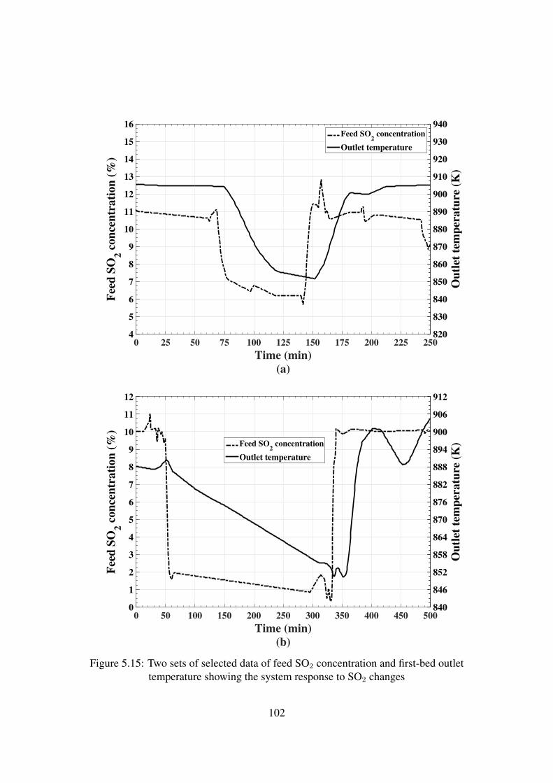
Time (min)

(a)

0 25 50 75 100 125 150 175 200 225 250

Fee

d S

O2 c

on

cen

trati

on

(%

)

4

5

6

7

8

9

10

11

12

13

14

15

16

Ou

tlet

tem

per

atu

re (

K)

820

830

840

850

860

870

880

890

900

910

920

930

940Feed SO

2 concentration

Outlet temperature

Time (min)

(b)

0 50 100 150 200 250 300 350 400 450 500

Fee

d S

O2 c

on

cen

trati

on

(%

)

0

1

2

3

4

5

6

7

8

9

10

11

12

Ou

tlet

tem

per

atu

re (

K)

840

846

852

858

864

870

876

882

888

894

900

906

912

Feed SO2 concentration

Outlet temperature

Figure 5.15: Two sets of selected data of feed SO2 concentration and first-bed outlettemperature showing the system response to SO2 changes

102

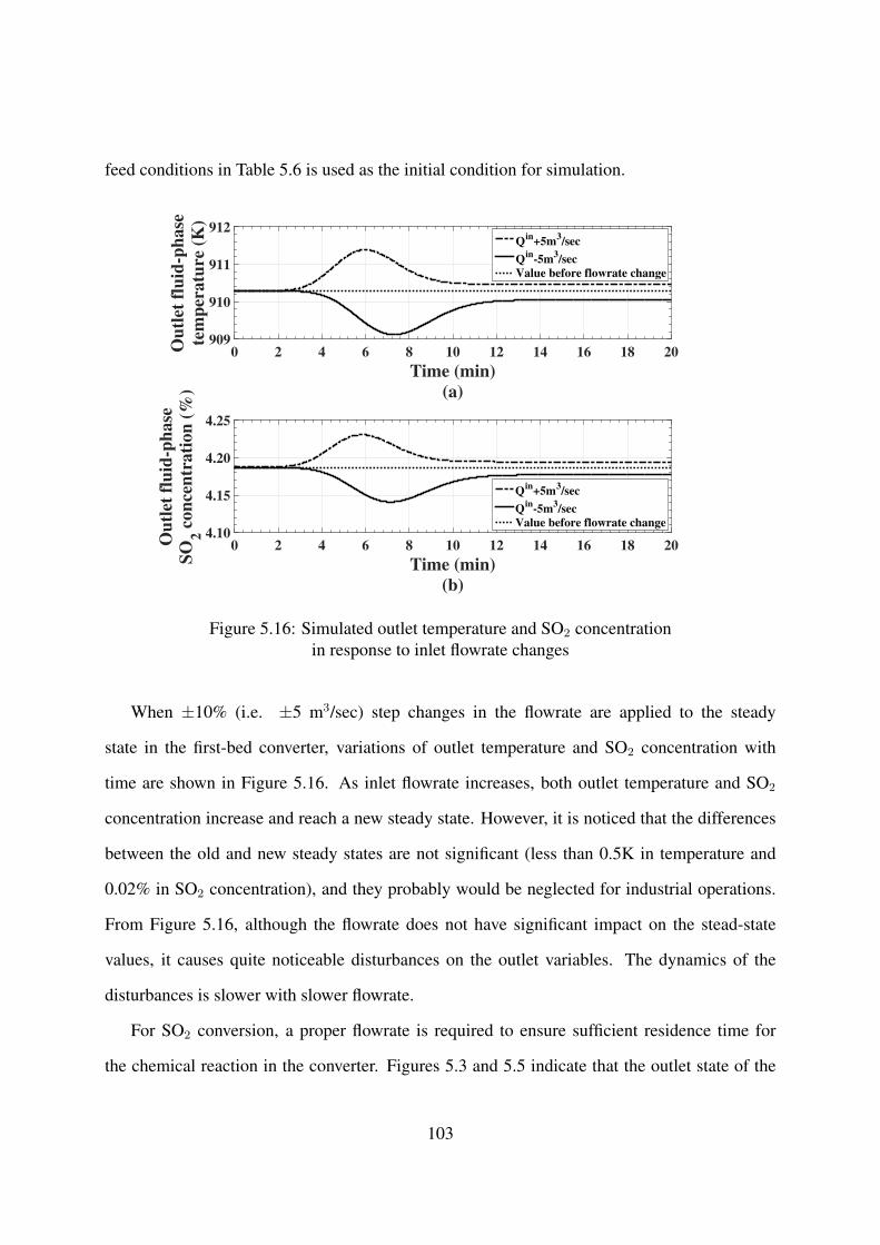
feed conditions in Table 5.6 is used as the initial condition for simulation.

Time (min)

(a)

0 2 4 6 8 10 12 14 16 18 20Ou

tlet

flu

id-p

hase

tem

per

atu

re (

K)

909

910

911

912Q

in+5m

3/sec

Qin

-5m3/sec

Value before flowrate change

Time (min)

(b)

0 2 4 6 8 10 12 14 16 18 20Ou

tlet

flu

id-p

hase

SO

2 c

on

cen

trati

on

(%

)

4.10

4.15

4.20

4.25

Qin

+5m3/sec

Qin

-5m3/sec


Figure 5.16: Simulated outlet temperature and SO2 concentrationin response to inlet flowrate changes

When ±10% (i.e. ±5 m3/sec) step changes in the flowrate are applied to the steady

state in the first-bed converter, variations of outlet temperature and SO2 concentration with

time are shown in Figure 5.16. As inlet flowrate increases, both outlet temperature and SO2

concentration increase and reach a new steady state. However, it is noticed that the differences

between the old and new steady states are not significant (less than 0.5K in temperature and

0.02% in SO2 concentration), and they probably would be neglected for industrial operations.

From Figure 5.16, although the flowrate does not have significant impact on the stead-state

values, it causes quite noticeable disturbances on the outlet variables. The dynamics of the

disturbances is slower with slower flowrate.

For SO2 conversion, a proper flowrate is required to ensure sufficient residence time for

the chemical reaction in the converter. Figures 5.3 and 5.5 indicate that the outlet state of the

103

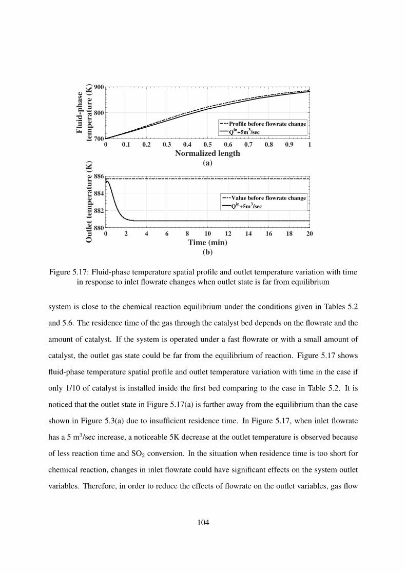
Normalized length

(a)

0 0.1 0.2 0.3 0.4 0.5 0.6 0.7 0.8 0.9 1

Flu

id-p

hase

tem

per

atu

re (

K)

700

800

900

Profile before flowrate change

Qin

+5m3/sec

Time (min)

(b)

0 2 4 6 8 10 12 14 16 18 20

Ou

tlet

tem

per

atu

re (

K)

880

882

884

886


Qin

+5m3/sec

Figure 5.17: Fluid-phase temperature spatial profile and outlet temperature variation with timein response to inlet flowrate changes when outlet state is far from equilibrium

system is close to the chemical reaction equilibrium under the conditions given in Tables 5.2

and 5.6. The residence time of the gas through the catalyst bed depends on the flowrate and the

amount of catalyst. If the system is operated under a fast flowrate or with a small amount of

catalyst, the outlet gas state could be far from the equilibrium of reaction. Figure 5.17 shows

fluid-phase temperature spatial profile and outlet temperature variation with time in the case if

only 1/10 of catalyst is installed inside the first bed comparing to the case in Table 5.2. It is

noticed that the outlet state in Figure 5.17(a) is farther away from the equilibrium than the case

shown in Figure 5.3(a) due to insufficient residence time. In Figure 5.17, when inlet flowrate

has a 5 m3/sec increase, a noticeable 5K decrease at the outlet temperature is observed because

of less reaction time and SO2 conversion. In the situation when residence time is too short for

chemical reaction, changes in inlet flowrate could have significant effects on the system outlet

variables. Therefore, in order to reduce the effects of flowrate on the outlet variables, gas flow

104

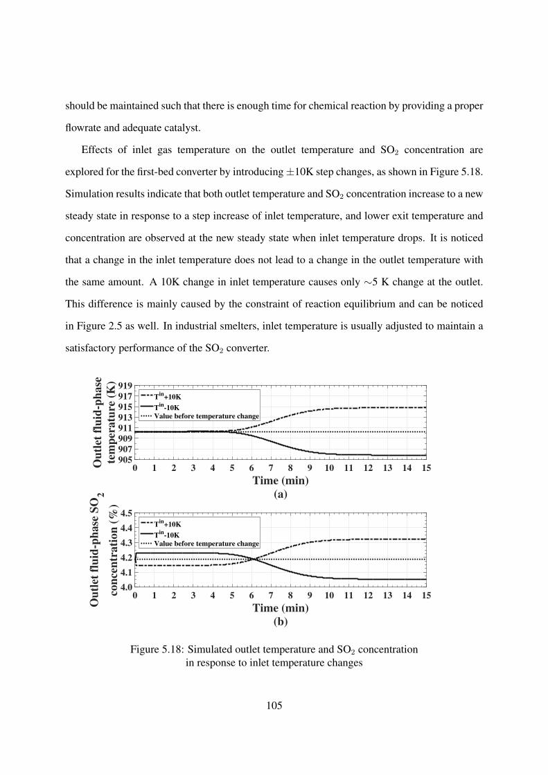
should be maintained such that there is enough time for chemical reaction by providing a proper

flowrate and adequate catalyst.

Effects of inlet gas temperature on the outlet temperature and SO2 concentration are

explored for the first-bed converter by introducing±10K step changes, as shown in Figure 5.18.

Simulation results indicate that both outlet temperature and SO2 concentration increase to a new

steady state in response to a step increase of inlet temperature, and lower exit temperature and

concentration are observed at the new steady state when inlet temperature drops. It is noticed

that a change in the inlet temperature does not lead to a change in the outlet temperature with

the same amount. A 10K change in inlet temperature causes only ∼5 K change at the outlet.

This difference is mainly caused by the constraint of reaction equilibrium and can be noticed

in Figure 2.5 as well. In industrial smelters, inlet temperature is usually adjusted to maintain a

satisfactory performance of the SO2 converter.

Time (min)

(a)

0 1 2 3 4 5 6 7 8 9 10 11 12 13 14 15Ou

tlet

flu

id-p

hase

tem

per

atu

re (

K)

905

907

909

911

913

915

917

919T

in+10K

Tin

-10K

Value before temperature change

Time (min)

(b)

0 1 2 3 4 5 6 7 8 9 10 11 12 13 14 15

Ou

tlet

flu

id-p

hase

SO

2

con

cen

trati

on

(%

)

4.0

4.1

4.2

4.3

4.4

4.5T

in+10K

Tin

-10K

Value before temperature change

Figure 5.18: Simulated outlet temperature and SO2 concentrationin response to inlet temperature changes

105

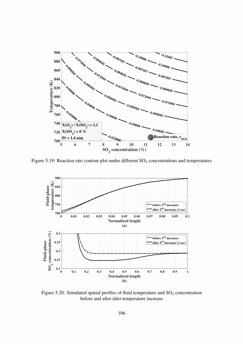
-0.12267

-0.10999

-0.10999

-0.097307

-0.097307

-0.097307

-0.084625

-0.084625

-0.084625

-0.084625

-0.071944

-0.071944

-0.071944

-0.071944

-0.071944

-0.059262

-0.059262

-0.059262

-0.059262

-0.059262

-0.04658

-0.04658

-0.04658

-0.04658

-0.04658

-0.033898

-0.033898

-0.033898

5 6 7 8 9 10 11 12 13 14


700

720

740

760

780

800

820

840

860

880

900T

emp

eratu

re (

K)

Reaction rate, rSO2

X(O2) / X(SO

2) = 1.1

X(SO3) = 0 %

Pt = 1.4 atm

Figure 5.19: Reaction rate contour plot under different SO2 concentrations and temperatures

Normalized length

(a)

0 0.01 0.02 0.03 0.04 0.05 0.06 0.07 0.08 0.09 0.1

Flu

id-p

hase

tem

per

atu

re (

K)

700

750

800

850

900

before Tin

increases

after Tin

increases (1 sec)

Normalized length

(b)

0 0.1 0.2 0.3 0.4 0.5 0.6 0.7 0.8 0.9 1

Flu

id-p

hase

SO

2 c

on

cen

trati

on

(%

)

4.1

4.15

4.2

4.25

4.3

before Tin

increases

after Tin

increases (1 sec)

Figure 5.20: Simulated spatial profiles of fluid temperature and SO2 concentrationbefore and after inlet temperature increase

106

In Figure 5.18, The outlet temperature displays 5 minute time delay response. For SO2

concentration, however, it responds to the inlet temperature changes almost simultaneously. As

the inlet temperature increases, the SO2 concentration decreases. We attempt to explore the

mechanism behind the above observations from the dependence of reaction rate on the SO2

concentration and gas temperature. Figure 5.19 presents the reaction rate contour regarding the

SO2 concentration and temperature. For a given SO2 concentration, higher temperature is found

to favor the reaction and lead to a higher reaction rate. Therefore, when a step increase occurs

at the inlet temperature, reaction rate speeds up and more SO2 is consumed at the top layer of

catalyst leading to SO2 concentration decrease.

Figure 5.20 show the spatial profiles of fluid temperature and SO2 concentration in the

converter stage when inlet temperature has a step increase. From Figure 5.20(b), after 1 second,

the effect of SO2 concentration decrease has been carried down by the gas flow and covered

the top 80% of the catalyst. On the other hand, temperature increase is limited in the 10%

of catalyst, as shown in Figure 5.20(a). Consequently, when feed temperature has a step

increase of 10K, outlet SO2 concentration experiences a fast drop almost simultaneously but

outlet temperature remains constant for the first 5 minutes as shown in Figure 5.18. When the

outlet temperature gradually escalates afterwards, outlet SO2 concentration follows the change

and a new steady state is reached. By observing the differential Equations (5.53 - 5.60), it is

noticed that the heat capacity coefficient (ρcp) of the catalyst is larger than that of the fluid gas,

leading to the slower variation of temperature comparing to those of the concentrations.

5.5 Industrial Data Comparison

At last, the two-phase dynamic model for the SO2 catalytic converter is used to simulate some

more realistic situations. With the estimated parameters in Section 5.3, one period of the

industrial feed data are used as the feed conditions, and the process performance is simulated.

The simulated outlet gas temperature of four converter stages is compared with the measured

107

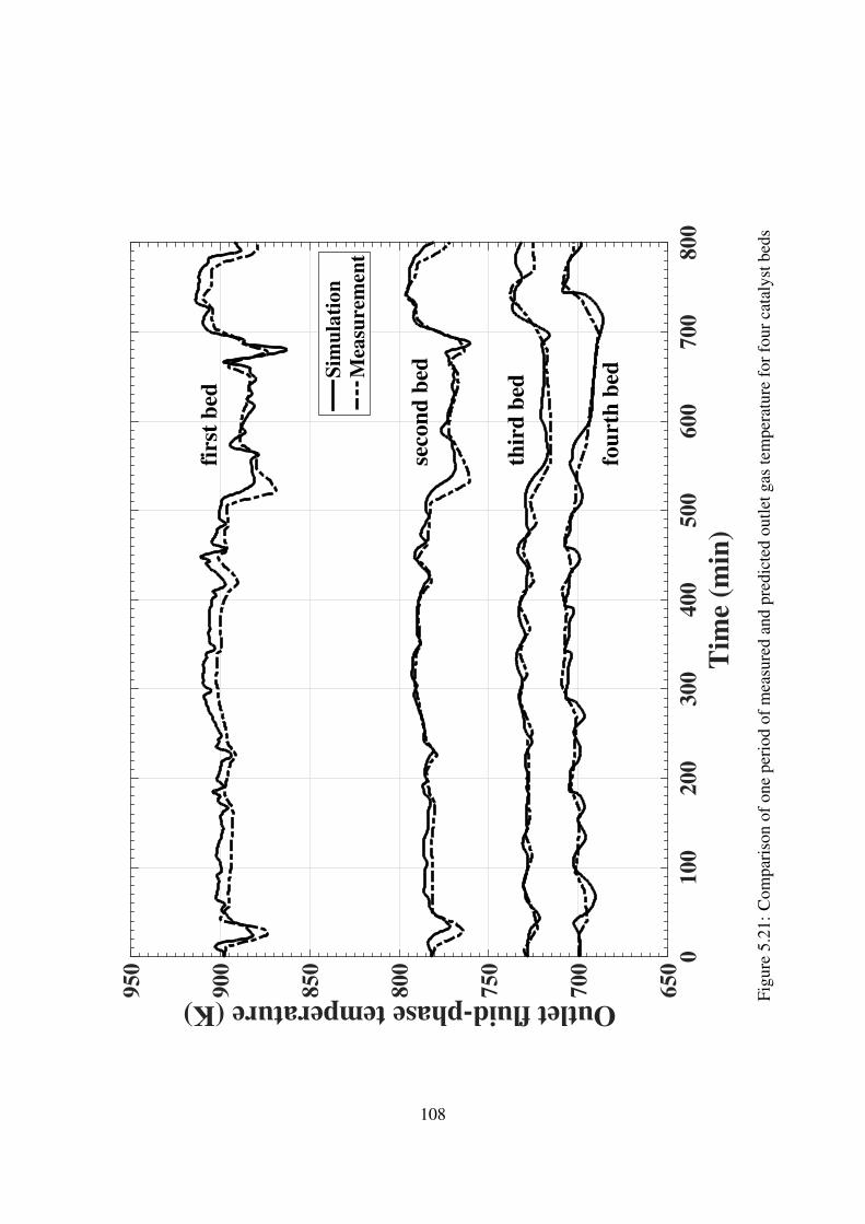
Tim

e (m

in)

0100

200

300

400

500

600

700

800

Outlet fluid-phase temperature (K) 650

700

750

800

850

900

950

firs

t b

ed

seco

nd

bed

thir

d b

ed

fou

rth

bedS

imu

lati

on

Mea

sure

men

t

Figu

re5.

21:C

ompa

riso

nof

one

peri

odof

mea

sure

dan

dpr

edic

ted

outle

tgas

tem

pera

ture

forf

ourc

atal

ystb

eds

108

temperature in Figure 5.21. It is observed that the simulated outlet gas temperature tracks

the measurements reasonably well when the measurement varies slowly. This indicates that

the model has a good validity in describing the industrial system. Existence of mismatch

between the simulated temperature and the measurements is reasonable as the mechanistic

model contains many parameters that can only approximately be estimated, while the industrial

system may have unknown noises. In addition, other factors can also contribute to the mismatch,

such as the neglected heat loss of the converter to the environment, the channelling effect in

the catalyst bed, missing information about the oxygen concentrations from the collected data,

and/or inaccurate estimated parameters.

5.6 Summary

In order to have a better understanding of the SO2 conversion process, detailed modelling on

the SO2 converter is necessary. This chapter develops the dynamic model by applying the

mass and energy conservations on both fluid- and solid-phase gas mixtures. This developed

two-phase dynamic model takes the form of partial differential equations (PDE) and provides

a mathematical tool to explore the interaction between gas flow and catalyst during normal

industrial operation.

Based on the proposed model, simulations are run to examine the spatial variations of

the temperatures and SO2 concentrations within three SO2 converter stages under given feed

conditions. It shows that chemical reaction mainly occurs in the top layer of the catalyst beds.

Comparisons are also given between the simulated and equilibrium outlet SO2 concentrations

and conversion ratios.

The SO2 cut-off and restoring cases are simulated by the developed two-phase model.

Simulation results provide the detailed two-phase temperature and SO2 concentration spatial

profiles varying with time. Studies indicate that SO2 concentration diminishes quickly after

SO2 is cut-off and then the catalyst temperature decreases only through gradual heat loss to the

109

gas stream. The cold inlet gas continuously carries the released energy away and eventually

cools down the catalyst bed. As for SO2 supply restoring case, intensive reaction occurs at the

top layer of catalyst and energy is continuously discharged from catalyst to gas flow by heat

transfer. The heated gas flow delivers the energy into downstream and heats up the subsequent

catalyst through energy exchange. Comparison between the heat loss flux rate after SO2 stops

and the heat gain flux rate from reaction after SO2 restores indicates that the catalyst bed receives

the reaction heat faster and speeds up the restoring process. Industrial data are examined and

similar variation exists in variable dynamics.

Effects of the inlet flowrate and temperature are investigated using the developed PDE

model. The simulation results show that changes in inlet flowrate barely affect the outlet

steady states of temperature and SO2 concentration, but affect the responding time delay and

the variation speed of the system. With an inlet temperature increase, new higher steady state is

observed in the outlet temperature and SO2 concentration. The steady-state gain ratio of outlet

to inlet temperatures is found around 0.5. The outlet SO2 concentration is noticed to have a

faster response to the feed temperature changes than the outlet temperature because the heat

capacity difference between the gas and catalyst defers the energy variations.

With the estimated parameters, outlet gas temperature is predicted through dynamic

simulations using the two-phase model with collected feed data. The prediction results show a

good match with the industrial measurements.

110

Chapter 6

Conclusions and Future Work

Sulfuric acid plants that capture SO2 from industrial off-gas emissions are essential for the

modern process industry. The core unit is the catalytic SO2 converter as this determines SO2

conversion and, therefore, sulfuric acid production.

The focus of this thesis is to develop mathematical models for SO2 converters for various

applications. The developed models will be used to describe the performance of SO2 converters

and provide a fundamental tool for future process analysis, optimization and control.

6.1 Conclusions

In Chapter 2, steady-state modelling of the catalytic SO2 converter is carried out based on

steady-state mass and energy conservation. The obtained steady-state model provides an

explicit relation between the SO2 conversion ratio and gas temperature. This steady-state

relationship is used to generate a heat-up path. By combining the heat-up path with the

equilibrium curve of reaction (1.2), the equilibrium SO2 conversion ratio and temperature can

be calculated. The equilibrium conversion ratio reflects the theoretical maximum conversion

which a SO2 converter can achieve under given feed conditions. A heat-up path simulation is

performed on a three-stage converter and the results indicate that the majority of conversion

111

is in the first catalyst bed. Heat-up paths under different inlet gas temperatures and SO2

concentrations are explored and the proposed steady-state models should serve as a tool for

the dynamic modelling and simplification.

SO2 concentration and conversion ratio are important variables for the SO2 converter

operation, but they are little measured in many smelters due to hardware constraints. Chapter

3 established mathematical soft sensors for these essential variables so that they can be

estimated from available measured variables. The soft sensors are built based on the steady-

state models and industrial dynamic data analysis. From the industrial data, correlation

examination discovers that outlet gas temperature is highly related to the inlet SO2 concentration

and the maximum correlation coefficient is derived when delay time equals to 9 minutes.

A first-order exponential data filter is introduced and applied to the inlet SO2 data to

achieve the synchronization with outlet temperature. Using the filter’s SO2 concentration

signals, the mathematical soft sensors generate a reasonable and useful estimation of outlet

SO2 concentration and conversion ratio. This provides helpful information to examine the

performance of the converter.

A dynamic model of the SO2 converter is obtained in Chapter 4 using dynamic mass and

energy conservation. This developed dynamic model takes the form of ordinary differential

equations (ODE) and uses the SO2 conversion ratio as a key variable in the model development.

In comparison with existing models, introducing the SO2 conversion ratio into modelling avoids

the necessity of reaction kinetics knowledge or expressions which sometimes are difficult to

confirm due to too many parameters. Outlet gas temperature is predicted by the ODE model

based on the available feed data. Comparison between the collected industrial measurements

and prediction verifies the validity of the proposed model in describing the converter. With the

proposed dynamic model, simulations are carried out to explore the effects of input variables.

Inlet flowrate is found to effect the system dynamic speed, while outlet gas temperature exhibits

slow dynamics in relation to inlet SO2 changes. In addition, through steady-state observations,

112

a higher inlet SO2 concentration results in more SO2 conversion, but a lower SO2 conversion

ratio. This dynamic model incorporating the SO2 conversion ratio can be conveniently applied

to many SO2 converters with easy parameter estimation using available operating data. It could

be also used as the base equations for design when process control enhancement is required for

the converters.

Detailed dynamic modelling is performed on the SO2 converters by implementing mass

and energy continuities on both fluid- and solid-phase gas mixtures. The two-phase dynamic

model, established in the form of partial differential equations (PDE), is able to describe the

SO2 converter with time and space. In contrast with the existing dynamic models of the

converters, difference between gas and catalyst temperature changes is considered so that the

energy interaction between gas and catalyst can be studied. With the evaluated parameters,

industrial feed data are applied to the two-phase dynamic model to produce a prediction of

outlet gas temperature. The prediction fits well with industrial measurement and thus validates

the detailed dynamic model.

Spatial variations of the fluid- and solid-phase temperatures and SO2 concentrations in three-

stage SO2 converter are generated by dynamic simulations with the two-phase model. Chemical

reaction is found to happen within the top layer of catalyst beds. Comparison between the

simulated and equilibrium outlet SO2 concentrations, and conversion ratios, are provided and

the results show that the simulated conversion cannot exceed the equilibrium.

Simulations are carried out to explore the feed SO2 cut-off and restoring cases and their

effects. When inlet SO2 cut-off occurs, SO2 concentration inside the converter rapidly falls by

flow and chemical reaction. The decline of both gas and catalyst temperatures in the converter

are observed and their variations are determined by the energy transfer between gas and catalyst

along with the continuous inlet gas flow. Effect of energy transfer gradually dies out with time,

leading to the slow dynamics of the gas temperature. For inlet SO2 supply restoration, fast

reaction happens within the top layer of the catalyst bed, and this strengthens energy transfer

113

from the catalyst to the gas. The gas flow carries the received energy down to subsequent

catalyst and releases it back to the catalyst. With the constantly fast reaction at the top catalyst

layer, the strengthened energy transfer and gas movements lead to fast dynamics in outlet

temperature in comparison with the case when the SO2 cut-off occurs. By comparing the heat

loss flux rate of the catalyst bed for SO2 cut-off and the heat gain flux rate of the catalyst bed

for SO2 restoration, it is noted that the catalyst bed absorbs the reaction heat from the restored

reaction faster than it losing heat when SO2 is cut off. This heat flux rate difference directly

leads to the fast response dynamics on the outlet temperature when the SO2 restoration occurs.

Simulations show that the developed two-phase model provides clear and detailed profiles of

the SO2 converter behaviour. Observation from the industrial data shows a similar response and

dynamic pattern for the outlet temperature to SO2 concentration changes.

The proposed detailed dynamic model is also used to investigate the effects of inlet flowrate

and temperature on the SO2 converter outlet. From the simulation results, inlet flowrate

variations, as typically happens in industrial operations, hardly impact outlet steady states.

System response time delay and dynamics, on the other hand, are significantly impacted by

flowrate changes. Inlet temperature changes causes variations on the outlet temperature and

SO2 concentration. Higher steady-state outlet temperature and SO2 concentration are obtained

as a result of a feed temperature increase. The outlet SO2 concentration is found to almost

simultaneously respond to the sudden changes in inlet temperature.

6.2 Future Work

Modelling of the catalytic SO2 converter is important for sulfuric acid plant control. A good

model on the SO2 converter is presented to provide valuable information while describing the

behaviour of the converting process and can eventually help with improvement of the sulfuric

acid plant. In this thesis, detailed dynamic modelling has been performed on the SO2 converters,

including steady-state model, dynamic model in the form of ODE incorporating with SO2

114

conversion ratio, and detailed PDE dynamic model dividing the gas mixture into two phases.

Based on the current work, there are still some open problems and investigations that may be

addressed for by future research.

In this thesis, a dynamic model is established by using the SO2 conversion ratio as the key

variable. In order to connect the SO2 conversion ratio only with the inlet variables, a linear

relation is proposed between the actual and equilibrium conversion ratios. Even though the

proposed dynamic model gives a good match with the data, challenges still remain to establish

a more accurate relation between the actual and equilibrium conversion ratios. Achieving this

will eventually improve the performance of the dynamic model, as well as the SO2 conversion

ratio estimation.

The detailed two-phase dynamic models in this thesis contain many process parameters.

Most of them are estimated based on empirical expressions from existing work. Estimation of

a large number of unknown parameters from a set of partial differential equations is always

challenging. Especially for the kinetics parameters in the reaction rate expression, they should

be varied if different catalyst is applied. A good estimation of the parameters will improve the

accuracy of the dynamic model and extend its applications.

For a SO2 converter located in a sulfuric acid plant within an industrial smelter,

process control development is always important and necessary to deal with varying process

disturbances. A stable and constantly high conversion of SO2 is beneficial to acid product

production. Control strategy investigation will, therefore, be necessary in future research.

115

ReferencesM. Amazouz and R. Platon. Soft-sensors for real-time monitoring and control of a black liquor

concentration process. In Proceedings of the 2011 International Conference on Data Mining,

pages 22 – 27, 2011.

G. Amhalhel and P. Furmanski. Problems of modeling flow and heat transfer in porous media.

Journal of Power Technologies, 85:55 –88, 1997.

A. Amiri and K. Vafai. Analysis of dispersion effects and non-thermal equilibrium, non-darcian,

variable porosity incompressible flow through porous media. International Journal of Heat

and Mass Transfer, 37:939 – 954, 1994.

N.G. Ashar and K.R. Golwalkar. A practical guild to the manufacture of sulfuric acid, oleums,

and sulfonating agents. Springer INternational Publishing, 2013.

A. Bousri, K. Bouhadef, H. Beji, R. Bennacer, and R. Nebbali. Heat and mass transfer in

reactive porous media with local nonequilibrium conditions. Journal of Porous Media, 15:

329 – 341, 2012.

H. Byrdziak, J. Dobrzanski, J. Garbaczewski, and J. Kotarski. Sulfur dioxide emission reduction

by the polish copper industry. In Proceeding of the 1996 125th TMS Annual Meeting, pages

1005 – 1013, 1996.

W.H. Chan, R.J. Vet, Chul-Un Ro, A.J.S. Tang, and M.A. Lusis. Impact of INCO smelter

emissions on wet and dry deposition on the sudbury area. Atmospheric Environment, 18(5),

1984a.

W.H. Chan, R.J. Vet, Chul-Un Ro, A.J.S. Tang, and M.A. Lusis. Long-term precipitation quality

and wet deposition fields in the Sudbury Basin. Atmospheric Environment, 18(6):1175 –

1188, 1984b.

116

Jr. Chase, M.W. Nist-janaf themochemical tables, fourth edition. Journal of Physical and

Chemical Reference Data, Monograph 9, pages 1–1951, 1998.

A. Ciccone and J. Storbeck. Fugitive SO2 and particulate emissions from a smelter complex.

In Proceedings of the Air & Waste Management Association’s Annual Meeting & Exhibition,

1997.

A.K. Coker. Ludwig’s applied process design for chemical and petrochemical plants, 2007.

H. Darcy. Les fontaines publiques de la ville de dijon, 1856.

W.G. Davenport and M.J. King. Sulphuric Acid Manufacture. Elsevier, 2006.

A. Di Bella, L. Fortuna, S. Graziani, G. Napoli, and M.G. Xibilia. Soft sensor design for a

sulfur recovery unit using genetic algorithms. In 2007 IEEE International Symposium on

Intelligent Signal Processing, WISP, 2007.

D. Dong, T.J. McAvoy, and L.J. Chang. Emission monitoring using multivariate soft sensors.

In Proceedings of the 1995 American Control Conference, volume 1, pages 761 – 765, 1995.

J.R. Donovan, J.S. Palermo, and R.M. Smith. Sulfuric acid converter optimization. CEP

(Chemical Engineering Progress), 74(9):51 – 54, 1978.

ECCC. Environment and Climate Change Canada, canadian environmental

sustainability indicators: Air pollutant emissions, 2017. URL www.ec.gc.ca/

indicateurs-indicators/default.asp?lang=en&n=E79F4C12-1.

(consulted in January 2018).

A. Fick. Ueber diffusion. Annalen der Physik, 94, 1855.

L. Fortuna, S. Graziani, A. Rizzo, and M.G. Xibilia. Soft sensors for monitoring and control of

industrial processes, 2007.

117

www.ec.gc.ca/indicateurs-indicators/default.asp?lang=en&n=E79F4C12-1

www.ec.gc.ca/indicateurs-indicators/default.asp?lang=en&n=E79F4C12-1

L.J. Friedman. Analysis of recent advances in sulfuric acid plant systems and designs (contact

area). In 4th International Conference COPPER 99-COBRE 99, volume 5, pages 95 – 117,

1999.

L.J. Friedman and S.J. Friedman. The metallurgical sulfuric acid plant design, operating

materials considerations 2006 update. In 2006 TMS Fall Extraction and Processing Division:

Sohn International Symposium, volume 8, pages 437 – 455, 2006.

G.F. Froment and K.B. Bischoff. Chemical reactor analysis and design. Wiley, 1979.

K. Gosiewski. Dynamic modelling of industrial SO2 oxidation reactors. part 1. model of ’hot’

and ’cold’ start-ups of the plant. Chemical Engineering and Processing, 32:111 – 129, 1993.

K. Gosiewski. Unsteady states in metallurgical sulphuric acid plants after SO2 concentration

drop in the feed gas. Canadian Journal of Chemical Engineering, 74(5):621 – 625, 1996.

K. Gosiewski and W. Klaudel. Dynamic flowsheeting as a tool for a sulphuric acid plant start-up

analysis. In Proceedings, 6th International Conference - Large Chemical Plants, pages 297

– 310, 1985.

A.A. Guenkel and G.M. Cameron. Packed towers in sulfuric acid plants - review of current

industry practice. Sulphur 2000 preprints, pages 399 – 417, 2000.

J. Gunn, W. Keller, J. Negusanti, R. Potvin, P. Beckett, and K. Winterhalder. Ecosystem

recovery after emission reductions: Sudbury, Canada. Water, Air, Soil Pollut., 85(3):1783

– 1788, 1995.

A.S. Gupta and G. Thodos. Direct analogy between mass and heat transfer to beds of spheres.

AIChE Journal, 9, 1963.

I.N. Hamdhan and B.G. Clarke. Determination of thermal conductivity of coarse and fine sand

soils. In Proceedings of World Geothermal Congress, 2010.

118

P.H. Holst and K. Aziz. Transient three-dimensional natural convection in confined porous

media. International Journal of Heat and Mass Transfer, 15:73 – 90, 1972.

R. Hong, X. Li, H. Li, and W. Yuan. Modeling and simulation of SO2 oxidation in a fixed-bed

reactor with periodic flow reversal. Catalysis Today, 38(1):47 – 58, 1997.

J. Humphris, M. J.and Liu and F. Javor. Gas cleaning and acid plant operations at the Inco

Copper Cliff Smelter. In Proceedings of the Nickel-Cobalt 97 International Symposium,

volume 3, 1997.

W.D. Hunter Jr., J.C. Fedoruk, A.W. Michener, and J.E. Harris. The allied chemical sulfur

dioxide reduction process for metallurgical emissions. Advances in Chemistry, 139:23 – 34,

1975.

W.S. Janna. Engineering heat transfer, second edition, 1999.

M. Kampa and E. Castanas. Human health effects of air pollution. Environmental Pollution,

151:362 – 367, 2008.

A.A. Kiss, C.S. Bildea, and J. Grievink. Dynamic modeling and process optimization of an

industrial sulfuric acid plant. Chemical Engineering Journal, 158(2):241 – 249, 2010.

S.H. Lam. Multicomponet diffusion revisited. Physics of Fluids, 18:073101, 2006.

L. Liang and M. Liang. Preliminary study on model selection and installation of the

instrumentation for newly built sulfuric acid plant. Process Automation Instrumentation,

34(4):91 – 94, 2013.

G. Liessmann, W. Schmidt, and S. Reiffarth. Recommended thermophysical data. Data

Compilation of the Saechsische Olefinwerke Boehlen, Germany, page 31, 1995.

V. Lobanov, N. Ageev, and A. Pritchin. Reduction of sulfur dioxide emission. In 2008 Global

Symposium on Recyling, Waste Treatment and Clean Technology, pages 327 – 330, 2008.

119

S. Ma, Z. Wen, and Chen J. Scenario analysis of sulfur dioxide emissions reduction potential

in China’s iron and steel industry. Journal of Industrial Ecology, 16:506 – 517, 2012.

F. Manenti, D. Papasidero, G. Bozzano, and E. Ranzi. Model-based optimization of sulfur

recovery units. Computers and Chemical Engineering, 66:244 – 251, 2014.

R. Mann. Controlling SO2 emissions during start-up of multi-bed sulphuric acid converters.

Transactions of the Institute of Measurement and Control, 8(3):144 – 150, 1986.

R. Mann, I.J. Gardner, and C. Morris. Reactor dynamics and strategies for minimizing SO2

emissions during start-up of a contact sulphuric acid plant. Chemical Engineering Science,

35:185 – 192, 1980.

R. Mann, E. Stavridis, and K. Djamarani. Experimental fixed-bed reactor dynamics for SO2

oxidation. Chemical Engineering Research and Design, 64:248 – 257, 1986.

MECC-SO2. Monitored pollutants - sulphur dioxide, Ontario Ministry of the Environment

and Climate Change. URL http://www.airqualityontario.com/science/

pollutants/sulphur.php. (accessed in January 2018).

NIST-N2. Gas phase thermochemistry data - nitrogen, National Institute of Standard

and Technology. URL http://webbook.nist.gov/cgi/cbook.cgi?ID=

C7727379&Mask=1. (accessed in January 2018).

NIST-O2. Gas phase thermochemistry data - oxygen, National Institute of Standard

and Technology. URL http://webbook.nist.gov/cgi/cbook.cgi?ID=

C7782447&Mask=1. (accessed in January 2018).

NIST-SO2. Gas phase thermochemistry data - sulfur dioxide, National Institute of

Standard and Technology. URL http://webbook.nist.gov/cgi/cbook.cgi?

ID=C7446095&Mask=1. (accessed in January 2018).

120

http://www.airqualityontario.com/science/pollutants/sulphur.php

http://www.airqualityontario.com/science/pollutants/sulphur.php

http://webbook.nist.gov/cgi/cbook.cgi?ID=C7727379&Mask=1






NIST-SO3. Gas phase thermochemistry data - sulfur trioxide, National Institute of

Standard and Technology. URL http://webbook.nist.gov/cgi/cbook.cgi?

ID=C7446119&Mask=1. (accessed in January 2018).

H. Nouri and A. Ouederni. Experimental and modeling study of sulfur dioxide oxidation in

packed-bed tubular reactor. International Journal of Innovation and Applied Studies, 3(4):

1045 – 1052, 2013.

O. Reg. 194/05. Ontario Regulation 194/05, environmental Protection Act, industry emission

- nitrogen oxides and sulphur dioxides. URL https://www.ontario.ca/laws/

regulation/050194/v1#BK36. (version for the period May 5, 2005 to July 27, 2017).

P.V. Ravindra, R.D. Prahlada, and M.S. Rao. A model for the oxidation of sulfur dioxide in

a trickle-bed reactor. Industrial and Engineering Chemistry Research, 36(12):5125 – 5132,

1997.

J.F. Richardson, J.H. Harker, and J.R. Backhurst. Chemical engineering volume 2, fifth edition

- particle technology and separation processes, 2013.

M.E. Schlesinger, M.J. King, K.C. Sole, and W.G. Davenport. Extractive metallurgy of copper,

fifth edition. Elsevier Science, 2011.

S.A. Shahamiri and I. Wierzba. Modeling the reactive processes within a catalytic porous

medium. Applied Mathematical Modelling, 35:1915 – 1925, 2011.

H. Shang, M. Dillabough, P. Nelson, and B. Salt. Dynamic modelling of an industrial smelter

furnace and converter off-gas system. American Journal of Environmental Sciences, 4(1):22

– 30, 2008.

H. Shao, T. Nagel, C. Roβkopf, M. Linder, A. Worner, and O. Kolditz. Non-equilibrium

thermo-chemical heat storage in porous media: Part 2 - a 1D computational model for a

calcium hydroxide reaction system. Energy, 60:271 – 282, 2013.

121



https://www.ontario.ca/laws/regulation/050194/v1#BK36

https://www.ontario.ca/laws/regulation/050194/v1#BK36

J.D. Snyder and B. Subramaniam. Numerical simulation of a periodic flow reversal reactor for

sulfur dioxide oxidation. Chemical Engineering Science, 48(24):4051 – 4064, 1993.

P.A. Sørensen, M. Møllerhøj, and K.A. Christensen. New dynamic models for simulation of

industrial SO2 oxidation reactors and wet gas sulfuric acid plants. Chemical Engineering

Journal, 278:421 – 429, 2015.

M.P. Sudbury and G.A. Crawford. Sulphur abatement at ontario operations of Falconbridge

Limited. In Proceedings - A&WMA Annual Meeting, volume 5, 1989.

M. Thirumaleshwar. Fundamentals of heat and mass transfer, 2009.

N.V. Vernikovskaya, A.N. Zagoruiko, and A.S. Noskov. SO2 oxidation method. mathematical

modeling taking into account dynamic properties of the catalyst. Chemical Engineering

Science, 54(20):4475 – 4482, 1999.

J. Warna and T. Salmi. Dynamic modelling of catalytic three phase reactors. Computers and

Chemical Engineering, 20(1):39 – 47, 1996.

J.R. Welty, C.E. Wicks, R.E. Wilson, and G.L. Rorrer. Fundamentals of momentum, heat, and

mass transfer, 2008.

H. Wu, S. Zhang, and C. Li. Study of unsteady-state catalytic oxidation of sulfur dioxide by

periodic flow reversal. Canadian Journal of Chemical Engineering, 74(5):766 – 771, 1996.

Y. Wu and X. Luo. A design of soft sensor based on data fusion. In Proceedings - 2009

International Conference on Information Engineering and Computer Science, 2009.

W.D. Xiao and W.K. Yuan. Modelling and experimental studies on unsteady-state SO2

converters. Canadian Journal of Chemical Engineering, 74(5):772 – 782, 1996.

122

W.D. Xiao, H. Wang, and W.K. Yuan. An SO2 converter with flow reversal and interstage heat

removal: From laboratory to industry. Chemical Engineering Science, 54(10):1307 – 1311,

1999.

X. Yan, N. Tu, and H. Fu. Hybrid method for prediction of coal and gas outburst based on

data fusion and soft sensor. In ICEMI 2009 - Proceedings of 9th International Conference on

Electronic Measurement and Instruments, 2009.

123

Documents

DYNAMIC MODELLING OF CATALYTIC SO2 CONVERTER IN … Thesis... · THESIS DEFENCE COMMITTEE/COMITÉ DE SOUTENANCE DE THÈSE ... scholarly purposes may be granted by the professor or