Dynamic modeling of managed pressure drilling applying transient Godunov … · 2017-08-28 · engineering applications for modeling the transient drilling hydraulics, i.e., controlled

ORIGINAL PAPER - PRODUCTION ENGINEERING

Dynamic modeling of managed pressure drilling applyingtransient Godunov scheme

Angel J. Sanchez-Barra1 • Ruben Nicolas-Lopez2 • Oscar C. Valdiviezo-Mijangos2 •

Abel Camacho-Galvan1

Received: 18 August 2014 / Accepted: 17 May 2015 / Published online: 29 May 2015

� The Author(s) 2015. This article is published with open access at Springerlink.com

Abstract Transient hydraulics always characterizes the

circulating flow during managed pressure drilling. There-

fore, the application of the Godunov scheme to oil-well

drilling hydraulics is presented. The numerical model de-

veloped describes the treatment process of the initial and

boundary conditions from the well geometry and true op-

erational conditions. The well-known finite-volume

method and Riemann problem are utilized for building the

set of discrete equations. The account of Godunov’s

simulation describes the profiles of transient pressure and

transient flow rate along the well. For attending the oil-field

engineering concerns, the drilling parameters discussed are

as follows: choke pressure, pumping pressure, bottom-hole

pressure, and circulating flow rate. After the comparison

between computed and well data, the results show a small

difference of less than 7 and 1 % for pumping and bottom-

hole pressures, respectively. The main engineering contri-

bution of this work is the solution and application of the

first-order Godunov scheme to analyze the transient hy-

draulics during actual oil-well drilling and also the analysis

and interpretation of the pressure wave behavior traveling

along the well. The Godunov scheme has high-potential

engineering applications for modeling the transient drilling

hydraulics, i.e., controlled flow, underbalanced drilling,

and foam cementing, as well.

Keywords Pressure drilling � Oil-well hydraulics �Godunov scheme � Transient pressure � Transient flow

Introduction

Transient phenomena are always presented during oil-well

drilling, as an implicit result of changing the flow rate,

pumping, and choke pressures while the fluid ‘‘mud’’ is

circulating through the well. To describe the transient hy-

draulics, the mathematical model composed by mass and

momentum equations is applied,

oU

otþ oF

ox¼ S ð1Þ

U ¼ lQm

� �; F ¼

Qm

Apþ Q2m

l

24

35;

S ¼ 0

�fD uj juþ qgA

� �;

where l = qA, Qm = lu = qAu, and fD = (f/2)�q/(2qA)2indicates the friction parameter, the variables p, u, q, g, andA denote pressure, velocity, density, gravity constant, and

cross-sectional area, respectively. Notice that to handle

different wall roughness and flow rates, Moody friction

factor f can be directly added to Godunov scheme and

computed in one step applying explicit correlations of

f (Bilgesu and Koperna 1995). This is suggested because

the average error between explicit approximations and the

implicit Colebrook relation is up to 3 % (Brkic 2011).

Explicit relations have to be a function of Reynolds number

and relative roughness. Without altering research goals, an

average friction factor of 0.015 is used because the flow is

turbulent and relative roughness is always less than 0.0004

in all wellbore sections.

& Oscar C. Valdiviezo-Mijangos

[email protected]

1 Facultad de Ingenierıa, Universidad Nacional Autonoma de

Mexico, Ciudad Universitaria, Coyoacan, 04510 Mexico, DF,

Mexico

2 Instituto Mexicano del Petroleo, Eje Central Lazaro Cardenas

152, Delegacion Gustavo A. Madero, 07730 Mexico, DF,

Mexico

123

J Petrol Explor Prod Technol (2016) 6:169–176

DOI 10.1007/s13202-015-0176-8

http://crossmark.crossref.org/dialog/?doi=10.1007/s13202-015-0176-8&domain=pdf

http://crossmark.crossref.org/dialog/?doi=10.1007/s13202-015-0176-8&domain=pdf

To close the above system, the relationship between

mass and pressure based on the definition of mixture sound

celerity equation cm is used as

cm ¼ c

1þ qgRefp1=hRef=p

1þhð Þ=h� �1=2

; ð2Þ

where c is the celerity of the liquid pressure wave, gRef isthe gas fraction, and h is equal to 1 and 1.4 for isothermal

and adiabatic conditions, respectively. The limiting case is

for pure liquid flow with any presence of gas, cm = c.

After this brief explanation of the mathematical model,

the initial and boundary conditions to describe the drilling

hydraulics are itemized as

U x; 0ð Þ; well data in 0� x� L

Qm 0; tð Þ; constant flow rate

p L; tð Þ; choke pressures:

ð3Þ

The first statement denotes the initial condition. It means

that entire oil-well conditions are known at t = 0, usually

considering static or steady well data. The second

represents constant liquid flow rate at the left boundary.

The last one corresponds to the right boundary condition

and it is closely related to managed pressure drilling. Both

of them remove unnecessary complexity without

sacrificing accuracy.

The discrete solution of the initial-boundary mathema-

tical model applying the Godunov scheme is supported by

a set of Riemann problems. All variables listed at U(x, t),

Eq. 1 are evaluated at x = x0 according to

U x; tð Þ ¼UL for x� x0 � cmt

U� for x0 � cmt\x� x0 þ cmt

UR for x[ x0 þ cmt

8<:

9=;; ð4Þ

where UL, U�; and UR are the left, intermediate, and right

states of the Riemann problem, respectively. These

definitions are relevant during the time integration process,

whereas the numerical fluxes are reconstructed. The final

numerical model based on the finite-volume method is

rigorously developed and solved using the definition of

Riemann problem (Eq. 4) for the entire physical domain

and time length of simulation.

Godunov scheme is a modern shock-capturing method

and its main advantage is that there is no need to track

interfaces or discontinuities explicitly. As a result of this

advantage, Godunov scheme is applicable to problems in-

volving smooth solutions, discontinuous solutions, and

complex wave interaction. On the other hand, conventional

numerical schemes need continuous solutions (i.e., finite

difference method) and most of them were not designed to

capture contact discontinuities, for instance, compressive

or rarefaction shock. In previous works, the Godunov

scheme has been recently applied to analyze transient two-

phase flow in rectangular and circular pipes for different

research purposes (Kerger et al. 2011; Bousso and Fuamba

2013). However, Godunov scheme is a useful numerical

tool for dealing with free-surface gravity flow, compress-

ible flow or multiphase flow. Technical literature is very

rich on these topics.

Therefore, the main engineering contribution of this

work is the solution and application of the first-order Go-

dunov scheme to analyze the transient hydraulics during

actual oil-well drilling, because this numerical scheme is

easy to implement and encode in any programming lan-

guage (Guinot 2001). Here, the chosen hydraulics of the

field operation is defined as managed pressure drilling. To

achieve it, how to implement the set of initial and boundary

conditions taking in account the oil-well geometry and real

operational conditions of the drilling hydraulics was dis-

cussed. The analysis and interpretation of the pressure

wave behavior traveling along the well are also included.

Finally, the numerical results of the drilling simulation

are discussed in detail for the most important parameters:

choke pressure, pumping pressure, bottom-hole pressure,

and circulating flow rate; these are widely validated

through reported oil-well data in a standard of the Amer-

ican Petroleum Institute standards (API RP-13D 2003).

Basis of the Godunov scheme

The Godunov scheme is extensively used for modeling

shock and contact discontinuities. Here, the steps of the

well-documented first-order Godunov scheme (Toro 2009)

are consistently applied to solve the complete set of the

transient model described by Eqs. 1–4. We start defining

local finite volumes or cells on the entire length of the

physical domain. The discretization is carried out on x axis

= 1 =

+ 1 2⁄

1 − 1 …

Left − hand boundary

Right − hand boundary

− 1 2⁄ − 1 2⁄ + 1 2⁄ Fig. 1 Numerical cells for

boundaries and internal

interfaces of the computational

domain

170 J Petrol Explor Prod Technol (2016) 6:169–176

123

from i = 1 to i = N and on the time spacing from t = n to

t = n ? 1. Figure 1 illustrates that left-hand and right-

hand boundaries are located at i = 1/2, and i = N ? 1/2,

respectively. Additionally, the internal cells are indicated

by i = 1 to i = N.

The flux computation for the internal interfaces Fnþ1=2iþ1=2 is

based on the next procedure

Fnþ1=2iþ1=2 ¼ F U

nþ1=2iþ1=2

� �¼

Qnþ1=2m;iþ1=2

Apnþ1=2iþ1=2

" #; ð5Þ

where Unþ1=2iþ1=2 is the solution of the Riemann problems

stated at Eq. 4 for the cell interfaces. Taking in account the

definition of Qm = lu, the first component is computed as

Qnþ1=2m;iþ1=2 ¼ lnþ1=2

iþ1=2 unþ1=2iþ1=2 : ð6Þ

For each internal interface located at iþ 1=2, from

i = 1 to i = N - 1, both lnþ1=2iþ1=2 and u

nþ1=2iþ1=2 are calculated

from the next equations

Using an iterative process, the second component of the

flux Apnþ1=2iþ1=2 is computed by solving for p the relationship

between pressure and mass of the fluid

lnþ1=2iþ1=2 ¼ lRef

þ A

c2p� pRef þ p

�1=hRef � p�1=h

� �aqgRefp

1=hRef

h i

ð8Þ

The treatment of boundary conditions is separately

presented for a better understanding. The computing of the

local interface fluxes at the left-hand ði ¼ 1=2Þ and right-

hand (i = N ? 1/2) boundaries is carried out by a standard

process. For a prescribed pressure, they are respectively

unþ1=21=2 ¼ un1 þ

ðcn1 þ cbÞðlb � ln1Þlb þ ln1

unþ1=2Nþ1=2 ¼ unN þ ðcnN þ cbÞðlnN � lbÞ

lb þ lnN

: ð9Þ

For the case of a prescribed flow discharge, left-hand

(i = 1/2) and right-hand (i = N ? 1/2) boundaries are

given by

lnþ1=21=2 ¼ 1þ ub � un1

cn1 þ cðlnþ1=21=2 Þ

24

35ln1

lnþ1=2Nþ1=2 ¼ 1þ unN � ub

cnN þ cðlnþ1=21=2 Þ

24

35ln1

: ð10Þ

After establishing the discrete equations of interface

fluxes for internal and boundary cells, it is essential to

assure numerical stability in all cells. Therefore, the next

step is to define a computational time step less than the

maximum time step Dtmax

Dtmax ¼Min

i ¼ 1; . . .;N

Dxiuj j þ cm

� �: ð11Þ

It is valid since an analytical solution is applied to

evaluate the source term.

Finally, the evolution of U(x, t) from t = n to t = n ? 1

is assessed in two parts. The homogeneous pure advection

part is solved by the balance over the time–space domain

tn; tnþ1½ � � x1�1=2; x1þ1=2

� for all cells given as

Unþ1;xi ¼ Un

i þDtDxi

Fnþ1=2i�1=2 � F

nþ1=2iþ1=2

� �

Unþ1;xi ¼

lnþ1;xi

Qnþ1;xm;i

" # : ð12Þ

To incorporate the source term S Unþ1;xi

� �, it is assumed

that there are no spatial variations for U x; tð Þ; and Unþ1;xi is

the starting point,

Unþ1i ¼ Unþ1;x

i þ S Unþ1;xi

� �Dt

Unþ1i ¼

lnþ1i

Qnþ1m;i

" #¼

lnþ1;xi

Qnþ1;xm;i þ qgA

1þ Qnþ1;xm;i

fDDt

2664

3775; ð13Þ

where Unþ1i is the final solution at the end of the time step

t = n ? 1.

However, there are other high-order schemes used to

improve some numerical results. We only applied first-

order Godunov’s method (Eqs. 5–13) which is easier to be

cni þ cnþ1=2iþ1=2

� �lnþ1=2iþ1=2 � lni

� �þ lni þ lnþ1=2

iþ1=2

� �unþ1=2iþ1=2 � uni

� �¼ 0

cniþ1 þ cnþ1=2iþ1=2

� �lnþ1=2iþ1=2 � lniþ1

� �� lniþ1 þ lnþ1=2

iþ1=2

� �unþ1=2iþ1=2 � uniþ1

� �¼ 0

9=; ð7Þ

J Petrol Explor Prod Technol (2016) 6:169–176 171

123

implemented and encoded in any programming language

(Guinot 2001).

Moreover, there is a similar reported application con-

sidering flow in a pressurized pipe (Guinot 2003). It con-

sists of analyzing the dependence between the sound

celerity and pressure for two-phase flow in pipes. The

physical domain is a circular pipe of 500 m and 1 m2 of

length and cross area, respectively. The working fluid has

density of 1000 kg/m3 and sound celerity of 1000 m/s. The

void fraction is assumed constant at 0.2 %. The transient

phenomena start from the static fluid at pressure of

14.5 psi; then, the pressure at the left-hand boundary is

lowered to 1.45 psi. It causes a rarefaction wave traveling

to the right. When the wave reaches the right-hand

boundary, it reflects and propagates to the left along the

pipe. Herein, the evolution of the pressure profile has been

replicated in order to adequately extend this scheme for oil-

well simulations.

The computation of data plotted in Fig. 2 honors the

numerical parameters and computation schemes described

by Guinot (2003). Logically, this strategy drives to assure

consistency, stability of our numerical model, and to op-

timize the time budget for oil-well simulations.

Dynamic modeling of managed pressure drilling

In this section, the main engineering contribution of this

research is presented. It deals with how the Godunov

method is utilized to describe transient hydraulics

throughout oil-well drilling, Eqs. 5–13. The well data uti-

lized for modeling are taken from a standard of American

Petroleum Institute standards (API RP-13D 2003). Addi-

tionally, in order to address more properly engineering

concerns, the units used for variables, parameters, and re-

sults are in oil-field units.

The fluid ‘‘mud’’ circulation is briefly described as fol-

lows: at surface conditions, the mud is pumped down

through the drill string and flows to the drill bit; then it

circulates back to the surface by the annular space. Re-

garding the managed pressure drilling, the hydraulics pre-

viously stated is perturbed with controlled variations of the

choke pressure pch at the surface end of the annulus

(Table 1).

Initial-boundary conditions

The initial conditions are related to static or steady oil-well

data. On the other hand, the ends of the computational

domain define the boundary locations. The left-hand

boundary is located at i = 1/2, Fig. 1. This cell corre-

sponds to the point at surface where the mud is injected

down by the stand pipe. The known variable is a constant

flow rate of liquid, 280 gpm (Table 1) and the transient

pumping pressure Ppump is the unknown data. The right-

hand boundary is located at i = N ? 1/2 and represents the

last annular cell where the drilling fluid leaves the oil well.

At this point, the data of choke pressure pch are consistently

modified based on typical field practices. The liquid flow

rate is computed at each time step for describing the dy-

namic behavior of the oil-well hydraulics. The time spac-

ing between right-hand boundaries is related to the overall

time spent by the pressure waves for traveling along the

entire well.

For the Godunov numerical model to have stability and

consistency during computation, we are utilizing the

Fig. 2 Numerical solution of two-phase flow in pipe. After Guinot

(2003)

Table 1 Boundary conditions for dynamic modeling of managed pressure drilling

Symbol Parameter Value Time (s)

Left-hand boundary, i = 1/2 QL Liquid flow rate 280 gpm Overall

Right-hand boundary, i = N ? 1/2 pch,1 Choke pressure 100 psi 7.4

pch,2 Choke pressure 200 psi 14.8




123

hydrodynamic and numerical parameters presented in

Table 2.

Well geometry

The physical domain is defined by the well geometry de-

tailed in API RP-13D (2003). The depth and diameter of

each section are related to the cell size and are also the data

for calculating the cross area A, where the mud is circulated

(Table 3). The area of drill string (Well sections 1 and 2) is

circular and its inner diameter is the same as the hydraulic

diameter, Dh. For the annular space (Well sections 3, 4,

and 5), the flow area is delimited by the outer diameter of

drill string and the inner diameter of the cemented casing

or open hole. In most of cases, the drill bit size defines the

open-hole diameter.

Results of transient modeling

After the description of the well geometry, boundary

conditions, hydrodynamic, and numerical parameters, the

results of transient pressure and transient flow rate for

managed pressure drilling will be discussed and validated

with actual well data taken from a standard of American

Petroleum Institute (API RP-13D 2003). This recom-

mended practice provides a basic understanding and

guidance about drilling fluid rheology and hydraulics, and

their application to drilling operations.

In Fig. 3, the well’s schematic generated using the data

of Table 3 is located in the left figure. The pore pressure

profiles (green lines) against depth correspond to the static

equivalent densities of 1.0–1.4 gr/cm3; therefore, the

working fluid designed has density of 1.49 gr/cm3. These

mechanical data are the main constraints for safely drilling

the rock formation (Nicolas-Lopez et al. 2012). Therefore,

they are the initial conditions and it is named as static well

condition, Eq. 3. The transient phenomena (blue lines) start

when the pumps are turned on to inject down 280 gpm of

‘‘mud.’’ Figure 3 (left-side) shows that at 0.5 s the pressure

wave front reaches 500 m into the drill string. Next, it

travels as follows: 1.5 s at 1500 m and 2.5 s at 2500 m. In

these depth stations, the pressure discontinuities decrease

from 1332 to 1186 psi, to 1096 psi, respectively. This fact

is due to the pressure drop as friction is increased along

well depth and even the annular space is at static condition.

Also, special interest is focused on when the pressure

discontinuity reaches the bottom hole, it occurs at 3.7 s for

this flow conditions. In consequence, the total time spent

for the pressure wave to travel along the oil well is 7.4 s. At

this time, it is considered that the well is in flowing

conditions.

Table 2 Hydrodynamic and numerical parameters used for transient

modeling

Symbol Parameter Value

c Sound celerity 1000 m/s

f Average friction factor 0.015

h Coefficient in the perfect gas equation 1

gRef Void fraction at reference pressure 0

qRef Liquid density at reference pressure 1.49 gr/cm3

el Tolerance criterion on l 1E-6

eu Tolerance criterion on u 1E-6

IMax Limit number of iterations 100

N Number of cells in the model 730

Nb Cell at annular bottom-hole depth 365

tMax Time length of the simulation 50 s

Dx Cell size 10 m

Dt Maximum time step 0.01 s

Table 3 Geometry of the well sections described by depth and flow areas

Well section Depth (m) D1 (in) D2 (in) Dh (in) A (in2) Description

1 0–3470 3.78 – 3.78 11.16 DS 400

2 3470–3650 2.5 – 2.5 4.96 DC 6.500

3 3470–3650 8.5 6.5 5.47 23.56 DC–OH

4 900–3650 8.5 4.5 7.20 40.76 DS–OH

5 0–900 8.83 4.5 7.60 45.41 DS–CS

DS drill pipe, DC drill collar, OH open hole, CS cemented casing


123

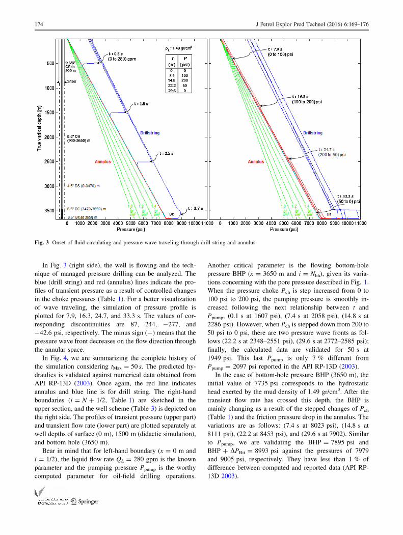
In Fig. 3 (right side), the well is flowing and the tech-

nique of managed pressure drilling can be analyzed. The

blue (drill string) and red (annulus) lines indicate the pro-

files of transient pressure as a result of controlled changes

in the choke pressures (Table 1). For a better visualization

of wave traveling, the simulation of pressure profile is

plotted for 7.9, 16.3, 24.7, and 33.3 s. The values of cor-

responding discontinuities are 87, 244, -277, and

-42.6 psi, respectively. The minus sign (-) means that the

pressure wave front decreases on the flow direction through

the annular space.

In Fig. 4, we are summarizing the complete history of

the simulation considering tMax ¼ 50 s. The predicted hy-

draulics is validated against numerical data obtained from

API RP-13D (2003). Once again, the red line indicates

annulus and blue line is for drill string. The right-hand

boundaries (i = N ? 1/2, Table 1) are sketched in the

upper section, and the well scheme (Table 3) is depicted on

the right side. The profiles of transient pressure (upper part)

and transient flow rate (lower part) are plotted separately at

well depths of surface (0 m), 1500 m (didactic simulation),

and bottom hole (3650 m).

Bear in mind that for left-hand boundary (x = 0 m and

i = 1/2), the liquid flow rate QL = 280 gpm is the known

parameter and the pumping pressure Ppump is the worthy

computed parameter for oil-field drilling operations.

Another critical parameter is the flowing bottom-hole

pressure BHP (x = 3650 m and i = Nbh), given its varia-

tions concerning with the pore pressure described in Fig. 1.

When the pressure choke Pch is step increased from 0 to

100 psi to 200 psi, the pumping pressure is smoothly in-

creased following the next relationship between t and

Ppump, (0.1 s at 1607 psi), (7.4 s at 2058 psi), (14.8 s at

2286 psi). However, when Pch is stepped down from 200 to

50 psi to 0 psi, there are two pressure wave fronts as fol-

lows (22.2 s at 2348–2551 psi), (29.6 s at 2772–2585 psi);

finally, the calculated data are validated for 50 s at

1949 psi. This last Ppump is only 7 % different from

Ppump = 2097 psi reported in the API RP-13D (2003).

In the case of bottom-hole pressure BHP (3650 m), the

initial value of 7735 psi corresponds to the hydrostatic

head exerted by the mud density of 1.49 gr/cm3. After the

transient flow rate has crossed this depth, the BHP is

mainly changing as a result of the stepped changes of Pch

(Table 1) and the friction pressure drop in the annulus. The

variations are as follows: (7.4 s at 8023 psi), (14.8 s at

8111 psi), (22.2 at 8453 psi), and (29.6 s at 7902). Similar

to Ppump, we are validating the BHP = 7895 psi and

BHP ? DPBit = 8993 psi against the pressures of 7979

and 9005 psi, respectively. They have less than 1 % of

difference between computed and reported data (API RP-

13D 2003).

Fig. 3 Onset of fluid circulating and pressure wave traveling through drill string and annulus


123

Special attention is focused on the profile of transient

flow rate QL, (lower part, Fig. 4). The left-hand boundary

(Eq. 3; Table 1), QL = 280 gpm remains constant for the

whole simulation. It is depicted by the blue line at 0 m.

However, in order to explain some slugging flow com-

monly observed at the surface end of the annular space, QL

at the right boundary (i = N ? 1/2) shall be discussed in

detail. First, at 7.4 s, QL is increased from 0 to 283 gpm,

and it is related to the time spent by the pressure wave

traveling along the oil well (Fig. 3). Next, at 14.8 s, there is

a sudden decrease from 254.6 to 52 gpm as Pch changes up

to 200 psi. The opposite transient effect is reflected when

Pch decreases to 50 psi at 22.2 s, then QL rises from 148 to

498.5 gpm. The oil well continues discharging at 29.6 s,

and the liquid flow rate slightly increases from 465 to

503 gpm. This ‘‘up-and-down’’ behavior of the oil-well

hydraulics is supported by the criteria of mass conserva-

tion. Moreover, all of these QL variations affect directly the

Fig. 4 History of simulation including profiles of transient pressure and transient liquid flow rate


123

transient values of friction pressure drop, DPBit and Ppump.

Finally, the simulating conditions are unaltered until 50 s

to converge to steady state defined by 280 gpm for all well

sections.

Conclusions

The Godunov scheme was applied for modeling transient

phenomena during actual oil-well drilling. The pressure

wave traveling along the well was described when the

managed pressure drilling is utilized. The set of initial and

boundary conditions can be consistently established with

the oil-well geometry and true operational conditions of the

drilling hydraulics. The numerical model based on the

finite-volume method was presented and solved using the

definition of the Riemann problem for the entire physical

domain and time length of simulation. The source term

must includes the effects of potential energy together with

energy dissipated by the friction mechanism. The simula-

tion was discussed in detail for the most important pa-

rameters: choke pressure, pumping pressure, bottom-hole

pressure, and circulating flow rate. As computed results are

close to reported oil-well data in API RP-13D (2003), the

Godunov scheme has high-potential engineering applica-

tions for modeling the transient drilling hydraulics, i.e.,

controlled flow, underbalanced drilling, and foam ce-

menting. Also, implementing high-order Godunov schemes

is suggested to improve the quality of computed results,

coupling with the heat transfer equations and the models of

fluid-rock interaction.

Acknowledgments The authors wish to state their appreciation to

Instituto Mexicano del Petroleo for their permission to publish this

article.

Open Access This article is distributed under the terms of the

Creative Commons Attribution 4.0 International License (http://

creativecommons.org/licenses/by/4.0/), which permits unrestricted

use, distribution, and reproduction in any medium, provided you give

appropriate credit to the original author(s) and the source, provide a

link to the Creative Commons license, and indicate if changes were

made.

References

API RP-13D (2003) Recommended practice on the rheology and

hydraulics of oil-well drilling fluids, 4th edn. American

Petroleum Institute, Washington

Bilgesu HI, Koperna GJ Jr (1995). The impact of friction factor on the

pressure loss prediction in gas pipelines. SPE30996, SPE Eastern

Regional Conference and Exhibition, Morgantown

Bousso S, Fuamba M (2013) Numerical simulation of unsteady

friction in transient two-phase flow with Godunov method.

J Water Resour Prot 5:1048–1058

Brkic D (2011) Review of explicit approximation to the Colebrook

relation for flow friction. J Petrol Sci Eng 77(1):34–48

Guinot V (2001) Numerical simulation of two-phase flow in pipes

using Godunov method. Int J Numer Meth Eng 50:1169–1189

Guinot V (2003) Godunov-type schemes: an introduction for engi-

neers, Chapter 5. Elsevier, Amsterdam

Kerger F, Archambeau P, Erpicum S, Dewals BJ, Pirotton M (2011)

An exact Riemann solver and a Godunov scheme for simulating

highly transient mixed flows. J Comput Appl Math

235:2030–2040

Nicolas-Lopez R, Valdiviezo-Mijangos OC, Valle-Molina C (2012)

New approach to calculate the mud density for wellbore stability

using the asymptotic homogenization theory. Pet Sci Technol

30(12):1239–1249

Toro EF (2009) Riemann solvers and numerical methods for fluid

dynamics. Springer, New York


123

Documents

Dynamic modeling of managed pressure drilling applying transient Godunov … · 2017-08-28 · engineering applications for modeling the transient drilling hydraulics, i.e., controlled