Dynamic Fund Protection

Elias S. W. Shiu

The University of Iowa

Iowa City

U.S.A.

Presentation based on two papers:

Hans U. Gerber and Gerard Pafumi, “Pricing Dynamic Investment Fund Protection,” North American Actuarial Journal, Vol 4 (2), 2000

Hans U. Gerber and Elias S.W. Shiu, “Pricing Perpetual Fund Protection with Withdrawal Protection,” North American Actuarial Journal, Vol 7 (2), 2003

Presentation based on two papers by Hans U. Gerber:

Hans U. Gerber and Gerard Pafumi, “Pricing Dynamic Investment Fund Protection,” North American Actuarial Journal, Vol 4 (2), 2000

Hans U. Gerber and Elias S.W. Shiu, “Pricing Perpetual Fund Protection with Withdrawal Protection,” North American Actuarial Journal, Vol 7 (2), 2003

Questions → hgerber@hec.unil.ch

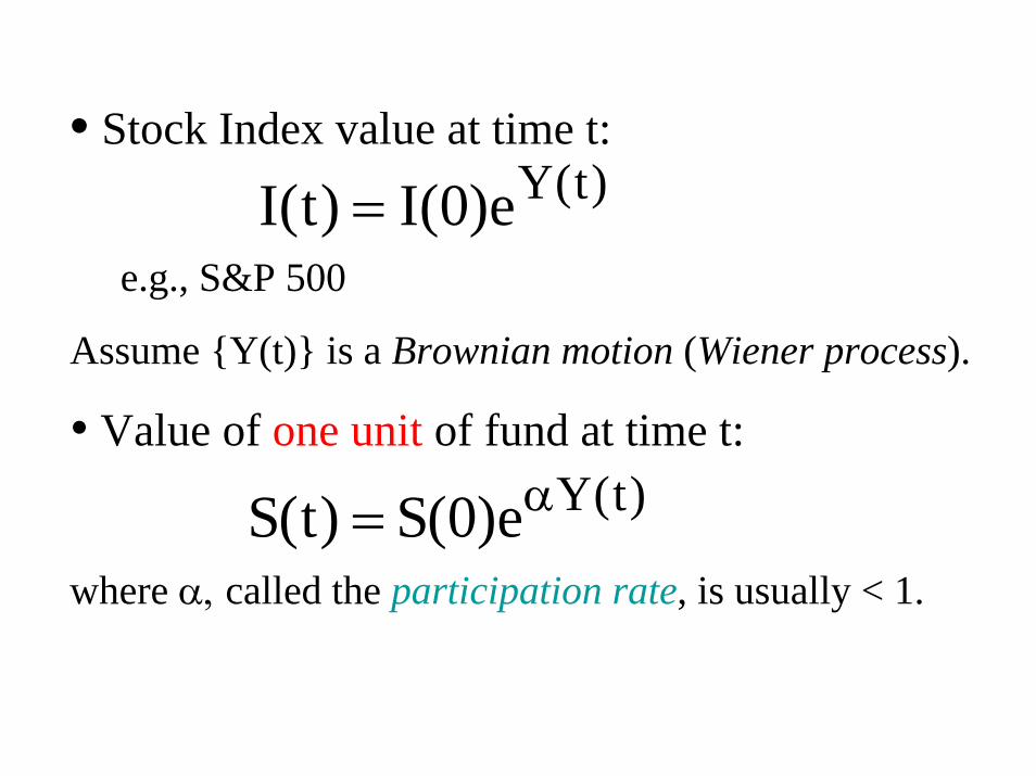
• Stock Index value at time t:

e.g., S&P 500

Assume {Y(t)} is a Brownian motion (Wiener process).

• Value of one unit of fund at time t:

where α, called the participation rate, is usually < 1.

)t(Ye)0(S)t(S α=

)t(Ye)0(I)t(I =

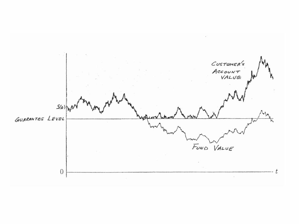
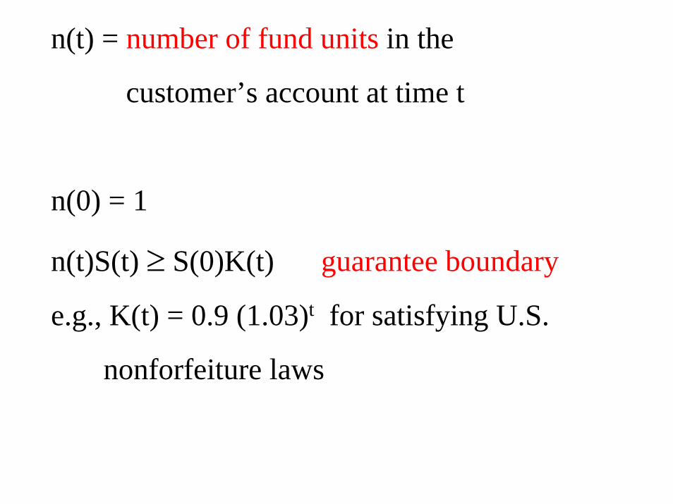
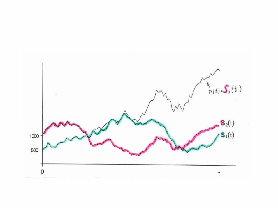
n(t) = number of fund units in the

customer’s account at time t

n(0) = 1

n(t)S(t) ≥ S(0)K(t) guarantee boundary

e.g., K(t) = 0.9 (1.03)t for satisfying U.S.

nonforfeiture laws

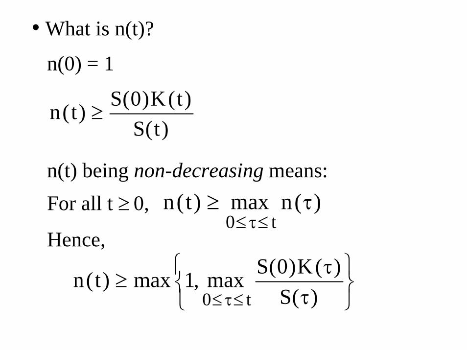
• What is n(t)?

n(0) = 1

n(t) being non-decreasing means:For all t ≥ 0,

Hence,

)t(S)t(K)0(S)t(n ≥

)(nmax)t(nt0

τ≥≤τ≤

⎭⎩ τ≤τ≤ )(St0⎬⎫

⎨⎧ τ

≥)(K)0(Smax,1max)t(n

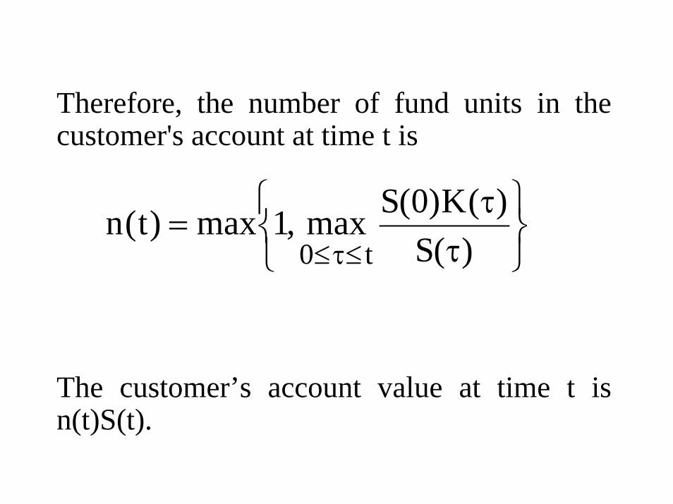
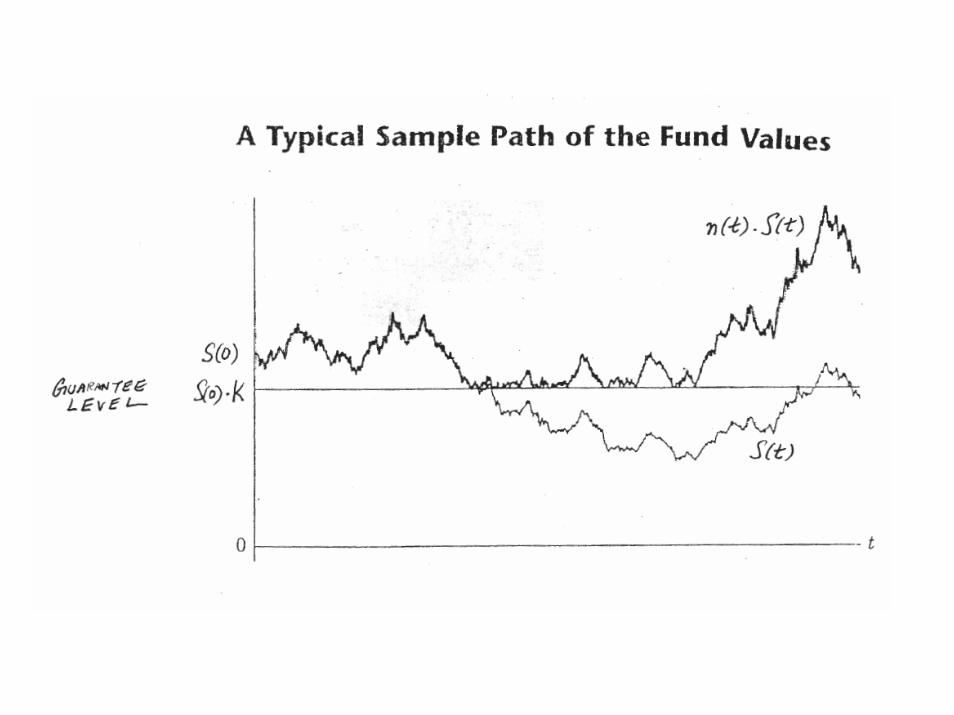
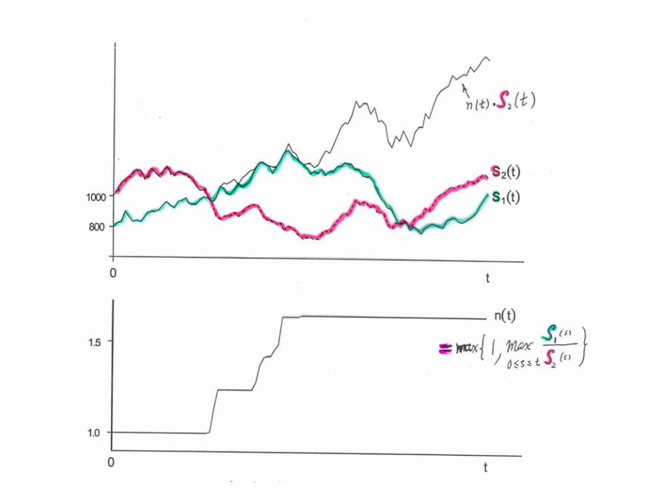
Therefore, the number of fund units in the customer's account at time t is

The customer’s account value at time t is n(t)S(t).

⎭⎬⎫

⎩⎨⎧

ττ

=≤τ≤ )(S

)(K)0(Smax,1max)t(nt0

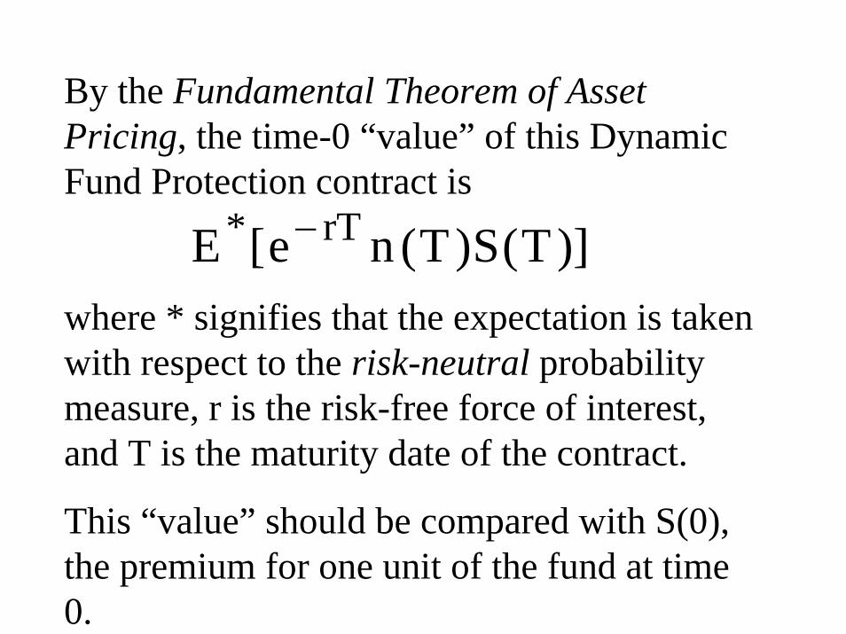
By the Fundamental Theorem of Asset Pricing, the time-0 “value” of this Dynamic Fund Protection contract is

where * signifies that the expectation is taken with respect to the risk-neutral probability measure, r is the risk-free force of interest, and T is the maturity date of the contract.

This “value” should be compared with S(0), the premium for one unit of the fund at time 0.

)]T(S)T(ne[E rT* −

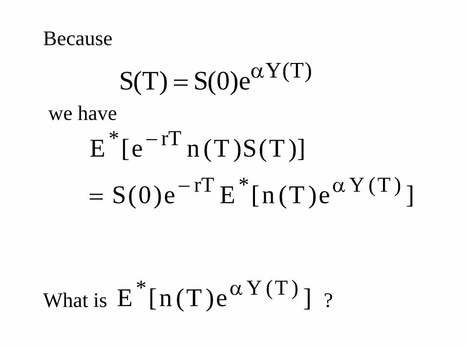
Because

we have

What is ?

)T(Ye)0(S)T(S α=

]e)T(n[Ee)0(S

)]T(S)T(ne[E)T(Y*rT

rT*

α−

−

=

]e)T(n[E )T(Y* α

]e[E )]T(n[E

]e[E]e[E

]e)T(n[E

]e)T(n[E

)T(Y***

)T(Y*)T(Y*

)T(Y*

)T(Y*

α

αα

α

α

=

=

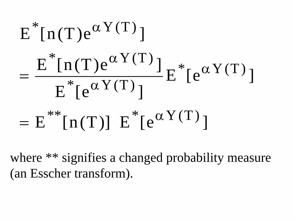
where ** signifies a changed probability measure (an Esscher transform).

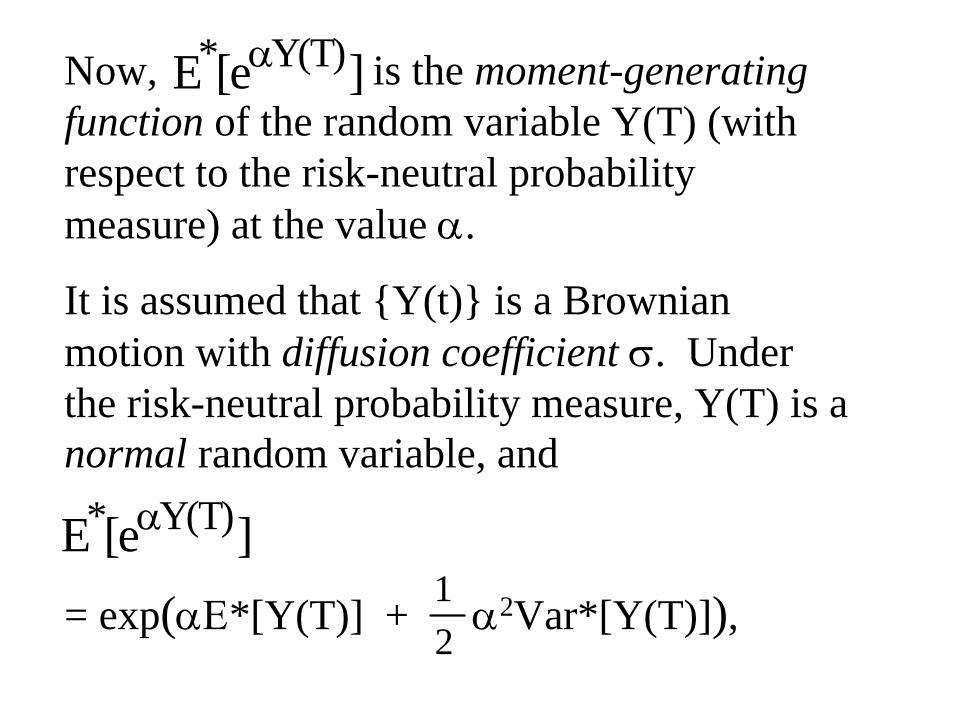
Now, is the moment-generating function of the random variable Y(T) (with respect to the risk-neutral probability measure) at the value α.

It is assumed that {Y(t)} is a Brownian motion with diffusion coefficient σ. Under the risk-neutral probability measure, Y(T) is a normal random variable, and

= exp(αΕ*[Y(T)] + α2Var*[Y(T)]),

]e[E )T(Y* α

21

]e[E )T(Y* α

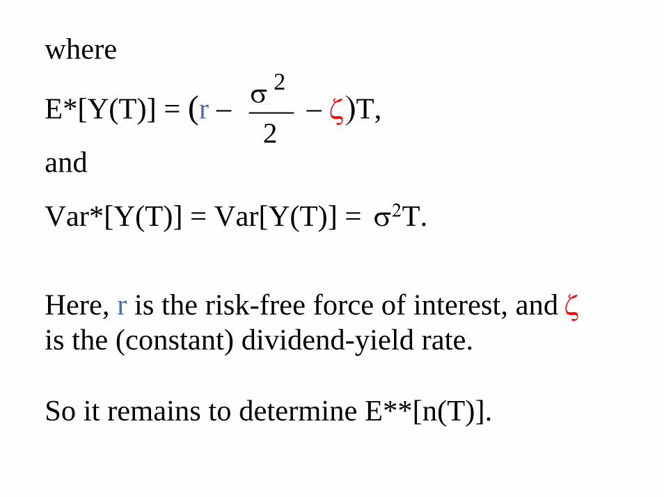
where

E*[Y(T)] = (r − − ζ)T,

and

Var*[Y(T)] = Var[Y(T)] = σ2T.

Here, r is the risk-free force of interest, and ζis the (constant) dividend-yield rate.

So it remains to determine E**[n(T)].

2

2σ

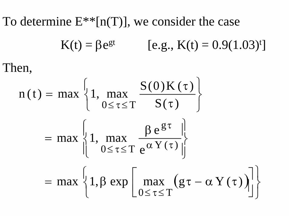
To determine E**[n(T)], we consider the case

K(t) = βegt [e.g., K(t) = 0.9(1.03)t]

Then,

( )⎭⎬⎫

⎩⎨⎧

⎥⎦⎤

⎢⎣⎡ τα−τβ=

⎪⎭

⎪⎬⎫

⎪⎩

⎪⎨⎧ β

=

⎭⎬⎫

⎩⎨⎧

ττ

=

≤τ≤

τα

τ

≤τ≤

≤τ≤

)(Ygmaxexp,1max

eemax,1max

)(S)(K)0(Smax,1max)t(n

T0

)(Y

g

T0

T0

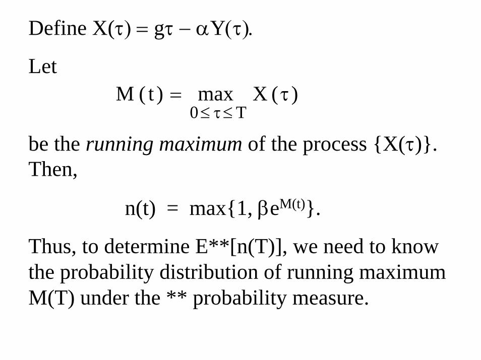
Define X(τ) = gτ − αY(τ).

Let

be the running maximum of the process {X(τ)}. Then,

n(t) = max{1, βeM(t)}.

Thus, to determine E**[n(T)], we need to know the probability distribution of running maximum M(T) under the ** probability measure.

)(Xmax)t(MT0

τ=≤τ≤

⎟⎠

⎞⎜⎝

⎛σ

µ−−Φ−

⎟⎠

⎞⎜⎝

⎛σ

µ−Φ=≤

σµ

ttme

ttm]m)t(MPr[

2/m2

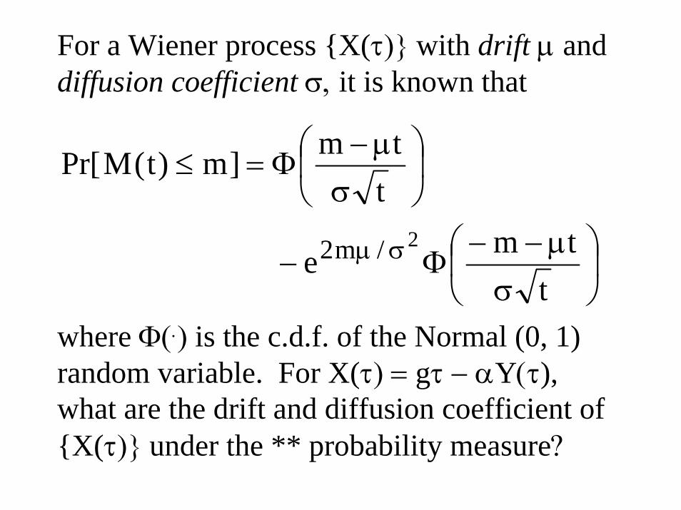
For a Wiener process {X(τ)} with drift µ and diffusion coefficient σ, it is known that

where Φ(.) is the c.d.f. of the Normal (0, 1) random variable. For X(τ) = gτ − αY(τ),what are the drift and diffusion coefficient of {X(τ)} under the ** probability measure?

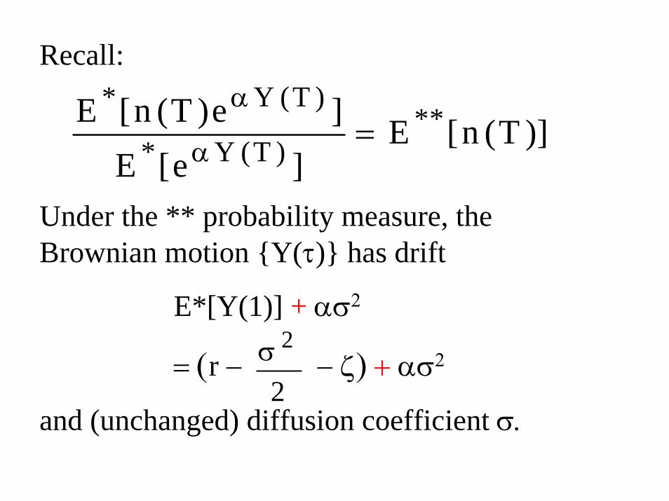
Recall:

Under the ** probability measure, the Brownian motion {Y(τ)} has drift

E*[Y(1)] + ασ2

= (r − − ζ) + ασ2

and (unchanged) diffusion coefficient σ.

)]T(n[E]e[E

]e)T(n[E **)T(Y*

)T(Y*=

α

α

2

2σ

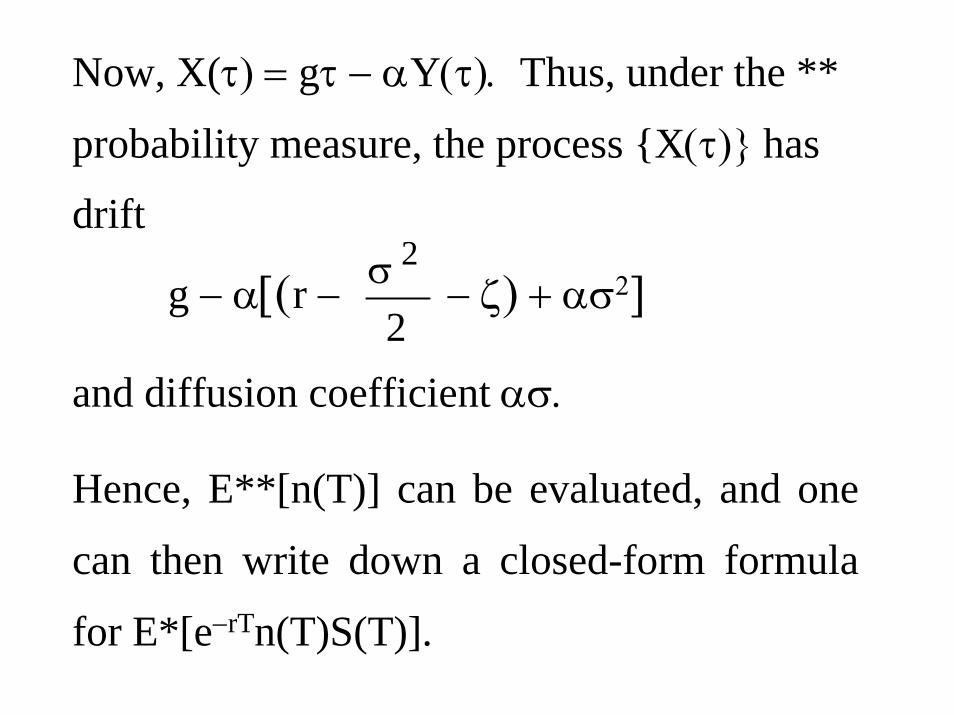
Now, X(τ) = gτ − αY(τ). Thus, under the **

probability measure, the process {X(τ)} has

drift

g − α[(r − − ζ) + ασ2]

and diffusion coefficient ασ.

Hence, E**[n(T)] can be evaluated, and one

can then write down a closed-form formula

for E*[e−rTn(T)S(T)].

2

2σ

Generalize to stochastic guarantee boundary:

⎥⎥⎦

⎤

⎢⎢⎣

⎡τ

⎭⎬⎫

⎩⎨⎧

ττ

≤τ≤

−∗ )(S)(S)(Smax,1maxeE 2

2

1T0

rT

⎥⎥⎦

⎤

⎢⎢⎣

⎡

⎭⎬⎫

⎩⎨⎧

ττ

≤τ≤

−∗ )T(S)(S

)(K)0(Smax,1maxeET0

rT

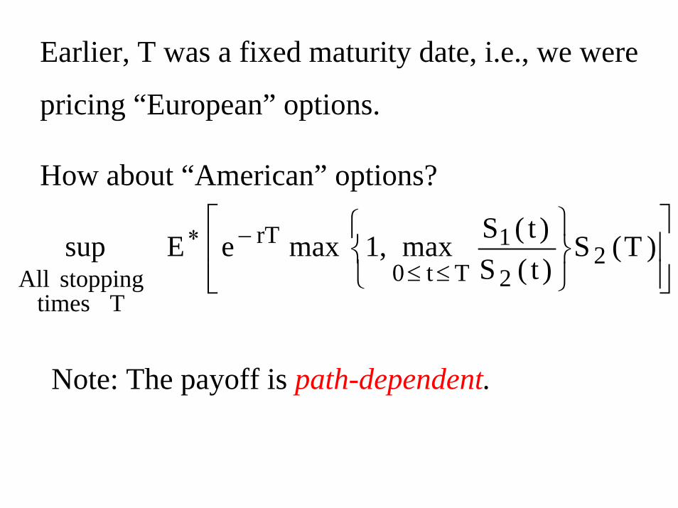
Note: The payoff is path-dependent.

⎥⎥⎦

⎤

⎢⎢⎣

⎡

⎭⎬⎫

⎩⎨⎧

≤≤

−∗ )T(S)t(S)t(Smax,1maxeEsup 2

2

1Tt0

rT

T timesstopping All

Earlier, T was a fixed maturity date, i.e., we were

pricing “European” options.

How about “American” options?

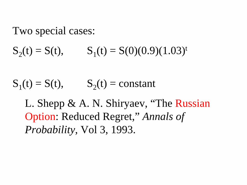
Two special cases:

S2(t) = S(t), S1(t) = S(0)(0.9)(1.03)t

S1(t) = S(t), S2(t) = constant

L. Shepp & A. N. Shiryaev, “The Russian Option: Reduced Regret,” Annals of Probability, Vol 3, 1993.

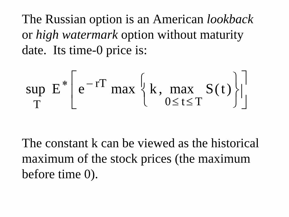
The Russian option is an American lookbackor high watermark option without maturity date. Its time-0 price is:

The constant k can be viewed as the historical maximum of the stock prices (the maximum before time 0).

⎥⎦

⎤⎢⎣

⎡

⎭⎬⎫

⎩⎨⎧

≤≤

−∗ )t(Smax,kmaxeEsupTt0

rT

T

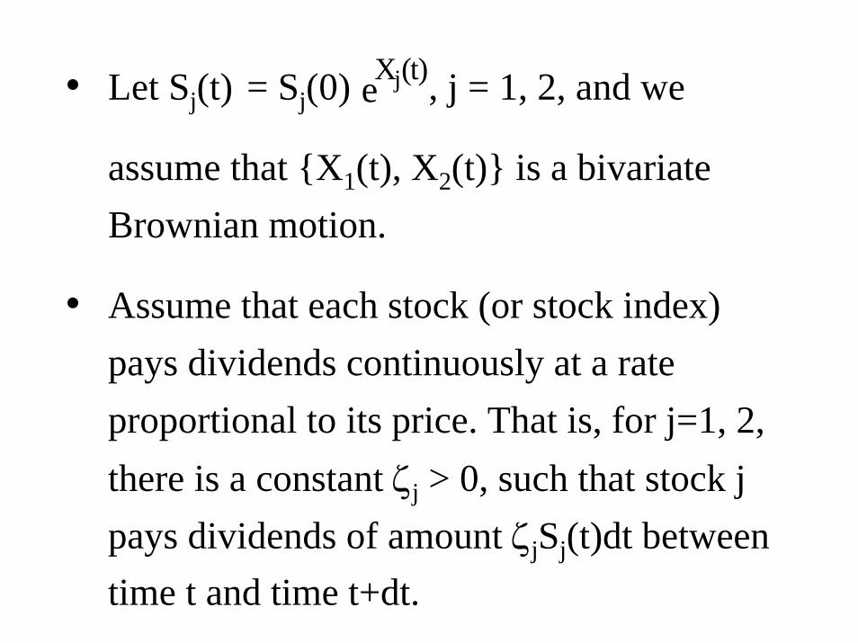
• Let Sj(t) = Sj(0) , j = 1, 2, and we

assume that {X1(t), X2(t)} is a bivariateBrownian motion.

• Assume that each stock (or stock index) pays dividends continuously at a rate proportional to its price. That is, for j=1, 2, there is a constant ζj > 0, such that stock j pays dividends of amount ζjSj(t)dt between time t and time t+dt.

)t(Xje

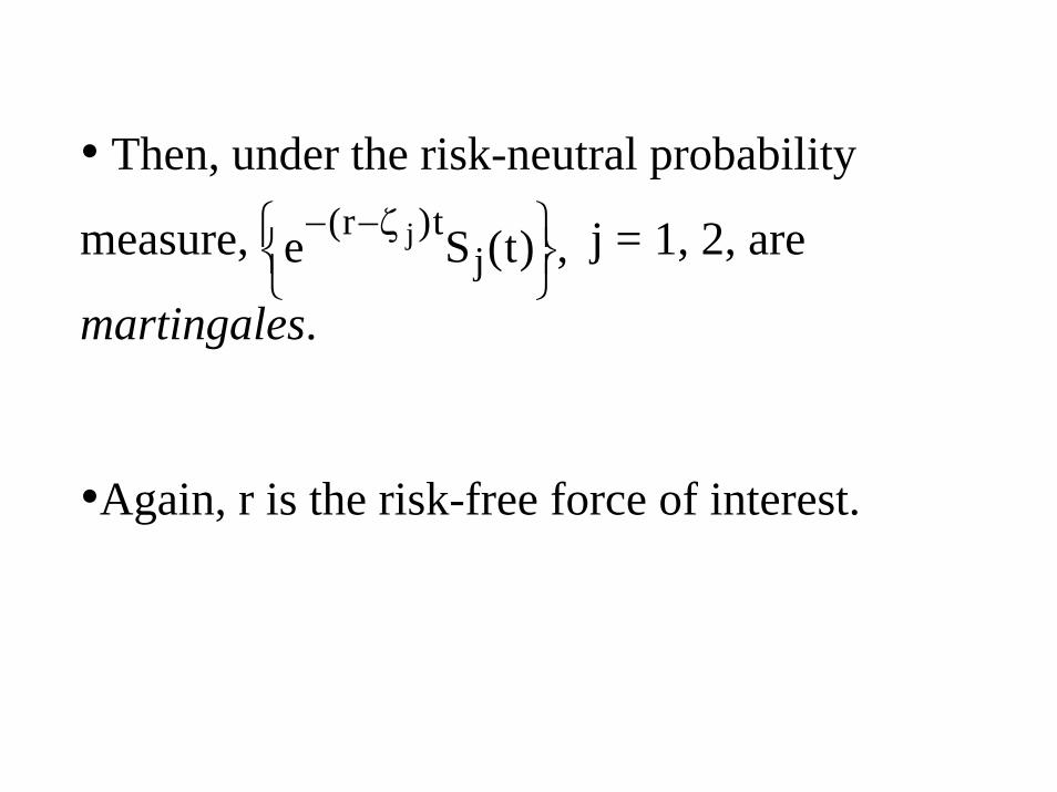
• Then, under the risk-neutral probability

measure, j = 1, 2, are

martingales.

•Again, r is the risk-free force of interest.

,)t(Se jt)r( j

⎭⎬⎫

⎩⎨⎧ ζ−−

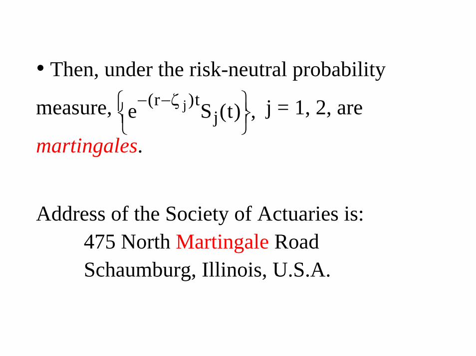
• Then, under the risk-neutral probability

measure, j = 1, 2, are

martingales.

Address of the Society of Actuaries is:475 North Martingale RoadSchaumburg, Illinois, U.S.A.

,)t(Se jt)r( j

⎭⎬⎫

⎩⎨⎧ ζ−−

•Address of the Institute of Actuaries of Australia is:

4 Martin Place, Sydney

But ….

•Address of the Institute of Actuaries of Australia is:

4 Martin Place, Sydney

But its current president is

Andrew Gale

•How about the Swiss Association of Actuaries?

•How about the Swiss Association of Actuaries?

Hans U. Gerber, “Martingales in Risk Theory,” Bulletin of the Swiss Association of Actuaries (1973), 205-216.

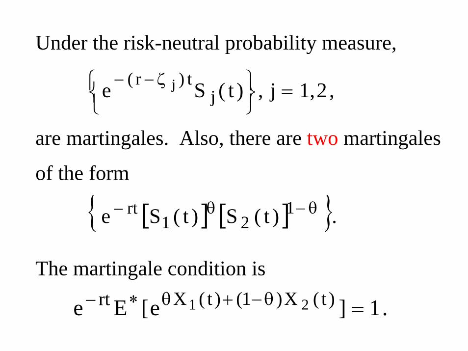
Under the risk-neutral probability measure,

are martingales. Also, there are two martingales

of the form

The martingale condition is

,2,1j,)t(Se jt)r( j =

⎭⎬⎫

⎩⎨⎧ ζ−−

[ ] [ ]{ }. )t(S)t(Se 121

rt θ−θ−

.1]e[Ee )t(X)1()t(Xrt 21 =θ−+θ∗−

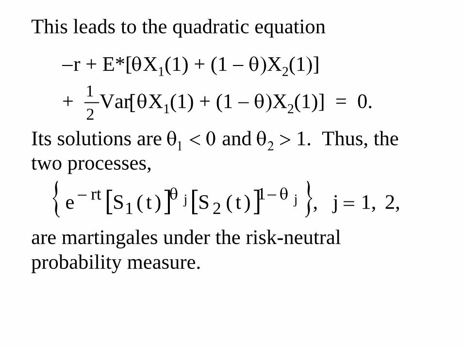
This leads to the quadratic equation

−r + E*[θX1(1) + (1 − θ)X2(1)]

+ Var[θX1(1) + (1 − θ)X2(1)] = 0.

Its solutions are θ1 < 0 and θ2 > 1. Thus, the two processes,

are martingales under the risk-neutral probability measure.

[ ] [ ]{ } 2, 1, j , )t(S)t(Se jj 121

rt =θ−θ−

21

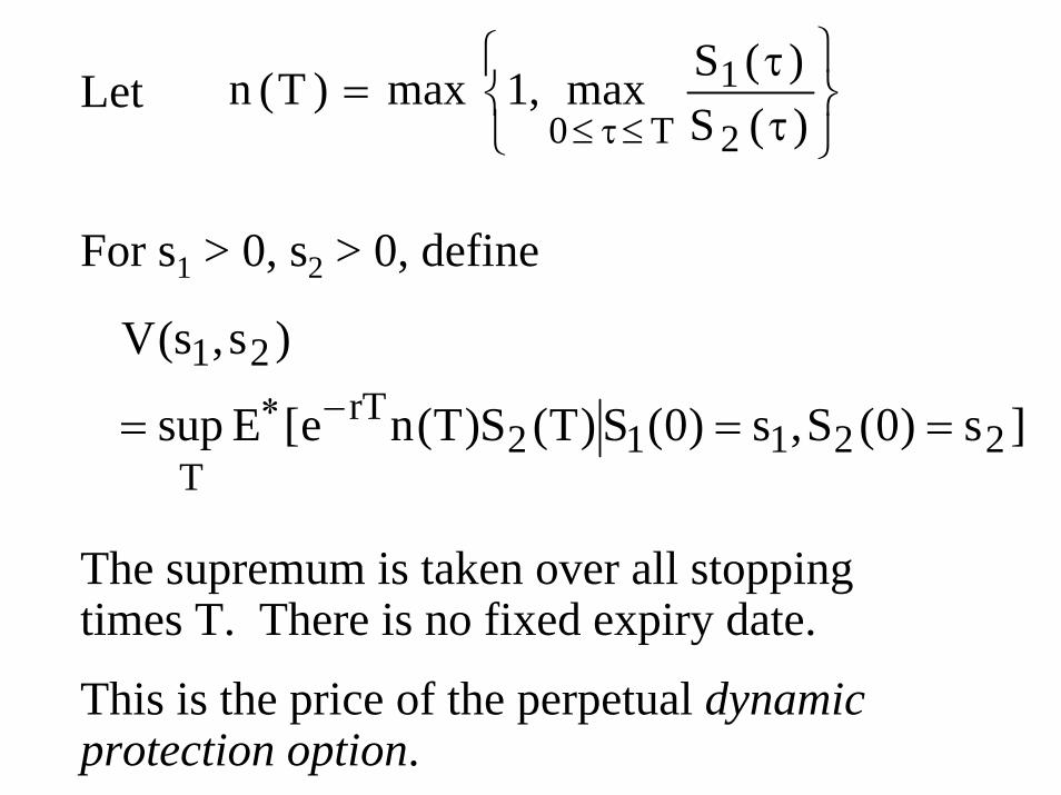
Let

For s1 > 0, s2 > 0, define

The supremum is taken over all stopping times T. There is no fixed expiry date.

This is the price of the perpetual dynamic protection option.

]s)0(S,s)0(S)T(S)T(ne[Esup

)s,s(V

22112rT

T

21

=== −∗

⎭⎬⎫

⎩⎨⎧

ττ

=≤τ≤ )(S

)(Smax,1max)T(n2

1T0

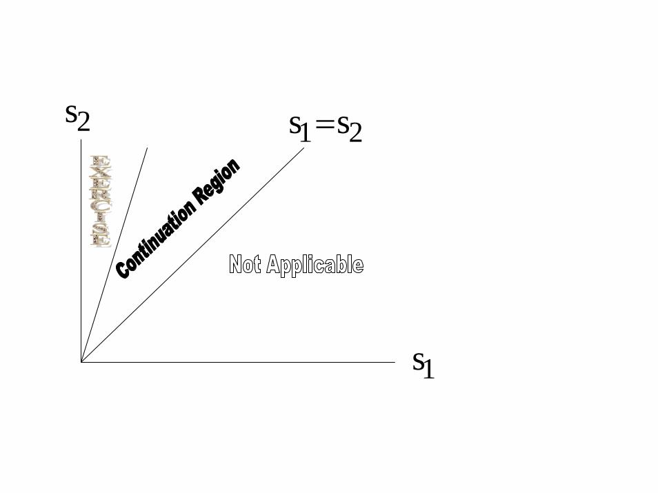
1s

21 ss =2s

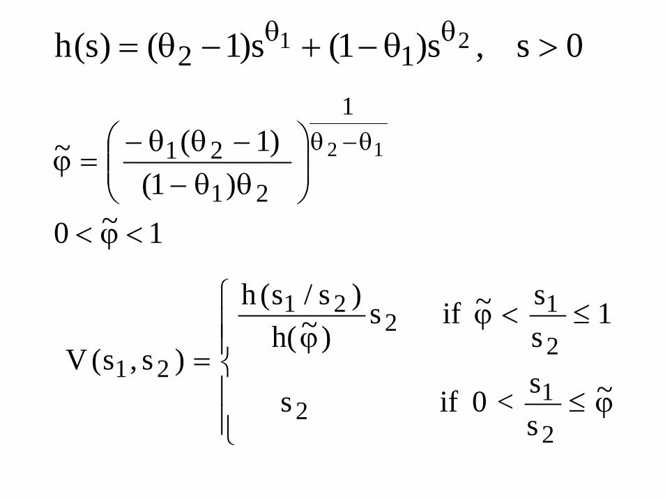
0s ,s)1(s)1()s(h 21 12 >θ−+−θ= θθ

1 ~ 0

) 1(

)1 (~ 12

1

21

21

<ϕ<

⎟⎟⎠

⎞⎜⎜⎝

⎛θθ−−θθ−

=ϕθ−θ

⎪⎪⎩

⎪⎪⎨

⎧

ϕ≤

≤<ϕϕ

=~

ss<0 if s

1ss~ if s

)~h()s/s(h

)s,s(V

2

12

2

12

21

21

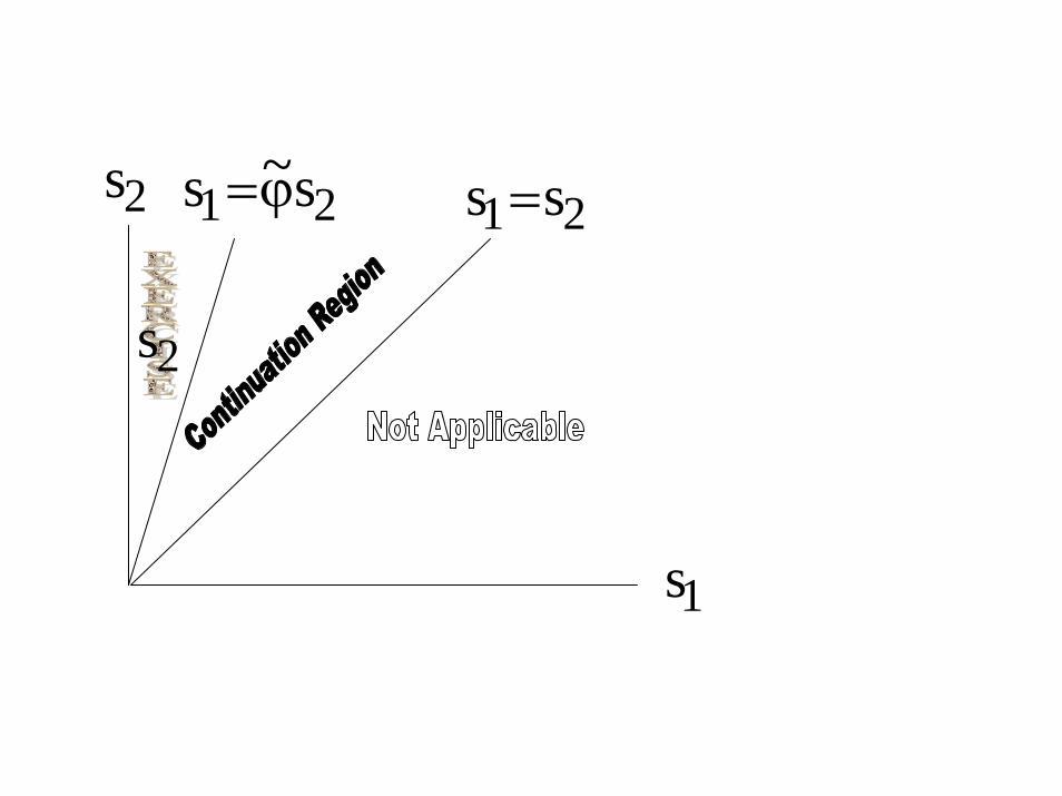
1s

21 ss =2s 21 s ~s ϕ=

2s

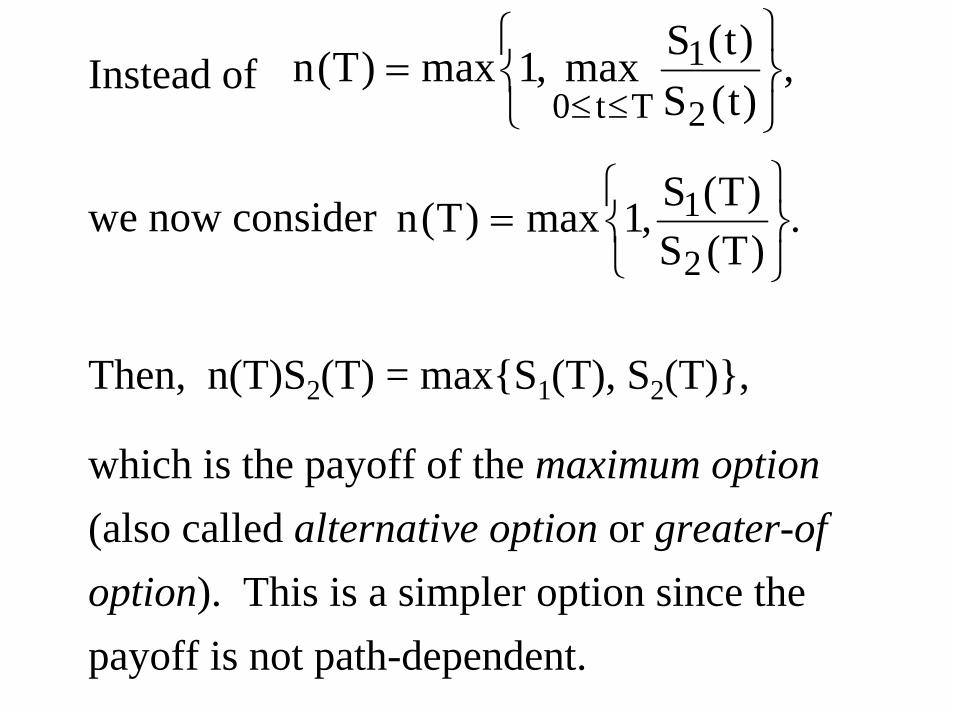
Instead of

we now consider

Then, n(T)S2(T) = max{S1(T), S2(T)},

which is the payoff of the maximum option (also called alternative option or greater-of option). This is a simpler option since the payoff is not path-dependent.

,)t(S)t(Smax,1max)T(n

2

1Tt0 ⎭

⎬⎫

⎩⎨⎧

=≤≤

.)T(S)T(S,1max)T(n

2

1

⎭⎬⎫

⎩⎨⎧

=

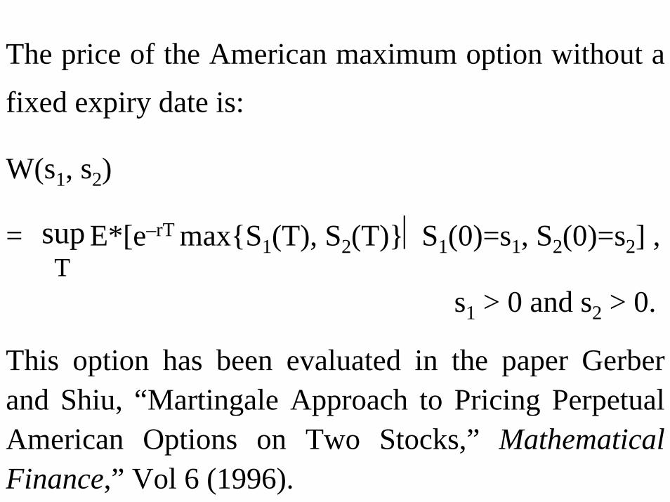
The price of the American maximum option without a fixed expiry date is:

W(s1, s2)

= E*[e–rT max{S1(T), S2(T)}⏐S1(0)=s1, S2(0)=s2] ,

s1 > 0 and s2 > 0.

This option has been evaluated in the paper Gerber and Shiu, “Martingale Approach to Pricing Perpetual American Options on Two Stocks,” Mathematical Finance,” Vol 6 (1996).

Tsup

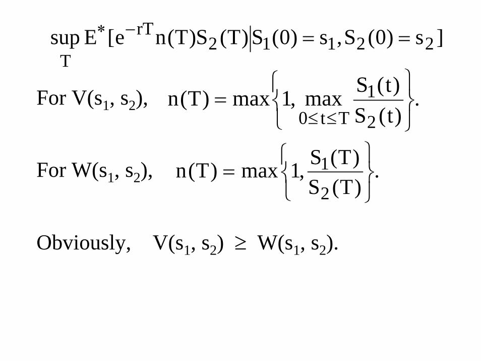
For V(s1, s2),

For W(s1, s2),

Obviously, V(s1, s2) ≥ W(s1, s2).

]s)0(S,s)0(S)T(S)T(ne[Esup 22112rT

T==−∗

.)t(S)t(Smax,1max)T(n

2

1Tt0 ⎭

⎬⎫

⎩⎨⎧

=≤≤

.)T(S)T(S,1max)T(n

2

1

⎭⎬⎫

⎩⎨⎧

=

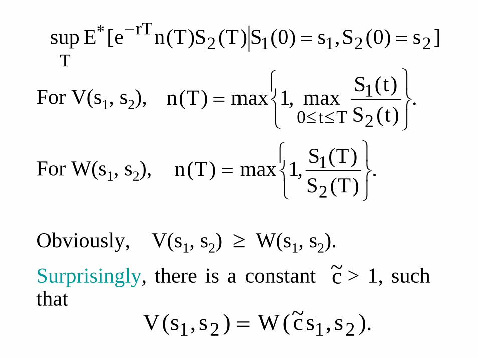
For V(s1, s2),

For W(s1, s2),

Obviously, V(s1, s2) ≥ W(s1, s2).

Surprisingly, there is a constant > 1, such that

]s)0(S,s)0(S)T(S)T(ne[Esup 22112rT

T==−∗

.)t(S)t(Smax,1max)T(n

2

1Tt0 ⎭

⎬⎫

⎩⎨⎧

=≤≤

.)T(S)T(S,1max)T(n

2

1

⎭⎬⎫

⎩⎨⎧

=

c~

).s,sc~(W)s,s(V 2121 =

1s

2s

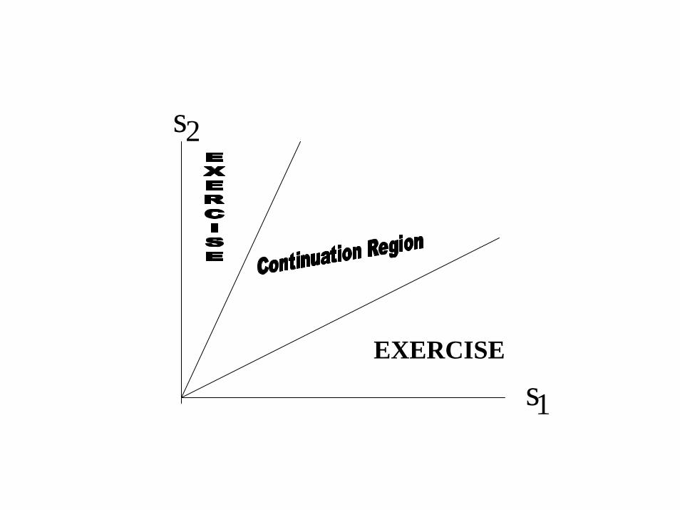
EXERCISE

)/()1(

2

2)/()1(

1

1122121

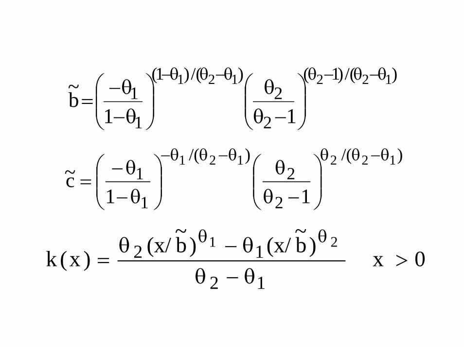
11b~

θ−θ−θθ−θθ−

⎟⎟⎠

⎞⎜⎜⎝

⎛−θ

θ⎟⎟⎠

⎞⎜⎜⎝

⎛θ−θ−

=

)/(

2

2)/(

1

1122121

11c~

θ−θθθ−θθ−

⎟⎟⎠

⎞⎜⎜⎝

⎛−θ

θ⎟⎟⎠

⎞⎜⎜⎝

⎛θ−θ−

=

0 x )b~(x/)b~(x/)x(k12

12 21>

θ−θθ−θ

=θθ

⎪⎪⎪

⎩

⎪⎪⎪

⎨

⎧

≥

<<

≤

=

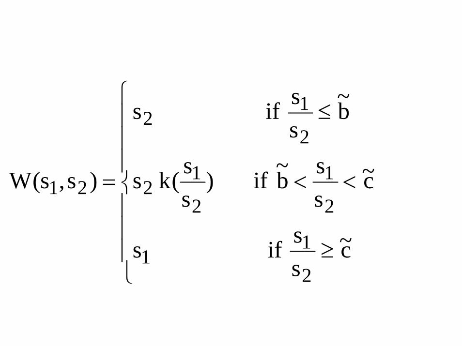
c~ss if s

c~ssb~ if )

ss(ks

b~ss if s

)s,s(W

2

11

2

1

2

1 2

2

12

21

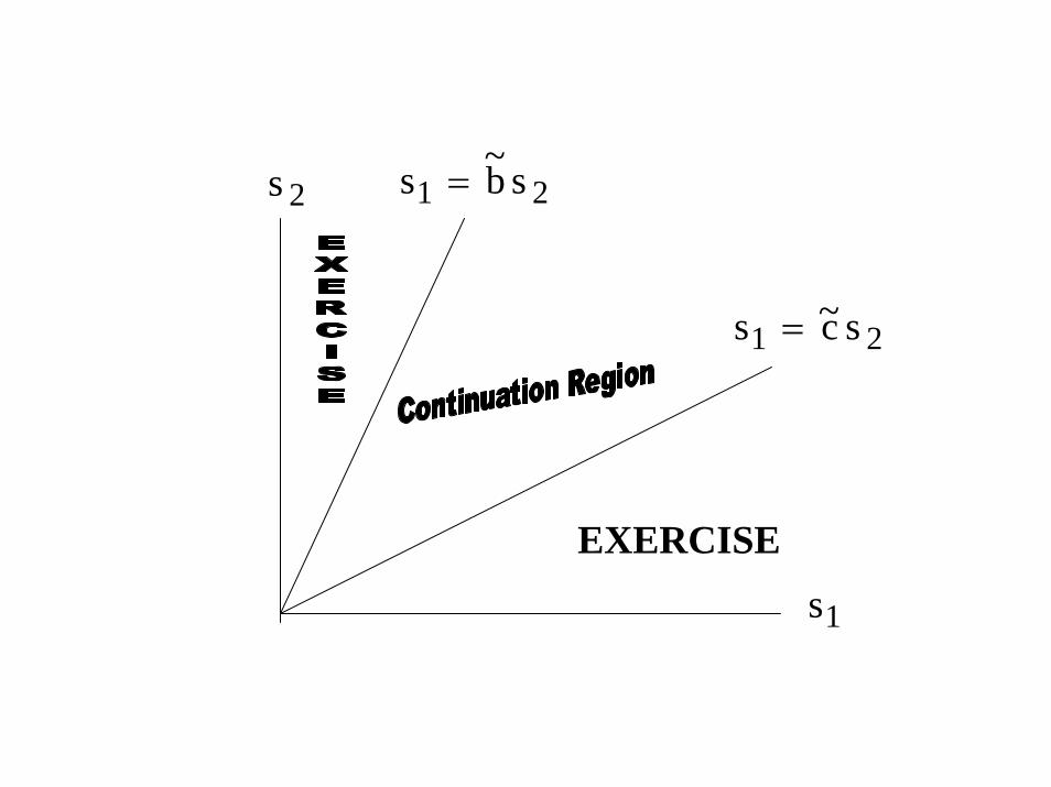
EXERCISE

21 sc~ s =

21 sb~ s =2s

1s

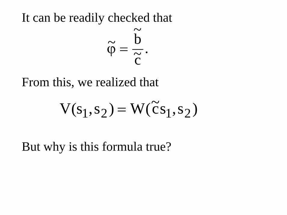
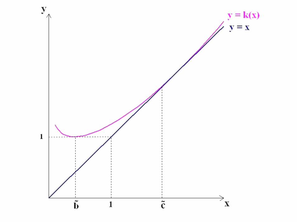
It can be readily checked that

From this, we realized that

But why is this formula true?

.c~b~~ =ϕ

)s,sc~(W)s,s(V 2121 =

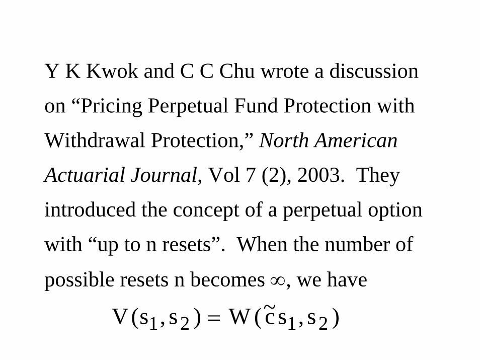
Y K Kwok and C C Chu wrote a discussion on “Pricing Perpetual Fund Protection with Withdrawal Protection,” North American Actuarial Journal, Vol 7 (2), 2003. They introduced the concept of a perpetual option with “up to n resets”. When the number of

possible resets n becomes ∞, we have

)s,sc~(W)s,s(V 2121 =

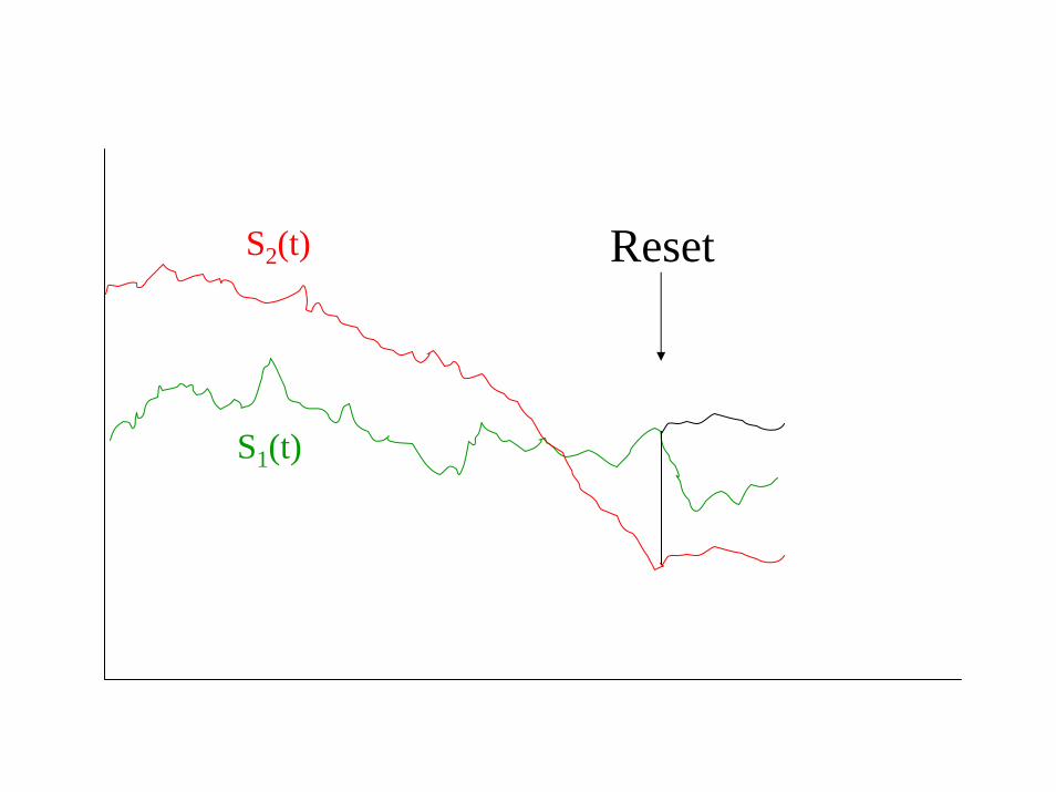
S1(t)

S2(t) Reset

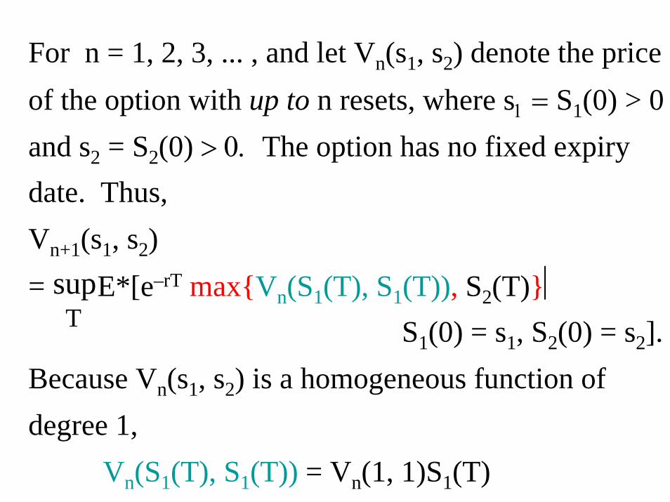
For n = 1, 2, 3, ... , and let Vn(s1, s2) denote the price of the option with up to n resets, where s1 = S1(0) > 0 and s2 = S2(0) > 0. The option has no fixed expiry date. Thus,Vn+1(s1, s2)= E*[e–rT max{Vn(S1(T), S1(T)), S2(T)}⏐

S1(0) = s1, S2(0) = s2].Because Vn(s1, s2) is a homogeneous function of degree 1,

Vn(S1(T), S1(T)) = Vn(1, 1)S1(T)

Tsup

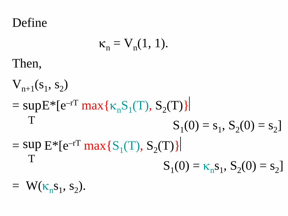
Define κn = Vn(1, 1).

Then,Vn+1(s1, s2)

= E*[e–rT max{κnS1(T), S2(T)}⏐

S1(0) = s1, S2(0) = s2]= E*[e–rT max{S1(T), S2(T)}⏐

S1(0) = κns1, S2(0) = s2]= W(κns1, s2).

Tsup

Tsup

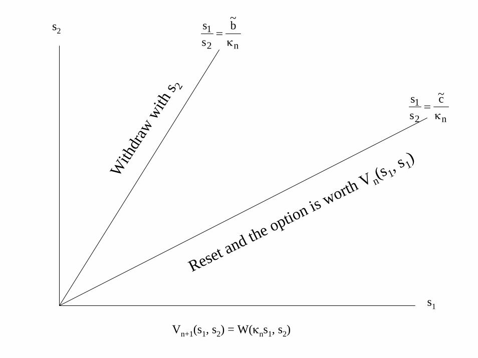
s2

s1

n2

1 b~

ss

κ=

n2

1 c~

ss

κ=

With

draw

with

s 2

Reset and the option is worth V n(s 1, s 1)

Vn+1(s1, s2) = W(κns1, s2)

Vn+1(s1, s2) = W(κns1, s2)

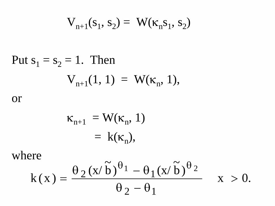
Put s1 = s2 = 1. ThenVn+1(1, 1) = W(κn, 1),

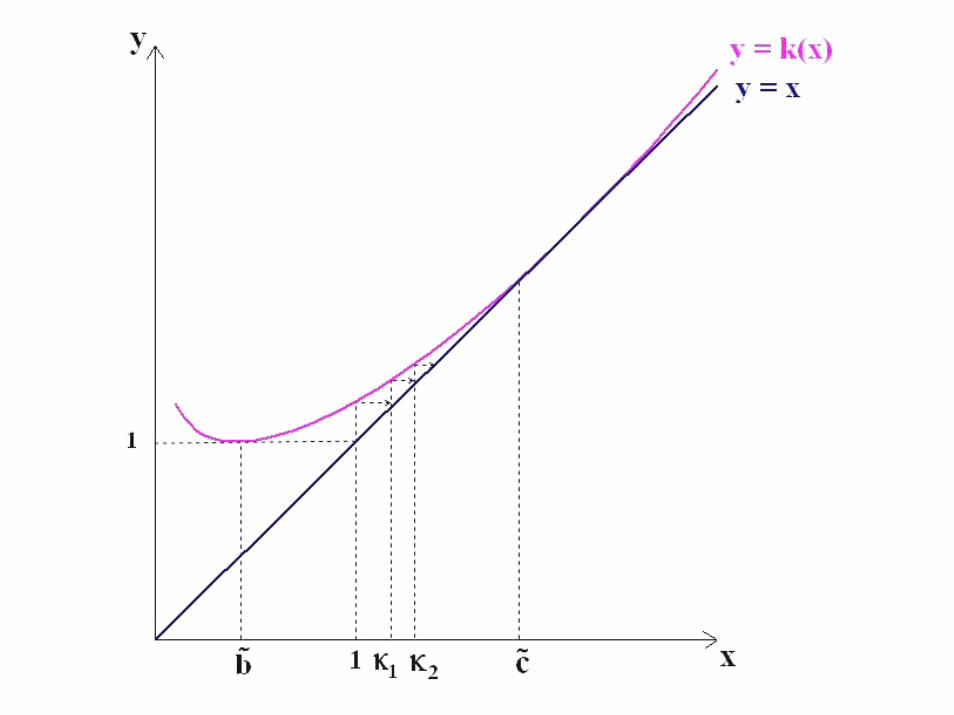
orκn+1 = W(κn, 1)

= k(κn),where

0. x )b~(x/)b~(x/)x(k12

12 21>

θ−θθ−θ

=θθ

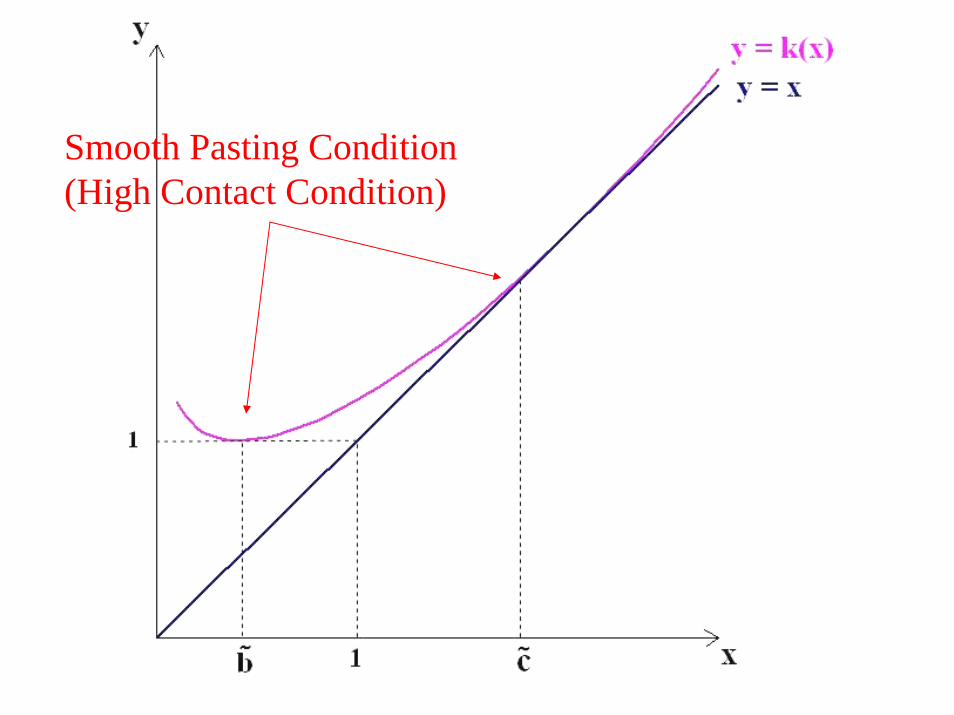
Smooth Pasting Condition(High Contact Condition)

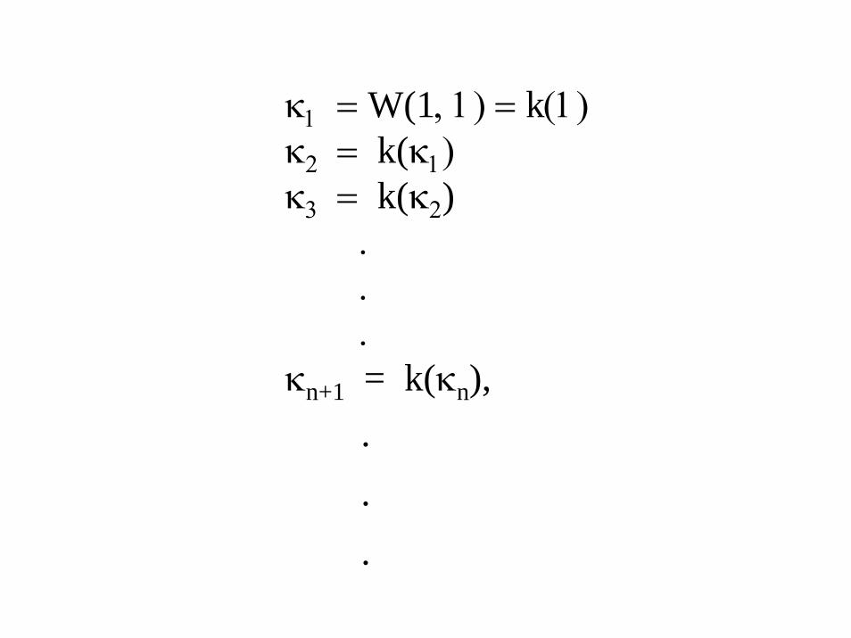
κ1 = W(1, 1) = k(1)κ2 = k(κ1)κ3 = k(κ2)

.

.

.κn+1 = k(κn),

.

.

.

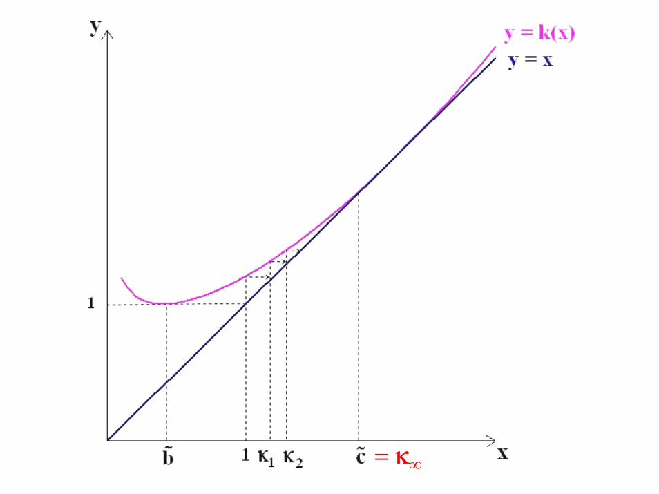
= κ∞

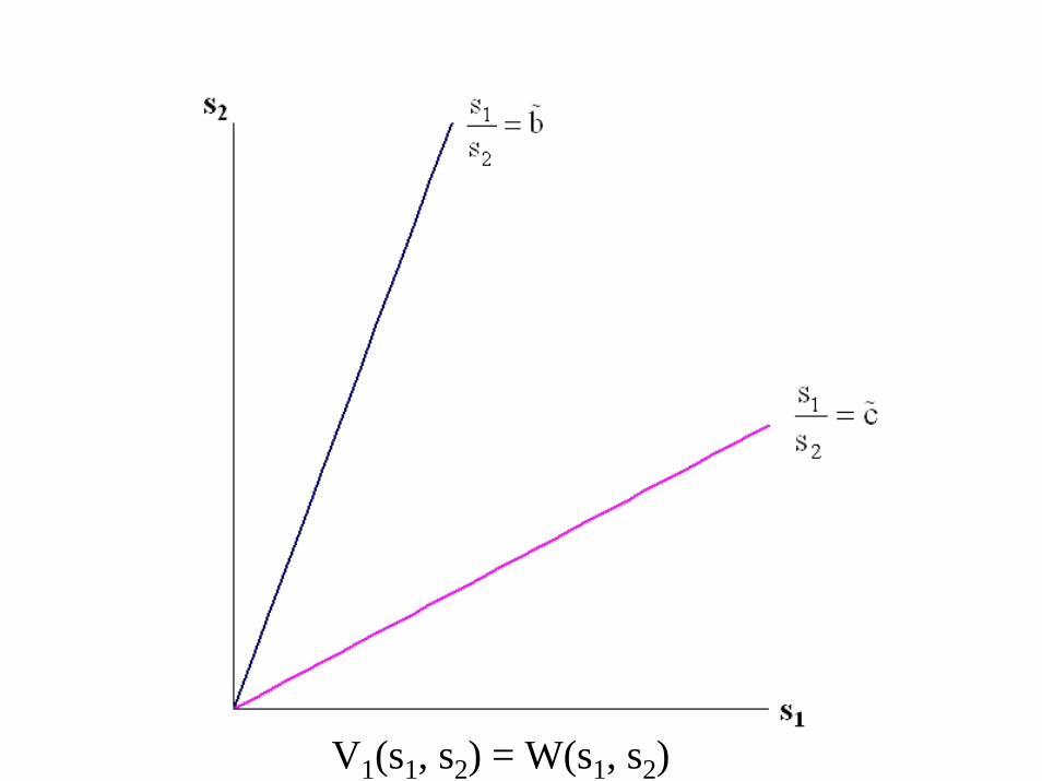
V1(s1, s2) = W(s1, s2)

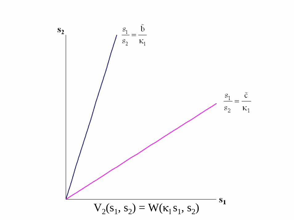
V2(s1, s2) = W(κ1s1, s2)

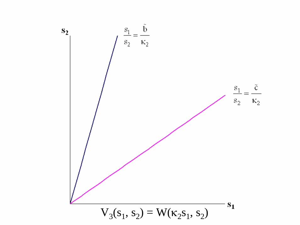
V3(s1, s2) = W(κ2s1, s2)

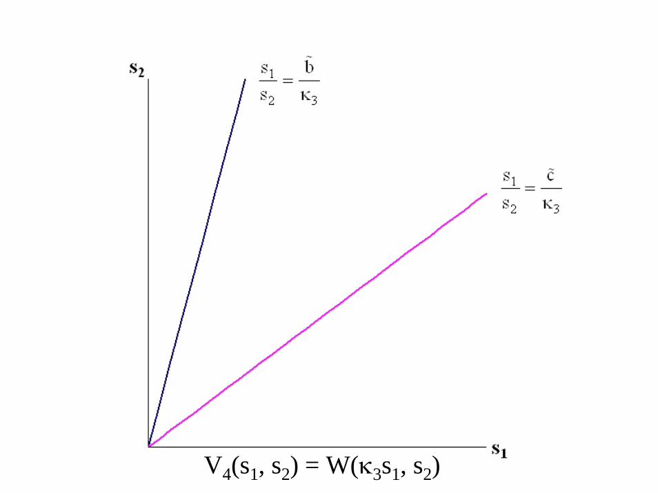
V4(s1, s2) = W(κ3s1, s2)

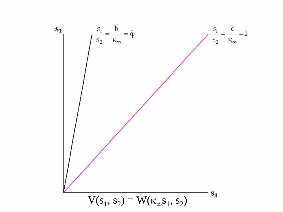
V(s1, s2) = W(κ∞s1, s2)

H. U. Gerber and G. Pafumi, “Pricing Dynamic Investment Fund Protection,” North American Actuarial Journal, Vol 4 (2), 2000.

J. Imai and P. P. Boyle, “Dynamic Fund Protection,” North American Actuarial Journal, Vol 5 (3), 2001.

H. U. Gerber and E. S.W. Shiu, “Pricing Perpetual Fund Protection with Withdrawal Protection,” North American Actuarial Journal, Vol 7 (2), 2003.

H,-K. Fung and L. K. Li, “Pricing Discrete Dynamic Fund Protection,” North American Actuarial Journal, Vol 7 (4), 2003.

C. C. Chu and Y. K. Kwok, “Reset and Withdrawal Rights in Dynamic Fund Protection,” Insurance: Mathematics and Economics, Vol 34, 2004.

H. U. Gerber and G. Pafumi, “Pricing Dynamic Investment Fund Protection,” North American Actuarial Journal, Vol 4 (2), 2000.

J. Imai and P. P. Boyle, “Dynamic Fund Protection,” North American Actuarial Journal, Vol 5 (3), 2001.

H. U. Gerber and E. S.W. Shiu, “Pricing Perpetual Fund Protection with Withdrawal Protection,” North American Actuarial Journal, Vol 7 (2), 2003.

H,-K. Fung and L. K. Li, “Pricing Discrete Dynamic Fund Protection,” North American Actuarial Journal, Vol 7 (4), 2003.

C. C. Chu and Y. K. Kwok, “Reset and Withdrawal Rights in Dynamic Fund Protection,” Insurance: Mathematics and Economics, Vol 34, 2004.

Thank you for your patience

Time for lunch