University of LjubljanaFaculty of Mathematics and Physics

Department of Physics

Seminar - 4th year

Dynamic Fragmentation of Bodies at Different Scales

Author: Jure Beričič

Adviser: prof. doc. dr. Simon Širca

Ljubljana, April 2011

Abstract

This seminar is focused on dynamic fragmentation. It starts by showing differences between Mott and Schuhmann plot, two widely used plots in studies of fragmentation. This is followed by a deriv-ation of the fragment size distribution for a homogeneous fragmentation of an infinite continuous thin body. This concept is then extended and supporting examples are provided. Following this is a method for determining the scale factor of the fragment size distribution based on energy prin-ciples. Last chapter is trying to answer the question of why spaghetti does not break in half.

Index

1. Dynamic fragmentation.................................................................................................................12. Data Representation....................................................................................................................12.1. Mott plot....................................................................................................................................12.2. Schuhmann plot........................................................................................................................23. Fragment size distribution............................................................................................................23.1. Homogeneous fragmentation of an infinite continuous thin body...............................................23.2. Extension...................................................................................................................................33.3. Examples...................................................................................................................................54. Determining the scale factor.........................................................................................................65. Spaghetti fragmentation...............................................................................................................76. Conclusion...................................................................................................................................97. References.................................................................................................................................11

i

1. Dynamic fragmentation

Dynamic fragmentation [1] is identified with both the process and the out-come of an event in which a monolithic structure or body is subjected to intense and abrupt interior or exterior forces causing it to break up into a number of component parts (fragments). It covers a large number of different events that span over many length scales. The processes ranging from high energy colli-sion of nuclei, through explosion of shells, to fragmentation of the Shoemaker-Levy comet and even to the distribution and fabric of galaxies and galactic clusters can be thought of as examples of dynamic fragmentation. A more common example is the impact of a wine glass on kitchen floor. Fragmentation is strongly dependent on locality of effect that causes fragmentation, but in this work we will focus on phenomenological description.

Many applications are interested in product of dynamic fragmentation: the size distribution, the ve-locities and the governing length size of the fragments. But the final state of the fragmentation is closely related to the fracture process, which strongly depends on the material (liquid, ductile metal or brittle solid) and energetic conditions in the experiment.

In this seminar I will present one way to obtain size distribution and the governing length size of the fragments in case of an extreme energy fragmentation of non-brittle materials. In the end I will show why spaghetti breaks into more than two pieces, which is a completely different example of fragmentation.

2. Data Representation

In any fragmentation event we get numerous fragments of different sizes and masses. We need some sort of representation of this data. There are two widely known plots that can be used to dis-play the nature of the fragmentation: the Mott plot and the Schuhmann plot.

2.1. Mott plot

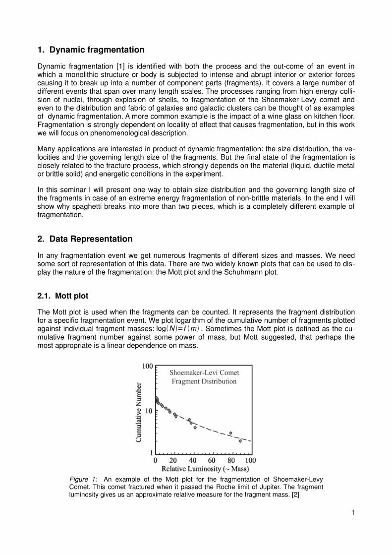
The Mott plot is used when the fragments can be counted. It represents the fragment distribution for a specific fragmentation event. We plot logarithm of the cumulative number of fragments plotted against individual fragment masses: log(N)=f (m) . Sometimes the Mott plot is defined as the cu-mulative fragment number against some power of mass, but Mott suggested, that perhaps the most appropriate is a linear dependence on mass.

Figure 1: An example of the Mott plot for the fragmentation of Shoemaker-Levy Comet. This comet fractured when it passed the Roche limit of Jupiter. The fragment luminosity gives us an approximate relative measure for the fragment mass. [2]

1

2.2. Schuhmann plot

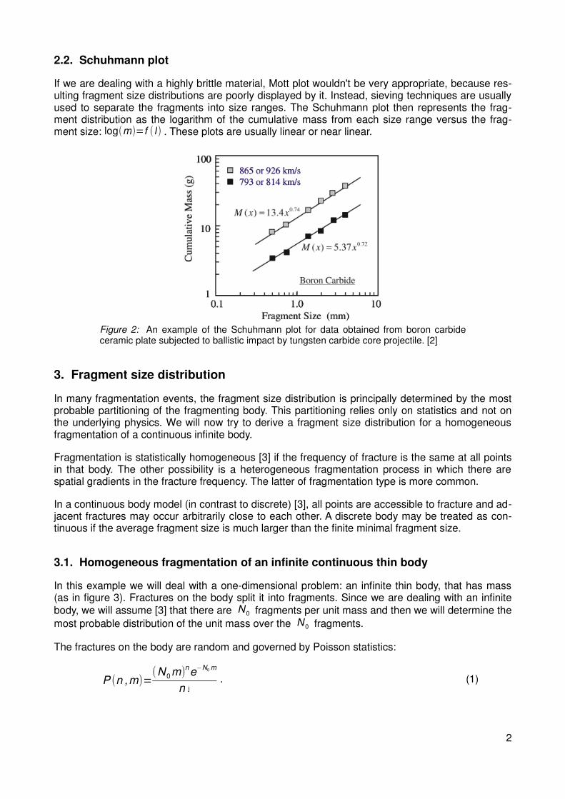
If we are dealing with a highly brittle material, Mott plot wouldn't be very appropriate, because res-ulting fragment size distributions are poorly displayed by it. Instead, sieving techniques are usually used to separate the fragments into size ranges. The Schuhmann plot then represents the frag-ment distribution as the logarithm of the cumulative mass from each size range versus the frag-ment size: log(m)=f ( l ) . These plots are usually linear or near linear.

Figure 2: An example of the Schuhmann plot for data obtained from boron carbide ceramic plate subjected to ballistic impact by tungsten carbide core projectile. [2]

3. Fragment size distribution

In many fragmentation events, the fragment size distribution is principally determined by the most probable partitioning of the fragmenting body. This partitioning relies only on statistics and not on the underlying physics. We will now try to derive a fragment size distribution for a homogeneous fragmentation of a continuous infinite body.

Fragmentation is statistically homogeneous [3] if the frequency of fracture is the same at all points in that body. The other possibility is a heterogeneous fragmentation process in which there are spatial gradients in the fracture frequency. The latter of fragmentation type is more common.

In a continuous body model (in contrast to discrete) [3], all points are accessible to fracture and ad-jacent fractures may occur arbitrarily close to each other. A discrete body may be treated as con-tinuous if the average fragment size is much larger than the finite minimal fragment size.

3.1. Homogeneous fragmentation of an infinite continuous thin body

In this example we will deal with a one-dimensional problem: an infinite thin body, that has mass (as in figure 3). Fractures on the body split it into fragments. Since we are dealing with an infinite

body, we will assume [3] that there are N 0 fragments per unit mass and then we will determine the

most probable distribution of the unit mass over the N 0 fragments.

The fractures on the body are random and governed by Poisson statistics:

P (n ,m)=(N0m)n

e−N0 m

n !. (1)

2

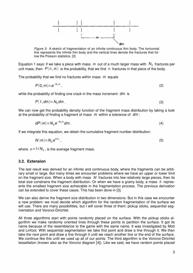
Figure 3: A sketch of fragmentation of an infinite continuous thin body. The horizontal line represents the infinite thin body and the vertical lines denote the fractures that fol-low the Poisson statistics. [3]

Equation 1 says: if we take a piece with mass m out of a much larger mass with N0 fractures per

unit mass, then P (n ,m) is the probability, that we find n fractures in that piece of the body.

The probability that we find no fractures within mass m equals

P (0,m )=e−N 0m , (2)

while the probability of finding one crack in the mass increment dm is

P (1,dm)=N0dm . (3)

We can now get the probability density function of the fragment mass distribution by taking a look at the probability of finding a fragment of mass m within a tolerance of dm :

dP (m)=N0e−N 0m

dm . (4)

If we integrate this equation, we obtain the cumulative fragment number distribution:

N (m)=N0em /μ

, (5)

where μ=1/N0 , is the average fragment mass.

3.2. Extension

The last result was derived for an infinite and continuous body, where the fragments can be arbit-rary small or large. But many times we encounter problems where we have an upper or lower limit on the fragment size. When a body with mass M fractures into few relatively large pieces, then its total size constrains the fragment distribution. Or when we have a grainy body, a mass δ repres-ents the smallest fragment size achievable in the fragmentation process. The previous derivation can be extended to cover these cases. This has been done in [3].

We can also derive the fragment size distribution in two dimensions. But in this case we encounter a new problem: we must decide which algorithm for the random fragmentation of the surface we will use. There are many possibilities, but I will cover three of them: pickup sticks, sequential seg-mentation and Voronoi-Dirichlet.

All three algorithms start with points randomly placed on the surface. With the pickup sticks al-gorithm we make randomly oriented lines through these points to partition the surface. It got its name because of the resemblance to the game with the same name. It was investigated by Mott and Linfoot. With sequential segmentation we take first point and draw a line through it. We then take the next point and draw a line through it until we reach another line or the end of the surface. We continue like this until we used up all of our points. The third algorithm is the Voronoi-Dirichlet tessellation (known also as the Voronoi diagram [4]). Like we said, we have random points placed

3

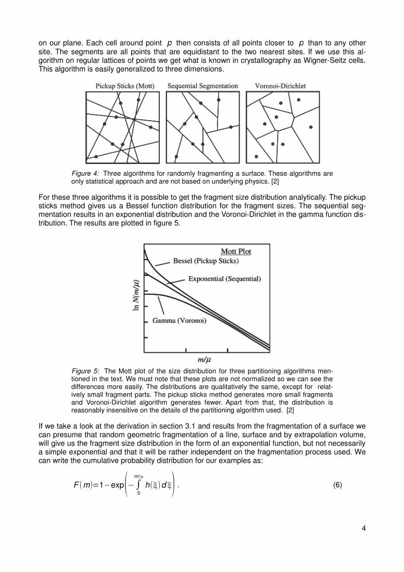
on our plane. Each cell around point p then consists of all points closer to p than to any other site. The segments are all points that are equidistant to the two nearest sites. If we use this al-gorithm on regular lattices of points we get what is known in crystallography as Wigner-Seitz cells. This algorithm is easily generalized to three dimensions.

Figure 4: Three algorithms for randomly fragmenting a surface. These algorithms are only statistical approach and are not based on underlying physics. [2]

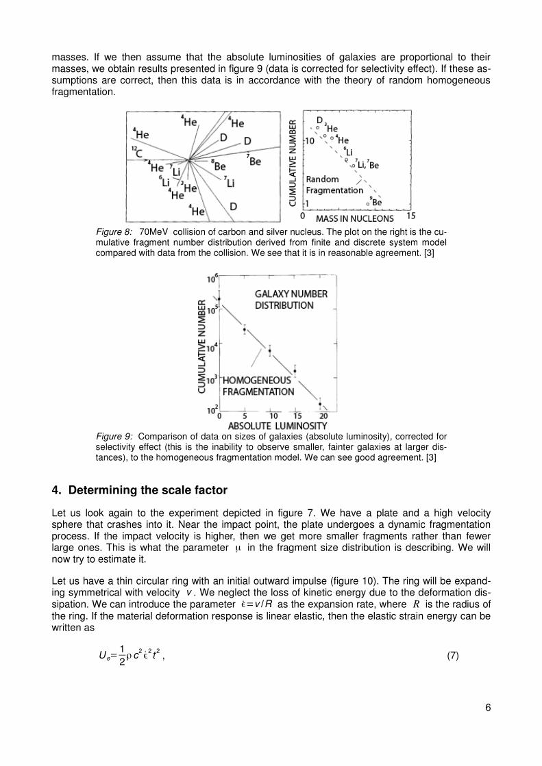
For these three algorithms it is possible to get the fragment size distribution analytically. The pickup sticks method gives us a Bessel function distribution for the fragment sizes. The sequential seg-mentation results in an exponential distribution and the Voronoi-Dirichlet in the gamma function dis-tribution. The results are plotted in figure 5.

Figure 5: The Mott plot of the size distribution for three partitioning algorithms men-tioned in the text. We must note that these plots are not normalized so we can see the differences more easily. The distributions are qualitatively the same, except for relat-ively small fragment parts. The pickup sticks method generates more small fragments and Voronoi-Dirichlet algorithm generates fewer. Apart from that, the distribution is reasonably insensitive on the details of the partitioning algorithm used. [2]

If we take a look at the derivation in section 3.1 and results from the fragmentation of a surface we can presume that random geometric fragmentation of a line, surface and by extrapolation volume, will give us the fragment size distribution in the form of an exponential function, but not necessarily a simple exponential and that it will be rather independent on the fragmentation process used. We can write the cumulative probability distribution for our examples as:

F (m)=1−exp(−∫0

m /μ

h(ξ)d ξ) . (6)

4

Here h(ξ) is the likelihood function and it varies from case to case. It is important that we have

only one parameter for our distribution: the size scale μ .

3.3. Examples

Historically important was the fragmentation of exploding ammunition. The most significant in this area is the work of Sir Nevill F. Mott during the last years of World War II. He tried to theoretically describe statistical fragmentation of ammunition subjected to intense explosive loading. Most of his efforts were to describe the breakup of explosively driven expanding cylindrical shells. Figure 6 shows the Mott plots for an explosive fragmentation of an AerMet-100 steel cylinder, which is rep-resentative for his work.

Figure 6: These pictures are from explosive fragmentation of AerMet-100 steel cylin-der. We see that distribution is in form of equation 6. [2]

Another ballistic example comes from the impact of a copper sphere onto a stainless steel plate (figure 7).

Figure 7: Impact of a copper sphere onto a stainless steel plate with two Mott plots for two tests with different impact velocities and angles (measured from the normal). Test 12: 60° and 3.26km /s ; test 13: 50° and 3.09km /s . [2]

A totally different case of dynamic fragmentation comes from the microscopic world, namely from 70MeV collision of carbon and silver nuclei. The collision results in 16 electrically charged frag-ments ranging from deuterium to beryllium. This was compared with a theoretical model for a finite and discrete system and it is in reasonable agreement (figure 8).

Yet another example is many length scales away from the carbon silver collision: the size distribu-tion of galaxies. Brown and his coworkers made a hypothesis that the universe was fragmented only once during the early stage after the Big Bang and was then separated into protogalactic

5

masses. If we then assume that the absolute luminosities of galaxies are proportional to their masses, we obtain results presented in figure 9 (data is corrected for selectivity effect). If these as-sumptions are correct, then this data is in accordance with the theory of random homogeneous fragmentation.

Figure 8: 70MeV collision of carbon and silver nucleus. The plot on the right is the cu-mulative fragment number distribution derived from finite and discrete system model compared with data from the collision. We see that it is in reasonable agreement. [3]

Figure 9: Comparison of data on sizes of galaxies (absolute luminosity), corrected for selectivity effect (this is the inability to observe smaller, fainter galaxies at larger dis-tances), to the homogeneous fragmentation model. We can see good agreement. [3]

4. Determining the scale factor

Let us look again to the experiment depicted in figure 7. We have a plate and a high velocity sphere that crashes into it. Near the impact point, the plate undergoes a dynamic fragmentation process. If the impact velocity is higher, then we get more smaller fragments rather than fewer large ones. This is what the parameter μ in the fragment size distribution is describing. We will now try to estimate it.

Let us have a thin circular ring with an initial outward impulse (figure 10). The ring will be expand-ing symmetrical with velocity v . We neglect the loss of kinetic energy due to the deformation dis-sipation. We can introduce the parameter ϵ̇=v /R as the expansion rate, where R is the radius of the ring. If the material deformation response is linear elastic, then the elastic strain energy can be written as

U e=1

2ρc

2ϵ̇

2t

2, (7)

6

where ρ is the density and c the elastic wave speed. [2]

Figure 10: A thin ring with an initial outward impulse. Equilibrium fragmentation is pos-sible when strain energy equals fracture energy. This occurs at the correlation distance λ which constrains the exponential fragment size distribution with one free parameter.

Equilibrium fragmentation is a term used in energy based fragmentation theory and refers to the ability of a body to undergo fragmentation when a specific theoretical en-ergy criterion is reached. If a material needs an additional failure criterion we talk about non-equilibrium fragmentation. [2]

There is another key quantity we must consider here. A region of the material within which the ma-terial points are within an elastic communication distance at any given time t is called the correla-tion horizon [2] and it is determined by the elastic wave speed c . Within the correlation horizon the elastic stresses can adjust to modest variations in the elastic modulus and concentrate stresses at points of weakness. The theory says that if the fragmentation occurs within time t , the fragments can not be larger than the region defined by the correlation horizon c t . With this information we can determine the boundary fracture surface energy as [2]

U s=3 Γc t . (8)

This is the amount of energy that needs to be provided from the increasing elastic strain energy so that fragmentation can occur (see figure 10). The numerical factor depends on whether we have an expanding ring, sphere or volume (the value 3 corresponds to expanding volume). If we are deal-

ing with a metal body with fracture toughness K c , then we can estimate the fracture surface en-

ergy by Γ≃K c

2/2ρc2

. From equations 7 and 8 we can get the expression for the scale factor:

λ≃(48 Γ

ρ ϵ̇2 )1/3

. (9)

Now it is possible to calculate the governing size directly from the material properties and strain rate measure of the intensity of the fragmentation process. The comparison of results from the ex-periment depicted in figure 7 with what we get from equation 9 for that case gives us a pretty good

agreement. The prediction for distribution with a measured value of μex=0.87g is μth=1.29g .

It needs to be said that the kinetic energy of the expanding ring in not included in the energy fuel-ing fragmentation. The kinetic energy for the expansion of the elastic ring is small ( ~15% ) com-pared to the elastic strain energy and because of that is disregarded.

7

5. Spaghetti fragmentation

Most spaghetti (if held at both ends and then bent over some critical curvature) will not break in half but in three or more pieces. We will now take a look at this phenomenon that also puzzled Feynman. We will be dealing with simplified model, where we will disregard some effects, such as shock-waves and details of plasticity and elasticity. It has to be noted that this problem is not a case of dynamic fragmentation, but a quasi-statically fragmentation. Here a body is broken when it experiences very small velocity.

Our problem is as follows: we have a thin rod held at both ends. We then start to slowly (quasistat-

ic) bend this rod so that its curvature is uniform. At time t=0 its initial curvature κ0 reaches the

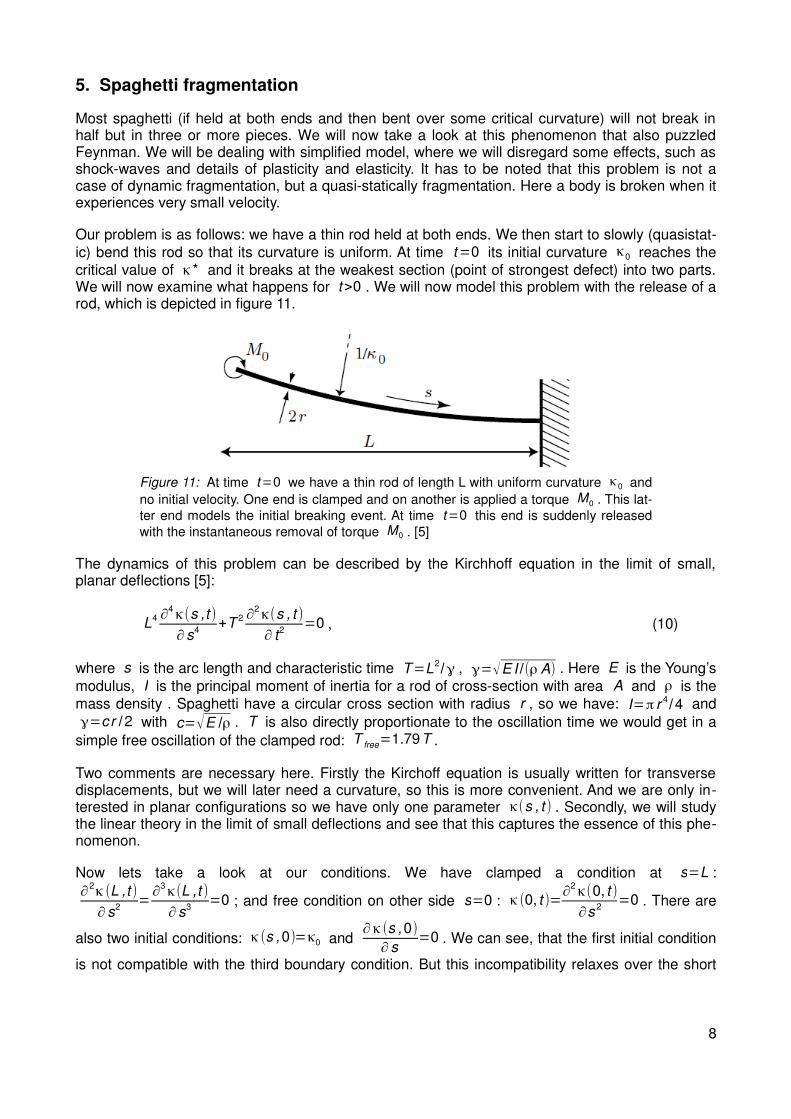
critical value of κ * and it breaks at the weakest section (point of strongest defect) into two parts. We will now examine what happens for t>0 . We will now model this problem with the release of a rod, which is depicted in figure 11.

Figure 11: At time t=0 we have a thin rod of length L with uniform curvature κ0 and

no initial velocity. One end is clamped and on another is applied a torque M0 . This lat-

ter end models the initial breaking event. At time t=0 this end is suddenly released

with the instantaneous removal of torque M0 . [5]

The dynamics of this problem can be described by the Kirchhoff equation in the limit of small, planar deflections [5]:

L4 ∂4 κ(s ,t )

∂s4+T 2 ∂2 κ(s , t )

∂ t2=0 , (10)

where s is the arc length and characteristic time T=L2/ γ , γ=√E I /(ρ A) . Here E is the Young’s

modulus, I is the principal moment of inertia for a rod of cross-section with area A and ρ is the

mass density . Spaghetti have a circular cross section with radius r , so we have: I=π r4/4 and

γ=cr /2 with c=√E /ρ . T is also directly proportionate to the oscillation time we would get in a

simple free oscillation of the clamped rod: T free=1.79T .

Two comments are necessary here. Firstly the Kirchoff equation is usually written for transverse displacements, but we will later need a curvature, so this is more convenient. And we are only in-terested in planar configurations so we have only one parameter κ(s , t ) . Secondly, we will study the linear theory in the limit of small deflections and see that this captures the essence of this phe-nomenon.

Now lets take a look at our conditions. We have clamped a condition at s=L :

∂2κ (L ,t )

∂s2=

∂3 κ(L ,t )

∂s3=0 ; and free condition on other side s=0 : κ(0, t )=

∂2 κ(0, t )

∂s 2=0 . There are

also two initial conditions: κ(s , 0)=κ0 and ∂κ(s ,0)

∂s=0 . We can see, that the first initial condition

is not compatible with the third boundary condition. But this incompatibility relaxes over the short

8

time scale T s ( T /T s∼104 [5]). This relaxation sends flexural waves which, as we will see later,

can break the rod.

Equation 10 can be solved analytically in the so-called intermediate asymptote regime: T s≪t≪T

. We get a solution that does not describe a progressive wave, s∼c t , but a self-similar solution

s∼√(γ t ) [5]:

κ(s , t )=2κ0S( 1

√2 πs

√γ t ) , (11)

with the Fresnel sine integral

S(x )=∫0

x

sin( π2

y2)dy . (12)

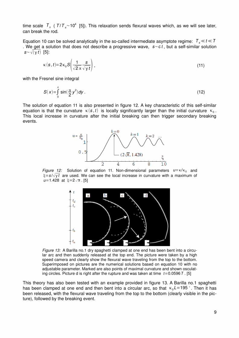
The solution of equation 11 is also presented in figure 12. A key characteristic of this self-similar

equation is that the curvature κ(s , t ) is locally significantly larger than the initial curvature κ0 .

This local increase in curvature after the initial breaking can then trigger secondary breaking events.

Figure 12: Solution of equation 11. Non-dimensional parameters u=κ/κ0 and

ξ=s /√γ t are used. We can see the local increase in curvature with a maximum of u=1.428 at ξ=2√π . [5]

Figure 13: A Barilla no.1 dry spaghetti clamped at one end has been bent into a circu-lar arc and then suddenly released at the top end. The picture were taken by a high speed camera and clearly show the flexural wave traveling from the top to the bottom. Superimposed on pictures are the numerical solutions based on equation 10 with no adjustable parameter. Marked are also points of maximal curvature and shown osculat-ing circles. Picture d is right after the rupture and was taken at time t=0.0596T . [5]

This theory has also been tested with an example provided in figure 13. A Barilla no.1 spaghetti

has been clamped at one end and then bent into a circular arc, so that κ0L=195°. Then it has

been released, with the flexural wave traveling from the top to the bottom (clearly visible in the pic-ture), followed by the breaking event.

9

6. Conclusion

As said in beginning, fragmentation of bodies is a very complex subject. There is no single theory that would describe all its aspects. There are many different approaches to fragmentation used in different fields, such as mining or ballistic impacts. The principles explained in sections 3 and 4 yields reasonably good results when applied to the extreme energy fragmentation of non-brittle materials. Brittle materials lead to a power-law distribution as opposed to the exponential distribu-tion described in section 3. The dynamic fracture process in brittle materials bear striking similarit-ies to the hydrodynamic turbulence. However, for determining of the scale factors principles de-scribed in section 4 can be extended to cover brittle material fragmentation. This extension belongs to the non-equilibrium fragmentation. More information on dynamic fragmentation can be found in [1].

10

7. References

[1] D.Grady. Dynamic fragmentation of solids. In: Y.Horie (ed). Shock wave science and techno-logy reference library, Vol 3. Springer-Verlag, Berlin, Heidelberg, 2009.

[2] D.Grady. Leght scales and size distribution in dynamic fragmentation. Int. J. Fract. Online (2009)

[3] D.Grady. Particle size statistics in dynamic fragmentation. J. Appl. Phys. 68 (1990) 12.

[4] http://en.wikipedia.org/wiki/Voronoi_diagram (23.3.2011)

[5] B.Audoly,S.Neukirch. Fragmentation of rods by cascading cracks: Why spaghetti does not break in half. Phys. Rev. Lett. 95 (2005)

11