Dynamic flow of CO2 in pipelines: Sensitivity to impurities

Alexandre Morin

NORDICCS Technical Report D5.2.1301

June 2013

Summary This memo investigates the effect of impurities on the occurrence of two-phase flow in CO2-transport pipelines. The flow is modelled by a single-phase fluid-dynamical model and the simulation is interrupted at the first appearance of a bubble. The thermodynamical properties of the mixtures are described by the SRK equation of state with van der Waals mixing rules. A simplified pump model is used at the inlet of the pipe, while at the outlet, a simplified injection model mimics injection into a reservoir. A test case is defined to simulate the load variation of a power plant during the day. The aim is to find in which conditions two-phase flow can occur, by varying the inlet temperature and the CO2-mixture composition concentration. A buried and a non-buried pipe are studied. We find that the CO2-mixture composition has an effect on whether two-phase flow will occur for a given inlet temperature. The environment of the pipe also has a strong effect.

Keywords Fluid dynamics, thermodynamics, impurities, CO2 transport.

Authors Alexandre Morin, SINTEF Materials and Chemistry, Norway, alexandre.morin@sintef.no

Date June 2013

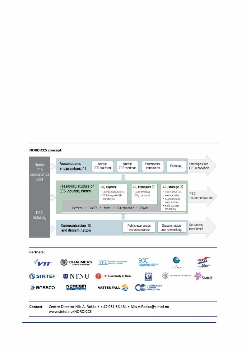
About NORDICCS

Nordic CCS Competence Centre, NORDICCS, is a networking platform for increased CCS deployment in the Nordic countries. NORDICCS has 10 research partners and six industry partners, is led by SINTEF Energy Research, and is supported by Nordic Innovation through the Top-level Research Initiative.

The views presented in this report solely represent those of the authors and do not necessarily reflect those of other members in the NORDICCS consortia, NORDEN, The Top Level Research Initiative or Nordic Innovation. For more information regarding NORDICCS and available reports, please visit http://www.sintef.no/NORDICCS.

Project 11029Project 11029

1 Introduction

In CO2 transport by pipeline, the massflow to be transported will vary with time, as well as thefluid properties. Each industrial site will produce varying quantities of CO2, containing impuritiesdepending on the site type and on the capture process. Besides, the different sites of a clustersending CO2 in a shared pipeline, will produce CO2 with different properties and in varyingquantities.

Impurities have an effect on the thermodynamical properties of the CO2 mixture, in particularon the phase envelope. This plays a role in whether the flow will remain in single phase. Thedesign should take into account the possible occurrence of two-phase flow, especially with corro-sive phases like water. Two-phase flow may also lead to unstable flow (slug, vertical flows,. . . ),and cause problems in compressors or pumps, etc.

Chaczykowski and Osiadacz [1] started to assess the effect of impurities in CO2 on the flowin pipelines. The present work systematises that study and investigates the effect of the fluidproperties on the flow during a slow transient. The test case run in the present work is inspiredfrom the varying load of a power plant. It is not in the scope of this work to study multiphaseflow. Therefore the flow is stopped when multiphase flow occurs.

Some of the present results were presented as a poster at the 7th Trondheim CCS Conference.

2 The models

The single-phase flow is modelled by the Euler equations

∂ρ

∂ t+

∂ (ρu)∂x

= 0, (1)

∂ (ρu)∂ t

+∂(ρu2 + p

)∂x

= τw, (2)

∂(ρ(e+ 1

2u2))∂ t

+∂(ρ(e+ 1

2u2)u+ pu)

∂x= Qw, (3)

where ρ is the fluid density, u is the velocity, p is the pressure and e is the internal energy. Thesource terms τw and Qw are the wall friction and the heat transfer from the wall to the fluid,respectively. The fluid thermodynamical state is described by the Soave-Redlich-Kwong (SRK)equation of state with van der Waals mixing rules (see for example [2, p.75, 85]). The physicalproperties, like the viscosity, the heat capacity and the heat conductivity are evaluated using theTRAPP model, which is a corresponding-states model [3, 4].

The Haaland approximation of the Colebrook correlation [5] gives the Darcy friction factor

fD =64Re

if Re < 2000, (4)

1√fD

=−1.8log10

[(ε/D3.7

)1.11

+6.9Re

]if Re≥ 2000, (5)

3

Project 11029Project 11029

and the friction term is given by the Darcy-Weisbach equation

τw = fD ·ρu2

2D. (6)

For the heat source term Qw, a transient wall temperature model is used, which is able to simulatethe heat transfer in the pipe material and in the soil. The heat transfer from the surroundingatmosphere is given by

Qatm = hatm(Tatm−Tw,o), (7)

where Tw,o is the pipe-wall or soil temperature in contact with the atmosphere, Tatm is the atmo-spheric temperature, and hatm is the heat transfer coefficient between the pipe-wall or the soil andthe atmosphere. The heat transfer between the fluid inside the pipe and the pipe wall is given by

Qw = h f (Tw,i−Tf ), (8)

where Tw,i is the pipe-wall temperature in contact with the fluid, Tf is the fluid temperature andh f is the heat-transfer coefficient between the fluid and the pipe wall. h f is given by the Nusseltnumber, which is found using the Dittus-Boelter correlation [6, 7]

Nu = 0.023Re0.8Pr0.4, (9)

where Nu is the Nusselt number, Re is the Reynolds number and Pr the Prandtl number. Thegeometry of the pipe and the soil are assumed to be annular.

At the inlet boundary condition, a pump is basically modelled by imposing the massflow andthe fluid temperature, while the pressure is extrapolated from the pipe. At the outlet, the boundarycondition is designed to mimic injection into a reservoir. Since the vertical flow is not modelled,the equivalent reservoir pressure is adjusted to the terrain altitude. The injected massflow is then,similarly to the model used in the Vedsted pipeline simulation [8], given by

m =(

ppipe− preservoir)

ki, (10)

where the reservoir pressure preservoir and the injectivity coefficient ki are fixed. Then, the mass-flow is imposed, while the thermodynamical state is extrapolated.

3 Case study

3.1 CO2 mixtures studied

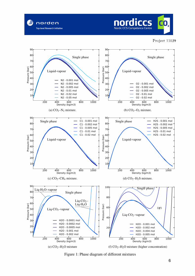
In the present work, we have looked at the flow of binary mixtures of CO2 with various impurities.The phase diagrams of several mixture are shown in Figure 1.

• CO2–N2 mixture in Figure 1a.

• CO2–O2 mixture in Figure 1b.

• CO2–CH4 mixture in Figure 1c.

4

Project 11029Project 11029

• CO2–H2S mixture in Figure 1d.

• CO2–H2O mixture in Figure 1e.

Note that in the single-phase region (above the equilibrium curve), the temperature increases fromright to left. On the CO2–H2O mixture phase diagram, also note the areas where a liquid water-rich phase exists. At higher water concentration (Figure 1f), the two areas with water-rich phasesmerge. The new area is denoted by (ϕ) in the Figure. Since the area (ϕ) stretches over the criticalpoint for CO2, the second phase is either vapour or liquid CO2.

3.2 Case definition

We study a flat 50 km-long pipeline, with 1.27 cm wall thickness and 20 cm inner diameter. Whenthe pipe is buried, the soil is a cylinder with a diameter of 1.27 m. The atmospheric temperatureis 20°C. The equivalent reservoir pressure at well head is 60 bar and the injectivity coefficient2.4×10−5 kg s/Pa. The physical properties of the pipe and the soil are summarised in Table 1.

Table 1: Physical properties of the pipe and soil

Pipe Soil

Density (kg/m3) 7850 1800Heat capacity (J/(kgK)) 470 1000Heat conductivity (W/(mK)) 45 2.6

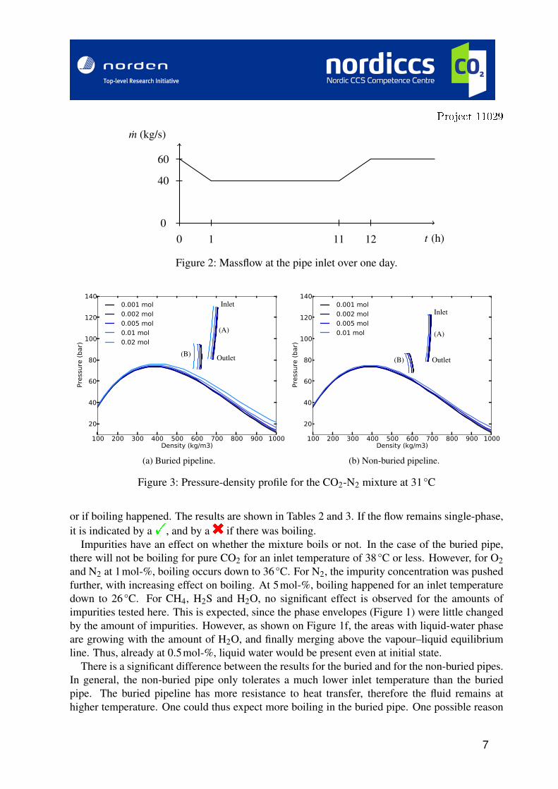
The pipe flow, as well as the wall and soil temperatures, are brought to steady state, with amassflow of 60 kg/s at a given inflow temperature. Then, the massflow is varied at the inletaccording to Figure 2. This is thought to reproduce the load variation of a power plant overone day. We then check if the flow remained in single phase over the whole cycle, or if boilingoccurred.

4 Results

4.1 Plots

As an example, the pipeline pressure-density profiles are plotted in the phase diagram, for dif-ferent concentrations of N2 in CO2 (Figure 3). The profile denoted by a (A) corresponds to theinitial steady state. The profile denoted by a (B) correspond to the state just before increasing themassflow again. The profile is plotted both in the case of the buried pipe and in the case of thenon-buried pipe. Boiling occurs when the outlet of the pipe goes under the equilibrium line.

4.2 Results for various compositions and temperatures

The test case has been run with different binary mixtures, amount of impurities, and inlet temper-atures. Then, it was determined if the flow had remained in single phase during the whole cycle,

5

Project 11029Project 11029

200 400 600 800 1000Density (kg/m3)

10

20

30

40

50

60

70

80

90

Pre

ssure

(bar)

N2 - 0.001 mol

N2 - 0.002 mol

N2 - 0.005 mol

N2 - 0.01 mol

N2 - 0.02 mol

N2 - 0.05 mol

Liquid-vapour

Single phase

(a) CO2–N2 mixture.

200 400 600 800 1000Density (kg/m3)

10

20

30

40

50

60

70

80

90

Pre

ssure

(bar)

O2 - 0.001 mol

O2 - 0.002 mol

O2 - 0.005 mol

O2 - 0.01 mol

O2 - 0.02 mol

Liquid-vapour

Single phase

(b) CO2–O2 mixture.

200 400 600 800 1000Density (kg/m3)

10

20

30

40

50

60

70

80

90

Pre

ssure

(bar)

C1 - 0.001 mol

C1 - 0.002 mol

C1 - 0.005 mol

C1 - 0.01 mol

C1 - 0.02 mol

Liquid-vapour

Single phase

(c) CO2–CH4 mixture.

200 400 600 800 1000Density (kg/m3)

10

20

30

40

50

60

70

80

90

Pre

ssure

(bar)

H2S - 0.001 mol

H2S - 0.002 mol

H2S - 0.005 mol

H2S - 0.01 mol

H2S - 0.02 mol

Liquid-vapour

Single phase

(d) CO2–H2S mixture.

200 400 600 800 1000Density (kg/m3)

10

20

30

40

50

60

70

80

90

Pre

ssure

(bar)

H2O - 0.0001 mol

H2O - 0.0002 mol

H2O - 0.0005 mol

H2O - 0.001 mol

H2O - 0.002 mol

Liq-CO2–vapour

Single phaseLiq-H2O–vapour

Liq-CO2–Liq-H2O

(e) CO2–H2O mixture

200 400 600 800 1000Density (kg/m3)

20

40

60

80

100

Pre

ssure

(bar)

H2O - 0.001 mol

H2O - 0.002 mol

H2O - 0.004 mol

H2O - 0.005 mol

Liq-CO2–vapour

Single phase

(ϕ)

(f) CO2–H2O mixture (higher concentration)

Figure 1: Phase diagram of different mixtures

6

Project 11029Project 11029

m (kg/s)

t (h)

60

40

00 1 11 12

Figure 2: Massflow at the pipe inlet over one day.

100 200 300 400 500 600 700 800 900 1000Density (kg/m3)

20

40

60

80

100

120

140

Pre

ssure

(bar)

0.001 mol

0.002 mol

0.005 mol

0.01 mol

0.02 mol

(A)

(B)

Inlet

Outlet

(a) Buried pipeline.

100 200 300 400 500 600 700 800 900 1000Density (kg/m3)

20

40

60

80

100

120

140Pre

ssure

(bar)

0.001 mol

0.002 mol

0.005 mol

0.01 mol (A)

(B)

Inlet

Outlet

(b) Non-buried pipeline.

Figure 3: Pressure-density profile for the CO2-N2 mixture at 31°C

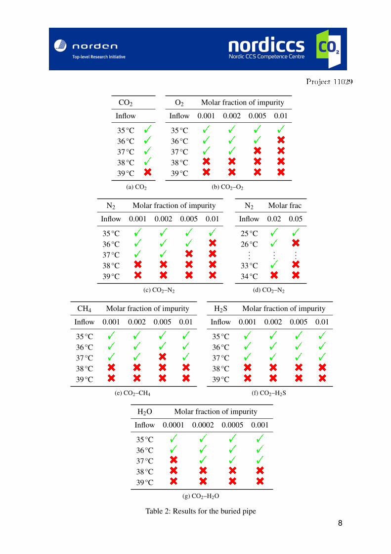
or if boiling happened. The results are shown in Tables 2 and 3. If the flow remains single-phase,it is indicated by a!, and by a$ if there was boiling.

Impurities have an effect on whether the mixture boils or not. In the case of the buried pipe,there will not be boiling for pure CO2 for an inlet temperature of 38°C or less. However, for O2and N2 at 1mol-%, boiling occurs down to 36°C. For N2, the impurity concentration was pushedfurther, with increasing effect on boiling. At 5mol-%, boiling happened for an inlet temperaturedown to 26°C. For CH4, H2S and H2O, no significant effect is observed for the amounts ofimpurities tested here. This is expected, since the phase envelopes (Figure 1) were little changedby the amount of impurities. However, as shown on Figure 1f, the areas with liquid-water phaseare growing with the amount of H2O, and finally merging above the vapour–liquid equilibriumline. Thus, already at 0.5mol-%, liquid water would be present even at initial state.

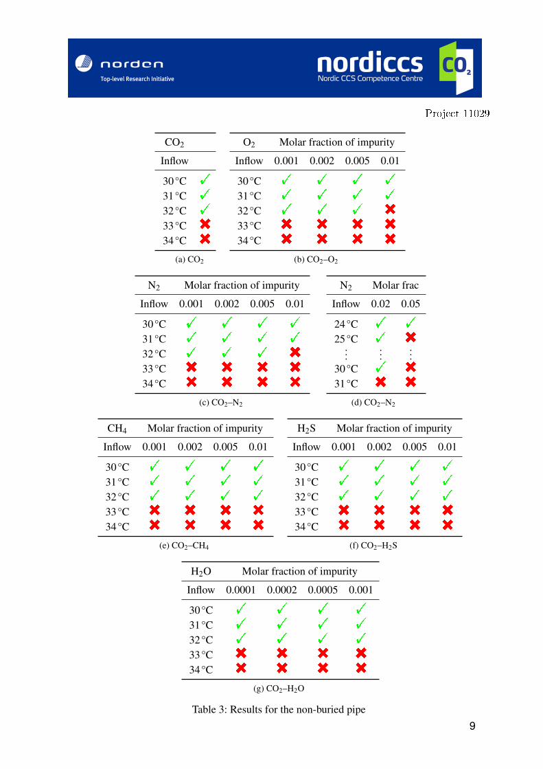
There is a significant difference between the results for the buried and for the non-buried pipes.In general, the non-buried pipe only tolerates a much lower inlet temperature than the buriedpipe. The buried pipeline has more resistance to heat transfer, therefore the fluid remains athigher temperature. One could thus expect more boiling in the buried pipe. One possible reason

7

Project 11029Project 11029

CO2

Inflow

35°C !

36°C !

37°C !

38°C !

39°C $

(a) CO2

O2 Molar fraction of impurity

Inflow 0.001 0.002 0.005 0.01

35°C ! ! ! !

36°C ! ! ! $

37°C ! ! $ $

38°C $ $ $ $

39°C $ $ $ $

(b) CO2–O2

N2 Molar fraction of impurity

Inflow 0.001 0.002 0.005 0.01

35°C ! ! ! !

36°C ! ! ! $

37°C ! ! $ $

38°C $ $ $ $

39°C $ $ $ $

(c) CO2–N2

N2 Molar frac

Inflow 0.02 0.05

25°C ! !

26°C ! $...

......

33°C ! $

34°C $ $

(d) CO2–N2

CH4 Molar fraction of impurity

Inflow 0.001 0.002 0.005 0.01

35°C ! ! ! !

36°C ! ! ! !

37°C ! ! $ !

38°C $ $ $ $

39°C $ $ $ $

(e) CO2–CH4

H2S Molar fraction of impurity

Inflow 0.001 0.002 0.005 0.01

35°C ! ! ! !

36°C ! ! ! !

37°C ! ! ! !

38°C $ $ $ $

39°C $ $ $ $

(f) CO2–H2S

H2O Molar fraction of impurity

Inflow 0.0001 0.0002 0.0005 0.001

35°C ! ! ! !

36°C ! ! ! !

37°C $ ! ! !

38°C $ $ $ $

39°C $ $ $ $

(g) CO2–H2O

Table 2: Results for the buried pipe

8

Project 11029Project 11029

CO2

Inflow

30°C !

31°C !

32°C !

33°C $

34°C $

(a) CO2

O2 Molar fraction of impurity

Inflow 0.001 0.002 0.005 0.01

30°C ! ! ! !

31°C ! ! ! !

32°C ! ! ! $

33°C $ $ $ $

34°C $ $ $ $

(b) CO2–O2

N2 Molar fraction of impurity

Inflow 0.001 0.002 0.005 0.01

30°C ! ! ! !

31°C ! ! ! !

32°C ! ! ! $

33°C $ $ $ $

34°C $ $ $ $

(c) CO2–N2

N2 Molar frac

Inflow 0.02 0.05

24°C ! !

25°C ! $...

......

30°C ! $

31°C $ $

(d) CO2–N2

CH4 Molar fraction of impurity

Inflow 0.001 0.002 0.005 0.01

30°C ! ! ! !

31°C ! ! ! !

32°C ! ! ! !

33°C $ $ $ $

34°C $ $ $ $

(e) CO2–CH4

H2S Molar fraction of impurity

Inflow 0.001 0.002 0.005 0.01

30°C ! ! ! !

31°C ! ! ! !

32°C ! ! ! !

33°C $ $ $ $

34°C $ $ $ $

(f) CO2–H2S

H2O Molar fraction of impurity

Inflow 0.0001 0.0002 0.0005 0.001

30°C ! ! ! !

31°C ! ! ! !

32°C ! ! ! !

33°C $ $ $ $

34°C $ $ $ $

(g) CO2–H2O

Table 3: Results for the non-buried pipe

9

Project 11029Project 11029

for that is that a higher temperature maintains a lower density, hence a higher fluid velocity andhigher friction. This increases pressure drop and thus pressure in the pipe, which leads to lessboiling. All in all, the pipe environment is very important in this test case. Note though thatthe effect of soil almost disappears for N2 at 5mol-%, where boiling happens close to the inlettemperature.

5 Conclusions

A single-phase flow simulation tool was used to assess the occurrence of boiling in a CO2 pipelineduring slow load variations. Different binary mixtures of CO2 plus an impurity have been studied,with different concentrations of the impurity.

The occurrence of multiphase flow in CO2 mixtures depends on the kind and amount of impu-rities present. The first and main reason is that the phase envelope is modified by the impurities– generally, boiling happens at higher pressure. The second reason is that the thermophysicalproperties change with impurities. For example, heat conductivity, viscosity or density. Heatexchange with the environment also plays a significant role.

Robust fluid- and thermodynamical simulation tools are needed to to predict the flow behaviourof the CO2 during transients. In the present work, we have limited ourselves to the questionwhether two-phase flow will occur or not. The next step is to assess the effect of impurities in atwo-phase flow, for example on cooling of the pipe.

References

[1] M. Chaczykowski and A. J. Osiadacz, “Dynamic simulation of pipelines containing densephase/supercritical CO2-rich mixtures for carbon capture and storage,” International Journalof Greenhouse Gas Control, vol. 9, pp. 446–456, July 2012.

[2] M. L. Michelsen and J. M. Mollerup, Thermodynamic models: Fundamentals & computa-tional aspects. Tie-Line Publications, 2007.

[3] J. F. Ely and H. J. M. Hanley, “Prediction of transport properties. 1. viscosity of fluids andmixtures,” Industrial & Engineering Chemistry Fundamentals, vol. 20, pp. 323–332, Nov.1981.

[4] J. F. Ely and H. J. M. Hanley, “Prediction of transport properties. 2. thermal conductivityof pure fluids and mixtures,” Industrial & Engineering Chemistry Fundamentals, vol. 22,pp. 90–97, Feb. 1983.

[5] S. E. Haaland, “Simple and explicit formulas for the friction factor in turbulent pipe flow,”Journal of Fluids Engineering – Transactions of the ASME, vol. 105, pp. 89–90, 1983.

[6] F. W. Dittus and L. M. K. Boelter, “Heat transfer in automobile radiators of the tubular type,”University of California Publications in Engineering, vol. 2, pp. 443–461, 1930.

[7] W. H. McAdams, Heat Transmission. New York: McGraw-Hill, second ed., 1942.

10

Project 11029Project 11029

[8] L. Klinkby, C. M. Nielsen, E. Krogh, I. E. Smith, B. Palm, and C. Bernstone, “Simulat-ing rapidly fluctuating CO2 flow into the vedsted CO2 pipeline, injection well and reser-voir,” in GHGT-10 – 10th International Conference on Greenhouse Gas Control Technologies(J. Gale, C. Hendriks, and W. Turkenberg, eds.), (Amsterdam, The Netherlands), pp. 4291–4298, IEAGHGT, Energy Procedia vol. 4, 2011.

11