Embed Size (px)
Citation preview
Depressurisation of CO2-pipelines with volatile gas impurities: Temperature
behavior
Eskil Aursand
NORDICCS Technical Report D5.2.1302
December 2013
Summary This memo is a computational study of the depressurisation of high-pressure pipelines containing CO2 with volatile gas impurities such as N2, CH4 and O2. The focus is on how variables such as kind and amount of impurity affect the temperatures occurring inside the pipeline during depressurisation, and how this compares to the effect of varying the valve size, i.e. the rate of outflow. The flow was simulated by solving an equilibrium two-fluid two-component 1D flow model, with additional source terms accounting for valve outflow, friction, and wall heat transfer. The results showed that adding volatile gas impurities to pure CO2 slighly reduces the amount of depressurisation temperature-drop, while slightly increasing the speed at which this drop occurs. However, these effects were negligible compared to the effect of slight changes in valve opening radius. It remains to be seen how other much less volatile impurities such as NOx, SOx, H2S and H2O will affect the temperature drop.
Keywords Fluid dynamics, thermodynamics, impurities, CO2 transport, depressurisation.
Authors Eskil Aursand, SINTEF Energy Research, Norway, [email protected] Date December 2013
About NORDICCS
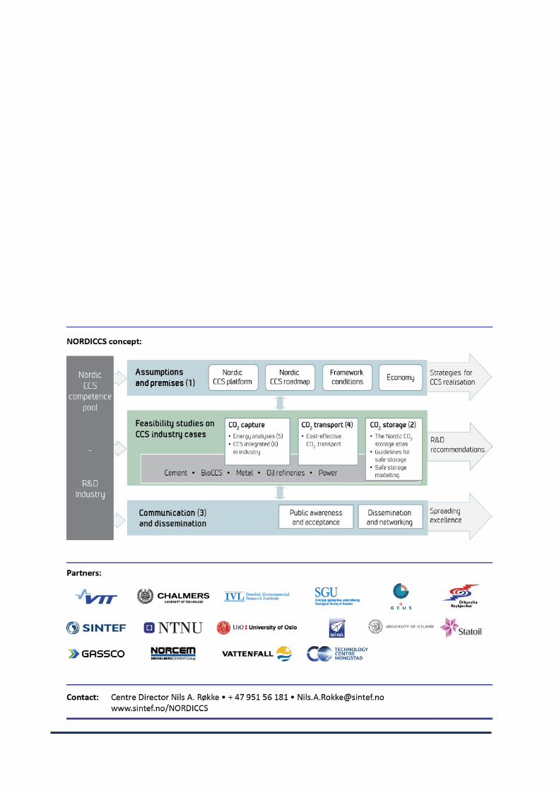
Nordic CCS Competence Centre, NORDICCS, is a networking platform for increased CCS deployment in the Nordic countries. NORDICCS has 10 research partners and six industry partners, is led by SINTEF Energy Research, and is supported by Nordic Innovation through the Top-level Research Initiative.
The views presented in this report solely represent those of the authors and do not necessarily reflect those of other members in the NORDICCS consortia, NORDEN, The Top Level Research Initiative or Nordic Innovation. For more information regarding NORDICCS and available reports, please visit http://www.sintef.no/NORDICCS.
Project 11029Project 11029
Contents
1 Introduction 4
2 The model 52.1 Flow equations . . . . . . . . . . . . . . . . . . . . . . . . . . . . . . . . . . . 5
2.1.1 Thermodynamics and thermophysical properties . . . . . . . . . . . . . 62.1.2 Numerics . . . . . . . . . . . . . . . . . . . . . . . . . . . . . . . . . . 7
2.2 Source terms . . . . . . . . . . . . . . . . . . . . . . . . . . . . . . . . . . . . 72.2.1 Depressurisation valve . . . . . . . . . . . . . . . . . . . . . . . . . . . 72.2.2 Wall heat transfer . . . . . . . . . . . . . . . . . . . . . . . . . . . . . . 92.2.3 Friction momentum exchange . . . . . . . . . . . . . . . . . . . . . . . 9
3 Simulation cases 9
4 Grid sensitivity test 10
5 Results 125.1 General behaviour . . . . . . . . . . . . . . . . . . . . . . . . . . . . . . . . . . 125.2 Effect of impurities . . . . . . . . . . . . . . . . . . . . . . . . . . . . . . . . . 135.3 Effect of valve opening . . . . . . . . . . . . . . . . . . . . . . . . . . . . . . . 13
6 Discussion 18
7 Conclusions 187.1 Suggestions for further work . . . . . . . . . . . . . . . . . . . . . . . . . . . . 19
References 19
3
Project 11029Project 11029
1 Introduction
CO2 may be transported by pipeline in its liquid or supercritical form. This implies high operatingpressures, in the order of 100atm. In such a transport system, depressurisations may occur, ei-ther intentionally for shutdown or maintenance, or by accident due to leakage through a damagedsection of the pipeline. In the event of such rapid depressurisations/expansions, a fluid will expe-rience a decrease in temperature through the Joule-Thomson effect. Additionally, as gas escapesthe pipeline, the liquid boils to fill the vacant volume, absorbing the needed latent heat in theprocess. When these temperature-reducing effects are able to overcome the rate of heat transferfrom the surroundings, we have what is called auto-refrigeration. Eventually, when all of the gashas vaporised, and most of it has escaped the pipeline, the heat transfer from the surroundingswill make the temperature start to increase again.
The above implies that there is a certain minimum temperature occurring in the pipeline atsome location and time. It is of interest to predict this lowest temperature for various safetyreasons, including ensuring operation above the ductile–brittle transition temperature (DBTT) ofthe pipeline steel [1], preventing brittle fractures in welds, preventing the formation of ice andhydrates, and generally staying inside the temperature design-specifications of all the equipmentinvolved. Additionally, a high rate of temperature decrease may also be demanding on materialsand equipment.
CO2 transported by pipeline is rarely 100% pure, especially not when coming from capture-processes in a Carbon Capture and Storage (CCS) system. The presence of impurities will influ-ence the thermodynamic behaviour of the fluid compared to pure CO2 [2], and is thus expectedto influence the auto-refrigeration when depressurising a pipeline. This work does not cover theeffect of all possible impurities, but is limited in scope to N2, CH4 and O2, which represent whatwill be called the volatile gas impurities. By this we mean that their own boiling-points are lo-cated at much lower temperatures than the ones reached in these depressurisation events. In theirpure form, they would not undergo any phase transition (boiling), but rather be in a gas or super-critical gas-like state throughout the event. This is in contrast to CO2, which exists as a denseliquid or supercritical liquid-like phase at ordinary operating conditions, and will inevitably beginto boil during such depressurisations.
The effect of impurities should not be studied in isolation, but also compared to the effect ofvarying other relevant parameters. In this work, the effect of impurity kind and amount on thetemperature-behaviour will be compared to the effect of varying the outflow area, e.g. the valveopening. In deliberate depressurisation, this is a directly controllable parameter which could beused to offset any negative impurity effects.
The present memo is a computational study, employing multi-phase computational fluid dy-namics and thermodynamics. The work relates to the previous NORDICCS deliverable D5.2.1301by Morin [3], who investigated the possibility of initiating multi-phase flow due to variable flowrates during regular transport to an injection site. In that study, the onset of multi-phase flow wasmerely noted, and not actually simulated any further. In the depressurisation events studied here,multi-phase flow is inevitable, and its dynamics must be simulated.
4
Project 11029Project 11029
2 The model
The depressurisation events are modelled by one-dimensional computational fluid dynamics, ac-counting for phase transfer and thermodynamic effects, flow of liquid and vapour at differentvelocities, momentum transfer by friction, heat transfer through pipeline walls, and the loss ofmass, momentum and energy though a depressurisation valve.
2.1 Flow equations
The set of governing equations used for the pipeline flow is a two-fluid two-component flowmodel [4], with additional source terms for valve outflow, friction, and wall heat transfer, with theassumption of instantaneous local mechanical, thermal and chemical equilibrium:
∂ (ρgαgz1,g)
∂ t+
∂ (ρgαgz1,g)ug
∂x=−ζρ,1,g, (1a)
∂ (ρgαgz2,g)
∂ t+
∂ (ρgαgz2,g)ug
∂x=−ζρ,2,g, (1b)
∂ (ρlαgz1,l)
∂ t+
∂ (ρlαlz1,l)ul
∂x=−ζρ,1,l, (1c)
∂ (ρlαgz2,l)
∂ t+
∂ (ρlαlz2,l)ul
∂x=−ζρ,2,l, (1d)
∂ (ρgαgug)
∂ t+
ρgαgu2g
∂x+αg
∂ p∂x
+ τi =−τg,w− τg,l−ζρu,g, (1e)
∂ (ρlαlul)
∂ t+
ρlαlu2l
∂x+αl
∂ p∂x− τi =−τl,w + τg,l−ζρu,l, (1f)
∂ (Eg +El)
∂ t+
∂ (Egug +αgug p)∂x
+∂ (Elul +αlul p)
∂x= ζE +Qw. (1g)
Subscripts g and l refer to gas phase and liquid phase, respectively, while subscripts 1 and 2indicate chemical components. With k as a generalised phase subscript, ρk (kg/m3) is the densityof phase k, while αk and wk are the volume and mass fractions of phase k, i.e.
αk ≡Vk
Vm, wk ≡
mk
mm, (2)
satisfying∑k
αk = 1, ∑k
wk = 1, (3)
and are related bywk
αk=
ρk
ρm(4)
for any phase k. A subscript m indicates a total for the local mixture. An example is ρm, which isthe mixture density given by
ρm = ∑k
αkρk. (5)
5
Project 11029Project 11029
Mass fractions of components within phases are given by
zi,k ≡mi,k
mk(6)
satisfying∑
izi,k = 1. (7)
The variable uk (m/s) is the velocity of phase k, p (Pa) is the pressure, and Ek (J/m3) is thetotal energy per volume of phase k, i.e.
Ek = αkρk(ek +u2
k/2), (8)
where ek (J/kg) is the internal energy per mass of phase k. Finally, for the left hand side of (1),we have τi (kg(m/s)/(m3s)) , which is the interfacial momentum exchange. This may be modelledas [4]
τi =−∆pi∂αl
∂x, (9)
where ∆pi is the difference between the average pressure and the pressure at the gas-liquid inter-face, here estimated by the average liquid hydrostatic pressure:
∆pi =12
Dαlρlg. (10)
Here g is the gravitational acceleration and D is the pipeline diameter.The right hand side of (1) contains source terms representing valve leakage (ζ ), friction (τ) and
wall heat transfer (Qw). These are described more closely in Sec. 2.2.The flow model (1) is solved numerically as detailed in Sec. 2.1.2. After the flow model
has evolved for one time step, the two phases will generally be out of chemical equilibrium.Therefore, the phase change needed to restore chemical equilibrium is calculated and appliedbetween each time step, using an equation of state (Sec. 2.1.1). This is called the fractional-stepor time-splitting method.
The boundary conditions of the one-dimensional flow model represent stationary walls orclosed valves. The opening causing the depressurisation event is a valve at the x = 0 end ofthe pipeline, though positioned on the side-wall, perpendicular to the pipeline axis. The initialcondition is a spatially constant temperature-pressure state in the pure liquid/dense phase area,with zero velocity.
2.1.1 Thermodynamics and thermophysical properties
The common Soave-Redlich-Kwong (SRK) [5] cubic Equation of State (EoS) with Van der Waalsmixing rules [6] is used to describe the mixture behaviour.
The instantaneous thermodynamic equilibrium is maintained by performing an energy-densityflash calculation after each time-step of the numerical solving of (1). This entails using themixture density and total energy known from the flow equations to calculate new state propertiessuch as pressure, temperature, volume fractions, phase compositions and new phase velocities.
The thermophysical properties such as viscosity and heat conductivity are calculated by theTRAPP corresponding-states model [7, 8].
6
Project 11029Project 11029
2.1.2 Numerics
Time-integration of the flow equations (1) is done with the simple Forward Euler method, withthe time-step obeying a Courant–Friedrichs–Lewy (CFL) condition
∆t =C∆x
max(|cmix±uk|), (11)
where ∆x is the length of a computational cell and cmix is an approximate local speed of soundfor the phase mixture, as given by (3.74) in [4]. The function max() implies finding the maximumvalue across the pipeline for either phase, at the given time. The condition is set with a constantCFL-number C = 0.5.
The spatial numerical scheme is according to the FORCE-flux method [9], extended to handlenon–conservative terms [10].
2.2 Source terms
The source terms are all the terms on the right hand side of the flow equations (1). The termsrepresenting valve leakage (ζ ) are covered in 2.2.1, the term representing wall heat transfer (Qw)is covered in 2.2.2, and the terms representing friction (τ) are covered in 2.2.3.
2.2.1 Depressurisation valve
The outflow through the valve is assumed to be isentropic, and we must then take into accountthe phenomenon of choked flow, where the fluid velocity at the valve is unable to increase beyondthe local speed of sound, no matter the pressure difference 1.
We employ an isentropic homogeneous equilibrium choke model, in which a fluid elementflows from inside the pipe at an initial pressure pi = p(x) to the point of escape at the unknownescape-pressure pe(x). The escape pressure is within the range [pa, pi] if the flow is choked,and equal to pa if not, with pa denoting the atmospheric pressure. The initial velocity for thestreamline is taken as a weighted average of the gas and liquid velocities at that point in the flowequations:
u0 =∑k αkρkuk
∑k αkρk(12)
Assuming instantaneous equilibrium and equal liquid/vapor velocity in the outflow process, andusing the fact that the escape velocity is equal to the local speed of sound when the outflow ischoked, we may find the the choke pressure as
pe =
{p ∈ [pi, pa] :
ddp
[ρm(p,s0)
2(∫ p
pi
dp′
ρm(p′,so)− 1
2u2
0
)]= 0}, (13)
i.e. the choke pressure is the pressure at which the expression in the above square parenthesisreaches its minimum value (the integral is negative). The function ρm(p,s) is provided by theequation of state. Here so is the specific entropy inside the pipeline, i.e. corresponding to the
1However, increased upstream pressure may increase the local speed of sound, thus allowing faster escape velocity.
7
Project 11029Project 11029
current 1D flow variables. If no such maximum can be found, the flow is not choked, and pe = pa.In the process of finding pe, ρe is also found as the mixture density at the escape point. Once theescape pressure pe has been found, the escape fluid velocity may be found from Bernoulli’sprinciple as
ue =
√u2
0−2∫ pe
pi
dp′
ρm(p′,so). (14)
The escape velocity found from (14) is interpreted as the absolute speed at the escape point, whichmay have an x-component and a y-component.
These escape quantities, pe, ρe and ue, must now somehow be interpreted as source termsin (1). If one considers the integral form of the conservation equations for a homogeneous fluid,one finds with some simplifying assumptions, while ensuring that the specific entropy within thepipeline is conserved, that the source terms are:
ζρ =
(−ρeuy,eAe
Vcell
),
ζρu =
(−ρeuy,eAe
Vcell
)·u0,
ζE =
(−ρeuy,eAe
Vcell
)·(
e+pρ+
12
u2x
), (15)
where Ae is the valve opening area, Vcell is the volume of the computational cell containing thevalve, and the y-component of the escape velocity is given by
uy,e =√
u2e−u2
0. (16)
In order to use this in (1), the source terms for mass and momentum have to be distributedbetween the multiple mass and momentum equations. The mass source term is distributed amongthe first source terms in (1) according to
ζρ,i,k
ζρ
=mi,k
mm= wk · zi,k, (17)
i.e. weighted by the ratio of mass of component i in phase k to the total mass, as given by thestate in the pipeline cell. Similarly, the momentum source term is distributed according to
ζρu,k
ζρu=
αkρkuk
∑k αkρkuk, (18)
i.e. weighted by the ratio of momentum in the given phase to the total momentum.The energy source term ζE does not need to be distributed, as there is only one equation for
energy conservation.
8
Project 11029Project 11029
2.2.2 Wall heat transfer
The heat transfer model is completely axisymmetric, with a shell representing the pipeline wallinside a shell representing the soil around the buried pipeline. The soil shell is an approximationto the real situation, which is a flat soil surface some distance above and essentially infinite lengthsof soil in other directions.
The heat transfer between the fluid and the pipeline wall is calculated through
q = hi(Tw−T ) (19)
where q(W/m2) is the amount of heat transfer rate into the fluid per area of pipeline wall, andTw(K) is the pipeline inner wall temperature. The inner heat transfer coefficient, hi(W/(m2K)),is calculated based on the Colburn correlation [11], using volume-averaged properties as input.
The source term Qw(W/m3) in (1g) is the heat transfer rate per volume of fluid, i.e.
Qw =Aw
Vcellq =
2πridxπr2
i dxq =
2ri
q =2ri
hi(Tw−T ) (20)
where Ae is the wall heat transfer area, and ri is the inner radius of the pipeline.The temperature profile at the inside of the solids (pipeline metal and soil) is calculated tran-
siently by integrating the axially symmetric heat conduction equation from the temperature profilein the previous time step. The heat transfer between air and soil is calculated from a constant out-side heat transfer coefficient.
Note that only radial heat conduction is included, i.e. there is no conduction along the pipelineaxis, between computational cells. However, convective axial heat transfer is included in (1).
2.2.3 Friction momentum exchange
This section briefly explains the calculation of the friction terms in the flow equations (1), whichinclude τg,w (gas-to-wall momentum transfer), τl,w (liquid-to-wall momentum transfer), and τg,l(gas-to-liquid momentum transfer).
Where the flow is single-phase, τg,l = 0, and τk,w is calculated from the Darcy-Weisbach equa-tion. The Haaland friction factor [12] with a relative roughness factor of 5×10⁻⁵ is used wherethe flow is turbulent, and a friction factor of 64/Re is used where the flow is laminar.
Where there is two-phase flow, the three friction terms are calculated from the Spedding &Hand two-fluid friction model [13].
3 Simulation cases
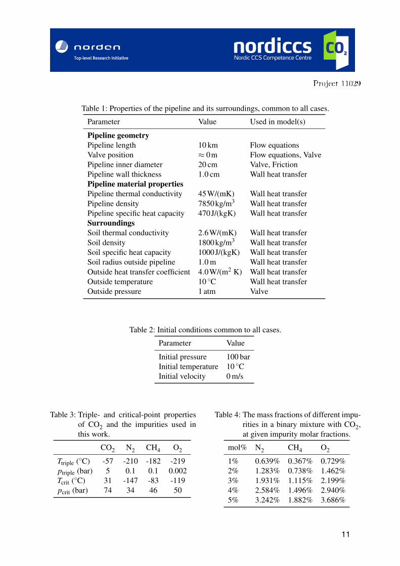
The cases simulated in this work is the depressurisation/emptying of a 10 km pipeline containinga binary mixture of CO2 with an impurity. The pipeline section has been closed off at the ends inthe axial direction, and the emptying is performed by opening a perpendicular valve close to oneend. The full set of case parameters common to all simulations are shown in Tab. 1. The initialstate of the fluid is as listed in Tab. 2.
9
Project 11029Project 11029
The impurities studied here are N2, CH4 and O2. These are all considerably more volatile gasesthan CO2. The temperature ranges encountered in the simulations in this work are all well abovethe critical temperatures of the impurities alone, while below the critical temperature of CO2 (seeTab. 3). Note that when impurity concentrations are shown without further explanation, they areimplicitly molar fractions. The corresponding mass fractions will depend on the molar masses ofthe substances involved (see Tab. 4).
4 Grid sensitivity test
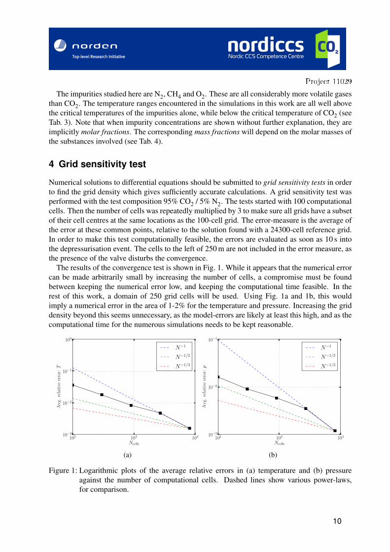
Numerical solutions to differential equations should be submitted to grid sensitivity tests in orderto find the grid density which gives sufficiently accurate calculations. A grid sensitivity test wasperformed with the test composition 95% CO2 / 5% N2. The tests started with 100 computationalcells. Then the number of cells was repeatedly multiplied by 3 to make sure all grids have a subsetof their cell centres at the same locations as the 100-cell grid. The error-measure is the average ofthe error at these common points, relative to the solution found with a 24300-cell reference grid.In order to make this test computationally feasible, the errors are evaluated as soon as 10 s intothe depressurisation event. The cells to the left of 250 m are not included in the error measure, asthe presence of the valve disturbs the convergence.
The results of the convergence test is shown in Fig. 1. While it appears that the numerical errorcan be made arbitrarily small by increasing the number of cells, a compromise must be foundbetween keeping the numerical error low, and keeping the computational time feasible. In therest of this work, a domain of 250 grid cells will be used. Using Fig. 1a and 1b, this wouldimply a numerical error in the area of 1-2% for the temperature and pressure. Increasing the griddensity beyond this seems unnecessary, as the model-errors are likely at least this high, and as thecomputational time for the numerous simulations needs to be kept reasonable.
102 103 104
Ncells
10−3
10−2
10−1
100
Avg
.re
lati
veer
ror:T
N−1
N−1/2
N−1/3
(a)
102 103 104
Ncells
10−3
10−2
10−1
Avg
.re
lati
veer
ror:p
N−1
N−1/2
N−1/3
(b)
Figure 1: Logarithmic plots of the average relative errors in (a) temperature and (b) pressureagainst the number of computational cells. Dashed lines show various power-laws,for comparison.
10
Project 11029Project 11029
Table 1: Properties of the pipeline and its surroundings, common to all cases.
Parameter Value Used in model(s)
Pipeline geometryPipeline length 10 km Flow equationsValve position ≈ 0m Flow equations, ValvePipeline inner diameter 20 cm Valve, FrictionPipeline wall thickness 1.0 cm Wall heat transferPipeline material propertiesPipeline thermal conductivity 45W/(mK) Wall heat transferPipeline density 7850kg/m3 Wall heat transferPipeline specific heat capacity 470J/(kgK) Wall heat transferSurroundingsSoil thermal conductivity 2.6W/(mK) Wall heat transferSoil density 1800kg/m3 Wall heat transferSoil specific heat capacity 1000J/(kgK) Wall heat transferSoil radius outside pipeline 1.0 m Wall heat transferOutside heat transfer coefficient 4.0W/(m2 K) Wall heat transferOutside temperature 10 ◦C Wall heat transferOutside pressure 1 atm Valve
Table 2: Initial conditions common to all cases.
Parameter Value
Initial pressure 100 barInitial temperature 10 ◦CInitial velocity 0 m/s
Table 3: Triple- and critical-point propertiesof CO2 and the impurities used inthis work.
CO2 N2 CH4 O2
Ttriple (◦C) -57 -210 -182 -219ptriple (bar) 5 0.1 0.1 0.002Tcrit (◦C) 31 -147 -83 -119pcrit (bar) 74 34 46 50
Table 4: The mass fractions of different impu-rities in a binary mixture with CO2,at given impurity molar fractions.
mol% N2 CH4 O2
1% 0.639% 0.367% 0.729%2% 1.283% 0.738% 1.462%3% 1.931% 1.115% 2.199%4% 2.584% 1.496% 2.940%5% 3.242% 1.882% 3.686%
11
Project 11029Project 11029
5 Results
The model described in Sec. 2 was run on a set of cases as described in Sec. 3. First, the generalqualitative behaviour of these cases is described Sec 5.1. Then, two kinds of parameter variationsare performed:
• Varying the kind and amount of impurity, while keeping the valve area at a constant 50cm2
(Sec. 5.2).
• Varying the valve area, while keeping the composition at 2 mol% N2 (Sec. 5.3).
The focus was on how these parameters influenced the temperatures reached in the pipeline duringthe depressurisation.
5.1 General behaviour
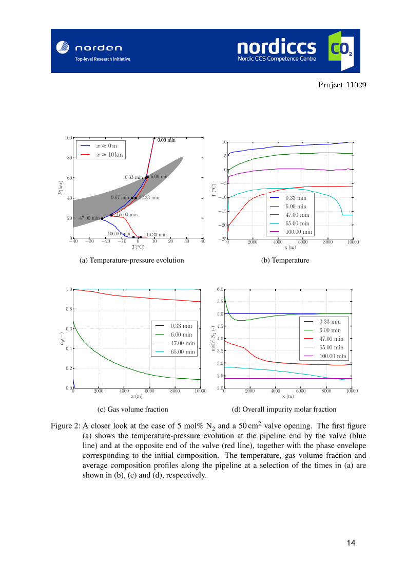
The qualitative behaviour of these simulations with different kinds and amounts of volatile gasimpurities is quite similar. In this section, this behaviour will be outlined using the case of 5mol% N2 and a 50 cm2 valve opening.
Figure 2a shows the temperature-pressure (TP) evolution in this case, close to the valve at oneend, and at the opposite end. These lines are shown together with a map of the two-phase region,i.e. the phase envelope. For each line, the marked points show, in chronological order, the initialstate, the onset of boiling, the point of reaching 40 bar, the end of boiling, and the point of reachingwithin 1% of 1 atm. The temperature, gas volume fraction and average composition profiles alongthe pipeline at a selection of these times are shown in Fig. 2b, 2c and 2d, respectively.
Some important phases/events in this case should be mentioned:
• The opening of the valve at x = 0 causes a sudden local pressure drop, and initiates apressure wave. This pressure wave carries the first information about the valve-openingevent through the pipeline, and its front moves at the initial speed of sound in the mixture,about 450m/s. After about 20 s, the wave reaches the other end, and the entire 10 kmpipeline “knows” about the event.
• After about 20 s the TP-state in the pipeline at x ≈ 0 reaches the bubble line, and starts toboil. Note that the actual outflow stream through the valve has involved boiling since thebeginning, but this event signifies the onset of boiling inside the pipeline.
• After approximately 47 min the first case of a local pure gas state occurs, at x ≈ 0. Theregion of pure gas proceeds to spread smoothly towards the other end of the pipeline, untilall liquid is gone at approximately 65 min.
• After approximately 2 h, the entire 10 km pipeline reaches atmospheric pressure. At thispoint, the gas is still at the reduced temperature of approximately 0 ◦C, and continues toapproach the ambient 10 ◦C for some hours.
Note that the phase envelope in Fig. 2a corresponds to the initial 5% composition, while theactual average composition2 varies in time and space as the simulations proceeds. The variations
2Average composition means composition in a pipeline section as a whole, i.e. the sum of moles of the givencomponent over all present phases, relative to the total number of moles of any kind present in the same volume.
12
Project 11029Project 11029
in average composition is due to the fact that in regions of two-phase states, the gas phase and theliquid phase will have different compositions from the local average composition. In this case,the gas phase will be richer in the volatile impurity, while the liquid phase will be richer in CO2.Since the model in (1) allows for different velocities of the phases, components can be transportedin rates out of proportion with its fraction of the average composition, leading to inhomogeneousaverage composition.
However, as seen in Fig. 2a, the TP-paths still align quite well with the initial phase envelope.The match of the bubble line is due to the fact that the flow has been single-phase liquid so far, andin single phase the average composition is equal to the phase composition, making a componentseparation impossible. At the time of dew line encounter, the average compositions have changedconsiderably, but the correspondence is still good because the low-temperature parts of the dewline are quite composition-independent in these mixtures (as seen later in Fig 3 b,d,f).
In this case, the ouflow has an impurity concentration higher than the initial 5%. This is becausethe outflow occurs where the valve is (x = 0), which is a region of high gas fraction due to thepressure drop. Since the gas is impurity rich, more impurity is lost through the valve compared tothe case of simply removing mixture of the initial average composition. This is seen in Fig. 2d,where the average mol% N2 drops from 5% to less than 2.5% before the depressurisation iscomplete. Note also how the mol% N2 is initially increased from the initial value at the valve,due to the rapid transport of N2-rich gas towards the valve, compared to the liquid velocity.
5.2 Effect of impurities
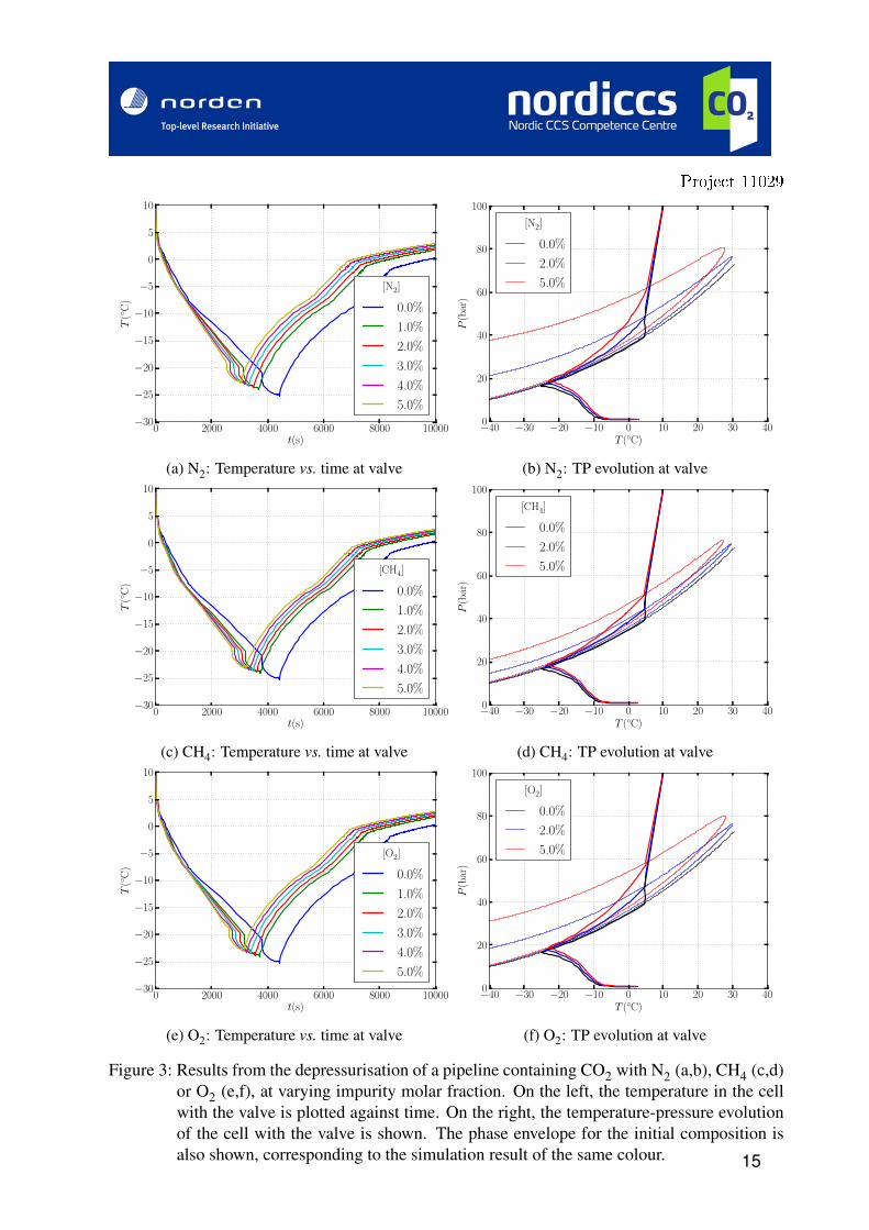
Simulations were performed on the depressurisation of a pipeline containing CO2 with N2, CH4or O2 as the impurity. A valve area of 50cm2 was used. The results, presented in Fig. 3, focus onthe evolution of the thermodynamic state in the computational cell containing the valve, which iswhere the lowest temperatures are reached. From these results, one may find the lowest tempera-ture occurring throughout a simulation. How this value depends on impurity kind and fraction isshown in Fig. 4.
5.3 Effect of valve opening
Simulations were performed on the depressurisation of a pipeline containing 2 mol% N2, witha variable valve opening area. The results are presented in Fig. 5 and 6, similarly focusing onthe thermodynamic state of the cell containing the valve. Note in Fig. 5a how there are somenumerical instabilities in the later parts of the simulations when the valve area becomes verylarge. These may likely be removed by reducing the cell size and time steps further.
13
Project 11029Project 11029
−40 −30 −20 −10 0 10 20 30 40T (◦C)
0
20
40
60
80
100
P(b
ar)
0.00 min
0.33 min
9.67 min
47.00 min
106.00 min
0.00 min
6.00 min
32.33 min
65.00 min
110.33 min
x ≈ 0 m
x ≈ 10 km
(a) Temperature-pressure evolution
0 2000 4000 6000 8000 10000x (m)
−25
−20
−15
−10
−5
0
5
10
T(◦
C)
0.33 min
6.00 min
47.00 min
65.00 min
100.00 min
(b) Temperature
0 2000 4000 6000 8000 10000x (m)
0.0
0.2
0.4
0.6
0.8
1.0
αg(−
)
0.33 min
6.00 min
47.00 min
65.00 min
(c) Gas volume fraction
0 2000 4000 6000 8000 10000x (m)
2.0
2.5
3.0
3.5
4.0
4.5
5.0
5.5
6.0
mol
%N
2(-
)
0.33 min
6.00 min
47.00 min
65.00 min
100.00 min
(d) Overall impurity molar fraction
Figure 2: A closer look at the case of 5 mol% N2 and a 50 cm2 valve opening. The first figure(a) shows the temperature-pressure evolution at the pipeline end by the valve (blueline) and at the opposite end of the valve (red line), together with the phase envelopecorresponding to the initial composition. The temperature, gas volume fraction andaverage composition profiles along the pipeline at a selection of the times in (a) areshown in (b), (c) and (d), respectively.
14
Project 11029Project 11029
0 2000 4000 6000 8000 10000t(s)
−30
−25
−20
−15
−10
−5
0
5
10
T(◦
C)
[N2]
0.0%
1.0%
2.0%
3.0%
4.0%
5.0%
(a) N2: Temperature vs. time at valve
−40 −30 −20 −10 0 10 20 30 40T (◦C)
0
20
40
60
80
100
P(b
ar)
[N2]
0.0%
2.0%
5.0%
(b) N2: TP evolution at valve
0 2000 4000 6000 8000 10000t(s)
−30
−25
−20
−15
−10
−5
0
5
10
T(◦
C)
[CH4]
0.0%
1.0%
2.0%
3.0%
4.0%
5.0%
(c) CH4: Temperature vs. time at valve
−40 −30 −20 −10 0 10 20 30 40T (◦C)
0
20
40
60
80
100
P(b
ar)
[CH4]
0.0%
2.0%
5.0%
(d) CH4: TP evolution at valve
0 2000 4000 6000 8000 10000t(s)
−30
−25
−20
−15
−10
−5
0
5
10
T(◦
C)
[O2]
0.0%
1.0%
2.0%
3.0%
4.0%
5.0%
(e) O2: Temperature vs. time at valve
−40 −30 −20 −10 0 10 20 30 40T (◦C)
0
20
40
60
80
100
P(b
ar)
[O2]
0.0%
2.0%
5.0%
(f) O2: TP evolution at valve
Figure 3: Results from the depressurisation of a pipeline containing CO2 with N2 (a,b), CH4 (c,d)or O2 (e,f), at varying impurity molar fraction. On the left, the temperature in the cellwith the valve is plotted against time. On the right, the temperature-pressure evolutionof the cell with the valve is shown. The phase envelope for the initial composition isalso shown, corresponding to the simulation result of the same colour. 15
Project 11029Project 11029
0 1 2 3 4 5Impurity concentration (mol%)
−25.5
−25.0
−24.5
−24.0
−23.5
−23.0
−22.5
Tm
in(◦
C)
N2
CH4
O2
(a)
0.0 0.5 1.0 1.5 2.0 2.5 3.0 3.5 4.0Impurity concentration (mass%)
−25.5
−25.0
−24.5
−24.0
−23.5
−23.0
−22.5
Tm
in(◦
C)
N2
CH4
O2
(b)
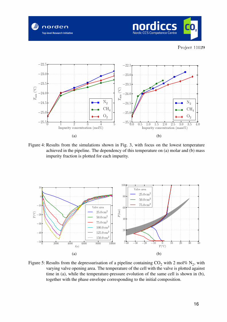
Figure 4: Results from the simulations shown in Fig. 3, with focus on the lowest temperatureachieved in the pipeline. The dependency of this temperature on (a) molar and (b) massimpurity fraction is plotted for each impurity.
0 2000 4000 6000 8000 10000t(s)
−50
−40
−30
−20
−10
0
10
T(◦
C)
Valve area
25.0 cm2
50.0 cm2
75.0 cm2
100.0 cm2
125.0 cm2
150.0 cm2
(a)
−40 −30 −20 −10 0 10 20 30 40T (◦C)
0
20
40
60
80
100
P(b
ar)
Valve area
25.0 cm2
50.0 cm2
75.0 cm2
(b)
Figure 5: Results from the depressurisation of a pipeline containing CO2 with 2 mol% N2, withvarying valve opening area. The temperature of the cell with the valve is plotted againsttime in (a), while the temperature-pressure evolution of the same cell is shown in (b),together with the phase envelope corresponding to the initial composition.
16
Project 11029Project 11029
20 40 60 80 100 120 140 160Valve area (cm2)
−50
−45
−40
−35
−30
−25
−20
−15
−10
Tm
in(◦
C)
[N2]
0.0%
1.0%
2.0%
3.0%
4.0%
5.0%
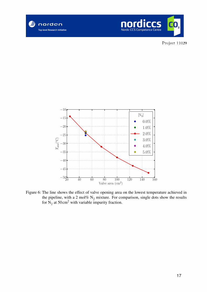
Figure 6: The line shows the effect of valve opening area on the lowest temperature achieved inthe pipeline, with a 2 mol% N2 mixture. For comparison, single dots show the resultsfor N2 at 50cm2 with variable impurity fraction.
17
Project 11029Project 11029
6 Discussion
With regards to the effect of impurities, from studying the results presented in Fig. 3 and 4 onemay claim the following:
• The presence of volatile gas impurities increases the lowest temperature reached, but to avery small degree (no more than about 2◦C for molar fractions up to 5%).
• The presence of volatile gas impurities increases the rate of the temperature drop slightly.
• It does not seem to matter which of these impurities is present, especially when comparingthem by molar fraction.
With regards to the effect of valve opening area, the results in Fig. 5 imply that:
• Increasing the valve area decreases the lowest temperature reached dramatically. In theregion of 50cm2, the lowest temperature decreases by approximately 10◦C per centimetreof increased radius of a circular opening.
• Increasing the valve area also dramatically increases the rate of temperature drop.
Altogether it appears that the effect of the volatile gas impurities on the temperature drop isnegligible compared to the effect of reasonable variations in valve opening area. The two effectsare compared in Fig. 6 for the case of N2 as the impurity.
7 Conclusions
It appears that the presence of volatile gas impurities, here exemplified by N2, CH4 and O2, doesnot make the risk of reaching too low temperatures more severe during CO2 pipeline depressurisa-tion. On the contrary, their presence seems to slightly increase the lowest temperature experiencedin the pipeline. However, their presence increases the rate of temperature decrease slightly. Addi-tionally, it seems that the depressurisation behaviour changes very little when switching betweendifferent kinds of volatile gas impurities.
On the other hand, the valve opening appears to have a major effect on the temperatures reachedand the rate at which it decreases, with a larger opening causing lower temperatures and fasterdrop. In the case of intentional and controlled depressurisation, this implies that any worriesregarding an increased magnitude or rate of temperature drop due to other parameters may likelybe remedied by a slight decrease in the valve opening, if an increase in total time required toempty the pipeline is acceptable.
Note that this does not mean that the presence if volatile gas impurities should be ignored.These imputities significantly enlarge the two-phase area in temperature-pressure space, com-pared to pure CO2. This means that the risk of initiating two-phase flow during pipeline opera-tion is increased, as indicated in [3], something which may introduce many other challenges andpotential problems in addition to temperature drops.
18
Project 11029Project 11029
7.1 Suggestions for further work
Keep in mind that this work only covered a sub-set of the possible impurities which may bepresent in CO2 from capture processes. It remains to be seen how other much less volatile im-purities such as NOx, SOx, H2S and H2O will affect the temperature drop. The latter two are ofparticular interest, since they may separate into their own liquid phase in addition to a CO2-richliquid phase, introducing severe corrosion issues. These impurities present considerable addi-tional challenges for the thermodynamic algorithms, an issue which must be resolved before asimilar study of two-phase flow can be performed with such mixtures. Further work could alsoattempt to study mixtures of more than two components at once, or attempt to vary other parame-ters than composition and valve, such as initial pressure, pipeline radius, heat transfer conditions,etc.
References
[1] J. Capelle et al. “Design based on ductile–brittle transition temperature for API 5L X65steel used for dense CO2 transport”. In: Engineering Fracture Mechanics 110.0 (2013),pp. 270 –280.
[2] P. Aursand et al. “Pipeline transport of CO2 mixtures: Models for transient simulation”.In: International Journal of Greenhouse Gas Control 15.0 (2013), pp. 174 –185.
[3] Alexandre Morin. Dynamic flow of CO2 in pipelines: Sensitivity to impurities. NORDICCSMemo D5.2.1301. SINTEF Energy Research, 2013.
[4] Pedro José Martínez Ferrer, Tore Flåtten, and Svend Tollak Munkejord. “On the effect oftemperature and velocity relaxation in two-phase flow models”. In: ESAIM: MathematicalModelling and Numerical Analysis 46.02 (2012), pp. 411–442.
[5] Giorgio Soave. “Equilibrium constants from a modified Redlich-Kwong equation of state”.In: Chemical engineering science 27.6 (1972), pp. 1197–1203.
[6] TY Kwak and GA Mansoori. “Van der Waals mixing rules for cubic equations of state. Ap-plications for supercritical fluid extraction modelling”. In: Chemical engineering science41.5 (1986), pp. 1303–1309.
[7] J. F. Ely and H. J. M. Hanley. “Prediction of Transport Properties. 1. Viscosity of fluidsand mixtures”. In: Industrial & Engineering Chemistry Fundamentals 20.4 (Nov. 1981),pp. 323–332.
[8] J. F. Ely and H. J. M. Hanley. “Prediction of Transport Properties. 2. Thermal conductivityof pure fluids and mixtures”. In: Industrial & Engineering Chemistry Fundamentals 22.1(Feb. 1983), pp. 90–97.
[9] Eleuterio F. Toro. Riemann solvers and numerical methods for fluid dynamics. Second.Berlin: Springer-Verlag, 1999. ISBN: 3-540-65966-8.
[10] Svend Tollak Munkejord, Steinar Evje, and Tore FlÅtten. “A MUSTA scheme for a non-conservative two-fluid model”. In: SIAM Journal on Scientific Computing 31.4 (2009),pp. 2587–2622.
19

Project 11029Project 11029
[11] Adrian Bejan. Heat Transfer. New York: John Wiley & Sons, Inc., 1993. ISBN: 0-471-50290-1.
[12] Skjalg E. Haaland. “Simple and explicit formulas for the friction factor in turbulent pipeflow”. In: Journal of Fluids Engineering – Transactions of the ASME 105 (1983), pp. 89–90.
[13] PL Spedding and NP Hand. “Prediction in stratified gas-liquid co-current flow in horizontalpipelines”. In: International journal of heat and mass transfer 40.8 (1997), pp. 1923–1935.
20