Embed Size (px)
Citation preview
Dynamic Causal Modelling (DCM) for fMRI
Rosalyn Moran
Virginia Tech Carilion Research Institute
With thanks to the FIL Methods Groupfor slides and images
SPM Course, UCL May 2013
Dynamic causal modelling (DCM)
• DCM framework was introduced in 2003 for fMRI by Karl Friston, Lee Harrison and Will Penny (NeuroImage 19:1273-1302)
• part of the SPM software package
• currently more than 160 published papers on DCM250
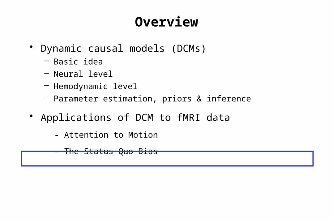
Overview
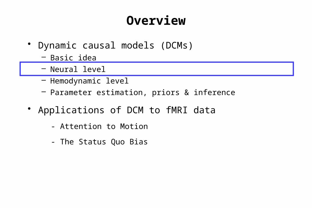
• Dynamic causal models (DCMs)– Basic idea– Neural level– Hemodynamic level– Parameter estimation, priors & inference
• Applications of DCM to fMRI data
- Attention to Motion
- The Status Quo Bias
Overview
• Dynamic causal models (DCMs)– Basic idea– Neural level– Hemodynamic level– Parameter estimation, priors & inference
• Applications of DCM to fMRI data
- Attention to Motion
- The Status Quo Bias
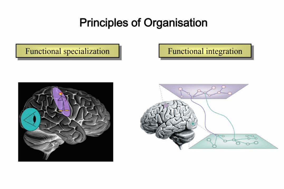
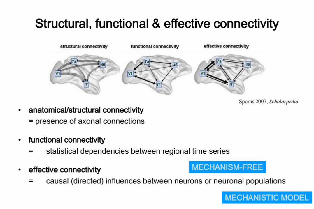
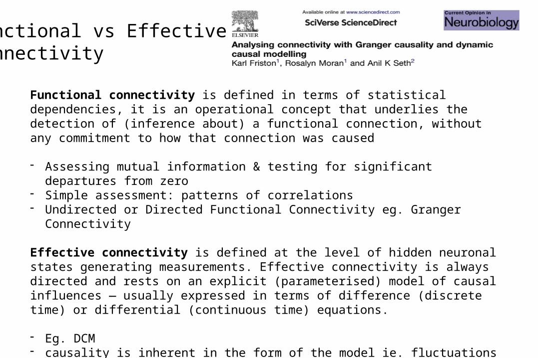
Functional vs Effective Connectivity
Functional connectivity is defined in terms of statistical dependencies, it is an operational concept that underlies the detection of (inference about) a functional connection, without any commitment to how that connection was caused
- Assessing mutual information & testing for significant departures from zero- Simple assessment: patterns of correlations- Undirected or Directed Functional Connectivity eg. Granger Connectivity
Effective connectivity is defined at the level of hidden neuronal states generating measurements. Effective connectivity is always directed and rests on an explicit (parameterised) model of causal influences — usually expressed in terms of difference (discrete time) or differential (continuous time) equations.
- Eg. DCM- causality is inherent in the form of the model ie. fluctuations in hidden neuronal states
cause changes in others: for example, changes in postsynaptic potentials in one area are caused by inputs from other areas.
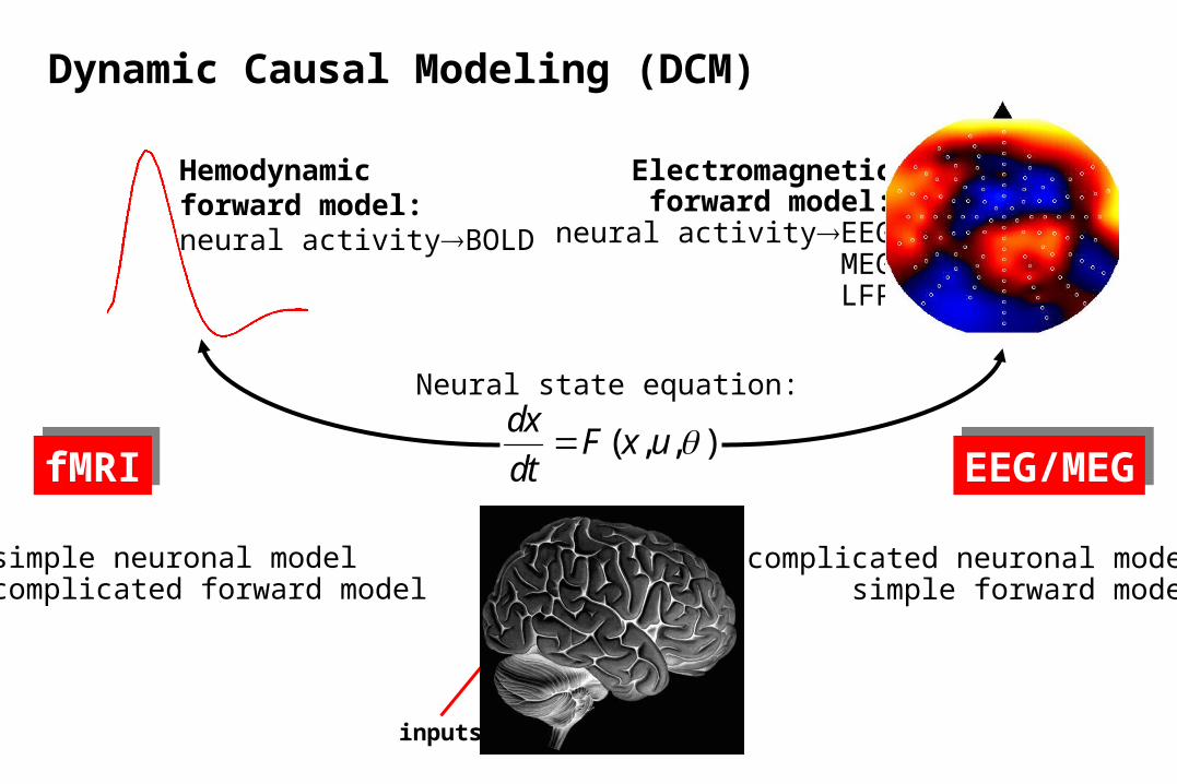
),,( uxFdt
dx
Neural state equation:
Electromagneticforward model:
neural activityEEGMEGLFP
Dynamic Causal Modeling (DCM)
simple neuronal modelcomplicated forward model
complicated neuronal modelsimple forward model
fMRIfMRI EEG/MEGEEG/MEG
inputs
Hemodynamicforward model:neural activityBOLD
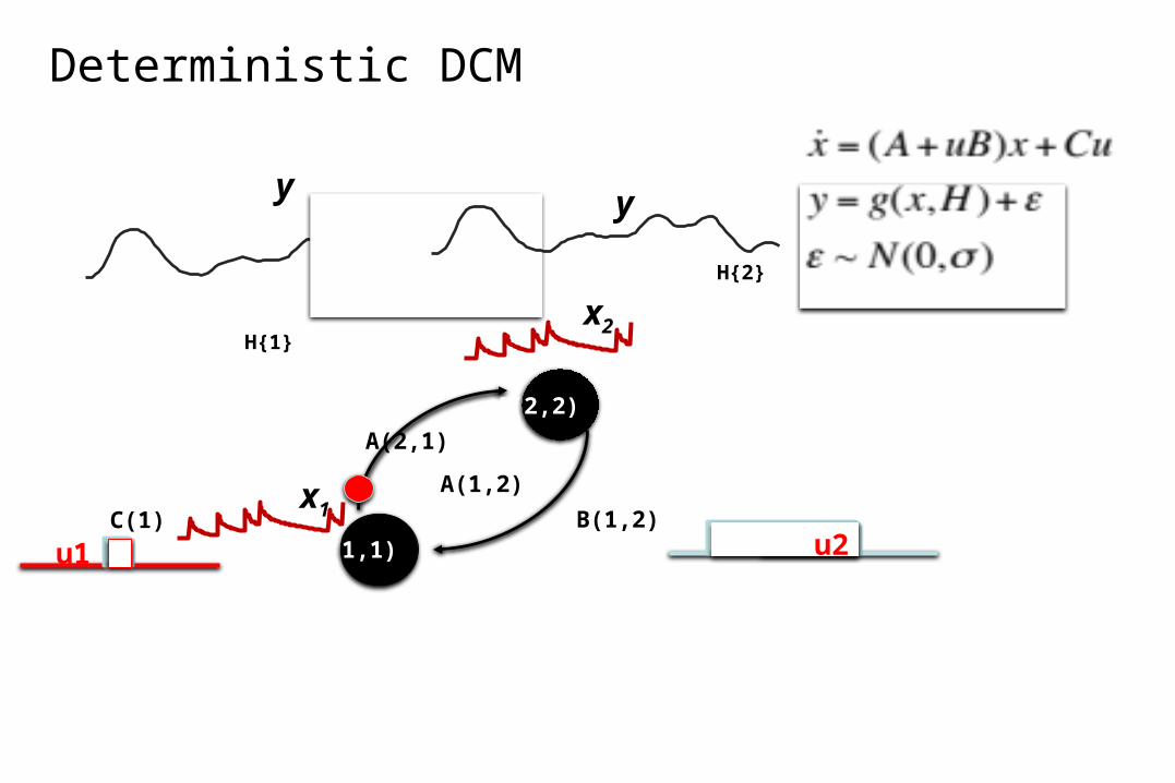
Deterministic DCM
u1 A(1,1)
A(2,1)
A(1,2)
A(2,2)
x1u2
B(1,2)
H{1}
y
H{2}
y
x2
C(1)
Overview
• Dynamic causal models (DCMs)– Basic idea– Neural level– Hemodynamic level– Parameter estimation, priors & inference
• Applications of DCM to fMRI data
- Attention to Motion
- The Status Quo Bias
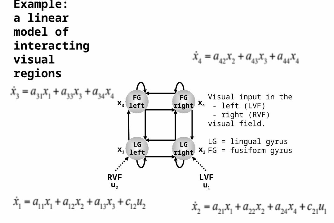
LGleft
LGright
RVF LVF
FGright
FGleft
Visual input in the - left (LVF) - right (RVF)visual field.
LG = lingual gyrusFG = fusiform gyrusx1 x2
x4x3
u2 u1
Example: a linear model of interacting visual regions
LGleft
LGright
RVF LVF
FGright
FGleft
LG = lingual gyrusFG = fusiform gyrus
Visual input in the - left (LVF) - right (RVF)visual field.x1 x2
x4x3
u2 u1
Example: a linear model of interacting visual regions
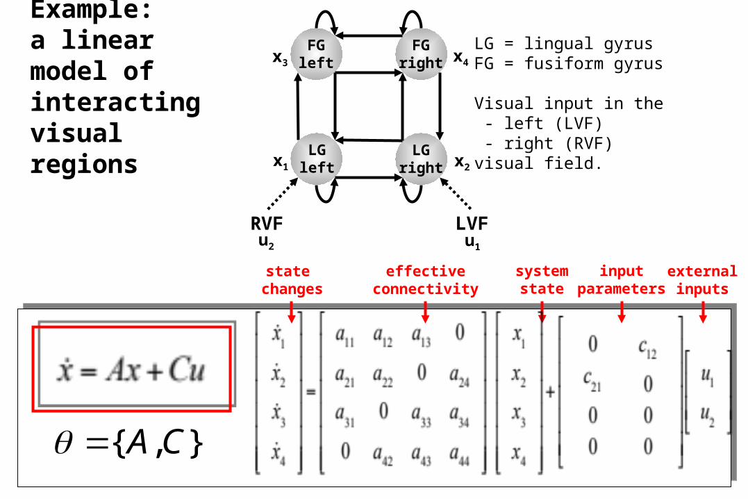
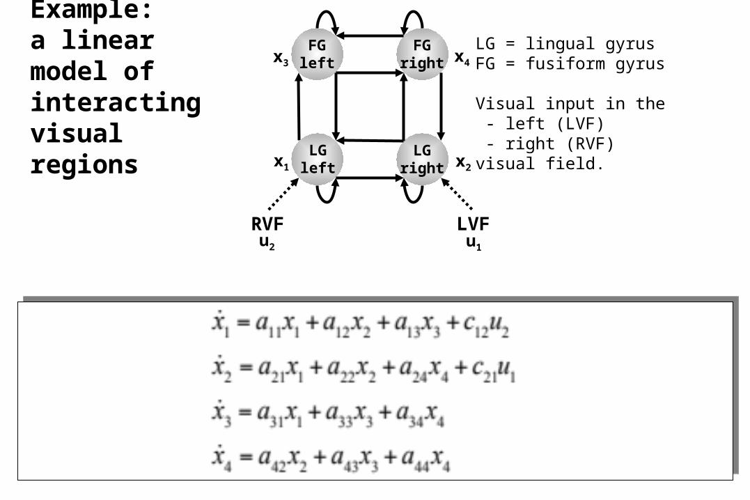
Example: a linear model of interacting visual regions
LG = lingual gyrusFG = fusiform gyrus
Visual input in the - left (LVF) - right (RVF)visual field.
state changes
effectiveconnectivity
externalinputs
systemstate
inputparameters
},{ CA
LGleft
LGright
RVF LVF
FGright
FGleft
x1 x2
x4x3
u2 u1
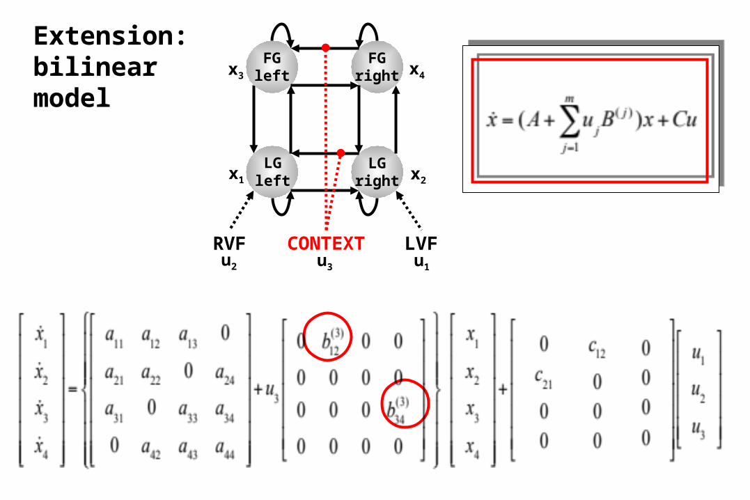
Extension: bilinear model
LGleft
LGright
RVF LVF
FGright
FGleft
x1 x2
x4x3
u2 u1
CONTEXTu3
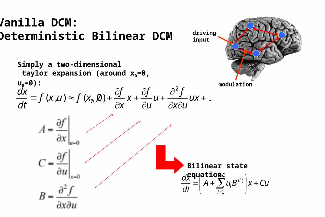
Vanilla DCM:Deterministic Bilinear DCM
CuxBuAdt
dx m
i
ii
1
)(
Bilinear state equation:
driving input
modulation
...)0,(),(2
0
uxux
fu
u
fx
x
fxfuxf
dt
dx
Simply a two-dimensional taylor expansion (around x0=0, u0=0):
-
x2
stimuliu1
contextu2
x1
+
+
-
-
-+ u1
Z1
u2
Z2
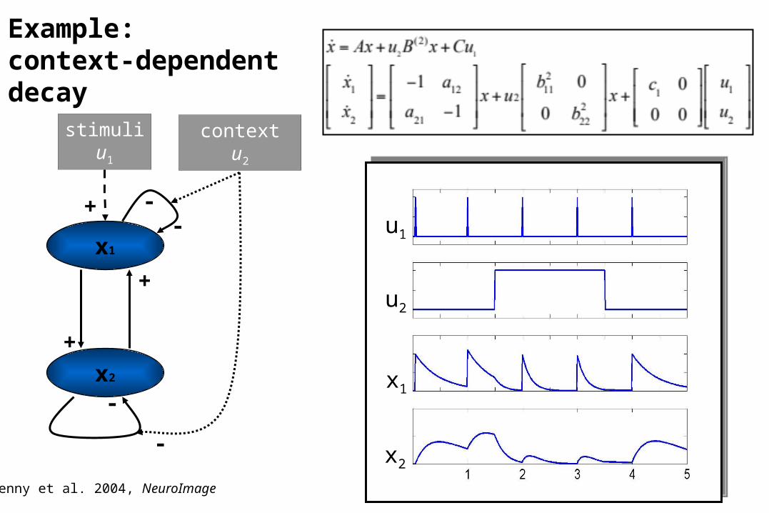
Example: context-dependent decay
u1
u2
x2
x1
Penny et al. 2004, NeuroImage
+
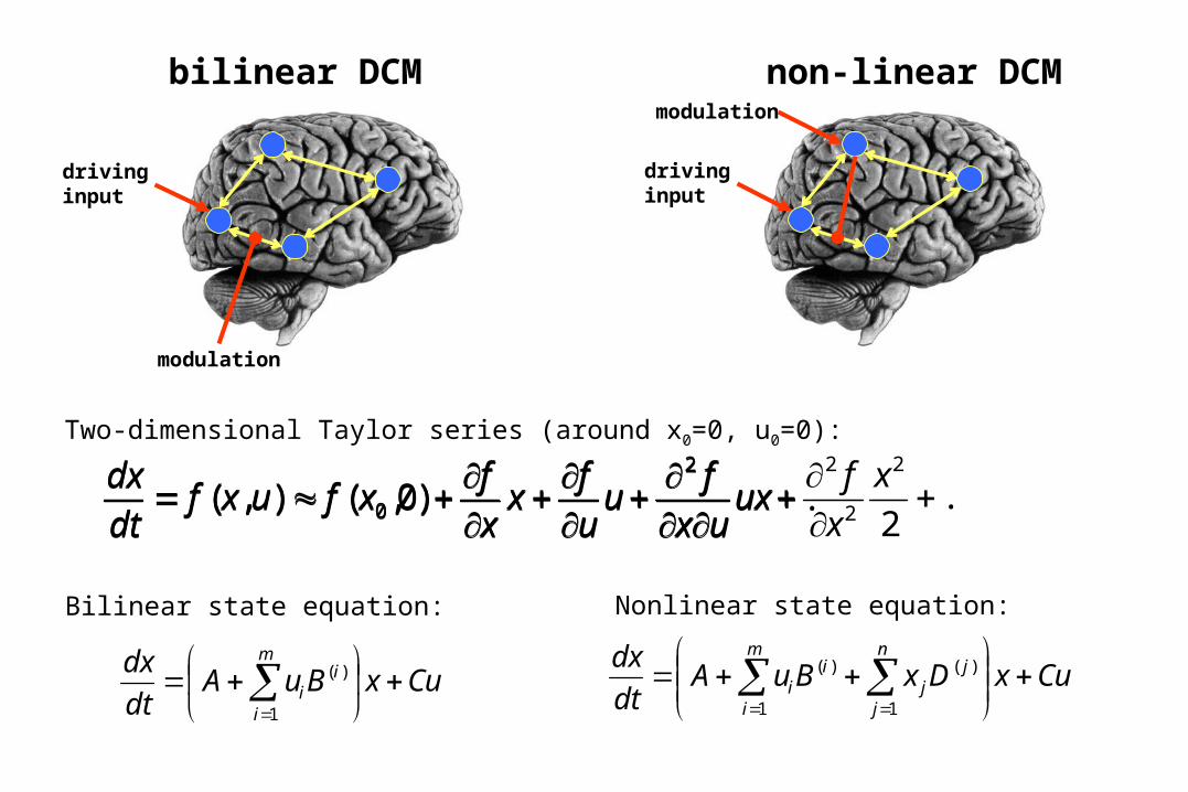
bilinear DCM
CuxDxBuAdt
dx m
i
n
j
jj
ii
1 1
)()(CuxBuA
dt
dx m
i
ii
1
)(
Bilinear state equation:
driving input
modulation
driving input
modulation
non-linear DCM
...)0,(),(2
0
uxux
fu
u
fx
x
fxfuxf
dt
dx
Two-dimensional Taylor series (around x0=0, u0=0):
Nonlinear state equation:
...2
)0,(),(2
2
22
0
x
x
fux
ux
fu
u
fx
x
fxfuxf
dt
dx
0 10 20 30 40 50 60 70 80 90 100
0
0.1
0.2
0.3
0.4
0 10 20 30 40 50 60 70 80 90 100
0
0.2
0.4
0.6
0 10 20 30 40 50 60 70 80 90 100
0
0.1
0.2
0.3
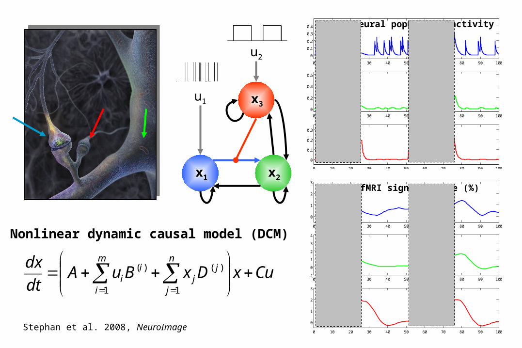
Neural population activity
0 10 20 30 40 50 60 70 80 90 100
0
1
2
3
0 10 20 30 40 50 60 70 80 90 100-1
0
1
2
3
4
0 10 20 30 40 50 60 70 80 90 100
0
1
2
3
fMRI signal change (%)
x1 x2
x3
CuxDxBuAdt
dx n
j
jj
m
i
ii
1
)(
1
)(
Nonlinear dynamic causal model (DCM)
Stephan et al. 2008, NeuroImage
u1
u2
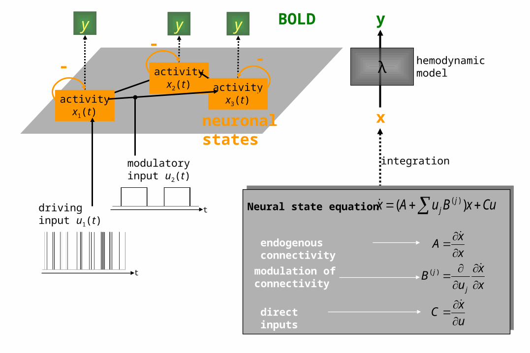
endogenous connectivity
direct inputs
modulation ofconnectivity
Neural state equation CuxBuAx jj )( )(
u
xC
x
x
uB
x
xA
j
j
)(
hemodynamicmodelλ
x
y
integration
BOLDyyy
activityx1(t)
activityx2(t) activity
x3(t)
neuronalstates
t
drivinginput u1(t)
modulatoryinput u2(t)
t
Overview
• Dynamic causal models (DCMs)– Basic idea– Neural level– Hemodynamic level– Parameter estimation, priors & inference
• Applications of DCM to fMRI data
- Attention to Motion
- The Status Quo Bias
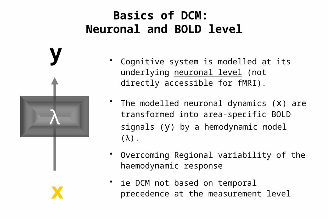
• Cognitive system is modelled at its underlying neuronal level (not directly accessible for fMRI).
• The modelled neuronal dynamics (x) are transformed into area-specific BOLD signals
(y) by a hemodynamic model (λ).
• Overcoming Regional variability of the haemodynamic response
• ie DCM not based on temporal precedence at the measurement level
λ
x
y
Basics of DCM: Neuronal and BOLD level
λ
x
y
Basics of DCM: Neuronal and BOLD level
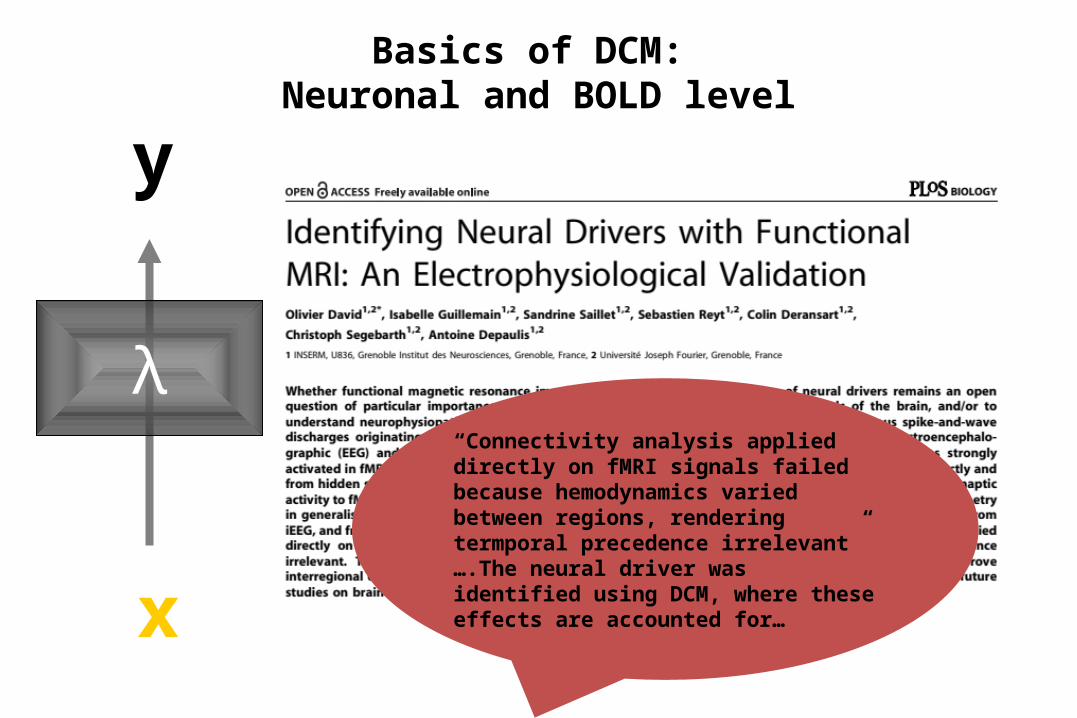
“Connectivity analysis applied directly on fMRI signals failed because hemodynamics varied between regions, rendering termporal precedence irrelevant” ….The neural driver was identified using DCM, where these effects are accounted for…
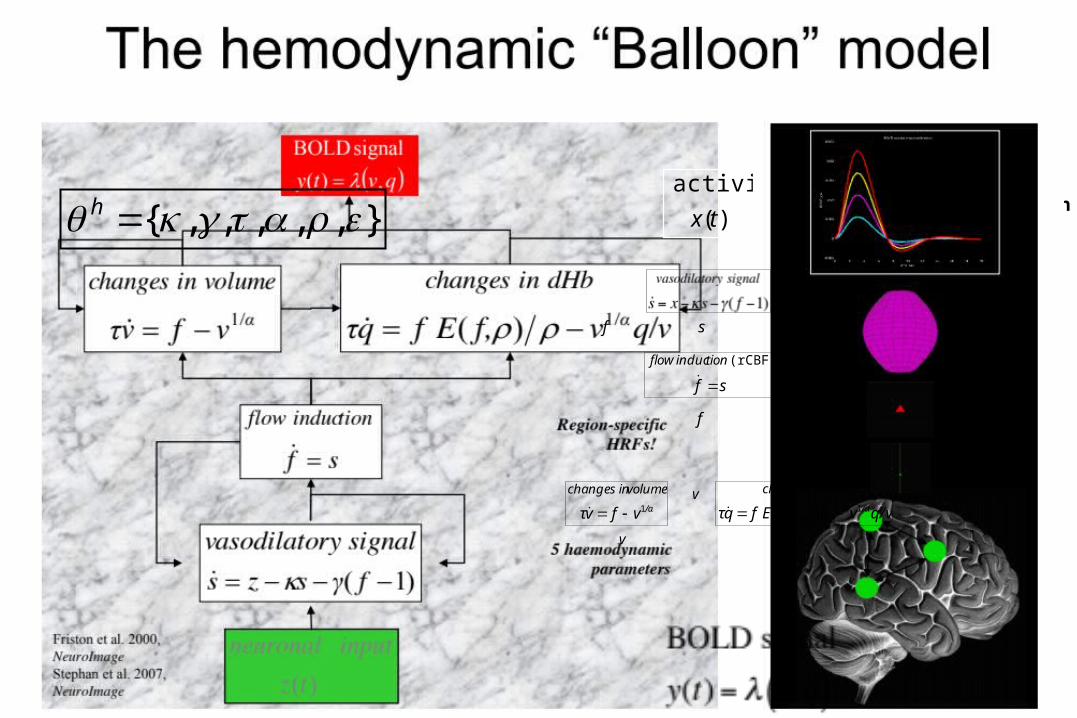
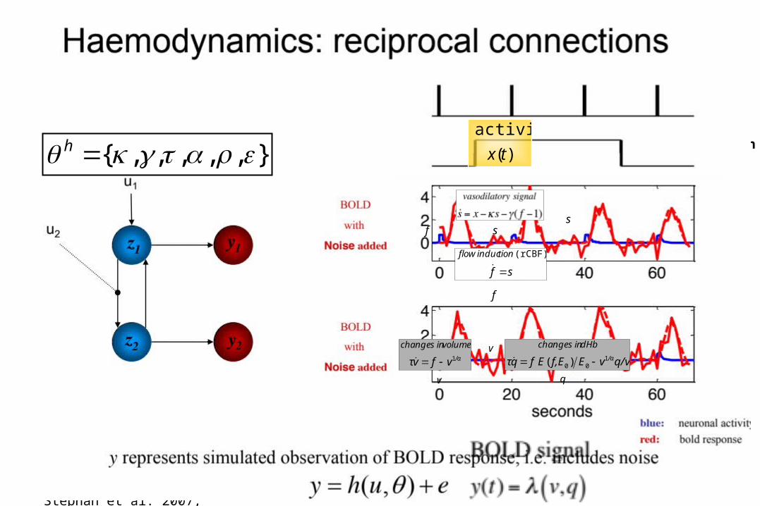
},,,,,{ h
important for model fitting, but of no interest for statistical inference
The hemodynamic model
)(
activity
tx
• 6 hemodynamic parameters:
• Computed separately for each area region-specific HRFs!
sf
tionflow induc
(rCBF)
s
v
v
q q/vvEf,EEfqτ /α
dHbchanges in
100 )( /αvfvτ
volumechanges in
1
f
q
s
f
Friston et al. 2000, NeuroImageStephan et al. 2007, NeuroImage
stimulus functionsut
neural state equation
hemodynamic state equations
Estimated BOLD response
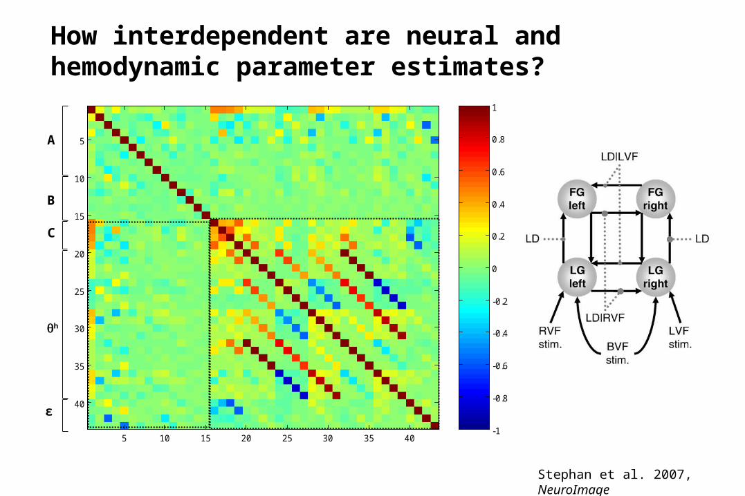
5 10 15 20 25 30 35 40
5
10
15
20
25
30
35
40
-1
-0.8
-0.6
-0.4
-0.2
0
0.2
0.4
0.6
0.8
1
A
B
C
h
ε
How interdependent are neural and hemodynamic parameter estimates?
Stephan et al. 2007, NeuroImage
Overview
• Dynamic causal models (DCMs)– Basic idea– Neural level– Hemodynamic level– Parameter estimation, priors & inference
• Applications of DCM to fMRI data
- Attention to Motion
- The Status Quo Bias
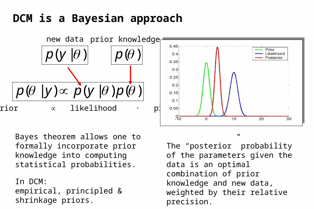
DCM is a Bayesian approach
)()|()|( pypyp posterior likelihood ∙ prior
)|( yp )(p
Bayes theorem allows one to formally incorporate prior knowledge into computing statistical probabilities.
In DCM: empirical, principled & shrinkage priors.
The “posterior” probability of the parameters given the data is an optimal combination of prior knowledge and new data, weighted by their relative precision.
new data prior knowledge
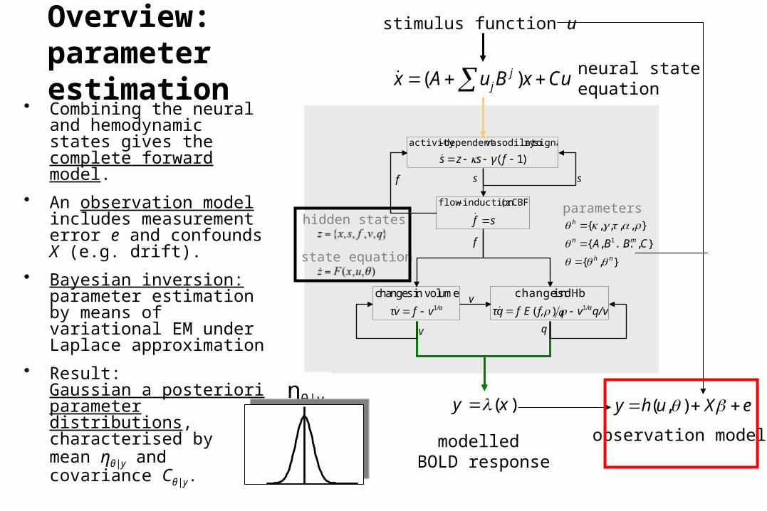
sf (rCBF)induction -flow
s
v
f
stimulus function u
modelled BOLD response
vq q/vvf,Efqτ /α1)(
dHbin changes
/αvfvτ 1
in volume changes
f
q
)1(
signalry vasodilatodependent -activity
fγszs
s
)(xy eXuhy ),(
observation model
hidden states
state equation
parameters
},{
},...,{
},,,,{1
nh
mn
h
CBBA
• Combining the neural and hemodynamic states gives the complete forward model.
• An observation model includes measurement error e and confounds X (e.g. drift).
• Bayesian inversion: parameter estimation by means of variational EM under Laplace approximation
• Result:Gaussian a posteriori parameter distributions, characterised by mean ηθ|y and covariance Cθ|y.
Overview:parameter estimation
ηθ|y
neural stateequation( )j
jx A u B x Cu
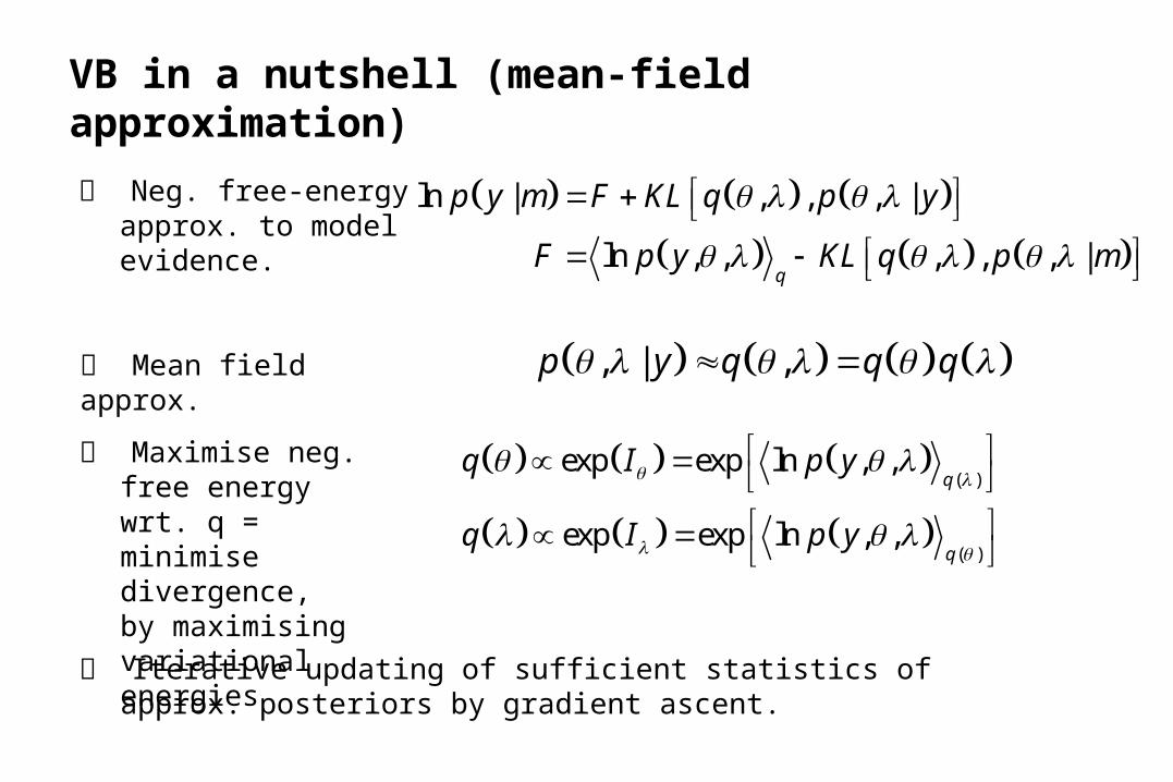
VB in a nutshell (mean-field approximation)
, | ,p y q q q
( )
( )
exp exp ln , ,
exp exp ln , ,
q
q
q I p y
q I p y
Iterative updating of sufficient statistics of approx. posteriors by gradient ascent.
ln | , , , |
ln , , , , , |q
p y m F KL q p y
F p y KL q p m
Mean field approx.
Neg. free-energy approx. to model evidence.
Maximise neg. free energy wrt. q = minimise divergence,by maximising variational energies
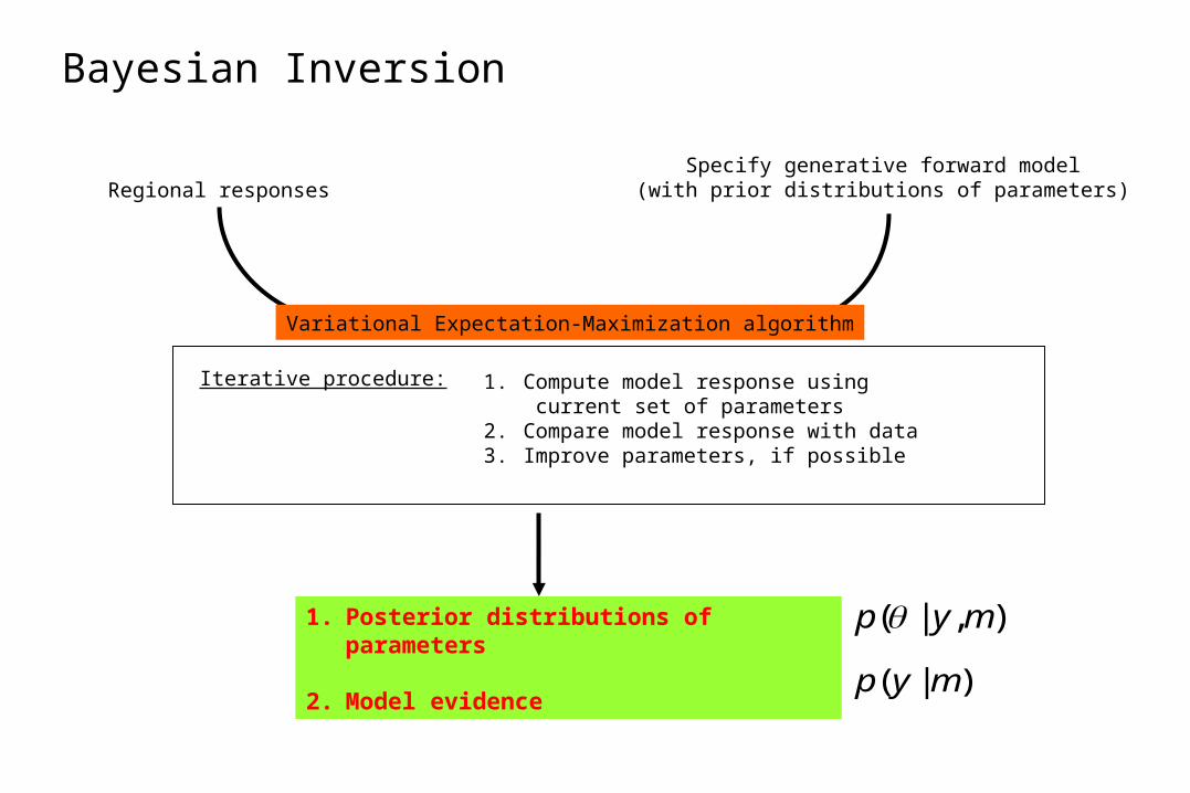
Bayesian Inversion
Regional responsesSpecify generative forward model
(with prior distributions of parameters)
Variational Expectation-Maximization algorithm
Iterative procedure: 1. Compute model response using current set of parameters
2. Compare model response with data3. Improve parameters, if possible
1. Posterior distributions of parameters
2. Model evidence )|( myp
),|( myp
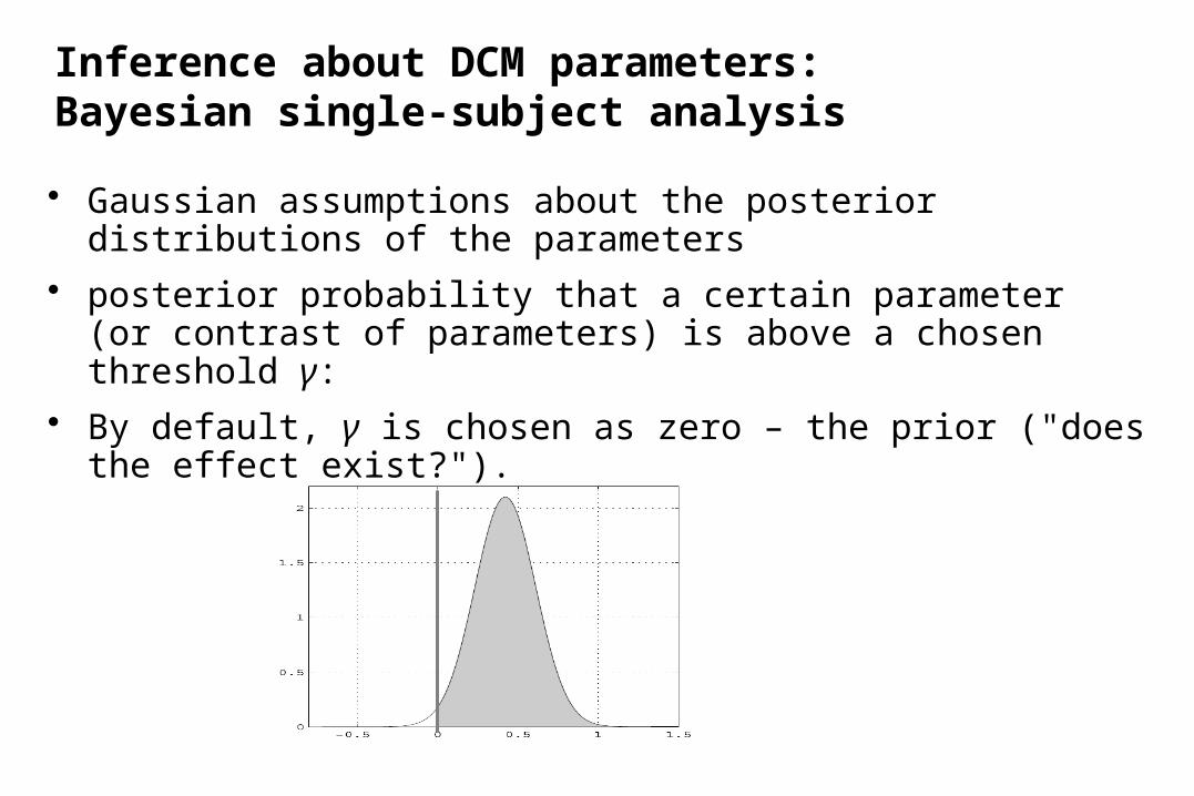
• Gaussian assumptions about the posterior distributions of the parameters
• posterior probability that a certain parameter (or contrast of parameters) is above a chosen threshold γ:
• By default, γ is chosen as zero – the prior ("does the effect exist?").
Inference about DCM parameters:Bayesian single-subject analysis
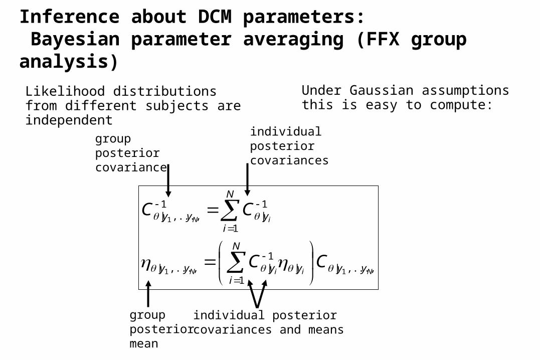
Likelihood distributions from different subjects are independent
NiiN
iN
yy
N
iyyyy
N
iyyy
CC
CC
,...,|1
|1|,...,|
1
1|
1,...,|
11
1
Under Gaussian assumptions this is easy to compute:
groupposterior covariance
individualposterior covariances
groupposterior mean
individual posterior covariances and means
Inference about DCM parameters: Bayesian parameter averaging (FFX group analysis)
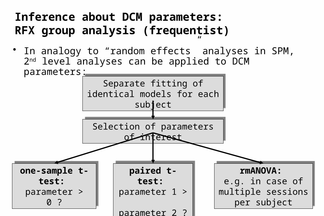
Inference about DCM parameters:RFX group analysis (frequentist)
• In analogy to “random effects” analyses in SPM, 2nd level analyses can be applied to DCM parameters:
Separate fitting of identical models for each subject
Separate fitting of identical models for each subject
Selection of parameters of interest
Selection of parameters of interest
one-sample t-test:
parameter > 0 ?
one-sample t-test:
parameter > 0 ?
paired t-test: parameter 1 > parameter 2 ?
paired t-test: parameter 1 > parameter 2 ?
rmANOVA: e.g. in case of
multiple sessions per subject
rmANOVA: e.g. in case of
multiple sessions per subject
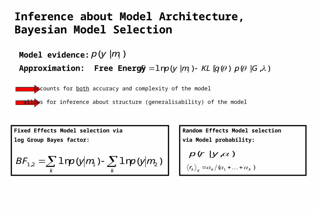
Model evidence:
Approximation: Free Energy
kk
mypmypBF )(ln)(ln 212,1
Fixed Effects Model selection via
log Group Bayes factor:
accounts for both accuracy and complexity of the model
allows for inference about structure (generalisability) of the model
)|( imyp
)],|(),([)|(ln GpqKLmypF i
( | , )p r y
Random Effects Model selection
via Model probability:
)( 1 Kkqkr
Inference about Model Architecture, Bayesian Model Selection
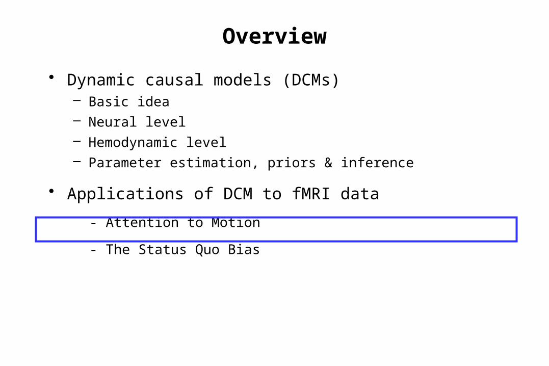
Overview
• Dynamic causal models (DCMs)– Basic idea– Neural level– Hemodynamic level– Parameter estimation, priors & inference
• Applications of DCM to fMRI data
- Attention to Motion
- The Status Quo Bias
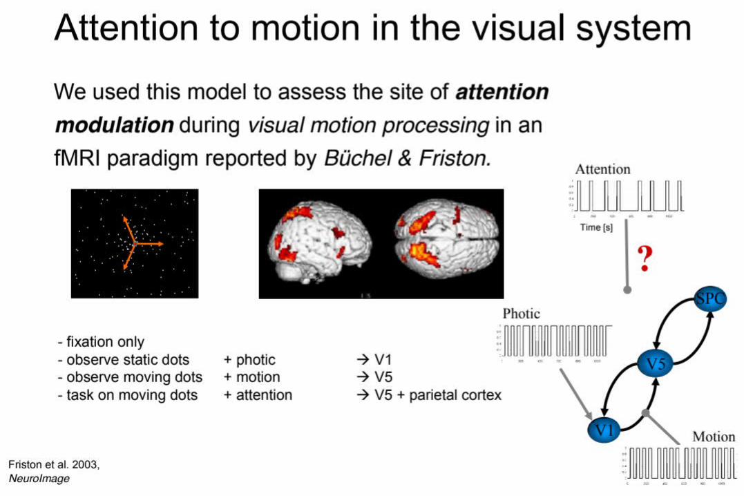
DCM – Attention to MotionParadigm
What connection in the network mediates attention ?
4 conditions
- fixation only baseline- observe static dots + photic
- observe moving dots + motion- attend to moving dots
Bayesian Model Selection
Results
Büchel & Friston 1997, Cereb. CortexBüchel et al. 1998, Brain
V5+
SPCV3A
Attention – No attention
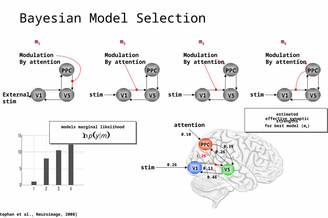
m1 m2
V1 V5stim
PPC
ModulationBy attention
V1 V5Externalstim
PPC
ModulationBy attention
m3
V1 V5stim
PPC
ModulationBy attention
m4
V1 V5stim
PPC
ModulationBy attention
V1 V5stim
PPC
attention
1.25
0.13
0.46
0.39 0.26
0.26
0.10
estimatedeffective synaptic strengths
for best model (m4)
[Stephan et al., Neuroimage, 2008]
models marginal likelihood
ln p y m
Bayesian Model Selection
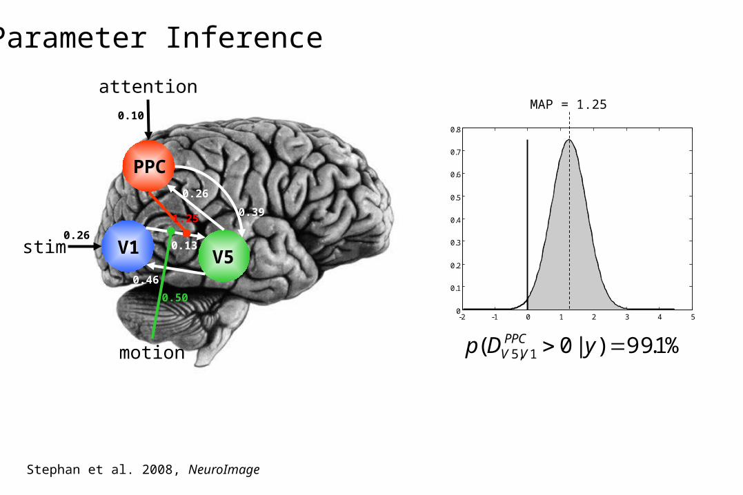
V1 V5stim
PPC
attention
motion
-2 -1 0 1 2 3 4 50
0.1
0.2
0.3
0.4
0.5
0.6
0.7
0.8
%1.99)|0( 1,5 yDp PPCVV
1.25
0.13
0.46
0.39
0.26
0.50
0.26
0.10MAP = 1.25
Stephan et al. 2008, NeuroImage
Parameter Inference
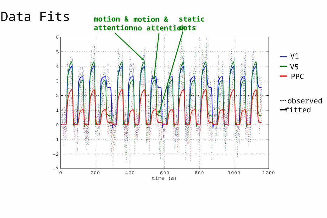
V1
V5PPC
observedfitted
motion &attention
motion &no attention
static dots
Data Fits
Overview
• Dynamic causal models (DCMs)– Basic idea– Neural level– Hemodynamic level– Parameter estimation, priors & inference
• Applications of DCM to fMRI data
- Attention to Motion
- The Status Quo Bias
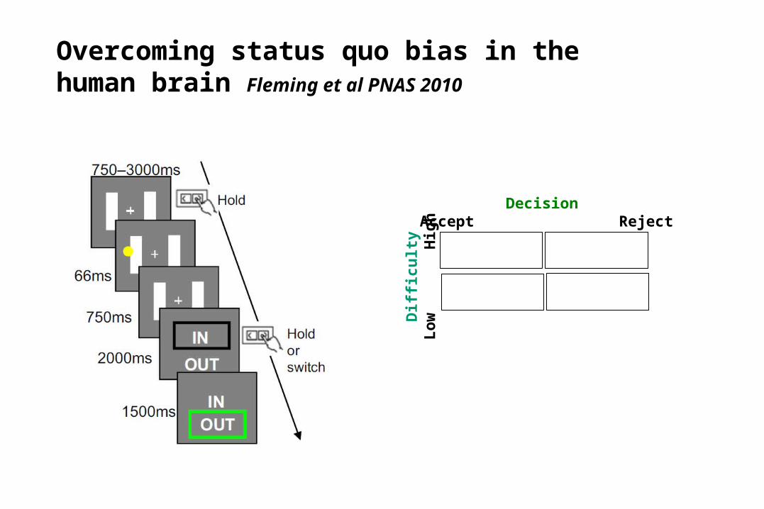
Overcoming status quo bias in the human brain Fleming et al PNAS 2010
Decision Accept Reject
Dif
ficu
lty
Lo
w
H
igh
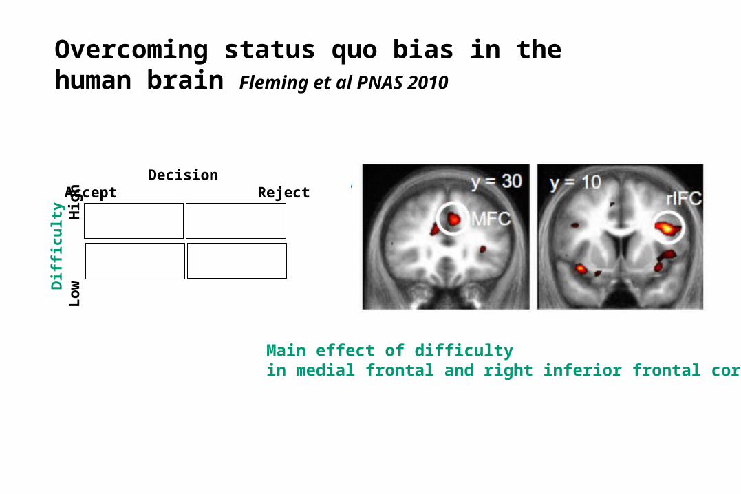
Overcoming status quo bias in the human brain Fleming et al PNAS 2010
Main effect of difficulty in medial frontal and right inferior frontal cortex
Decision Accept Reject
Dif
ficu
lty
Lo
w
H
igh
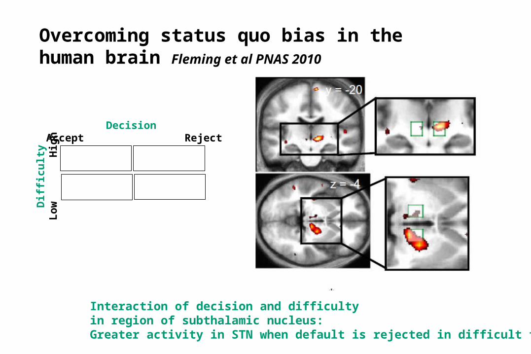
Overcoming status quo bias in the human brain Fleming et al PNAS 2010
Interaction of decision and difficulty in region of subthalamic nucleus:Greater activity in STN when default is rejected in difficult trials
Decision Accept Reject
Dif
ficu
lty
Lo
w
H
igh
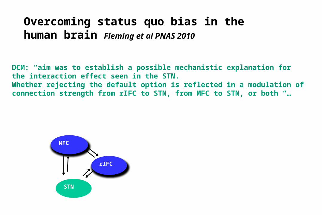
Overcoming status quo bias in the human brain Fleming et al PNAS 2010
DCM: “aim was to establish a possible mechanistic explanation for the interaction effect seen in the STN. Whether rejecting the default option is reflected in a modulation of connection strength from rIFC to STN, from MFC to STN, or both “…
MFC
rIFC
STN
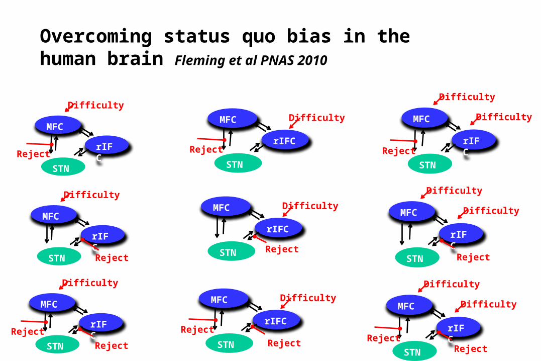
Overcoming status quo bias in the human brain Fleming et al PNAS 2010
MFC
rIFC
STN
Difficulty
Reject
MFC
rIFC
STN
Difficulty
Reject
MFC
rIFC
STN
Difficulty
Difficulty
Reject
MFC
rIFC
STN
Difficulty
Reject
MFC
rIFC
STN
Difficulty
Reject
MFC
rIFC
STN
Difficulty
Difficulty
Reject
MFC
rIFC
STN
Difficulty
Reject
MFC
rIFC
STN
Difficulty
Reject
MFC
rIFC
STN
Difficulty
Difficulty
RejectReject
RejectReject
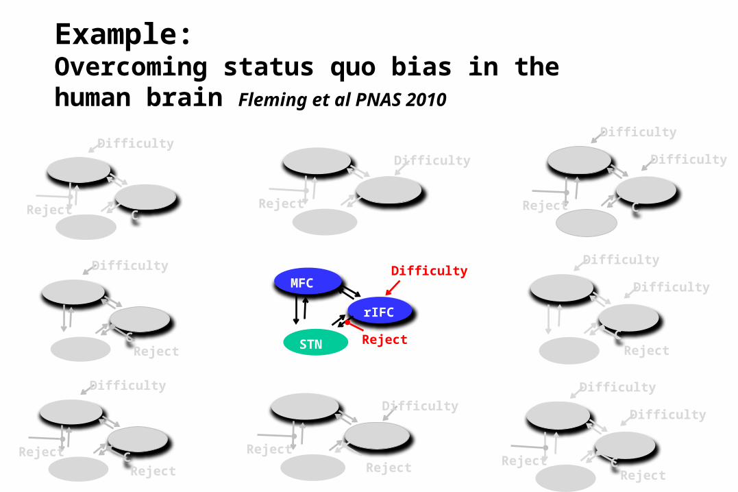
Example:Overcoming status quo bias in the human brain Fleming et al PNAS 2010
MFC
rIFC
STN
Difficulty
Reject
MFC
rIFC
STN
Difficulty
Reject
MFC
rIFC
STN
Difficulty
Difficulty
Reject
MFC
rIFC
STN
Difficulty
Reject
MFC
rIFC
STN
Difficulty
Reject
MFC
rIFC
STN
Difficulty
Difficulty
Reject
MFC
rIFC
STN
Difficulty
Reject
MFC
rIFC
STN
Difficulty
Reject
MFC
rIFC
STN
Difficulty
Difficulty
RejectReject
RejectReject
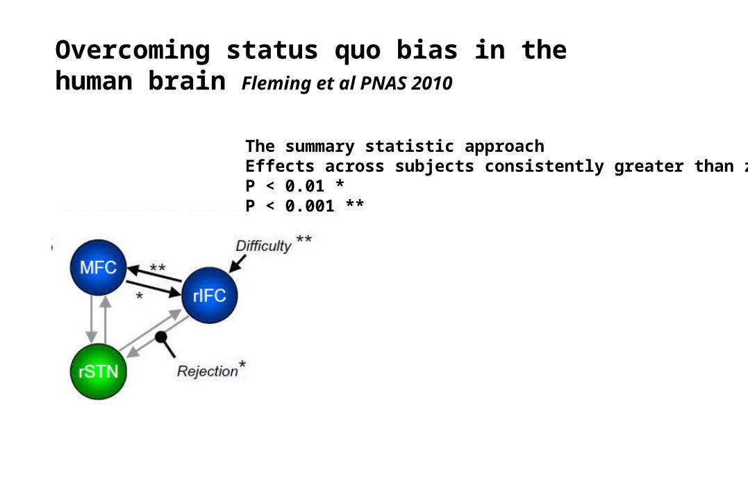
Overcoming status quo bias in the human brain Fleming et al PNAS 2010
The summary statistic approachEffects across subjects consistently greater than zero P < 0.01 *P < 0.001 **
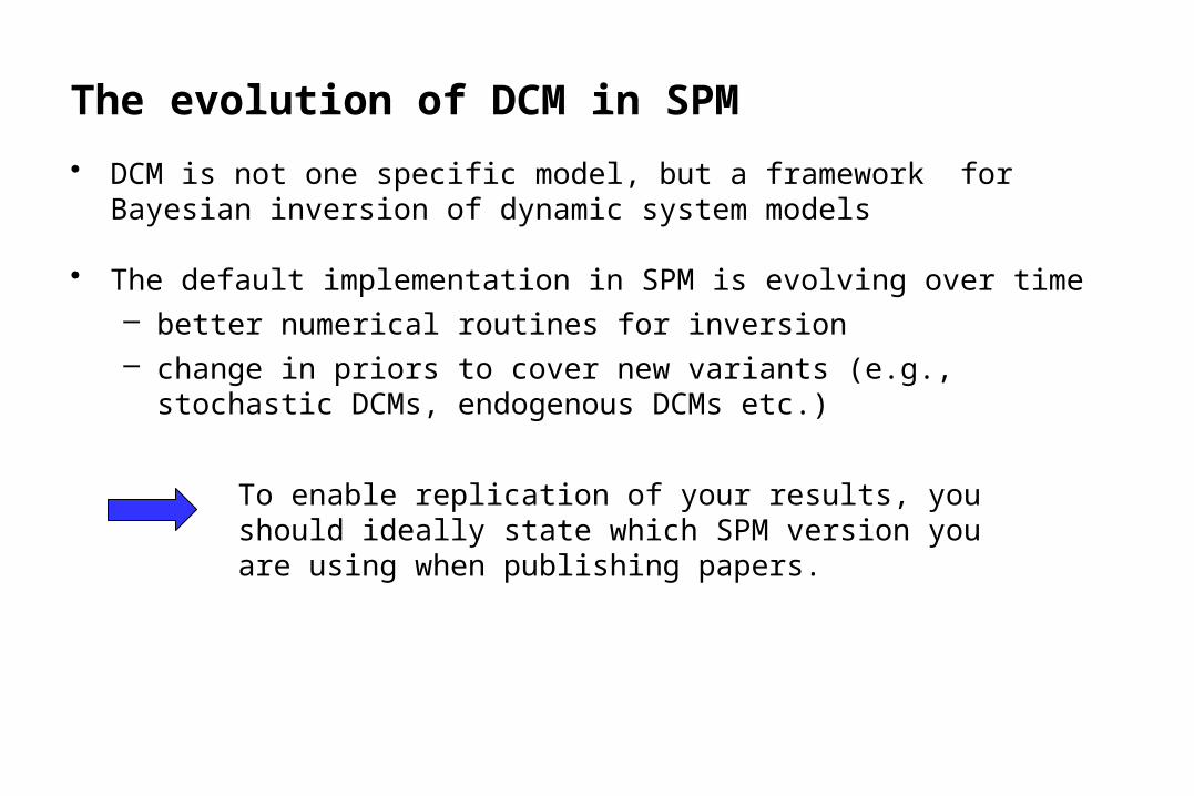
The evolution of DCM in SPM
• DCM is not one specific model, but a framework for Bayesian inversion of dynamic system models
• The default implementation in SPM is evolving over time– better numerical routines for inversion– change in priors to cover new variants (e.g., stochastic DCMs,
endogenous DCMs etc.)
To enable replication of your results, you should ideally state which SPM version you are using when publishing papers.
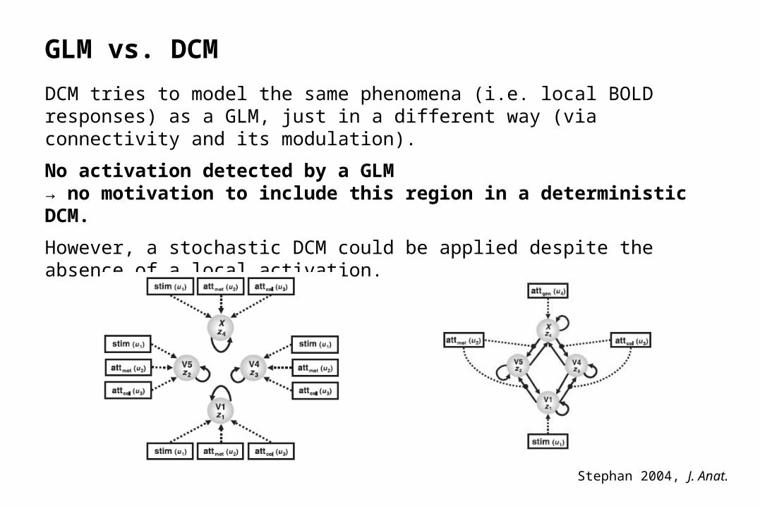
GLM vs. DCM
DCM tries to model the same phenomena (i.e. local BOLD responses) as a GLM, just in a different way (via connectivity and its modulation).
No activation detected by a GLM → no motivation to include this region in a deterministic DCM.
However, a stochastic DCM could be applied despite the absence of a local activation.
Stephan 2004, J. Anat.

Thank you