Embed Size (px)
Citation preview

Digital Object Identifier (DOI) 10.1007/s00220-013-1777-zCommun. Math. Phys. 323, 1017–1070 (2013) Communications in
MathematicalPhysics
Dynamic and Steady States for Multi-DimensionalKeller-Segel Model with Diffusion Exponent m > 0
Shen Bian1,2, Jian-Guo Liu2
1 Department of Mathematical Sciences, Tsinghua University, Beijing, 100084, P.R. China.E-mail: [email protected]
2 Department of Physics and Department of Mathematics, Duke University, Durham, NC 27708, USA.E-mail: [email protected]
Received: 7 June 2012 / Accepted: 1 February 2013Published online: 1 September 2013 – © Springer-Verlag Berlin Heidelberg 2013
Abstract: This paper investigates infinite-time spreading and finite-time blow-up forthe Keller-Segel system. For 0 < m ≤ 2 − 2/d, the L p space for both dynamic andsteady solutions are detected with p := d(2−m)
2 . Firstly, the global existence of theweak solution is proved for small initial data in L p. Moreover, when m > 1 − 2/d,the weak solution preserves mass and satisfies the hyper-contractive estimates in Lq
for any p < q < ∞. Furthermore, for slow diffusion 1 < m ≤ 2 − 2/d, this weaksolution is also a weak entropy solution which blows up at finite time provided by theinitial negative free energy. For m > 2 − 2/d, the hyper-contractive estimates are alsoobtained. Finally, we focus on the L p norm of the steady solutions, it is shown that theenergy critical exponent m = 2d/(d + 2) is the critical exponent separating finite L p
norm and infinite L p norm for the steady state solutions.
1. Introduction
In this paper, we study the Keller-Segel model in spatial dimension d ≥ 3:⎧⎨
⎩
ut = �um − ∇ · (u∇c) , x ∈ Rd , t ≥ 0,
−�c = u, x ∈ Rd , t ≥ 0,
u(x, 0) = U0(x) ≥ 0, x ∈ Rd .
(1.1)
Here the diffusion exponent m is taken to be supercritical 0 < m < 2 − 2/d, criticalmc := 2 − 2/d, and subcritical m > 2 − 2/d. This model is developed to describethe biological phenomenon chemotaxis [30,37]. In the context of biological aggrega-tion, u(x, t) represents the bacteria density, c(x, t) represents the chemical substanceconcentration and it is given by the fundamental solution
c(x, t) = cd
∫
Rd
u(y, t)
|x − y|d−2 dy, (1.2)

1018 S. Bian, J.-G. Liu
where
cd = 1
d(d − 2)αd, αd = πd/2
�(d/2 + 1), (1.3)
αd is the volume of d-dimensional unit ball. The case m < 1 is called fast diffusion andthe case m > 1 is called slow diffusion [14]. The main characteristic of Eq. (1.1) is thecompetition between the diffusion and the nonlocal aggregation. This is well representedby the free energy for m > 1,
F(u) = 1
m − 1
∫
Rdum(x)dx − 1
2
∫
Rduc(x)dx
= 1
m − 1
∫
Rdum(x)dx − cd
2
∫∫
Rd×Rd
u(x)u(y)
|x − y|d−2 dxdy. (1.4)
For m = 1, the first term of the free energy is replaced by∫
Rd u log udx [37]. The com-petition between these two terms leads to finite-time blow-up and infinite time spreading[7–9,13,28,37,40,41]. For the fast diffusion case 0 < m < 1, the free energy becomes
F(u) = −[
1
1 − m
∫
Rdumdx +
1
2
∫
Rd|∇c|2dx
]
, (1.5)
both terms are non-positive and we couldn’t directly see the competition between thediffusion and the aggregation terms.
On the other hand, (1.1) can be recast as
ut = ∇ · (u∇μ), (1.6)
where μ is the chemical potential
μ ={ m
m−1 um−1 − c, m �= 1,log u − c, m = 1.
(1.7)
Indeed μ is the first order variation of F(u), thus multiplying (1.6) by μ and integrationin space one has
d F
dt+∫
Rdu |∇μ|2 dx = 0,
or
d F
dt+∫
Rd
∣∣∣∣
2m
2m − 1∇um− 1
2 − √u∇c
∣∣∣∣
2
dx = 0. (1.8)
This implies that F [u(·, t)] is non-increasing with respect to t . For simplicity, we willuse ‖u‖r = ‖u‖Lr (Rd ) through this paper.
Notice that for d ≥ 3, the PDE (1.1) possesses a scaling invariance which leaves theL p norm invariant and produces a balance between the diffusion and the aggregationterms where
p := d(2 − m)
2∈ [1, d). (1.9)

Dynamic and Steady States for Multi-Dimensional Keller-Segel Model 1019
Indeed, if u(x, t) is a solution, then uλ(x, t) = λu(λ(2−m)/2x, λt
)is also a solution and
this scaling preserves the L p norm ‖uλ‖p = ‖u‖p. For the critical case mc := 2 − 2/d,the above scaling becomes the mass invariant scaling uλ(x, t) = λu
(λ1/d x, λt
). Using
the mass invariant scaling, we have that for the supercritical case m < mc, the aggre-gation dominates the diffusion for high density (large λ) and the density has finite-timeblow-up [8,10,25,26,37,40]. While for low density (small λ), the diffusion dominatesthe aggregation and the density has infinite-time spreading [3,37,40,41]. On the con-trary, for the subcritical case m > mc, the aggregation dominates the diffusion forlow density and prevents spreading, while for high density, the diffusion dominates theaggregation thus blow-up is precluded [31,40,41]. These behaviors also appear in manyother physical systems such as thin film, Hele-Shaw, stellar collapse, etc., and they alsobear some similarities to the nonlinear Schrödinger equation [10,15,45,47].
The system (1.1) has been widely studied recently [2,7–9,13,17,28,31,37,40–42]and the references therein, most of the prior estimates for the Keller-Segel model arebased on the arguments of Jäger and Luckhaus [28] with fast decay at infinity that forany q > 1,
d
dt
∫
Rduq dx = − 4mq(q − 1)
(m + q − 1)2
∫
Rd
∣∣∣∇u(m+q−1)/2
∣∣∣2
dx + (q − 1)∫
Rduq+1dx .
(1.10)
When m > 2 − 2/d, there exists a global weak solution without any restriction onthe initial data [2,40,41]. For radially symmetric and compactly supported initial data,Kim and Yao [31] showed that the solution remains radially symmetric and compactlysupported, and it converges to a compactly supported stationary solution exponentiallywith the same mass. For non-compactly supported radially initial data, it is still unclearwhether all the initial mass are attracted to the steady profile (see Sect. 5.3 for numericalsimulations). When 0 < m ≤ 2 − 2/d, Sugiyama, etc. [40,41] considered more generalcase that the second equation of (1.1) is replaced by −�c + γ c = u, γ ≥ 0 and provedthat for initial data U0 ∈ L1 ∩ L∞(Rd),U m
0 ∈ H1(Rd), 1 < q < ∞, if the initialdata satisfies ‖U0‖p < C , where C is a positive number depending on q, d,m, thenthere exists a weak solution with decay property in Lq(Rd) and they employed Moser’siteration to prove the time global L∞(Rd) bound. When m = 1, d ≥ 3, p = d/2, thereexists a universal constant K (d) such that if the initial data ‖U0‖d/2 < K (d), then thesystem (1.1) admits a global weak solution with decay property [13,37]. For the criticalcase m = 1, d = 2 or m = 2 − 2/d, d ≥ 3, p = 1, the PDE (1.1) is critical with respectto mass, hence there exists a critical mass ‖u‖1 = ‖Us‖1 sharply separating the globalexistence and finite-time blow-up with some initial regularities [7–9,37] where Us is thesteady solution to Eq. (1.1).
Note that for the supercritical case, all the above results are related to the initial‖U0‖p and for critical case it is related to ‖Us‖p. For the general case 0 < m < 2−2/d,it seems that ‖Us‖p plays a role as a critical constant separating global existence andfinite time blow-up. Based on this, in this work, the L p norm of both the dynamicalsolution u(x, t) and the steady solution Us(x) are explored. For 0 < m ≤ 2−2/d, if theinitial data ‖U0‖p < Cd,m ≤ ‖Us‖p, where Cd,m is a constant only depending on d,m(see formula (2.27)), then there exists a global weak solution and when m > 1 − 2/d,the hyper-contractive estimates hold that for any t > 0, this weak solution is in Lq forany p < q < ∞. For m > 1 − 2/d, the weak solution also preserves mass. Whilewhen 0 < m < 1 − 2/d, this weak solution will vanish at finite time Text and for(d − 2)/(d + 2) < m < 1 − 2/d, there exists a 0 < T̄ ≤ Text such that the second

1020 S. Bian, J.-G. Liu
moment lim supt→T̄
∫
Rd u(x, t)|x |2dx = ∞ and∫ T̄
0 F[u(·, t)]dt = −∞. This differ-ence can also be seen from the free energy (1.5) and (1.4) for 0 < m < 1 and m > 1.Furthermore, for m > 1, if the initial second moment is bounded and U0 ∈ Lm(Rd),then this weak solution is also a weak entropy solution satisfying the energy inequality,see Sect. 2. This result also provides a natural blow-up criteria for 1 < m ≤ 2 − 2/d:the solution blows up if and only if ‖u‖Lr blows up for all r > p. In fact, the weaksolution blows up at finite time T provided by the negative free energy F(U0) < 0 andthis negative free energy implies ‖U0‖p > Cd,m which is consistent with a constant forglobal existence, see Sect. 3. Since the L p norm is a scaling invariant, we guess that the‖Us‖p is the sharp condition separating infinite-time spreading and finite-time blow-up.Here we only conduct some numerical experiments to verify it in Sect. 5 that for thesupercritical case 2d/(d + 2) < m < 2 − 2/d, the solution spreads globally as t → ∞by assuming ‖U0‖p < ||Us ||p and blows up at finite time with ‖U0‖p > ||Us ||p.
Let us point out that in the radial context, for 0 < m < 2d/(d + 2), ‖Us‖p is infinite.Precisely, in Sect. 4, for m �= 1, the nonnegative steady solutions of the system (1.1) inthe sense of distribution satisfy
⎧⎪⎨
⎪⎩
mm−1U m−1
s − Cs = C̄, in �,
Us = 0 in Rd \�, Us > 0 in �,
−�Cs = Us, in Rd ,
(1.11)
where Cs is given by the Newtonian potential for m > 1,
Cs(x) = cd
∫
Rd
Us(y)
|x − y|d−2 dy, (1.12)
where cd is defined as (1.3). When m = 1, the steady equation becomes⎧⎪⎨
⎪⎩
log Us − Cs = C̄, in �,
Us = 0 in Rd \�, Us > 0 in �,
−�Cs = Us, in Rd .
(1.13)
Here C̄ is any constant chemical potential and� = {x ∈ Rd∣∣Us(x) > 0} is a connected
open set in Rd . For m ≥ 2d/(d + 2), every steady solution is a Nash equilibrium, see
Proposition 4.3 and Remark 4.4 for more details. We remark that for 0 < m ≤ 1, wecan’t define Cs as the Newtonian potential (1.12), see Theorem 4.8 for more details.
When m �= 1, letting φ = m−1m
(Cs + C̄
), the steady equation (1.11) is reduced to
{−�φ = m−1m φk, in �, k = 1
m−1 ,
φ = 0 on ∂�, φ > 0, in �.(1.14)
When m = 1, letting φ = log Us in (1.13) follows
−�φ = eφ in Rd . (1.15)
Equation (1.14) is the Lane-Emden equation [15,18,24]. For φ ∈ C2(Rd) and m > 1,it has been widely studied in recent years [12,15,16,18,20,22–24,29,32,35,36,39,49].When m = 1 and d = 3, Eq. (1.15) is an isothermal equation and the solution decays to−∞ at far field [15, p. 164], see also Theorem (4.8) (ii) section 4. m = 2d/(d + 2) is a

Dynamic and Steady States for Multi-Dimensional Keller-Segel Model 1021
critical exponent separating the compact supported solutions with finite mass from non-compact supported solutions with infinite mass. To be precise, for m > 2d/(d +2), thereis no positive C2 solution to Eq. (1.14) in R
d [20,22]. For m = 2d/(d +2), there is a fam-ily of positive radial solutions in R
d with finite mass [12,16]. For 1 < m < 2d/(d + 2),there are no finite total mass radial solutions in R
d [15,38]. For 0 < m < 1, we havethe sharp decay rate at infinity for positive radial solutions Us , see Lemma 4.7 and The-orem 4.8. By applying the results for Eq. (1.14) and (1.15) to Eqs. (1.11) and (1.13) theresults for the steady equation to (1.1) can be summarized as follows:
1. For 0 < m ≤ 1, the radial steady solution Us has the decay rate at infinity Us ∼C(d,m)r− 2
2−m (see [29] for the case m = 1) and thus ‖Us‖q < ∞ for q > p and‖Us‖q = ∞ for 1 ≤ q ≤ p.
2. For 1 < m < 2d/(d + 2), then � = Rd and if Cs has the decay rate Cs(x) =
O(|x |− 2(m−1)
2−m
)as |x | → ∞, then all the steady solutions are radially symmetric
and unique up to translation in Rd [18,24,49]. Furthermore, ‖Us‖q < ∞ for q > p
and ‖Us‖q = ∞ for 1 ≤ q ≤ p.3. For m = 2d/(d + 2), then� = R
d and every positive solution Us uniquely assumesa radially symmetric form in R
d up to translation and ‖Us‖p is a universal constantonly depending on d [12,15–17].
4. For m > 2d/(d + 2), all the nonnegative solutions Us are compact supported in Rd
and for any given mass ‖Us‖1 = M they are unique up to translation. Furthermore,all the solutions Cs,Us are spherically symmetric up to translation and� = B(0, R)for some R > 0 up to translation [12,16,20,22,39]. Particularly, for m = 2, R isfixed to be
√2π . Moreover, for 2d/(d + 2) < m ≤ 2 − 2/d, the L p norm ‖Us‖p is
also a constant depending only on d,m.5. When 1 < m < 2d/(d + 2), it is still open if all positive Cs ∈ C2(Rd) solutions to
Eq. (1.11) in Rd are radially symmetric up to translation [18].
From the above results, m = 2d/(d + 2) is a critical exponent under the L p invari-ant for both dynamics and steady states. For this reason we refer to it as the energycritical exponent and denote 2d/(d + 2) as mec. Indeed, plugging the invariant scalinguλ(x, t) = λu
(λ(2−m)/2x
)into the free energy (1.4) obtains
F(uλ) = λ(d+2)m−2d
2 F(u),
the free energy is invariant when m = 2d/(d + 2). We also refer to [17] for the analysisof the energy critical case. For more precise statements, see Sect. 4.2, Theorem 4.8 andRemark 4.9. For simplicity, we denote
∫instead of
∫
Rd below.This paper is organized as follows. Section 2 detects the hyper-contractive property
of the global weak solutions to Eq. (1.1) with initial data in L p space for m > 1 − 2/d.Furthermore, for m > 1, if the initial second moment is bounded in time, this weaksolution is also a weak entropy solution. Section 3 considers finite-time blow-up for thesupercritical case and the critical case 1 < m ≤ 2 − 2/d. It gives a blow-up criteria pro-vided by the initial negative free energy which is consistent with the condition for globalexistence. Section 4 explores the steady solutions to Eq. (1.1) for the cases 0 < m ≤ 1and m > 1. Section 5 is devoted to the numerical study of the global existence andfinite time blow-up for the supercritical case 2d/(d + 2) < m < 2 − 2/d. Only numeri-cal experiments verify that the sharp condition ‖Us‖p separates infinite-time spreadingfrom finite-time blow-up. Numerical experiments for the subcritical case m > 2 − 2/d

1022 S. Bian, J.-G. Liu
are also performed that given finite mass, the initial radial solution will converge to thesteady compact-supported solution. Finally, Sect. 6 concludes the main work of thispaper, some open questions for Eq. (1.1) and its steady equation are also addressed.
2. Existence of Global Weak Entropy Solutions
This section mainly focuses on the global existence of the weak solutions. Starting fromthe initial data ‖U0‖p < Cd,m , where Cd,m , is a universal constant only depending ond,m, Theorem 2.11 shows the global existence of a weak solution for 0 < m < 2−2/d,and then the hyper-contractive estimates deduce that the weak solution is bounded inany Lq space for any t > 0 when 1 − 2/d < m < 2 − 2/d. This weak solutionalso satisfies the mass conservation for m > 1 − 2/d and has finite time extinction for0 < m < 1 − 2/d. In addition, the second moment blows up at finite time before theextinction when (d −2)/(d + 2) < m < 1−2/d. Using the uniform boundedness of thesecond moment, Theorem 2.11 also gives the global existence of a weak entropy solutionfor 1 < m < 2 − 2/d. In Theorem 2.17 for the supercritical case and the critical case,if U0 ∈ Lq(Rd) with q ≥ m and q > p, p = d(2−m)
2 , then there exists a local in timeweak entropy solution, the proof also provides a sharp blow-up criteria that for all r > p,‖u(·, t)‖r → ∞ as t goes to the largest existence time. The global existence of a weakentropy solution for the subcritical case is analyzed in Theorem 2.18 where three initialconditions are presented for the hyper-contractive property when 2 − 2/d < m < 2,m = 2 and m > 2.
Beginning the analysis with the Hardy-Littlewood-Sobolev(HLS) inequality [34],
w(u) :=∫
Rd
∫
Rd
u(x)u(y)
|x − y|d−2 dxdy ≤ CH L S‖u‖22d/(d+2) , (2.1)
where CH L S = 1Sd cd
[34,14] with cd is given by (1.3) and Sd is given by the Sobolevinequality [34, pp. 202] that for d ≥ 3,
Sd‖u‖22d/(d−2) ≤ ‖∇u‖2
2, Sd = d(d − 2)
42
2d π1+ 1
d �
(d + 1
2
)− 2d
, (2.2)
both terms in the free energy (1.4) make sense if u ∈ L1+ ∩ Lm ∩ L2d/(d+2)(Rd). Com-
bining (2.2) with the interpolation inequality gives that for 1 < b/a < 2da(d−2) , the
interpolation inequality leads to
‖w‖b/a ≤ ‖w‖1−θ1 ‖w‖θ 2d
a(d−2)= ‖w‖1−θ
1
∥∥∥w
1/a∥∥∥θa
2dd−2
≤ S− θa
2d ‖w‖1−θ
1 ‖∇w1/a‖θa2 .
(2.3)
Setting w = ua(m+q−1)
2 one has
∥∥∥u
a(m+q−1)2
∥∥∥
b/a≤ S
− θa2
d
∥∥∥u
a(m+q−1)2
∥∥∥
1−θ1
∥∥∥∇u
m+q−12
∥∥∥θa
2. (2.4)
Here θ = ( 1a − 1
b
) ( 1a − d−2
2d
)−1. By choosing particular a, b in (2.4) and using
the Young inequality one has the following three lemmas which will be used inTheorem 2.11.

Dynamic and Steady States for Multi-Dimensional Keller-Segel Model 1023
Lemma 2.1. Let d ≥ 3, 0 < m ≤ 2 − 2/d, p = d(2−m)2 , q ≥ p and u ∈ L1
+(Rd). Then
‖u‖q+1q+1 ≤ S−1
d ‖∇u(m+q−1)/2‖22‖u‖2−m
p , (2.5)
and for q ≥ r > p,
‖u‖q+1q+1 ≤ S
− α2
d
∥∥∥∇u
q+m−12
∥∥∥α
2‖u‖βr ≤ 2mq
(m + q − 1)2
∥∥∥∇u
q+m−12
∥∥∥
2
2+ C(q, r, d)
(‖u‖rr
)δ,
(2.6)
where
α = 2(q − r + 1)
q − r + 1 + 2(r − p)/d< 2, β = q + 1 − m + q − 1
2α,
δ = β
r(1 − α/2)= 1 +
1 + q − r
r − p,
C(q, r, d) =[
2mq[q − r + 1 + 2(r − p)/d]S−1
d (q + m − 1)2(q − r + 1)
]− d(q−r+1)2(r−p) 2(r − p)
d(q − r + 1) + 2(r − p).
Lemma 2.2. Let d ≥ 3, 0 < m ≤ 2 − 2/d, p = d(2−m)2 , q > p and u ∈ L1
+(Rd). Then
one has that for q > 1,
(‖u‖qq)1+ m−1+2/d
q−1 ≤ S−1d ‖∇u(q+m−1)/2‖2
2‖u‖1
q−1
(1+ 2(q−p)
d
)
1 . (2.7)
Proof. For q ≥ p, by the interpolation inequality and (2.5) one has
‖u‖q2
q−1q ≤ ‖u‖q+1
q+1‖u‖1
q−11 ≤ S−1
d ‖∇u(q+m−1)/2‖2L2‖u‖2−m
p ‖u‖1
q−11
≤ S−1d ‖∇u(q+m−1)/2‖2
L2
(‖u‖θ1
q ‖u‖1−θ11
)2−m ‖u‖1
q−11 ,
θ1 = q(p − 1)
p(q − 1).
This ends the proof. �Lemma 2.3. Let d ≥ 3, m > 2 − 2/d, q > 0 and u ∈ L1
+(Rd). Then
‖u‖q+1q+1 ≤ S
− α2
d
∥∥∥∇u
q+m−12
∥∥∥α
2‖u‖β1 ≤ 2mq
(m + q − 1)2
∥∥∥∇u
q+m−12
∥∥∥
2
2+ C(q,m, d)‖u‖δ1,
(2.8)
where
α = 2q
q + m − 2 + 2/d< 2, β = q + 1 − m + q − 1
2α , (2.9)
δ = β
1 − α/2= 1 +
2q
d(m − 2) + 2. (2.10)

1024 S. Bian, J.-G. Liu
Now we define the weak solution which we will deal with through this paper, indeed,we ask for more regularities than needed for the definition and these regularities will beproved in Theorem 2.11.
Definition 2.4 (Weak solution). Let U0 ∈ L1+(R
d) be the initial data and T ∈ (0,∞).c is the concentration associated with u and given by (1.2). u is a weak solution to thesystem (1.1) with initial data U0 if it satisfies:
(i) Regularity:
u ∈ Lmax(m,2)(
0, T ; L1+ ∩ L
max(
m, 2dd+2
)
(Rd)
)
, (2.11)
∂t u ∈ L p2
(0, T ; W −1,p1
loc (Rd))
for some p1, p2 ≥ 1. (2.12)
(ii) For ∀ ψ ∈ C∞0 (R
d) and any 0 < t < ∞,
∫
Rdψu(·, t)dx −
∫
RdψU0dx =
∫ t
0
∫
Rd�ψumdxds
−cd(d − 2)
2
∫ t
0
∫∫
Rd×Rd
[∇ψ(x)− ∇ψ(y)] · (x − y)
|x − y|2u(x, s)u(y, s)
|x − y|d−2 dxdyds.
(2.13)
Remark 2.5. Notice that the regularity (2.11) is enough to make sense of each term in(2.13). By the HLS inequality one has
∫∫
Rd×Rd
∣∣∣∣[∇ψ(x)− ∇ψ(y)] · (x − y)
|x − y|2∣∣∣∣
u(x, t)u(y, t)
|x − y|d−2 dxdy
≤ C∫∫
Rd×Rd
u(x, t)u(y, t)
|x − y|d−2 dxdy
≤ C ‖u(x)‖22d/(d+2) < ∞.
Definition 2.6. For m > 1, the weak solution u in the above definition is also a weakentropy solution to Eqs. (1.1) if u satisfies additional regularities that
∇um− 12 ∈ L2
(0, T ; L2(Rd)
), (2.14)
u ∈ L3(
0, T ; L3d
d+2 (Rd)), (2.15)
and F[u(·, t)] is a non-increasing function and satisfies the following energy inequality:
F[u(·, t)] +∫ t
0
∫
Rd
∣∣∣∣
2m
2m − 1∇um− 1
2 − √u∇c
∣∣∣∣
2
dxds ≤ F(U0) , for any t > 0.
(2.16)
Note that the regularities in (2.14) and (2.15) are enough to make sense of each term in(2.16).

Dynamic and Steady States for Multi-Dimensional Keller-Segel Model 1025
Lemma 2.7. If u ∈ L1+ ∩ L
3dd+2 (Rd) and c is expressed by (1.2). Then
∥∥∥u|∇c|2
∥∥∥
1≤ C‖u‖3
q < ∞, q = 3d
d + 2. (2.17)
Proof. By the Hölder inequality
∥∥∥u|∇c|2
∥∥∥
L1≤ ‖u‖q
∥∥∥|∇c|2
∥∥∥
q ′ ,
(1
q+
1
q ′ = 1
)
. (2.18)
Then by the weak Young inequality [34, formula (9), pp. 107]
∥∥∥|∇c|2
∥∥∥
q ′ = ‖∇c‖2L2q′ = C
∥∥∥∥u(x) ∗ x
|x |d∥∥∥∥
2
L2q′≤ C‖u‖2
Lq
∥∥∥∥
x
|x |d∥∥∥∥
2
Ld
d−1w
≤ C‖u‖2Lq ,
(2.19)
where 1 + 12q ′ = 1
q + d−1d . Combining with (2.18) follows q = 3d
d+2 and completes theproof. �
Consequently, due to (2.15) one has that for any T > 0,
∫ T
0
∥∥√
u∇c∥∥2
2 dt ≤ C∫ T
0‖u‖3
3d/(d+2) dt < ∞. (2.20)
So the term√
u∇c in (2.16) makes sense. Before showing the main results for theexistence of a weak solution, we need the following lemmas.
Lemma 2.8. Assume � is a bounded domain in Rd , p̄ ≥ 2 > m, q + 1 ≥ 2, β =
min(
2, 2(q+1)4−m
). For any T > 0, if
‖uε‖L∞(0,T ;L1
+(�)) ≤ C,
‖uε‖Lq+1(0,T ;Lq+1(�)) ≤ C,
uε → u in Lβ(
0, T ; L p̄(�)),
then there exists a subsequence uε without relabeling such that for 0 < m ≤ 1,
umε → um in Lβ/m
(0, T ; L p̄/m(�)
). (2.21)
For 1 < m < 2 − 2/d, one has
umε → um in L1
(0, T ; L p̄/m(�)
). (2.22)
Proof. Since |umε − um | ≤ |uε − u|m for 0 < m ≤ 1, hence one has
∫ T
0
∥∥um
ε − um∥∥β/m
L p̄/m(�)dt ≤
∫ T
0
∥∥|uε − u|m∥∥β/m
L p̄/m (�)dt → 0 as ε → 0. (2.23)

1026 S. Bian, J.-G. Liu
On the other hand, for 1 < m < 2 − 2/d, by the mean value theorem and the Hölderinequality one arrives at
∫
�
|umε − um | p̄/mdx ≤ C(m)
∫
�
[|uε + u|m−1|uε − u|
] p̄/mdx
≤ C
(∫
�
u p̄ε dx
)(m−1)/m [∫
�
|uε − u| p̄dx
]1/m
,
then the Hölder inequality follows∫ T
0
∥∥um
ε − um∥∥
L p̄/m (�)dt ≤ C
∫ T
0‖uε‖m−1
L p̄(�)‖uε − u‖L p̄(�)dt
≤ C
[∫ T
0‖uε‖(m−1)β/(β−1)
L p̄(�)dt
](β−1)/β [∫ T
0‖uε − u‖β
L p̄(�)dt
]1/β
≤ C
[∫ T
0‖uε − u‖β
L p̄(�)dt
]1/β
→ 0.
This ends the proof. �Lemma 2.9. Assume y(t) ≥ 0 is a C1 function for t > 0 satisfying y′(t) ≤ α − βy(t)a
for α > 0, β > 0, then(i) For a > 1, y(t) has the following hyper-contractive property:
y(t) ≤ (α/β)1/a +
[1
β(a − 1)t
] 1a−1
, for t > 0.
(ii) For a = 1, y(t) decays exponentially
y(t) ≤ α/β + y(0)e−βt .
(iii) For a < 1, α = 0, y(t) has finite time extinction, which means that there exists a
Text such that 0 < Text ≤ y1−a(0)β(1−a) and y(t) = 0 for all t > Text .
Proof. Begin with the ODE inequality
y′(t) ≤ β(α/β − y(t)a).
If for some t0 > 0, y(t0) ≤ (α/β)1/a, then for all t ≥ t0, by contradiction one gets
y(t) ≤ (α/β)1/a . (2.24)
If y(t) > (α/β)1/a for 0 < t < t0, letting y(t) = (α/β)1/a + z(t), then y(t)a ≥z(t)a + α/β and it follows that
z′(t) ≤ −βz(t)a .
Solving this ODE, we arrive at
z(t) ≤[
1
β(a − 1)t
]1/(a−1)
. (2.25)
Taking (2.24) and (2.25) together yields
y(t) ≤ (α/β)1/a +
[1
β(a − 1)t
]1/(a−1)
, t > 0. (2.26)
The above lemma directly follows.

Dynamic and Steady States for Multi-Dimensional Keller-Segel Model 1027
Lemma 2.10. Assume f (t) ≥ 0 is a non-increasing function for t > 0, y(t) ≥ 0 is aC1 function for t > 0 and satisfies y′(t) ≤ f (t)−βy(t)a for some constants a > 1 andβ > 0, then for any t0 > 0 one has
y(t) ≤ ( f (t0)/β)1/a + [β(a − 1)(t − t0)]−1/(a−1), for t > t0.
Now we consider the global existence of a weak solution. Firstly we define a constantwhich is related to the initial condition for the existence results:
Cd,m :=(
4mp
(m + p − 1)2S−1d
) 12−m
, p = d(2 − m)
2, (2.27)
where Sd is given by (2.2).
Theorem 2.11. Let d ≥ 3, 0 < m < 2 − 2/d and p = d(2−m)2 , η = C2−m
d,m − ‖U0‖2−mp .
Assume U0 ∈ L1+(R
d) and η > 0, then there exists a global weak solution u such that‖u(·, t)‖p < Cd,m for all t ≥ 0. Furthermore,
(i) For 0 < m < 1 − 2/d, there exists a minimal extinction time Text (‖U0‖1, η, p)such that the weak solution vanishes a.e. in R
d for all t ≥ Text . Furthermore,for (d − 2)/(d + 2) < m < 1 − 2/d, assume m2(0) < ∞, then there exists a0 < T̄ ≤ Text such that(a) m2(t) < ∞ and ‖u(·, t)‖1 = ‖U0‖1 for 0 < t < T̄ ,
(b) lim supt→T̄ m2(t) = ∞,∫ T̄
0
∫
Rd umdxdt = ∞ and∫ T̄
0 F[u(t)]dt = −∞.
(ii) For m = 1 − 2/d, the weak solution decays exponentially
‖u(·, t)‖p ≤ ‖U0‖pe− η
‖U0‖1/(p−1)1
(p−1)p t. (2.28)
(iii) For 1 − 2/d < m < 2 − 2/d, the weak solution satisfies mass conservation andthe following hyper-contractive estimates hold true that for any t > 0 and any1 ≤ q < ∞:
‖u(·, t)‖Lq (Rd ) ≤ C(η, ‖U0‖1, q)t−q−1
q(m−1+2/d) , 1 ≤ q ≤ p, (2.29)
‖u(·, t)‖Lq (Rd ) ≤ C(η, ‖U0‖1, q)
(
t− (p+ε0−1)(1+q−p)
(q+m+2/d−2)ε0q−1
q(m−1+2/d) + t−q−1
q(m−1+2/d)
)
,
p < q < ∞, (2.30)
where ε0 satisfies 4m(p+ε0)
(p+ε0+m−1)2 S−1d
− ‖U0‖2−mp = η
2 .
(iv) If the initial data also satisfies∫
Rd |x |2U0(x)dx < ∞, then the second moment∫
Rd |x |2u(x, t)dx is bounded for any 0 ≤ t < ∞. For 1 < m ≤ 2d/(d + 2), thisweak solution u(x, t) is also a weak entropy solution satisfying the energy inequality(2.16). For 2d/(d + 2) < m < 2 − 2/d, assuming also U0 ∈ Lm(Rd) such that thisweak solution is also a weak entropy solution.
Proof. The proof can be divided into 15 steps. Steps 1–7 give a priori estimates for thestatement (ii), (iii) of Theorem 2.11. In Steps 8–10, a regularized equation is constructedto make these a prior estimates of Steps 1–7 rigorous and obtain the global existenceof a weak solution to (1.1). Step 11 shows mass conservation of the weak solution for

1028 S. Bian, J.-G. Liu
m > 1 − 2/d and the boundedness for the second moment, thus proves the statement(i) of Theorem 2.11. Steps 12–15 complete the existence of a global weak entropy solu-tion for the slow diffusion 1 < m < 2 − 2/d and thus verify the statement (iv) ofTheorem 2.11.
Following the method of [43], we take a cut-off function 0 ≤ ψ1(x) ≤ 1,
ψ1(x) ={
1 if |x | ≤ 1,0 if |x | ≥ 2, (2.31)
where ψ1(x) ∈ C∞0 (R
d). Define ψR(x) := ψ1(x/R), as R → ∞, ψR → 1, then thereexist constants C1,C2 such that |∇ψR(x)| ≤ C1
R , |�ψR(x)| ≤ C2R2 for x ∈ R
d . Thiscut-off function will be used to derive the existence of the weak solution.
Beginning with a formal prior estimate, then we deduce the long time decay esti-mates. Finally we used a regularized system to make the arguments rigorous.
Step 1 (Uniform L p estimates for 0 < m < 2 − 2/d). Firstly it’s obtained by multi-plying Eq. (1.1) with pu p−1 leads to
d
dt
∫
u pdx +4mp(p − 1)
(m + p − 1)2
∫ ∣∣∣∇u(m+p−1)/2
∣∣∣2
dx
= (p − 1)∫
u p+1dx ≤ (p − 1)S−1d ‖∇u(m+p−1)/2‖2
2‖u‖2−mp , (2.32)
where the last inequality (2.32) follows from (2.5) with q = p. Hence one has
d
dt
∫
u pdx + S−1d (p − 1)
(C2−m
d,m − ‖u‖2−mp
) ∫ ∣∣∣∇u(m+p−1)/2
∣∣∣2
dx ≤ 0. (2.33)
Since ‖U0‖p < Cd,m , so the following estimates hold true:
‖u(·, t)‖p < ‖U0‖p < Cd,m, (2.34)
S−1d (p − 1)
(C2−m
d,m − ‖U0‖2−mp
) ∫ ∞
0
∫ ∣∣∣∇u(m+p−1)/2
∣∣∣2
dxdt ≤ Cd,m . (2.35)
Here denote η := C2−md,m − ‖U0‖2−m
p , from (2.32), (2.34) and (2.35) one has
∫ ∞
0‖u‖p+1
p+1dt ≤ S−1d C2−m
d,m
∫ ∞
0
∫ ∣∣∣∇u(m+p−1)/2
∣∣∣2
dxdt ≤ C3−md,m
(p − 1)η. (2.36)
It leads to the following estimates:
u ∈ L p+1(R+; L p+1(Rd)
), ∇u
p+m−12 ∈ L2
(R+; L2(Rd)
). (2.37)
Step 2 (L p decay estimates for 1 − 2/d ≤ m < 2 − 2/d). For 1 − 2/d < m < 2 − 2/d,it follows from (2.7) by using ‖u‖1 ≤ ‖U0‖1,
(‖u‖pp)1+ m−1+2/d
p−1
S−1d ‖U0‖
1p−11
≤ ‖∇up+m−1
2 ‖22. (2.38)

Dynamic and Steady States for Multi-Dimensional Keller-Segel Model 1029
It follows from (2.34) by substituting (2.38) into (2.33) that
d
dt
∫
u pdx +(p − 1)η
‖U0‖1
p−11
(∫
u pdx
)δ
≤ 0, (2.39)
where δ = 1 + m−1+2/dp−1 > 1 for 1 − 2/d < m < 2 − 2/d. Now denote C p :=
(p−1)η
‖U0‖1/(p−1)1
> 0, then one computes
‖u(·, t)‖pL p(Rd )
≤⎛
⎝1
(δ − 1)C pt + 1(‖U0‖p
p)δ−1
⎞
⎠
p−1m−1+2/d
≤ [(m − 1 + 2/d)η]−p−1
m−1+2/d ‖U0‖1
m−1+2/d1 t−
p−1m−1+2/d . (2.40)
For m = 1 − 2/d, the solution decays exponentially
‖u(·, t)‖p ≤ ‖U0‖pe− η
‖U0‖1/(p−1)1
(p−1)p t. (2.41)
Thus the proof of (ii) of Theorem 2.11 is completed.
Step 3 (Finite time extinction of L p norm for 0 < m < 1−2/d). For 0 < m < 1−2/d,
in view of Lemma 2.9 (iii), there exists a finite time 0 < Text ≤ (‖U0‖pp)
1−δC p(1−δ) with
0 < δ = 1 + m−1+2/dp−1 < 1 such that the norm ‖u(·, t)‖p will vanish a.e. in R
d for allt > Text , thus the mass can’t be preserved.
Step 4 (Uniform Lr0 estimate with r0 := p + ε0 for ε0 small enough for 1 − 2/d < m <
2 − 2/d). Using (2.5) with q = r0 deduces
d
dt
∫
ur0 dx +4mr0(r0 − 1)
(r0 + m − 1)2
∫ ∣∣∣∇u(m+r0−1)/2
∣∣∣2
dx = (r0 − 1)∫
ur0+1dx
≤ (r0 − 1)S−1d ‖∇u(r0+m−1)/2‖2
2‖u‖2−mp ≤ (r0 − 1)S−1
d ‖∇u(r0+m−1)/2‖22‖U0‖2−m
p .
(2.42)
The last inequality is derived from (2.34). If we choose ε0 such that
η
2:= 4m(p + ε0)
(p + ε0 + m − 1)2S−1d
− ‖U0‖2−mp < η, (2.43)
then one has
d
dt
∫
ur0 dx + S−1d (r0 − 1)
η
2
∫ ∣∣∣∇u(m+r0−1)/2
∣∣∣2
dx ≤ 0. (2.44)
On the other hand, (2.7) leads to
d
dt
∫
ur0 dx +(r0 − 1)η
2‖U0‖1
r0−1
1
(∫
ur0 dx
)δ
≤ 0, (2.45)

1030 S. Bian, J.-G. Liu
where δ := 1+ m−1+2/dr0−1 > 1 for 1−2/d < m < 2−2/d. Now denote Cr0 := (r0−1)η
2‖U0‖1
r0−11
,
then one computes
‖u(·, t)‖r0Lr0 (Rd )
≤ [Cr0(δ − 1)
]− r0−1m−1+2/d t−
r0−1m−1+2/d . (2.46)
Step 5 (Hyper-contractive estimates of Lq norm for q > r0 with 1−2/d < m < 2−2/dfor any t > 0). For q > r0, taking r = r0 in (2.6),
d
dt‖u‖q
q +4qm(q − 1)
(q + m − 1)2
∥∥∥∇u
q+m−12
∥∥∥
2
2= (q − 1)
∫
uq+1dx
≤ 2mq(q − 1)
(m + q − 1)2
∥∥∥∇u
q+m−12
∥∥∥
2
2+ C(q, r0, d)
(‖u‖r0r0
)δ, (2.47)
where δ = 1 + 1+q−r0r0−p . Collecting (2.7) and (2.46) yields
d
dt‖u‖q
q ≤ − 2mq(q − 1)
S−1d (m + q − 1)2‖U0‖
1q−1
(1+ 2(q−p)
d
)
1
(‖u‖qq)1+ m−1+2/d
q−1
+C(q, r0, d, ‖U0‖1)t− (r0−1)(1+q−p)(m−1+2/d)(r0−p) , (2.48)
where C(q, r0, d, ‖U0‖1) = C(q, r0, d)
(η
2‖U0‖1/(p−1)1
)− (r0−1)(1+q−p)(m−1+2/d)(r0−p)
, recalling Lemma
2.10 with y(t) = ‖u‖qq , a = 1 + m−1+2/d
q−1 > 1 and β = 2mq(q−1)
S−1d (m+q−1)2‖U0‖
1q−1
(1+ 2(q−p)
d
)
1
,
f (t) = C(q, r0, d, ‖U0‖1)t− (r0−1)(1+q−p)(m−1+2/d)(r0−p) , one has that for t0 = t/2 with any t > 0 and
ε0 satisfies (2.43),
‖u‖qq ≤ C(d, q, ‖U0‖1, η)
(
t− (p+ε0−1)(1+q−p)
(q+m+2/d−2)ε0q−1
m−1+2/d + t−q−1
m−1+2/d
)
. (2.49)
Step 6 (Decay estimates on ‖u‖Lq for 1 − 2/d < m < 2 − 2/d). In this step, based onthe decay of ‖u‖p with time evolution, ‖u(·, t)‖q decays for large time. Divide q intotwo cases 1 < q < p and p < q < ∞.
(1) 1 < q < p. For 1 − 2/d < m < 2 − 2/d, it follows from (2.40) by applying theinterpolation inequality that for any t > 0,
‖u‖qq ≤ ‖u‖
p(q−1)q(p−1)p ‖u‖
p−q(p−1)q1
≤ [(m − 1 + 2/d)η]−q−1
m−1+2/d ‖U0‖q−1
(p−1)(m−1+2/d)+ p−qp−1
1 t−q−1
m−1+2/d . (2.50)
(2) p < q < ∞. For 1 − 2/d < m < 2 − 2/d, since ‖u‖p decays to zero as time goesto infinity, then for t larger than some Tq one has
(q − 1)S−1d ‖u‖2−m
p ≤ 2mq(q − 1)
(m + q − 1)2=: C(q,m). (2.51)

Dynamic and Steady States for Multi-Dimensional Keller-Segel Model 1031
So due to (2.5), the following estimates hold:
d
dt
∫
uqdx + C(q,m)∥∥∥∇u(m+q−1)/2
∥∥∥
2
2≤ 0, for t > Tq . (2.52)
Combining with (2.7) and ‖u‖1 ≤ ‖U0‖1 gives
d
dt
∫
uqdx +C(q,m)
S−1d ‖U0‖
1q−1
(1+ 2(q−p)
d
)
1
(‖u‖qq)1+ m−1+2/d
q−1 ≤ 0, for t > Tq . (2.53)
Denote α := 1 + m−1+2/dq−1 > 1 and Cq = C(q,m)
S−1d ‖U0‖
1q−1
(1+ 2(q−p)
d
)
1
= O(1). Solving (2.53)
gives
‖u‖qq ≤
(S−1
d (m + q − 1)2
2mq(m − 1 + 2/d)
) q−1m−1+2/d
‖U0‖2q+d(m−1)d(m−1)+2
1 (t − Tq)− q−1
m−1+2/d , t > Tq .
(2.54)
By virtue of (2.49), (2.50) and (2.54), the statement (iii) of Theorem 2.11 hold true.
Step 7 (Mass conservation for u when m > 1 − 2/d). Using (2.37) and m < p + 1 for0 < m < 2 − 2/d one has that for any t > 0,
∫ t
0‖u‖2
2d/(d+2)ds ≤∫ t
0‖u‖2θ
p+1‖u‖2(1−θ)1 ds ≤ C(t)
∫ t
0‖u‖p+1
p+1ds < C(t), (2.55)
and for m > 1,∫ t
0‖u‖m
mds ≤∫ t
0‖u‖mλ
p+1‖u‖m(1−λ)1 ds ≤ C(t)
∫ t
0‖u‖p+1
p+1ds ≤ C(t), 0 < λ < 1.
(2.56)
For 1 − 2/d < m < 1, recalling (2.31) and letting ψ(x) = ψR(x) in (2.13) one has∣∣∣∣
d
dt
∫
Rdu(·, t)ψR(x)dx
∣∣∣∣
=∣∣∣∣
∫
Rdum�ψRdx − cd(d − 2)
2
∫∫
Rd×Rd
×[∇ψR(x)− ∇ψR(y)] · (x − y)
|x − y|2u(x, t)u(y, t)
|x − y|d−2 dxdy
∣∣∣∣
≤ C(‖U0‖1)
R2−d(1−m)
(∫
B2R/BR
udx
)m
+ C‖u‖2
2d/(d+2)
R2 , (2.57)
where the Hölder inequality is applied that
∫
Rdum�ψRdx ≤ C
R2
∫
B2R
umdx ≤ C
R2
[∫
B2R
udx
]m [∫
B2R
1dx
](1−m)
≤ C
R2−d(1−m)‖u‖m
1 , (2.58)
1032 S. Bian, J.-G. Liu
denote ε := 2 − d(1 − m) and (2.55) implies
− C(‖U0‖1)t
Rε− C(t)
R2 ≤∫
RdψR(x)u(x, t)dx −
∫
RdψR(x)U0(x)dx
≤ C(‖U0‖1)t
Rε+
C(t)
R2 . (2.59)
Since 1−2/d < m < 1 such that ε > 0, thus as R → ∞ by the dominated convergencetheorem one has
limR→∞
∫
BR
U0(x)dx ≤ limR→∞
∫
RdψR(x)u(x, t)dx ≤ lim
R→∞
∫
B2R
U0(x)dx . (2.60)
For 1 ≤ m < 2 − 2/d, one obtains
∣∣∣∣
d
dt
∫
Rdu(·, t)ψR(x)dx
∣∣∣∣ ≤ C
‖u‖mm + ‖u‖2
2dd+2
R2 , (2.61)
combining with (2.55) and (2.56) also derives (2.60).Hence for 1 − 2/d < m < 2 − 2/d,
limR→∞
∫
BR
u(x, t)dx ≤∫
RdU0(x)dx ≤ lim
R→∞
∫
B2R
u(x, t)dx,
such that∫
Rd u(x, t)dx = ∫
Rd U0dx .
Step 8 (Regularization for m > 0). In order to show the existence of a weak solu-tion with the above properties and make the proof rigorous, we consider the regularizedproblem for ε > 0,
⎧⎨
⎩
∂t uε = �umε + ε�uε − ∇ · (uε∇cε) , x ∈ R
d , t ≥ 0,
−�cε = Jε ∗ uε, x ∈ Rn, t ≥ 0,
uε(x, 0) = u0ε, x ∈ Rd .
(2.62)
Here Jε(x) = 1εd J ( x
ε), J (x) = 1
αd
(1 + |x |2)−(d+2)/2
and∫
Rd Jε(x)dx = 1. Simplecomputations show that cε can be expressed by
cε(x, t) = cd
∫
Rd
uε(y, t)(|x − y|2 + ε2
)(d−2)/2dy, (2.63)
where cd is the same as in (1.3). Here u0ε ∈ C∞(Rd) is a sequence of approximationfor U0 and can be constructed and satisfies that there exists δ > 0 such that for all0 < ε < δ,
u0ε > 0, (2.64)
u0ε ∈ Lr (Rd) for all r ≥ 1, (2.65)
‖uε(x, 0)‖1 = ‖U0‖1, (2.66)
|x |2u0εdx →∫
|x |2U0(x)dx as ε → 0. (2.67)

Dynamic and Steady States for Multi-Dimensional Keller-Segel Model 1033
If U0 ∈ Lq for some q, then
u0ε → U0 in Lq as ε → 0. (2.68)
From parabolic theory, for any fixed ε > 0, the above regularized problem has a globalsmooth positive solution uε with the regularity for all r ≥ 1,
uε ∈ L∞ (0, T ; Lr (Rd)
)∩ Lr+1
(0, T ; Lr+1(Rd)
). (2.69)
Taking similar arguments as Step 7 arrives at the mass conservation of uε for m > 1−2/d.For simplicity in presentation, we omit all the ε dependents and use u instead of uε
in Steps 1–7 and all the formal calculations in Steps 1–7, mainly, (2.32), (2.42), (2.47)shall be justified below. For the rigorous proof, for any q ≥ p, multiplying Eq. (2.62)with quq−1
ε ψR(x), where ψR(x) is defined in (2.31) and integrating in space one has
d
dt
∫
uqεψR(x)dx +
4mq(q − 1)
(m + q − 1)2
∫ ∣∣∣∇u(m+q−1)/2
ε
∣∣∣2ψR(x)dx
+ε4(q − 1)
q
∫ ∣∣∣∇uq/2
ε
∣∣∣2ψR(x)dx
= (q − 1)∫
uqε Jε ∗ uεψR(x)dx +
mq
m + q − 1
∫
um+q−1ε �ψR(x)dx
+∫
uqε∇cε · ∇ψR(x)dx . (2.70)
Integrating (2.70) from 0 to t in time yields that∫
uε(t)qψR(x)dx −
∫
uq0εψR(x)dx
+4mq(q − 1)
(m + q − 1)2
∫ t
0
∫ ∣∣∣∇u(m+q−1)/2
ε
∣∣∣2ψR(x)dxds
+ε4(q − 1)
q
∫ ∣∣∣∇uq/2
ε
∣∣∣2ψR(x)dx = (q − 1)
∫ t
0
∫
uqε Jε ∗ uεψR(x)dxds
+mq
m + q−1
∫ t
0
∫
um+q−1ε �ψR(x)dxds+
∫ t
0
∫
uqε∇cε · ∇ψR(x)dxds. (2.71)
Below we will show that the last two terms of (2.71) will vanish as R → ∞. It holdsfrom (2.31) by using the Young inequality that the last term of (2.71) satisfies
∫
uqε∇cε · ∇ψR(x)dx ≤ C
R
∫
uqε |∇cε| dx ≤ C
R‖u pε ‖r1‖∇cε‖r2
≤ C
R‖u pε ‖r1‖uε‖r3
∥∥∥∥
x
|x |d∥∥∥∥
Ld/(d−1)w
≤ C
R‖uε‖q+1
d(q+1)/(d+1),
(2.72)
where the exponents satisfy 1r1
+ 1r2
= 1, 1r3
+ d−1d = 1 + 1
r2and qr2 = r3. Thus
∫ t
0
∫
uqε∇cε · ∇ψR(x)dxds ≤ C(‖u0ε‖1, t)
R
∫ t
0‖uε‖q+1
q+1ds.

1034 S. Bian, J.-G. Liu
Moreover, using the Hölder inequality with m + q − 1 ≥ m + p − 1 ≥ 1 one has∫ t
0
∫
Rdum+q−1ε �ψRdxds ≤ C
R2
∫ t
0‖uε‖m+q−1
m+q−1ds.
By virtue of (2.69) and the dominated convergence theorem that taking R → ∞ in(2.71) one has
∫
uε(t)qdx −
∫
uq0εdx +
4mq(q − 1)
(m + q − 1)2
∫ t
0
∫ ∣∣∣∇u(m+q−1)/2
ε
∣∣∣2
dxds
+ε4(q − 1)
q
∫ ∣∣∣∇uq/2
ε
∣∣∣2
dx = (q − 1)∫ t
0
∫
uqε Jε ∗ uεdxds.
Now taking a time derivative of the above equation, one arrives, for any t > 0,
d
dt
∫
uqεdx +
4mq(q − 1)
(m + q − 1)2
∫ ∣∣∣∇u(m+q−1)/2
ε
∣∣∣2
dx
+ ε4(q − 1)
q
∫ ∣∣∣∇uq/2
ε
∣∣∣2
dx = (q − 1)∫
uqε Jε ∗ uεdx . (2.73)
All the estimates in Steps 1–6 holds true since∫
uqε Jε ∗ uε ≤ ‖uq
ε‖(q+1)/q‖Jε ∗ uε‖q+1 ≤ ‖uε‖qq+1‖uε‖q+1
≤ S−1d
∥∥∥∇u(q+m−1)/2
ε
∥∥∥
2
2‖uε‖2−m
p . (2.74)
Next we will show the compactness and convergence of uε to a weak solution.For initial data satisfies u0ε ∈ L p(Rd), the following basic estimates are obtained:
‖uε‖L∞(0,T ;L1
+∩L p(Rd )) ≤ C, (2.75)
∥∥∥∥∇u
m+r−12
ε
∥∥∥∥
L2(0,T ;L2(Rd ))≤ C, 1 < r ≤ p, (2.76)
‖uε‖L p+1(0,T ;L p+1(Rd )) ≤ C. (2.77)
On the other hand, applying the weak Young inequality yields∫ T
0‖∇cε‖p+1
L2(Rd )dt ≤ C
∫ T
0
∥∥∥∥(Jε ∗ uε) ∗ 1
|x |d−1
∥∥∥∥
p+1
L2(Rd )
dt
≤ C∫ T
0‖uε‖p+1
L2d/(d+2)(Rd )
∥∥∥∥
1
|x |d−1
∥∥∥∥
p+1
Ld
d−1w (Rd )
dt
≤ C∫ T
0‖uε‖p+1
L2d/(d+2)(Rd )dt ≤ C, (2.78)
thus there exists a subsequence uε without relabeling such that for any T > 0,
uε ⇀ u in L p+1(
0, T ; L p+1(Rd)), (2.79)
uε∗⇀ u in L∞ (
0, T ; L1+ ∩ L p(Rd)
), (2.80)
∇cε∗⇀ ∇c in L p+1
(0, T ; L2(Rd)
). (2.81)

Dynamic and Steady States for Multi-Dimensional Keller-Segel Model 1035
Now we will show that the a priori bounds in the theorem hold true uniformly in ε andthus we can pass to the limit.Step 9 (Time regularity and applications of Lions-Aubin lemma for m > 0). This stepfirstly gives the following uniform bounds, for any T > 0:
‖uε∇cε‖L2
(
0,T ;L2pp+2 (Rd )
) ≤ C, (2.82)
∥∥∇um
ε
∥∥
L2
(
0,T ;Lmin
(2, 2p
m+1
)
(Rd )
) ≤ C, (2.83)
‖∇uε‖Lr2(0,T ;Lr2 (Rd )) ≤ C, r2 := min
{
2,2(p + 1)
4 − m
}
. (2.84)
Due to the initial data U0 ∈ L p(Rd), by the above estimates, one gets that for any T > 0and any bounded domain �,
‖(uε)t‖L
min(
2, 2(p+1)4−m
)(
0,T ;W−1, 2pp+2 (�)
) ≤ C, (2.85)
which verifies the time regularity in Definition 2.4.Next we study the compactness of uε. Let r1 = 2p
p+2 , if p̄ satisfies dr1d+r1
≤ p̄ < dr2d−r2
,then the following compact embedding holds:
W 1,r2(�) ↪→↪→ L p̄(�) ↪→ W −1,r1(�). (2.86)
By the Lions-Aubin Lemma and combining with (2.84) and (2.85) one arrives at
uε is compact in Lr2(
0, T ; L p̄(�)). (2.87)
Letting q ′ = 2(p+1)4−m , some computations derive that dr1
d+r1< 2, and dr2
d−r2=
min{
2dd−2 ,
dq ′d−q ′
}> 2 which implies that it can be chosen p̄ = 2. Consequently, there
exists a subsequence uε without relabeling such that
uε → u in Lr2(
0, T ; L p̄(�)). (2.88)
Let {Bk}∞k=1 ⊂ Rd be a sequence of balls centered at 0 with radius Rk, Rk → ∞.
By a standard diagonal argument, there is a subsequence of uε. Without relabeling thefollowing uniform strong convergence holds true:
uε → u in Lr2(
0, T ; L p̄(Bk)), ∀k, (2.89)
where r2 = min{
2, 2(p+1)4−m
}and dr1
d+r1≤ p̄ < dr2
d−r2= min
{2d
d−2 ,dq ′
d−q ′}
with q ′ =2(p+1)4−m .
Now we will show (2.82), (2.83), (2.84). It follows from (2.75) and (2.77) by applyingthe Hölder inequality that
∫ T
0‖uε∇cε‖2
2pp+2
dt ≤∫ T
0‖∇cε‖2
2‖uε‖2pdt ≤ C
∫ T
0‖uε‖2
2d/(d+2)dt
≤ C(T )∫ T
0‖uε‖p+1
p+1dt ≤ C. (2.90)

1036 S. Bian, J.-G. Liu
To estimate ∇umε , we split it into two cases:
For p ≥ m + 1, taking r = m + 1 in (2.76) leads to∥∥∇um
ε
∥∥
L2(R+;L2(Rd ))=
∥∥∥∥∇u
m+r−12
ε
∥∥∥∥
L2(R+;L2(Rd ))≤ C .
For p < m + 1 one has
∥∥∇um
ε
∥∥ 2p
m+1≤C
∥∥∥∥u
m−p+12
ε
∥∥∥∥ 2p
m−p+1
∥∥∥∥∇u
m+p−12
ε
∥∥∥∥
2=C ‖uε‖
m−p+12
p
∥∥∥∥∇u
m+p−12
ε
∥∥∥∥
2. (2.91)
Then using the fact that‖uε‖L∞(0,T ;L p(Rd )) ≤ C , it follows that∥∥∇um
ε
∥∥
L2
(
0,T ;L2p
m+1 (Rd )
)
≤ C , hence one has ‖∇umε ‖
L2
(
0,T ;Lmin
(2, 2p
m+1
)
(Rd )
) ≤ C.
Now we show (2.84). We split it into two cases: p < 3 − m and p ≥ 3 − m. Forp < 3 − m, recast ∇uε as
∇uε = 2
m + p − 1u
3−m−p2
ε ∇um+p−1
2ε . (2.92)
By the Hölder inequality one has∫
Rd|∇uε|r dx = C
∫
Rd
∣∣∣∣u
3−m−p2
ε ∇um+p−1
2ε
∣∣∣∣
r
dx ≤ C
∥∥∥∥u
r 3−m−p2
ε
∥∥∥∥
p1
∥∥∥∥
∣∣∣∣∇u
m+p−12
ε
∣∣∣∣
r∥∥∥∥
q1
,
(2.93)
where p1 = 2(p+1)r(3−m−p) , q1 = 2
r satisfying 1p1
+ 1q1
= 1, then r = 2(p+1)4−m . Moreover, by
using the Hölder inequality in time and combining (2.76) and (2.77) one has
∫ T
0
∫
Rd|∇uε|r dxdt ≤ C
(∫ T
0
∥∥∥∥u
r 3−m−p2
ε
∥∥∥∥
p1
p1
dt
)1/p1(∫ T
0
∥∥∥∥
∣∣∣∣∇u
m+p−12
ε
∣∣∣∣
r∥∥∥∥
q1
q1
dt
)1/q1
≤ C
(∫ T
0‖uε‖p+1
p+1dt
)1/p1(∫ T
0
∥∥∥∥∇u
m+p−12
ε
∥∥∥∥
2
2dt
)1/q1
≤ C.
(2.94)
Hence it follows ‖∇uε‖L
2(p+1)4−m
(
0,T ;L2(p+1)4−m (Rd )
) ≤ C. For p ≥ 3 − m, taking r = 3 − m
in (2.76) one has ‖∇uε‖L2(0,T ;L2(Rd )) =∥∥∥∥∇u
m+r−12
ε
∥∥∥∥
L2(0,T ;L2(Rd ))≤ C. Taking the
two cases yields (2.84).
Step 10 (Existence of a global weak solution for m > 0). The weak formulation for uεis that for ∀ψ ∈ C∞
0 (Rd) and any 0 < t < ∞,
∫
Rdψuε(·, t)dx −
∫
RdψU0dx =
∫ t
0
∫
Rd�ψ(um
ε + εuε)dxds − cd(d − 2)
2
×∫ t
0
∫∫
Rd×Rd
[∇ψ(x)− ∇ψ(y)] · (x − y)
|x − y|2 + ε2
uε(x, s)uε(y, s)
(|x − y|2 + ε2)(d−2)/2dxdyds.
(2.95)

Dynamic and Steady States for Multi-Dimensional Keller-Segel Model 1037
In order to prove the existence of a weak solution, firstly for 0 < m < 2 − 2/d and anybounded domain � one has
umε → um in L1
(0, T ; L1(�)
). (2.96)
For 0 < m < 1, Lemma 2.8 with m < p + 1 and (2.89) follow that umε → um in
L1(0, T ; L1(�)
). For 1 ≤ m < 2 − 2/d < 2, (2.96) is obtained by taking p̄ = 2 in
(2.89). This directly derives that
∫ T
0
∫
Rd�ψum
ε dxdt →∫ T
0
∫
Rd�ψumdxdt, ε → 0. (2.97)
As to the second term of the right side of (2.95). Notice that
1
|x − y|d − 1
(|x − y|2 + ε2)d/2≤ d
2
ε
|x − y|d+1 , (2.98)
hence by (2.77) the following estimates hold true:
∣∣∣∣
∫ T
0
∫∫
[∇ψ(x)− ∇ψ(y)] · (x − y)
×(
1
|x − y|d − 1
(|x − y|2 + ε2)d/2
)
uε(x)uε(y)dxdydt
∣∣∣∣
≤ Cε∫ T
0
∫∫uε(x)uε(y)
|x − y|d−1 dxdydt ≤ Cε∫ T
0‖uε‖2
L2d/(d+1)dt ≤ C(T )ε.
(2.99)
In addition, for any ψ ∈ C∞0 (R
d),
∣∣∣∣
∫∫
Rd×Rd[∇ψ(x)− ∇ψ(y)] · (x − y)
(uε(x)uε(y)
|x − y|d − u(x)u(y)
|x − y|d)
dxdy
∣∣∣∣
≤ C∫∫
�×�|uε(x)− u(x)|uε(y)
|x − y|d−2 dxdy +∫∫
�×�|uε(y)− u(y)|u(x)
|x − y|d−2 dxdy
=: I1 + I2. (2.100)
For∫ T
0 I1dt , taking p̄ = 2 in (2.89) one has
∫ T
0I1dt = C
∫ T
0
∫
�
|uε(x)− u(x)|[∫
Rd
uε(y)
|x − y|d−2 dy
]
dxdt
≤ C∫ T
0‖uε − u‖L2d/(d+2)(�)‖uε‖L2d/(d+2)(Rd )dt
≤ C∫ T
0‖uε − u‖θL2(�)
‖uε − u‖1−θL1(�)
‖uε‖1−θL1(Rd )
‖uε‖θL2(Rd )dt
≤ C
[∫ T
0‖uε − u‖θ
p+1p
L2(�)dt
]p/(p+1) [∫ T
0‖uε‖θ(p+1)
2 dt
]1/(p+1)
,

1038 S. Bian, J.-G. Liu
where (2.77) has been used with θ p+1p = d−2
dp+1
p < r2, which is defined in (2.89) in the
last inequality. The estimates for∫ T
0 I2dt is exactly the same as that for∫ T
0 I1dt , thustaking the limit ε → 0 and combining with (2.99), (2.100) conclude that
∫ T
0
∫∫
Rd×Rd[∇ψ(x)− ∇ψ(y)] · (x − y)
×(
uε(x)uε(y)
(|x − y|2 + ε2)d/2− u(x)u(y)
|x − y|d)
dxdydt → 0. (2.101)
Owing to (2.97) and (2.101), passing to the limit ε → 0 in (2.95) one has that for any0 < t < T ,
∫
Rdψu(·, t)dx −
∫
RdψU0dx =
∫ t
0
∫
Rd�ψumdxds
−cd(d − 2)
2
∫ t
0
∫∫
Rd×Rd
[∇ψ(x)− ∇ψ(y)] · (x − y)
|x − y|2u(x, s)u(y, s)
|x − y|d−2 dxdyds.
(2.102)
This gives the existence of a global weak solution and similar arguments as Step 7 leadto the mass conservation for m > 1 − 2/d. The following steps will show that thisweak solution is also a weak entropy solution with the energy inequality. Next we willconsider the statement (iv) of Theorem 2.11.
Step 11 (Mass conservation for any t ≥ 0 when m > 1 − 2/d or mass conservation infinite time when (d − 2)/(d + 2) < m < 1 − 2/d and the second moment is bounded infinite time). This step firstly shows a claim for mass conservation and then completesthe statement (i) of Theorem 2.11.
Claim. (1) When m > 1 − 2/d, the mass conservation holds for any t ≥ 0.(2) For (d − 2)/(d + 2) < m < 1 − 2/d, if there exists a T̄ such that C̄ :=
sup0≤t≤T̄ m2(t) < ∞, then we have
∫
Rdu(x, t)dx ≡
∫
RdU0(x)dx, for 0 ≤ t ≤ T̄ .
Proof of claim. Similar arguments as in Step 7 establishes the mass conservation of aweak solution for 1−2/d < m < 2−2/d, here we have usedψR(x) = ψ(x) in (2.102),where ψR(x) is defined by (2.31), due to uε ∈ L1(Rd) and the facts in (2.56) and (2.57)in Step 7 one has
∫ t
0‖u‖p+1
p+1ds ≤ lim infε→0
∫ t
0‖uε‖p+1
p+1ds, 0 < λ < 1, (2.103)
and also using Fatou’s Lemma,∫ t
0‖u‖2
2d/(d+2)ds ≤ lim infε→0
∫ t
0‖uε‖2
2d/(d+2)ds. (2.104)
Hence passing to the limit as R → ∞ by using the dominated convergence theorem in(2.102) gives the case (1).

Dynamic and Steady States for Multi-Dimensional Keller-Segel Model 1039
For the case (2), it follows from (2.57) that for 0 ≤ t ≤ T̄ ,
∣∣∣∣
d
dt
∫
Rdu(·, t)ψR(x)dx
∣∣∣∣ ≤ C(‖U0‖1)
R2−d(1−m)
(∫
B2R/BR
udx
)m
+ C‖u‖2
2d/(d+2)
R2
≤ C(‖U0‖1)
R2−d(1−m)
(m2(t)
R2
)m
+ C‖u‖2
2d/(d+2)
R2 = C(‖U0‖1)
R(d+2)m−(d−2)C̄m
+C‖u‖2
2d/(d+2)
R2 → 0 as R → ∞, (2.105)
in the last limit we have used the condition m > (d − 2)/(d + 2). This gives the massconservation for 0 ≤ t ≤ T̄ . This proves the case (2) and completes the claim.
Now we will prove the second moment is bounded in time provided the boundedinitial second moment
∫
Rd |x |2U0(x)dx . Consider a test function ψR(x) ∈ C∞0 (R
d)
and ψR(x) = |x |2 for |x | < R, ψR(x) = 0 for |x | ≥ 2R, letting ψ = ψR(x) in (2.102)and similar arguments for mass conservation follow that
∫
RdψRu(·, t)dx −
∫
RdψRU0dx =
∫ t
0
∫
Rd�ψRumdxds
−cd(d − 2)
2
∫ t
0
∫∫
Rd×Rd
[∇ψR(x)− ∇ψR(y)] · (x − y)
|x − y|2u(x, s)u(y, s)
|x − y|d−2 dxdyds.
(2.106)
As before, since �ψR(x) and [∇ψR(x)−∇ψR(y)]·(x−y)|x−y|2 are bounded, thus both terms in
the right-hand side of (2.106) are bounded. As a consequence, as R → ∞ we can passto the limit using the Lebesgue monotone convergence theorem with u ∈ L1(Rd) andobtain that for any t > 0,
∫
Rd|x |2u(x, t)dx =
∫
Rd|x |2U0(x)dx + 2d
∫ t
0‖u‖m
Lm (Rd )ds
−(d − 2)∫ t
0
∫
Rducdxds. (2.107)
Next we proceed to show the statement (i) of Theorem 2.11. Firstly we use methodof contradiction to show that when (d − 2)/(d + 2) < m < 1 − 2/d,
sup0<t≤Text
m2(t) = ∞.
If not, then we take T̄ = Text in the claim that we have∫
Rdu(x, Text )dx =
∫
RdU0(x)dx .
This contradicts with the fact that u(x, Text ) = 0 a.e. for m < 1 − 2/d. Now we take0 < T̄ ≤ Text to be the first time such that
m2(t) < ∞, for 0 < t < T̄ , lim supt→T̄
m2(t) = ∞, (2.108)

1040 S. Bian, J.-G. Liu
then for any 0 < t < T̄ one has
m2(t) = m2(0) + 2d∫ t
0
∫
Rdumdxds − (d − 2)
∫ t
0
∫
Rd|∇c|2dxds, (2.109)
when (d − 2)/(d + 2) < m < 1 − 2/d, taking t → T̄ one has
lim supt→T̄
m2(t) = m2(0) + 2d∫ T̄
0
∫
Rdum(x, t)dxdt − (d − 2)
∫ T̄
0
∫
Rd|∇c|2dxdt.
(2.110)
Since m2(0) < ∞, therefore (2.108) leads to∫ T̄
0
∫
Rd um(x, t)dxdt = ∞. Recall-ing (1.5), this also gives that for (d − 2)/(d + 2) < m < 1 − 2/d, the free energy∫ T̄
0 F(u(·, t)dt = −∞. This completes the proof for the statement (i) of Theorem 2.11.
Step 12 (Strong convergence for the weak solution). For 1 < m < 2 − 2/d, firstlythe second moment estimate is applied to establish the uniform integrability of uε at farfield. From (2.62) and (2.63) one has
d
dtm2(uε(·, t)) = 2d
∫
umε dx − (d − 2)
∫
uεcεdx + 2εd∫
uεdx
+ε2(d − 2)cd
∫∫uε(x)uε(y)
(|x − y|2 + ε2)d/2 dxdy
≤ 2d∫
Rdumε dx + 2CH L S(d − 2)‖uε‖2
2d/(d+2) + 2εd∫
uε(x, 0)dx
+ε(d − 2)cdCH L S‖uε‖22d/(d+1) (2.111)
where we have used that ε∫∫ uε(x)uε(y)
(|x−y|2+ε2)d/2 dxdy ≤ ∫∫ uε(x)uε(y)
(|x−y|2+ε2)(d−1)/2 ≤ CH L S
‖uε‖22d/(d+1). Then one gets from integrating from 0 to t in time
∫
Rd|x |2uε(x, t)dx ≤
∫
Rd|x |2uε(x, 0)dx + 2d
∫ t
0‖uε‖m
mds
+2CH L S(d − 2)∫ t
0‖uε‖2
2d/(d+2)ds + 2εd∫ t
0‖uε(x, 0)‖1ds
+ε(d − 2)cdCH L S
∫ t
0‖uε‖2
2d/(d+1)ds < C,
the last inequality follows from (2.77) by using the interpolation inequality for 1 < m <
p + 1, that’s
∫ t
0‖uε‖2
2d/(d+1)ds ≤∫ t
0‖uε‖2θ
p+1‖uε‖2(1−θ)1 ds
≤ C∫ t
0‖uε‖2θ
p+1ds ≤ C(t)∫ t
0‖uε‖p+1
p+1ds < C, (2.112)

Dynamic and Steady States for Multi-Dimensional Keller-Segel Model 1041
and
∫ t
0‖uε‖m
mds ≤∫ t
0‖uε‖mλ
p+1‖uε‖m(1−λ)1 ds ≤C(t)
∫ t
0‖uε‖p+1
p+1ds ≤C(t), 0 < λ < 1.
(2.113)
So for 1 ≤ r0 < p + 1 using the interpolation inequality and (2.77) one has
∫ T
0‖uε‖p+1
Lr0 (|x |>R)dt ≤ C∫ T
0‖uε‖(p+1)(1−θ)
L1(|x |>R)‖uε‖(p+1)θ
L p+1(|x |>R)dt, 0 ≤ θ < 1,
≤ C[m2(uε(·, t))](p+1)(1−θ)
R2(p+1)(1−θ)
∫ T
0‖uε‖(p+1)θ
L p+1(Rd )dt → 0 as R → ∞,
(2.114)
hence the weak semi-continuity of L p+1 (0, T ; Lr0(|x | > R)) yields
∫ T
0‖u‖p+1
Lr0 (|x |>R)dt ≤ lim infε→0
∫ T
0‖uε‖p+1
Lr0 (|x |>R)dt → 0 as R → ∞. (2.115)
Let r ′2 = min{r2, p + 1} = r2 and 1 ≤ r0 ≤ p̄, 1 ≤ r0 < p + 1, where r2 and p̄ are
defined as in (2.89), the following inequality is derived that as R → ∞, ε → 0,
∫ T
0‖uε − u‖r ′
2Lr0 (Rd )
dt =∫ T
0
[‖uε − u‖r0
Lr0 (|x |>R) + ‖uε − u‖r0Lr0 (|x |≤R)
]r ′2/r0
dt
≤C(r0, r′2)
[∫ T
0‖uε‖r ′
2Lr0 (|x |>R)dt +
∫ T
0‖u‖r ′
2Lr0 (|x |>R)dt +
∫ T
0‖uε−u‖r ′
2Lr0 (|x |≤R)dt
]
→ 0.
(2.116)
In the last inequality, the first term goes to zero due to (2.114), the second term is due to(2.115) with r ′
2 ≤ p + 1 and the third term is due to (2.89) with r0 ≤ p̄ and r0 < p + 1,thus one has the following strong convergence in R
d that
uε → u in Lr2(
0, T ; Lr0(Rd)), 1 ≤ r0 < min
(dr2
d − r2, p + 1
)
,
r2 = min
{
2,2(p + 1)
4 − m
}
, (2.117)
after some computations one has min(
dr2d−r2
, p + 1)> 2 for 0 < m < 2 − 2/d.
Step 13 (Convergence of the free energy for m > 1). This step takes the strong con-vergence of the free energy into account. Firstly the following estimate holds true:
‖∇cε(·, t)‖2L2(Rd )
→ ‖∇c(·, t)‖2L2(Rd )
a.e. in (0, T ). (2.118)
1042 S. Bian, J.-G. Liu
By the Hölder inequality one has
∫ T
0
∫
Rd
∣∣∣|∇cε|2 − |∇c|2
∣∣∣ dxdt =
∫ T
0
∫
Rd|∇cε + ∇c| |∇cε − ∇c|dxdt
≤ 2∫ T
0‖∇cε‖2‖∇cε − ∇c‖2dt
≤ 2
[∫ T
0‖∇cε‖p+1
2 dt
]1/(p+1) [∫ T
0‖∇cε−∇c‖
p+1p
2 dt
]p/(p+1)
≤ C
[∫ T
0‖∇cε − ∇c‖
p+1p
2 dt
]p/(p+1)
, (2.119)
where (2.77) follows the last inequality, then by the interpolation inequality one has
∫ T
0‖∇cε − ∇c‖
p+1p
2 dt ≤ C∫ T
0‖uε − u‖
p+1p
2d/(d+2)dt
≤∫ T
0‖uε−u‖
p+1p (1−θ)
1 ‖uε−u‖p+1
p θ
2 dt → 0, (2.120)
where p+1p θ = p+1
pd−2
d < r2, thus combining (2.119) leads to (2.118).
On the other hand, since 1 < m < 2 − 2/d < 2 and min(
dr2d−r2
, p + 1)> 2, thus
taking r0 = m in (2.117) such that there exists a subsequence uε without relabeling suchthat
‖uε(·, t)‖mLm (Rd )
→ ‖u(·, t)‖mLm (Rd )
a.e. in (0, T ). (2.121)
Hence taking (2.118), (2.121) together one has that as ε → 0,
F [uε(·, t)] =∫
umε
m − 1dx − 1
2
∫
|∇cε|2dx
→∫
um
m − 1dx − 1
2
∫
|∇c|2dx = F [u(·, t)] a.e. in (0, T ).
(2.122)
Since F [uε(·, t)] is decreasing in (0, T ), then F [u(·, t)] is also a decreasing functiona.e. in (0, T ).
Step 14 (Lower semi-continuity of the dissipation term for m > 1). For 1 < m ≤2d/(d + 2) ≤ p, due to the initial data U0 ∈ L p(Rd), it follows that U0 ∈ Lm(Rd)
by interpolation. For 2d/(d + 2) < m < 2 − 2/d, we have the additional assumptionU0 ∈ Lm(Rd). Hence U0 ∈ L1
+ ∩ Lm ∩ L p(Rd).Denote q := max(m, p) and similar arguments as Steps 1-6 give that for any T > 0,
‖uε‖L∞(0,T ;L1
+∩Lr (Rd )) ≤ C, for 1 < r ≤ q, (2.123)
∥∥∥∥∇u
m+r−12
ε
∥∥∥∥
L2(0,T ;L2(Rd ))≤ C, for 1 < r ≤ q, (2.124)
‖uε‖Lr+1(0,T ;Lr+1(Rd )) ≤ C, for 1 < r ≤ q. (2.125)
Dynamic and Steady States for Multi-Dimensional Keller-Segel Model 1043
Firstly for any T > 0, the dissipation term is uniformly bounded,
∫ T
0
∫
Rd
∣∣∣∣
2m
2m − 1∇u
m− 12
ε − √uε∇cε
∣∣∣∣
2
dxdt ≤ C. (2.126)
Actually, the dissipation term can be recast as:
∫ T
0
∫
Rd
∣∣∣∣
2m
2m − 1∇u
m− 12
ε − √uε∇cε
∣∣∣∣
2
dxdt
=∫ T
0
∫
Rd
∣∣∣∣
2m
2m − 1∇um−1/2
ε
∣∣∣∣
2
dxdt +∫ T
0
∫
Rduε|∇cε|2dxdt
−2∫ T
0
∫
Rdum+1ε dxdt. (2.127)
Taking r = m in (2.124) yields∥∥∥∇um−1/2
ε
∥∥∥
L2(0,T ;L2(Rd ))≤ C .
As to the second term, by Lemma 2.7 and using (2.123) and (2.125) with q =max(m, p) ≥ 2d/(d + 2) one has
∫ T
0
∥∥∥uε|∇cε|2
∥∥∥
1dt ≤ C
∫ T
0‖uε‖3
3d/(d+2) dt ≤ C∫ T
0‖uε‖3(1−θ)
2d/(d+2)‖uε‖3θq+1dt ≤ C,
(2.128)
where 3θ = d+2d+2−2d/(q+1) ≤ q + 1. Taking q = m in (2.125) also derives that the third
terms um+1ε are bounded in L1
(0, T ; L1(Rd)
). Thus (2.126) holds. Then there exists a
subsequence 2m2m−1∇um−1/2
ε − √uε∇cε and v ∈ L2
(0, T ; L2(Rd)
)such that
2m
2m − 1∇um−1/2
ε − √uε∇cε ⇀ v in L2
(0, T ; L2(Rd)
). (2.129)
By the lower semi-continuity of L2 norm one has
‖v‖L2(0,T :L2(Rd )) ≤ lim infε→0
∥∥∥∥
2m
2m − 1∇um−1/2
ε − √uε∇cε
∥∥∥∥
L2(0,T :L2(Rd ))≤ C.
(2.130)
So for any T > 0, one has
∫ T
0
∫
Rd|v|2dxdt ≤ lim inf
ε→0
∫ T
0
∫
Rd
∣∣∣∣
2m
2m − 1∇um−1/2
ε − √uε∇cε
∣∣∣∣
2
dxdt ≤ C.
(2.131)
Now we will show that there exists a subsequence 2m2m−1∇um−1/2
ε − √uε∇cε
without relabeling such that the weak limit v = 2m2m−1∇um−1/2 − √
u∇c. SinceC∞
0
((0, T )× R
d)
is dense in L2((0, T )× R
d), one only needs to show that for
∀ψ ∈ C∞0
((0, T )× R
d),

1044 S. Bian, J.-G. Liu
∫ T
0
∫
Rd
(2m
2m − 1um−1/2ε ∇ψ +
√uε∇cεψ
)
dxdt
→∫ T
0
∫
Rd
(2m
2m − 1um−1/2∇ψ +
√u∇cψ
)
dxdt. (2.132)
For any bounded domain � and for 1 < m < 2 − 2/d by Lemma 2.8 one has
um−1/2ε → um−1/2 in L1
(0, T ; L1(�)
). (2.133)
It leads to∫ T
0
∫
Rd
2m
2m − 1um−1/2ε ∇ψdxdt →
∫ T
0
∫
Rd
2m
2m − 1um−1/2∇ψdxdt, (2.134)
hence ∇um−1/2 ∈ L2((0, T )× R
d). This proved the regularity in Definition 2.6.
Next for any bounded domain�,√
uε∇cε → √u∇c in L1
(0, T ; L1(�)
)holds true.
This can be shown by the following estimate:
‖√uε∇cε − √u∇c‖L1(�) ≤ ∥
∥√uε − √u∥∥
L2(�)‖∇cε‖L2(Rd )
+∥∥√
u∥∥
L2(Rd )‖∇(cε − c)‖L2(Rd ) =: I1 + I2.
Firstly∫ T
0 I1dt → 0 follows from (2.123) by the Young inequality, and by Lemma 2.8one has
∫ T
0I1dt ≤ C
∫ T
0‖√uε − √
u‖L2(�)‖uε‖L
2dd+2 (Rd )
dt
≤ C
(∫ T
0‖√uε − √
u‖r2L2(�)
dt
) 1r2 → 0.
As to∫ T
0 I2dt , (2.123) yields
∫ T
0I2dt =
∫ T
0
∥∥√
u∥∥
L2(Rd )‖∇(cε − c)‖L2(Rd )dt
≤ C∫ T
0‖uε − u‖L2d/(d+2)(Rd )dt → 0. (2.135)
So one has∫ T
t0
∫
Rd
√uε∇cεψdxdt →
∫ T
t0
∫
Rd
√u∇cψdxdt. (2.136)
Combining (2.134) with (2.136) deduces (2.132). Then plugging v = 2m2m−1∇um−1/2 −√
u∇c into (2.131) gives that for any T > 0,
∫ T
0
∫
Rd
∣∣∣∣
2m
2m − 1∇um−1/2 − √
u∇c
∣∣∣∣
2
dxdt
≤ lim infε→0
∫ T
0
∫
Rd
∣∣∣∣
2m
2m − 1∇um−1/2
ε − √uε∇cε
∣∣∣∣
2
dxdt. (2.137)

Dynamic and Steady States for Multi-Dimensional Keller-Segel Model 1045
Step 15 (Weak entropy solution with the energy inequality). For 1 < m < 2 − 2/d,multiplying με = m
m−1 um−1ε − cε to Eqs. (2.62) gives
d
dtF [uε(·, t)] +
∫
Rd
∣∣∣∣
2m
2m − 1∇u
m− 12
ε − √uε∇cε
∣∣∣∣
2
dx
+4ε
m
∫ ∣∣∣∇um/2
ε
∣∣∣2
dx = ε
∫
uε Jε ∗ uεdx, (2.138)
and integrating (2.138) in time from 0 to t it follows:
F [uε(·, t)] +∫ t
0
∫
Rd
∣∣∣∣
2m
2m − 1∇u
m− 12
ε − √uε∇cε
∣∣∣∣
2
dxds
≤ F[uε(·, 0)] + ε∫ t
0
∫
uε Jε ∗ uεdxds. (2.139)
Recalling (2.125) and using the Hölder inequality one obtains∫ t
0
∫
uε Jε ∗ uεdxds ≤∫ t
0‖uε‖2
L2 ds ≤∫ t
0‖uε‖2θ
Lq+1‖uε‖2(1−θ)L1 ds ≤C, 0 < θ < 1.
(2.140)
Hence combining with (2.122), (2.137) and (2.68), letting ε → 0 in (2.139) it followsthat
F [u(·, t)] +∫ t
0
∫
Rd
∣∣∣∣
2m
2m − 1∇um− 1
2 − √u∇c
∣∣∣∣
2
dxds ≤ F[U0], a.e. t > 0,
hence the existence of a global weak entropy solution with energy inequality is derivedand thus completes the proof for the statement (iv) of Theorem 2.11. �Remark 2.12. For the critical case m = 2 − 2/d, p = 1, similarly assume η =(
2d Sdd−1
)d/2 − ‖U0‖1 > 0, then similar arguments as Step 4 and Step 5 in Theorem 2.11
derive the following hyper-contractive estimate
‖u(·, t)‖Lq (Rd )≤C(‖U0‖1, η, q)t−(q−1)/q , 1≤q < ∞, for any t > 0. (2.141)
Using the above inequality and the fact m < 2 one has∫ t
0
∫
Rdumdxds ≤ C(‖U0‖1, η, q)
∫ t
0t−(m−1)ds ≤ C(t), (2.142)
so as in Step 11 in Theorem 2.11, the second moment is bounded for all 0 ≤ t < ∞ andsimilar arguments as Theorem 2.11 arrive at the global existence of a weak solution.
Remark 2.13. For 1 − 2/d < m ≤ 2 − 2/d, p = d(2−m)2 , let Us be the steady solutions
of (1.1), multiplying pU p−1s for p > 1 or log Us for p = 1 to (4.1) and taking q = p
in (2.5) one obtains
4mp
(p + m − 1)2
∫ ∣∣∣∇U (m+p−1)/2
s
∣∣∣2
dx =∫
U p+1s dx ≤ S−1
d ‖∇U (p+m−1)/2s ‖2
2‖Us‖2−mp ;(2.143)
this leads to Cd,m ≤ ‖Us‖p.
1046 S. Bian, J.-G. Liu
Remark 2.14. In a series of papers [40–42], Sugiyama, etc. proved that for initial dataU0 ∈ L1 ∩ L∞(Rd),U m
0 ∈ H1(Rd), 0 < m ≤ 2 − 2/d, 1 < q < ∞, if the initialdata satisfies ‖U0‖p < C , where C is a positive number depending on q, d,m, thenthere exists a weak solution with decay property in Lq and they employed Moser’siteration technique developed in Alikakos [1] to prove the time global L∞ bound. For0 < m < 1−2/d, the ‖u(t)‖q will vanish at finite time and for 1−2/d ≤ m < 2−2/d,the solution satisfies mass conservation. Compared with their results, this paper reducesthe initial regularity to U0 ∈ L1
+(Rd) and gives a universal constant Cd,m such that there
exists a global weak solution bounded in any Lq (Rd) space for ‖U0‖p < Cd,m ≤ ‖Us‖p.
Remark 2.15. For the existence of the weak entropy solution, when 1 < m < 2 − 2/d,if the initial second moment is finite, then there exists a global weak entropy solution byshowing the weak lower continuity of the dissipation term. As to some related results,in [40, Proposition 6.1], Sugiyama proved the non-increasing of the free energy. Form = 1, d = 2 in [9], Blanchet, Dolbeault and Perthame proved the existence of a globalweak entropy solution provided ‖U0‖1 < 8π .
Remark 2.16. For m = 1 and d ≥ 3, [37,13] proved the global existence and decayproperty of weak solutions for ‖u(t)‖Ld/2 with small ‖U0‖Ld/2 and blow-up for smallinitial second moment which implies large value for ‖U0‖Ld/2 . and their method can beadapted to prove the energy inequality in the above Step 6 for the case m = 1, d ≥ 3.
For general initial data, the following local in time existence and blow-up criteriahold true.
Theorem 2.17. Let 1 < m ≤ 2 − 2/d, p = d(2−m)2 . Assume U0 ∈ L1
+ ∩ Lq(Rd) forsome q ≥ m and q > p and the initial second moment
∫
Rd |x |2U0(x)dx < ∞. Thenthere are T > 0 and a weak entropy solution u(·, t) in 0 < t < T to Eqs. (1.1) withmass conservation.
Let Tmax be the largest existence time for the weak entropy solution, i.e. for all0 < t < Tmax, ‖u(·, t)‖q < ∞ and lim supt→Tmax
‖u(·, t)‖q = ∞. If Tmax < ∞, thenfor all r > p, lim supt→Tmax
‖u(·, t)‖r = ∞.
Proof. Step 1 (Existence of a local in time weak entropy solution). Taking q = r > pin (2.6) yields
d
dt‖u‖q
q +4qm(q − 1)
(q + m − 1)2
∥∥∥∇u
q+m−12
∥∥∥
2
2
= (q − 1)∫
uq+1dx
≤ 2mq(q − 1)
(m + q − 1)2
∥∥∥∇u
q+m−12
∥∥∥
2
2+ C(q, d)
(‖u‖qq)δ, (2.144)
where δ = 1 + 1q−p . Hence the local in time estimates are followed
‖u‖qq ≤
(C(q, d)
Tq − t
)q−p
, Tq = C(q, d)‖U0‖q
p−qq . (2.145)
The proof for the regularization, compactness, existence of a weak solution and energyinequality are the same as that in Steps 8–15 of the proof for Theorem 2.11.
Step 2 (Lr estimate for r > p at the largest existence time Tmax).

Dynamic and Steady States for Multi-Dimensional Keller-Segel Model 1047
Claim. If Tmax < ∞ and for some r > p such that A := lim supt→Tmax‖u‖r < ∞,
then lim supt→Tmax‖u(·, t)‖q ≤ C(A, Tmax, ‖U0‖q).
Proof of claim. If 1 < q < r , the claim is directly derived by the interpolation inequal-ity. If p < r < q, it follows from (2.6) that
d
dt‖u‖q
q +4qm(q − 1)
(q + m − 1)2
∥∥∥∇u
q+m−12
∥∥∥
2
2
= (q − 1)∫
uq+1dx
≤ 2mq(q − 1)
(m + q − 1)2
∥∥∥∇u
q+m−12
∥∥∥
2
2+ C(q, r, d)
(‖u‖rr
)δ, (2.146)
where δ = 1 + 1+q−rr−p . Thus the upper bound of ‖u‖q is obtained
d
dt‖u‖q
q ≤ C(q, d)(‖u‖r
r
)δ ≤ C(A, d, r, q). (2.147)
Hence the claim is completed. As a direct consequence of the claim one haslim supt→Tmax
‖u(·, t)‖r = ∞ for all r > p. This ends the proof. �For the subcritical case, the hyper-contractive estimates also hold true:
Theorem 2.18. For m > 2 − 2/d, assume U0 ∈ L1+(R
d). Assume also U0 log U0 ∈L1(Rd) for m = 2 and U0 ∈ Lm−1(Rd) for m > 2, then there exists a weak solutionglobally in time satisfying the following hyper-contractive property that for all q > 1,
‖u‖q ≤ C(‖U0‖1, q,m, d) +
[q − 1
t
](q−1)/q
, for any t > 0. (2.148)
In addition, if∫
Rd |x |2U0(x)dx < ∞ and U0 ∈ Lm(Rd), then this weak solution is alsoa global weak entropy solution satisfying mass conservation.
Proof. For all q > 1, from (2.8) one arrives at
d
dt‖u‖q
q ≤ − 2mq(q − 1)
(m + q − 1)2
∥∥∥∇u
m+q−12
∥∥∥
2
2+ C(m, q)(q − 1)‖u‖ε1, (2.149)
where ε = 1 + 2qd(m−2+2/d) . Due to
(‖u‖qq) q
q−1 ≤ S− bq
2(q−1)d
∥∥∥∇u
m+q−12
∥∥∥
b
2‖u‖β1 ≤ 2mq(q − 1)
(m + q − 1)2
∥∥∥∇u(m+q−1)/2
∥∥∥
2
2
+C(m, q)‖U0‖q2
q−1 − m+q−12 b
1−b/21 ,
where b = 2dqdm+dq−2d+2 < 2 for m > 2 − 2/d, substituting the above inequality into
(2.149) one has
d
dt‖u‖q
q ≤ − (‖u‖qq)q/(q−1)
+ C(‖U0‖1, q,m, d). (2.150)

1048 S. Bian, J.-G. Liu
Using Lemma 2.9 for a = q/(q − 1) > 1, α = C(‖U0‖1, q,m, d) one has
‖u‖qq ≤ α(q−1)/q +
[q − 1
t
]q−1
, for any t > 0, (2.151)
hence for 2 − 2/d < m < 2, U0 ∈ L1+, one has
∫ t0 ‖u(t)‖m
mds < C(t).For m = 2, by Lemma 2.3 with q = 1 and m = 2 one computes
d
dt
[∫
Rdu log udx + 5m2(t)
]
+∫
Rdu2dx
= −2∫
Rd|∇u|2dx + 2
∫
Rdu2dx + 10d
∫
Rdu2dx − 5/2
∫
Rducdx
≤ −2∫
Rd|∇u|2dx +
∫
Rd|∇u|2dx + C(d)‖u‖2
1, (2.152)
then integrating from 0 to t follows
∫
Rdu log udx + 5m2(t) +
∫ t
0
∫
Rd|∇u|2dxds +
∫ t
0
∫
Rdu2dxds
≤ C(d)‖u‖21t +
∫
RdU0 log U0dx + 5m2(0). (2.153)
In addition, plugging in the fact∫
Rdu(x)| log u(x)|dx ≤
∫
Rdu(x) log u(x)dx + 2
∫
Rde−|x |2 dx + 4
∫
Rd|x |2u(x)dx,
(2.154)
into (2.153) leads to∫
Rdu(x)| log u(x)|dx − 2
∫
Rde−|x |2 dx +m2(t) +
∫ t
0
∫
Rdu2dxds
∫ t
0
∫
Rd|∇u|2dxds
≤ C(d)‖u‖21t +
∫
RdU0 log U0dx + 5m2(0), (2.155)
hence m2(t) +∫ t
0
∫
Rd |∇u|2dxds < C(t).
For m > 2, using the condition U0 ∈ Lm−1(Rd) in (2.149) leads to∫ t
0 ‖u‖mmdt <
C(d,m, ‖U0‖1)t + ‖U0‖m−1m−1 < C(t). Combining the three cases of m > 2 − 2/d and
similar arguments as the proof of Step 11 for Theorem 2.11 m2(t) ≤ m2(0) + C(t)follow.
The proof for the regularization, compactness, existence of a weak solution andenergy inequality are similar to that in Steps 8–15 of the proof for Theorem 2.11. Herewe omit the details. �Remark 2.19. In [40], they proved that for the initial data U0 ∈ L1
+∩L∞,U m0 ∈ H1(Rd),
there exists a global weak solution without any restriction on the initial data. Here it canbe reduced to U0 ∈ L1
+(Rd) to obtain the hyper-contractive estimates in Lq(Rd) for all
1 < q < ∞.

Dynamic and Steady States for Multi-Dimensional Keller-Segel Model 1049
3. Blow up Behavior for the Supercritical Case
When 1 ≤ m < 2 − 2/d, the aggregation is dominant at high concentration, and in thiscase, the solution can blow up at finite time [10,25,26,37,40,41,48]. This part presentssome blow-up behaviors provided by the initial negative free energy and this blow-upcondition will derive ‖U0‖p > Cd,m which coincides with the condition for globalexistence.
Actually, the blow up behavior can be analyzed through the decreasing of the secondmoment. The following result is more or less standard. Here we give a more detailedbehavior.
Theorem 3.1. Assume 1 < m < 2 − 2/d, p = d(2−m)2 ,U0 ∈ L1
+ ∩ Lq(Rd) for someq ≥ m and q > p and
∫
Rd |x |2U0(x)dx < ∞. Let u(x, t) be a weak entropy solutionto Eqs. (1.1), then it satisfies
∫
Rd|x |2u(x, t)dx ≤
∫
Rd|x |2U0(x)dx + 2(d − 2)F(U0)t. (3.1)
If F(U0) < 0, then there exists a 0 < T < ∞ such that
1
m − 1‖u‖m
m <1
2‖∇c‖2
2 < ∞, 0 < t < T, (3.2)
lim supt→T
‖∇c(t)‖22 = ∞. (3.3)
lim supt→T
‖u(t)‖r = ∞, for all r > p. (3.4)
lim supt→T
d
dtm2(t) = −∞. (3.5)
Proof. Equations (3.2) and (3.3) can be shown by contradiction. Firstly the secondmoment can be estimated by using the non-increasing of the free energy
d
dtm2(u(·, t)) = 2d
∫
Rdumdx − (d − 2)
∫
Rducdx
=(
2d +2(2 − d)
m − 1
)∫
Rdumdx + 2(d − 2)F[u(·, t)]
≤(
2d +2(2 − d)
m − 1
)∫
Rdumdx + 2(d − 2)F(U0). (3.6)
Integrating in time from 0 to t gives∫
Rd|x |2u(x, t)dx ≤
∫
Rd|x |2U0(x)dx
+
(
2d +2(2 − d)
m − 1
)∫ t
0
∫
Rdumdxds + 2(d − 2)F(U0)t,
combining 1 < m < 2 − 2/d follows (3.1). Since F(U0) < 0 implies that F [u(·, t)] ≤F(U0) < 0 such that ‖u(t)‖m
m <m−1
2 ‖∇c‖22, if T doesn’t exist, it means that the solution
exists globally for all t > 0 and
‖u‖mm <
m − 1
2‖∇c‖2
2 < ∞ for all t > 0. (3.7)

1050 S. Bian, J.-G. Liu
On the other hand, F(U0) < 0 in (3.1) means that there is a T̂ > 0 such thatlimt→T̂ m2(t) = 0, and using the Hölder inequality one has∫
Rdu(x)dx =
∫
|x |≤Ru(x)dx +
∫
|x |>Ru(x)dx ≤ C R(m−1)d/m‖u‖Lm +
1
R2 m2(t).
Choosing R =(
Cm2(t)
‖u‖m
)1/(a+2)
with a = (m − 1)d/m one has ‖U0‖1 = ‖u‖L1 ≤
C‖u‖2
a+2m m2(t)
aa+2 , so
lim supt→T̂
‖u‖m ≥ limt→T̂
‖U0‖a+2
2L1
Cm2(t)a2
= ∞, (3.8)
which induces that
lim supt→T̂
‖∇c‖22 > C lim sup
t→T̂
‖u‖mm = ∞. (3.9)
This contradiction with (3.7) implies that there exists T > 0 such that (3.2) and (3.3)hold true.
Now we deduce (3.4) by contradiction. If for all r > p, lim supt→T ‖u(t)‖r < ∞as t → T , then by Theorem 2.17, one has lim supt→T ‖∇c(t)‖2
2 ≤ C lim supt→T‖u‖2
2d/(d+2) ≤ C lim supt→T ‖u‖2q < ∞ for all q ≥ m and q > p. This contradicts with
(3.3). So (3.4) is proved.By the HLS inequality and the interpolation inequality with p < 2d/(d + 2) < m or
m ≤ 2d/(d + 2) < p,
1
cd‖∇c‖2
2 ≤ CH L S‖u‖22d
d+2≤ CH L S‖u‖2−m
p ‖u‖mm . (3.10)
Besides, ddt m2(t) = γ ‖u‖m
m + 2(d − 2)F(u) < γ ‖u‖mm < 0 follows
lim supt→T
d
dtm2(t) < γ lim sup
t→T‖u‖m
m = −∞. (3.11)
Thus the proof is completed. �Remark 3.2. For 1 < m < 2−2/d, by the HLS inequality and the interpolation inequal-ity with p < 2d/(d + 2) < m or m ≤ 2d/(d + 2) < p,
F(U0) = 1
m − 1‖U0‖m
m − cd
2w(U0) ≥ ‖U0‖m
m
(1
m − 1− CH L Scd
2‖U0‖2−m
p
)
;(3.12)
combining with F(U0) < 0 yields
‖U0‖p >
[2
(m − 1)CH L Scd
] 12−m =
[2
(m − 1)S−1d
] 12−m
≥(
4mp
(p + m − 1)2S−1d
) 12−m
= Cd,m . (3.13)

Dynamic and Steady States for Multi-Dimensional Keller-Segel Model 1051
4. Qualitative Properties of the Steady Profiles
This section is primarily devoted to the analysis on the steady solution of (1.1). Thesteady equation to (1.1) is followed in the sense of distribution
{�U m
s (x)− ∇ · [Us(x)∇Cs(x)] = 0, x ∈ Rd ,
−�Cs(x) = Us(x), x ∈ Rd .
(4.1)
When m > 1, we take Cs as the Newtonian potential,
Cs(x) = cd
∫
Rd
Us(y)
|x − y|d−2 dy, (4.2)
where cd is defined as (1.3). It was known that for Cs ∈ C2(Rd) with some decay prop-erties at infinity unless Us is compact supported, all the steady solutions Us are radiallysymmetric [12,16,23,24,39,49], see Theorem 4.8 for details. When 0 < m ≤ 1, we con-sider radial solutions. The radial solution Us has a slow decay rate and Cs can’t be definedby (4.2), thus we use −�Cs = Us in R
d directly, see Lemma 4.7 and Theorem 4.8 fordetailed derivations.
Section 4.1 gives some general properties for the steady solution. Firstly a Pohozaev-Rellich type identity is shown in Lemma 4.1 and this identity will be used to decidethe constant chemical potential inside the support of the density. In Proposition 4.3,four equivalent statements hold for the steady solutions that (i) equilibrium, (ii) no dis-sipation, (iii) the critical point of the free energy, (iv) the chemical potential equals aconstant in the support of steady density (Nash equilibrium) which is its minimum in R
d .Section 4.2 focuses on radially symmetric properties and radial solutions. For m > 1,the results are well-known [12,16,23,24,39,49]. For 0 < m ≤ 1, we study the radialsolution and obtain the sharp decay rate for the radial steady solutions Us , the resultsare new. As a consequence, the Ld(2−m)/2 norm of all the radial solutions ‖Us‖d(2−m)/2is finite only for 2d/(d + 2) ≤ m ≤ 2 − 2/d, while for 0 < m < 2d/(d + 2), the Lq
norm for all the radial solutions ‖Us‖q < ∞ for all q > d(2 − m)/2. We summarizethe details for the radial solutions in Theorem 4.8.
4.1. Equivalent properties of steady solutions.
Lemma 4.1. (A Pohozaev-Rellich type identity for steady solutions). Let m > 1. AssumeUs ∈ Lm ∩ L2d/(d+2)(Rd) satisfying (4.1),(4.2), then the steady solutions satisfies thefollowing identity in the sense of distribution,
∫
RdU m
s dx = d − 2
2d
∫
RdCsUsdx . (4.3)
Proof. A similar argument was conducted in Step 7 of Theorem 2.11. Consider a cut-offfunction ψR(x) ∈ C∞
0 (Rd) and ψR(x) = |x |2 for |x | < R, ψR(x) = 0 for |x | ≥ 2R.
Multiplying ψR(x) to (4.1) we compute as before
∫
Rd�U m
s ψR(x)dx =∫
RdU m
s �ψR(x)dx, (4.4)

1052 S. Bian, J.-G. Liu
and also∫
RdψR(x)∇ · (Us∇Cs)dx =
∫
Rd∇ψR(x)Us∇Csdx
= cd(d − 2)
2
∫∫
Rd×Rd
[∇ψR(x)− ∇ψR(y)] · (x − y)
|x − y|2u(x, t)u(y, t)
|x − y|d−2 dxdy. (4.5)
Both terms in the right-hand side of (4.4) and (4.5) are bounded(because �ψR(x)
and [∇ψR(x)−∇ψR(y)]·(x−y)|x−y|2 are bounded and Us ∈ Lm ∩ L2d/(d+2)(Rd)
). Therefore as
R → ∞, we may pass to the limit in each term using the Lebesgue monotone conver-gence theorem and obtain the identity. �Remark 4.2. For the radially symmetric case, when 1 < m < 2d/(d + 2), ‖Us‖m = ∞and also ‖Us‖2d/(d+2) = ∞. On the other hand, for m ≥ 2d/(d + 2), Us ∈ L2d/(d+2) ∩Lm(Rd), see Theorem 4.8 and Statement 2 of Remark 4.9.
Next four equivalent statements for the steady solutions are shown and using theabove identity one obtains the constant chemical potential inside the support of thesteady solution.
Proposition 4.3 (Four equivalent statements for the steady state). Let m ≥ 2dd+2 and
� ⊂ Rd be a connected open set. Assuming that Us ∈ L1
+ ∩ Lm(Rd) is bounded with∫
Rd Usdx = M, Us ∈ C(�̄) and Us > 0 in �, Us = 0 in Rd \�.
Assume also Cs ∈ C2(Rd) is the Newtonian potential (4.2) satisfying the followingequation in the sense of distribution
�U ms − ∇ · (Us∇Cs) = 0 in R
d , (4.6)
μs = m
m − 1U m−1
s − Cs in Rd . (4.7)
Moreover, if� is unbounded, assume that Us decays at infinity. Then the following fourstatements are equivalent:
(i) Equilibrium (definition of weak steady solutions): μs ∈ H1(Rd) and ∇ ·[Us∇μs] = 0 in H−1(Rd).
(ii) No dissipation:∫
�Us
∣∣∇μs
∣∣2dx = 0.
(iii) Us is a critical point of F(u).(iv) Define a constant
C̄ = 1
M
[(1
m − 1− d + 2
d − 2
)
‖Us‖mm
]
≤ 0. (4.8)
Then one has the chemical potential{μs(x) = C̄ ∀x ∈ Supp(Us),
μs(x) ≥ C̄ ∀x ∈ Rd .
(4.9)
For m = 2d/(d + 2), C̄ = 0 and then � is unbounded. If m > 2d/(d + 2), thenUs is compactly supported.

Dynamic and Steady States for Multi-Dimensional Keller-Segel Model 1053
Proof. (i) ⇒ (ii): Since ∇ · [Us∇μs] = 0 in H−1(Rd) and μs ∈ H1(Rd), by virtue ofC∞
0 (Rd) is dense in H1(Rd) and Us is bounded, one has
0 =∫
Rdμs∇ · (Us∇μs)dx = −
∫
RdUs |∇μs |2dx = −
∫
�
Us |∇μs |2dx . (4.10)
(ii) is directly from (iv).Since μs is a harmonic function in R
d \ �, μs → 0 as |x | → ∞, from (4.8), ifμs = C̄ ≤ 0 on ∂�, by maximum principle one knows that μs ≥ C̄ in R
d . Thereforenext we will only show (ii) and (iii) can derive μs = C̄ in �.
Before showing (iii) ⇔ (iv), define the critical point of F(u): For ∀ϕ ∈ C∞0 (�), let
�0 = supp ϕ with∫
�ϕ(x)dx = 0, �0 ⊂⊂ �. There exists
ε0 := miny∈�0Us(y)
maxy∈�0|ϕ(y)| > 0,
such that Us + εϕ ≥ 0 in � for 0 < ε < ε0. Now Us is a critical point of F(u) in � ifand only if
d
dε
∣∣∣ε=0
F (Us + εϕ) = 0, ∀ϕ ∈ C∞0 (�). (4.11)
The above definition derives∫
�
(m
m − 1U m−1
s − Cs
)
ϕdx = 0, for ∀ϕ ∈ C∞0 (�). (4.12)
Then one has in the support of Us ,
m
m − 1U m−1
s − Cs = C̄, a.e. in �. (4.13)
Taking the inner product to (4.13) by Us yields
C̄ = 1
M
∫
�
(m
m − 1U m
s − UsCs
)
dx . (4.14)
On the other hand, using (4.3) we obtain the constant C̄ is
C̄ = 1
M
(m
m − 1‖Us‖m
m −∫
RdCsUsdx
)
= 1
M
[(1
m − 1− d + 2
d − 2
)
‖Us‖mm
]
in �.
(4.15)
When m > 2d/(d + 2), then C̄ < 0 by (4.15) and � is bounded. If � is unbounded,using the fact Cs → 0 at infinity, it follows from (4.14) that C̄ = 0 in�. This contradictswith C̄ < 0, thus Us is compactly-supported. For m = 2d/(d + 2), C̄ = 0 from (4.15).If � is bounded, then it again follows from (4.14) that C̄ < 0 at the boundary of �, andthis contradiction with C̄ = 0 implies � is unbounded.
(ii) ⇒ (iv): Suppose∫
�Us
∣∣∇μs
∣∣2dx = 0. It follows from Us > 0 at any point x0 ∈ �
that ∇μs = 0 in a neighborhood of x0 and thus μs is constant in this neighborhood. Bythe connectedness of � one has μs ≡ C̄ in �.
Hence we complete the proof for (ii) ⇒ (iv) and (iii) ⇒ (iv).

1054 S. Bian, J.-G. Liu
Fig. 1. The steady state chemical potential for m > 2d/(d + 2): a constant inside the support of the densityand a Newtonian potential outside the support
(iv) ⇒ (i): From (2.1), ‖∇Cs‖22 = Cw(Us) ≤ C‖Us‖2
L2d/(d+2)(Rd )< ∞, due to
2d/(d + 2) ≤ m < ∞ and Us ∈ L1+ ∩ Lm(Rd). Hence ∇Cs ∈ L2(Rd). On the other
hand, one obtains
μs = −Cs in Rd \�, μs ∈ C(Rd), μs = constant in �̄.
Consequently (i) follows from ∇μs ∈ L2(Rd) and Us∇μs = 0 in L2(Rd). This endsthe proof. �Remark 4.4. The steady solution satisfying (4.9) gives a connection to the Nash equilib-rium [19]. Indeed in the mean field potential games theory with the chemical potentialμs is a constant function for all individual player. Equation (4.9) gives an equivalentdefinition of Nash equilibrium, see Fig. 1 for the radial chemical potential which exhibitsthis property.
Remark 4.5. The free energy of steady state solutions follows from the identity (4.3),
F(Us) =(
1
m − 1− d
d − 2
)
‖Us‖mm
⎧⎨
⎩
> 0, 1 < m < 2 − 2/d,= 0, m = 2 − 2/d,< 0. m > 2 − 2/d.
(4.16)
Particularly, for m = 2d/(d + 2) and m = 2 − 2/d, the steady state free energy is aninvariant which only depends on d,m. Steady state solutions for thin film equation alsohave similar properties, refer to [32].
Remark 4.6. Let Rs be the support of the radially steady solution, then the constantchemical potential can be derived by the mass M ,
μs(r) ={ −cd M
Rd−2s
, r ≤ Rs,
−cd Mrd−2 , r > Rs,
where cd is the same as defined in (1.3).

Dynamic and Steady States for Multi-Dimensional Keller-Segel Model 1055
4.2. Existence and uniqueness of steady state solutions. This section explores the exis-tence and uniqueness of the steady solutions to the system (1.1) as well as its radiallysymmetry. Firstly define
� = {x ∈ Rd∣∣ Us(x) > 0}. (4.17)
For simplicity, assume � is a connected set. For the results of the general open set witha countable number of connected components, see [39]. By virtue of Proposition 4.3,one knows that Us ∈ C(�̄) satisfies that for m �= 1,
⎧⎨
⎩
mm−1U m−1
s − Cs = C̄, in �,
Us = 0 in Rd \�, Us > 0 in �,
−�Cs = Us, in Rd .
(4.18)
As mentioned at the beginning of this section, when m > 1, Cs is given by the Newtonianpotential (4.2) in R
d . When m = 1, the steady equation becomes⎧⎨
⎩
log Us − Cs = C̄, in �,
Us = 0 in Rd \�, Us > 0 in �,
−�Cs = Us, in Rd .
(4.19)
Letting φ = log Us in (4.19), the steady equation (4.19) reduces to
−�φ = eφ in Rd . (4.20)
While, for m �= 1, taking φ = m−1m
(Cs + C̄
)and plugging it into (4.18) yields that
{−�φ = m−1m φk, in �, k = 1
m−1 ,
φ = 0 on ∂�, φ > 0, in �.(4.21)
When � = Rd , the second boundary condition in the second line above is removed
and φ can be unbounded at far field. Note that the sign changes on the right-hand sideof (4.21) from 0 < m < 1 to m > 1. That’s φ is sub-harmonic for 0 < m < 1 andsuper-harmonic for m ≥ 1, and φ increases to infinity at infinity for 0 < m < 1 whilewhen m > 1, it goes to zero at finite R or infinity. When m = 1, one can see from(4.20) that φ goes to negative infinity at infinity. See Lemma 4.7 below for more detailedbehaviors.
When � = Rd , it’s well-known [16, Thm. 2] that for φ ∈ C2(Rd) in (4.21), there is
no positive φ(x) in Rd when m > 2d/(d + 2), therefore all nonnegative solutions Us are
compact supported and radially symmetric up to translation. In this case, Ströhmer [39,Thm. 4] showed that Us,Cs are both spherically symmetric and the domain � is a ballcentered at zero up to translation. Notice that Eq. (4.21) isn’t equivalent to (4.18) forthe non-radially symmetric domain. Indeed, for any bounded regular domain �, thereexists a positive solution to Eq. (4.21) for m > 2d/(d + 2). See [35, Thm. 1.1] for thecase 2d/(d + 2) < m < 2 and [35, Rem. 1.9] or [5] for m > 2. When � is not a ball,these positive solutions are not radially symmetric, hence they are not the Newtonianpotential as it’s mentioned for Ströhmer’s results [39] above.
Now for m > 2d/(d + 2), without loss of generality assuming the center is 0 suchthat the domain � = B(0, R) for some R > 0. Hence Eq. (4.18) is equivalent to thefollowing equation
⎧⎨
⎩
−�φ = m−1m φ
1m−1 , in B(0, R),
φ > 0, in B(0, R),φ = 0, on ∂B(0, R).
(4.22)

1056 S. Bian, J.-G. Liu
Set the radial symmetric solution Us = φ1
m−1 for |x | ≤ R and Us(x) = 0 for |x | > R.Let Cs be the Newtonian potential solving −�Cs = Us in R
d and thus Cs is also radiallysymmetric. When R < ∞, Cs is a constant on |x | = R denoted as −C̄ . Thus
�
(m
m − 1φ − Cs − C̄
)
= 0 in |x | < R,
m
m − 1φ − Cs − C̄ = 0, on |x | = R.
Hence mm−1φ − Cs − C̄ = 0 in B(0, R) by the maximum principle and thus (4.22) is
equivalent to (4.18).When m �= 1, the nonnegative radial classical solution of (4.21) can be written in
the form φ(x) = φ(r), thus for any a > 0, letting L = {r∣∣ φ(r) ≥ 0
}, φ(r) ∈ C2(L)
satisfies the following initial value equation{φrr + d−1
r φr = −m−1m φk, r > 0, k = 1
m−1 ,
φ′(0) = 0, φ(0) = a > 0.(4.23)
Notice that φ(r)k is meaningful before it reaches zero.When m = 1, from (4.20), the radial solution φ(r) satisfies the following initial value
equation{φrr + d−1
r φr = −eφ, r > 0,
φ′(0) = 0, φ(0) = a.(4.24)
Indeed, the uniqueness and existence of the solutions to Eq. (4.23) for m > 1 are widelystudied [20,22,32,36]. For d = 3, Eq. (4.23) is relevant to the stellar structure in astro-physics [15], and Chandrasekhar derived the sharp upper and lower bound at infinityby phase-plane analysis for 1 < m < 6/5 [15, p. 143, formula (308)] and [15, p. 164,formula (438)] for m = 1. For higher dimensions and 1 < m < 2d/(d + 2), these solu-tions are also similarly obtained by analyzing the phase-space [29,22]. In the followingLemma 4.7, the results for the fast diffusion case 0 < m < 1 are new. While the resultsfor m > 1 are well known, here it gives an elementary proof for the decay property whenm = 1 and m > 1.
Lemma 4.7. (i) For 0 < m < 1 and any a > 0, there is a unique positive strictlyincreasing solution φ(r) ∈ C2[0,∞) to ODE (4.23). Furthermore, φ(r) has thesharp lower and upper bounds
C1(m, d, a)(
1 + r2) 1−m
2−m ≤ φ(r) ≤ C2(d,m, a)[1 + r
2(1−m)2−m
]for all r ≥ 0.
(4.25)
(ii) For m = 1 and any a ∈ R, there is a unique decreasing solution φ ∈ C2([0,∞)) toODE (4.24) possessing a sharp upper bound and lower bound
φ(r) ≤ − ln
[
e−a +r2
2d
]
for all r ≥ 0, (4.26)
φ(r) ≥ a − ea/(2d)− 2d
d − 2(ln r)+ for all r ≥ 0. (4.27)

Dynamic and Steady States for Multi-Dimensional Keller-Segel Model 1057
(iii) For m > 1 and any a > 0, there is a unique positive strictly decreasing solutionφ(r) to ODE (4.23) before φ(r) reaches zero at finite R or φ(r) → 0 as r → ∞.Furthermore, if φ(r) reaches zero at finite R, then φ(r) ∈ C2[0, R], otherwiseφ(r) ∈ C2([0,∞)). Moreover,
(a) For 1 < m < 2 − 2/d, φ(r) has a sharp upper bound φ(r) ≤ C1r− 2(m−1)2−m with
C1 =[
2dm2−m
]m−12−m
for all r ≥ 0.
(b) For 1 < m ≤ 2d/(d +2), φ(r) is positive for all r ≥ 0 and it has a lower boundφ(r) ≥ C(a,m)r−(d−2) for large r .
Proof. The proof can be divided into 4 steps.
Step 1 (Existence and uniqueness for m > 0). At r = 0, the ODE (4.23) is not continuousin r . Hence we convert the ODE (4.23) to an integral equation and then applying the fixedpoint theorem prove that there is a unique solution near r = 0. Denote C(m) := m−1
m .Here we take the case m > 1 for example, when 0 < m ≤ 1, similar arguments with
that for the case m > 1 can derive the existence and uniqueness of φ(r) for r ≥ 0 andφ(r) ∈ C2([0,∞). Equation (4.23) can be recast as
φ′(r) = −C(m)∫ r
0 φ(t)k td−1dt
rd−1 < 0. (4.28)
Hence φ is a decreasing function of r . Integrating the above equation gives
φ(r) = a − C(m)∫ r
0
1
sd−1
∫ s
0φ(t)k td−1dtds
= a − C(m)
d − 2
∫ r
0
(
1 −(
t
r
)d−2)
tφ(t)kdt. (4.29)
Define F(φ) = a − C(m)d−2
∫ r0
(1 − ( t
r
)d−2)
tφ(t)kdt, and B = {φ ∈ C[0, r0] : 1
2 a ≤ φ
(r) ≤ a}, B is a subset of Banach space C[0, r0], where r0 is a constant to be determined.
For φ ∈ B, one has
a ≥ F(φ) = a − C(m)
d − 2
∫ r
0
(
1 −(
t
r
)d−2)
tφ(t)kdt ≥ a − C(m)ak
2dr2
0 . (4.30)
Choosing r0 <
√a1−kdC(m) , then F(φ) is a mapping from B to B.
Next for any ϕ,ψ ∈ B,
F(ϕ)− F(ψ) = −C(m)
d − 2
∫ r
0
(
1 −(
t
r
)d−2)
t(ϕ(t)k − ψ(t)k
)dt, (4.31)
it follows that
‖F(ϕ)− F(ψ)‖C[0,r0] ≤ C(m)2kak−1
2dr2
0 ‖ϕ − ψ‖C[0,r0].
Taking r0 < min
(√2d
C(m)2kak−1 ,
√a1−kdC(m)
)
such that F(φ) is a contraction mapping from
B to B. Consequently there is a unique solution for F(φ) = φ, i.e., φ solves ODE (4.23)

1058 S. Bian, J.-G. Liu
in (0, r0). Since ODE (4.23) has Lipschitz continuity as long as φ(r) > 0 and r > 0.By the extension theorem of ODE, there is a unique solution to (4.23) when φ(r) > 0.
On the other hand, L’Hopital rule and (4.23) lead to φ′′(0) = −C(m)ak
d . If φ(r)reaches zero at finite R, then from (4.23) and (4.28), φ′′(R) = − d−1
R φ′(R) =d−1Rd C(m)
∫ R0 φ(t)k td−1dt < ∞, thus φ(r) ∈ C2 ([0, R]). Furthermore, if φ(r) doesn’t
reach zero at finite R, then
φ(r) → 0 as r → ∞. (4.32)
This result can be argued by contradiction. Suppose φ(r) has a limit at infinity, denotelimr→∞ φ(r) as φ∞, if φ∞ > 0, by (4.28) and taking the decreasing of φ(r) into accountit follows that as r → ∞,
φ′(r) = −C(m)∫ r
0 φ(t)k td−1dt
rd−1 ≤ −C(m)φk∞r/d. (4.33)
Hence φ′(r) → −∞ as r → ∞ this contradicts with limr→∞ φ(r) = φ∞ > 0 and thus(4.32) holds true.
Step 2 (The sharp upper bound and sharp lower bound for 0 < m < 1). It follows from(4.28) by similar computations that
φ′(r) = 1 − m
m
∫ r0 φ
1/(m−1)rd−1dr
rd−1 > 0, (4.34)
then by the increasing of φ(r) one has
φ′(r) = 1 − m
m
∫ r0 φ(t)
1/(m−1)td−1dt
rd−1
≥ 1 − m
m
φ(r)1/(m−1)∫ r
0 td−1dt
rd−1 = 1 − m
dmφ(r)kr. (4.35)
It’s equivalent to the following ODE
[φ1−k]′ ≥ (1 − k)1 − m
dmr, (4.36)
therefore integrating (4.36) from 0 to r follows
φ(r) ≥[
φ(0)2−m1−m +
2 − m
2dmr2] 1−m
2−m
, for r ≥ 0. (4.37)
On the other hand, substituting (4.37) into (4.34) one has
φ′ ≤(
2 − m
2dm
)1/(2−m) 1 − m
m
∫ r0
rd−1
r2/(2−m) dr
rd−1
=(
2 − m
2dm
)1/(2−m) 1 − m
m(2d − dm − 2)r−m/(2−m); (4.38)

Dynamic and Steady States for Multi-Dimensional Keller-Segel Model 1059
integrating from 0 to r one has
φ(r) ≤(
2 − m
2dm
) 3−m2−m 1
2 − 2/d − mr
2(1−m)2−m + φ(0), for r ≥ 0. (4.39)
This completes the case for 0 < m < 1.
Step 3 (The sharp upper bound for m = 1). We consider the ODE (4.24). Similarly from(4.24) one has
φ′(r) = −∫ r
0 eφrd−1dr
rd−1 < 0, (4.40)
using the decreasing of φ(r) follows
φ′(r) = −∫ r
0 eφrd−1dr
rd−1 ≤ −eφr/d. (4.41)
Letting ϕ(r) = eφ(r) yields ϕ′ϕ2 ≤ −r/d, and after some computations one gets
eφ = ϕ ≤ 1
e−φ(0) + r2
2d
, for r ≥ 0. (4.42)
On the other hand, plugging (4.42) into (4.40) one has
φ′(r) = −∫ r
0 ϕ(t)td−1dt
rd−1 ≥ − 2d
d − 2
1
r. (4.43)
Integrating from 1 to r leads to φ(r) ≥ − 2dd−2 log r + φ(1). Using (4.40) again we have
φ(1) ≥ a − ea
2d . For 0 < r ≤ 1, φ(r) ≥ φ(1), combining the two cases yields the lowerbound (4.27).
Step 4 (The lower bound and sharp upper bound for m > 1). The upper bound of φ(r)is derived similarly as [12]. By (4.28) and the decreasing of φ(r) one has
φ′(r) = −C(m)∫ r
0 φ(t)k td−1dt
rd−1 ≤ −C(m)φ(r)kr/d. (4.44)
Therefore φ(r)−kφ′(r) ≤ −C(m)r/d. Integrating this from 0 to r follows φ1−k ≥φ(0)1−k + C(m)(k−1)
2d r2. This shows
φ(r) ≤ C1r−2/(k−1) for all r ≥ 0. (4.45)
Part (ii): For the lower bound, (4.29) can be written as
φ(r) = a − C(m)
d − 2
∫ r
0tφ(t)kdt +
C(m)
d − 2
∫ r
0
(t
r
)d−2
tφ(t)kdt, (4.46)
and in view of (4.45) one has∫ r
0
(t
r
)d−2
tφ(t)kdt ≤ C1
rd−2
∫ r
0td−1t−2k/(k−1)dt = C
1
r2/(k−1). (4.47)
1060 S. Bian, J.-G. Liu
Besides, simple computations yield the following type of Pohozaev identity [12] forφ(r) ≥ 0:
d − 2
dφ(r)φ′(r)rd−1 +
1
drdφ′(r)2 +
2C(m)
d(k + 1)rdφk+1(r)
= C(m)m(d + 2)− 2d
dm
∫ r
0φk+1sd−1ds. (4.48)
In fact, Caffarelli etc. [12] used this identity to show that φ reaches zero at finite R whenm > 2d/(d + 2). This identity can also derive (4.32). For 1 < m < 2d/(d + 2), if φ(r)reaches zero at finite R, then the left-hand side of (4.48) is nonnegative, while when theright-hand side is negative this contradiction implies (4.32). Similarly, using (4.28) bycontradiction also gives that (4.32) doesn’t hold true for m > 2d/(d + 2).
Hence for 1 < m ≤ 2d/(d +2), φ satisfies (4.32), thus taking r → ∞ and combining(4.32), (4.46) and (4.47) derives a = C(m)
d−2
∫∞0 tφ(t)kdt. Thus for r ≥ r0, where r0 is
the same as (4.30),
φ(r) = C(m)
d − 2
∫ ∞
rtφ(t)kdt +
C(m)
d − 2
∫ r
0
(t
r
)d−2
tφ(t)kdt
≥ C(m)
d − 2
1
rd−2
∫ r0
0td−1φ(t)kdt = (a/2)kC(m)
(d − 2)d
rd0
rd−2 .
Thus completes this lemma. �Now applying the results of Lemma 4.7 and the well-known results for Eq. (4.21)
with m > 1 we summarize the results for (4.18) and (4.19) into one theorem:
Theorem 4.8. Let m > 0 and p = d(2−m)2 . Assuming Us ∈ C0(Rd), Cs ∈ C2(Rd)
satisfy Eqs. (4.18) and (4.19) in the sense of distribution. When m > 1, we also assumeCs is the Newtonian potential given by (4.2). Then for any Us(0) > 0,
(i) If 0 < m < 1, then� = Rd and every positive radial solution Us has a sharp decay
rate up to translation,
Us(r) ∼ C(d,m)(
1 + r2)− 1
2−mfor all r ≥ 0. (4.49)
Thus ‖Us‖q < ∞ for q > p and ‖Us‖q = ∞ for 1 ≤ q ≤ p. Furthermore, Cscan’t be defined by the Newtonian potential (4.2) and
Cs(x) ∼ −C(d,m)r2(1−m)
2−m , for large r. (4.50)
Moreover, the steady free energy is negative infinity.(ii) If m = 1, then � = R
d and every positive radial solution Us of (4.19) has a lowerbound and a sharp upper bound: Us(0)e−Us (0)/(2d) min
(1, r−2d/(d−2)
) ≤ Us(r) ≤1
1Us (0)
+ r22d
. Thus ‖Us‖q < ∞ for q > p, and when d ≥ 4, one has ‖Us‖1 = ∞.
Furthermore,
Cs(x) ∼ −C(d,m) ln r, for large r. (4.51)

Dynamic and Steady States for Multi-Dimensional Keller-Segel Model 1061
(iii) If 1 < m < 2d/(d + 2), then � = Rd . Moreover, let k = 1
m−1 , C1(m) = (m−1m
)k
and
C0 =[
2(d − 2)
C1(m)(k − 1)2
(
k − d
d − 2
)]1/(k−1)
. (4.52)
(a) When d ≥ 3 and 2(d−1)d+1 < m < 2d/(d + 2), if Cs has the decay rate Cs(x) =
O(|x |−2/(k−1)
)as |x | → ∞, then all the positive solutions Cs,Us of (4.18)
are radially symmetric up to translation.(b) When d ≥ 5 and 1 < m ≤ 2 − 4/d, every positive solution of
(4.18) is radially symmetric up to translation if and only if Cs satisfieslim|x |→∞ |x |2/(k−1)Cs(x) = C0.
(c) When d ≥ 4 and 2 − 4/d < m ≤ 2(d−1)d+1 , all the positive solutions Cs,Us are
radially symmetric up to translation if and only if when α = 4/(k −1)+ 4−2d,
lim|x |→∞ |x |2/(k−1)Cs(x)− C0 = 0 and
lim|x |→∞ |x |1−(α+d)/2(|x |2/(k−1)Cs(x)− C0
)= 0. (4.53)
Furthermore, for d ≥ 3, all the radial solutions of (4.18) are unique up to translationand decay near infinity at the rate of
Us(r) ∼ C1(m)Ck0
1
r2/(2−m). (4.54)
Hence ‖Us‖q < ∞ for q > p, ‖Us‖q = ∞ for 1 ≤ q ≤ p and then F(Us) = ∞.(iv) If m = 2d/(d + 2), then � = R
d and every positive solution Us uniquely assumesthe radially symmetric form in R
d up to translation,
Us(r) = 2(d+2)/4d(d+2)/2[
λ
λ2 + r2
] 22−m
, λ > 0. (4.55)
Thus ‖Us‖q < ∞ for all q ≥ 1. Moreover, ‖Us‖p is a universal constant onlydepending on d and F(Us) is also a constant.
(v) If m > 2d/(d + 2), then all the nonnegative solutions Us are compact supportedand for any given mass ‖Us‖1 = M they are unique up to translation. Furthermore,(a) all the solutions Cs,Us are spherically symmetric up to translation and � =
B(0, R) for some R > 0 up to translation. Particularly, for m = 2, R is fixed tobe
√2π ,
(b) for 2d/(d + 2) < m ≤ 2 − 2/d, the L p norm ‖Us‖p is a constant depending ond,m.
Proof. Step 1(
Proof of Part (i) and (ii))
. For 0 < m < 1, we consider the radial case.
Firstly the sharp decay rate (4.25) and the fact Us = φ−1
1−m directly follows (4.49). Then
the Lq norm ‖Us‖q = C(d,m)∫∞
0rd−1
(1+r2)q
2−mdr < ∞ for all q > d(2 − m)/2 and is
infinite for all 1 ≤ q ≤ d(2 − m)/2.

1062 S. Bian, J.-G. Liu
Now we prove that for 0 < m < 1, the concentration Cs can’t be expressed by theNewtonian potential (4.2). If Cs is the Newtonian potential (4.2), then using the decayrate (4.49) one has for 0 < m < 1,
Cs(x) = cd
∫
Rd
Us(y)
|x − y|d−2 dy ≥ cd
∫
|x−y|≥2|x |Us(y)
|x − y|d−2 dy
≥ cd
2d−2
∫
|y|≥3|x |Us(y)
|y|d−2 dy = ∞. (4.56)
On the other hand, −φ = 1−mm
(Cs + C̄
) = −C(d,m)(
1 + r2(1−m)
2−m
)follows (4.50), and
thus Cs will go to −∞ as r goes to ∞. This contradiction with (4.56) for large r impliesCs can’t be expressed by (4.2) for 0 < m < 1. Furthermore, simple computations canobtain that F(Us) = −∞ from the free energy for fast diffusion (1.5) and the Us estimate(4.49). Thus completes the proof of Part (i).
Similarly, for m = 1, using the bounds (4.26) and (4.27) one has for large r , φ(r) =Cs + C̄ leads to Cs → −∞ as r → ∞ which contradicts with the positivity of Cs by(4.2), therefore Cs can’t be expressed by the Newtonian potential either. Furthermore,the upper bound (4.26) and the fact Us = eφ(r) yield that
‖Us‖q ≤ C (d,m,Us(0))∫ ∞
0
rd−1
(1 + r2
)q dr < ∞ for all q > d/2.
Moreover, when d ≥ 4, using the lower bound one has∫
RdUsdx ≥ C(d)
∫
r≥1
rd−1
r2d/(d−2)dr = ∞.
This completes the proof of Part (ii).
Step 2(Proof of Part (iii)
). When 1 < m < 2d/(d + 2), it has been proved by Caffarelli,
Gidas, Spruck [12] and Chen, Li [16] that all the positive solutions φ for (4.21) arenot compact supported and � = R
d . Next the radially symmetry of φ(r) for (4.21)are proved by Zou [49] for 2(d−1)
d+1 < m < 2d/(d + 2) and Guo [24] for 1 < m ≤2(d−1)
d+1 , and then the uniqueness of radial solutions is proved by Gui, Ni and Wang [23]that for any a > 0, Eq. (4.23) admits a unique positive radial solution φ(r) satisfieslim|x |→∞ |x |2(m−1)/(2−m)φ(x) = C0, where C0 is defined by (4.52).
Hence due to (4.21) one has that Us = φ1/(m−1) ∼ C(d,m)|x |−2/(2−m) at infinityand thus ‖Us‖p = ∞. Moreover, the Newtonian potential (4.2) and Eq. (4.18) yield thatC̄ = 0 and thus m−1
m Cs = φ. Moreover, (4.16) and ‖Us‖m = ∞ for 1 < m < 2d/(d +2)can deduce that F(Us) = ∞. Thus ends the proof of Part (iii).
Step 3(Proof of Part (iv)
). For m = 2d/(d + 2), it has been proved [12,16] that all
the solutions φ(x) ∈ C2(Rd) of (4.21) uniquely assume the radial form in Rd up to
translation
φ(r) =(
m − 1
m
)m−1m−2 [d(d − 2)](d−2)/4
[λ
λ2 + r2
] d−22
, λ > 0.

Dynamic and Steady States for Multi-Dimensional Keller-Segel Model 1063
On the other hand, by the statement (iv) of Proposition 4.3 one has that C̄ = 0,hence using the fact Us = φ1/(m−1) obtains (4.55) and some simple computations fol-low ‖Us‖q < ∞ for all q ≥ 1; this completes Part (iv).
Step 4(Proof of Part (v)
). For m > 2d/(d + 2), it was proved in [16] that all the
φ ∈ C2(Rd) for Eq. (4.21) are compact supported (see also Proposition 4.3). ThusUs = φ1/(m−1) is also compact supported and then the radially symmetry of Cs andUs for Eq. (4.18) was proved by Ströhmer [39]. Hence denote the support of the radial
solution Us as Rs , using the rescaling method one has φ(r) = R2(m−1)
m−2s φ̃(z)with r = Rs z
(0 � z � 1) is also the solution of (4.23), then for 2dd+2 < m < 2 − 2/d, ‖Us‖p is a
constant only depending on d,m follows from∫
RdUs(x)
pdx = dα(d)∫ Rs
0φ(r)
pm−1 rd−1dr
= Rbp
m−1 +ds dα(d)
∫ 1
0φ̃(z)
pm−1 zd−1dz = M(m, p). (4.57)
In addition, for m = 2, the explicit solutions for Eq. (4.23) can be expressed
φ(r) ={
λJα(
√2
2 r)rα , 0 < r <
√2π,
0, r ≥ √2π,
(4.58)
where α = d−22 and
Jα(z) = (−1)n(√
2
π
)
zn+ 12
(d
zdz
)n { sin z
z
}
, α = n + 1/2, n = 0, 1, 2, . . . ,
Jα(z) =∞∑
s=0
(−1)s
s!�(s + α + 1)
(1
2z
)2s+α
, α = n, n = 0, 1, 2, . . . .
From the above expression, for m = 2 all radial solutions of (4.23) have fixed supportRs = √
2π which completes (v) of Theorem 4.8.
Remark 4.9. 1. Notice that for 1 < m < 2d/(d + 2) the radial positive solutions hadslow decay r−2/(2−m) compared to r−4/(2−m) for m = 2d/(d + 2) and then thesolution becomes compact supported for m > 2d/(d + 2). Furthermore, for m >
2d/(d +2), the mass can change from 0 to an arbitrarily large quantity, while for m =2d/(d + 2), the mass was finite but for 1 < m < 2d/(d + 2), the mass becomes alsoinfinite [15, p.144]. The above behaviors show that m = 2d/(d + 2) is a criticalexponent for the steady state solutions [12]. Indeed, there are some deep reasons forthe differences of these three cases, see Chandrasekhar [15, Chap. IV, Sect. 17–20]for detailed 3 dimensional phase-plane analysis.
2. When m = 1, the lower bound we obtained is not sharp. The asymptotic result isUs(r) ∼ 2(d−2)
r2 as r → ∞, see [15, formula (438)] and [29]. Hence the radialsolution ‖Us‖p = ∞.
3. When m is the supercritical 1 < m < 2d/(d + 2), it is still open if all positiveCs ∈ C2(Rd) solutions to Eq. (4.18) in R
d are radially symmetric up to translation[18].

1064 S. Bian, J.-G. Liu
5. Numerical Results on Infinite-Time Spreading, Finite-Time Blow-upand Convergence to the Steady Profiles
Through this section, we assume the initial mass ‖U0‖1 < ∞ and m > 2dd+2 such that
‖Us‖p < ∞. The original equation can be written as⎧⎪⎪⎨
⎪⎪⎩
ut = (um)rr + d−1r (um)r − (ucr )r − d−1
r ucr , r > 0, t ≥ 0,−(crr + d−1
r cr ) = u, r > 0, t ≥ 0,cr (0) = 0, ur (0) = 0, u, c → 0, as r → ∞,
u(r, 0) = U0(r).
(5.1)
For simplicity, we will consider the calculation of radial solutions using the fully implicitdifference method on a large but finite domain 0 ≤ r ≤ L with L � 1 in the spirit of [46].The discretized solution at each discrete time is presented as a vector un ∈ R
N+1, whereu (ri , tn) = un
i , c (ri , tn) = cni , ri = i�r , where �r = L/N and i = 0, 1, 2, .., N ,
thus the right boundary condition cN = uN = 0, for boundary condition at zero, we usethe second order one sided difference.
Using the central difference method to discretize −� operator and representing thediscretized matrix as A ∈ R
N×N , the second equation of (5.1) can be expressed as
Acn+1 = un+1. (5.2)
For the first equation of (5.1), we use the fully implicit method with the backward Eulerscheme,
un+1i − un
i
�tn= Ri
(cn+1, un+1
), i = 0, 1, 2, . . . N , �tn = tn+1 − tn, (5.3)
with the initial condition u0i = U0 (ri ) .Here R
(cn+1, un+1
)is used to represent an appro-
priate discretization to the spatial operator in the first equation of (5.1). This method isonly first order accurate in time, but it’s sufficient for our purpose. Hence the discretizedsystem of (5.1) can be followed by
{Acn+1 − un+1 = 0, n = 0, 1, 2, . . . ,
un+1 − un −�tn R(cn+1, un+1
) = 0, n = 0, 1, 2, . . . ,(5.4)
collecting the unknown values to a vector
W n+1 :=(
cn+10 , . . . , cn+1
N−1, un+10 , . . . , un+1
N−1
)∈ R
2N . (5.5)
Solutions of (5.1) at each time-step involves a system of 2N nonlinear equations forW n+1, namely F
(W n+1
) = 0. We use Newton’s method to solve F(W n+1
) = 0 startingfrom the initial guess W n+1
(0) = W n , that is we calculate successive correction ε(k) =W n+1(k+1) − W n+1
(k) for k = 0, 1, 2, . . . to an initial guess W n+1(0) from
J(k)ε(k) = −F(
W n+1(k)
). (5.6)
Here J is the Jacobian matrix for the system (5.4) which is given in terms of a discreti-zation of Eq. (5.1),
J(k) =δF
(W n+1(k)
)
δW n+1 =(
A −I
−�tn δR(cn+1,un+1
)
δcn+1 I −�tn δR(cn+1,un+1
)
δun+1
)
. (5.7)

Dynamic and Steady States for Multi-Dimensional Keller-Segel Model 1065
Fig. 2. Time evolution of the density (left) and the chemical potential (right). Spreading for the supercriticalcase 2d/(d + 2) < m < 2 − 2/d, p = d(2−m)
2 . Here the initial data has two maximums and satisfiesCd,m < ‖U0‖p < ‖Us‖p , the solution will spread out to the whole space and decays to zero, and its chemicalpotential also tend to zero as t → ∞
Here �tn changes in each time step in order to guarantee the Newton method is con-vergent. The correction ε(k) of (5.6) will yield quadratic convergence to the solution ofF(W ) = 0.
5.1. Simulation for infinite-time spreading. For the supercritical case 1 < m < 2−2/dwith infinite-time spreading, it has been shown in Sect. 2 that for initial data ‖U0‖p <
Cd,m ≤ ‖Us‖p, the solution exists globally and decays to zero. For initial data Cd,m <
‖U0‖p < ‖Us‖p, it’s believed that the solution has the same behavior. This is ver-ified numerically in Fig. 2. An example is shown in Fig. 2(a) where initial data hastwo maximums with its total L p norm is chosen to be Cd,m < ‖U0‖p < ‖Us‖p,as we can see that the solution merges into ‘a single bump’ and then spreads out tothe whole space, and the chemical potential tends to zero as t → ∞, see Fig. 2(b).The numerical results also show that the free energy decays to zero as time goes toinfinity.
5.2. Simulation for finite-time blow-up. For the supercritical case with finite-time blow-up, it is demonstrated in Sect. 3 that if F(U0) < 0, then ‖u(t)‖q → ∞ as t → T for allq > p = d(2−m)
2 . An interesting question is whether ‖u(·, t)‖p also blows up. For d = 3and m = 1, there exists the self-similar solutions whose L p norm doesn’t blow-up ast → T [10]. Nevertheless, the following numerical simulation indicates that for somerange of m, ‖u(·, t)‖p also blows up as t → T .
Figure 3(a) shows a simulation starting from non-negative solutions given by twomaximums with F(U0) < 0 and its total L p norm ‖U0‖p > ‖Us‖p. It is interest-ing to note that the two bumps merge into one bump, then the one bump blows upand only one singularity can be seen in Fig. 3(a), rather than two bumps occur. InFig. 3(b) we can see that the chemical potential squeezes to a narrow deep needle andhas a negative minimum at the blow-up position. The numerical computations alsoverify that the free energy goes to −∞ dramatically at the blow-up time. While thesecond moment steeply decreases and finally reaches a positive number at the blow-uptime T .

1066 S. Bian, J.-G. Liu
Fig. 3. Time evolution of the density (left) and the chemical potential (right). Blow-up for the supercriticalcase 2d/(d + 2) < m < 2 − 2/d, p = d(2−m)
2 , the initial data is non-decreasing with two maximums andsatisfies ‖U0‖p > ‖Us‖p , the solution will blow up at a finite time T and its chemical potential has a negativeminimum at the blow-up position as t → T
5.3. Simulation for the convergence to steady state solutions. Figure 4(a) monitors thetime evolution of the density at its center with the initial data compactly supported, andit converges to Us(0) which is the maximum height of the steady state solution. As inFig. 4(b), the chemical potential converges to the steady state solution which is a constantwithin the support of the density connected with a Newtonian potential outside of thesupport by a vertical angle. From Fig. 4(c) where the time evolution of the contact angleis plotted, it can be seen that the contact angle converges to the steady state contact anglewhich is positive at the support location. It’s more evident to plot the density in log-scaleas is shown in Fig. 4(d) where the density converges to the steady state solution for thedensity larger than 10−15.
We also believe that if the initial data is non-compactly supported, the solution willbe attracted to the steady profile which is compactly supported. For example takingU0 = 1
(1+r2)(d+1)/2 , it can be seen in Fig. 5(b) where log-scale in density is plotted thatthe solution converges to the steady profile with its support going to Rs and the solutionconverges to the steady profile for the density larger than 10−10. Figure 5(d) also showsthat the free energy converges to the steady free energy F(Us).
6. Conclusions
This paper concerns Eq. (1.1) in terms of different diffusion exponents m. For 0 <
m < 2 − 2/d, the global existence of a weak solution to (1.1) is analyzed. When‖U0‖p < Cd,m ≤ ‖Us‖p, p = d(2−m)
2 , where Cd,m is a universal constant depend-ing only on d,m and ‖Us‖p is the L p norm of the radially steady solutions, thereexists a global weak solution and when m > 1 − 2/d, this weak solution satisfiesthe hyper-contractive estimates that for any t > 0, ‖u(·, t)‖Lq (Rd ) is bounded for anyp < q < ∞. For slow diffusion 1 < m < 2 − 2/d, this weak solution u(x, t) isalso a weak entropy solution provided by U0 ∈ Lm(Rd) and bounded initial secondmoment. On the other hand, the weak solution blows up at finite time T provided bythe initial negative free energy, and the negative free energy implies ‖U0‖p > Cd,m

Dynamic and Steady States for Multi-Dimensional Keller-Segel Model 1067
(a) maximum height of density with time evolu-tion
(b) chemical potential with time evolution
(c) zoom in near Rs (d) zoom in log-plot
Fig. 4. Convergence to the steady state solution for the subcritical case m > 2 − 2/d, p = d(2−m)2 . If
the initial data is radially symmetric decreasing and compactly supported, the solution will converge to thecompactly supported steady state solution with the same mass and its corresponding chemical potential alsoconverges to μs which is a constant within the support of the steady state solution and a newtonian potentialoutside of the support of the density
which is consistent with the condition for global existence. Our numerical analysisshows that for 2d/(d + 2) < m < 2 − 2/d, the L p norm for the steady solution‖Us‖p is the sharp condition separating infinite-time spreading from finite-time blow-up. Indeed, for 2d/(d + 2) ≤ m ≤ 2 − 2/d, ‖Us‖p is a constant only depending ond,m, while for 0 < m < 2d/(d + 2), ‖Us‖p is unbounded which is discussed inSect. 4 for steady solutions. When 1 < m < 2d/(d + 2), there are still some openquestions presented in Sect. 4.2 for the radial symmetry of the steady solutions. When2d/(d + 2) < m < 2 − 2/d, the rigorous proof for the sharp condition ‖Us‖p sep-arating global existence and finite time blow-up is also a challenging open question.When m > 2 − 2/d, the convergence to steady solutions for general initial data is alsounknown.
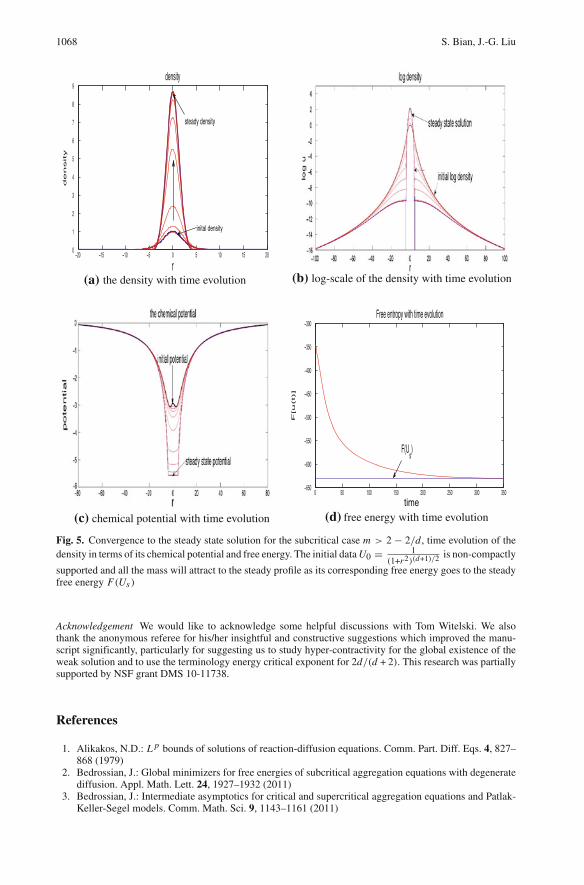
1068 S. Bian, J.-G. Liu
(a) the density with time evolution (b) log-scale of the density with time evolution
(c) chemical potential with time evolution (d) free energy with time evolution
Fig. 5. Convergence to the steady state solution for the subcritical case m > 2 − 2/d, time evolution of thedensity in terms of its chemical potential and free energy. The initial data U0 = 1
(1+r2)(d+1)/2 is non-compactly
supported and all the mass will attract to the steady profile as its corresponding free energy goes to the steadyfree energy F(Us )
Acknowledgement We would like to acknowledge some helpful discussions with Tom Witelski. We alsothank the anonymous referee for his/her insightful and constructive suggestions which improved the manu-script significantly, particularly for suggesting us to study hyper-contractivity for the global existence of theweak solution and to use the terminology energy critical exponent for 2d/(d + 2). This research was partiallysupported by NSF grant DMS 10-11738.
References
1. Alikakos, N.D.: L p bounds of solutions of reaction-diffusion equations. Comm. Part. Diff. Eqs. 4, 827–868 (1979)
2. Bedrossian, J.: Global minimizers for free energies of subcritical aggregation equations with degeneratediffusion. Appl. Math. Lett. 24, 1927–1932 (2011)
3. Bedrossian, J.: Intermediate asymptotics for critical and supercritical aggregation equations and Patlak-Keller-Segel models. Comm. Math. Sci. 9, 1143–1161 (2011)

Dynamic and Steady States for Multi-Dimensional Keller-Segel Model 1069
4. Bedrossian, J., Rodríguez, N., Bertozzi, A.L.: Local and global well-posedness for aggregation equationsand Patlak-Keller-Segel models with degenerate diffusion. Nonlinearity. 24, 1683–1714 (2011)
5. Berestycki, H.: Le nombre de solutions de certains problemes semi-lineaires elliptique. J. Funct.Anal. 40, 1–29 (1981)
6. Blanchet, A., Bonforte, M., Dolbeault, J., Grillo, G., Vázquez, J.L.: Asymptotics of the Fast DiffusionEquation via Entropy Estimates. Arch. Rati. Mech. Anal. 91, 347–385 (2009)
7. Blanchet, A., Carrillo, J.A., Laurencot, P.: Critical mass for a Patlak-Keller-Segel model with degeneratediffusion in higher dimensions. Calc. Var. 35, 133–168 (2009)
8. Blanchet, A., Carrillo, J.A., Masmoudi, N.: Infinite time aggregation for the critical Patlak-Keller- Segelmodel in R
2. Comm. Pure Appl. Math. 61, 1449–1481 (2008)9. Blanchet, A., Dolbeault, J., Perthame, B.: Two- dimensional Keller-Segel model: optimal critical mass
and qualitative properties of the solutions. Eletron. J. Diff. Eq. 44, 1–33 (2006)10. Brenner, M.P., Constantin, P., Kadanoff, L.P., Schenkel, A., Venkataramani, S.C.: Diffusion, attraction
and collapse. Nonlinearity 12, 1071–1098 (1999)11. Brenner, M.P., Witelski, T.P.: On spherically symmetric gravitational collapse. J. Stat. Phys. 93, 863–
900 (1998)12. Caffarelli, L.A., Gidas, B., Spruck, J.: Asymptotic symmetry and local behavior of semilinear elliptic
equations with critical Sobolev growth. Comm. Pure Appl. Math. 42, 271–297 (1989)13. Calvez, V., Corrias, L., Ebde, M.A.: Blow-up, concentration phenomenon and global existence for the
Keller-Segel model in high dimension. Comm. Part. Diff. Eq. 37(4), 561–584 (2012)14. Carlen, E.A., Carrillo, J.A., Loss, M.: Hardy-Littlewood-Sobolev inequalities via fast diffusion flows.
Proc. Nat. Acad. USA 107, 19696–19701 (2010)15. Chandrasekhar, S.: An Introduction to the Study of Stellar Structure. New York: Dover, 196716. Chen, W.X., Li, C.M.: Classification of solutions of some nonlinear elliptic equations. Duke Math.
J. 63, 333–364 (1991)17. Chen, L., Liu, J.-G., Wang, J.: Multi-dimensional degenerate Keller-Segel system with critical diffusion
exponent 2n/(n + 2). SIAM J. Math. Anal. 44, 1077–1102 (2012)18. Dancer, E.N., Guo, Z., Wei, J.C.: Non-radial solutions of Lane-Emden equation in R
n . Indiana UnivMath J. to appear
19. Degond, P., Liu, J.-G., Ringhofer, C.: Large-scale dynamics of Mean-Field Games driven by local Nashequilibria. J. Nonlinear Sci. to appear
20. Gidas, B., Ni, W.M., Nirenberg, L.: Symmetry and related properties via the maximum principle. Com-mun. Math. Phys. 68, 209–243 (1979)
21. Gidas, B., Ni, W.M., Nirenberg, L.: ”Symmetry of positive solutions of nonlinear elliptic equations inRn”. In: Mathematical Analysis and Applications, Part A, ed. L. Nachbin, Adv. Math. Suppl. Stud. 7,New York: Academic Press, 1981, pp. 369–402
22. Gidas, B., Spruck, J.: Global and local behavior of positive solutions of nonlinear elliptic equations.Comm. Pure Appl. Math. 34, 525–598 (1981)
23. Gui, C., Ni, W.M., Wang, X.F.: On the stability and instability of positive steady states of a semilinearheat equation in Rn . Comm. Pure Appl. Math. 45, 1153–1181 (1992)
24. Guo, Z.M.: On the symmetry of positive solutions of the Lane-Emden equation with super-critical expo-nent. Adv. Diff. Eqs. 7, 641–666 (2002)
25. Herrero, M., Medina, E., Velázquez, J.L.: Finite-time aggregation into a single point in a reaction-diffusionsystem. Nonlinearity 10, 1739–1754 (1997)
26. Herrero, M., Medina, E., Velázquez, J.L.: Self-similar blow-up for a reaction-diffusion system. J. Comp.Appl. Math. 97, 99–119 (1998)
27. Herrero, M.A., Pierre, M.: The Cauchy problem for ut = �um when 0 < m < 1. Trans. AMS. 291, 145–158 (1985)
28. Jäger, W., Luckhaus, S.: On explosions of solutions to a system of partial differential equations modelingchemotaxis. Trans. Amer. Math. Soc. 239(2), 819–821 (1992)
29. Joseph, D.D., Lundgren, T.S.: Quasilinear Dirichlet problems driven by positive sources. Arch. Rat. Mech.Anal. 49, 241–269 (1973)
30. Keller, E.F., Segel, L.A.: Initiation of slime mold aggregation viewed as an instability.J. Theor. Biol. 26, 399–415 (1970)
31. Kim, I., Yao, Y.: The Patlak-Keller-Segel model and its variations: properties of solutions via maximumprinciple. SIAM J. Math. Anal. 44, 568–602 (2012)
32. Laugesen, R.S., Pugh, M.C.: Properties of steady states for thin film equations. Eur. J. Appl. Math. 11, 293–351 (2000)
33. Lieb, E.H.: Sharp constants in the Hardy-Littlewood-Sobolev and related inequalities.Ann. Math. 118(2), 349–374 (1983)

1070 S. Bian, J.-G. Liu
34. Lieb, E.H., Loss, M.: Analysis, Graduate Studies in Mathematics. V. 14, Providence, RI: Amer. Math.Soc., 2nd edition, 2001
35. Lions, P.L.: On the existence of positive solutions of semilinear elliptic equations. SIAM Rev. 24(4), 441–467 (1982)
36. Lions, P.L.: The concentration-compactness principle in calculus of variations. The locally compact case,part 1. Ann. Inst. Henri. Poincare. 1, 109–145 (1984)
37. Perthame, B: Transport Equations in Biology. Basel-Boston-Berlin: Birkhaeuser Verlag, 200738. Pohozaev, S.I.: Eigenfunctions of the equation �u + λ f (u) = 0. Sov. Math. 5, 1408–1411 (1965)39. Ströhmer, G.: Stationary states and moving planes. Banach Center Publ. 81, 501–513 (2008)40. Sugiyama, Y.: Global existence in sub-critical cases and finite time blow-up in super-critical cases to
degenerate keller-segel systems. Diff. Int. Eqs. 19, 841–876 (2006)41. Sugiyama, Y., Kunii, H.: Global existence and decay properties for a degenerate keller-segel model with
a power factor in drift term. J. Diff. Eqs. 227, 333–364 (2006)42. Sugiyama, Y., Yahagi, Y.: Extinction, decay and blow-up for Keller-Segel system of fast diffusion type.
J. Diff. Eqs. 250, 3047–3087 (2011)43. Vázquez, J.L.: Smoothing and Decay Estimates for Nonlinear Diffusion Equations. Equations of Porous
Medium Type. Oxford Lecture Ser. Math. Appl., Vol. 33, Oxford: Oxford Univ. Press, 200644. Vázquez, J.L.: The Porous Medium Equation: Mathematical Theory. Oxford: Oxford University Press,
200745. Weinstein, M.I.: Nonlinear Schrödinger equations and sharp interpolation estimates. Commun. Math.
Phys. 87, 567–576 (1983)46. Witelski, T.P.: Computing finite-time singularities in interfacial flows. In: Modern methods in scientific
computing and applications, NATO Sci. Ser. II Math. Phys. Chem. 75, Dordrecht: Kluwer Acad. Publ.,2002, pp. 451–487
47. Witelski, T.P., Bernoff, A.J., Bertozzi, A.L.: Blowup and dissipation in critical-case unstable thin filmequaion. Eur. J. Appl. Math. 15, 223–256 (2004)
48. Yao, Y., Bertozzi, A.L.: Blow-up dynamics for the aggregation equation with degenerate diffusion. Phy-sica D (2013), doi:10.1016/j.physd.2013.01.009
49. Zou, H.H.: Symmetry of positive solutions of �u + u p = 0 in Rn . J. Diff. Eqns. 120, 46–88 (1995)
Communicated by P. Constantin
![Two-dimensional modeling of steady state heat …Two-dimensional modeling of steady state heat transfer in solids with use of spreadsheet (MS EXCEL)] Spring 2011 1-2 BRIEF SUMMARY](https://img.pdfslide.us/doc/110x75/5aa25be67f8b9a436d8cdb16/two-dimensional-modeling-of-steady-state-heat-two-dimensional-modeling-of-steady.jpg)