Embed Size (px)
Citation preview

Master's Degree Thesis
ISRN: BTH-AMT-EX--2005/D-09--SE
Supervisor: Claes Hedberg, Docent, Ph.D. Mech. Eng.
Department of Mechanical Engineering Blekinge Institute of Technology
Karlskrona, Sweden
2005
Vidya Sagar Avadutala
Dynamic Analysis of cracks in Composite Materials

Dynamic Analysis of cracks in Composite Materials
Vidya Sagar Avadutala
Department of Mechanical Engineering Blekinge Institute of Technology SE-371 79 Karlskrona, Sweden
2005 Thesis submitted for completion of Master of Science in Mechanical Engineering with emphasis on Structural Mechanics at the Department of Mechanical Engineering, Blekinge Institute of Technology, Karlskrona, Sweden. Abstract:
Dynamic analysis of damages in materials is a difficult task and it is currently not known what important different possible mechanisms carry in the materials. It is to a large extent due to the difficulty of measuring the dynamic behavior of cracks, debonds and delaminations inside the material, there should exists a need to simulate the action of different mechanisms in order to understand the basic physics and possibly identifying the signatures of measured vibration and acoustic signals. In this work we study vibrational responses from a specimen which has different types of non-linearities like fractures in it at different locations and understand various factors concerned with fracture location, fracture behavior and so on.
Keywords:
Dynamic analysis, Cracks, Debonds, Delaminations, Acoustic signals, Stress intensity factors.
Acknowledgements This work was carried out at the Department of Mechanical Engineering, Blekinge Institute of Technology, Karlskrona, Sweden, Under the Supervision of Dr. Claes Hedberg.
I would like to express my sincere gratitude to Dr.Claes Hedberg for his guidance and support throughout my work. With out him I will never be able to complete my work with this ease.
I would like to thank Mr. Pierre Marty at CSM Materialteknik for his help and explanations.
Thanking you God for giving me the chance to pursue my academic goals and a wonderful, complete life full of amazing people.
And last but not least my parents, Murty, Mala and my sister Sravanthi gave me enormous strength, confidence and ability to work in good, healthy environment.
Karlskrona, February 2005 Vidya Sagar Avadutala
2
Table of contents
1. Notation 6 2. Introduction 8
2.1. Thesis background 8 2.2. Fracture and Damage Mechanics 8 2.3. Damages in Heterogeneous Materials 9 2.4. Geometric nonlinearities 10 2.5. Material nonlinearities 10
2.5.1. Cracks 11 2.5.2. Debonds 12 2.5.3. Delaminations 12
2.6. Motivation to the Approach 13 3. Theory and concepts 14
3.1. Linear Elastic Fracture Mechanics 14 3.2. Frequency, wavelength and Time period 14 3.3. Mechanical waves 15
3.3.1. Reflection at interface 16 3.4. Variable Amplitude Loading 17 3.5. Integration Time step or Step size 18 3.6. Nonlinear Dynamics and Damage 19 3.7. Plasticity 19
4. Dynamic Analysis 21
4.1. Homogeneous material 21 4.1.1. Analytical Data and Calculations 21 4.1.2. Modeling 21 4.1.3. Frequency Analysis 23 4.1.4. Dynamic Analysis 25 4.1.5. Results 32
4.2. Homogeneous material with crack 36 4.2.1. Analytical Data and Calculations 36 4.2.2. Modeling 36 4.2.3. Frequency Analysis 38 4.2.4. Dynamic Analysis 39 4.2.5. Results 43
3
4.2.5.1.Homogenous material with fixed crack 46 4.3. Heterogeneous material 51
4.3.1. Analytical Data and Calculations 51 4.3.2. Modeling 51 4.3.3. Frequency Analysis 53 4.3.4. Dynamic Analysis 54 4.3.5. Results 57
4.4. Heterogeneous material with crack 60 4.4.1. Modeling 60 4.4.2. Frequency Analysis 61 4.4.3. Dynamic Analysis 63 4.4.4. Results 64
5. Conclusions 70
6. Further approach to work 71
7. References 72
4

Appendices 73
A. Code for dynamic analysis of homogeneous material. 73 B. Code for dynamic analysis of homogeneous material with crack. 75 C. Code for dynamic analysis of heterogeneous material. 77 D. Code for dynamic analysis of heterogeneous material with crack. 79 E. Code for dynamic analysis of composite laminate material with
crack. 81 F. Table of pictures 83
5
1 Notation a Crack length
pc Velocity of Pressure wave
ppc Velocity of Pressure wave
sc Velocity of Shear wave
E Young’s modulus
F Frequency
fxf Flexural frequency
tf Thickness frequency
G Shear modulus
1K Stress Intensity factor
R Reflection coefficient
yr Plastic zone radius
T Depth of crack from surface
fxT Flexural time period
t Time period
Z Specific acoustic impedance
v Velocity of shear wave
λ Wavelength
υ Poisson’s ratio
ρ Density
θ Angle of Plastic zone from crack tip
YSσ Ultimate shear stress
6
Indices fx Flexural
YS Yield strength
p Pressure wave
s Shear wave Abbreviations ANSYS Analysis Software
AISI American Iron & Steel Institute
DOF’S Degrees of freedom
ITS Integration time step
LEFM Linear Elastic Fracture Mechanics
NDT Non Destructive Testing
7
2 Introduction 2.1 Thesis background In homogeneous material systems, damage almost always involves cracks. From dynamics and fracture mechanics, it is well known that accelerated crack nucleation and micro-crack formation in components can occur due to various reasons, such as transient load swings, higher than expected intermittent loads, or defective component materials. Normal wear causes configuration changes that contribute to dynamic loading conditions that can cause micro-crack formation at material grain boundaries in stress concentrated regions (acute changes in material geometry) [1].
Structural systems may be composed of homogeneous or heterogeneous materials such as composites, plastics, ceramics, fabrics and metal-alloys. Heterogeneous structures have complicated dynamics of their own in addition to numerous types of damage and failure modes (crack growth, delaminations, fiber breakage, matrix cracking, component failures), which interact in complicated ways that vary tremendously for different initial states, levels of damage accumulation and loading history, making it very difficult to forecast their remaining useful life in operation. Though there have been abundant, relatively successful efforts to model and predict specific types of failure in complex material and structural systems, this work is directed towards the investigation of a more universal approach ‘time-domain’ technique can accommodate the diversity of failure modes exhibited by structures. This work is mainly concerned about time-domain plots for various types of damages in composite as well as homogeneous materials. 2.2 Fracture and Damage Mechanics Cracks and flaws occur in many structures and components, sometimes leading to disastrous results. The engineering field of fracture mechanics was established to develop a basic understanding of such crack propagation problems.
Fracture mechanics deals with the study of how a crack or flaw in a
8
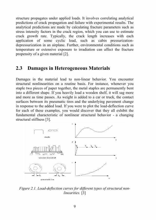
structure propagates under applied loads. It involves correlating analytical predictions of crack propagation and failure with experimental results. The analytical predictions are made by calculating fracture parameters such as stress intensity factors in the crack region, which you can use to estimate crack growth rate. Typically, the crack length increases with each application of some cyclic load, such as cabin pressurization-depressurization in an airplane. Further, environmental conditions such as temperature or extensive exposure to irradiation can affect the fracture propensity of a given material [2]. 2.3 Damages in Heterogeneous Materials Damages in the material lead to non-linear behavior. You encounter structural nonlinearities on a routine basis. For instance, whenever you staple two pieces of paper together, the metal staples are permanently bent into a different shape. If you heavily load a wooden shelf, it will sag more and more as time passes. As weight is added to a car or truck, the contact surfaces between its pneumatic tires and the underlying pavement change in response to the added load. If you were to plot the load-deflection curve for each of these examples, you would discover that they all exhibit the fundamental characteristic of nonlinear structural behavior - a changing structural stiffness [3].
Figure 2.1. Load-deflection curves for different types of structural non-linearities. [3]
9
Nonlinear structural behavior arises from a number of causes, which can be grouped into these principal categories:
• Geometric nonlinearities
• Material nonlinearities 2.4 Geometric nonlinearities If a structure experiences large deformations, its changing geometric configuration can cause the structure to respond nonlinearly. Geometric nonlinearity is characterized by "large" displacements and rotations [3]. 2.5 Material nonlinearities A number of material-related factors can cause your structure's stiffness to change during the course of an analysis. Nonlinear stress-strain relationships of plastic, multilinear elastic, and hyperelastic materials will cause a structure's stiffness to change at different load levels (and, typically, at different temperatures). Creep, viscoplasticity, and viscoelasticity will give rise to nonlinearities that can be time, rate, temperature, and stress-related. Swelling will induce strains that can be a function of temperature, time, neutron flux level (or some analogous quantity), and stress [3].
As mentioned above Viscoplasticity can occur because of fracture. This occurs at near crack tip field with certain radius of curvature. Plasticity region highly depend of type of material in which fracture situated and plane strain and plane stress conditions. Non-linearity due to crack is differ from non-linearity occur due to plasticity around the crack tip, which is detailed in later chapters. Some types of non-linear causing damages are explained below.
10
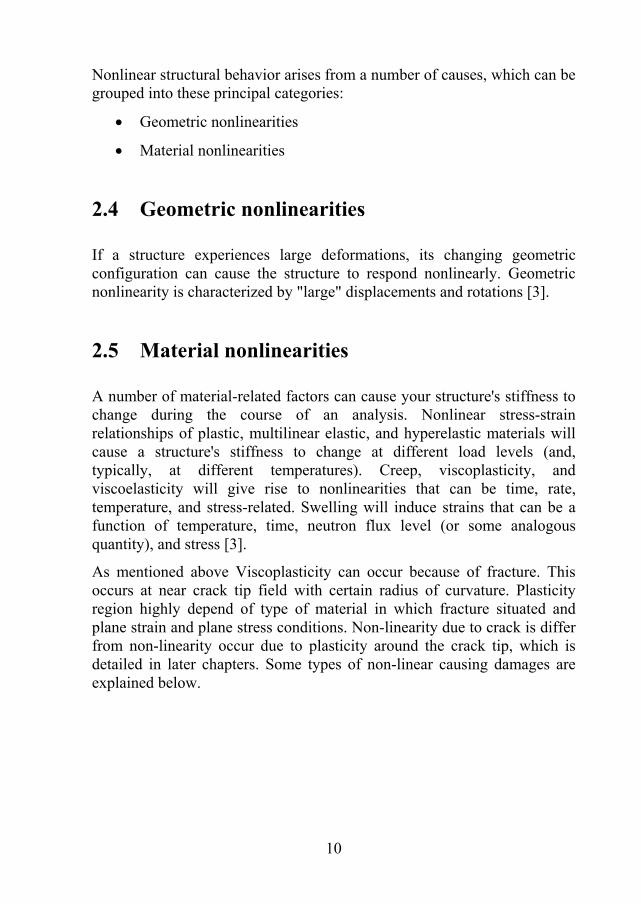
2.5.1 Cracks A crack is a type of fracture that separates a solid body into two, or more, pieces under the action of stress. There are three types of modes of failure [4].
Mode I: The forces are perpendicular to the crack (the crack is horizontal and the forces are vertical), pulling the crack open. This is referred to as the opening mode.
Mode II: The forces are parallel to the crack. One force is pushing the top half of the crack back and the other is pulling the bottom half of the crack forward, both along the same line. This creates a shear crack: the crack is sliding along itself. It is called in-plane shear because the forces are not causing the material to move out of its original plane.
Mode III: The forces are perpendicular to the crack (the crack is in front-back direction, the forces are pulling left and right). This causes the material to separate and slide along itself, moving out of its original plane (which is why it’s called out-of-plane shear).
Figure 2.2. Three loading modes.
11
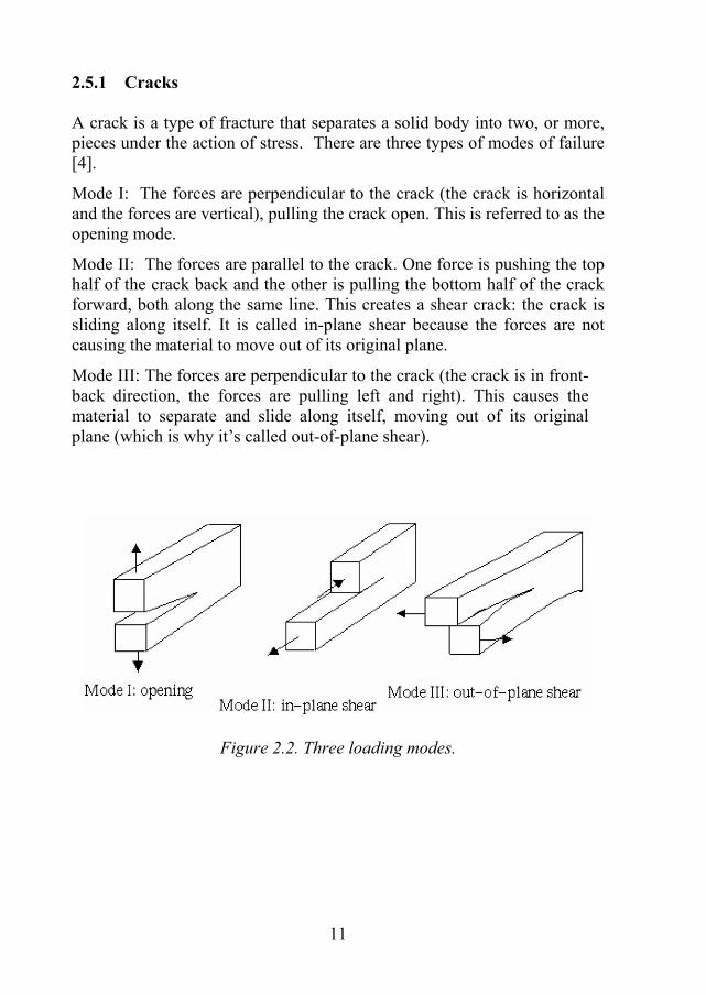
2.5.2 Debonds Debonds are type of fractures where the bonding between the material molecules are vulnerable to breakage. These occur in weak strength materials more often. These are due to mould defects during manufacturing. 2.5.3 Delaminations One of the most commonly observed failure modes in composite materials is delamination, a separation of the fiber reinforced layers that are stacked together to form laminates. The most common sources of delamination are the material and structural discontinuities shown in figure 2.3. Delaminations occur at stress free edges due to the mismatch in properties of the individual layers, at ply drops where thickness must be reduced, and at regions subjected to out-of-plane loading such as bending of curved beams.
Figure 2.3. Different types of Delaminations.
12

2.6 Motivation to the Approach Nonlinear dynamic analysis can be a very interesting tool to detect as well as to understand the damaged materials. Predicting the intensity of damage before the system failures is one of the major interests in modeling and as well as manufacturing. Dynamic analysis is particularly very in the field of detecting the damages in composites and homogeneous materials. Gaining the knowledge about dynamic analysis (time-domain technique) is very essential in every aspect of nonlinear damage detection in huge structures like bridges and even very small things like computer components. This work leads to inspiring questions regarding the damages.
13
3 Theory and concepts
3.1 Linear Elastic Fracture Mechanics The concepts of fracture mechanics that were derived prior to 1960 are applicable only to materials that obey Hooke’s law. Although corrections for small scale plasticity were proposed as early as 1948, these analyses are restricted to structures whose global behavior is linear elastic [2].
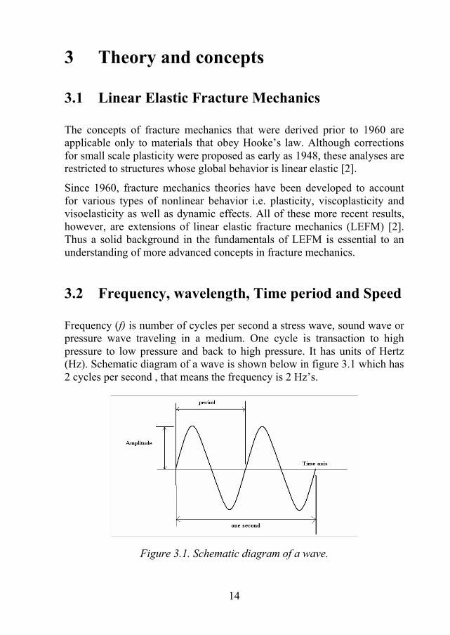
Since 1960, fracture mechanics theories have been developed to account for various types of nonlinear behavior i.e. plasticity, viscoplasticity and visoelasticity as well as dynamic effects. All of these more recent results, however, are extensions of linear elastic fracture mechanics (LEFM) [2]. Thus a solid background in the fundamentals of LEFM is essential to an understanding of more advanced concepts in fracture mechanics. 3.2 Frequency, wavelength, Time period and Speed Frequency (f) is number of cycles per second a stress wave, sound wave or pressure wave traveling in a medium. One cycle is transaction to high pressure to low pressure and back to high pressure. It has units of Hertz (Hz). Schematic diagram of a wave is shown below in figure 3.1 which has 2 cycles per second , that means the frequency is 2 Hz’s.
Figure 3.1. Schematic diagram of a wave.
14
Wave length is the distance between two consecutive crests of wave.
Wavelength (λ ) = speed of sound (speed of stress wave)/frequency of oscillation.
The period (t) of a function (displacement versus time, for instance) shows the interval (on time axes) between the points where a given dependence repeats its value. It is apparent that frequency is equal to the reciprocal of the period.
f = 1 / t. (3.1)
Speed ( v ) the velocity of propagation of a traveling wave: fv λ= . 3.3 Mechanical waves A mechanical wave is a disturbance which moves through some medium. Mechanical waves are one types of stress wave’s travel through solid materials. These have different velocities in different metals depending on the young’s modulus of that material and Poisson’s ratio. For inspecting the damages in materials there is a great need to inspect this stress waves properties and how this stress wave travels in that medium. An electro-mechanical transducer is used to generate this ultrasonic stress waves that propagates into the object being inspected. Reflection of the stress pulse occurs at boundaries separating materials with different densities and elastic properties. The reflected pulse or signal travels back to the transducer that also acts as a receiver. The received signal is displayed on an oscilloscope, and the round trip travel time of the pulse is measured electronically. By knowing the speed of the stress wave, the distance to the reflecting interface can be determined.
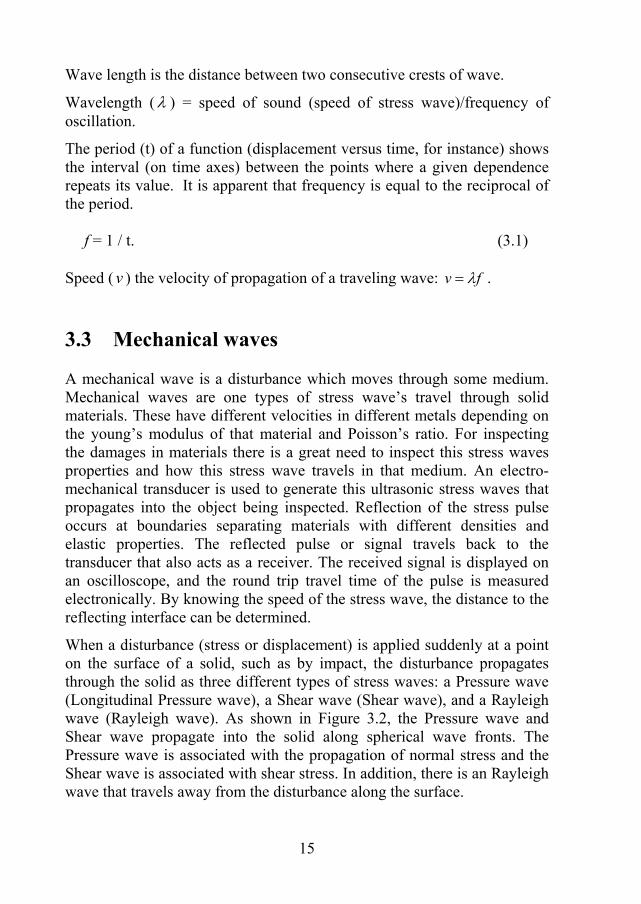
When a disturbance (stress or displacement) is applied suddenly at a point on the surface of a solid, such as by impact, the disturbance propagates through the solid as three different types of stress waves: a Pressure wave (Longitudinal Pressure wave), a Shear wave (Shear wave), and a Rayleigh wave (Rayleigh wave). As shown in Figure 3.2, the Pressure wave and Shear wave propagate into the solid along spherical wave fronts. The Pressure wave is associated with the propagation of normal stress and the Shear wave is associated with shear stress. In addition, there is an Rayleigh wave that travels away from the disturbance along the surface.
15
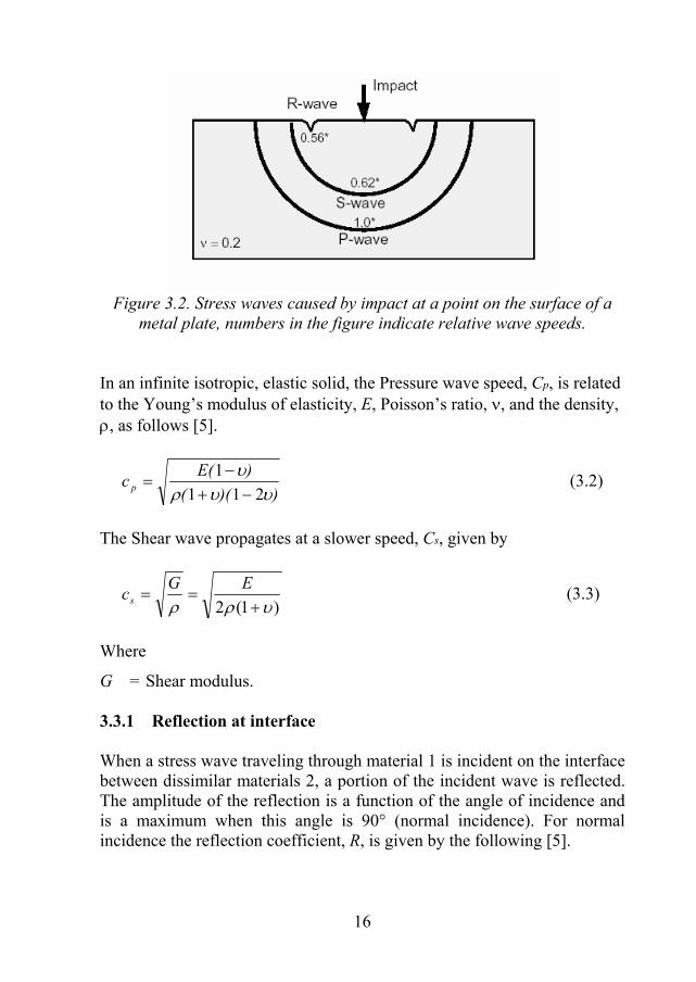
Figure 3.2. Stress waves caused by impact at a point on the surface of a
metal plate, numbers in the figure indicate relative wave speeds. In an infinite isotropic, elastic solid, the Pressure wave speed, Cp, is related to the Young’s modulus of elasticity, E, Poisson’s ratio, ν, and the density, ρ, as follows [5].
))(()E(c p υυρ
υ211
1−+
−= (3.2)
The Shear wave propagates at a slower speed, Cs, given by
)1(2 υρρ +==
EGcs (3.3)
Where
G = Shear modulus. 3.3.1 Reflection at interface When a stress wave traveling through material 1 is incident on the interface between dissimilar materials 2, a portion of the incident wave is reflected. The amplitude of the reflection is a function of the angle of incidence and is a maximum when this angle is 90° (normal incidence). For normal incidence the reflection coefficient, R, is given by the following [5].
16
12
12
ZZZZR
+−
= (3.4)
Where
1Z = specific acoustic impedance of material 1.
2Z = specific acoustic impedance of material 2. The specific acoustic impedance is the product of the wave speed and density of the material. The following are approximate Z-values for some materials [6].
Material
Specific acoustic impedance, kg/(m2 s)
Air 0.4 Water 0.5 x 10⁶ Soil 0.3 to 4 x 10⁶
Concrete 7 to 10 x 106 Steel 47 x 106
Table 3.1 Impedances of some materials.
Thus, when a stress wave traveling through metal encounters an interface with air, there is almost total reflection at the interface. This is why Non destructive (NDT) methods based on stress wave propagation have proven to be successful for locating defects within solids. 3.4 Variable Amplitude Loading When dealing with dynamic analysis there is a need to introduce a time factor. Any form of dynamic excitation can be composed from series of short impulses (see Figure 3.3). By Calculating a short impulse and increase that with a small step size will produce a dynamic excitation. This step size which is also called as Integration time step (ITS) is very important during dealing with nonlinearities such as plasticity .It is also important to notice that we can simulate this impulse load by applying initial velocity conditions in Newmark's integration [3]. In this thesis work
17
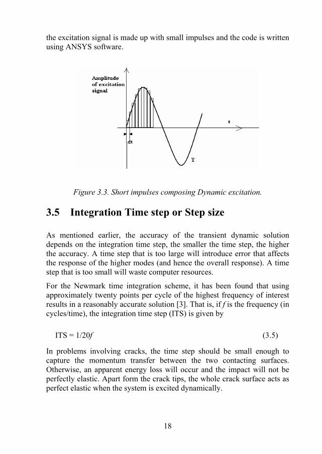
the excitation signal is made up with small impulses and the code is written using ANSYS software.
Figure 3.3. Short impulses composing Dynamic excitation. 3.5 Integration Time step or Step size As mentioned earlier, the accuracy of the transient dynamic solution depends on the integration time step, the smaller the time step, the higher the accuracy. A time step that is too large will introduce error that affects the response of the higher modes (and hence the overall response). A time step that is too small will waste computer resources.
For the Newmark time integration scheme, it has been found that using approximately twenty points per cycle of the highest frequency of interest results in a reasonably accurate solution [3]. That is, if f is the frequency (in cycles/time), the integration time step (ITS) is given by
ITS = 1/20f (3.5)
In problems involving cracks, the time step should be small enough to capture the momentum transfer between the two contacting surfaces. Otherwise, an apparent energy loss will occur and the impact will not be perfectly elastic. Apart form the crack tips, the whole crack surface acts as perfect elastic when the system is excited dynamically.
18
3.6 Nonlinear Dynamics and Damage Damages can occur in many different materials due to progressive and prolonged loading and environmental effects such as the excessive temperatures, temperature differences. There is a great need to find the damaged parts in the material before it is going to fail. There are so many methods proposed for detecting and analyzing the damages mainly internal damages, but none of them match up to the dynamic analysis efficiency. Behavior of the stress near internal damages needs to be analyzed for further progress in the identification of damages. Nonlinear dynamics is concerned with the softening, stiffening, opening and closing the fracture, sliding and impacts caused by fasteners etc. observing the time dependent factors near the internal damages is the main concern for the nonlinear dynamics see figure 3.4. 3.7 Plasticity Most common engineering materials exhibit a linear stress-strain relationship up to a stress level known as the proportional limit. Beyond this limit, the stress-strain relationship will become nonlinear, but will not necessarily become inelastic. Plastic behavior, characterized by non- recoverable strain, begins when stresses exceed the material's yield point.
Plasticity is a non-conservative, path-dependent phenomenon. In other words, the sequence in which loads are applied and in which plastic responses occur affects the final solution results [2]. If you anticipate plastic response in your analysis, you should apply loads as a series of small incremental load steps or time steps, so that your model will follow the load-response path as closely as possible. Plastic deformation will occur in regions near the crack tip where the stresses exceed the yield stress. This plastic deformation results in relaxation of stresses in the plastic zone. Plastic zone shapes for plane stress condition for mode 1 type of loading is shown in below [2].
19
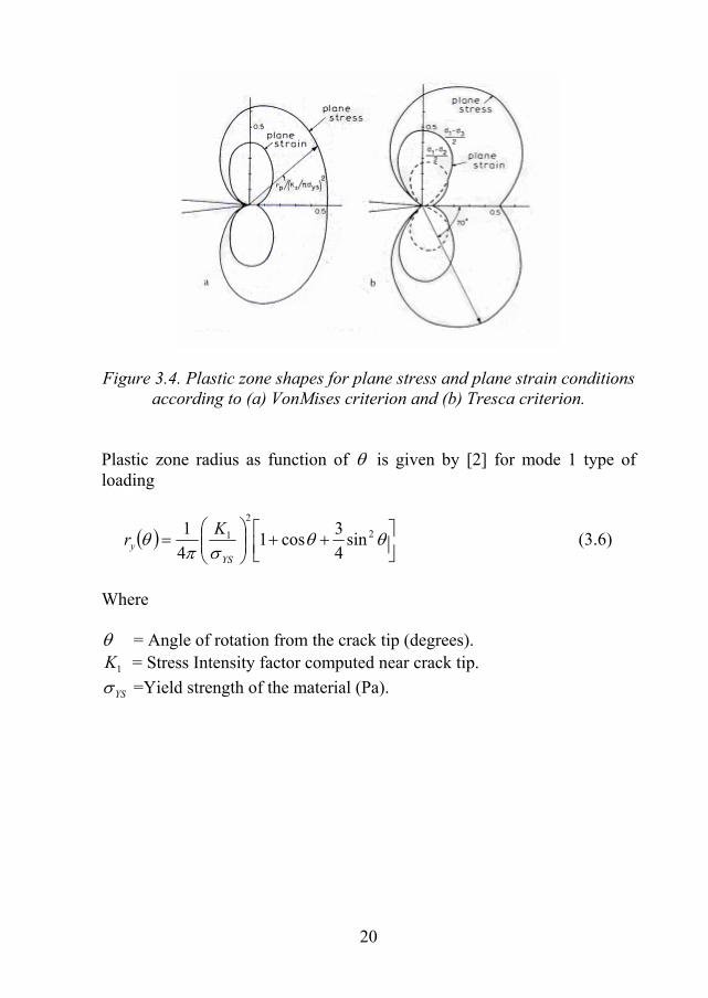
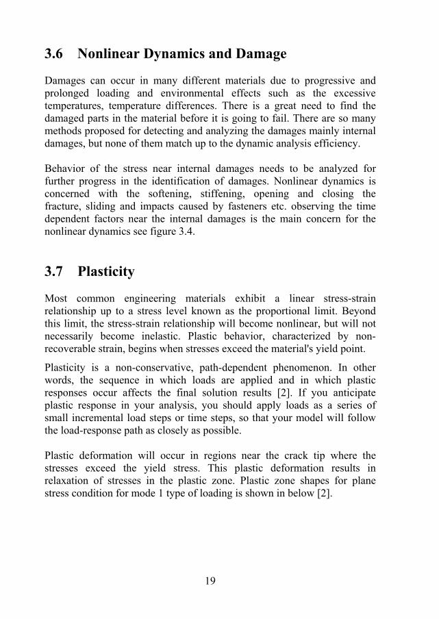
Figure 3.4. Plastic zone shapes for plane stress and plane strain conditions according to (a) VonMises criterion and (b) Tresca criterion.
Plastic zone radius as function of θ is given by [2] for mode 1 type of loading
( ) ⎥⎦⎤
⎢⎣⎡ ++⎟⎟
⎠
⎞⎜⎜⎝
⎛= θθ
σπθ 2
2
1 sin43cos1
41
YSy
Kr (3.6)
Where θ = Angle of rotation from the crack tip (degrees).
1K = Stress Intensity factor computed near crack tip.
YSσ =Yield strength of the material (Pa).
20
4 Dynamic Analysis 4.1 Homogeneous material 4.1.1 Analytical Data and Calculations Homogeneous material is assumed as Aluminum Alloy which is a non ferrous metal with the following material properties.
Density of Aluminium (ρ) = 2700 Kg/m3
Poisson’s ratio of Aluminium (υ ) = 0.3
Young’s modulus of Aluminium (E) = 7x10¹⁰ pa
Velocity of sound in Aluminium ( v ) is calculated form the equation (3.2) as
v = ))((
)E(c p υυρυ
2111
−+−
= = )3.021)(3.01(2700
)3.01(107 10
xx
−+− = 5907.64 m/s
In the early research leading to the development of the dynamic analysis, it was assumed that the wave speed across the thickness of the plate was the same as the Pressure wave speed in a large solid with small error [7], as given by the equation (3.2). 4.1.2 Modeling Aluminium is taken as homogeneous material and the modeling is done. Dimensions of the metal block are 1 x 0.5 m as seen in the Figure 4.1. A 2-D model is modeled and meshed with approximately 16 elements across the width of the metal block. To see the wave effects in the model when the force is applied, approximately 20 elements per wavelength is required, but here less than 20 elements are meshed across the width because to diminish the computer resources. 3-D model for dynamic analysis takes lot of computer resources so only 2-D model is done.
21
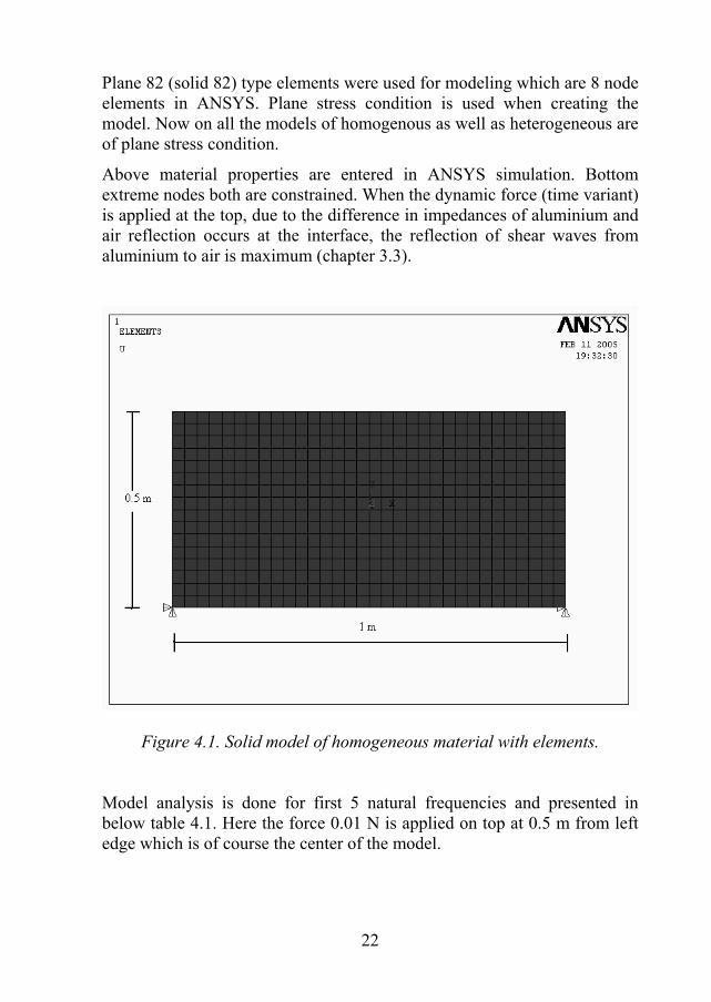
Plane 82 (solid 82) type elements were used for modeling which are 8 node elements in ANSYS. Plane stress condition is used when creating the model. Now on all the models of homogenous as well as heterogeneous are of plane stress condition.
Above material properties are entered in ANSYS simulation. Bottom extreme nodes both are constrained. When the dynamic force (time variant) is applied at the top, due to the difference in impedances of aluminium and air reflection occurs at the interface, the reflection of shear waves from aluminium to air is maximum (chapter 3.3).
Figure 4.1. Solid model of homogeneous material with elements.
Model analysis is done for first 5 natural frequencies and presented in below table 4.1. Here the force 0.01 N is applied on top at 0.5 m from left edge which is of course the center of the model.
22
Modes Modal frequencies (Hz) 1 629.26 2 634.63 3 845.15 4 1887.0 5 2649.0
Table 4.1.Modal frequencies for homogeneous model.
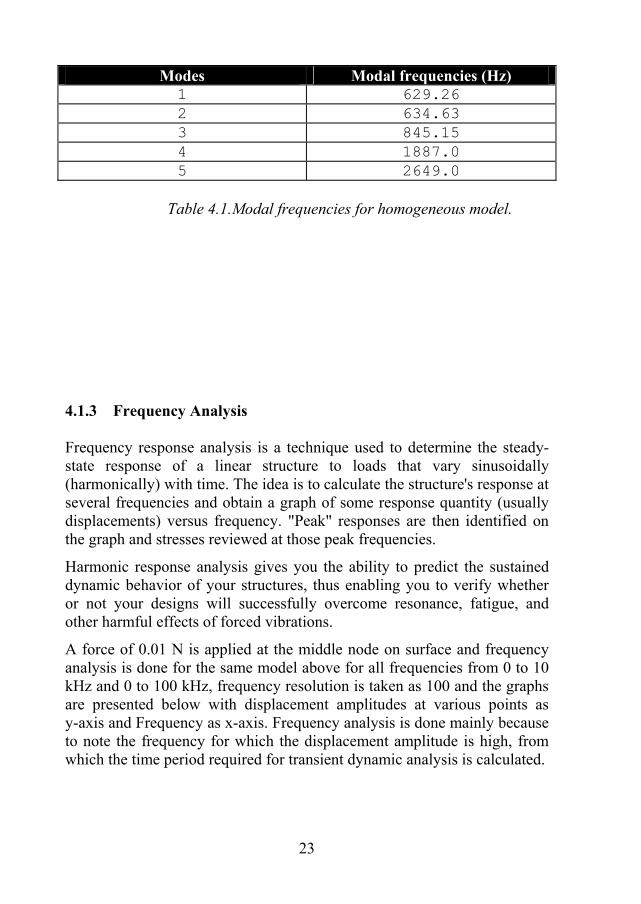
4.1.3 Frequency Analysis Frequency response analysis is a technique used to determine the steady-state response of a linear structure to loads that vary sinusoidally (harmonically) with time. The idea is to calculate the structure's response at several frequencies and obtain a graph of some response quantity (usually displacements) versus frequency. "Peak" responses are then identified on the graph and stresses reviewed at those peak frequencies.
Harmonic response analysis gives you the ability to predict the sustained dynamic behavior of your structures, thus enabling you to verify whether or not your designs will successfully overcome resonance, fatigue, and other harmful effects of forced vibrations.
A force of 0.01 N is applied at the middle node on surface and frequency analysis is done for the same model above for all frequencies from 0 to 10 kHz and 0 to 100 kHz, frequency resolution is taken as 100 and the graphs are presented below with displacement amplitudes at various points as y-axis and Frequency as x-axis. Frequency analysis is done mainly because to note the frequency for which the displacement amplitude is high, from which the time period required for transient dynamic analysis is calculated.
23
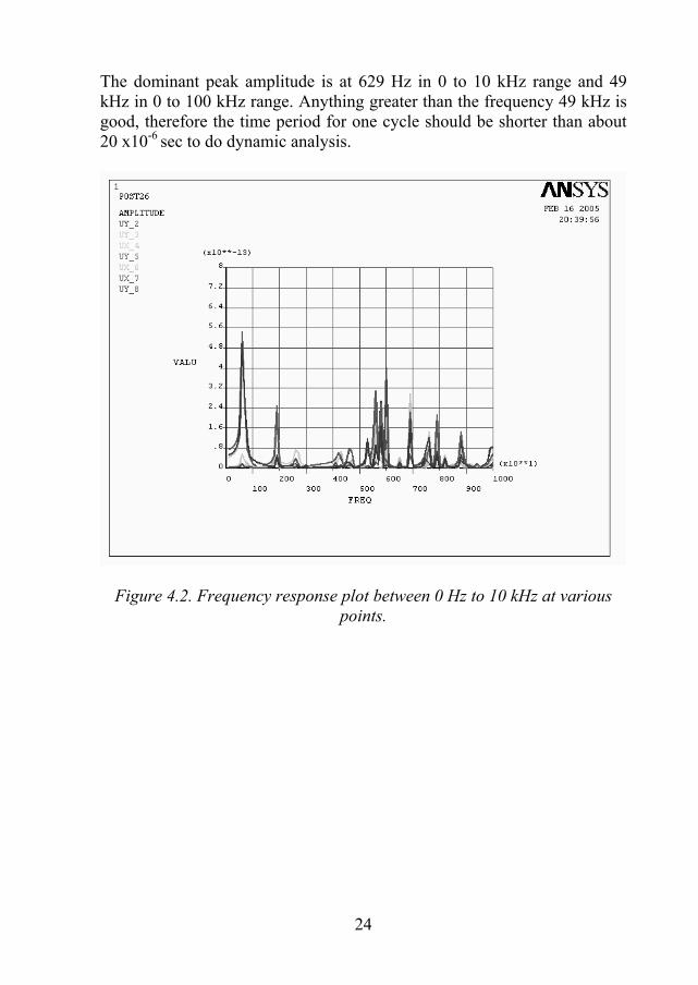
The dominant peak amplitude is at 629 Hz in 0 to 10 kHz range and 49 kHz in 0 to 100 kHz range. Anything greater than the frequency 49 kHz is good, therefore the time period for one cycle should be shorter than about 20 x10-6 sec to do dynamic analysis.
Figure 4.2. Frequency response plot between 0 Hz to 10 kHz at various points.
24
Figure 4.3. Frequency response plot between 0 Hz to 100 kHz at various points.
4.1.4 Dynamic Analysis Transient dynamic analysis (sometimes called time-history analysis) is a technique used to determine the dynamic response of a structure under the action of any general time-dependent loads. This analysis can be used to determine the time-varying displacements, strains, stresses, and forces in a structure as it responds to any combination of static, transient, and harmonic loads. The time scale of the loading is such that the inertia or damping effects are considered to be important.
As mentioned in chapter 3.4, the input (excitation) is a time variant force. Here the time variant force is a half sine curve with time as x-axis and force as y-axis, as mentioned in previous session the impact time is 1x10⁻⁵ sec, since one full period of sine wave is 2x10⁻⁵ sec (T = 1/f ).A MatLab graph of excitation is plotted and presented below.
25
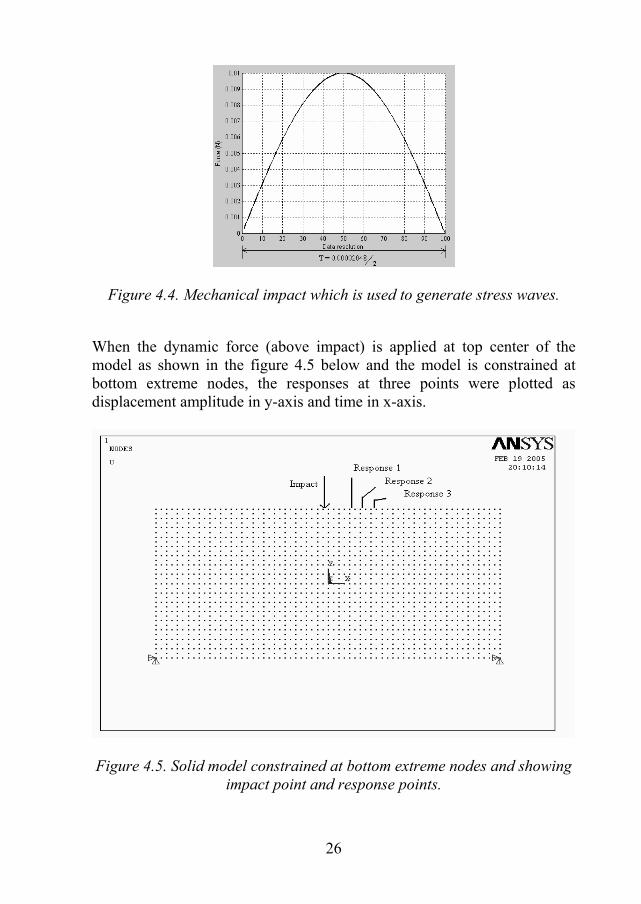
Figure 4.4. Mechanical impact which is used to generate stress waves.
When the dynamic force (above impact) is applied at top center of the model as shown in the figure 4.5 below and the model is constrained at bottom extreme nodes, the responses at three points were plotted as displacement amplitude in y-axis and time in x-axis.
Figure 4.5. Solid model constrained at bottom extreme nodes and showing
impact point and response points.
26
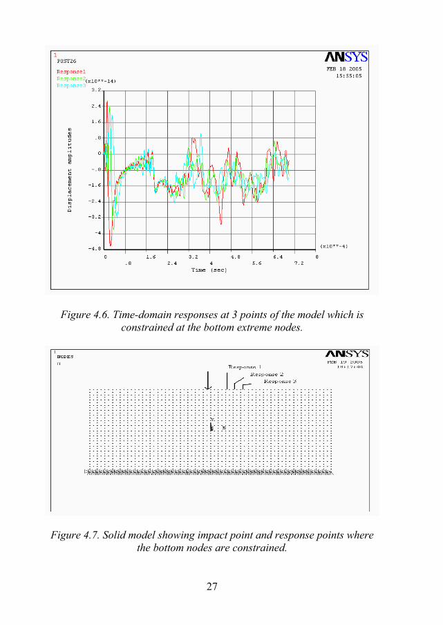
Figure 4.6. Time-domain responses at 3 points of the model which is constrained at the bottom extreme nodes.
Figure 4.7. Solid model showing impact point and response points where the bottom nodes are constrained.
27
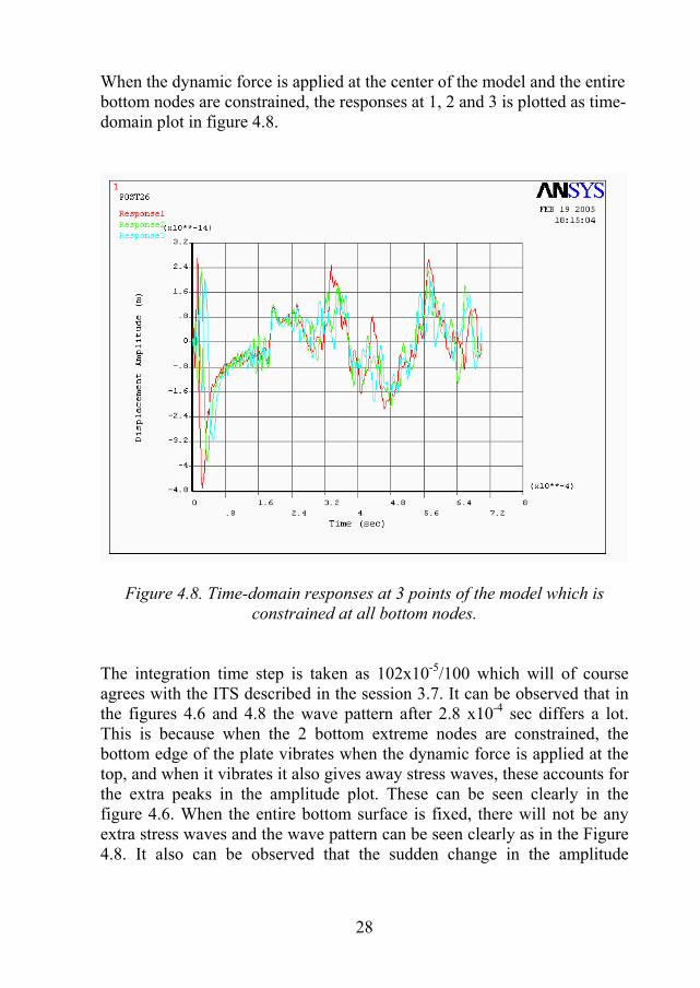
When the dynamic force is applied at the center of the model and the entire bottom nodes are constrained, the responses at 1, 2 and 3 is plotted as time-domain plot in figure 4.8.
Figure 4.8. Time-domain responses at 3 points of the model which is constrained at all bottom nodes.
The integration time step is taken as 102x10-5/100 which will of course agrees with the ITS described in the session 3.7. It can be observed that in the figures 4.6 and 4.8 the wave pattern after 2.8 x10⁻⁴ sec differs a lot. This is because when the 2 bottom extreme nodes are constrained, the bottom edge of the plate vibrates when the dynamic force is applied at the top, and when it vibrates it also gives away stress waves, these accounts for the extra peaks in the amplitude plot. These can be seen clearly in the figure 4.6. When the entire bottom surface is fixed, there will not be any extra stress waves and the wave pattern can be seen clearly as in the Figure 4.8. It also can be observed that the sudden change in the amplitude
28
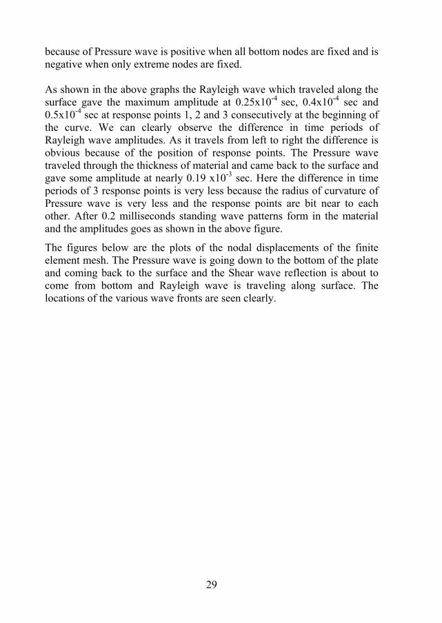
because of Pressure wave is positive when all bottom nodes are fixed and is negative when only extreme nodes are fixed. As shown in the above graphs the Rayleigh wave which traveled along the surface gave the maximum amplitude at 0.25x10⁻⁴ sec, 0.4x10⁻⁴ sec and 0.5x10⁻⁴ sec at response points 1, 2 and 3 consecutively at the beginning of the curve. We can clearly observe the difference in time periods of Rayleigh wave amplitudes. As it travels from left to right the difference is obvious because of the position of response points. The Pressure wave traveled through the thickness of material and came back to the surface and gave some amplitude at nearly 0.19 x10⁻³ sec. Here the difference in time periods of 3 response points is very less because the radius of curvature of Pressure wave is very less and the response points are bit near to each other. After 0.2 milliseconds standing wave patterns form in the material and the amplitudes goes as shown in the above figure.
The figures below are the plots of the nodal displacements of the finite element mesh. The Pressure wave is going down to the bottom of the plate and coming back to the surface and the Shear wave reflection is about to come from bottom and Rayleigh wave is traveling along surface. The locations of the various wave fronts are seen clearly.
29
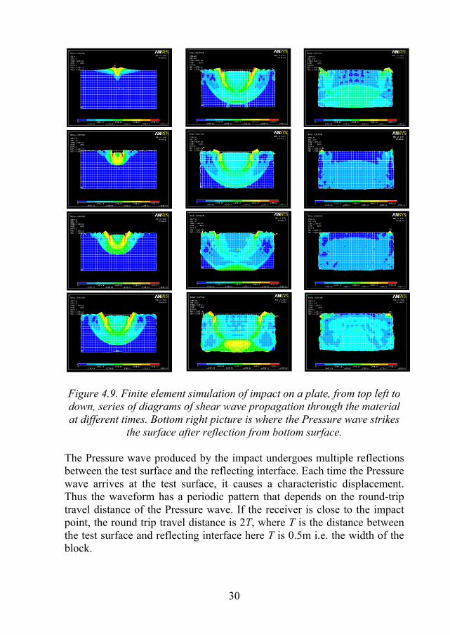
Figure 4.9. Finite element simulation of impact on a plate, from top left to down, series of diagrams of shear wave propagation through the material at different times. Bottom right picture is where the Pressure wave strikes
the surface after reflection from bottom surface. The Pressure wave produced by the impact undergoes multiple reflections between the test surface and the reflecting interface. Each time the Pressure wave arrives at the test surface, it causes a characteristic displacement. Thus the waveform has a periodic pattern that depends on the round-trip travel distance of the Pressure wave. If the receiver is close to the impact point, the round trip travel distance is 2T, where T is the distance between the test surface and reflecting interface here T is 0.5m i.e. the width of the block.
30
The time interval between successive arrivals of the multiply reflected Pressure wave is the travel distance divided by the wave speed. The frequency, f, of the Pressure wave arrival is the inverse the time interval and is given by the approximate relationship
Tc
f pp
2= (4.1)
Tc
tpp
21 =⇒
Where
ppc =0.96x [8] (4.2) pc
pc = Pressure wave speed through the thickness of the block.
T = Thickness of the block.
t = Time taken for Pressure wave to come to top after reflecting from the interface.
This frequency is also known as the thickness frequency tf
We can clearly see from the Figure 4.6 and Figure 4.8 the time for Pressure wave to hit the surface after reflecting from Aluminium-Air interface at bottom is approximately 1.85x10⁻⁴ sec.
Therefore
21085.164.590796.0 4−
=xxxT from equation (5.1)
5245.0=⇒T m This is almost equal to the actual model width.
This analysis can be done in either way, like if the width of the specimen is know then the speed of the sound in that material can be found, or if the speed is known then the width or distance from surface to the interface can be found like above.
31
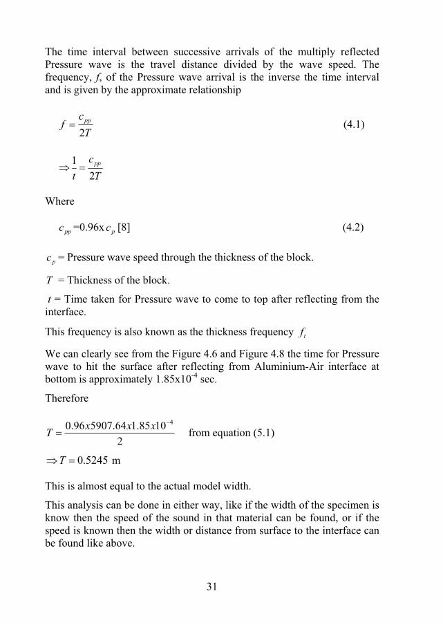
4.1.5 Results Different time domain plots were presented below with different time period ranges.
Figure 4.10. Displacement-Time plot of three response points with time range as 0 - 5x10⁻³ sec.
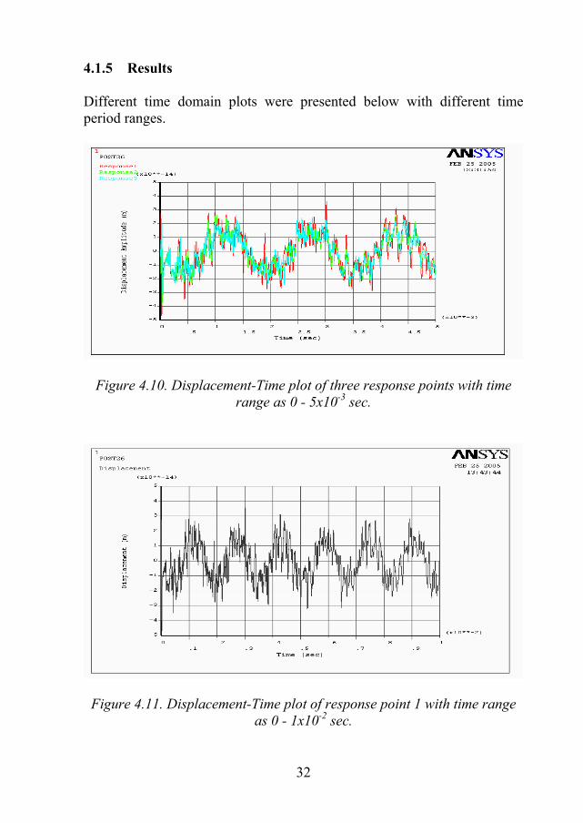
Figure 4.11. Displacement-Time plot of response point 1 with time range as 0 - 1x10⁻² sec.
32
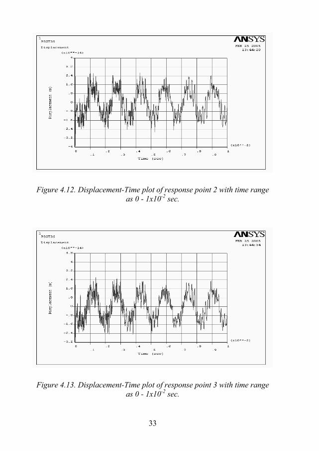
Figure 4.12. Displacement-Time plot of response point 2 with time range as 0 - 1x10⁻² sec.
Figure 4.13. Displacement-Time plot of response point 3 with time range as 0 - 1x10⁻² sec.
33
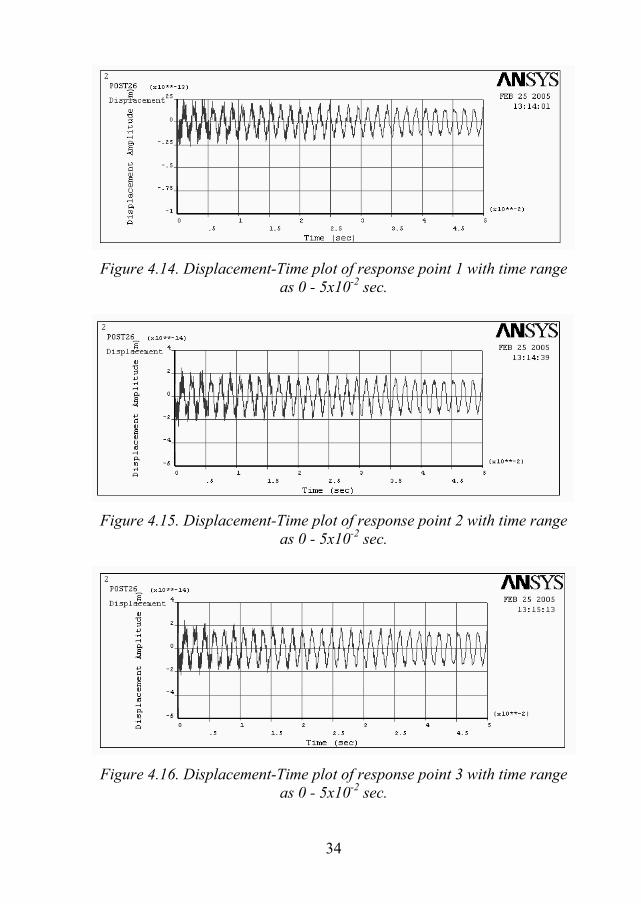
Figure 4.14. Displacement-Time plot of response point 1 with time range as 0 - 5x10⁻² sec.
Figure 4.15. Displacement-Time plot of response point 2 with time range as 0 - 5x10⁻² sec.
Figure 4.16. Displacement-Time plot of response point 3 with time range as 0 - 5x10⁻² sec.
34
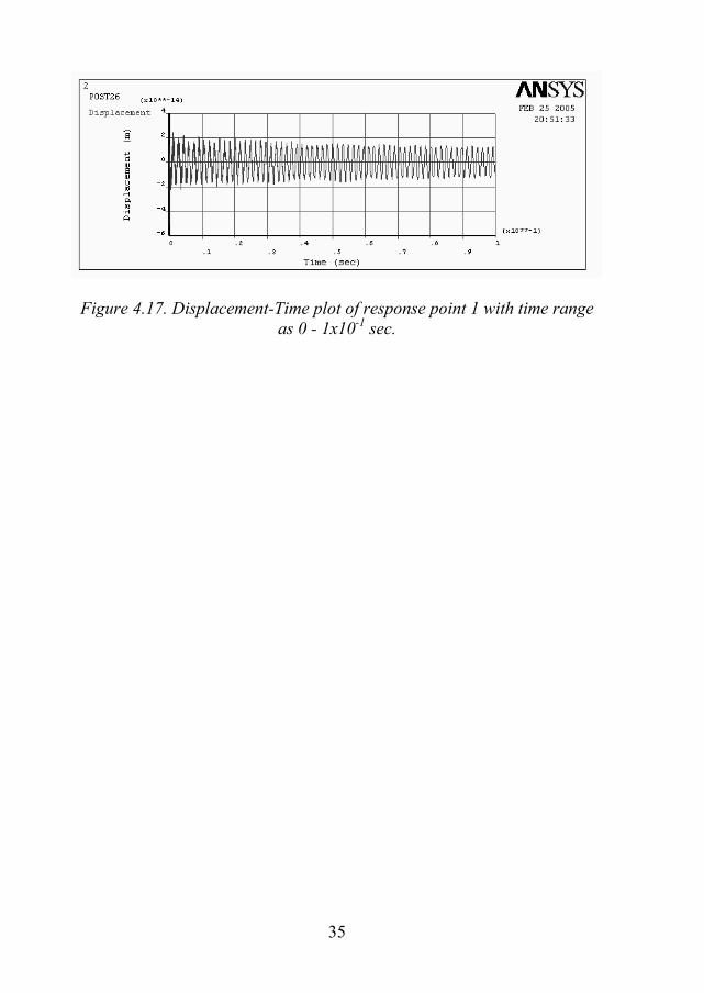
Figure 4.17. Displacement-Time plot of response point 1 with time range as 0 - 1x10⁻¹ sec.
35
4.2 Homogeneous material with crack 4.2.1 Analytical Data and Calculations
Homogeneous material is assumed as Aluminum Alloy. A small crack is modeled at a distance 0.25 m form the top and 0.5 m from the side edges. It is an elliptical shaped crack having dimensions 0.2 m major axis and 0.0001 m minor axis. Density of Aluminium (ρ) = 2700 Kg/m3
Poisson’s ratio of Aluminium (υ ) = 0.3
Young’s modulus of Aluminium (E) = 7x10¹⁰ pa
Velocity of sound in Aluminium (v) = 5907.64 m/s 4.2.2 Modeling Modeling is done using solid 82 type elements in ANSYS. To avoid the singularity near the crack tip regions this solid 82 type elements were used. Because of the elliptical shape a fine mesh is generated near crack tips. Except at the crack tips the whole model is meshed coarsely because to reduce the computer resources. Bottom extreme nodes were fixed. Finite element model of the homogeneous material with a center crack is presented below in figure 4.18.
36
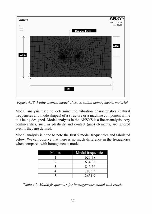
Figure 4.18. Finite element model of crack within homogeneous material.
Modal analysis used to determine the vibration characteristics (natural frequencies and mode shapes) of a structure or a machine component while it is being designed. Modal analysis in the ANSYS is a linear analysis. Any nonlinearities, such as plasticity and contact (gap) elements, are ignored even if they are defined.
Modal analysis is done to note the first 5 modal frequencies and tabulated below. We can observe that there is no much difference in the frequencies when compared with homogeneous model.
Modes Modal frequencies 1 623.78 2 634.86 3 845.56 4 1885.3 5 2631.9
Table 4.2. Modal frequencies for homogeneous model with crack.
37
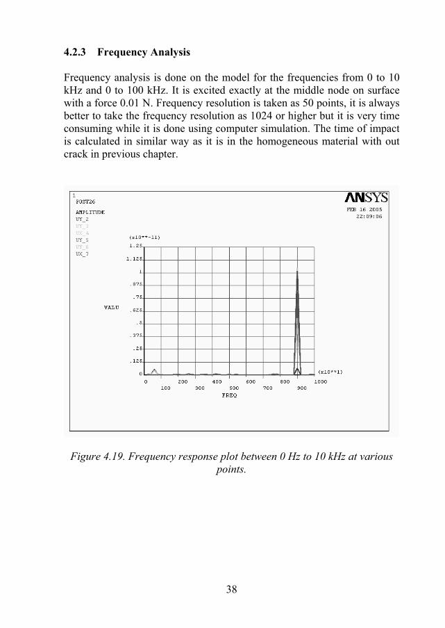
4.2.3 Frequency Analysis Frequency analysis is done on the model for the frequencies from 0 to 10 kHz and 0 to 100 kHz. It is excited exactly at the middle node on surface with a force 0.01 N. Frequency resolution is taken as 50 points, it is always better to take the frequency resolution as 1024 or higher but it is very time consuming while it is done using computer simulation. The time of impact is calculated in similar way as it is in the homogeneous material with out crack in previous chapter.
Figure 4.19. Frequency response plot between 0 Hz to 10 kHz at various points.
38
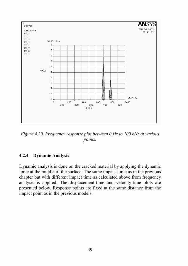
Figure 4.20. Frequency response plot between 0 Hz to 100 kHz at various
points. 4.2.4 Dynamic Analysis Dynamic analysis is done on the cracked material by applying the dynamic force at the middle of the surface. The same impact force as in the previous chapter but with different impact time as calculated above from frequency analysis is applied. The displacement-time and velocity-time plots are presented below. Response points are fixed at the same distance from the impact point as in the previous models.
39
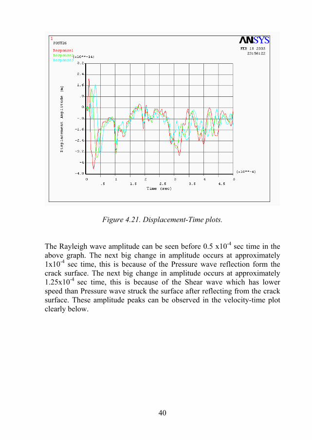
Figure 4.21. Displacement-Time plots. The Rayleigh wave amplitude can be seen before 0.5 x10⁻⁴ sec time in the above graph. The next big change in amplitude occurs at approximately 1x10⁻⁴ sec time, this is because of the Pressure wave reflection form the crack surface. The next big change in amplitude occurs at approximately 1.25x10⁻⁴ sec time, this is because of the Shear wave which has lower speed than Pressure wave struck the surface after reflecting from the crack surface. These amplitude peaks can be observed in the velocity-time plot clearly below.
40
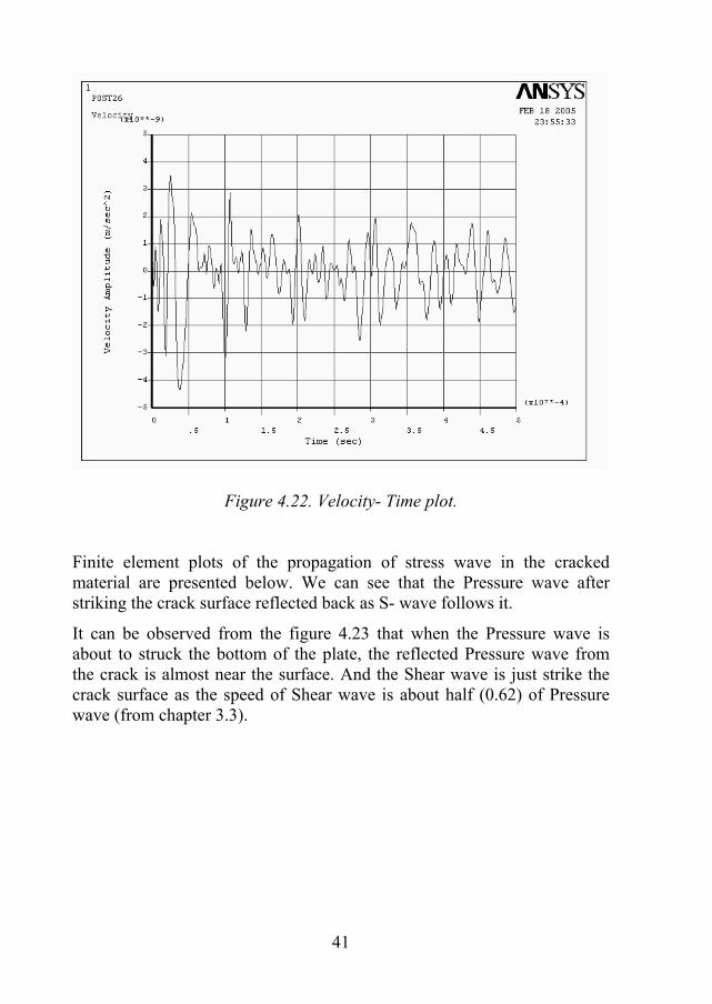
Figure 4.22. Velocity- Time plot. Finite element plots of the propagation of stress wave in the cracked material are presented below. We can see that the Pressure wave after striking the crack surface reflected back as S- wave follows it.
It can be observed from the figure 4.23 that when the Pressure wave is about to struck the bottom of the plate, the reflected Pressure wave from the crack is almost near the surface. And the Shear wave is just strike the crack surface as the speed of Shear wave is about half (0.62) of Pressure wave (from chapter 3.3).
41
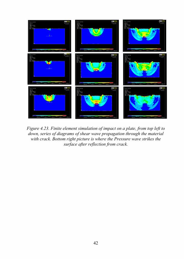
Figure 4.23. Finite element simulation of impact on a plate, from top left to down, series of diagrams of shear wave propagation through the material
with crack. Bottom right picture is where the Pressure wave strikes the surface after reflection from crack.
42
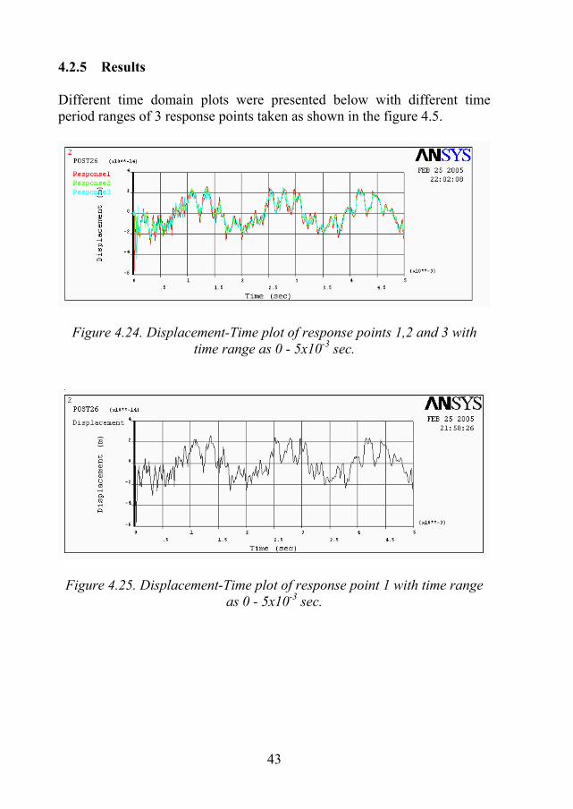
4.2.5 Results Different time domain plots were presented below with different time period ranges of 3 response points taken as shown in the figure 4.5.
Figure 4.24. Displacement-Time plot of response points 1,2 and 3 with time range as 0 - 5x10⁻³ sec.
Figure 4.25. Displacement-Time plot of response point 1 with time range as 0 - 5x10⁻³ sec.
43
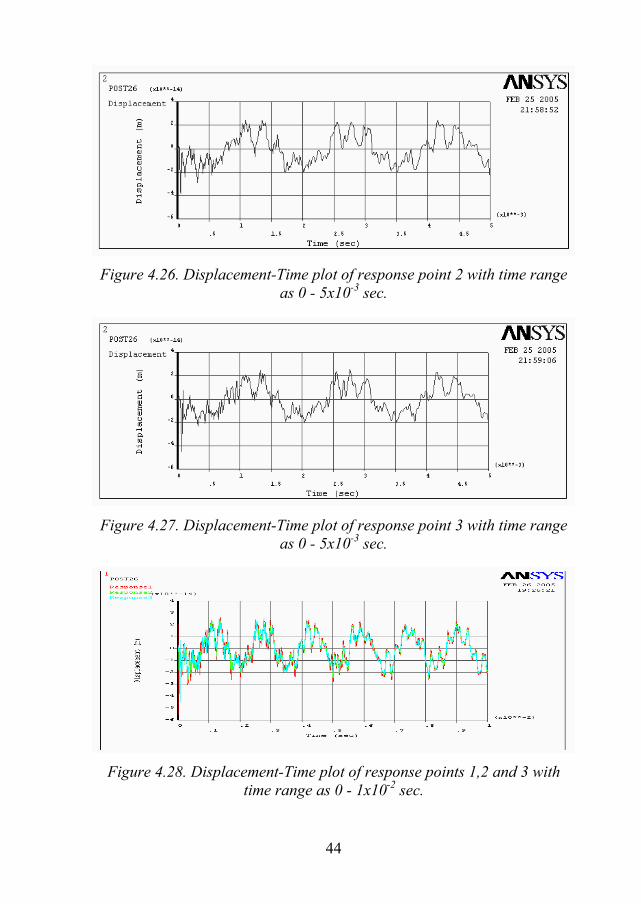
Figure 4.26. Displacement-Time plot of response point 2 with time range as 0 - 5x10⁻³ sec.
Figure 4.27. Displacement-Time plot of response point 3 with time range as 0 - 5x10⁻³ sec.
Figure 4.28. Displacement-Time plot of response points 1,2 and 3 with time range as 0 - 1x10⁻² sec.
44
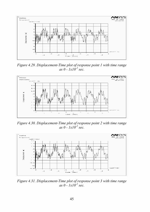
Figure 4.29. Displacement-Time plot of response point 1 with time range as 0 - 1x10⁻² sec.
Figure 4.30. Displacement-Time plot of response point 2 with time range as 0 - 1x10⁻² sec.
Figure 4.31. Displacement-Time plot of response point 3 with time range as 0 - 1x10⁻² sec.
45
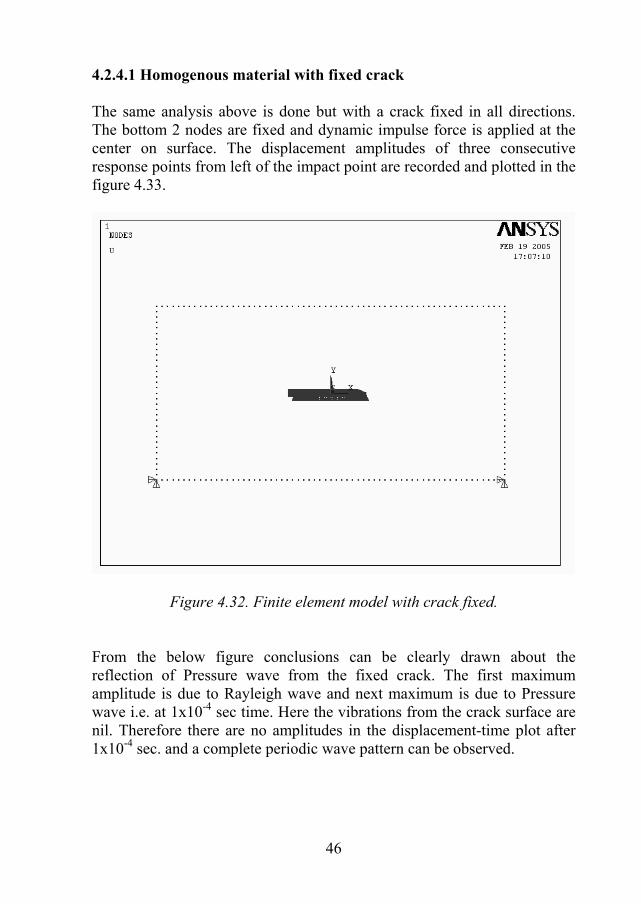
4.2.4.1 Homogenous material with fixed crack The same analysis above is done but with a crack fixed in all directions. The bottom 2 nodes are fixed and dynamic impulse force is applied at the center on surface. The displacement amplitudes of three consecutive response points from left of the impact point are recorded and plotted in the figure 4.33.
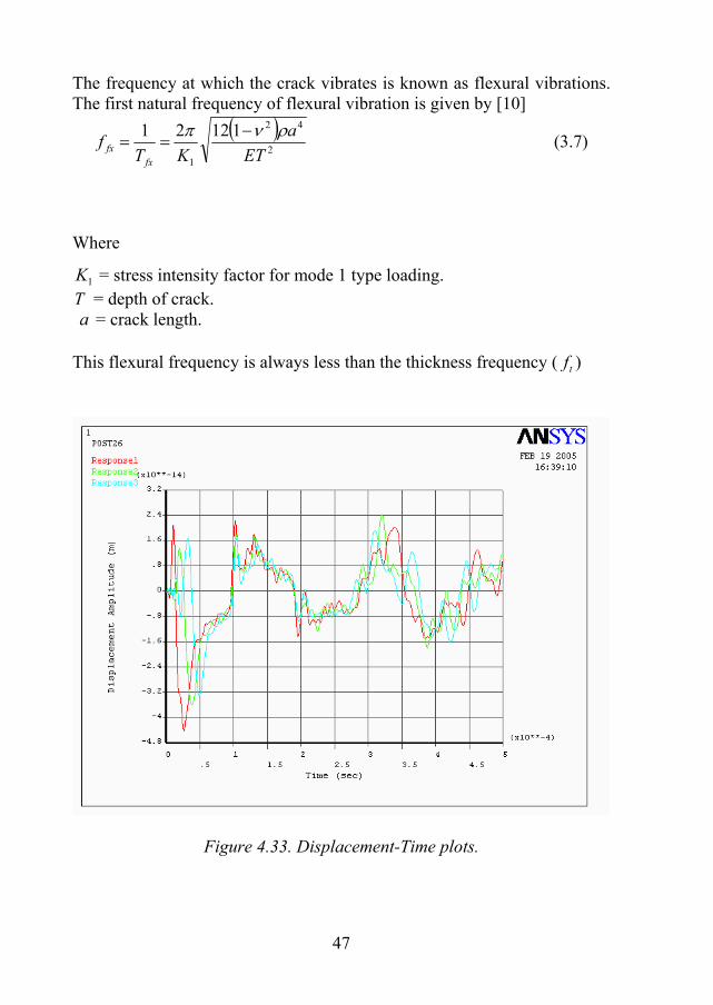
Figure 4.32. Finite element model with crack fixed. From the below figure conclusions can be clearly drawn about the reflection of Pressure wave from the fixed crack. The first maximum amplitude is due to Rayleigh wave and next maximum is due to Pressure wave i.e. at 1x10⁻⁴ sec time. Here the vibrations from the crack surface are nil. Therefore there are no amplitudes in the displacement-time plot after 1x10⁻⁴ sec. and a complete periodic wave pattern can be observed.
46
The frequency at which the crack vibrates is known as flexural vibrations. The first natural frequency of flexural vibration is given by [10]
( )2
42
1
11221ET
aKT
ffx
fxρνπ −
== (3.7)
Where
1K = stress intensity factor for mode 1 type loading. T = depth of crack. = crack length. a This flexural frequency is always less than the thickness frequency ( ) tf
Figure 4.33. Displacement-Time plots.
47
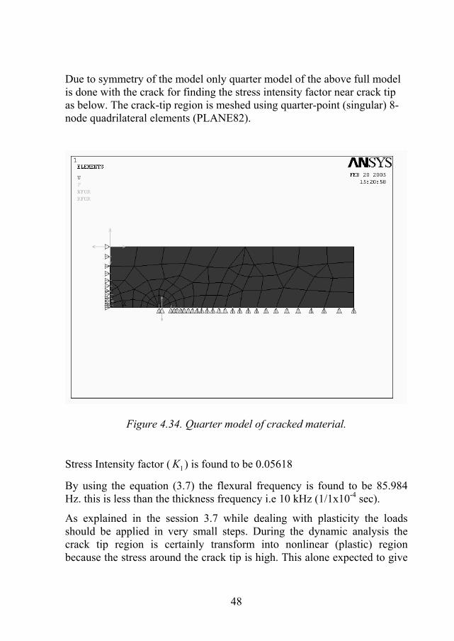
Due to symmetry of the model only quarter model of the above full model is done with the crack for finding the stress intensity factor near crack tip as below. The crack-tip region is meshed using quarter-point (singular) 8-node quadrilateral elements (PLANE82).
Figure 4.34. Quarter model of cracked material. Stress Intensity factor ( ) is found to be 0.05618 1K
By using the equation (3.7) the flexural frequency is found to be 85.984 Hz. this is less than the thickness frequency i.e 10 kHz (1/1x10-4 sec).
As explained in the session 3.7 while dealing with plasticity the loads should be applied in very small steps. During the dynamic analysis the crack tip region is certainly transform into nonlinear (plastic) region because the stress around the crack tip is high. This alone expected to give
48
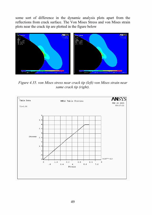
some sort of difference in the dynamic analysis plots apart from the reflections from crack surface. The Von Mises Stress and von Mises strain plots near the crack tip are plotted in the figure below
Figure 4.35. von Mises stress near crack tip (left) von Mises strain near same crack tip (right).
49
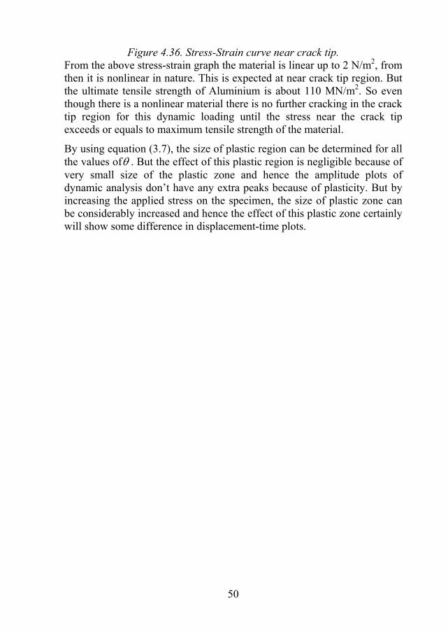
Figure 4.36. Stress-Strain curve near crack tip. From the above stress-strain graph the material is linear up to 2 N/m2, from then it is nonlinear in nature. This is expected at near crack tip region. But the ultimate tensile strength of Aluminium is about 110 MN/m2. So even though there is a nonlinear material there is no further cracking in the crack tip region for this dynamic loading until the stress near the crack tip exceeds or equals to maximum tensile strength of the material.
By using equation (3.7), the size of plastic region can be determined for all the values ofθ . But the effect of this plastic region is negligible because of very small size of the plastic zone and hence the amplitude plots of dynamic analysis don’t have any extra peaks because of plasticity. But by increasing the applied stress on the specimen, the size of plastic zone can be considerably increased and hence the effect of this plastic zone certainly will show some difference in displacement-time plots.
50
4.3 Heterogeneous material 4.3.1 Analytical Data and Calculations Heterogeneous material is assumed as the combination of Aluminium and Low Carbon Steel which is AISI 1000 Series Steel with the following material properties [9]
Material properties low carbon steel:
Density of steel (ρ) = 7872 Kg/m3
Poisson’s ratio of steel (υ ) = 0.29 Young’s modulus of steel (E) = 2x10¹¹ pa Velocity of sound in steel ( v ) is calculated form the equation (3.2) as
v =))(ρ(
)E(c p υυυ
2111
−+−
= = )29.021)(29.01(7872
)29.01(102 11
xx
−+− = 5770.08 m/s
Material properties of aluminium:
Density of Aluminium (ρ) = 2700 Kg/m3
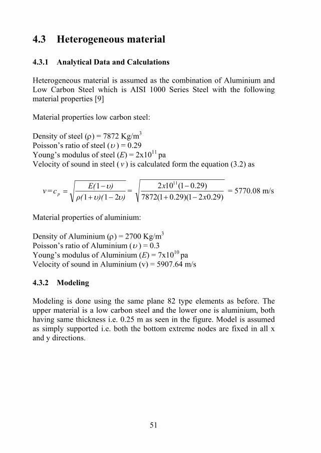
Poisson’s ratio of Aluminium (υ ) = 0.3 Young’s modulus of Aluminium (E) = 7x10¹⁰ pa Velocity of sound in Aluminium (v) = 5907.64 m/s 4.3.2 Modeling Modeling is done using the same plane 82 type elements as before. The upper material is a low carbon steel and the lower one is aluminium, both having same thickness i.e. 0.25 m as seen in the figure. Model is assumed as simply supported i.e. both the bottom extreme nodes are fixed in all x and y directions.
51
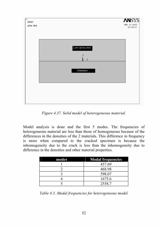
Figure 4.37. Solid model of heterogeneous material. Model analysis is done and the first 5 modes. The frequencies of heterogeneous material are less than those of homogeneous because of the differences in the densities of the 2 materials. This difference in frequency is more when compared to the cracked specimen is because the inhomogeneity due to the crack is less than the inhomogeneity due to difference in the densities and other material properties.
modes Modal frequencies 1 457.69 2 468.98 3 598.07 4 1675.6 5 2558.7
Table 4.3. Modal frequencies for heterogeneous model.
52
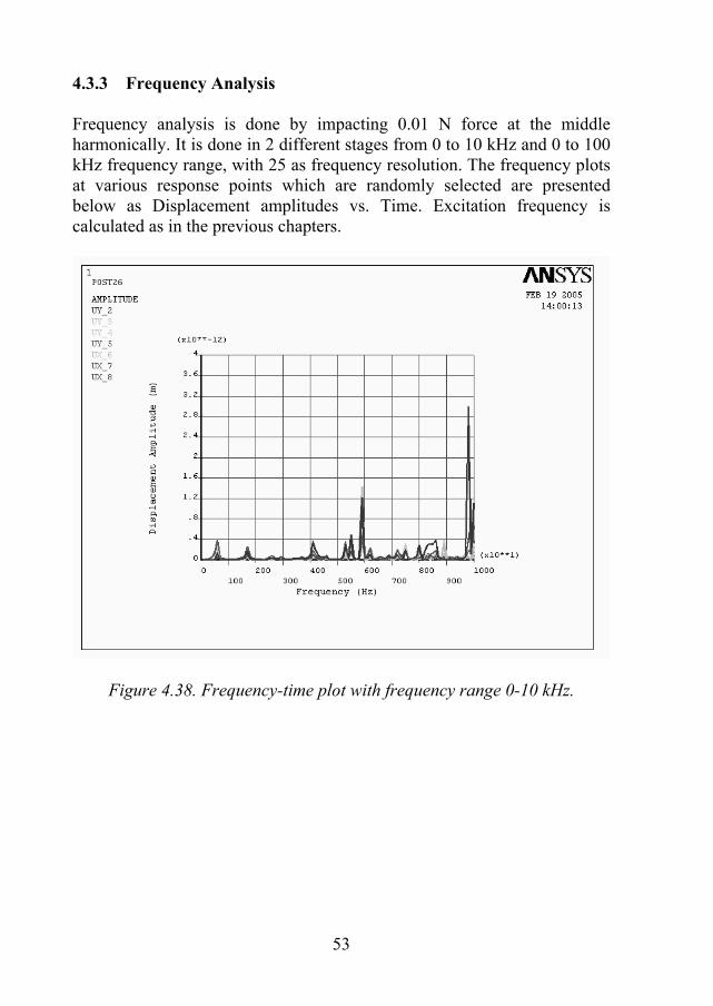
4.3.3 Frequency Analysis Frequency analysis is done by impacting 0.01 N force at the middle harmonically. It is done in 2 different stages from 0 to 10 kHz and 0 to 100 kHz frequency range, with 25 as frequency resolution. The frequency plots at various response points which are randomly selected are presented below as Displacement amplitudes vs. Time. Excitation frequency is calculated as in the previous chapters.
Figure 4.38. Frequency-time plot with frequency range 0-10 kHz.
53
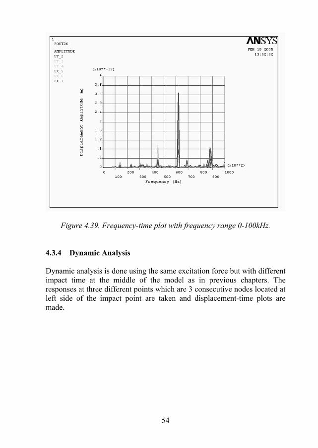
Figure 4.39. Frequency-time plot with frequency range 0-100kHz. 4.3.4 Dynamic Analysis Dynamic analysis is done using the same excitation force but with different impact time at the middle of the model as in previous chapters. The responses at three different points which are 3 consecutive nodes located at left side of the impact point are taken and displacement-time plots are made.
54
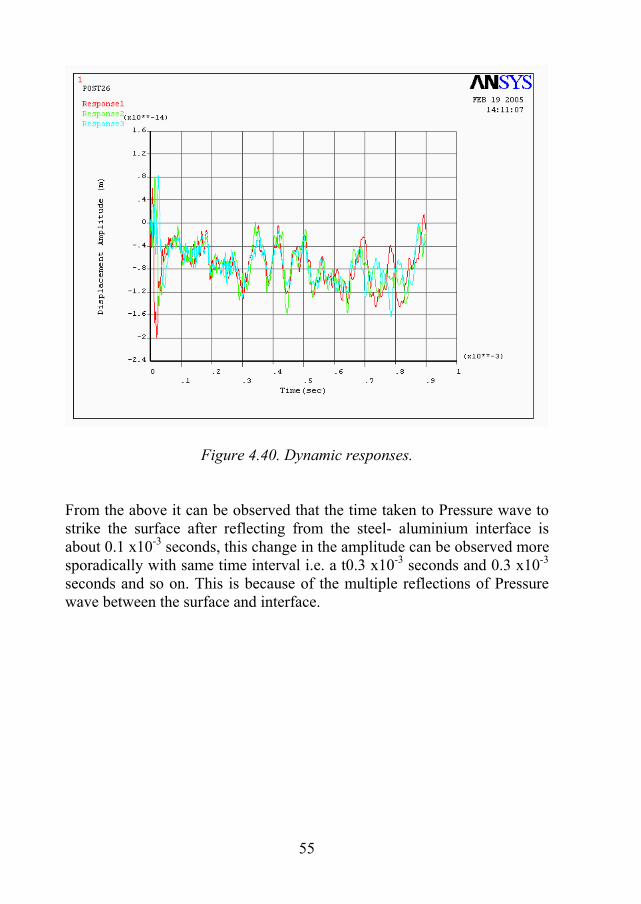
Figure 4.40. Dynamic responses. From the above it can be observed that the time taken to Pressure wave to strike the surface after reflecting from the steel- aluminium interface is about 0.1 x10⁻³ seconds, this change in the amplitude can be observed more sporadically with same time interval i.e. a t0.3 x10-3 seconds and 0.3 x10⁻³ seconds and so on. This is because of the multiple reflections of Pressure wave between the surface and interface.
55
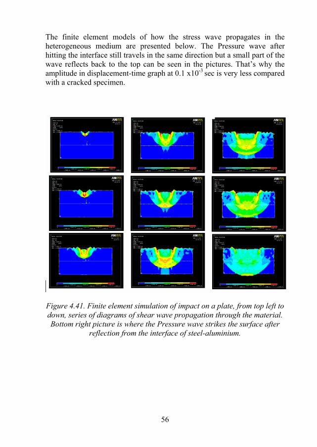
The finite element models of how the stress wave propagates in the heterogeneous medium are presented below. The Pressure wave after hitting the interface still travels in the same direction but a small part of the wave reflects back to the top can be seen in the pictures. That’s why the amplitude in displacement-time graph at 0.1 x10⁻³ sec is very less compared with a cracked specimen.
Figure 4.41. Finite element simulation of impact on a plate, from top left to down, series of diagrams of shear wave propagation through the material. Bottom right picture is where the Pressure wave strikes the surface after
reflection from the interface of steel-aluminium.
56
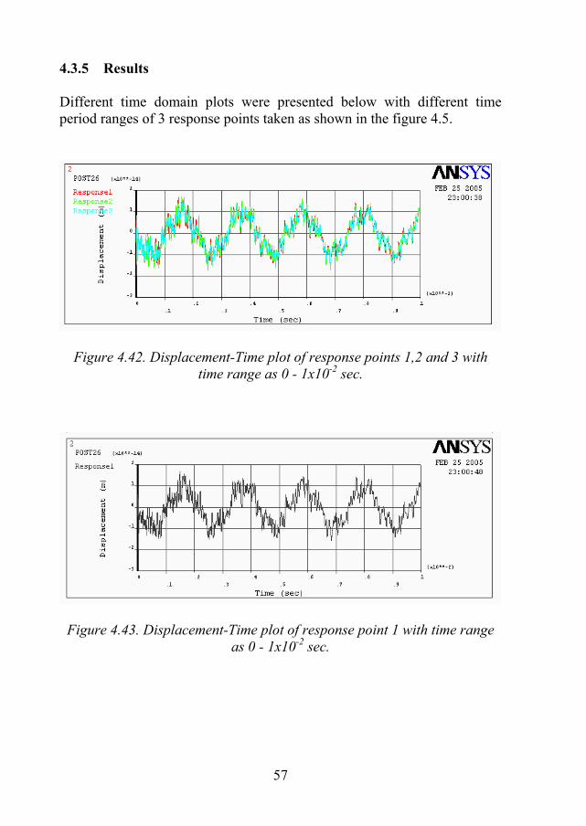
4.3.5 Results Different time domain plots were presented below with different time period ranges of 3 response points taken as shown in the figure 4.5.
Figure 4.42. Displacement-Time plot of response points 1,2 and 3 with time range as 0 - 1x10⁻² sec.
Figure 4.43. Displacement-Time plot of response point 1 with time range as 0 - 1x10⁻² sec.
57
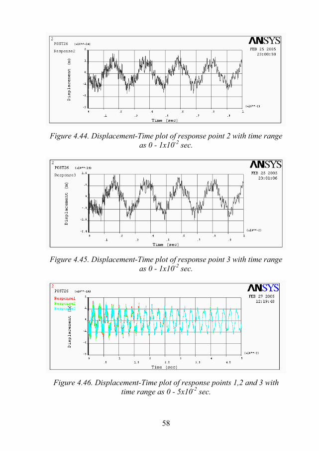
Figure 4.44. Displacement-Time plot of response point 2 with time range as 0 - 1x10⁻² sec.
Figure 4.45. Displacement-Time plot of response point 3 with time range as 0 - 1x10⁻² sec.
Figure 4.46. Displacement-Time plot of response points 1,2 and 3 with time range as 0 - 5x10⁻² sec.
58
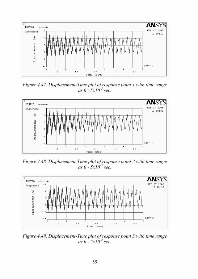
Figure 4.47. Displacement-Time plot of response point 1 with time range as 0 - 5x10⁻² sec.
Figure 4.48. Displacement-Time plot of response point 2 with time range as 0 - 5x10⁻² sec.
Figure 4.49. Displacement-Time plot of response point 3 with time range as 0 - 5x10⁻² sec.
59
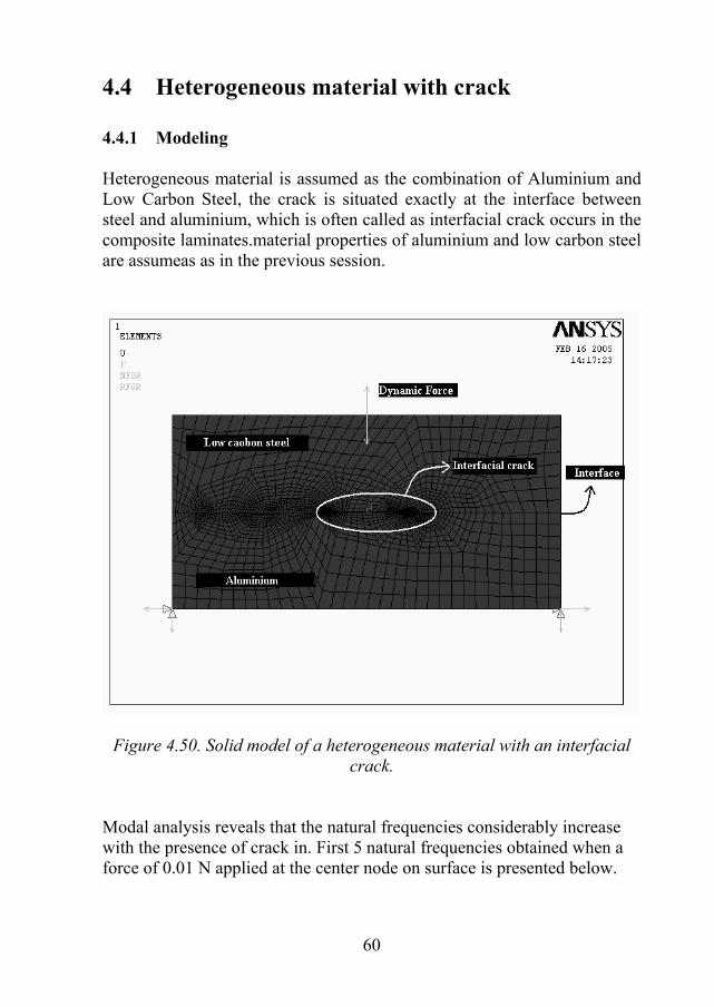
4.4 Heterogeneous material with crack 4.4.1 Modeling Heterogeneous material is assumed as the combination of Aluminium and Low Carbon Steel, the crack is situated exactly at the interface between steel and aluminium, which is often called as interfacial crack occurs in the composite laminates.material properties of aluminium and low carbon steel are assumeas as in the previous session.
Figure 4.50. Solid model of a heterogeneous material with an interfacial crack.
Modal analysis reveals that the natural frequencies considerably increase with the presence of crack in. First 5 natural frequencies obtained when a force of 0.01 N applied at the center node on surface is presented below.
60
modes Modal frequencies 1 709.58 2 718.39 3 1104.2 4 1928.6 5 2610.7
Table 4.4. Modal frequencies for model with crack.
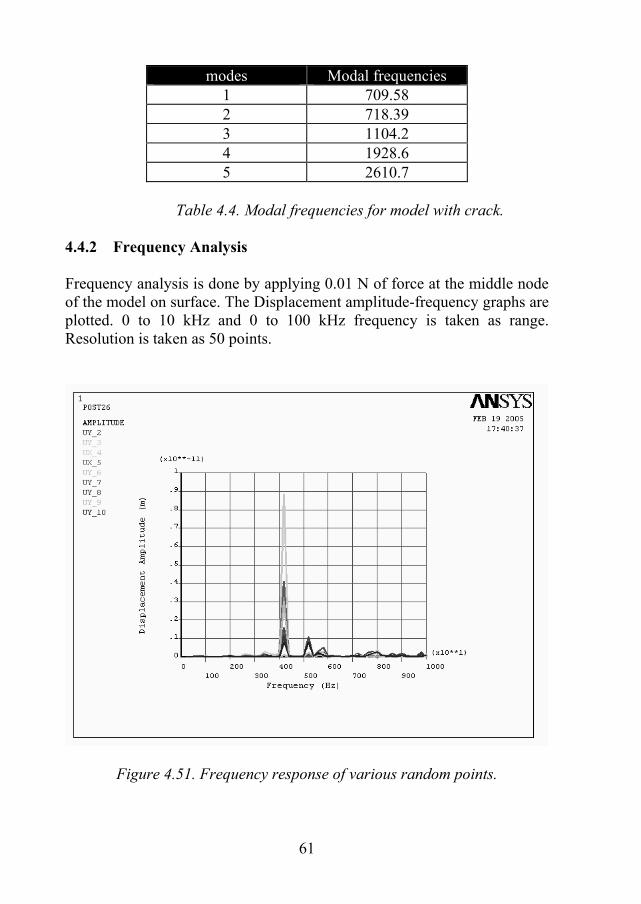
4.4.2 Frequency Analysis Frequency analysis is done by applying 0.01 N of force at the middle node of the model on surface. The Displacement amplitude-frequency graphs are plotted. 0 to 10 kHz and 0 to 100 kHz frequency is taken as range. Resolution is taken as 50 points.
Figure 4.51. Frequency response of various random points.
61
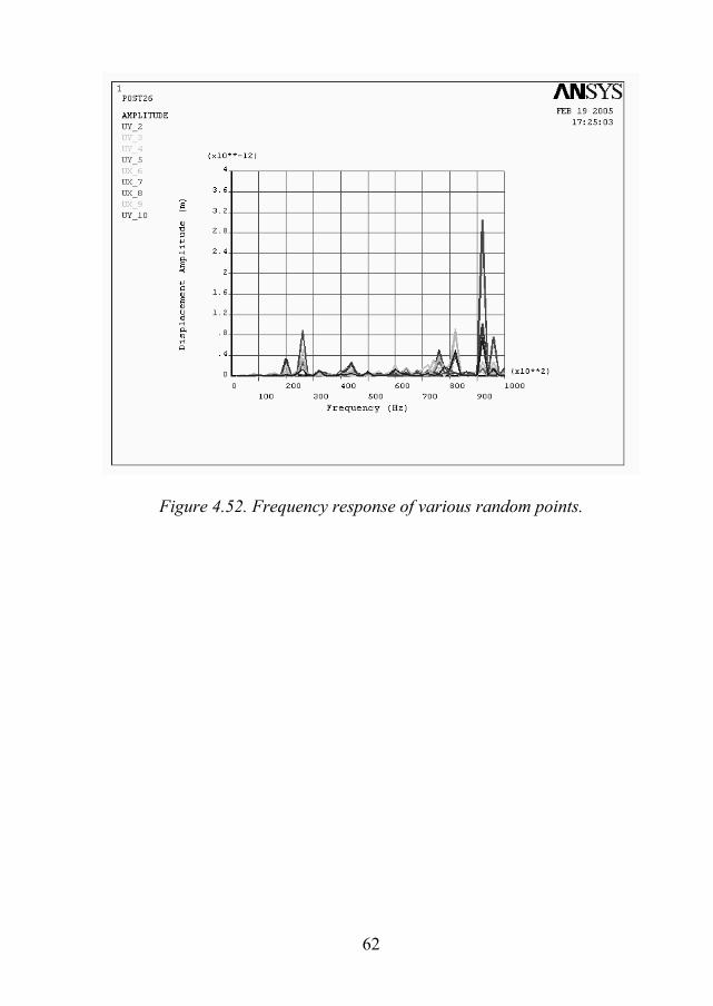
Figure 4.52. Frequency response of various random points.
62
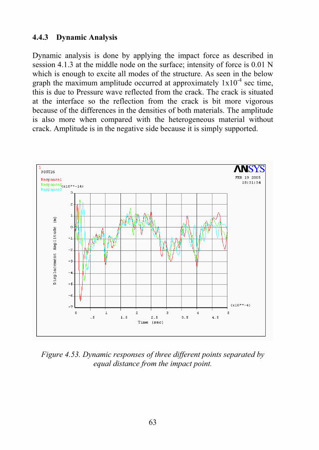
4.4.3 Dynamic Analysis Dynamic analysis is done by applying the impact force as described in session 4.1.3 at the middle node on the surface; intensity of force is 0.01 N which is enough to excite all modes of the structure. As seen in the below graph the maximum amplitude occurred at approximately 1x10⁻⁴ sec time, this is due to Pressure wave reflected from the crack. The crack is situated at the interface so the reflection from the crack is bit more vigorous because of the differences in the densities of both materials. The amplitude is also more when compared with the heterogeneous material without crack. Amplitude is in the negative side because it is simply supported.
Figure 4.53. Dynamic responses of three different points separated by equal distance from the impact point.
63
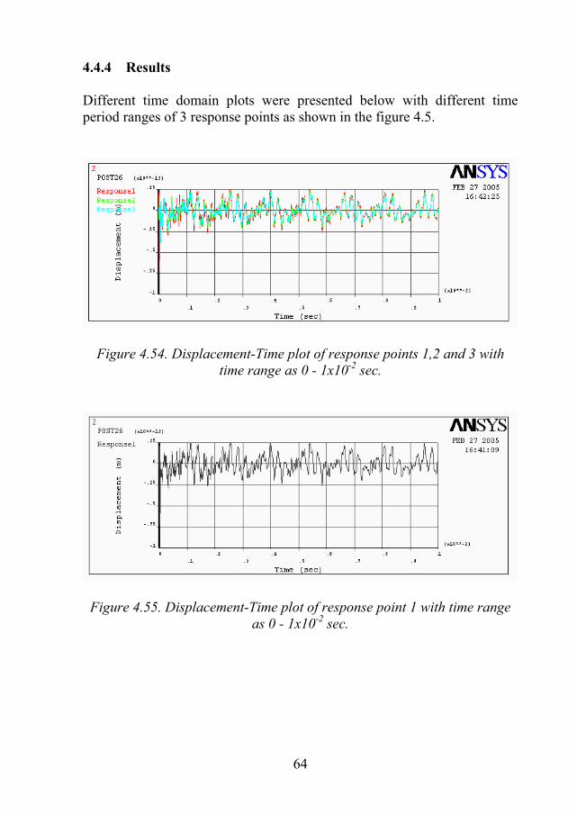
4.4.4 Results Different time domain plots were presented below with different time period ranges of 3 response points as shown in the figure 4.5.
Figure 4.54. Displacement-Time plot of response points 1,2 and 3 with time range as 0 - 1x10⁻² sec.
Figure 4.55. Displacement-Time plot of response point 1 with time range as 0 - 1x10⁻² sec.
64
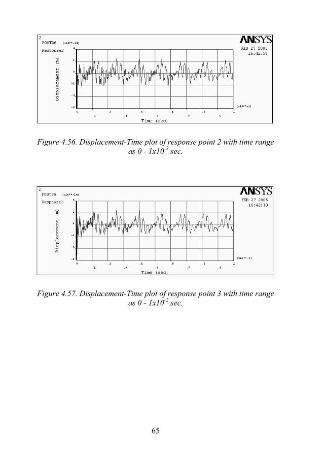
Figure 4.56. Displacement-Time plot of response point 2 with time range as 0 - 1x10⁻² sec.
Figure 4.57. Displacement-Time plot of response point 3 with time range as 0 - 1x10⁻² sec.
65
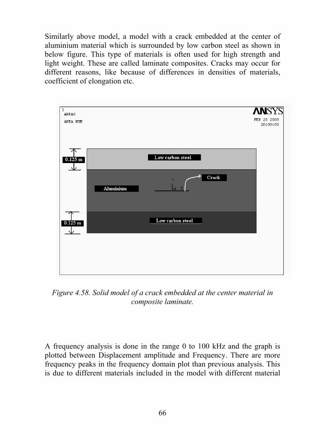
Similarly above model, a model with a crack embedded at the center of aluminium material which is surrounded by low carbon steel as shown in below figure. This type of materials is often used for high strength and light weight. These are called laminate composites. Cracks may occur for different reasons, like because of differences in densities of materials, coefficient of elongation etc.
Figure 4.58. Solid model of a crack embedded at the center material in composite laminate.
A frequency analysis is done in the range 0 to 100 kHz and the graph is plotted between Displacement amplitude and Frequency. There are more frequency peaks in the frequency domain plot than previous analysis. This is due to different materials included in the model with different material
66
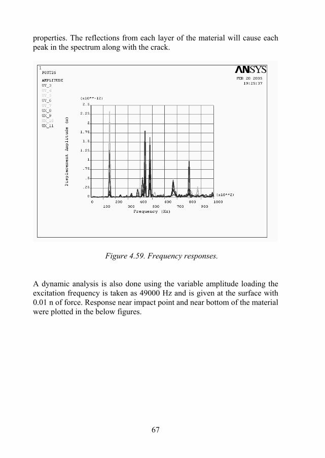
properties. The reflections from each layer of the material will cause each peak in the spectrum along with the crack.
Figure 4.59. Frequency responses. A dynamic analysis is also done using the variable amplitude loading the excitation frequency is taken as 49000 Hz and is given at the surface with 0.01 n of force. Response near impact point and near bottom of the material were plotted in the below figures.
67
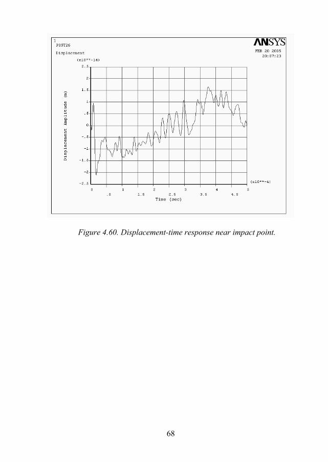
Figure 4.60. Displacement-time response near impact point.
68
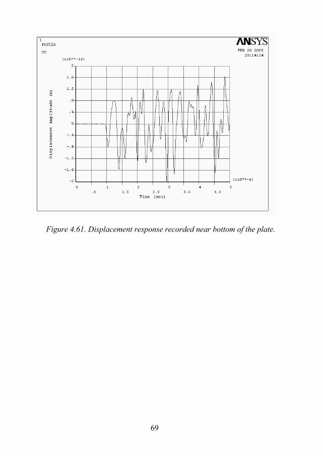
Figure 4.61. Displacement response recorded near bottom of the plate.
69
5 Conclusions Dynamic analysis is a very important investigation when it comes to the composite materials, where these can exhibit diversity in material properties as well as shapes. The main idea of this work is to perform dynamic analysis which gives the information about various factors including cracks, voids, interfaces and the locations of the damages etc. on different types of materials ranging from normal homogeneous material to complex composite laminates.
In real life situations doing a dynamic analysis on structures requires great skill and experience, because the excitation force which is dynamically given on the structure should be chosen very carefully and the excitation point is also plays very important role in dynamic analysis. By doing the computer simulation of dynamic analysis gives us the variety in choosing excitation signal as well as the excitation points.
In this work the modal analysis is done on different types of materials for finding modal frequencies which are very useful to do the frequency analysis which requires the range of frequencies in the system vibrates more (natural frequencies). After doing the frequency analysis the next step is to perform a static analysis or dynamic analysis depending on the requirement. Finding the damages in the materials is of course a very important non-destructive testing which dealt with ease here with computer simulation by using dynamic analysis. Not only finding the damages but the location of damages is always required in process, this is also done here by plotting the Displacement-Time curves for different types of materials and examining the plots by using basic formulas. Time axis is adjusted for different values from 5x10⁻⁴ seconds to 0.1 seconds and the displacement response is documented for analyzing the after effects in the vibrations of different types of materials with different damage locations. It is perceived that there are many things to be noticed from those plots and further work certainly needed to distinguish the differences in each plot.
70
6 Further approach to work This work leads to very appealing thoughts about dynamic analysis. This work is carried out to find the fracture location. But the type of damages range from fractures to debonds and plasticity etc. Modeling debonds and delaminations and doing the dynamic analysis and finding the type of damage can be done further to extend this work. Here in this work the materials used are very dirt free and hygienic i.e. apart from the fracture there are no damages in the materials, in real life situations can be encountered with many unclear materials like concrete structures with air filled voids every where, steel bridges with so many cracks, this work will certainly help in those types of situations where a small part of the structure is to be examined. But doing analysis for the whole structure is often required. There are many factors concerned with fractures differs when the dynamic time plots were extended to higher time values, which is of course done here for variety of materials, but those factors should be accounted for higher studies in this perspective.
71
7 References 1. Fatemi, A., and Yang, L, (1998), “Cumulative Fatigue Damage and
Life Prediction Theories: A Survey of the State of the Art for Homogeneous Materials,” International Journal of Fatigue, Vol. 20, No. 1, pp 9-34.
2. T.L. Anderson., (1995), “Fracrure mechanics: Fundamentals and Applications”, 2nd Ed, pp 12-18.
3. ANSYS Documentation
4. Tada, H., Paris P. C., and Irwin, G. T., (2000), The Stress Analysis of Cracks Handbook, 3rd Ed., U.S.A.
5. Krautkrämer, J. and Krautkrämer, H.,(1990), Ultrasonic Testing of Materials, 4th Ed., Springer- Verlag, U.S.A.
6. Sansalone, M. and Carino, N.J., (1991), “Stress Wave Propagation Methods,” in Handbook on Nondestructive Testing of Concrete, Ed. V.M. Malhotra and N.J. Carino, pp. 275-304.
7. Sansalone, M., and Carino, N.J., (1986), “Impact-Echo: A Method for Flaw Detection in Concrete Using Transient Stress Waves,” NBSIR 86-3452, National Bureau of Standards, Sept., 222 p.
8. Lin, J. M., and Sansalone, M., (1997), “A Procedure for Determining Pressure wave Speed in Concrete for Use in Impact-Echo Testing Using a Rayleigh Wave Speed Measurement Technique,” Innovations in Nondestructive Testing, SP-168, S. Pessiki and L. Olson, Eds., American Concrete Institute, Farmington Hills, MI, pp.137-165
9. http://www.matweb.com/iqy/iqysample.com (21/2/2005)
10. Meirovitch L., (1986), Elements of vibration analysis. McGrawhill.
72
Appendices A. Code for dynamic analysis of homogeneous material. A=0.01 ! 0.01 N force xtime=0.000010204 ! one period in seconds asize=25 ! data resolution pi=3.141592654 *dim,xdata,array,asize,2,1,time xdata(1,1,1)=0.001 xdata(1,2,1)=0.0 *do,i,2,asize xfr=pi*(i/asize) xdata(i,1)=i ! time xdata(i,2)=(A*sin(xfr)) ! data *enddo /CONFIG,NRES,10000 !!!!Full Transient Analysis!!!! /SOLU !* ANTYPE,4 TRNOPT,FULL outres,all,all !* *do,i,2,25 nsel,s,NODE,,1542 F,all,fy,-xdata(i,2) ! from input define above TIME,(xtime/asize)*i AUTOTS,on deltim,xtime/asize ! ITS KBC,0 allsel,all solve *enddo
73
nsel,s,NODE,,1542 F,all,fy,0 ! ending the input TIME,0.000010205 AUTOTS,on deltim,xtime/asize ! ITS KBC,0 allsel,all solve !* nsel,s,NODE,,1542 F,all,fy,0 ! prolonging the input to 0.01 sec TIME,0.01 AUTOTS,on deltim,xtime/10 ! ITS KBC,0 allsel,all solve /POST26 numvar,200, NSOL,2,1542,U,y,Displacement !COMPUTE DISPLACEMENTS DERIV,3,2,,,Velocity ! COMPUTE VELOCITIES DERIV,4,3,,,Acceleration !COMPUTE ACCELERATIONS NSOL,5,404,U,y,Displacement !COMPUTE DISPLACEMENTS DERIV,6,5,,,Velocity ! COMPUTE VELOCITIES DERIV,7,6,,,Acceleration !COMPUTE ACCELERATIONS NSOL,8,402,U,y,Displacement !COMPUTE DISPLACEMENTS DERIV,9,8,,,Velocity ! COMPUTE VELOCITIES DERIV,10,9,,,Acceleration !COMPUTE ACCELERATIONS NSOL,11,400,U,y,Displacement !COMPUTE DISPLACEMENTS DERIV,12,11,,,Velocity ! COMPUTE VELOCITIES DERIV,13,12,,,Acceleration !COMPUTE ACCELERATIONS ! PLVAR,2,3,4, , , , , , , , /gropts,view,1 !* finish /post1
74
B. Code for dynamic analysis of homogeneous material with crack. A=0.01 ! 0.01 newtons force xtime=0.000010204 ! seconds asize=25 ! data resolution pi=3.141592654 *dim,xdata,array,asize,2,1,time xdata(1,1,1)=0.001 xdata(1,2,1)=0.0 *do,i,2,asize xfr=pi*(i/asize) xdata(i,1)=i ! time xdata(i,2)=(A*sin(xfr)) ! data *enddo /CONFIG,NRES,20000 !!!!Full Transient Analysis!!!! /SOLU !* ANTYPE,4 TRNOPT,FULL outres,all,all !* *do,i,2,25 nsel,s,NODE,,21326 F,all,fy,-xdata(i,2) ! from input define above TIME,(xtime/asize)*i AUTOTS,on deltim,xtime/asize ! ITS KBC,0 allsel,all solve *enddo nsel,s,NODE,,21326 F,all,fy,0 ! ending the input TIME,0.000010205
75
AUTOTS,on deltim,xtime/asize ! ITS KBC,0 allsel,all solve !* nsel,s,NODE,,21326 F,all,fy,0 ! prolonging the input to 0.03 sec TIME,0.03 AUTOTS,on deltim,xtime ! ITS KBC,0 allsel,all solve /POST26 numvar,200, NSOL,2,21326,U,y,Displacement !COMPUTE DISPLACEMENTS DERIV,3,2,,,Velocity ! COMPUTE VELOCITIES DERIV,4,3,,,Acceleration !COMPUTE ACCELERATIONS NSOL,5,1610,U,y,Displacement !COMPUTE DISPLACEMENTS DERIV,6,5,,,Velocity ! COMPUTE VELOCITIES DERIV,7,6,,,Acceleration !COMPUTE ACCELERATIONS NSOL,8,1606,U,y,Displacement !COMPUTE DISPLACEMENTS DERIV,9,8,,,Velocity ! COMPUTE VELOCITIES DERIV,10,9,,,Acceleration !COMPUTE ACCELERATIONS NSOL,11,1604,U,y,Displacement !COMPUTE DISPLACEMENTS DERIV,12,11,,,Velocity ! COMPUTE VELOCITIES DERIV,13,12,,,Acceleration !COMPUTE ACCELERATIONS ! PLVAR,2,3,4, , , , , , , , /gropts,view,1 !* finish /post1
76
C. Code for dynamic analysis of heterogeneous material. A=0.01 ! 0.01 newtons force xtime=0.000010204 ! seconds asize=25 ! data resolution pi=3.141592654 *dim,xdata,array,asize,2,1,time xdata(1,1,1)=0.001 xdata(1,2,1)=0.0 *do,i,2,asize xfr=pi*(i/asize) xdata(i,1)=i ! time xdata(i,2)=(A*sin(xfr)) ! data *enddo /CONFIG,NRES,10000 !!!!Full Transient Analysis!!!! /SOLU !* ANTYPE,4 TRNOPT,FULL outres,all,all !* *do,i,2,25 nsel,s,NODE,,1512 F,all,fy,-xdata(i,2) ! from input define above TIME,(xtime/asize)*i AUTOTS,on deltim,xtime/asize ! ITS KBC,0 allsel,all solve *enddo nsel,s,NODE,,1512 F,all,fy,0 ! ending the input TIME,0.000010205
77

AUTOTS,on deltim,xtime/asize ! ITS KBC,0 allsel,all solve !* nsel,s,NODE,,1512 F,all,fy,0 ! prolonging the input to 0.05 sec TIME,0.05 AUTOTS,on deltim,xtime/10 ! ITS KBC,0 allsel,all solve /POST26 numvar,200, NSOL,2,1512,U,y,Displacement !COMPUTE DISPLACEMENTS DERIV,3,2,,,Velocity ! COMPUTE VELOCITIES DERIV,4,3,,,Acceleration !COMPUTE ACCELERATIONS NSOL,5,1507,U,y,Displacement !COMPUTE DISPLACEMENTS DERIV,6,5,,,Velocity ! COMPUTE VELOCITIES DERIV,7,6,,,Acceleration !COMPUTE ACCELERATIONS NSOL,8,182,U,y,Displacement !COMPUTE DISPLACEMENTS DERIV,9,8,,,Velocity ! COMPUTE VELOCITIES DERIV,10,9,,,Acceleration !COMPUTE ACCELERATIONS NSOL,11,176,U,y,Displacement !COMPUTE DISPLACEMENTS DERIV,12,11,,,Velocity ! COMPUTE VELOCITIES DERIV,13,12,,,Acceleration !COMPUTE ACCELERATIONS ! PLVAR,2,3,4, , , , , , , , /gropts,view,1 !* finish /post1
78
D. Code for dynamic analysis of heterogeneous material with crack. A=0.01 ! 0.01 newtons force xtime=0.000010204 ! seconds asize=25 ! data resolution pi=3.141592654 *dim,xdata,array,asize,2,1,time xdata(1,1,1)=0.001 xdata(1,2,1)=0.0 *do,i,2,asize xfr=pi*(i/asize) xdata(i,1)=i ! time xdata(i,2)=(A*sin(xfr)) ! data *enddo /CONFIG,NRES,10000 !!!!Full Transient Analysis!!!! /SOLU !* ANTYPE,4 TRNOPT,FULL outres,all,all !* *do,i,2,25 nsel,s,NODE,,8875 F,all,fy,-xdata(i,2) ! from input define above TIME,(xtime/asize)*i AUTOTS,on deltim,xtime/asize ! ITS KBC,0 allsel,all solve *enddo nsel,s,NODE,,8875 F,all,fy,0 ! ending the input
79
TIME,0.000010205 AUTOTS,on deltim,xtime/asize ! ITS KBC,0 allsel,all solve !* nsel,s,NODE,,8875 F,all,fy,0 ! prolonging the input to 0.01 sec TIME,0.01 AUTOTS,on deltim,xtime ! ITS KBC,0 allsel,all solve /POST26 numvar,200, NSOL,2,8875,U,y,Displacement !COMPUTE DISPLACEMENTS DERIV,3,2,,,Velocity ! COMPUTE VELOCITIES DERIV,4,3,,,Acceleration !COMPUTE ACCELERATIONS NSOL,5,2816,U,y,Displacement !COMPUTE DISPLACEMENTS DERIV,6,5,,,Velocity ! COMPUTE VELOCITIES DERIV,7,6,,,Acceleration !COMPUTE ACCELERATIONS NSOL,8,2804,U,y,Displacement !COMPUTE DISPLACEMENTS DERIV,9,8,,,Velocity ! COMPUTE VELOCITIES DERIV,10,9,,,Acceleration !COMPUTE ACCELERATIONS NSOL,11,2800,U,y,Displacement !COMPUTE DISPLACEMENTS DERIV,12,11,,,Velocity ! COMPUTE VELOCITIES DERIV,13,12,,,Acceleration !COMPUTE ACCELERATIONS ! PLVAR,2,3,4, , , , , , , , /gropts,view,1 !* finish /post1
80
E. Code for dynamic analysis of composite laminate material with embedded crack.
A=0.01 ! 0.01 newtons force xtime=0.000010204 ! seconds asize=25 ! data resolution pi=3.141592654 *dim,xdata,array,asize,2,1,time xdata(1,1,1)=0.001 xdata(1,2,1)=0.0 *do,i,2,asize xfr=pi*(i/asize) xdata(i,1)=i ! time xdata(i,2)=(A*sin(xfr)) ! data *enddo !!!!Full Transient Analysis!!!! /SOLU !* ANTYPE,4 TRNOPT,FULL outres,all,all !* *do,i,2,25 nsel,s,NODE,,3088 F,all,fy,-xdata(i,2) ! from input define above TIME,(xtime/asize)*i AUTOTS,on deltim,xtime/asize ! ITS KBC,0 allsel,all solve *enddo nsel,s,NODE,,3088 F,all,fy,0 ! ending the input TIME,0.000010205
81
AUTOTS,on deltim,xtime/asize ! ITS KBC,0 allsel,all solve !* nsel,s,NODE,,3088 F,all,fy,0 ! prolonging the input to 0.0005 sec TIME,0.0005 AUTOTS,on deltim,xtime/asize ! ITS KBC,0 allsel,all solve /POST26 numvar,200, NSOL,2,3088,U,y,Displacement !COMPUTE DISPLACEMENTS DERIV,3,2,,,Velocity ! COMPUTE VELOCITIES DERIV,4,3,,,Acceleration !COMPUTE ACCELERATIONS NSOL,5,35,U,y,Displacement !COMPUTE DISPLACEMENTS DERIV,6,5,,,Velocity ! COMPUTE VELOCITIES DERIV,7,6,,,Acceleration !COMPUTE ACCELERATIONS NSOL,8,33,U,y,Displacement !COMPUTE DISPLACEMENTS DERIV,9,8,,,Velocity ! COMPUTE VELOCITIES DERIV,10,9,,,Acceleration !COMPUTE ACCELERATIONS NSOL,11,31,U,y,Displacement !COMPUTE DISPLACEMENTS DERIV,12,11,,,Velocity ! COMPUTE VELOCITIES DERIV,13,12,,,Acceleration !COMPUTE ACCELERATIONS ! PLVAR,2,3,4, , , , , , , , /gropts,view,1 !* finish /post1
82
F. Table of Pictures Figure 2.1. Load-deflection curves for different types of structural non-linearities………………………………………………………………….. 9
Figure 2.2. Three loading modes………………………………………….11
Figure 2.3. Different types of Delaminations…………………………….12
Figure 3.1. Schematic diagram of a wave………………………………...14
Figure 3.2. Stress waves caused by impact at a point on the surface of a metal plate, numbers in the figure indicate relative wave speeds………...16
Figure 3.3. Short impulses composing Dynamic excitation……………...18
Figure 3.4. Plastic zone shapes for plane stress and plane strain conditions according to (a) VonMises criterion and (b) Tresca criterion…………….20
Figure 4.1. Solid model of homogeneous material with elements………..22
Figure 4.2. Frequency response plot between 0 Hz to 10 kHz at various points……………………………………………………………………...24
Figure 4.3. Frequency response plot between 0 Hz to 100 kHz at various points……………………………………………………………………...25
Figure 4.4. Mechanical impact which is used to generate stress waves….26
Figure 4.5. Solid model constrained at bottom extreme nodes and showing impact point and response points…………………………………………26
Figure 4.6. Time-domain responses at 3 points of the model which is constrained at the bottom extreme nodes…………………………………27 Figure 4.7. Solid model showing impact point and response points where the bottom nodes are constrained………………………………………....27
Figure 4.8. Time-domain responses at 3 points of the model which is constrained at all bottom nodes…………………………………………...28
Figure 4.9. Finite element simulation of impact on a plate, from top left to down, series of diagrams of shear wave propagation through the material at different times. Bottom right picture is where the Pressure wave strikes the surface after reflection from bottom surface……………………………...30
83
Figure 4.10. Displacement-Time plot of three response points with time range as 0 - 5x10⁻³ sec…………………………………………………….32
Figure 4.11. Displacement-Time plot of response point 1 with time range as 0 - 1x10⁻² sec…………………………………………………………...32
Figure 4.12. Displacement-Time plot of response point 2 with time range as 0 - 1x10⁻² sec…………………………………………………………...33
Figure 4.13. Displacement-Time plot of response point 3 with time range as 0 - 1x10⁻² sec…………………………………………………………...33
Figure 4.14. Displacement-Time plot of response point 1 with time range as 0 - 5x10⁻² sec…………………………………………………………...34
Figure 4.15. Displacement-Time plot of response point 2 with time range as 0 - 5x10⁻² sec…………………………………………………………...34
Figure 4.16. Displacement-Time plot of response point 3 with time range as 0 - 5x10⁻² sec…………………………………...………………………34
Figure 4.17. Displacement-Time plot of response point 1 with time range as 0 - 1x10⁻¹ sec…………………………………………………………...35
Figure 4.18. Finite element model of crack within homogeneous material……………………………………………………………………37
Figure 4.19. Frequency response plot between 0 Hz to 10 kHz at various points……………………………………………………………………...38
Figure 4.20. Frequency response plot between 0 Hz to 100 kHz at various points……………………………………………………………………...39
Figure 4.21. Displacement-Time plots……………………………………40
Figure 4.22. Velocity- Time plot………………………………………….41
Figure 4.23. Finite element simulation of impact on a plate, from top left to down, series of diagrams of shear wave propagation through the material with crack. Bottom right picture is where the Pressure wave strikes the surface after reflection from crack………………………………………………...42
Figure 4.24. Displacement-Time plot of response points 1,2 and 3 with time range as 0 - 5x10⁻³ sec……………………………………………….43
84
Figure 4.25. Displacement-Time plot of response point 1 with time range as 0 - 5x10⁻³ sec…………………………………………………………...43 Figure 4.26. Displacement-Time plot of response point 2 with time range as 0 - 5x10⁻³ sec…………………………………………………………...44
Figure 4.27. Displacement-Time plot of response point 3 with time range as 0 - 5x10⁻³ sec…………………………………………………………...44
Figure 4.28. Displacement-Time plot of response points 1,2 and 3 with time range as 0 - 1x10⁻² sec……………………………………………….44
Figure 4.29. Displacement-Time plot of response point 1 with time range as 0 - 1x10⁻² sec…………………………………………………………...45
Figure 4.30. Displacement-Time plot of response point 2 with time range as 0 - 1x10⁻² sec…………………………………………………………...45
Figure 4.31. Displacement-Time plot of response point 3 with time range as 0 - 1x10⁻² sec…………………………………………………………...45
Figure 4.32. Finite element model with crack fixed...................................46
Figure 4.33. Displacement-Time plots……………………………………47
Figure 4.34. Quarter model of cracked material………………………….48
Figure 4.35. von Mises stress near crack tip (left) von Mises strain near same crack tip (right)……………………………………………………..49
Figure 4.36. Stress-Strain curve near crack tip…………………………...49
Figure 4.37. Solid model of heterogeneous material……………………..52
Figure 4.38. Frequency-time plot with frequency range 0-10 kHz……….53
Figure 4.39. Frequency-time plot with frequency range 0-100kHz………54
Figure 4.40. Dynamic responses………………………………………….55
Figure 4.41. Finite element simulation of impact on a plate, from top left to down, series of diagrams of shear wave propagation through the material. Bottom right picture is where the Pressure wave strikes the surface after reflection from the interface of steel-aluminium…………………………………….56
Figure 4.42. Displacement-Time plot of response points 1,2 and 3 with time range as 0 - 1x10⁻² sec……………………………………………….57
85
Figure 4.43. Displacement-Time plot of response point 1 with time range as 0 - 1x10⁻² sec…………………………………………………………...57 Figure 4.44. Displacement-Time plot of response point 2 with time range as 0 - 1x10⁻² sec…………………………………………………………...58
Figure 4.45. Displacement-Time plot of response point 3 with time range as 0 - 1x10⁻² sec…………………………………………………………...58
Figure 4.46. Displacement-Time plot of response points 1,2 and 3 with time range as 0 - 5x10⁻² sec……………………………………………….58
Figure 4.47. Displacement-Time plot of response point 1 with time range as 0 - 5x10⁻² sec…………………………………………………………...59
Figure 4.48. Displacement-Time plot of response point 2 with time range as 0 - 5x10⁻² sec…………………………………………………………...59
Figure 4.49. Displacement-Time plot of response point 3 with time range as 0 - 5x10⁻² sec…………………………………………………………...59
Figure 4.50. Solid model of a heterogeneous material with an interfacial crack………………………………………………………………………60
Figure 4.51. Frequency response of various random points……………...61
Figure 4.52. Frequency response of various random points……………...62
Figure 4.53. Dynamic responses of three different points separated by equal distance from the impact point……………………………………..63
Figure 4.54. Displacement-Time plot of response points 1,2 and 3 with time range as 0 - 1x10⁻² sec……………………………………………….64
Figure 4.55. Displacement-Time plot of response point 1 with time range as 0 - 1x10⁻² sec…………………………………………………………...64
Figure 4.56. Displacement-Time plot of response point 2 with time range as 0 - 1x10⁻² sec…………………………………………………………...65
Figure 4.57. Displacement-Time plot of response point 3 with time range as 0 - 1x10⁻² sec…………………………………………………………...65
Figure 4.58. Solid model of a crack embedded at the center material in composite laminate………………………………………………………..66
Figure 4.59. Frequency responses………………………………………...67
Figure 4.60. Displacement-time response near impact point……………..68
86

Figure 4.61. Displacement response recorded near bottom of the plate….69
87


Department of Mechanical Engineering, Master’s Degree Programme Blekinge Institute of Technology, Campus Gräsvik SE-371 79 Karlskrona, SWEDEN
Telephone: Fax: E-mail:
+46 455-38 55 10 +46 455-38 55 07 [email protected]
![A damage-based model for mixed-mode crack propagation in … · 2019. 12. 16. · propagation of interface cracks in bonded joints and delaminations in laminates (e.g. [9–17])](https://img.pdfslide.us/doc/110x75/61394fc1a4cdb41a985b9ef3/a-damage-based-model-for-mixed-mode-crack-propagation-in-2019-12-16-propagation.jpg)