Embed Size (px)
Citation preview
Durham E-Theses
Analysis of Material Deformation and Wrinkling
Failure in Conventional Metal Spinning Process
WANG, LIN
How to cite:
WANG, LIN (2012) Analysis of Material Deformation and Wrinkling Failure in Conventional Metal
Spinning Process, Durham theses, Durham University. Available at Durham E-Theses Online:http://etheses.dur.ac.uk/3537/
Use policy
The full-text may be used and/or reproduced, and given to third parties in any format or medium, without prior permission orcharge, for personal research or study, educational, or not-for-pro�t purposes provided that:
• a full bibliographic reference is made to the original source
• a link is made to the metadata record in Durham E-Theses
• the full-text is not changed in any way
The full-text must not be sold in any format or medium without the formal permission of the copyright holders.
Please consult the full Durham E-Theses policy for further details.

Academic Support O�ce, Durham University, University O�ce, Old Elvet, Durham DH1 3HPe-mail: [email protected] Tel: +44 0191 334 6107
http://etheses.dur.ac.uk
2
Analysis of Material Deformation and Wrinkling
Failure in Conventional Metal Spinning Process
Lin Wang
Doctor of Philosophy
School of Engineering and Computing Sciences
Durham University
2012
i
Analysis of Material Deformation and Wrinkling Failure
in Conventional Metal Spinning Process
Lin Wang
Abstract
Sheet metal spinning is one of the metal forming processes, where a flat metal blank is
rotated at a high speed and formed into an axisymmetric part by a roller which gradually
forces the blank onto a mandrel, bearing the final shape of the spun part. Over the last
few decades, sheet metal spinning has developed significantly and spun products have
been widely used in various industries. Although the spinning process has already been
known for centuries, the process design still highly relies on experienced spinners using
trial-and-error. Challenges remain to achieve high product dimensional accuracy and
prevent material failures. This PhD project aims to gain insight into the material
deformation and wrinkling failure mechanics in the conventional spinning process by
employing experimental and numerical methods. In this study, a tool compensation
technique has been proposed and used to develop CNC multiple roller path (passes).
3-D elastic-plastic Finite Element (FE) models have been developed to analyse the
material deformation and wrinkling failure of the spinning process. By combining these
two techniques in the process design, the time and materials wasted by using the
trial-and-error could be decreased significantly. In addition, it may provide a practical
approach of standardised operation for the spinning industry and thus improve the
product quality, process repeatability and production efficiency. Furthermore, effects of
process parameters, e.g. roller path profiles, feed rate and spindle speed, on the
variations of tool forces, stresses, strains, wall thickness and wrinkling failures have also
been investigated. Using a concave roller path produces high tool forces, stresses and
reduction of wall thickness. Conversely, low tool forces, stresses and wall thinning have
been obtained in the FE model which uses the convex roller path. High feed ratios help
to maintain original blank thickness but also lead to material failures and rough surface
finish. Thus it is necessary to find a “trade off” feed ratio for a spinning process design.

ii
Declaration
I hereby declare that this thesis is my own work, which is based on research
carried out in the School of Engineering and Computing Sciences, Durham
University, UK. No portion of the work in the thesis has been submitted in
support of an application for another degree or qualification of any other
university or institute of learning.
Copyright © 2012 by Lin Wang
The copyright of this thesis rests with the author. No quotation from it should be
published without the prior written consent and information derived from it should
be acknowledged.

iii
Acknowledgements
My deepest gratitude goes first and foremost to my supervisor, Dr. Hui Long, for her
constant encouragement and guidance through all the stages of my PhD research and
thesis writing. Her tremendous effort and tireless support made this work possible and
was critical to the successful completion of this thesis.
Secondly, I would like to acknowledge the consistent support and valuable advice from
Mr. David Ashley, Mr. Martyn Roberts, Mr. Peter White, Mr. Fred Hoye, Mr. Paul
Johnson, and Mr. Kris Carter of Metal Spinners Group Ltd, where I worked as a KTP
associate for two years.
I appreciate the contribution to this research by former students of Durham University,
Mr. Seth Hamilton, Mr. Stephen Pell, and Mr. Paul Jagger for their suggestion and
assistance on FE modelling and the experimental design of metal spinning.
My sincere thanks also go to Miss. Rachel Ashworth for sharing literatures and
discussing theoretical analysis of the metal spinning process. I gratefully acknowledge
Dr. Xiaoying Zhuang and Mr. Xing Tan for their precious advice on the thesis writing.
Finally, I should like to express my heartfelt gratitude to my beloved parents. This thesis
is by all means devoted to them because they have assisted, supported and cared for
me all of my life.
The first two years of this PhD study were financially supported by UK Technology
Strategy Board and Metal Spinners Group Ltd, Project No. 6590. The final year of study
was sponsored by School of Engineering and Computing Sciences, Durham University.
iv
Publications
Aspects of the work presented in this thesis have been published in the following journal
papers and conference proceedings:
1. Wang, L., Long, H., 2011. Investigation of material deformation in multi-pass
conventional metal spinning. Materials & Design, 32, 2891-2899.
2. Wang, L., Long, H., Ashley, D., Roberts, M., White, P., 2011. Effects of roller feed
ratio on wrinkling failure in conventional spinning of a cylindrical cup.
Proceedings of IMechE: Part B: Journal of Engineering Manufacture, 225,
1991-2006.
3. Wang, L., Long, H., 2011. A study of effects of roller path profiles on tool forces
and part wall thickness variation in conventional metal spinning, Journal of
Materials Processing Technology, 211, 2140-2151.
4. Wang, L., Long, H., Ashley, D., Roberts, M., White, P., 2010. Analysis of
single-pass conventional spinning by Taguchi and Finite Element methods, Steel
Research International, 81, 974-977.
5. Wang, L., Long, H., 2010. Stress analysis of multi-pass conventional spinning,
Proc. of 8th International Conference on Manufacturing Research, Durham, UK.
6. Wang, L., Long, H., 2011. Investigation of Effects of Roller Path Profiles on
Wrinkling in Conventional Spinning, Proc. of 10th International Conference on
Technology of Plasticity, Aachen, Germany.
7. Long, H., Wang, L., Jagger, P., 2011. Roller Force Analysis in Multi-pass
Conventional Spinning by Finite Element Simulation and Experimental
Measurement, Proc. of 10th International Conference on Technology of Plasticity,
Aachen, Germany.
v
Table of Contents Abstract ............................................................................................................................i Declaration ......................................................................................................................ii Acknowledgements ........................................................................................................ iii Publications ....................................................................................................................iv Table of Contents.............................................................................................................v List of Figures............................................................................................................... viii List of Tables....................................................................................................................x List of Abbreviations .......................................................................................................xi Nomenclature ................................................................................................................xii Terminology in Spinning ...............................................................................................xvi 1. Introduction .............................................................................................................. 1
1.1 Background........................................................................................................... 1 1.2 Scope of Research ............................................................................................... 5 1.3 Structure of Thesis ................................................................................................ 8
2. Literature Review ................................................................................................... 10 2.1 Investigation Techniques..................................................................................... 10
2.1.1 Theoretical Study.......................................................................................... 10 2.1.1.1 Analysis of Tool Forces .......................................................................... 10 2.1.1.2 Prediction of Strains ................................................................................11 2.1.1.3 Investigation of Wrinkling Failures ..........................................................11
2.1.2 Experimental Investigation ........................................................................... 12 2.1.2.1 Measurement of Tool Forces.................................................................. 12 2.1.2.2 Investigation of Strains and Material Deformation.................................. 14 2.1.2.3 Study of Material Failures....................................................................... 15 2.1.2.4 Design of Experiments ........................................................................... 16
2.1.3 Finite Element Analysis ................................................................................ 17 2.1.3.1 Finite Element Solution Methods ........................................................... 17 2.1.3.2 Material Constitutive Model.................................................................... 18 2.1.3.3 Element Selection .................................................................................. 20 2.1.3.4 Meshing Strategy ................................................................................... 21 2.1.3.5 Contact Treatment.................................................................................. 22
2.2 Material Deformation and Wrinkling Failure ........................................................ 23 2.2.1 Tool forces .................................................................................................... 23 2.2.2 Stresses........................................................................................................ 24 2.2.3 Strains........................................................................................................... 25 2.2.4 Wrinkling Failure........................................................................................... 26
2.3 Key Process Parameters .................................................................................... 27 2.3.1 Feed Ratio .................................................................................................... 27 2.3.2 Roller Path and Passes ................................................................................ 28 2.3.3 Roller Profile ................................................................................................. 29 2.3.4 Clearance between Roller and Mandrel ....................................................... 30
vi
2.4 Summary............................................................................................................. 31 3. Fundamentals of Finite Element Method ............................................................. 32
3.1 Hamilton’s Principle............................................................................................. 32 3.2 Basic Analysis Procedure of FEM....................................................................... 33
3.2.1 Domain Discretisation................................................................................... 33 3.2.2 Displacement Interpolation ........................................................................... 34 3.2.3 Construction of Shape Function ................................................................... 35 3.2.4 Formation of Local FE Equations ................................................................. 38 3.2.5 Assembly of Global FE Equations ................................................................ 40
3.3 Different Type of Finite Elements ........................................................................ 41 3.3.1 3-D Solid Element......................................................................................... 41 3.3.2 2-D Plane Stress/Strain Element .................................................................. 45 3.3.3 Plate Element ............................................................................................... 47 3.3.4 Shell Element ............................................................................................... 49
3.4 Non-linear Solution Method ................................................................................ 51 3.4.1 Implicit Method ............................................................................................. 51 3.4.2 Explicit Method ............................................................................................. 54
3.5 Material Constitutive Model................................................................................. 55 3.5.1 von Mises Yield Criterion .............................................................................. 55 3.5.2 Strain Hardening........................................................................................... 57
3.6 Contact algorithms .............................................................................................. 59 3.6.1 Contact Surface Weighting ........................................................................... 59 3.6.2 Tracking Approach........................................................................................ 59 3.6.3 Constraint Enforcement Method................................................................... 60 3.6.4 Frictional Model ............................................................................................ 61
3.7 Summary............................................................................................................. 61 4. Effects of Roller Path Profiles on Material Deformation..................................... 62
4.1 Experimental Investigation.................................................................................. 62 4.1.1 Experimental Setup ...................................................................................... 62 4.1.2 Design of Various Roller Path Profiles.......................................................... 64
4.2 Finite Element Simulation ................................................................................... 68 4.2.1 Development of Finite Element Models........................................................ 68 4.2.2 Verification of Finite Element Models ........................................................... 70
4.2.2.1 Mesh Convergence Study ...................................................................... 70 4.2.2.2 Assessment of Scaling Methods ............................................................ 74 4.2.2.3 Comparison of Dimensional Results ...................................................... 74
4.3 Results and Discussion....................................................................................... 76 4.3.1 Tool Forces ................................................................................................... 76 4.3.2 Wall Thickness.............................................................................................. 79 4.3.3 Stresses........................................................................................................ 82 4.3.4 Strains........................................................................................................... 85
4.4 Summary and Conclusion................................................................................... 89 5. Analysis of Material Deformation in Multi-pass Conventional Spinning........... 90
5.1 Experimental Investigation.................................................................................. 90 5.1.1 Tool Compensation in CNC Programming.................................................... 90
vii
5.1.2 Experimental Design by Taguchi Method ..................................................... 94 5.2 Experimental Results and Discussion................................................................. 95
5.2.1 Diameter of Spun Part .................................................................................. 96 5.2.2 Thickness of Spun Part................................................................................. 97 5.2.3 Depth of Spun Part ....................................................................................... 99
5.3 Finite Element Simulation ................................................................................. 100 5.3.1 Development of Finite Element Models...................................................... 100 5.3.2 Verification of Finite Element Models ......................................................... 101
5.4 Finite Element Analysis Results and Discussion............................................... 104 5.4.1 Tool Forces ................................................................................................. 104 5.4.2 Stresses...................................................................................................... 105 5.4.3 Wall Thickness............................................................................................ 109 5.4.4 Strains..........................................................................................................111
5.5 Summary and Conclusion..................................................................................113 6. Study on Wrinkling Failures .................................................................................115
6.1 Theoretical Analysis ...........................................................................................115 6.1.1 Energy Method ............................................................................................116 6.1.2 Theoretical Model ........................................................................................117
6.2 Experimental Investigation.................................................................................119 6.2.1 Experimental Setup .....................................................................................119 6.2.2 Process Parameters ................................................................................... 120
6.3 Finite Element Simulation ................................................................................. 122 6.3.1 Element Selection....................................................................................... 123 6.3.2 Verification of FE Models............................................................................ 126
6.4 Results and Discussion..................................................................................... 127 6.4.1 Severity of Wrinkle...................................................................................... 128 6.4.2 Forming Limit of Wrinkling .......................................................................... 129 6.4.3 Tool Forces ................................................................................................. 131 6.4.4 Stresses...................................................................................................... 134 6.4.5 Thickness ................................................................................................... 138
6.5 Summary and Conclusion................................................................................. 139 7. Conclusion and Future Work .............................................................................. 141
7.1 Conclusion ........................................................................................................ 141 7.2 Future Work ...................................................................................................... 144
Reference................................................................................................................... 146 Appendix .................................................................................................................... 152
Appendix 1 Roller Path information of Multiple Pass Spinning Study ..................... 152 Appendix 2 Roller Path information of Wrinkling Failure Study............................... 163
viii
List of Figures Figure 1.1 Setup of metal spinning process, adapted from Runge (1994).................................1 Figure 1.2 Applications of spun parts (http://www.metal-spinners.co.uk) ..................................2 Figure 1.3 Conventional spinning and shear forming, adapted from Music et al. (2010) ............2 Figure 1.4 Stress distributions of roller working zone during conventional spinning ...................3 Figure 1.5 Typical material failure modes in metal spinning (Wong et al., 2003) ........................4 Figure 1.6 System of conventional spinning process, adapted from Runge (1994)....................6 Figure 2.1 Definitions of tool force components .....................................................................13 Figure 2.2 Force measurement system, adapted from Jagger (2010) ................................14 Figure 2.3 Methods for studying strains and material deformation......................................15 Figure 2.4 Propagation of wrinkles in spinning (Kleiner et al., 2002)...................................16 Figure 2.5 Material hardening models (Dunne and Petrinic, 2005) .....................................19 Figure 2.6 Deformation of a reduced integration linear solid element subjected to bending .....21 Figure 2.7 Mesh strategy, adapted from Sebastiani et al. (2006) ............................................22 Figure 2.8 Various roller path profiles ....................................................................................29 Figure 2.9 Various shapes of roller (Avitzur et al., 1959).........................................................30 Figure 2.10 Deviation from sine law in shear forming, adapted from Music et al. (2010)..........31 Figure 3.1 Finite Element Meshing (Wang, 2005) ...............................................................34 Figure 3.2 Pascal triangle of monomials (Liu and Quek, 2003)...........................................36 Figure 3.3 Pascal pyramid of monomials (Liu and Quek, 2003)..........................................37 Figure 3.4 Hexahedron element and coordinate system (Liu and Quek, 2003) ..................42 Figure 3.5 Rectangular 2-D plane stress/strain element (Liu and Quek, 2003)...................45 Figure 3.6 Rectangular shell element (Liu and Quek, 2003) ...............................................49 Figure 3.7 First iteration in an increment (Abaqus analysis user’s manual, 2008) ..............53 Figure 3.8 Second iteration in an increment (Abaqus analysis user’s manual, 2008) .........53 Figure 3.9 Bi-linear stress-strain curve (Dunne and Petrinic, 2005) ....................................56 Figure 3.10 Isotropic strain hardening (Dunne and Petrinic, 2005) .....................................57 Figure 3.11 Stress-strain curve of linear strain hardening (Dunne and Petrinic, 2005)........58 Figure 4.1 Spinning experiment ..........................................................................................63 Figure 4.2 Roller path profile design ...................................................................................66 Figure 4.3 Experimentally spun samples by using different CNC roller paths .....................66 Figure 4.4 Concave roller path profiles using different curvatures ......................................67 Figure 4.5 True stress-strain curves of Mild steel (DC01) ...................................................69 Figure 4.6 Variations of von Mises stress in 1st forward pass of FE model .........................73 Figure 4.7 Comparison of wall thickness between FE analysis and experimental results ...76 Figure 4.8 Comparison of tool forces using various roller path profiles...............................78 Figure 4.9 Wall thickness variations using various roller path profiles.................................80 Figure 4.10 Wall thickness variations using concave path with different curvatures ...........81 Figure 4.11 Radial stress variations after 1st forward pass..................................................83 Figure 4.12 Tangential stress variations after 1st forward pass............................................84 Figure 4.13 Maximum in-plane principal strain (radial strain) after 1st forward pass............86 Figure 4.14 Minimum in-plane principal strain (tangential strain) after 1st forward pass......87
ix
Figure 4.15 Out-of-plane principal strain (thickness strain) after 1st forward pass...............88 Figure 5.1 Tool compensation ..............................................................................................91 Figure 5.2 Multi-pass design and spun sample without tool compensation.............................92 Figure 5.3 Roller passes design using tool compensation .....................................................93 Figure 5.4 Spinning experiment in progress ..........................................................................93 Figure 5.5 Experimental measurements ...............................................................................95 Figure 5.6 Experimental spun parts ......................................................................................96 Figure 5.7 Main effects plot for diameter .............................................................................97 Figure 5.8 Main effects plot for thickness ..............................................................................98 Figure 5.9 Main effects plot for depth....................................................................................99 Figure 5.10 Spinning process using off-line designed roller passes .....................................101 Figure 5.11 Comparison of experimental and FE analysis results of wall thickness ..............102 Figure 5.12 Evaluation of energy ratios in FE model ...........................................................103 Figure 5.13 Comparison of experimental and FE analysis results of axial forces (Long et al., 2011) ....103 Figure 5.14 History of tool forces of FE simulation ..............................................................104 Figure 5.15 Variations of stresses at the beginning of 1st forward pass ................................107 Figure 5.16 Variations of stresses at the beginning of 1st backward pass .............................108 Figure 5.17 Variations of wall thickness .............................................................................. 111 Figure 5.18 Variations of strains at the beginning of 1st pass ...............................................113 Figure 6.1 Schematic of a buckled plate in flange region.....................................................116 Figure 6.2 Spinning experiment of wrinkling investigation....................................................120 Figure 6.3 Roller passes used in the experiment.................................................................121 Figure 6.4 Experimental samples......................................................................................122 Figure 6.5 Comparison of deformed workpiece using different types and numbers of elements .124 Figure 6.6 Force comparisons of wrinkle-free models using different types and numbers of elements .126 Figure 6.7 Ratio of artificial strain energy to internal energy of the wrinkle-free models ...127 Figure 6.8 Effects of roller feed ratio on wrinkling ................................................................128 Figure 6.9 Severity of wrinkles of FE models ......................................................................128 Figure 6.10 Forming limit diagram for wrinkling...................................................................130 Figure 6.11 Force histories of wrinkle-free models (Model 5 and 7)......................................132 Figure 6.12 Force histories of wrinkling model (Model 4).....................................................134 Figure 6.13 Tangential stress distribution of wrinkling model (Model 4) ................................135 Figure 6.14 Tangential stress distribution of wrinkle-free model (Model 5)............................135 Figure 6.15 Stress distributions in flange at wrinkling zone (Model 4)...................................137 Figure 6.16 Wall thickness distributions at different feed ratios.........................................138 Figure 6.17 Effects of feed ratio in blank metal spinning ......................................................139
x
List of Tables Table 4.1 Mesh convergence study.....................................................................................71 Table 4.2 Scaling method study – Trial 1.............................................................................74 Table 4.3 Ratios of maximum force components using various roller path profiles .............78 Table 5.1 Experimental input factors and levels.....................................................................95 Table 5.2 Experimental runs and dimensional results ............................................................96 Table 5.3 Comparison of depth and diameter FEA vs. experimental results..........................101 Table 5.4 Ratios of maximum tool forces of FE model .........................................................105 Table 6.1 Factorα for deflection equation (Timoshenko and Woinowsky-Krieger, 1959) ..118 Table 6.2 Process parameters of experimental runs............................................................121 Table 6.3 FE analysis process parameters and flange state of spun part .............................123 Table 6.4 FE models using different types and numbers of elements ...................................123 Table 6.5 Standard deviations of wrinkle amplitudes............................................................129 Table 6.6 Feed ratio limits of various thicknesses of blanks .................................................131

xi
List of Abbreviations
2-D Two Dimension
3-D Three Dimension
ANOM Analysis of Means
CAM Computer Aided Manufacturing
CNC Computer Numerical Control
CPU Central Processing Unit
DoE Design of Experiment
DOF Degree of Freedom
FE Finite Element
FEM Finite Element Method
OFAT One-Factor-At-a-Time
PNC Playback Numerical Control
RAM Random-Access Memory
RSM Response Surface Methodology
S/N Signal to Noise ratio

xii
Nomenclature
a Length of a half-wave wrinkle in the tangential direction of flange
b Width of wrinkled plate in the radial direction of flange
B Strain matrix
cd Wave speed of the material
D Flexural rigidity of plate
D Matrix of material constants
D0 Original diameter of the blank
D1 Final diameter of the blank
dε Element strain increments
E Young's Modulus
E0 Reduced Modulus
Eb Energy due to the bending in the wrinkled flange
El Energy due to the lateral concentrated loading from the roller
Ep Slope of the stress strain curve at a particular value of strain in the plastic
region
Er Energy due to the radial elongation of the flange under tensile radial
stresses
Et Energy due to the circumferential shortening of the flange under
compressive tangential stresses
fb Body force
fs Surface force
F External applied force vector / Feed rate
Fa Axial tool force
Fr Radial tool force
Ft Tangential tool force
G Shear modulus
h Plastic hardening modulus
I Internal element force vector
xiii
J Jacobian matrix
K Stiffness matrix
L Matrix of partial differential operator
Le Characteristic element length
M Mass matrix / Material type
n The number of the time increment / Sample number of the experiment
nd Number of nodes forming the element
nf Number of Degree of Freedom
N Number of the nodes along the edge of workpiece
N Shape function
p& Effective plastic strain rate
P Lateral concentrated load
r Radial direction in a cylindrical coordinate system of the mandrel / Roller
nose radius
R The radius of the round part of the mandrel
S Spindle speed
Sf Domain of area
T Time of the analysed process / Kinetic energy
T Transformation matrix
t Tangential direction in a cylindrical coordinate system of the mandrel / Wall
thickness
t0 Original thickness of the blank
t1 Final thickness of the blank
u Vector of displacement
Ui Radial coordinate of element node i along the edge of workpiece
U Displacement vector
V Domain of volume
v Poisson’s ratio
w Buckled deflection surface
Wf Work done by external force

xiv
X x-coordinate of the global coordinate system
x Coordinate in transverse direction of local coordinate system
Y y-coordinate of the global coordinate system
yi Outputs of different samples
z Coordinate in longitudinal direction of local coordinate system / Axial
direction in a cylindrical coordinate system of the mandrel
α Inclined angle of the mandrel in shear forming
Δt Time increment
θ Angle between local coordinate system and the global coordinate system
λ Lamé’s constant
μ Lamé’s constant
ρ Mass density of material
σ Stress
σ1 Principal stress
σ2 Principal stress
σr Radial stress
σt Tangential stress
σy Yielding stress
σe Effective stress
ε Strain
eε Elastic strain
pε Plastic strain
u& Vector of velocity
u&& Vector of acceleration
y Mean outputs of different samples
Maximum deflection of the buckling surface
Mean value of radial coordinate of element nodes on the workpiece edge
∏ Strain energy
ξ Natural coordinate of an element
γ
U

xv
η Natural coordinate of an element
ξ Natural coordinate of an element
τ Shear stress
χ Curvature of a plate
xvi
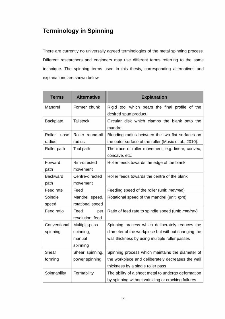
Terminology in Spinning
There are currently no universally agreed terminologies of the metal spinning process.
Different researchers and engineers may use different terms referring to the same
technique. The spinning terms used in this thesis, corresponding alternatives and
explanations are shown below.
Terms Alternative Explanation
Mandrel Former, chunk Rigid tool which bears the final profile of the desired spun product.
Backplate Tailstock Circular disk which clamps the blank onto the mandrel
Roller nose radius
Roller round-off radius
Blending radius between the two flat surfaces on the outer surface of the roller (Music et al., 2010).
Roller path Tool path The trace of roller movement, e.g. linear, convex, concave, etc.
Forward path
Rim-directed movement
Roller feeds towards the edge of the blank
Backward path
Centre-directed movement
Roller feeds towards the centre of the blank
Feed rate Feed Feeding speed of the roller (unit: mm/min)
Spindle speed
Mandrel speed, rotational speed
Rotational speed of the mandrel (unit: rpm)
Feed ratio Feed per revolution, feed
Ratio of feed rate to spindle speed (unit: mm/rev)
Conventional spinning
Multiple-pass spinning, manual spinning
Spinning process which deliberately reduces the diameter of the workpiece but without changing the wall thickness by using multiple roller passes
Shear forming
Shear spinning, power spinning
Spinning process which maintains the diameter of the workpiece and deliberately decreases the wall thickness by a single roller pass
Spinnability Formability The ability of a sheet metal to undergo deformation by spinning without wrinkling or cracking failures
Chapter 1 Introduction
1
1. Introduction
1.1 Background
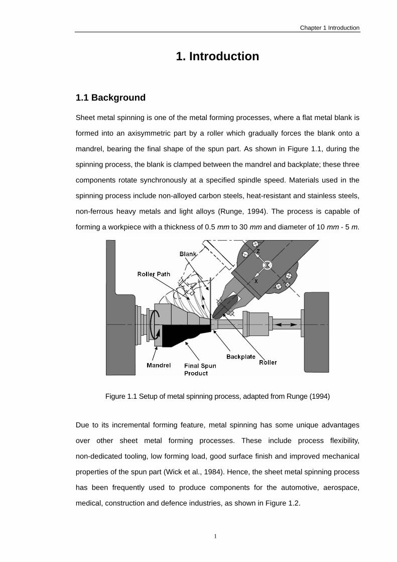
Sheet metal spinning is one of the metal forming processes, where a flat metal blank is
formed into an axisymmetric part by a roller which gradually forces the blank onto a
mandrel, bearing the final shape of the spun part. As shown in Figure 1.1, during the
spinning process, the blank is clamped between the mandrel and backplate; these three
components rotate synchronously at a specified spindle speed. Materials used in the
spinning process include non-alloyed carbon steels, heat-resistant and stainless steels,
non-ferrous heavy metals and light alloys (Runge, 1994). The process is capable of
forming a workpiece with a thickness of 0.5 mm to 30 mm and diameter of 10 mm - 5 m.
Figure 1.1 Setup of metal spinning process, adapted from Runge (1994)
Due to its incremental forming feature, metal spinning has some unique advantages
over other sheet metal forming processes. These include process flexibility,
non-dedicated tooling, low forming load, good surface finish and improved mechanical
properties of the spun part (Wick et al., 1984). Hence, the sheet metal spinning process
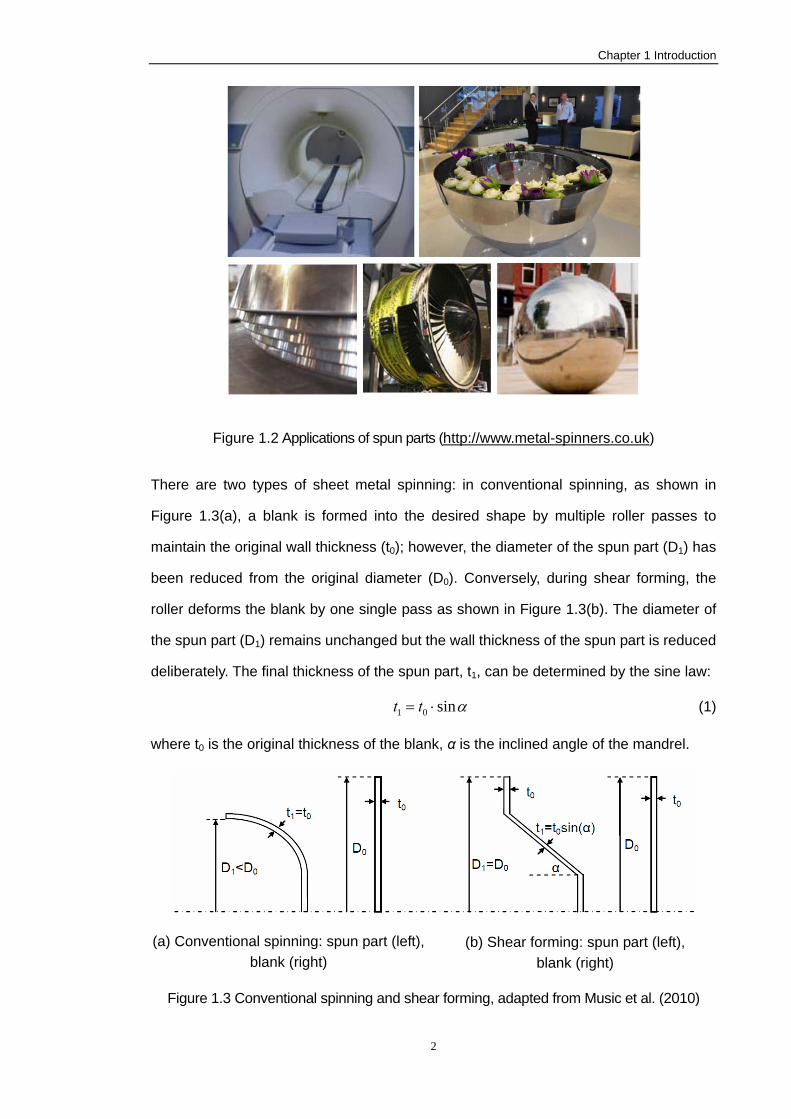
has been frequently used to produce components for the automotive, aerospace,
medical, construction and defence industries, as shown in Figure 1.2.
Chapter 1 Introduction
2
Figure 1.2 Applications of spun parts (http://www.metal-spinners.co.uk)
There are two types of sheet metal spinning: in conventional spinning, as shown in
Figure 1.3(a), a blank is formed into the desired shape by multiple roller passes to
maintain the original wall thickness (t0); however, the diameter of the spun part (D1) has
been reduced from the original diameter (D0). Conversely, during shear forming, the
roller deforms the blank by one single pass as shown in Figure 1.3(b). The diameter of
the spun part (D1) remains unchanged but the wall thickness of the spun part is reduced
deliberately. The final thickness of the spun part, t1, can be determined by the sine law:
αsin01 ⋅= tt (1)
where t0 is the original thickness of the blank, α is the inclined angle of the mandrel.
Figure 1.3 Conventional spinning and shear forming, adapted from Music et al. (2010)
(a) Conventional spinning: spun part (left), blank (right)
(b) Shear forming: spun part (left), blank (right)
Chapter 1 Introduction
3
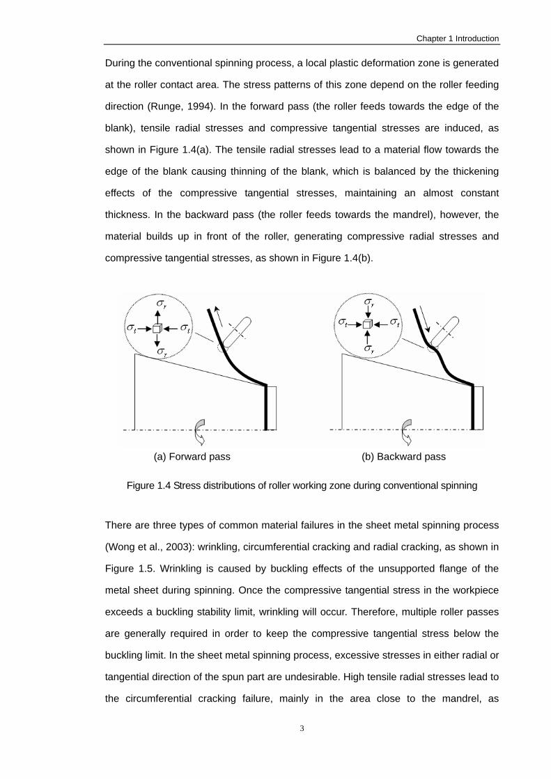
During the conventional spinning process, a local plastic deformation zone is generated
at the roller contact area. The stress patterns of this zone depend on the roller feeding
direction (Runge, 1994). In the forward pass (the roller feeds towards the edge of the
blank), tensile radial stresses and compressive tangential stresses are induced, as
shown in Figure 1.4(a). The tensile radial stresses lead to a material flow towards the
edge of the blank causing thinning of the blank, which is balanced by the thickening
effects of the compressive tangential stresses, maintaining an almost constant
thickness. In the backward pass (the roller feeds towards the mandrel), however, the
material builds up in front of the roller, generating compressive radial stresses and
compressive tangential stresses, as shown in Figure 1.4(b).
(a) Forward pass (b) Backward pass
Figure 1.4 Stress distributions of roller working zone during conventional spinning
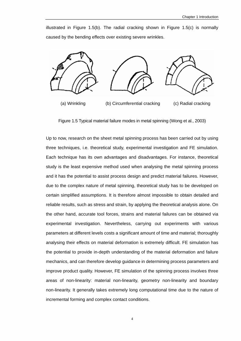
There are three types of common material failures in the sheet metal spinning process
(Wong et al., 2003): wrinkling, circumferential cracking and radial cracking, as shown in
Figure 1.5. Wrinkling is caused by buckling effects of the unsupported flange of the
metal sheet during spinning. Once the compressive tangential stress in the workpiece
exceeds a buckling stability limit, wrinkling will occur. Therefore, multiple roller passes
are generally required in order to keep the compressive tangential stress below the
buckling limit. In the sheet metal spinning process, excessive stresses in either radial or
tangential direction of the spun part are undesirable. High tensile radial stresses lead to
the circumferential cracking failure, mainly in the area close to the mandrel, as
Chapter 1 Introduction
4
illustrated in Figure 1.5(b). The radial cracking shown in Figure 1.5(c) is normally
caused by the bending effects over existing severe wrinkles.
(a) Wrinkling (b) Circumferential cracking (c) Radial cracking
Figure 1.5 Typical material failure modes in metal spinning (Wong et al., 2003)
Up to now, research on the sheet metal spinning process has been carried out by using
three techniques, i.e. theoretical study, experimental investigation and FE simulation.
Each technique has its own advantages and disadvantages. For instance, theoretical
study is the least expensive method used when analysing the metal spinning process
and it has the potential to assist process design and predict material failures. However,
due to the complex nature of metal spinning, theoretical study has to be developed on
certain simplified assumptions. It is therefore almost impossible to obtain detailed and
reliable results, such as stress and strain, by applying the theoretical analysis alone. On
the other hand, accurate tool forces, strains and material failures can be obtained via
experimental investigation. Nevertheless, carrying out experiments with various
parameters at different levels costs a significant amount of time and material; thoroughly
analysing their effects on material deformation is extremely difficult. FE simulation has
the potential to provide in-depth understanding of the material deformation and failure
mechanics, and can therefore develop guidance in determining process parameters and
improve product quality. However, FE simulation of the spinning process involves three
areas of non-linearity: material non-linearity, geometry non-linearity and boundary
non-linearity. It generally takes extremely long computational time due to the nature of
incremental forming and complex contact conditions.
Chapter 1 Introduction
5
The shear forming process has been investigated intensely by many researchers who have
been using both experimental and numerical approaches since 1960. On the other hand,
limited publications on conventional spinning mainly focus on one-pass deep drawing
conventional spinning and simple multi-pass conventional spinning (less than three passes,
linear path profile). The process design of conventional spinning thus still remains a
challenging task and material failures significantly affect production efficiency and
product quality. In the present industrial practice, the trial-and-error approach is commonly
used in the process design (Hagan and Jeswiet, 2003). With the aid of Playback Numerical
Control (PNC) of the spinning machine, all the processing commands developed by
experienced spinners are recorded and used in the subsequent spinning productions
(Pollitt, 1982). Nevertheless, the process design inevitably results in significant variations
and discrepancies in product quality and geometrical dimensions (Hamilton and Long,
2008). Furthermore, the procedure of the PNC process development and validation unduly
wastes a considerable amount of time and materials. It is therefore essential to study the
material deformation and failure mechanics in the multi-pass conventional spinning process
and to analyse the effects of process parameters on the quality of spun products.
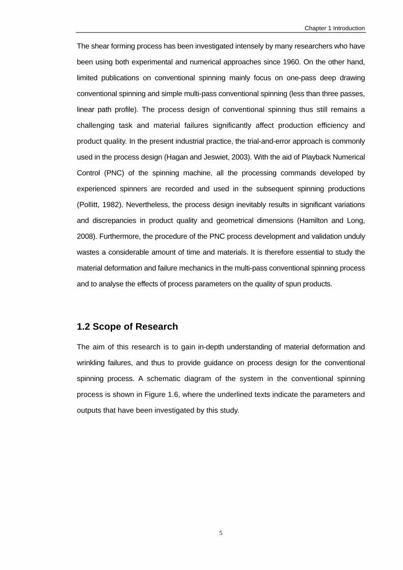
1.2 Scope of Research
The aim of this research is to gain in-depth understanding of material deformation and
wrinkling failures, and thus to provide guidance on process design for the conventional
spinning process. A schematic diagram of the system in the conventional spinning
process is shown in Figure 1.6, where the underlined texts indicate the parameters and
outputs that have been investigated by this study.
Chapter 1 Introduction
6
Figure 1.6 System of conventional spinning process, adapted from Runge (1994)
In this project contributions have been made on six areas of research work on the
conventional spinning process:
1) Finite Element Simulation
3-D elastic-plastic models of metal spinning have been developed using commercial FE
software Abaqus. The explicit FE solution method has been chosen to simulate the
spinning process, because it is more robust and efficient to model 3-D problems that
involve highly nonlinearities. The computing performance of different types of elements
and different scaling methods has been evaluated respectively.
Workpiece Parameters
Blank Thickness
Blank Diameter
Blank Material
Tooling Parameters
Roller Diameter
Roller Nose Radius
Mandrel Diameter
Blank Support Unit
Process Parameters
Feed Rate
Spindle Speed
Feed Ratio
Roller Path (Passes)
Temperature
Lubricant
Outputs
Geometrical Accuracy
Wall Thickness
Tool Forces
Production Time
Stress
Forming Temperature
Hardness
Strain
Surface Finish
Wrinkling Failures
Cracking Failures
Chapter 1 Introduction
7
2) Experimental Investigation
CNC programming has been used to develop roller path (passes) in this study by using
spinning Computer Aided Manufacturing (CAM) software - OPUS. To make the
workpiece successfully conform to the non-linear profile of the mandrel, the tool
compensation techniques have been proposed and employed in the multiple roller
passes design. In addition, the Taguchi method has been used to design an experiment
and to analyse the dimensional variation of spun samples. Experimental investigation
has also been conducted to study the wrinkling failures.
3) Theoretical Analysis of Wrinkling
Energy methods and two-directional plate buckling theory have been used to predict the
critical condition of wrinkling failure in conventional spinning. To predict wrinkling failures,
a theoretical model involving the radial stress, tangential stress, flange dimension and
material property has been developed.
4) Material Deformation
Based on the FE simulation, the variations of tool forces, stresses, strains and wall
thickness have been investigated numerically. Axial force dominates at the beginning of
the conventional spinning; radial force increases gradually over the process; tangential
force is the smallest and remains almost constant. Stress analysis shows that high
tensile and compressive radial stresses take place behind and in front of the roller
contact. Two pairs of oppositely directed radial bending effects have been observed in
the workpiece. The dominated in-plane tensile radial strains of the workpiece are
believed to be the main reason behind the wall thinning.
5) Wrinkling Failures
In order to understand the wrinkling failure mechanics, FE analysis results of tool forces
and stresses of a wrinkle-free model and a wrinkling model have been compared. It is
believed that sudden changes and fluctuations in the tool forces could be used to
determine the approximate moment that wrinkling occurs. If compressive tangential
Chapter 1 Introduction
8
stresses at the flange area near the local forming zone do not fully “recover” to tensile
tangential stresses after leaving roller contact, wrinkling failure will take place.
6) Effects of Parameters
Using a concave roller path produces high tool forces, stresses and reduction of wall
thickness. Conversely, low tool forces, stresses and wall thinning have been obtained in
the FE model which uses the convex roller path. Moreover, results of an experiment
show that the type of material has the most significant effects on the dimensional
variations of spun parts, followed by the effects from feed rate and spindle speed. It has
been shown that high feed ratios help to maintain original blank thickness. However,
high feed ratios also lead to material failures and rough surface finish.
1.3 Structure of Thesis
This thesis consists of seven main chapters, the contents of which are detailed as
below:
Chapter 2 gives a systematic review on the published literature of research on the sheet
metal spinning. Three main investigation techniques used in the research of the sheet
metal spinning process are reviewed, i.e. theoretical study, experimental investigation
and FE analysis. Additionally, research on the material deformation and wrinkling failure
mechanics is presented. Effects of four key process parameters, namely, feed ratio,
roller path (passes), roller profile, and clearance between roller and mandrel, on the
quality of the spun parts are also discussed.
The fundamental theory of Finite Element Method has been discussed in Chapter 3,
such as Hamilton’s Principle and basic analysis procedure of FEM. Moreover, the
formulations of four different types of finite elements, i.e. 3-D solid element, 2-D plane
stress/strain element, plate element and shell element, are presented. Two commonly
used non-linear FE solution methods, implicit method and explicit method, are
compared. Additionally, the elastic-plastic material constitutive model and contact
Chapter 1 Introduction
9
algorithms of FE simulation have been briefly outlined.
Chapter 4 presents an investigation of the effects of roller path profiles on material
deformation. Four roller path profiles are designed and developed to carry out
experimental investigation and FE simulations. The techniques of developing 3-D FE
models of metal spinning are explained in detail. These FE models are verified by
conducting a mesh convergence study, assessing scaling methods and comparing
dimensional results.
In Chapter 5, material deformation in a multi-pass conventional spinning process is
investigated experimentally and numerically. The tool compensation technique is
studied and used in the CNC multiple roller passes design. The Taguchi method is
applied to design the experiment and to analyse the effects of process parameters on
the dimensional variations of spun parts. In addition, FE simulation is conducted to
investigate the variations of tool forces, stresses, wall thickness, and strains in this
multi-pass conventional spinning process.
Theoretical analysis, experimental investigation and FE simulation of the wrinkling
failures in conventional spinning are carried out in Chapter 6. The theory of
two-direction plate buckling and the energy method are employed to determine the
critical condition of wrinkling in the conventional spinning. The severity of wrinkles is
quantified and a forming limit study is carried out by conducting FE simulations.
Furthermore, the computational performance of the solid and shell elements in
simulating the spinning process is examined. Stresses and tool forces are also
investigated in order to gain insight into the wrinkling failure mechanics.
Chapter 7 summarises key conclusions of this study on material deformation and
wrinkling failures in conventional spinning. Future research trends of sheet metal
spinning processes are also outlined.
Chapter 2 Literature Review
10
2. Literature Review
This chapter consists of three main sections which review the published literature of
studies on sheet metal spinning. In Section 2.1, three main investigation techniques in
the research of metal spinning, i.e. theoretical study, experimental investigation and FE
analysis are presented. Section 2.2 outlines research on the material deformation and
wrinkling failure mechanics in the sheet metal spinning process. Section 2.3 discusses
the effects of four key process parameters on the material deformation and failure of the
sheet metal spinning process. The end of this chapter gives a brief summary and
discusses the knowledge gap identified.
2.1 Investigation Techniques
In this section, the methodology of theoretical analysis and experimental investigation
on the tool forces, strains and material failures of the spinning process are reviewed.
Moreover, the key factors in the FE simulation, such as FE solution methods, material
constitutive model, element selection, meshing strategy and contact treatment, are
discussed in detail.
2.1.1 Theoretical Study Compared with the limited theoretical studies on the strain and wrinkling failure, most of
the research work focuses on the theoretical analysis of tool forces, where eight
analytical force models are identified in this literature review. However, all of these
analytical force models are developed for the shear forming but not for conventional
spinning.
2.1.1.1 Analysis of Tool Forces
In those eight published papers, the deformation energy method has been used to
predict the tool forces, i.e. the work done by the external force is assumed to be equal to
Chapter 2 Literature Review
11
the deformation energy of the workpiece. Most of the analytical models developed in
1960s only took the tangential force component into account (Avitzur and Yang, 1960,
Kalpakcioglu, 1961a, Sortais et al., 1963). This is because the tangential force
consumes most of the power in the spinning, and it is thus significantly important for the
design of spinning machines. Researchers (Avitzur and Yang, 1960, Kim et al., 2003,
Kobayashi et al., 1961) calculated the tool force based on the assumption that the
deformation mode in spinning is a combination of bending and shearing. Moreover, by
assuming uniform roller contact pressure, Kobayashi et al. (1961) estimated the radial
and axial forces from the projected contact areas. A similar approach has also been
employed by Chen et al. (2005a), Kim et al. (2006) and Zhang et al. (2010).
2.1.1.2 Prediction of Strains
By assuming hoop strain to be zero in shear forming and neglecting the thickness strain
in conventional spinning on a spherical mandrel, Quigley and Monaghan (2000)
proposed a theoretical analytical method to predict the strains using the constancy of
volume. The verifying experiment indicated that the theoretical strain results only agreed
well in the middle section of workpiece along its radial direction. Beni et al. (2011) also
applied this method and compared the theoretical results with their experimental results.
The authors reported that the theoretical strain models could not predict the strain
values accurately due to unrealistic assumption of zero hoop strain in shear forming and
zero thickness strain in conventional spinning.
2.1.1.3 Investigation of Wrinkling Failures
In general there are two methods to analyse the wrinkling failures of engineering
problems (Senior, 1956): (1) Equilibrium method, where the differential equations for the
system in equilibrium are set up and solved to obtain the critical condition of wrinkling,
such as Euler’s solution for the buckling of a longitudinally loaded column (Gere, 2001).
(2) Energy method, where a deflected form of the part is assumed and the potential
energy related to this small deflection is evaluated. When the total energy which tends
Chapter 2 Literature Review
12
to restore the equilibrium is higher than the energy due to forces displacing it, the
system remains stable (Senior, 1956). The critical condition of wrinkling is given by
equating the two energy values. Until now, very limited theoretical analyses have been
reported on the wrinkling failure of metal spinning processes. Reitmann and Kantz
(2001) used the equilibrium method to analyse various conditions of buckling. They
reported that wrinkling in spinning processes could result from static buckling or
dynamic buckling or both ways. By modifying the instability theory of the deep-drawing
process (Senior, 1956) and using the energy method, Kobayashi (1963) proposed a
theoretical model to determine the critical condition of the flange wrinkling in
conventional spinning on a conical mandrel, with spinning ratio and cone angle as
variables. Nevertheless, this theoretical model was based on an assumption of
neglecting the radial stresses, i.e. one directional beam buckling theory (Chu and Xu,
2001). Therefore, Senior (1956)’s theoretical work may not be accurate in determining
the critical condition of wrinkling failure in metal spinning.
2.1.2 Experimental Investigation
Experimental investigation has been applied to analyse the material deformation and
failure in the sheet metal spinning process since the 1950s. In this literature review, 39
papers of experimental investigation in sheet metal spinning are included. The
methodologies of measuring tool forces, investigating strains and material deformation,
and analysing material failures are presented in this section. The statistical experimental
design methods that have been used in spinning research are also discussed.
2.1.2.1 Measurement of Tool Forces
Experimental investigations into tool forces have been carried out on both shear forming
and conventional spinning. Tool force in the spinning process is normally resolved into
three orthogonal components, e.g. axial force - Fa, radial force - Fr and tangential force -
Ft. However, the definition of force components in the shear forming study is generally
different from that in the conventional spinning study. As shown in Figure 2.1(a), in the
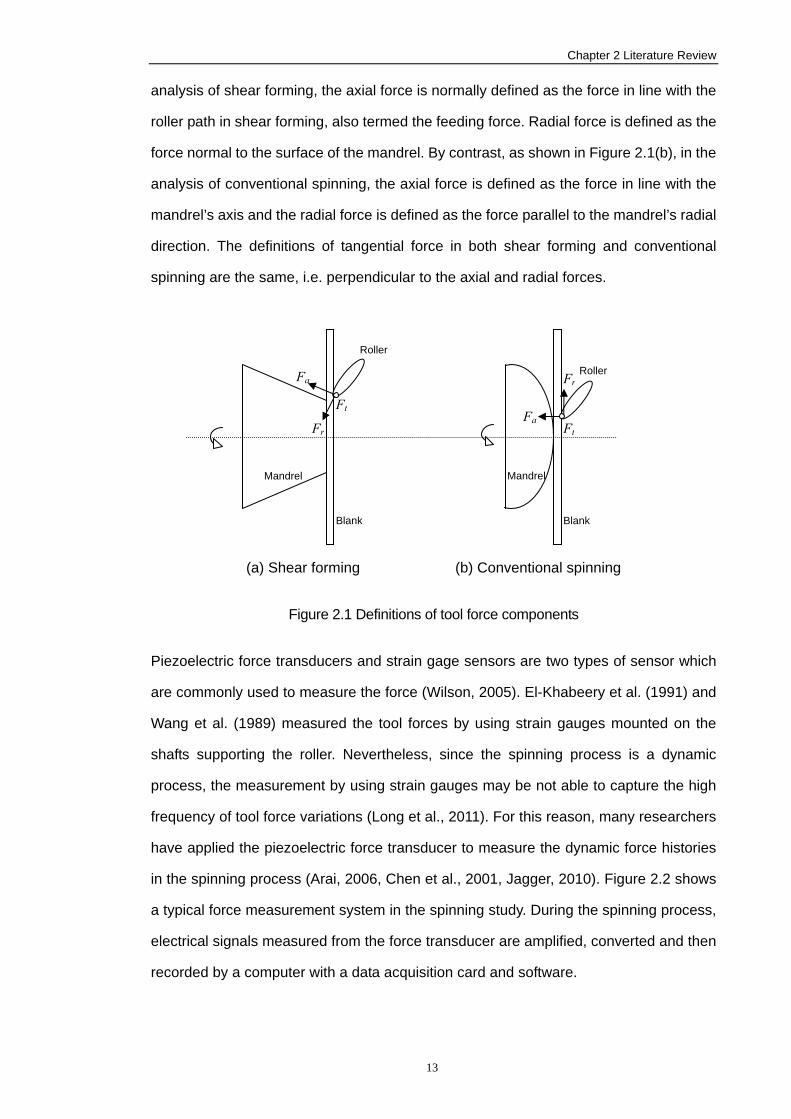
Chapter 2 Literature Review
13
analysis of shear forming, the axial force is normally defined as the force in line with the
roller path in shear forming, also termed the feeding force. Radial force is defined as the
force normal to the surface of the mandrel. By contrast, as shown in Figure 2.1(b), in the
analysis of conventional spinning, the axial force is defined as the force in line with the
mandrel’s axis and the radial force is defined as the force parallel to the mandrel’s radial
direction. The definitions of tangential force in both shear forming and conventional
spinning are the same, i.e. perpendicular to the axial and radial forces.
(a) Shear forming (b) Conventional spinning
Figure 2.1 Definitions of tool force components
Piezoelectric force transducers and strain gage sensors are two types of sensor which
are commonly used to measure the force (Wilson, 2005). El-Khabeery et al. (1991) and
Wang et al. (1989) measured the tool forces by using strain gauges mounted on the
shafts supporting the roller. Nevertheless, since the spinning process is a dynamic
process, the measurement by using strain gauges may be not able to capture the high
frequency of tool force variations (Long et al., 2011). For this reason, many researchers
have applied the piezoelectric force transducer to measure the dynamic force histories
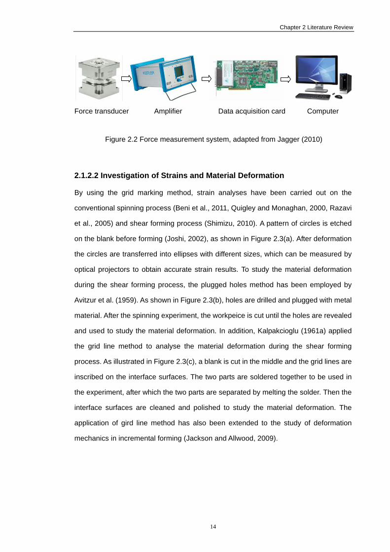
in the spinning process (Arai, 2006, Chen et al., 2001, Jagger, 2010). Figure 2.2 shows
a typical force measurement system in the spinning study. During the spinning process,
electrical signals measured from the force transducer are amplified, converted and then
recorded by a computer with a data acquisition card and software.
Fr
Fa
Ft Fa
Fr
Ft
Mandrel
Blank
Mandrel
Blank
Roller
Roller
Chapter 2 Literature Review
14
Force transducer Amplifier Data acquisition card Computer
Figure 2.2 Force measurement system, adapted from Jagger (2010)
2.1.2.2 Investigation of Strains and Material Deformation
By using the grid marking method, strain analyses have been carried out on the
conventional spinning process (Beni et al., 2011, Quigley and Monaghan, 2000, Razavi
et al., 2005) and shear forming process (Shimizu, 2010). A pattern of circles is etched
on the blank before forming (Joshi, 2002), as shown in Figure 2.3(a). After deformation
the circles are transferred into ellipses with different sizes, which can be measured by
optical projectors to obtain accurate strain results. To study the material deformation
during the shear forming process, the plugged holes method has been employed by
Avitzur et al. (1959). As shown in Figure 2.3(b), holes are drilled and plugged with metal
material. After the spinning experiment, the workpeice is cut until the holes are revealed
and used to study the material deformation. In addition, Kalpakcioglu (1961a) applied
the grid line method to analyse the material deformation during the shear forming
process. As illustrated in Figure 2.3(c), a blank is cut in the middle and the grid lines are
inscribed on the interface surfaces. The two parts are soldered together to be used in
the experiment, after which the two parts are separated by melting the solder. Then the
interface surfaces are cleaned and polished to study the material deformation. The
application of gird line method has also been extended to the study of deformation
mechanics in incremental forming (Jackson and Allwood, 2009).
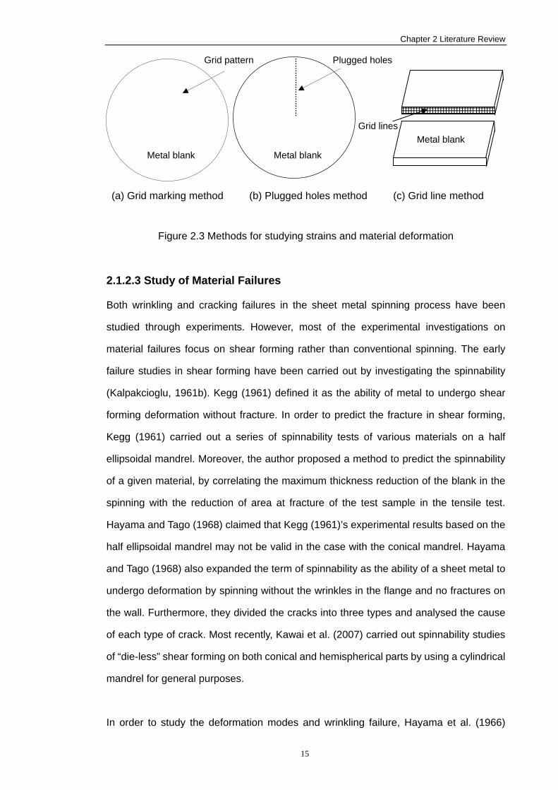
Chapter 2 Literature Review
15
(a) Grid marking method (b) Plugged holes method (c) Grid line method
Figure 2.3 Methods for studying strains and material deformation
2.1.2.3 Study of Material Failures
Both wrinkling and cracking failures in the sheet metal spinning process have been
studied through experiments. However, most of the experimental investigations on
material failures focus on shear forming rather than conventional spinning. The early
failure studies in shear forming have been carried out by investigating the spinnability
(Kalpakcioglu, 1961b). Kegg (1961) defined it as the ability of metal to undergo shear
forming deformation without fracture. In order to predict the fracture in shear forming,
Kegg (1961) carried out a series of spinnability tests of various materials on a half
ellipsoidal mandrel. Moreover, the author proposed a method to predict the spinnability
of a given material, by correlating the maximum thickness reduction of the blank in the
spinning with the reduction of area at fracture of the test sample in the tensile test.
Hayama and Tago (1968) claimed that Kegg (1961)’s experimental results based on the
half ellipsoidal mandrel may not be valid in the case with the conical mandrel. Hayama
and Tago (1968) also expanded the term of spinnability as the ability of a sheet metal to
undergo deformation by spinning without the wrinkles in the flange and no fractures on
the wall. Furthermore, they divided the cracks into three types and analysed the cause
of each type of crack. Most recently, Kawai et al. (2007) carried out spinnability studies
of “die-less” shear forming on both conical and hemispherical parts by using a cylindrical
mandrel for general purposes.
In order to study the deformation modes and wrinkling failure, Hayama et al. (1966)
Metal blank
Grid lines Metal blank
Metal blank
Grid pattern Plugged holes
Chapter 2 Literature Review
16
measured the radial and circumferential strains as well as the periodic variations of
curvatures on the flange, by attaching strain gauges on both sides of the flange before
spinning. In a later study, Hayama (1981) used the sudden change of the vibration of the
axial force (feeding force) to determine the exact moment when the wrinkling occurs in
the shear forming. By applying a laser range sensor to monitor the height of the flange
of the rotating workpiece, Arai (2003) experimentally measured the development of the
wrinkles at different stages of forming. Based on a one-pass deep drawing conventional
spinning experiment, Xia et al. (2005) carried out spinnability studies on blanks made by
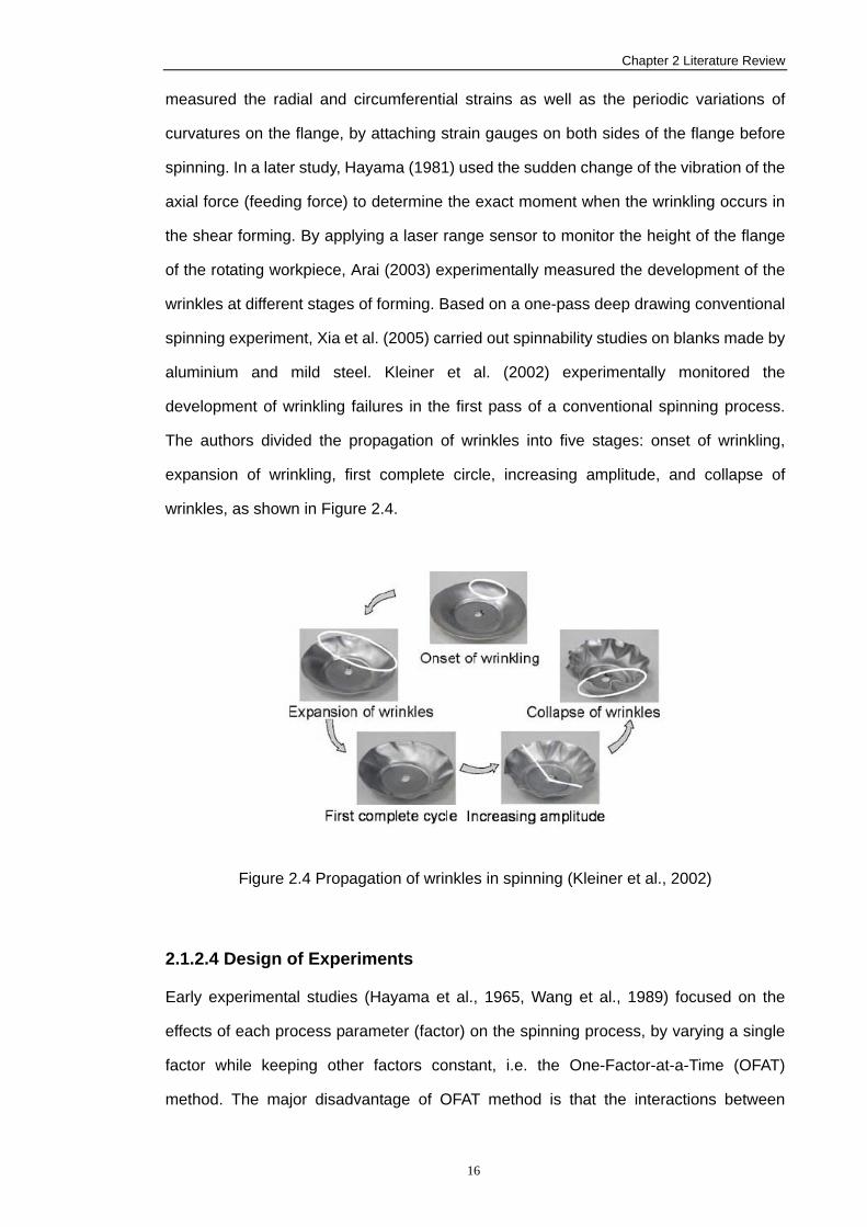
aluminium and mild steel. Kleiner et al. (2002) experimentally monitored the
development of wrinkling failures in the first pass of a conventional spinning process.
The authors divided the propagation of wrinkles into five stages: onset of wrinkling,
expansion of wrinkling, first complete circle, increasing amplitude, and collapse of
wrinkles, as shown in Figure 2.4.
Figure 2.4 Propagation of wrinkles in spinning (Kleiner et al., 2002)
2.1.2.4 Design of Experiments
Early experimental studies (Hayama et al., 1965, Wang et al., 1989) focused on the
effects of each process parameter (factor) on the spinning process, by varying a single
factor while keeping other factors constant, i.e. the One-Factor-at-a-Time (OFAT)
method. The major disadvantage of OFAT method is that the interactions between
Chapter 2 Literature Review
17
different factors cannot be evaluated (Montgomery, 2009). For this reason, Design of
Experiment (DoE) methods, in which several factors are varied simultaneously, have
been employed to analyse the effects of process parameters on the dimensional
variations of spun parts (Auer et al., 2004, Henkenjohann et al., 2005, Kleiner et al.,
2005). Response surface methodology (RSM) has also been applied in the
experimental investigations of tool forces and surface finish (Chen et al., 2001, Chen et
al., 2005b, Jagger, 2010) in the sheet metal spinning process. RSM is a collection of
mathematical and statistical techniques for establishing relations among various
process parameters and optimising the response (Montgomery, 2009). It uses
regression analysis to fit an equation to correlate the response with the process
parameters.
2.1.3 Finite Element Analysis
Since the 1990s, FE analysis of sheet metal spinning process has seen significant
development. In this section, 31 papers on FE analysis of spinning have been reviewed.
Due to the nature of incremental forming, in the early studies, to reduce the computing
time, certain simplifications had to be made. For instance, 2-D FE models (Alberti et al.,
1989, Liu et al., 2002) or simplified 3-D FE models with axisymmetric modeling were
used where the roller was approximated as a virtual ringed tool with variable diameters
(Mori and Nonaka, 2005). More recently, with the development of computing hardware,
3-D FE models have been commonly applied to study the material deformation and
failure mechanics in the spinning process. In this section, five key factors of the FE
simulation are discussed, i.e. the FE solution method, material constitutive model,
element selection, meshing strategy, and contact treatment.
2.1.3.1 Finite Element Solution Methods
Finite Element solution methods are generally resolved into the implicit method and the
explicit method (Harewood and McHugh, 2007). The implicit FE analysis method
iterates to find the approximate static equilibrium at the end of each load increment. It
Chapter 2 Literature Review
18
controls the increment by a convergence criterion throughout the simulation. Because of
the complex contact conditions and high non-linearity in the metal forming problems, a
large number of iterations have to be carried out before finding the equilibrium; the
global stiffness matrix thus has to be assembled and inverted many times during the
analysis. Therefore, the computation is extremely expensive and memory requirements
are also very high (Tekkaya, 2000). Additionally, the implicit method is unable to carry on
the analysis if shape defects, e.g. wrinkling, occur in the sheet metal simulation (Alberti
and Fratini, 2004). It is difficult to predict how long it will take to solve the problem or
even if convergence can be achieved (Harewood and McHugh, 2007). Thus the implicit
method is preferable to analyse some small 2-D problems and 3-D problems under
simple loading conditions, for instance, modelling the springback after spinning (Bai et
al., 2008, Zhan et al., 2008). On the other hand, the explicit FE analysis method
determines a solution by advancing the kinematic state from one time increment to the
next, without iteration. The explicit solution method uses a diagonal mass matrix to
solve for the accelerations and there are no convergence checks. Therefore it is more
robust and efficient for complicated problems, such as dynamic events, nonlinear
behaviors, and complex contact conditions. Hence the explicit FE analysis method has
been chosen by most researchers to analyse the metal spinning process.
2.1.3.2 Material Constitutive Model
The most commonly used yield criterion in engineering application, particularly for
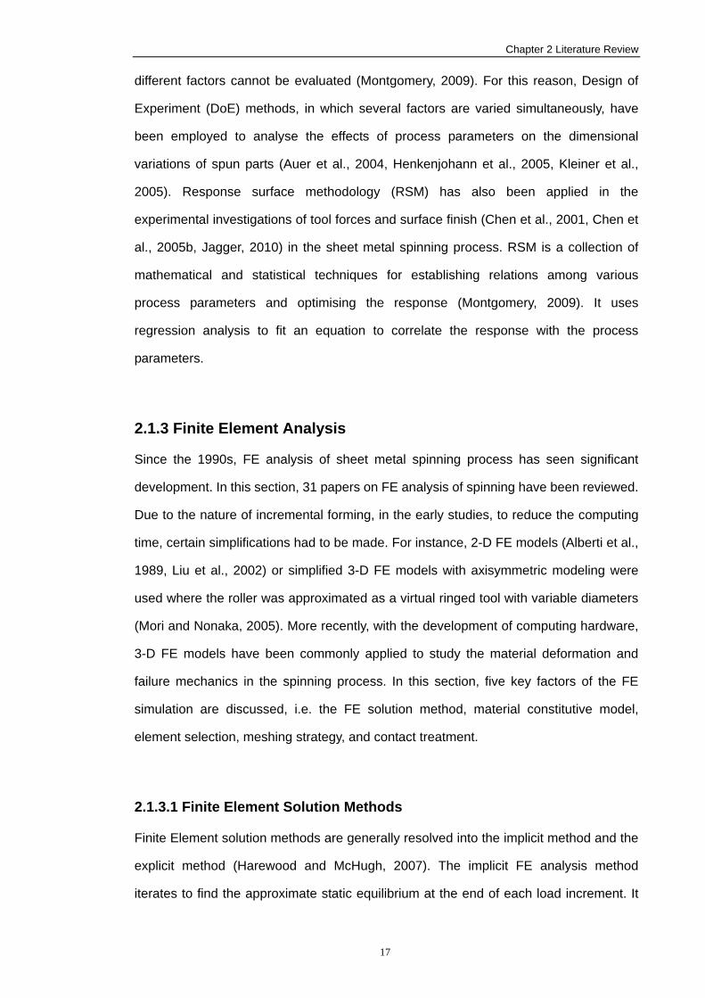
computational analysis, is von Mises criterion (Dunne and Petrinic, 2005). Figure 2.5 (a)
shows the von Mises yield surface of isotropic hardening in 2-D space of principal
stresses (σ1, σ2). In the isotropic material hardening, if the load is reversed at the load
point (1), the material behaves elastically until reaching the load point (2), which is still
on the yield surface. Any stress increase beyond this point will lead to plastic
deformation. Clearly, the isotropic hardening leads to a very large elastic region in the
reversed loading process. However, in reality, a much smaller elastic region is expected
in the reversed loading process. This phenomenon is called the Bauschinger effect
(also known as work softening), i.e. when a metal material is subjected to tension into
Chapter 2 Literature Review
19
the plastic range, after the load is released and compression is applied, the yield stress
in the compression is lower than that in the tension (Kalpakjian and Schmid, 2001).
Kinematic hardening model takes the Bauschinger effect into account, where the yield
surface translates in the stress space rather than expanding, as shown in Figure 2.5(b).
During the spinning process, the roller induces constant tensile and compressive
loadings on the workpiece. Hence, Klimmek et al. (2002) and Pell (2009) suggested that
the Bauschinger effect should not be neglected in the FE simulation of spinning.
However, due to the lack of specific material test data, none of those researchers have
considered the Bauschinger effect.
(a) Isotropic hardening
(b) Kinematic hardening
Figure 2.5 Material hardening models (Dunne and Petrinic, 2005)
Chapter 2 Literature Review
20
2.1.3.3 Element Selection
The accuracy of any FE simulation is highly dependent on the type of element used in
the simulation. Solid elements and shell elements are two types of the most commonly
used elements in metal spinning simulation. Quigley and Monaghan (2002a) suggested
that 8 noded hexahedral solid elements should be used, because a blank modelled by
2-D shell elements may not be able to handle the contact with the roller and mandrel at
the same time. To solve this problem, Zhao et al. (2007) applied an offset of one-half of
the blank thickness from the middle plane to both sides of the 2-D shell element. By
comparing FE results obtained from solid and shell elements, Hamilton and Long (2008)
concluded that wrinkling failure may be exaggerated if using shell elements. Most
recently, Long et al. (2011) reported that the use of continuum shell elements produced
axial force and thickness results which were in good agreement with the experiment.
The FE models using solid elements produced considerably different tool force results
in comparison with the experimentally measured axial and radial force values.
During the metal spinning process, the material undergoes a complicated loading
process that includes bending effects (Sebastiani et al., 2007), which may cause the
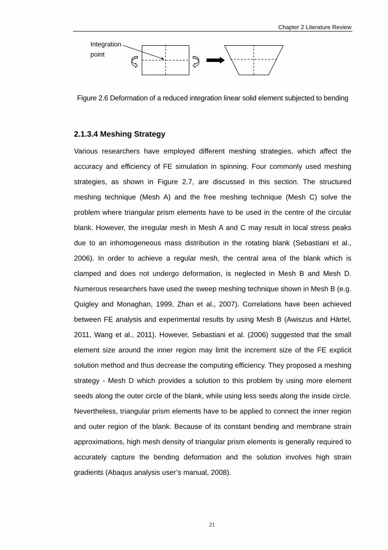
“hourglassing” problem as a result of using reduced integration linear solid elements. As
shown in Figure 2.6, the bending of a reduced integration linear solid element presents
a zero-energy deformation mode, as no strain energy is generated by the element
distortion (Abaqus analysis user’s manual, 2008). Moreover, this “hourglassing”
problem can propagate through the elements and produce meaningless numerical
results. On the other hand, unlike the reduced integration linear solid element, which
only uses one integration point along the thickness direction, multiple integration points
are used through the thickness of a reduced integration linear shell element. Stresses
and strains at each integration point of the shell element are calculated independently.
This may be the reason why reduced integration linear shell elements can produce
more accurate results of wrinkling (Wang et al., 2011) and tool forces (Long et al., 2011)
than reduced integration linear solid elements.
Chapter 2 Literature Review
21
Figure 2.6 Deformation of a reduced integration linear solid element subjected to bending
2.1.3.4 Meshing Strategy
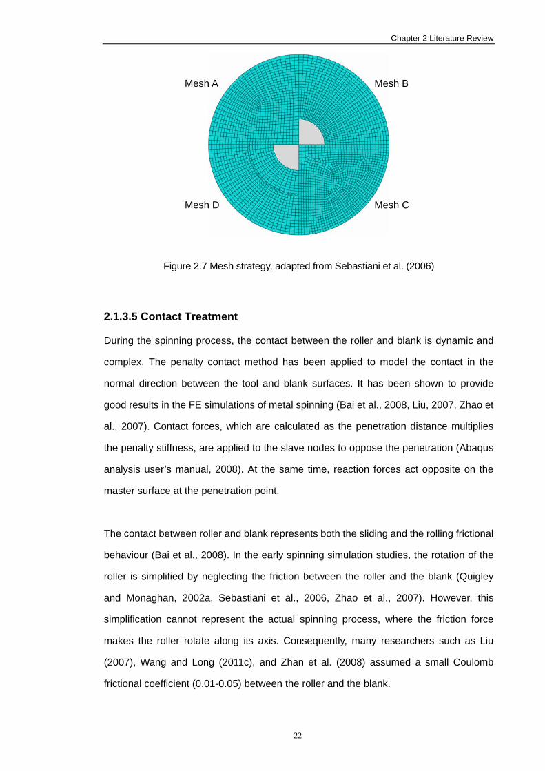
Various researchers have employed different meshing strategies, which affect the
accuracy and efficiency of FE simulation in spinning. Four commonly used meshing
strategies, as shown in Figure 2.7, are discussed in this section. The structured
meshing technique (Mesh A) and the free meshing technique (Mesh C) solve the
problem where triangular prism elements have to be used in the centre of the circular
blank. However, the irregular mesh in Mesh A and C may result in local stress peaks
due to an inhomogeneous mass distribution in the rotating blank (Sebastiani et al.,
2006). In order to achieve a regular mesh, the central area of the blank which is
clamped and does not undergo deformation, is neglected in Mesh B and Mesh D.
Numerous researchers have used the sweep meshing technique shown in Mesh B (e.g.
Quigley and Monaghan, 1999, Zhan et al., 2007). Correlations have been achieved
between FE analysis and experimental results by using Mesh B (Awiszus and Härtel,
2011, Wang et al., 2011). However, Sebastiani et al. (2006) suggested that the small
element size around the inner region may limit the increment size of the FE explicit
solution method and thus decrease the computing efficiency. They proposed a meshing
strategy - Mesh D which provides a solution to this problem by using more element
seeds along the outer circle of the blank, while using less seeds along the inside circle.
Nevertheless, triangular prism elements have to be applied to connect the inner region
and outer region of the blank. Because of its constant bending and membrane strain
approximations, high mesh density of triangular prism elements is generally required to
accurately capture the bending deformation and the solution involves high strain
gradients (Abaqus analysis user’s manual, 2008).
Integration point
Chapter 2 Literature Review
22
Figure 2.7 Mesh strategy, adapted from Sebastiani et al. (2006)
2.1.3.5 Contact Treatment
During the spinning process, the contact between the roller and blank is dynamic and
complex. The penalty contact method has been applied to model the contact in the
normal direction between the tool and blank surfaces. It has been shown to provide
good results in the FE simulations of metal spinning (Bai et al., 2008, Liu, 2007, Zhao et
al., 2007). Contact forces, which are calculated as the penetration distance multiplies
the penalty stiffness, are applied to the slave nodes to oppose the penetration (Abaqus
analysis user’s manual, 2008). At the same time, reaction forces act opposite on the
master surface at the penetration point.
The contact between roller and blank represents both the sliding and the rolling frictional
behaviour (Bai et al., 2008). In the early spinning simulation studies, the rotation of the
roller is simplified by neglecting the friction between the roller and the blank (Quigley
and Monaghan, 2002a, Sebastiani et al., 2006, Zhao et al., 2007). However, this
simplification cannot represent the actual spinning process, where the friction force
makes the roller rotate along its axis. Consequently, many researchers such as Liu
(2007), Wang and Long (2011c), and Zhan et al. (2008) assumed a small Coulomb
frictional coefficient (0.01-0.05) between the roller and the blank.
Mesh A Mesh B
Mesh C Mesh D
Chapter 2 Literature Review
23
2.2 Material Deformation and Wrinkling Failure
In this section, published literature regarding the tool forces, stresses and strains, and
wrinkling failures in both shear forming process and conventional spinning process are
reviewed. Analysing tool forces in the sheet metal spinning process is important to
select process parameters, design spinning machines, and improve the quality of spun
products (Wang et al., 1989). Moreover, investigating stresses, strains and material
failures is essential to understand the deformation and failure mechanics and thus
optimise the process design.
2.2.1 Tool forces
Until now, tool forces in shear forming, one-pass deep drawing conventional spinning,
and multi-pass conventional spinning processes have been investigated intensively.
Among the three force components generated in shear forming, as defined in Figure
2.1(a), the radial force is the highest, because the roller squeezes the material onto the
mandrel during the whole process. The axial force ranks the second and the tangential
force is the smallest (Arai, 2003, Hayama et al., 1965, Zhan et al., 2007). As reported in
an experimental investigation of shear forming (Lee and Noble, 1982), both axial force
and radial force decrease when increasing the angle between the roller axis and
mandrel axis from 0°to approximately 60°with a slight increase thereafter. The tool
forces would also decrease if a thinner blank were used (Chen et al., 2001, Hayama et
al., 1965).
According to the experimental investigations of one-pass deep drawing conventional
spinning (Hayama and Murota, 1963, Jurkovic et al., 2006, Xia et al., 2005), the peak
values of the axial force are obtained at the middle stage of spinning. On the other hand,
the maximum values of the radial force occur at the end of the process. The tangential
force is again the smallest force among these three force components and it remains
almost constant during the one-pass deep drawing spinning process.
Tool forces of the multi-pass conventional spinning process have been experimentally
Chapter 2 Literature Review
24
investigated (Jagger, 2010, Wang et al., 1989) and analysed by FE simulation (Essa
and Hartley, 2009, Liu, 2007, Pell, 2009). It has been reported that in the conventional
spinning process, among three force components as defined in Figure 2.1(b), the axial
force is the largest, while the tangential force is the lowest. In a 3-pass conventional
spinning experiment, Wang et al. (1989) reported that when the thickness of the blank
increases, tool forces increase accordingly. Wang et al. (1989) also gave an
approximately proportional relationship among the peak values of the force components,
where
Fa : Fr : Ft = 20 : 10 : 1 (2)
The maximum force ratios obtained in an experiment (Jagger, 2010) and FE simulation
(Wang and Long, 2011b) of 3-pass conventional spinning processes show a similar
trend, as illustrated in equation (3) and (4), respectively.
Fa : Fr : Ft = 17 : 5 : 1 (3)
Fa : Fr : Ft = 35 : 17 : 1 (4)
Recently, Wang and Long (2011a) numerically compared the force histories when the
workpieces were made of three material types in a multi-pass conventional spinning
process. The authors reported that a FE model using stainless steel produced the
highest tool forces, followed by a model using mild steel, while the lowest tool forces
were obtained in a model using aluminium. Wang and Long (2011a) also compared the
maximum tool forces of a wrinkle-free model and a wrinkling model; the tool forces in
the wrinkle-free models were approximately one third of the corresponding forces in the
wrinkling models.
2.2.2 Stresses
Klimmek et al. (2002) suggested that investigating the stress distribution of the
workpiece, especially within the local forming zone, is essential to understand the cause
of the wrinkling failure. The authors investigated the stress variations of two distinct
elements during a forward roller pass. The first element is close to the centre of the
blank, while the second element is located at the rim of the blank. They reported that
Chapter 2 Literature Review
25
once the first element gets into the local forming zone, the tensile radial stress steadily
increases to a maximum value. By contrast, as the roller gets to the edge of the blank,
the compressive tangential stress of the second element increases dramatically.
Sebastiani et al. (2007) developed a spinning model which uses three linear roller
passes, including both forward passes and backward passes. The authors report that
local radial bending effects exist in the workpiece during a forward pass, where the inner
surface (mandrel facing) of the workpiece is subjected to compressive radial stresses
while its outer surface (roller facing) is under tensile radial stresses, as also observed by
Pell (2009) and Wang and Long (2010). Moreover, after a backward roller pass, a
toothed stress pattern in the flange region has been observed by Sebastiani et al.
(2007), who believe that it may be the pre-state of the wrinkling failure. A similar toothed
stress pattern has also been noticed during a non-linear backward pass by Wang and
Long (2011b). However, no correlations have been found between the toothed stress
pattern and wrinkling failure.
2.2.3 Strains
Theoretically, in the conventional spinning process, the compressive hoop strain should
balance the tensile radial strain. The thickness strain thus remains zero. However, in an
experimental investigation of a one-pass deep drawing conventional spinning process
(Hayama and Murota, 1963), tensile radial and hoop strains resulting in compressive
thickness strains, have been observed at the bottom of a spun part. However, in the
opening of a spun part, the unbalanced compressive hoop strains and tensile radial
strains lead to a certain amount of tensile thickness strains. Thinning at the bottom and
thickening in the opening of the spun parts in one-pass deep drawing conventional
spinning have also been reported by Hamilton and Long (2008) and Xia et al. (2005).
The experimental results of the multi-pass conventional spinning on the spherical
mandrel (Beni et al., 2011, Quigley and Monaghan, 2000, Razavi et al., 2005) show that
the tensile radial strain and compressive hoop strain do not mirror each other, thus
indicating that a certain amount of thickness strain exists in the workpiece, as confirmed
Chapter 2 Literature Review
26
in the FE simulations by Wang and Long (2011b). In addition, Quigley and Monaghan
(2000) reported that there was a certain degree of shear forming involved in the first
roller pass of conventional spinning.
In the shear forming process, considerably high tensile radial strain and compressive
thickness strain have been observed by Shimizu (2010), who experimentally
investigated the strain distributions along the radial direction of the workpiece. By
contrast, tangential strain keeps almost constant, only a slightly increase is observed in
the opening of the spun part. Bending strains have been measured by strain gauges
that mounted on both sides of the workpiece (Hayama et al., 1966), where bending and
unbending are performed repeatedly in the local forming zone of the shear forming.
2.2.4 Wrinkling Failure
It is believed that in sheet metal spinning wrinkling takes place when the tangential
compressive stress in the flange exceeds the buckling stability limit (Kleiner et al., 2002,
Klimmek et al., 2002, Runge, 1994). However, it is still unknown how to determine the
buckling limit which could be used to predict and prevent wrinkling failure. Kleiner et al.
(2002) suggested that the wrinkling in the spinning process is not only caused by static
buckling, but also influenced or even triggered by the dynamic effects from the feeding
of roller and rotation of the workpiece.
The experimental results of Kleiner et al. (2002) indicate that the diameter and thickness
have the most significant effects on wrinkling failure, followed by the feed rate, the
spindle speed, the roller path and the material of the workpiece. Hayama et al. (1966)
also reported that the feed ratio, blank thickness and blank diameter are very important
contributing factors to wrinkling failure. Hayama (1981) suggested that the feed ratio is
the most important parameter affecting spinnability. In general, wrinkles tend to occur
when increasing the feed ratio and blank diameter or decreasing the blank thickness
(Hayama et al., 1966, Kleiner et al., 2002, Xia et al., 2005).
Chapter 2 Literature Review
27
Satoh and Yanagimoto (1982) reported that wrinkling resistance would be enhanced if a
material with higher yielding stress was used, as they believe wrinkling occurs due to
elastic buckling. Wang and Long (2011a) proposed that there may be a limit to the roller
feed depth, beyond which wrinkling failures may take place. Furthermore, both Kawai
and Hayama (1987) and Wang et al. (2011) reported that wrinkles may be smoothed out
in subsequent passes of conventional spinning processes. Although several
investigations have been conducted on the wrinkling failure of metal spinning, further
investigation is still required to gain an in-depth understanding of wrinkling failure
mechanics, the effects of process parameters, and to predict and prevent wrinkling
failures.
2.3 Key Process Parameters
The process parameters play a decisive role in the design and optimisation of sheet
metal spinning process. The effects of four key process parameters, i.e. feed ratio, roller
path (passes), roller profile, and clearance between roller and mandrel, on the material
deformation and failures of the spun parts are discussed in this section.
2.3.1 Feed Ratio
Feed ratio is defined as the ratio of the roller feed rate to the spindle speed. As long as
the feed ratio remains constant, by changing the feed rate and the spindle speed
proportionally, there would be no significant effects on the tool forces (Hayama et al.,
1965, Jagger, 2010, Lee and Noble, 1982, Wang et al., 2011, Wang et al., 1989, Xia et
al., 2005), wall thickness (Xia et al., 2005, Zhan et al., 2008), wrinkling failures (Hayama
et al., 1966, Wang et al., 2011), cracking failures (Hayama and Tago, 1968) and surface
finish (Ma et al., 2010) of the spun part.
Nevertheless, it has been reported that variation of feed ratio has considerable effects
on the tool force, wall thickness, spinnability, surface finish and springback of the metal
spinning process. When a higher feed ratio is applied, tool forces will increase
Chapter 2 Literature Review
28
accordingly (El-Khabeery et al., 1991, Essa and Hartley, 2009, Hayama et al., 1965,
Jagger, 2010, Liu, 2007, Ozer and Arai, 2009, Pell, 2009, Perez et al., 1984, Xia et al.,
2005, Zhan et al., 2007). In addition, material failures tend to take place if a high feed
ratio is used (Hayama, 1981, Hayama et al., 1966, Kawai et al., 2007, Ozer and Arai,
2009, Wang et al., 2011, Xia et al., 2005, Zhan et al., 2007).
On the other hand, Wong et al. (2003) suggested that a low feed ratio would result in
excessive material flow in the outward direction, which unduly thins the blank, as Pell
(2009), Wang et al. (2011) and Zhan et al. (2007) also reported. However, a lower feed
ratio would result in a better surface finish of the spun part (Chen et al., 2001,
El-Khabeery et al., 1991, Kleiner et al., 2005, Ma et al., 2010, Slater, 1979a, Wang et al.,
2011, Slater, 1979a). Both El-Khabeery et al. (1991) and Essa and Hartley (2010)
reported that springback would increase when a higher feed ratio is used.
2.3.2 Roller Path and Passes
By using multiple roller passes in conventional spinning, the tensile radial and
compressive tangential stresses are induced gradually; hence material failures can be
prevented (Runge, 1994, Sebastiani et al., 2007). Up to now, most investigations of
roller path and passes in conventional spinning have focused on single pass or
multi-pass with no more than 3 passes (mainly linear path). Consequently, there is still a
huge knowledge gap between academic research and industrial production, where a
considerable amount of roller passes have to be used to successfully produce
complicated spinning parts (Filip and Neago, 2010). Three types of the roller path
shown in Figure 2.8, straight line, concave curve and convex curve, have been
experimentally studied by Kang et al. (1999) and Hayama et al. (1970). The difference
between these two experiments was that only the single pass was studied by Kang et al.;
whereas multiple passes were investigated by Hayama et al. Kang et al. (1999)
concluded that the first pass in the conventional spinning plays a decisive role in the
final blank thickness. After comparing four different types of roller path designs, Hayama
et al. (1970) proposed that the involute curve path, which is a special type of concave
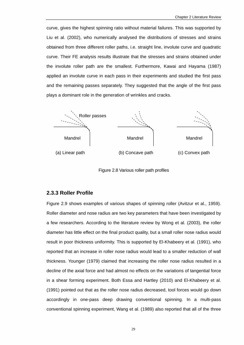
Chapter 2 Literature Review
29
curve, gives the highest spinning ratio without material failures. This was supported by
Liu et al. (2002), who numerically analysed the distributions of stresses and strains
obtained from three different roller paths, i.e. straight line, involute curve and quadratic
curve. Their FE analysis results illustrate that the stresses and strains obtained under
the involute roller path are the smallest. Furthermore, Kawai and Hayama (1987)
applied an involute curve in each pass in their experiments and studied the first pass
and the remaining passes separately. They suggested that the angle of the first pass
plays a dominant role in the generation of wrinkles and cracks.
(a) Linear path (b) Concave path (c) Convex path
Figure 2.8 Various roller path profiles
2.3.3 Roller Profile
Figure 2.9 shows examples of various shapes of spinning roller (Avitzur et al., 1959).
Roller diameter and nose radius are two key parameters that have been investigated by
a few researchers. According to the literature review by Wong et al. (2003), the roller
diameter has little effect on the final product quality, but a small roller nose radius would
result in poor thickness uniformity. This is supported by El-Khabeery et al. (1991), who
reported that an increase in roller nose radius would lead to a smaller reduction of wall
thickness. Younger (1979) claimed that increasing the roller nose radius resulted in a
decline of the axial force and had almost no effects on the variations of tangential force
in a shear forming experiment. Both Essa and Hartley (2010) and El-Khabeery et al.
(1991) pointed out that as the roller nose radius decreased, tool forces would go down
accordingly in one-pass deep drawing conventional spinning. In a multi-pass
conventional spinning experiment, Wang et al. (1989) also reported that all of the three
Mandrel Mandrel Mandrel
Roller passes
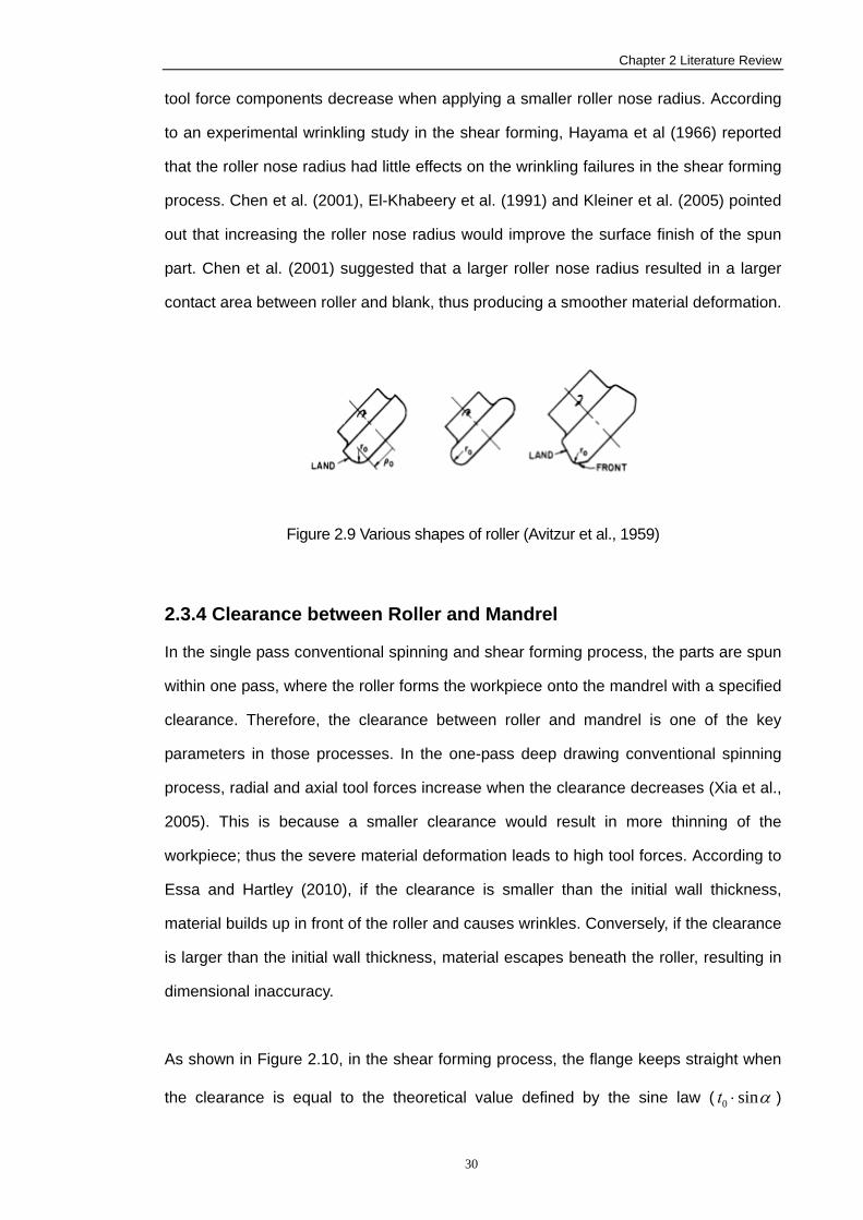
Chapter 2 Literature Review
30
tool force components decrease when applying a smaller roller nose radius. According
to an experimental wrinkling study in the shear forming, Hayama et al (1966) reported
that the roller nose radius had little effects on the wrinkling failures in the shear forming
process. Chen et al. (2001), El-Khabeery et al. (1991) and Kleiner et al. (2005) pointed
out that increasing the roller nose radius would improve the surface finish of the spun
part. Chen et al. (2001) suggested that a larger roller nose radius resulted in a larger
contact area between roller and blank, thus producing a smoother material deformation.
Figure 2.9 Various shapes of roller (Avitzur et al., 1959)
2.3.4 Clearance between Roller and Mandrel
In the single pass conventional spinning and shear forming process, the parts are spun
within one pass, where the roller forms the workpiece onto the mandrel with a specified
clearance. Therefore, the clearance between roller and mandrel is one of the key
parameters in those processes. In the one-pass deep drawing conventional spinning
process, radial and axial tool forces increase when the clearance decreases (Xia et al.,
2005). This is because a smaller clearance would result in more thinning of the
workpiece; thus the severe material deformation leads to high tool forces. According to
Essa and Hartley (2010), if the clearance is smaller than the initial wall thickness,
material builds up in front of the roller and causes wrinkles. Conversely, if the clearance
is larger than the initial wall thickness, material escapes beneath the roller, resulting in
dimensional inaccuracy.
As shown in Figure 2.10, in the shear forming process, the flange keeps straight when
the clearance is equal to the theoretical value defined by the sine law ( αsin0 ⋅t )
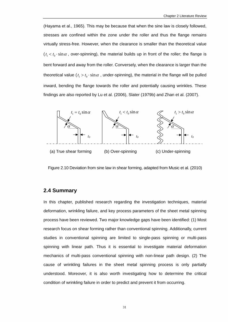
Chapter 2 Literature Review
31
(Hayama et al., 1965). This may be because that when the sine law is closely followed,
stresses are confined within the zone under the roller and thus the flange remains
virtually stress-free. However, when the clearance is smaller than the theoretical value
( αsin01 ⋅< tt , over-spinning), the material builds up in front of the roller; the flange is
bent forward and away from the roller. Conversely, when the clearance is larger than the
theoretical value ( αsin01 ⋅> tt , under-spinning), the material in the flange will be pulled
inward, bending the flange towards the roller and potentially causing wrinkles. These
findings are also reported by Lu et al. (2006), Slater (1979b) and Zhan et al. (2007).
(a) True shear forming (b) Over-spinning (c) Under-spinning
Figure 2.10 Deviation from sine law in shear forming, adapted from Music et al. (2010)
2.4 Summary
In this chapter, published research regarding the investigation techniques, material
deformation, wrinkling failure, and key process parameters of the sheet metal spinning
process have been reviewed. Two major knowledge gaps have been identified: (1) Most
research focus on shear forming rather than conventional spinning. Additionally, current
studies in conventional spinning are limited to single-pass spinning or multi-pass
spinning with linear path. Thus it is essential to investigate material deformation
mechanics of multi-pass conventional spinning with non-linear path design. (2) The
cause of wrinkling failures in the sheet metal spinning process is only partially
understood. Moreover, it is also worth investigating how to determine the critical
condition of wrinkling failure in order to predict and prevent it from occurring.
t0
αsin01 tt = αsin01 tt < αsin01 tt >
t0 t0
α α α
Chapter 3 Fundamentals of Finite Element Method
32
3. Fundamentals of Finite Element Method
The Finite Element Method (FEM) is a numerical method seeking an approximated
solution of a complex engineering problem which is difficult to obtain analytically. It is
realised by dividing the complicated analysis body into a finite number of elements. The
behaviour of each element, which is in regular shape, may be predicted by certain
mathematical equations. The summation of the individual element behaviours produces
the expected behaviour of the whole analysis body. FEM was originally developed for
solving complex elasticity and structural analysis problems in civil and aeronautical
engineering in 1940s. By the early 70s, applications of FEM were limited in aeronautics,
automotive, defence and nuclear industries, executed on expensive mainframe
computers. Over the past decades, due to the rapid developing of computing capability,
FEM has been widely used for analysing the problems involving solid mechanics, fluid
mechanics, heat transfer, vibrations, electrical and magnetic fields, etc. The most
common applications of FEM in industry are to design new products and processes,
optimise existing products and processes so as to improve their performance. In this
chapter, the fundamentals of Finite Element method, such as, Hamilton’s Principle, the
basic analysis procedure of FEM, and four types of finite elements are discussed in
detail. Furthermore, the non-linear solution method, material constitutive model and
contact algorithm are briefly outlined.
3.1 Hamilton’s Principle
To obtain a solution of any solid mechanics FE problems, it is essential to satisfy the
requirements of equilibrium, compatibility, constitutive equations and boundary
conditions. However, obtaining the exact solution (known as strong form) of the
equilibrium is usually extremely difficult for practical engineering problems. Instead, a
weak form of equilibrium for the body as a whole is imposed even though it does not
ensure pointwise equilibrium (Dunne and Petrinic, 2005). Hamilton’s Principal, resulting
from the Conservation of Energy, is one of the most commonly used weak form of
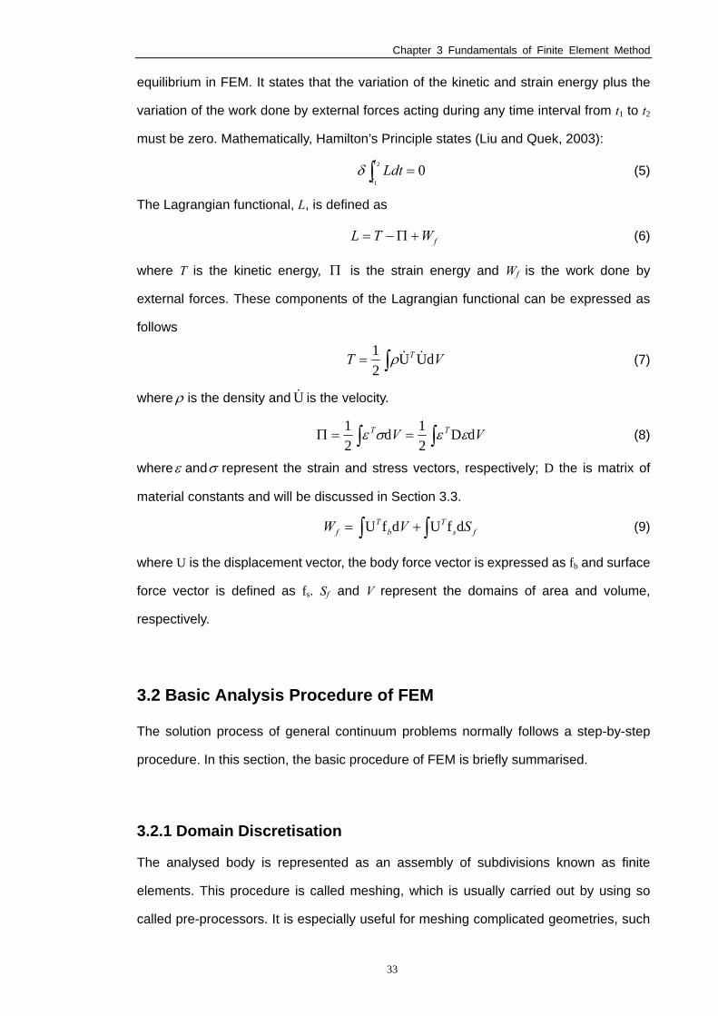
Chapter 3 Fundamentals of Finite Element Method
33
equilibrium in FEM. It states that the variation of the kinetic and strain energy plus the
variation of the work done by external forces acting during any time interval from t1 to t2
must be zero. Mathematically, Hamilton’s Principle states (Liu and Quek, 2003):
∫ =2
1
0t
tLdtδ (5)
The Lagrangian functional, L, is defined as
fWTL +Π−= (6)
where T is the kinetic energy, Π is the strain energy and Wf is the work done by
external forces. These components of the Lagrangian functional can be expressed as
follows
∫= VT T dUU21 &&ρ (7)
where ρ is the density and U& is the velocity.
∫∫ ==Π VV TT dD21d
21 εεσε (8)
whereε andσ represent the strain and stress vectors, respectively; D the is matrix of
material constants and will be discussed in Section 3.3.
∫∫ += fsT
bT
f SVW dfUdfU (9)
where U is the displacement vector, the body force vector is expressed as fb and surface
force vector is defined as fs. Sf and V represent the domains of area and volume,
respectively.
3.2 Basic Analysis Procedure of FEM
The solution process of general continuum problems normally follows a step-by-step
procedure. In this section, the basic procedure of FEM is briefly summarised.
3.2.1 Domain Discretisation
The analysed body is represented as an assembly of subdivisions known as finite
elements. This procedure is called meshing, which is usually carried out by using so
called pre-processors. It is especially useful for meshing complicated geometries, such
Chapter 3 Fundamentals of Finite Element Method
34
as the example shown in Figure 3.1, where a cargo train body is meshed with
thousands of finite elements. The elements are considered to be interconnected at
specified joints called nodes. The selection of the type, number and size of finite
elements are decided based on the characteristic of the analysed problem.
Figure 3.1 Finite Element Meshing (Wang, 2005)
3.2.2 Displacement Interpolation
Because the displacement solution in a complex structure under specified loading
conditions cannot be predicted exactly, in FEM the displacement within an element is
simply assumed by polynomial interpolation using the displacements at its nodes (Liu
and Quek, 2003):
∑=
==dn
ieii zyxzyxzyx
1
d),,(Nd),,(N),,(U (10)
where nd is the number of nodes forming the element; di is the nodal displacement at the
i th node and can be expressed in a general form of
Chapter 3 Fundamentals of Finite Element Method
35
⎪⎪⎭
⎪⎪⎬
⎫
⎪⎪⎩
⎪⎪⎨
⎧
=
fn
i
d
dd
M2
1
d (11)
where nf is the number of Degree Of Freedom (DOF) at a node.
The vector de in equation (10) represents the displacement vector of the entire element
and it has the form of
⎪⎪⎭
⎪⎪⎬
⎫
⎪⎪⎩
⎪⎪⎨
⎧
=
dnd
dd
d 2
1
e M (12)
Thus the total DOF of the entire element is nd × nf.
In equation (10), N is the matrix defining shape functions for the nodes in an element. It
is predefined to assume the variations of displacement with respect to the coordinates
of the element.
]),,(N...),,(N),,(N[),,(N 21 zyxzyxzyxzyxdn= (13)
where Ni is a sub-matrix of the shape functions for displacement components, which is
arranged as
⎥⎥⎥⎥⎥
⎦
⎤
⎢⎢⎢⎢⎢
⎣
⎡
=
fin
i
i
i
N
NN
000000000000
N 2
1
O (14)
where Nik is the shape function for the kth displacement component (DOF) at the i th
node.
3.2.3 Construction of Shape Function For an element with nd nodes at space coordinates xi (i = 1, 2,....,nd), where xT = {x} for
one-dimensional problems, xT = {x, y} for 2-D problems, and xT = {x, y, z} for 3-D
problems, its displacement component u is approximated as (Liu and Quek, 2003)
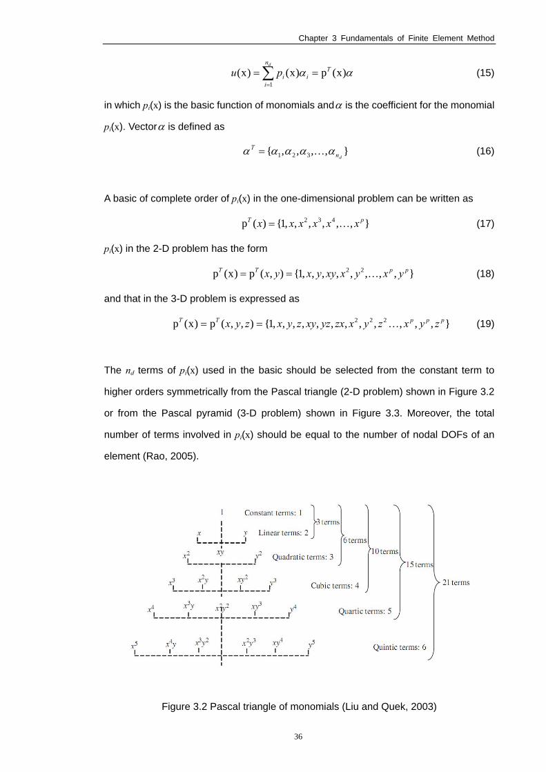
Chapter 3 Fundamentals of Finite Element Method
36
αα )x(p)x()x(1
Tn
iii
d
pu == ∑=
(15)
in which pi(x) is the basic function of monomials andα is the coefficient for the monomial
pi(x). Vectorα is defined as
},,,,{ 321 dnT ααααα K= (16)
A basic of complete order of pi(x) in the one-dimensional problem can be written as
},,,,,,1{)(p 432 pT xxxxxx K= (17)
pi(x) in the 2-D problem has the form
},,,,,,,,1{),(p)x(p 22 ppTT yxyxxyyxyx K== (18)
and that in the 3-D problem is expressed as
},,,,,,,,,,,,1{),,(p)x(p 222 pppTT zyxzyxzxyzxyzyxzyx K== (19)
The nd terms of pi(x) used in the basic should be selected from the constant term to
higher orders symmetrically from the Pascal triangle (2-D problem) shown in Figure 3.2
or from the Pascal pyramid (3-D problem) shown in Figure 3.3. Moreover, the total
number of terms involved in pi(x) should be equal to the number of nodal DOFs of an
element (Rao, 2005).
Figure 3.2 Pascal triangle of monomials (Liu and Quek, 2003)
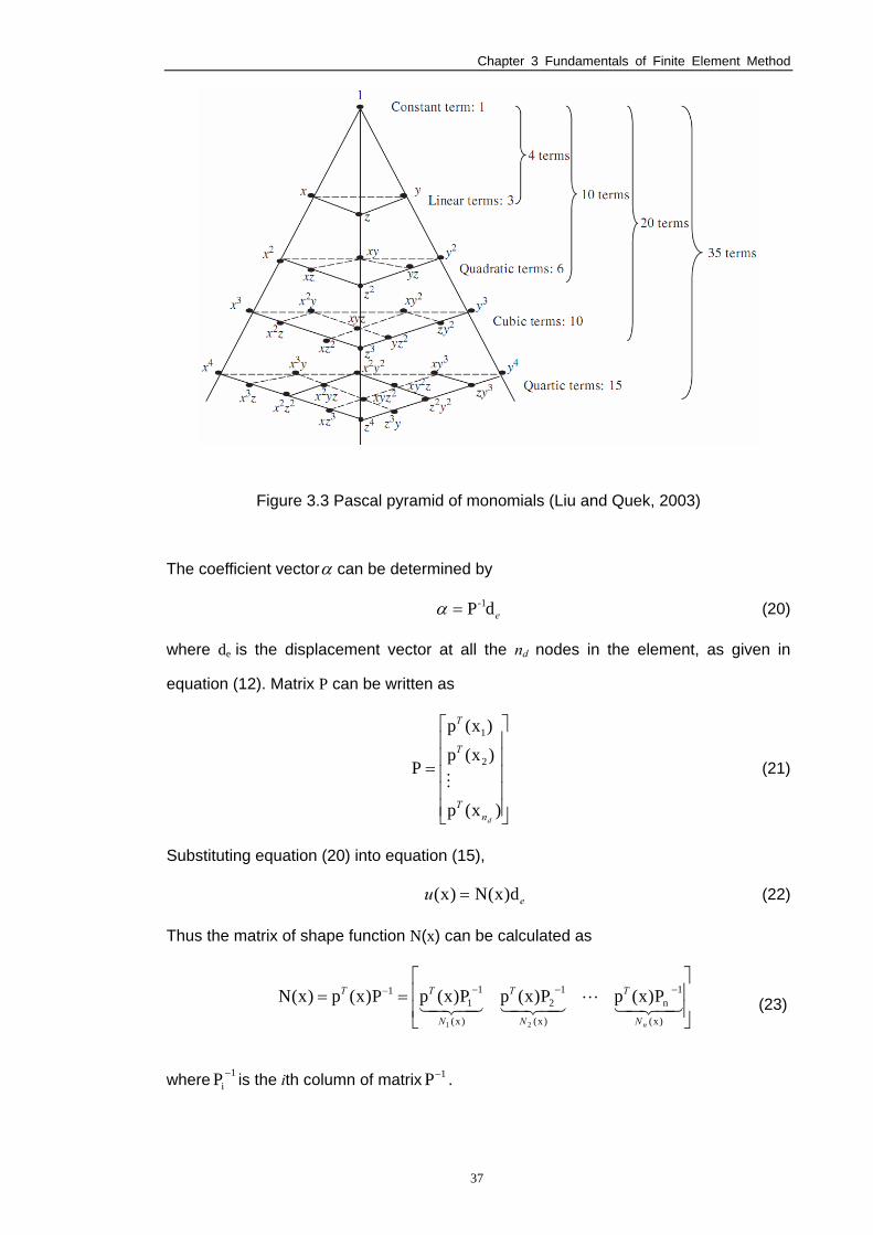
Chapter 3 Fundamentals of Finite Element Method
37
Figure 3.3 Pascal pyramid of monomials (Liu and Quek, 2003)
The coefficient vectorα can be determined by
edP-1=α (20)
where de is the displacement vector at all the nd nodes in the element, as given in
equation (12). Matrix P can be written as
⎥⎥⎥⎥⎥
⎦
⎤
⎢⎢⎢⎢⎢
⎣
⎡
=
)x(p
)x(p
)x(p
P 2
1
dnT
T
T
M (21)
Substituting equation (20) into equation (15),
eu d)x(N)x( = (22)
Thus the matrix of shape function N(x) can be calculated as
(23)
where 1iP − is the ith column of matrix 1P− .
⎥⎥
⎦
⎤
⎢⎢
⎣
⎡== −−−−
43421L
4342143421)x(
1n
)x(
12
)x(
11
1 P)x(pP)x(pP)x(pP)x(p)x(N21 nN
T
N
T
N
TT

Chapter 3 Fundamentals of Finite Element Method
38
3.2.4 Formation of Local FE Equations
Once the shape functions are constructed, the strain vector can be calculated as
eBd=ε (24)
where B is the strain matrix and defined by
LNB = (25)
in which L is a matrix of partial differential operator.
Substituting equation (24) into the strain energy term in (8)
eTT
eeTT
eT VVV dDBdBd
21dDBdBd
21dD
21
⎟⎠⎞⎜
⎝⎛===Π ∫∫∫ εε (26)
By denoting
∫= VT DBdBke (27)
which is called the element stiffness matrix, equation (26) can be rewritten as
eeT
e dkd21
=Π (28)
Similarly, by substituting equation (10) into the kinetic energy term in (7)
eTT
eeTT
eT VVVT dNdNd
21ddNNd
21dUU
21 &&&&&& ⎟
⎠⎞⎜
⎝⎛=== ∫∫∫ ρρρ (29)
By denoting
VT NdNme ∫= ρ (30)
which is known as mass matrix and the kinetic energy can be rewritten as
eeT
eT dmd21 &&= (31)
Finally, by substituting equation (10) into equation (9), the work done by external forces
can be expressed as
∫∫∫∫ +=+= )dfN(d)dfN(ddfUdfU fsTT
ebTT
efsT
bT
f SVSVW (32)
By denoting
∫= VbT
b dfNF (33)
fsT
s S∫= dfNF (34)
Chapter 3 Fundamentals of Finite Element Method
39
Then equation (32) can be rewritten as
eT
esT
ebT
efW fdFdFd =+= (35)
Fb and Fs are the forces acting on nodes of the elements. In terms of the work done by
these nodal forces, it is equivalent to the body forces and surface forces on the
elements. Hence, those nodal forces can be added up to form the total nodal force
sbe FFf += (36)
Substituting equations (28), (31) and (35) into (6)
(37)
Applying Hamilton’s Principle (5)
(38)
Since the variation and integration operators are interchangeable
(39)
The deriving from (38) to (39) can be found in Liu and Quek (2003). In equation (39), the
variation and differentiation with time are also interchangeable
( )Te
TeT
e ttd
dd
dddd δδδ =⎟⎟
⎠
⎞⎜⎜⎝
⎛=& (40)
Substituting equation (40) into (39) and integrating the first term
(41)
Because the initial condition at t1 and the final condition at t2 have to be satisfied for any
de, and no variation at t1 and t2 is allowed (Liu and Quek, 2003), 0d =eδ , the first term on
the right side of equation (41) vanishes.
Substituting equation (41) into (39) leads to
(42)
eT
eeeT
eeeT
eL fddkd21dmd
21
+−= &&
∫ =⎟⎠⎞
⎜⎝⎛ +−2
1
0dfddkd21dmd
21t
t eT
eeeT
eeeT
e t&&δ
( )∫ =+−2
1
0dfddkddmd e
t
t eT
eeeT
eeT
e tδδδ &&
tttt
t eeT
e
t
t eeT
ettee
Te
t
t eeT
e ddmdddmddmdddmd 2
1
2
1
2
1
2
1
0
∫∫∫ −=−==
&&&&43421&&& δδδδ
( )∫ =+−−2
1
0dfdkdmdt
t eeeeeT
e t&&δ

Chapter 3 Fundamentals of Finite Element Method
40
In order to have the integration in equation (42) as zero for an arbitrary integrand, the
integrand itself has to be zero
( ) 0fdkdmd e =+−− eeeeT
e&&δ (43)
Because of the arbitrary nature of the variation of the displacements, to satisfy equation
(43), we have
eeeee fdmdk =+ && (44)
3.2.5 Assembly of Global FE Equations
The element equation in (44) is formulated based on the local coordinate system of the
element. To assemble all the element equations to form the global system equations, a
coordinate transformation has to be carried out. By using the coordinate transformation,
the displacement vector de can be transferred into a displacement vector Ue oriented in
the global coordinate system.
ee TUd = (45)
where T is the transformation matrix. It can also be applied to transfer the force vector fe
in local coordinate system to force vector in global coordinate system.
ee TFf = (46)
Substituting equations (45) and (46) into (44), we have
eeeee FUMUK =+ && (47)
where
TkTK eT
e = (48)
TmTM eT
e = (49)
eT
e fTF = (50)
In the end, the FE equations of individual elements are assembled to form the global FE
system equation:
Chapter 3 Fundamentals of Finite Element Method
41
FUMKU =+ && (51)
where K and M are the global stiffness and mass matrix respectively, U is a vector of all
the displacements at all nodes, and F is a vector of all external nodal forces.
3.3 Different Types of Finite Elements
Since 3-D solid and 2-D structural elements are the most commonly used elements in
the FE analysis of metal forming process, the formulations of a 3-D solid element, a
shell element, as well as a 2-D plane stress/strain element and a plate element which
are used to generate the formulations of the shell element are discussed in this section.
3.3.1 3-D Solid Element
The 3-D solid element is the most general of all solid finite elements, as all its field
variables are dependent of x, y and z. A 3-D solid element can be a tetrahedron or
hexahedron in shape, where each node has three translational DOFs. Here, the 8
noded hexahedron element is taken as an example to explain the formulations of shape
function, strain matrix, stiffness matrix and mass matrix in the 3-D solid element.
As shown in Figure 3.4, a hexahedron element has eight nodes, numbered 1, 2, 3, 4
and 5, 6, 7, 8 in a counter-clockwise manner. Since each node has three DOFs, there
are total 24 DOFs in a hexahedron element. By using a natural coordinate system
(ξ ,η ,ζ ) with its origin at the centre of the element, it is easier to construct the shape
functions and to evaluate the matrix integration than using the physical coordinate
system ( x , y , z ). Assuming that the dimensions of the hexahedron element
is cba 222 ×× , the relationship between local natural coordinate system and physical
coordinate system is given by
ax=ξ , by=η , cz=ζ (52)
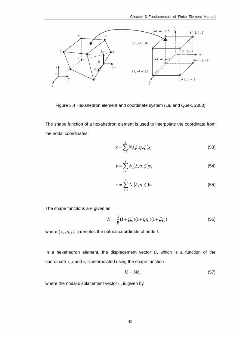
Chapter 3 Fundamentals of Finite Element Method
42
Figure 3.4 Hexahedron element and coordinate system (Liu and Quek, 2003)
The shape function of a hexahedron element is used to interpolate the coordinate from
the nodal coordinates:
( )∑=
=8
1
,,i
ii xNx ζηξ (53)
( )∑=
=8
1
,,i
ii yNy ζηξ (54)
( )∑=
=8
1
,,i
ii zNz ζηξ (55)
The shape functions are given as
)1)(1)(1(81
iiiiN ζζηηξξ +++= (56)
where ( iξ , iη , iζ ) denotes the natural coordinate of node i.
In a hexahedron element, the displacement vector U, which is a function of the
coordinate x, y and z, is interpolated using the shape function
eNdU = (57)
where the nodal displacement vector de is given by
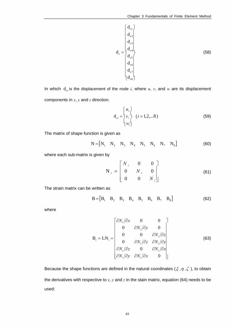
Chapter 3 Fundamentals of Finite Element Method
43
⎪⎪⎪⎪⎪
⎭
⎪⎪⎪⎪⎪
⎬
⎫
⎪⎪⎪⎪⎪
⎩
⎪⎪⎪⎪⎪
⎨
⎧
=
8
7
6
5
4
3
2
1
dddddddd
d
e
e
e
e
e
e
e
e
e (58)
In which eid is the displacement of the node i, where u, v, and w are its displacement
components in x, y and z direction.
⎪⎭
⎪⎬
⎫
⎪⎩
⎪⎨
⎧=
i
i
i
ei
wvu
d ( 8,...2,1=i ) (59)
The matrix of shape function is given as
[ ]87654321 NNNNNNNNN = (60)
where each sub-matrix is given by
⎥⎥⎥
⎦
⎤
⎢⎢⎢
⎣
⎡=
i
i
i
i
NN
N
000000
N (61)
The strain matrix can be written as
[ ]87654321 BBBBBBBBB = (62)
where
⎥⎥⎥⎥⎥⎥⎥⎥
⎦
⎤
⎢⎢⎢⎢⎢⎢⎢⎢
⎣
⎡
∂∂∂∂∂∂∂∂∂∂∂∂∂∂
∂∂∂∂
==
00
000
0000
LNB
xNyNxNzNyNzNzN
yNxN
ii
ii
ii
i
i
i
ii (63)
Because the shape functions are defined in the natural coordinates (ξ ,η ,ζ ), to obtain
the derivatives with respective to x, y and z in the stain matrix, equation (64) needs to be
used:
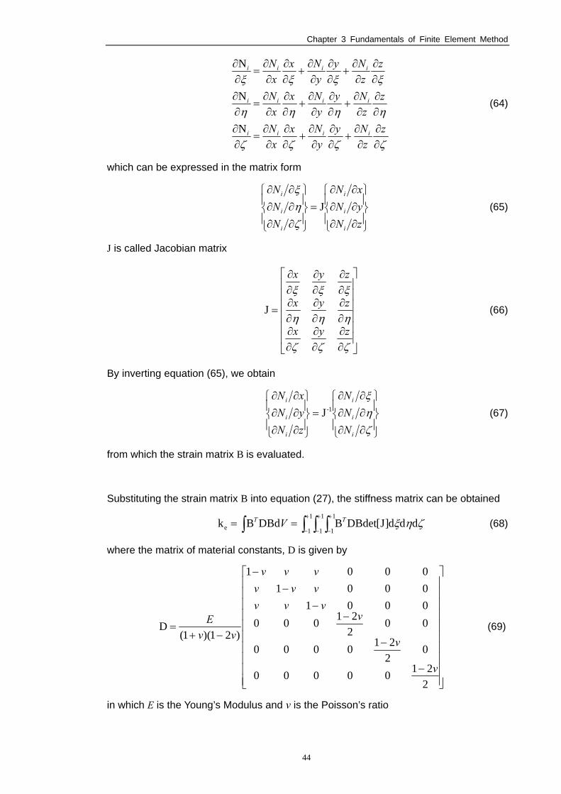
Chapter 3 Fundamentals of Finite Element Method
44
ζζζζ
ηηηη
ξξξξ
∂∂
∂∂
+∂∂
∂∂
+∂∂
∂∂
=∂∂
∂∂
∂∂
+∂∂
∂∂
+∂∂
∂∂
=∂∂
∂∂
∂∂
+∂∂
∂∂
+∂∂
∂∂
=∂∂
zz
Nyy
Nxx
N
zz
Nyy
Nxx
N
zz
Nyy
Nxx
N
iiii
iiii
iiii
N
N
N
(64)
which can be expressed in the matrix form
⎪⎭
⎪⎬
⎫
⎪⎩
⎪⎨
⎧
∂∂∂∂∂∂
=⎪⎭
⎪⎬
⎫
⎪⎩
⎪⎨
⎧
∂∂∂∂∂∂
zNyNxN
NNN
i
i
i
i
i
i
Jζηξ
(65)
J is called Jacobian matrix
⎥⎥⎥⎥⎥⎥
⎦
⎤
⎢⎢⎢⎢⎢⎢
⎣
⎡
∂∂
∂∂
∂∂
∂∂
∂∂
∂∂
∂∂
∂∂
∂∂
=
ζζζ
ηηη
ξξξ
zyx
zyx
zyx
J (66)
By inverting equation (65), we obtain
⎪⎭
⎪⎬
⎫
⎪⎩
⎪⎨
⎧
∂∂∂∂∂∂
=⎪⎭
⎪⎬
⎫
⎪⎩
⎪⎨
⎧
∂∂∂∂∂∂
ζηξ
i
i
i
i
i
i
NNN
zNyNxN
1-J (67)
from which the strain matrix B is evaluated.
Substituting the strain matrix B into equation (27), the stiffness matrix can be obtained
∫ ∫ ∫∫+
−
+
−
+
−==
1
1
1
1
1
1e ddd]J[DBdetBDBdBk ζηξTT V (68)
where the matrix of material constants, D is given by
⎥⎥⎥⎥⎥⎥⎥⎥⎥⎥
⎦
⎤
⎢⎢⎢⎢⎢⎢⎢⎢⎢⎢
⎣
⎡
−
−
−−
−−
−+=
22100000
02210000
00221000
000100010001
)21)(1(D
v
v
vvvv
vvvvvv
vvE
(69)
in which E is the Young’s Modulus and v is the Poisson’s ratio
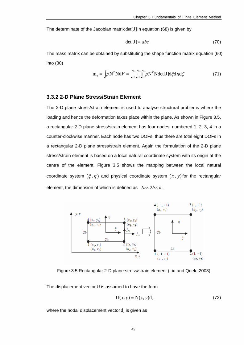
Chapter 3 Fundamentals of Finite Element Method
45
The determinate of the Jacobian matrix ]Jdet[ in equation (68) is given by
abc=]Jdet[ (70)
The mass matrix can be obtained by substituting the shape function matrix equation (60)
into (30)
∫ ∫ ∫∫+
−
+
−
+
−==
1
1
1
1
1
1e ddd]J[NdetNNdNm ζηξρρ TT V (71)
3.3.2 2-D Plane Stress/Strain Element
The 2-D plane stress/strain element is used to analyse structural problems where the
loading and hence the deformation takes place within the plane. As shown in Figure 3.5,
a rectangular 2-D plane stress/strain element has four nodes, numbered 1, 2, 3, 4 in a
counter-clockwise manner. Each node has two DOFs, thus there are total eight DOFs in
a rectangular 2-D plane stress/strain element. Again the formulation of the 2-D plane
stress/strain element is based on a local natural coordinate system with its origin at the
centre of the element. Figure 3.5 shows the mapping between the local natural
coordinate system (ξ ,η ) and physical coordinate system ( x , )y for the rectangular
element, the dimension of which is defined as hba ×× 22 .
Figure 3.5 Rectangular 2-D plane stress/strain element (Liu and Quek, 2003)
The displacement vector U is assumed to have the form
eyxyx d),(N),(U = (72)
where the nodal displacement vector ed is given as
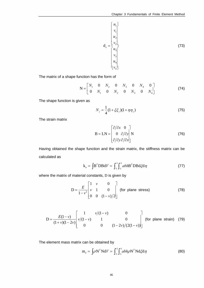
Chapter 3 Fundamentals of Finite Element Method
46
⎪⎪⎪⎪⎪
⎭
⎪⎪⎪⎪⎪
⎬
⎫
⎪⎪⎪⎪⎪
⎩
⎪⎪⎪⎪⎪
⎨
⎧
=
4
4
3
3
2
2
1
1
d
vuvuvuvu
e (73)
The matrix of a shape function has the form of
⎥⎦
⎤⎢⎣
⎡=
4321
4321
00000000
NNNNN
NNNN (74)
The shape function is given as
)1)(1(41
jjjN ηηξξ ++= (75)
The strain matrix
N0
0LNB⎥⎥⎥
⎦
⎤
⎢⎢⎢
⎣
⎡
∂∂∂∂
∂∂
∂∂==
xy
y
x (76)
Having obtained the shape function and the strain matrix, the stiffness matrix can be
calculated as
ηξdDBdBDBdBk1
1
1
1eTT abhV ∫ ∫∫
+
−
+
−== (77)
where the matrix of material constants, D is given by
⎥⎥⎥
⎦
⎤
⎢⎢⎢
⎣
⎡
−−
=2)1(00
0101
1D 2
vv
v
vE
(for plane stress) (78)
⎥⎥⎥
⎦
⎤
⎢⎢⎢
⎣
⎡
−−−
−
−+−
=))1(2()21(00
01)1(0)1(1
)21)(1()1(D
vvvv
vv
vvvE
(for plane strain) (79)
The element mass matrix can be obtained by
∫ ∫∫+
−
+
−==
1
1
1
1e dNdNNdNm ηξρρ TT abhV (80)
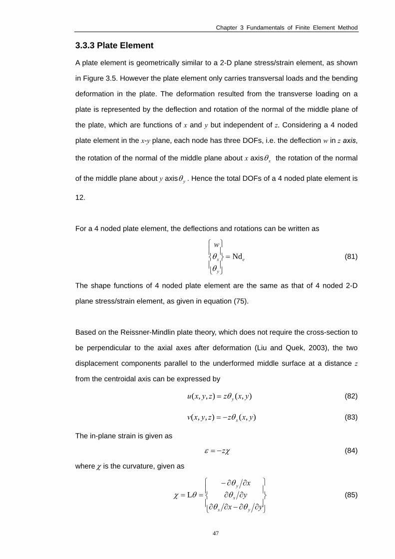
Chapter 3 Fundamentals of Finite Element Method
47
3.3.3 Plate Element
A plate element is geometrically similar to a 2-D plane stress/strain element, as shown
in Figure 3.5. However the plate element only carries transversal loads and the bending
deformation in the plate. The deformation resulted from the transverse loading on a
plate is represented by the deflection and rotation of the normal of the middle plane of
the plate, which are functions of x and y but independent of z. Considering a 4 noded
plate element in the x-y plane, each node has three DOFs, i.e. the deflection w in z axis,
the rotation of the normal of the middle plane about x axis xθ the rotation of the normal
of the middle plane about y axis yθ . Hence the total DOFs of a 4 noded plate element is
12.
For a 4 noded plate element, the deflections and rotations can be written as
e
y
x
wNd=
⎪⎭
⎪⎬
⎫
⎪⎩
⎪⎨
⎧
θθ (81)
The shape functions of 4 noded plate element are the same as that of 4 noded 2-D
plane stress/strain element, as given in equation (75).
Based on the Reissner-Mindlin plate theory, which does not require the cross-section to
be perpendicular to the axial axes after deformation (Liu and Quek, 2003), the two
displacement components parallel to the underformed middle surface at a distance z
from the centroidal axis can be expressed by
),(),,( yxzzyxu yθ= (82)
),(),,( yxzzyxv xθ−= (83)
The in-plane strain is given as
χε z−= (84)
where χ is the curvature, given as
⎪⎭
⎪⎬
⎫
⎪⎩
⎪⎨
⎧
∂∂−∂∂∂∂∂∂−
==yx
yx
yx
x
y
θθθθ
θχ L (85)
Chapter 3 Fundamentals of Finite Element Method
48
The off-plane shear strain is given as
⎪⎪⎭
⎪⎪⎬
⎫
⎪⎪⎩
⎪⎪⎨
⎧
∂∂
+−
∂∂
+=
⎭⎬⎫
⎩⎨⎧
=
yw
xw
x
y
yz
xz
θ
θ
ξξ
γ (86)
Hamilton’s Principle is used to derive the equation of motion. The strain energy of a 4
noded plate element can be obtained as
∫ ∫∫ ∫ +=ΠA
h T
A
h T AzAz00
dd21dd
21 γτσε (87)
whereτ is the average shear stresses related to the shear strain in the form
γκγκττ
τ syz
xz
GG
D0
0=⎥
⎦
⎤⎢⎣
⎡=
⎭⎬⎫
⎩⎨⎧
= (88)
in whichG is the shear modulus, andκ is a constant that is usually taken to be 122π
(Liu and Quek, 2003). Substituting equation (84) and (88) into (87), the strain energy
becomes
∫∫ +=ΠA s
T
A
T AhAh dD21dD
1221 3
γγκχχ (89)
The kinetic energy of the plate element is given by
( ) VwvuT d21 222∫ ++= &&&ρ (90)
which is a summation of the contributions of three velocity components in
the x , y and z directions. Substituting equation (82) and (83) into (90), the kinetic energy
can be obtained (Liu and Quek, 2003)
∫∫ =++= AAhhwhT Tyx d)Idd(
21d)
1212(
21 2
32
32 θθρ &&& (91)
where
⎥⎥⎥
⎦
⎤
⎢⎢⎢
⎣
⎡=
1200012000
I3
3
hh
h
ρρ
ρ (92)
To obtain the shape function, substituting equation (81) into (87) will lead to
[ ] [ ]∫∫ +=A s
T
A
Te AhAh dBDBdDBB
12k OOII
3
κ (93)
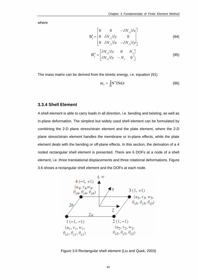
Chapter 3 Fundamentals of Finite Element Method
49
where
⎥⎥⎥
⎦
⎤
⎢⎢⎢
⎣
⎡
∂∂−∂∂∂∂
∂∂−=
yNxNyN
xN
jj
j
j
000
00BI
j (94)
⎥⎦
⎤⎢⎣
⎡−∂∂
∂∂=
00
BOj
jj
jj
NyNNxN
(95)
The mass matrix can be derived from the kinetic energy, i.e. equation (91)
∫= Ae AINdNm T (96)
3.3.4 Shell Element
A shell element is able to carry loads in all direction, i.e. bending and twisting, as well as
in-plane deformation. The simplest but widely used shell element can be formulated by
combining the 2-D plane stress/strain element and the plate element, where the 2-D
plane stress/strain element handles the membrane or in-plane effects, while the plate
element deals with the bending or off-plane effects. In this section, the derivation of a 4
noded rectangular shell element is presented. There are 6 DOFs at a node of a shell
element, i.e. three translational displacements and three rotational deformations. Figure
3.6 shows a rectangular shell element and the DOFs at each node.
Figure 3.6 Rectangular shell element (Liu and Quek, 2003)
Chapter 3 Fundamentals of Finite Element Method
50
The nodal displacement vector of a rectangular shell element can be written as
⎪⎪⎭
⎪⎪⎬
⎫
⎪⎪⎩
⎪⎪⎨
⎧
=
4
3
2
1
dddd
d
e
e
e
e
e (97)
where eid are the displacement vector at node i
⎪⎪⎪⎪
⎭
⎪⎪⎪⎪
⎬
⎫
⎪⎪⎪⎪
⎩
⎪⎪⎪⎪
⎨
⎧
=
zi
yi
xi
i
i
i
ei
wvu
θ
θθ
d (98)
The stiffness matrix of a 2-D solid rectangular element is used to deal with the
membrane effects of a rectangular shell element
⎥⎥⎥⎥⎥
⎦
⎤
⎢⎢⎢⎢⎢
⎣
⎡
=
m44
m43
m42
m41
m34
m33
m32
m31
m24
m23
m22
m21
m14
m13
m12
m11
me
kkkkkkkkkkkkkkkk
k (99)
where the superscript m represents the membrane matrix. Each sub-matrix has a
dimension of 2×2, as it corresponds to the two DOFs u and v at each node.
The stiffness matrix of a rectangular plate element is used to take account the bending
effects in a rectangular shell element
⎥⎥⎥⎥⎥
⎦
⎤
⎢⎢⎢⎢⎢
⎣
⎡
=
b44
b43
b42
b41
b34
b33
b32
b31
b24
b23
b22
b21
b14
b13
b12
b11
be
kkkkkkkkkkkkkkkk
k (100)
where the superscript b stands for the bending matrix. Each sub-matrix has a dimension

Chapter 3 Fundamentals of Finite Element Method
51
of 3×3, corresponding to three DOFs, i.e. w, xθ and yθ .
The stiffness matrix of a rectangular shell element in the local coordinate system is then
formulated by combining equation (99) and (100):
⎥⎥⎥⎥⎥⎥⎥⎥⎥⎥⎥⎥⎥⎥⎥⎥⎥
⎦
⎤
⎢⎢⎢⎢⎢⎢⎢⎢⎢⎢⎢⎢⎢⎢⎢⎢⎢
⎣
⎡
=
0000000000000k00k00k00k000k00k00k00k0000000000000k00k00k00k000k00k00k00k0000000000000k00k00k00k000k00k00k00k0000000000000k00k00k00k000k00k00k00k
k
b44
b43
b42
b41
m44
m43
m42
m41
b34
b33
b32
b31
m34
m33
m32
m31
b24
b23
b22
b21
m24
m23
m22
m21
b14
b13
b12
b11
m14
m13
m12
m11
e (101)
Similarly, the mass matrix of a rectangular shell element can be obtained by combining
the mass matrices of a 2-D rectangular solid element and a rectangular plate element.
3.4 Non-linear Solution Method
In this section, two non-linear FE solution method, i.e. static implicit method and
dynamic explicit method are summarised.
3.4.1 Implicit Method Newton-Raphson method is one of the most commonly used solution procedures in
non-linear implicit analysis (Harewood and McHugh, 2007). Unlike solving a linear
problem, the solution cannot be obtained by solving a single system of equations for the
non-linear problem. Hence, in the non-linear implicit analysis, the loading is applied
gradually and incrementally. Normally, the simulation breaks into a number of load
increments and finds the approximate equilibrium at the end of the each increment. It
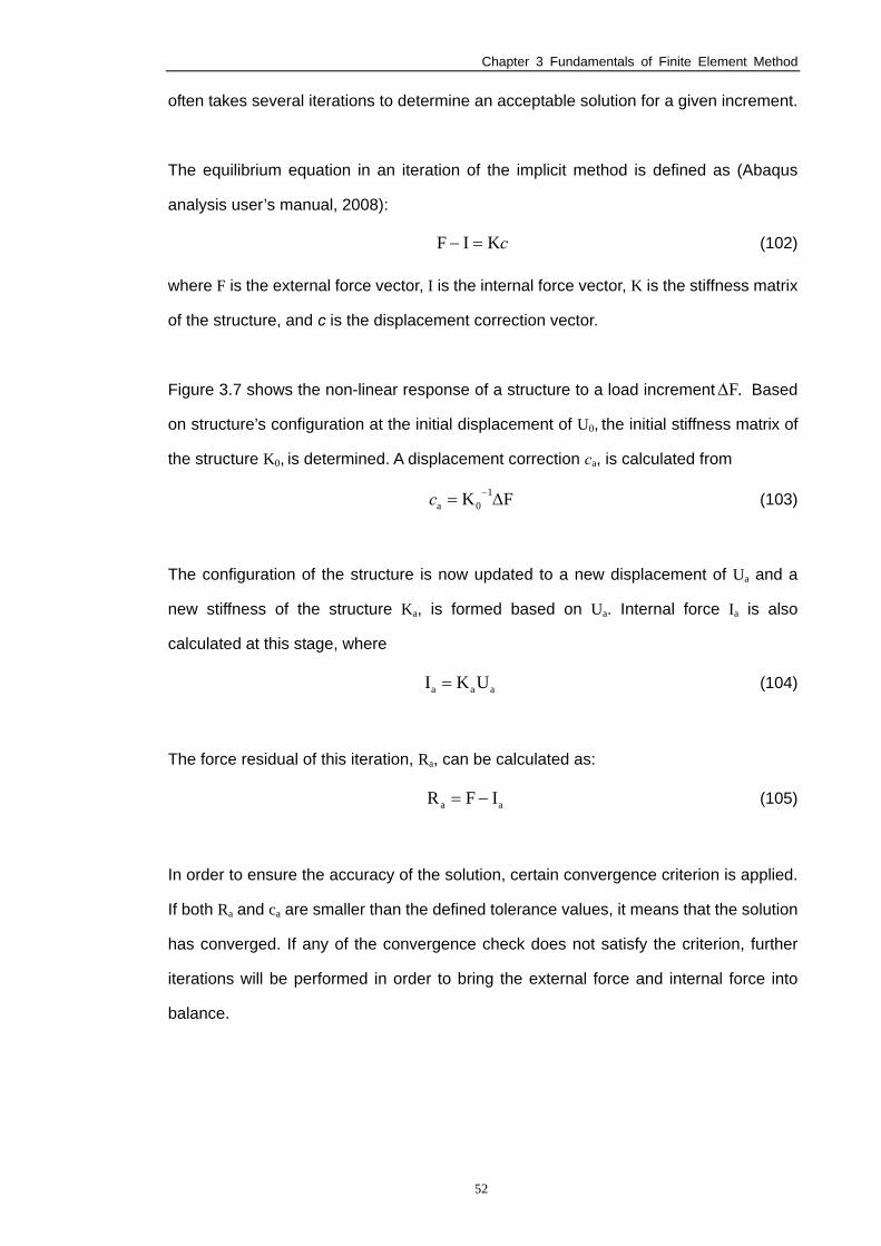
Chapter 3 Fundamentals of Finite Element Method
52
often takes several iterations to determine an acceptable solution for a given increment.
The equilibrium equation in an iteration of the implicit method is defined as (Abaqus
analysis user’s manual, 2008):
cKIF =− (102)
where F is the external force vector, I is the internal force vector, K is the stiffness matrix
of the structure, and c is the displacement correction vector.
Figure 3.7 shows the non-linear response of a structure to a load increment .FΔ Based
on structure’s configuration at the initial displacement of U0, the initial stiffness matrix of
the structure K0, is determined. A displacement correction ca, is calculated from
FK 10a Δ= −c (103)
The configuration of the structure is now updated to a new displacement of Ua and a
new stiffness of the structure Ka, is formed based on Ua. Internal force Ia is also
calculated at this stage, where
aaa UKI = (104)
The force residual of this iteration, Ra, can be calculated as:
aa IFR −= (105)
In order to ensure the accuracy of the solution, certain convergence criterion is applied.
If both Ra and ca are smaller than the defined tolerance values, it means that the solution
has converged. If any of the convergence check does not satisfy the criterion, further
iterations will be performed in order to bring the external force and internal force into
balance.
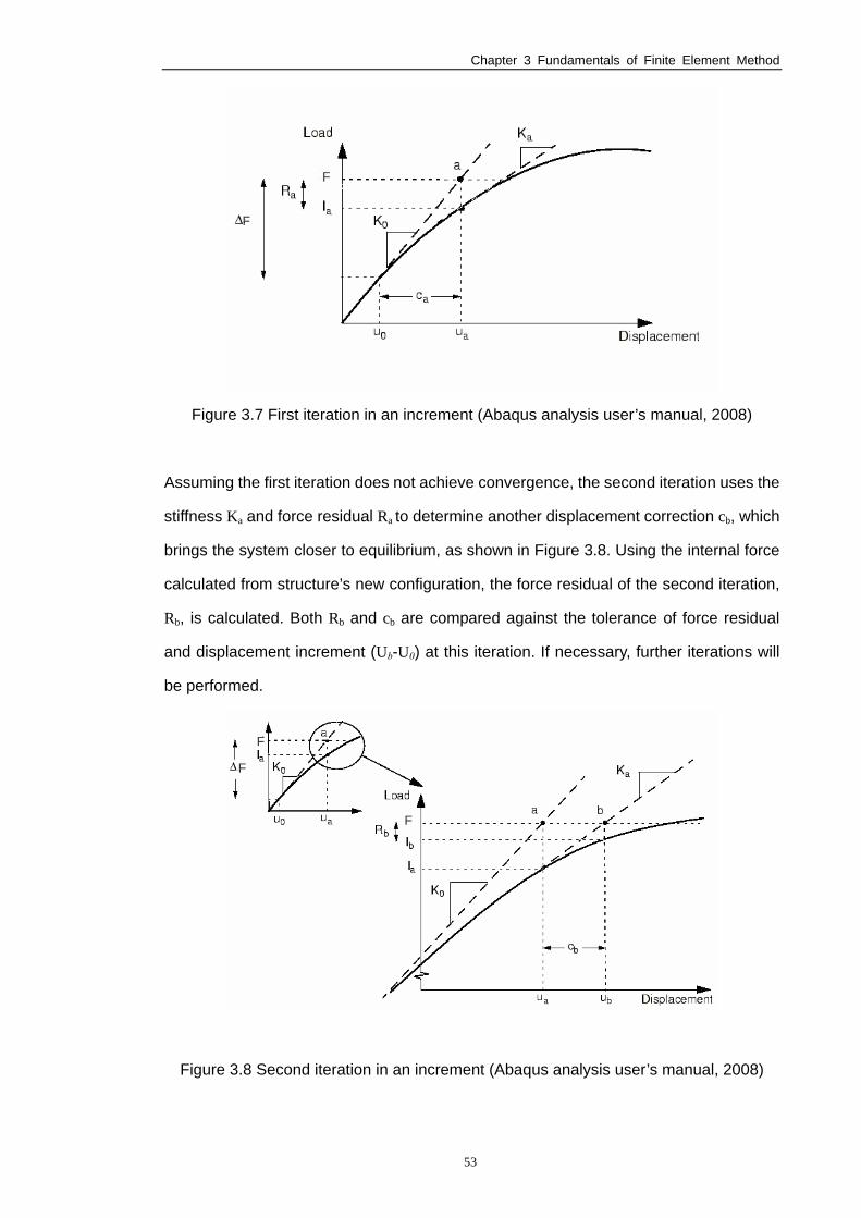
Chapter 3 Fundamentals of Finite Element Method
53
Figure 3.7 First iteration in an increment (Abaqus analysis user’s manual, 2008)
Assuming the first iteration does not achieve convergence, the second iteration uses the
stiffness Ka and force residual Ra to determine another displacement correction cb, which
brings the system closer to equilibrium, as shown in Figure 3.8. Using the internal force
calculated from structure’s new configuration, the force residual of the second iteration,
Rb, is calculated. Both Rb and cb are compared against the tolerance of force residual
and displacement increment (Ub-U0) at this iteration. If necessary, further iterations will
be performed.
Figure 3.8 Second iteration in an increment (Abaqus analysis user’s manual, 2008)
F
F
F
F
F
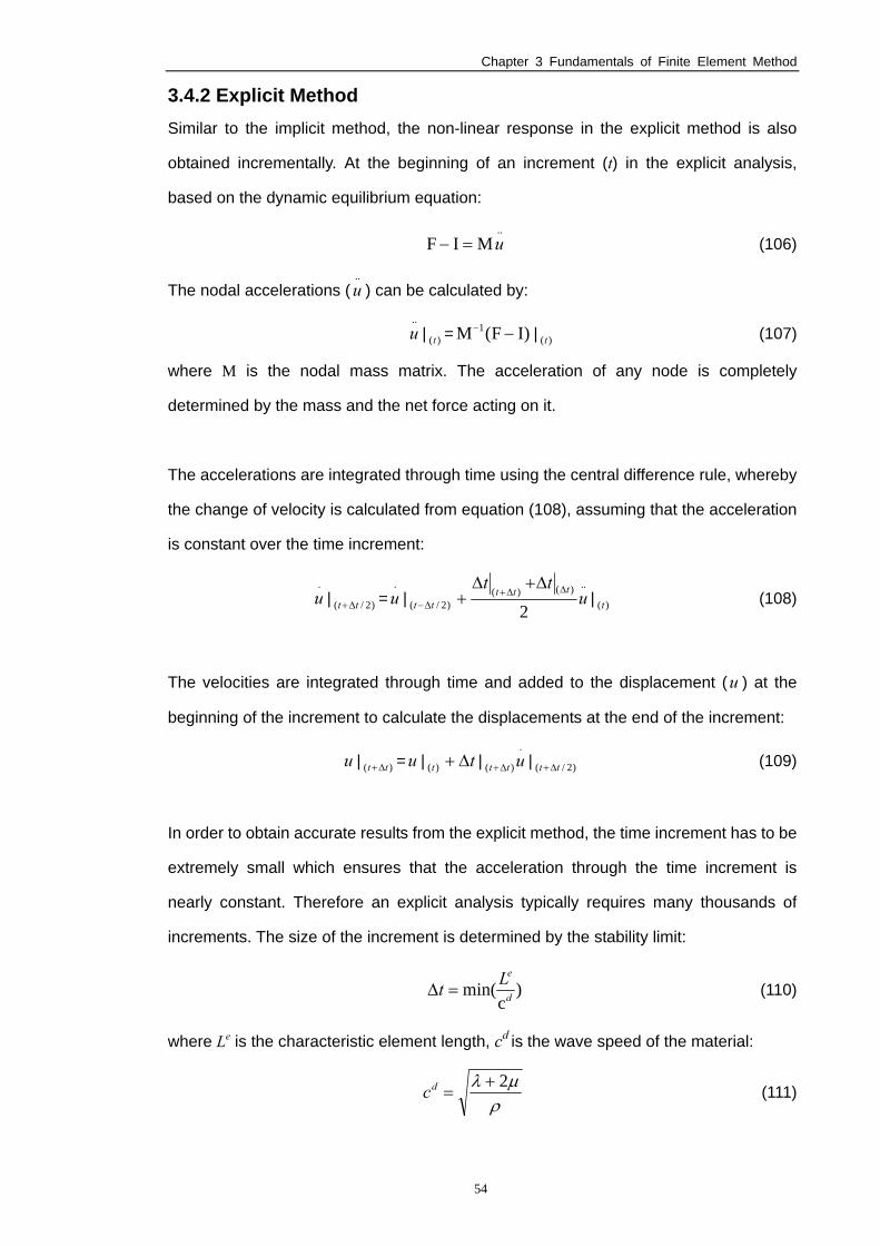
Chapter 3 Fundamentals of Finite Element Method
54
3.4.2 Explicit Method Similar to the implicit method, the non-linear response in the explicit method is also
obtained incrementally. At the beginning of an increment (t) in the explicit analysis,
based on the dynamic equilibrium equation:
..MIF u=− (106)
The nodal accelerations (..u ) can be calculated by:
..u | )(t = )IF(M 1 −− | )(t (107)
where M is the nodal mass matrix. The acceleration of any node is completely
determined by the mass and the net force acting on it.
The accelerations are integrated through time using the central difference rule, whereby
the change of velocity is calculated from equation (108), assuming that the acceleration
is constant over the time increment:
.u | )2/( tt Δ+ =
.u | )2/( tt Δ−
..)()(
2u
tt ttt ΔΔ+Δ+Δ
+ | )(t (108)
The velocities are integrated through time and added to the displacement (u ) at the
beginning of the increment to calculate the displacements at the end of the increment:
u | )( tt Δ+ =u | )(t tΔ+ |.
)( utt Δ+ | )2/( tt Δ+ (109)
In order to obtain accurate results from the explicit method, the time increment has to be
extremely small which ensures that the acceleration through the time increment is
nearly constant. Therefore an explicit analysis typically requires many thousands of
increments. The size of the increment is determined by the stability limit:
)c
min( d
eLt =Δ (110)
where Le is the characteristic element length, cd is the wave speed of the material:
ρμλ 2+
=dc (111)
Chapter 3 Fundamentals of Finite Element Method
55
where λ and μ are Lamé’s elastic constants. If T is the actual time of the analysed
process, the number of time increments required n can be obtained by:
)2
min(μλ
ρ+
×=
Δ=
eL
Tt
Tn (112)
Normally it is unfeasible to run a quasi-static analysis with its real time scale, as the
computing time is extremely long (Harewood and McHugh, 2007). Two techniques have
been used to speed up the analysis: the first method is by artificially increasing the
loading or deformation rate, known as load rate scaling; the second method is to
increase the density of the material, known as mass scaling. According to equations
(110) - (112), mass scaling by a factor of q2 should have the same speeding up effects
as load rate scaling by a factor of q. Mass scaling is preferable as it does not affect the
mechanical response of rate-dependent material (Tekkaya, 2000). Nevertheless, if a
very large speed-up factor is applied, the corresponding inertial forces will affect the
mechanical response and produce unrealistic dynamic results. The general rule to
control the inertial effects resulting from mass scaling is to ensure that the kinetic energy
of the material should not exceed a small portion (typically 5%-10%) of its internal
energy during the majority of the duration of the process (Abaqus analysis user’s
manual, 2008).
3.5 Material Constitutive Model
3.5.1 von Mises Yield Criterion
Figure 3.9 shows a idealised bi-linear stress-strain curve, where the material behaves
elastically until the initial yielding stress yσ is reached (Dunne and Petrinic, 2005). If at a
strain of ε the load is reversed (unloading), the stress-strain response is assumed to
follow the elastic law, i.e. the gradient of the unloading stress-strain curve is again the
Young’s modulus E, as it is in the elastic loading process. Once a stress of zero is
obtained, the remaining strain is the plastic strain pε and the recovered strain is the
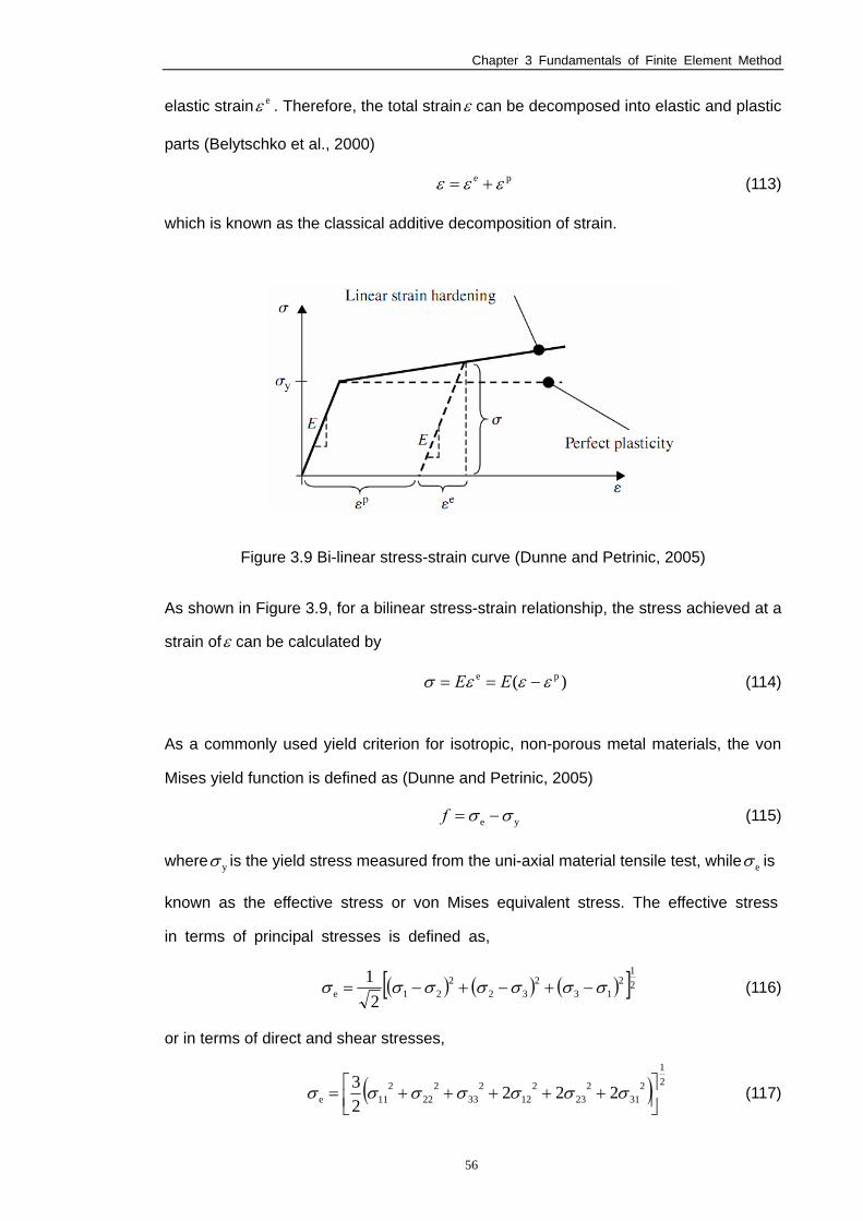
Chapter 3 Fundamentals of Finite Element Method
56
elastic strain eε . Therefore, the total strainε can be decomposed into elastic and plastic
parts (Belytschko et al., 2000)
pe εεε += (113)
which is known as the classical additive decomposition of strain.
Figure 3.9 Bi-linear stress-strain curve (Dunne and Petrinic, 2005)
As shown in Figure 3.9, for a bilinear stress-strain relationship, the stress achieved at a
strain ofε can be calculated by
)( pe εεεσ −== EE (114)
As a commonly used yield criterion for isotropic, non-porous metal materials, the von
Mises yield function is defined as (Dunne and Petrinic, 2005)
ye σσ −=f (115)
where yσ is the yield stress measured from the uni-axial material tensile test, while eσ is
known as the effective stress or von Mises equivalent stress. The effective stress
in terms of principal stresses is defined as,
( ) ( ) ( )[ ]21213
232
221e 2
1 σσσσσσσ −+−+−= (116)
or in terms of direct and shear stresses,
( ) 21
231
223
212
233
222
211e 222
23
⎥⎦⎤
⎢⎣⎡ +++++= σσσσσσσ (117)
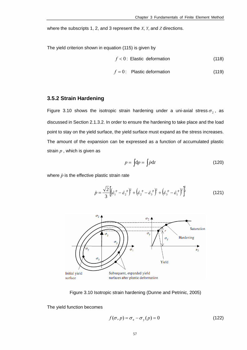
Chapter 3 Fundamentals of Finite Element Method
57
where the subscripts 1, 2, and 3 represent the X, Y, and Z directions.
The yield criterion shown in equation (115) is given by
0<f : Elastic deformation (118)
0=f : Plastic deformation (119)
3.5.2 Strain Hardening
Figure 3.10 shows the isotropic strain hardening under a uni-axial stress 2σ , as
discussed in Section 2.1.3.2. In order to ensure the hardening to take place and the load
point to stay on the yield surface, the yield surface must expand as the stress increases.
The amount of the expansion can be expressed as a function of accumulated plastic
strain p , which is given as
∫ ∫== tppp dd & (120)
where p& is the effective plastic strain rate
( ) ( ) ( )[ ]212p1
p3
2p3
p2
2p2
p13
2 εεεεεε &&&&&&& −+−+−=p (121)
Figure 3.10 Isotropic strain hardening (Dunne and Petrinic, 2005)
The yield function becomes
0)(),( ye =−= ppf σσσ (122)
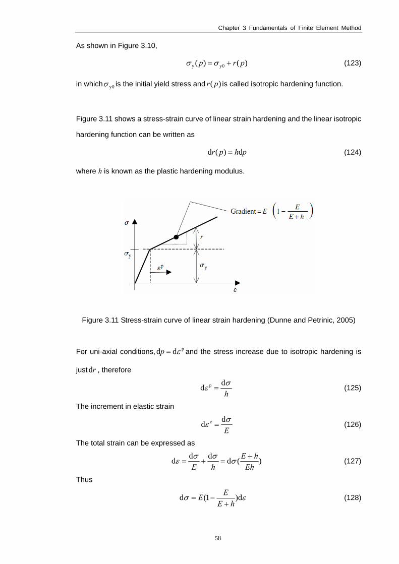
Chapter 3 Fundamentals of Finite Element Method
58
As shown in Figure 3.10,
)()( 0yy prp +=σσ (123)
in which 0yσ is the initial yield stress and )( pr is called isotropic hardening function.
Figure 3.11 shows a stress-strain curve of linear strain hardening and the linear isotropic
hardening function can be written as
phpr d)(d = (124)
where h is known as the plastic hardening modulus.
Figure 3.11 Stress-strain curve of linear strain hardening (Dunne and Petrinic, 2005)
For uni-axial conditions, pdd ε=p and the stress increase due to isotropic hardening is
just rd , therefore
hσε dd p = (125)
The increment in elastic strain
Eσε dd e = (126)
The total strain can be expressed as
)(ddddEh
hEhE
+=+= σσσε (127)
Thus
εσ d)1(dhE
EE+
−= (128)
Chapter 3 Fundamentals of Finite Element Method
59
3.6 Contact algorithms
Contact simulation, which is among the most difficult aspects for non-linear FE problems,
is also implemented in an incremental manner (Belytschko et al., 2000). In each time
increment of a metal forming problem simulation, there are three main aspects of the
contact modellling: identifying the area on the surfaces that are in contact; calculating
the contact force in the normal direction of the surfaces due to penetrations; thereafter
calculating the tangential force caused by friction. Four corresponding contact
formulations, i.e. contact surface weighting, tracking approach, constraint enforcement
method, and friction models, are discussed in this section.
3.6.1 Contact Surface Weighting To analyse the contact problem, master and slave surfaces have to be defined. The
master surface is the surface with “hard” material, for instance, the tools in the metal
forming simulation; whereas the slave surface is the surface with relatively “soft”
material such as the deformable blank. In general, there are two kinds of contact
weighting methods, i.e. a pure master-slave surface weighting and a balanced
master-slave surface weighting. In the pure master-slave surface weighting method,
only the penetrations of slave nodes into master surface will be resisted. There is no
restriction for the master surface to penetrate into the slave surface. Conversely, the
balanced master-surface weighting applies the pure master-slave weighting twice,
reversing the surfaces on the second pass, which minimises the penetrations of the
contact bodies. Therefore it provides more accurate results than the pure master-slave
surface in most cases and should be used whenever possible. The pure master-slave
surface weighting is used in the case such as when a rigid surface contacts a
deformable surface.
3.6.2 Tracking Approach
In the simulation of the contact / impact problem, a node on a contact surface is possible
to contact any facet on the opposite contact surface. There are two commonly used
Chapter 3 Fundamentals of Finite Element Method
60
contact tracking approaches, i.e. global search and local search (ABAQUS analysis
user’s manual, 2008). At the beginning of the simulation, an exhaustive global search is
carried out to determine the closet master surface facet for each slave node of each
contact pair. As the computing cost of global search is relatively high, a global search is
only conducted every few hundred time increments in a contact / impact model.
Conversely, a less expensive local search is performed in most time increments, where
a given slave node only searches the facets which are attached to the previous tracked
master surface node to determine the closest facet. Because the time increments are
small in most situations, the movement amongst contacting bodies is very limited from
one increment to the next and the local search is adequate to track the motion of the
contact surfaces.
3.6.3 Constraint Enforcement Method
In the simulation of contact problem, two methods to enforce contact conditions have
been commonly used, i.e. a kinematic predictor/corrector method and a penalty method
(ABAQUS analysis user’s manual, 2008). By using the kinematic contact method, the
kinematic state of the model is first advanced without considering the contact conditions
in each increment of the analysis. If the slave nodes penetrate into the master surface,
the time increment, the depth of the penetration of each node, the mass associated with
it will be used to calculate the resisting force to oppose the penetration. This resisting
force will make the slave nodes to exactly contact with the master surface. In other
words, no penetration of slave nodes into the master surface is allowed in the kinematic
contact method. The penalty contact applies less stringent enforcement of contact
constraints than the kinematic contact method. It searches for the slave node
penetration in the current configuration. Contact forces, which calculated as the
penetration distance times the penalty stiffness, are applied to the slave nodes to
oppose the penetration. At the same time, opposite forces act on the master surface at
the penetration point.
Chapter 3 Fundamentals of Finite Element Method
61
3.6.4 Frictional Model Apart from the normal forces, when surfaces are in contact, they normally transmit
shear forces across their interface as well. Coulomb friction is a common friction model
used to describe the interaction between two contacting surfaces. The tangential motion
will not start until the frictional shear stress reaches a critical value ( critτ ), which is
defined by:
pcrit ⋅= μτ (129)
whereμ is the coefficient of friction and p is the normal contact pressure. If the shear
stress is below critτ , there will no relative motion between the contact surfaces (sticking).
While when the frictional shear stress reaches its critical value relative motion (slipping)
occurs.
3.7 Summary
In this chapter, the fundamental theory of Finite Element Method, such as Hamilton’s
Principle and basic analysis procedure of FEM, has been discussed. The formulations
of four different types of finite elements, i.e. 3-D solid element, 2-D plane stress/strain
element, plate element and shell element, are presented. Two commonly used
non-linear FE solution methods, implicit method and explicit method, are compared.
Additionally, the elastic-plastic material constitutive model and contact algorithms of FE
simulation have been briefly outlined. Furthermore, the application of FEM to the metal
spinning simulation, e.g. development and verification of the metal spinning FE models,
are given in Section 4.2, 5.3 and 6.3 of the following chapters.
Chapter 4 Effects of Roller Path Profiles on Material Deformation
62
4. Effects of Roller Path Profiles on Material
Deformation
Until recently, the limited research work on the roller path profiles have been mainly
carried out by means of experimental investigation alone (Hayama et al., 1970) or by
simplified 2-D FE simulation (Liu et al., 2002). Possible causes of wall thinning in the
workpiece during conventional spinning are still not fully understood. For this reason,
four representative roller path profiles, i.e. combined concave and convex, convex,
linear, and concave curves, have been designed and used to carry out experimental
investigation in this study. 3-D elastic-plastic FE models of metal spinning have been
developed by using commercial FE software - Abaqus. The FE models have been
verified by conducting mesh convergence study, evaluating scaling techniques, and
comparing dimensional results. Finally, effects of these roller path profiles on the
variations of tool force, stress, wall thickness, and strain in the conventional spinning
have been analysed numerically. The results show that using a concave path produces
relatively high tool forces, stresses and reduction in wall thickness, comparing with the
corresponding results obtained from other roller paths. Conversely, low tool forces,
stresses and wall thinning are obtained in the FE model using a convex roller path.
4.1 Experimental Investigation
4.1.1 Experimental Setup By using the commercial spinning Computer-Aided Manufacturing (CAM) software -
OPUS, CNC programs of various roller passes have been developed. Figure 4.1
illustrates the setup and the schematic diagram of the spinning experiment, where the
angle between the roller axis and the mandrel axis is 45°. The blank is made of mild
steel (DC01) and its diameter and thickness are 240 mm and 2 mm, respectively. A feed
rate of 800 mm/min and a spindle speed of 400 rpm are chosen for all the experimental
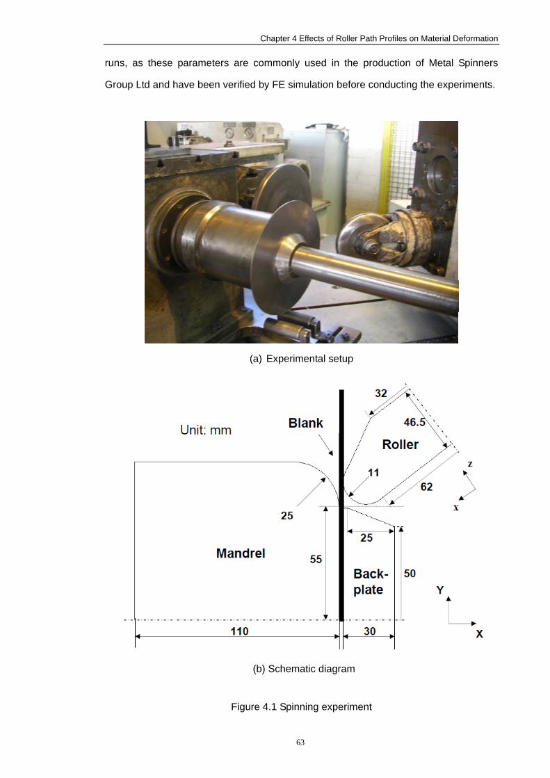
Chapter 4 Effects of Roller Path Profiles on Material Deformation
63
runs, as these parameters are commonly used in the production of Metal Spinners
Group Ltd and have been verified by FE simulation before conducting the experiments.
(a) Experimental setup
(b) Schematic diagram
Figure 4.1 Spinning experiment
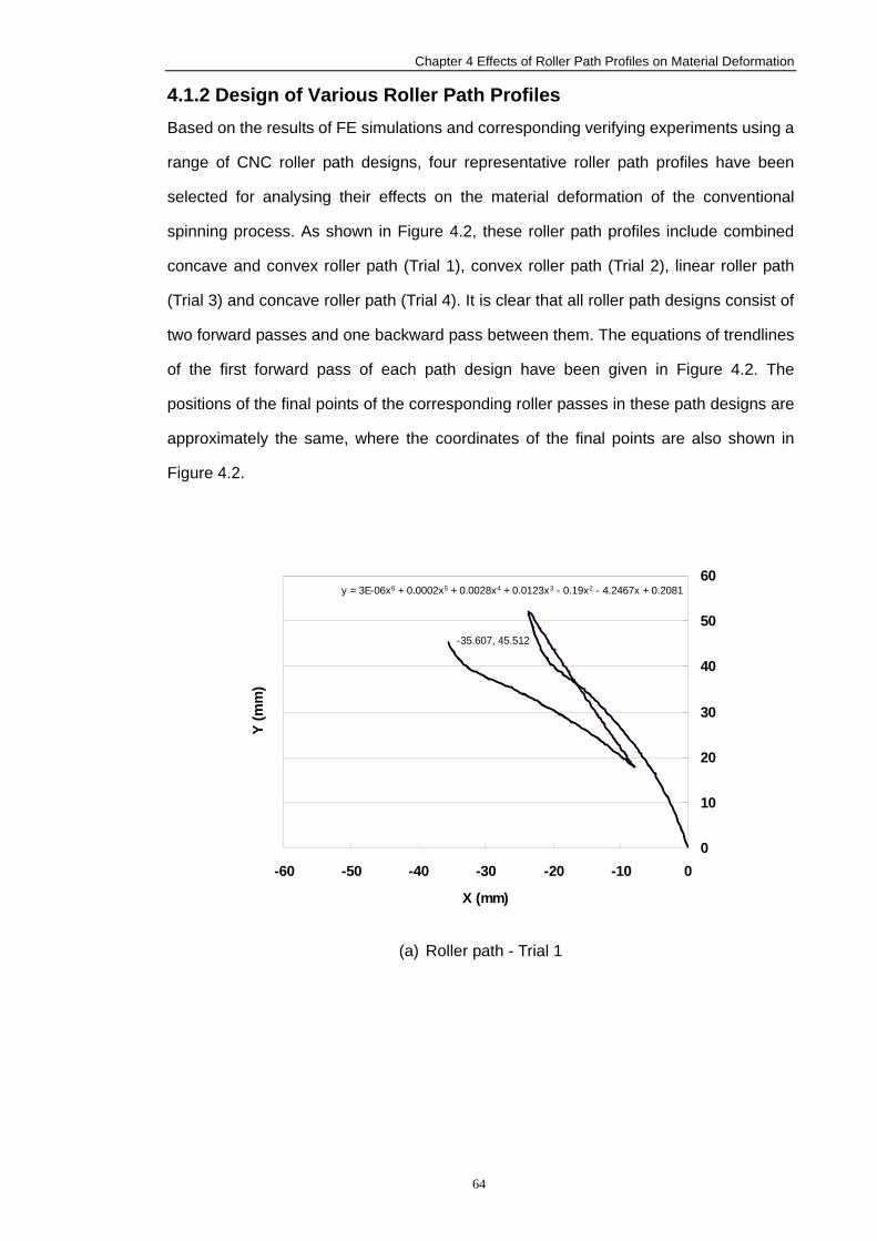
Chapter 4 Effects of Roller Path Profiles on Material Deformation
64
4.1.2 Design of Various Roller Path Profiles Based on the results of FE simulations and corresponding verifying experiments using a
range of CNC roller path designs, four representative roller path profiles have been
selected for analysing their effects on the material deformation of the conventional
spinning process. As shown in Figure 4.2, these roller path profiles include combined
concave and convex roller path (Trial 1), convex roller path (Trial 2), linear roller path
(Trial 3) and concave roller path (Trial 4). It is clear that all roller path designs consist of
two forward passes and one backward pass between them. The equations of trendlines
of the first forward pass of each path design have been given in Figure 4.2. The
positions of the final points of the corresponding roller passes in these path designs are
approximately the same, where the coordinates of the final points are also shown in
Figure 4.2.
-35.607, 45.512
y = 3E-06x6 + 0.0002x5 + 0.0028x4 + 0.0123x3 - 0.19x2 - 4.2467x + 0.2081
0
10
20
30
40
50
60
-60 -50 -40 -30 -20 -10 0
X (mm)
Y (m
m)
(a) Roller path - Trial 1
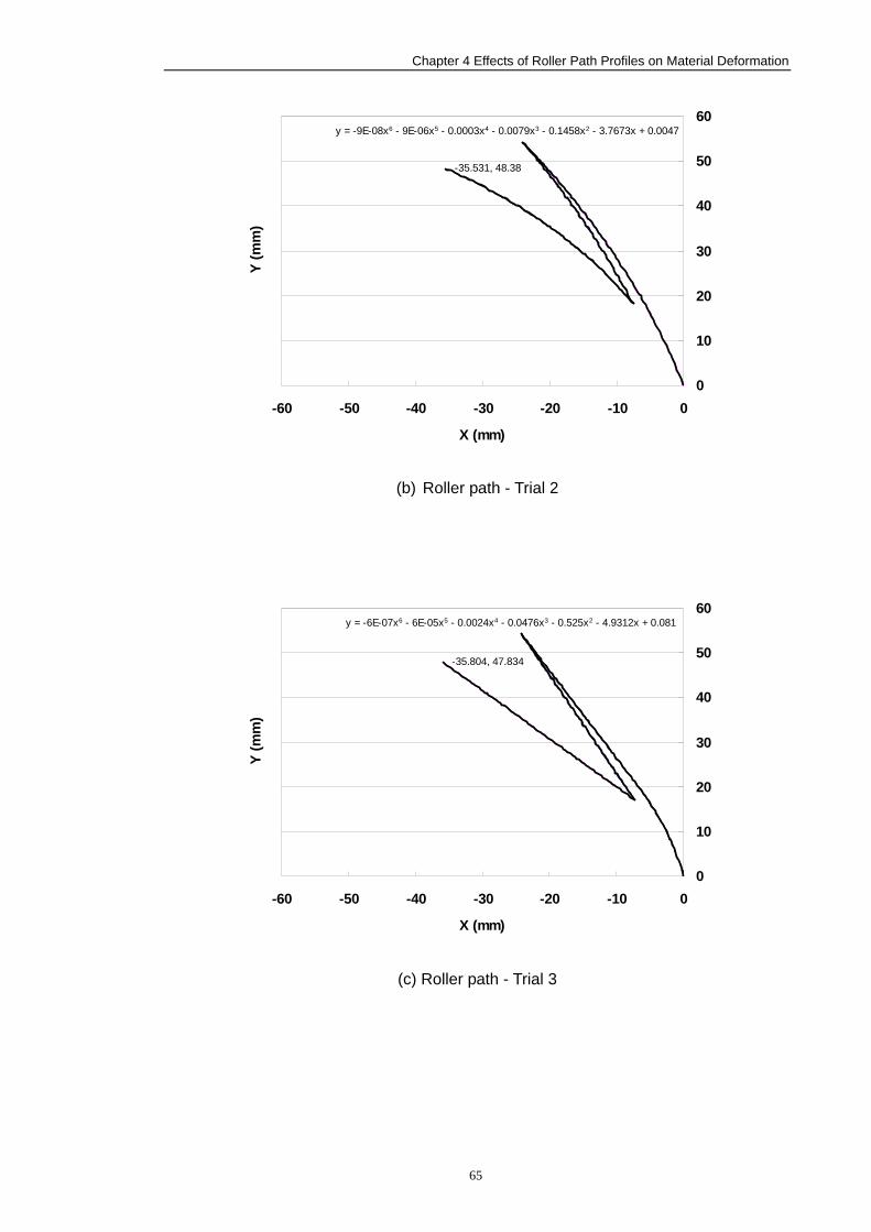
Chapter 4 Effects of Roller Path Profiles on Material Deformation
65
-35.531, 48.38
y = -9E-08x6 - 9E-06x5 - 0.0003x4 - 0.0079x3 - 0.1458x2 - 3.7673x + 0.0047
0
10
20
30
40
50
60
-60 -50 -40 -30 -20 -10 0
X (mm)
Y (m
m)
(b) Roller path - Trial 2
-35.804, 47.834
y = -6E-07x6 - 6E-05x5 - 0.0024x4 - 0.0476x3 - 0.525x2 - 4.9312x + 0.081
0
10
20
30
40
50
60
-60 -50 -40 -30 -20 -10 0
X (mm)
Y (m
m)
(c) Roller path - Trial 3
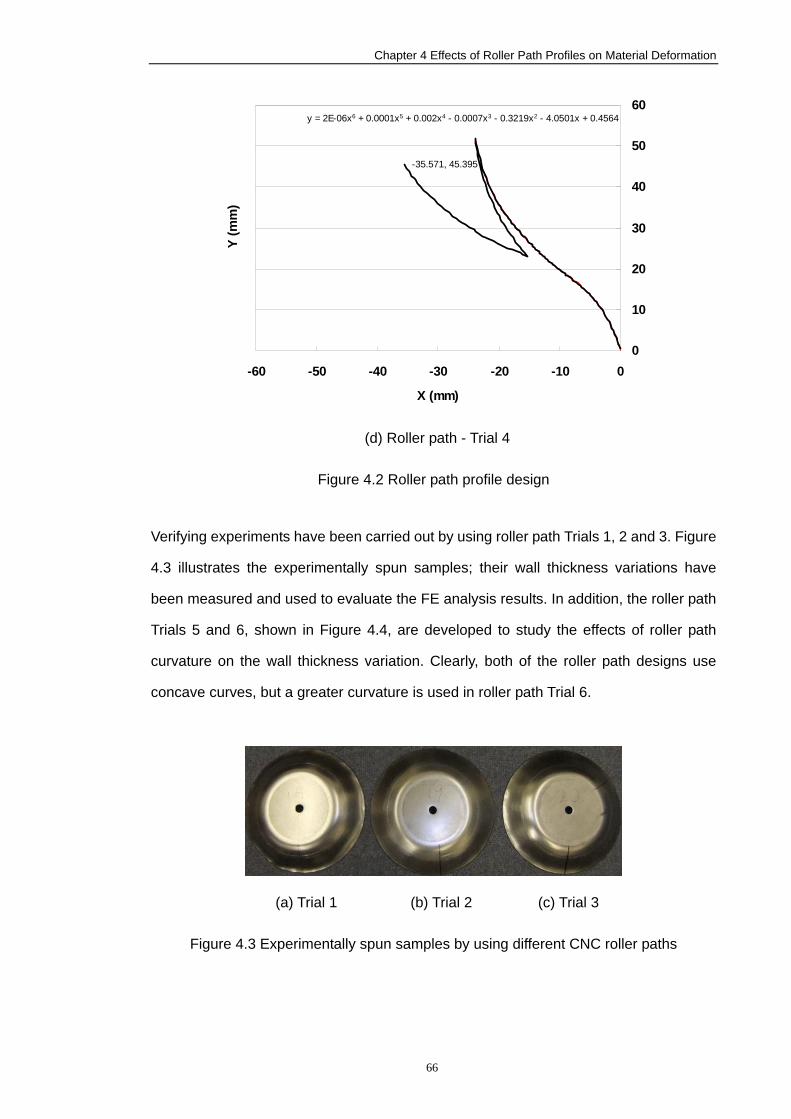
Chapter 4 Effects of Roller Path Profiles on Material Deformation
66
-35.571, 45.395
y = 2E-06x6 + 0.0001x5 + 0.002x4 - 0.0007x3 - 0.3219x2 - 4.0501x + 0.4564
0
10
20
30
40
50
60
-60 -50 -40 -30 -20 -10 0
X (mm)
Y (m
m)
(d) Roller path - Trial 4
Figure 4.2 Roller path profile design
Verifying experiments have been carried out by using roller path Trials 1, 2 and 3. Figure
4.3 illustrates the experimentally spun samples; their wall thickness variations have
been measured and used to evaluate the FE analysis results. In addition, the roller path
Trials 5 and 6, shown in Figure 4.4, are developed to study the effects of roller path
curvature on the wall thickness variation. Clearly, both of the roller path designs use
concave curves, but a greater curvature is used in roller path Trial 6.
(a) Trial 1 (b) Trial 2 (c) Trial 3
Figure 4.3 Experimentally spun samples by using different CNC roller paths
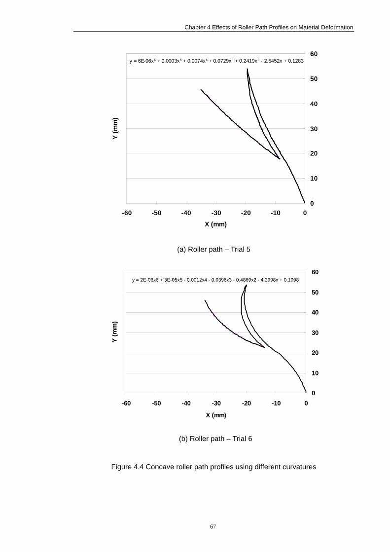
Chapter 4 Effects of Roller Path Profiles on Material Deformation
67
y = 6E-06x6 + 0.0003x5 + 0.0074x4 + 0.0729x3 + 0.2419x2 - 2.5452x + 0.1283
0
10
20
30
40
50
60
-60 -50 -40 -30 -20 -10 0X (mm)
Y (m
m)
(a) Roller path – Trial 5
0
10
20
30
40
50
60
-60 -50 -40 -30 -20 -10 0
X (mm)
Y (m
m)
(b) Roller path – Trial 6
Figure 4.4 Concave roller path profiles using different curvatures
y = 2E-06x6 + 3E-05x5 - 0.0012x4 - 0.0396x3 - 0.4869x2 - 4.2998x + 0.1098
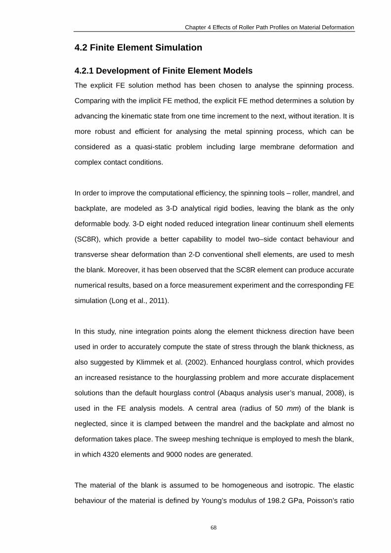
Chapter 4 Effects of Roller Path Profiles on Material Deformation
68
4.2 Finite Element Simulation
4.2.1 Development of Finite Element Models The explicit FE solution method has been chosen to analyse the spinning process.
Comparing with the implicit FE method, the explicit FE method determines a solution by
advancing the kinematic state from one time increment to the next, without iteration. It is
more robust and efficient for analysing the metal spinning process, which can be
considered as a quasi-static problem including large membrane deformation and
complex contact conditions.
In order to improve the computational efficiency, the spinning tools – roller, mandrel, and
backplate, are modeled as 3-D analytical rigid bodies, leaving the blank as the only
deformable body. 3-D eight noded reduced integration linear continuum shell elements
(SC8R), which provide a better capability to model two–side contact behaviour and
transverse shear deformation than 2-D conventional shell elements, are used to mesh
the blank. Moreover, it has been observed that the SC8R element can produce accurate
numerical results, based on a force measurement experiment and the corresponding FE
simulation (Long et al., 2011).
In this study, nine integration points along the element thickness direction have been
used in order to accurately compute the state of stress through the blank thickness, as
also suggested by Klimmek et al. (2002). Enhanced hourglass control, which provides
an increased resistance to the hourglassing problem and more accurate displacement
solutions than the default hourglass control (Abaqus analysis user’s manual, 2008), is
used in the FE analysis models. A central area (radius of 50 mm) of the blank is
neglected, since it is clamped between the mandrel and the backplate and almost no
deformation takes place. The sweep meshing technique is employed to mesh the blank,
in which 4320 elements and 9000 nodes are generated.
The material of the blank is assumed to be homogeneous and isotropic. The elastic
behaviour of the material is defined by Young’s modulus of 198.2 GPa, Poisson’s ratio
Chapter 4 Effects of Roller Path Profiles on Material Deformation
69
of 0.3, and mass density of 7861 kg/m3. The von Mises yielding criterion and isotropic
hardening have been used to model the material plastic response. Figure 4.5 shows the
true stress-strain curve of the material obtained from a uni-axial tensile test, where a flat
sample was tested at room temperature under ASTM E8M (Standard Test Methods for
Tension Testing of Metallic Materials) by Westmoreland Mechanical Testing & Research,
Ltd.
0
50
100
150
200
250
300
350
400
450
0 0.05 0.1 0.15 0.2 0.25 0.3 0.35 0.4
True plastic strain
True
Str
ess
(MPa
)
Figure 4.5 True stress-strain curves of Mild steel (DC01)
The penalty enforcement method and Coulomb’s friction law have been used to
simulate the normal and sliding contact behaviors between the tools and blank,
respectively. The frictional coefficient between the roller and the blank is set to be low,
since the roller rotates along its own axis during the spinning process. Three Coulomb
frictional coefficients have been assigned to three contact pairs of tools and blank:
mandrel-blank 0.2, backplate-blank 0.5, and roller-blank 0.02 (Razavi et al., 2005).
Three steps have been applied in the spinning simulation. At the first step, a
compressive force of 150 kN is applied on the backplate, which accounts for the blank
being clamped between the backplate and mandrel. The second step involves applying
Chapter 4 Effects of Roller Path Profiles on Material Deformation
70
a rotational boundary condition to the backplate and mandrel, in order to model the
synchronous rotation of the blank, backplate and mandrel. Finally, to realise the
complex nonlinear roller path (passes), two displacement boundary conditions in the
local x and z directions, as shown in Figure 4.1(b), are applied to the roller.
These two displacement boundary conditions are calculated by transferring the CNC
programs, which are initially developed in the global coordinate system (X-Y), into the
local coordinates (x-z). The following equations have been used to calculate the local
coordinates from the global coordinates:
θθ cossin YXx −−= (130)
θθ sincos YXz −= (131)
where (x, z) is the local coordinates, (X, Y) represents the global coordinates, andθ is the
angle between axis X and axis z, which is 45° in this experimental setup.
Additionally, to speed-up the FE solution time, the mass scaling method with a scaling
factor of 25 has been used in all of the models. Parallel FE analyses which can
effectively reduce the computing time in the simulation of spinning process (Quigley and
Monaghan, 2002b) have been performed using a workstation of Quad-Core AMD
OpteronTM CPU 2.2GHz and RAM of 6GB.
4.2.2 Verification of Finite Element Models In this section, FE models are verified not only by evaluating mesh convergence and
assessing scaling methods, but also by comparing the FE analysis dimensional results
with experimental measurements.
4.2.2.1 Mesh Convergence Study
A mesh convergence study has been carried out on the FE model using roller path Trial
1. Table 4.1 gives details of the meshes used in the three FE models and the
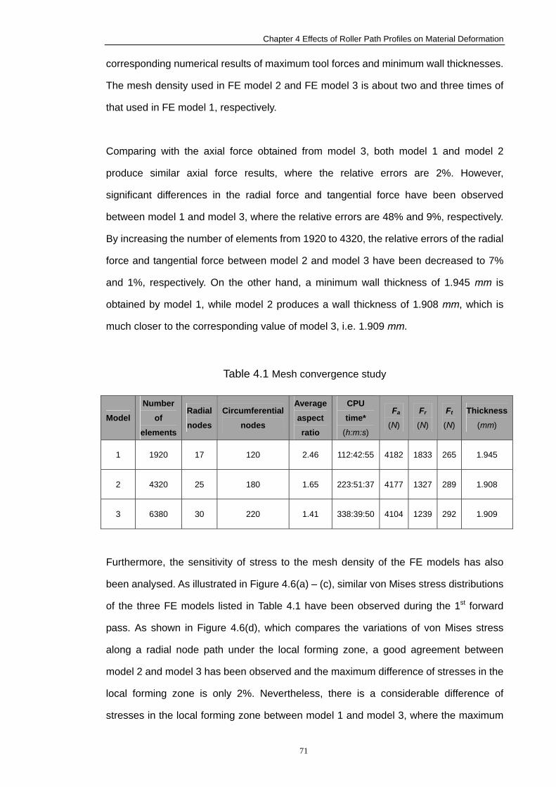
Chapter 4 Effects of Roller Path Profiles on Material Deformation
71
corresponding numerical results of maximum tool forces and minimum wall thicknesses.
The mesh density used in FE model 2 and FE model 3 is about two and three times of
that used in FE model 1, respectively.
Comparing with the axial force obtained from model 3, both model 1 and model 2
produce similar axial force results, where the relative errors are 2%. However,
significant differences in the radial force and tangential force have been observed
between model 1 and model 3, where the relative errors are 48% and 9%, respectively.
By increasing the number of elements from 1920 to 4320, the relative errors of the radial
force and tangential force between model 2 and model 3 have been decreased to 7%
and 1%, respectively. On the other hand, a minimum wall thickness of 1.945 mm is
obtained by model 1, while model 2 produces a wall thickness of 1.908 mm, which is
much closer to the corresponding value of model 3, i.e. 1.909 mm.
Table 4.1 Mesh convergence study
Model
Number
of
elements
Radial
nodes
Circumferential
nodes
Average
aspect
ratio
CPU
time* (h:m:s)
Fa (N)
Fr (N)
Ft (N)
Thickness (mm)
1 1920 17 120 2.46 112:42:55 4182 1833 265 1.945
2 4320 25 180 1.65 223:51:37 4177 1327 289 1.908
3 6380 30 220 1.41 338:39:50 4104 1239 292 1.909
Furthermore, the sensitivity of stress to the mesh density of the FE models has also
been analysed. As illustrated in Figure 4.6(a) – (c), similar von Mises stress distributions
of the three FE models listed in Table 4.1 have been observed during the 1st forward
pass. As shown in Figure 4.6(d), which compares the variations of von Mises stress
along a radial node path under the local forming zone, a good agreement between
model 2 and model 3 has been observed and the maximum difference of stresses in the
local forming zone is only 2%. Nevertheless, there is a considerable difference of
stresses in the local forming zone between model 1 and model 3, where the maximum
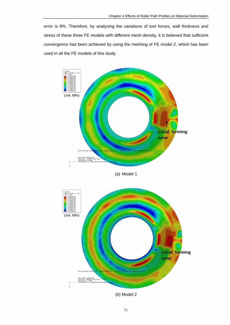
Chapter 4 Effects of Roller Path Profiles on Material Deformation
72
error is 9%. Therefore, by analysing the variations of tool forces, wall thickness and
stress of these three FE models with different mesh density, it is believed that sufficient
convergence has been achieved by using the meshing of FE model 2, which has been
used in all the FE models of this study.
(a) Model 1
(b) Model 2
Local forming zone
Local forming zone
Unit: MPa
Unit: MPa
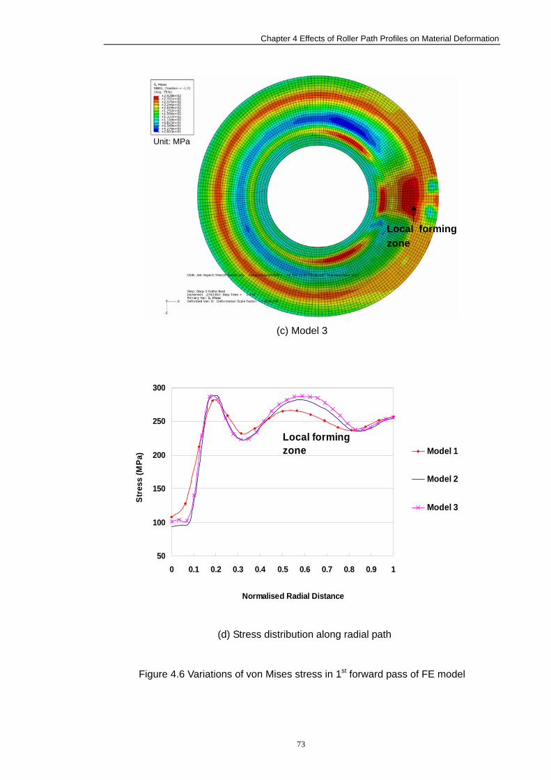
Chapter 4 Effects of Roller Path Profiles on Material Deformation
73
(c) Model 3
50
100
150
200
250
300
0 0.1 0.2 0.3 0.4 0.5 0.6 0.7 0.8 0.9 1
Normalised Radial Distance
Stre
ss (M
Pa) Model 1
Model 2
Model 3
Local formingzone
(d) Stress distribution along radial path
Figure 4.6 Variations of von Mises stress in 1st forward pass of FE model
Local forming zone
Unit: MPa
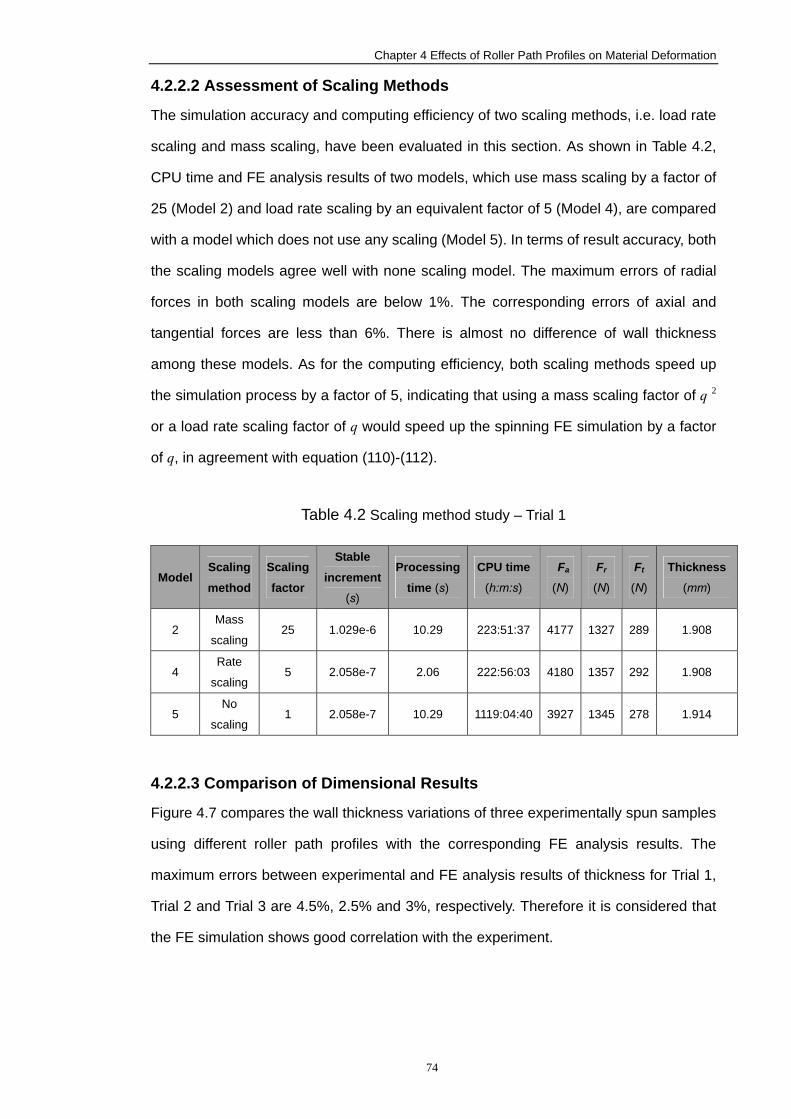
Chapter 4 Effects of Roller Path Profiles on Material Deformation
74
4.2.2.2 Assessment of Scaling Methods
The simulation accuracy and computing efficiency of two scaling methods, i.e. load rate
scaling and mass scaling, have been evaluated in this section. As shown in Table 4.2,
CPU time and FE analysis results of two models, which use mass scaling by a factor of
25 (Model 2) and load rate scaling by an equivalent factor of 5 (Model 4), are compared
with a model which does not use any scaling (Model 5). In terms of result accuracy, both
the scaling models agree well with none scaling model. The maximum errors of radial
forces in both scaling models are below 1%. The corresponding errors of axial and
tangential forces are less than 6%. There is almost no difference of wall thickness
among these models. As for the computing efficiency, both scaling methods speed up
the simulation process by a factor of 5, indicating that using a mass scaling factor of q 2
or a load rate scaling factor of q would speed up the spinning FE simulation by a factor
of q, in agreement with equation (110)-(112).
Table 4.2 Scaling method study – Trial 1
Model Scaling
method
Scaling
factor
Stable
increment (s)
Processing
time (s)
CPU time(h:m:s)
Fa (N)
Fr (N)
Ft (N)
Thickness (mm)
2 Mass
scaling 25 1.029e-6 10.29 223:51:37 4177 1327 289 1.908
4 Rate
scaling 5 2.058e-7 2.06 222:56:03 4180 1357 292 1.908
5 No
scaling 1 2.058e-7 10.29 1119:04:40 3927 1345 278 1.914
4.2.2.3 Comparison of Dimensional Results
Figure 4.7 compares the wall thickness variations of three experimentally spun samples
using different roller path profiles with the corresponding FE analysis results. The
maximum errors between experimental and FE analysis results of thickness for Trial 1,
Trial 2 and Trial 3 are 4.5%, 2.5% and 3%, respectively. Therefore it is considered that
the FE simulation shows good correlation with the experiment.
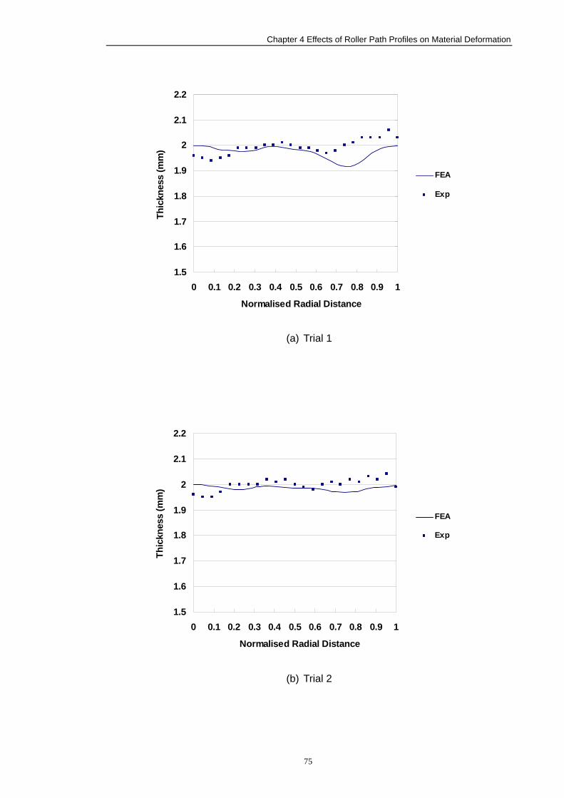
Chapter 4 Effects of Roller Path Profiles on Material Deformation
75
1.5
1.6
1.7
1.8
1.9
2
2.1
2.2
0 0.1 0.2 0.3 0.4 0.5 0.6 0.7 0.8 0.9 1
Normalised Radial Distance
Thic
knes
s (m
m)
FEA
Exp
(a) Trial 1
1.5
1.6
1.7
1.8
1.9
2
2.1
2.2
0 0.1 0.2 0.3 0.4 0.5 0.6 0.7 0.8 0.9 1
Normalised Radial Distance
Thic
knes
s (m
m)
FEA
Exp
(b) Trial 2
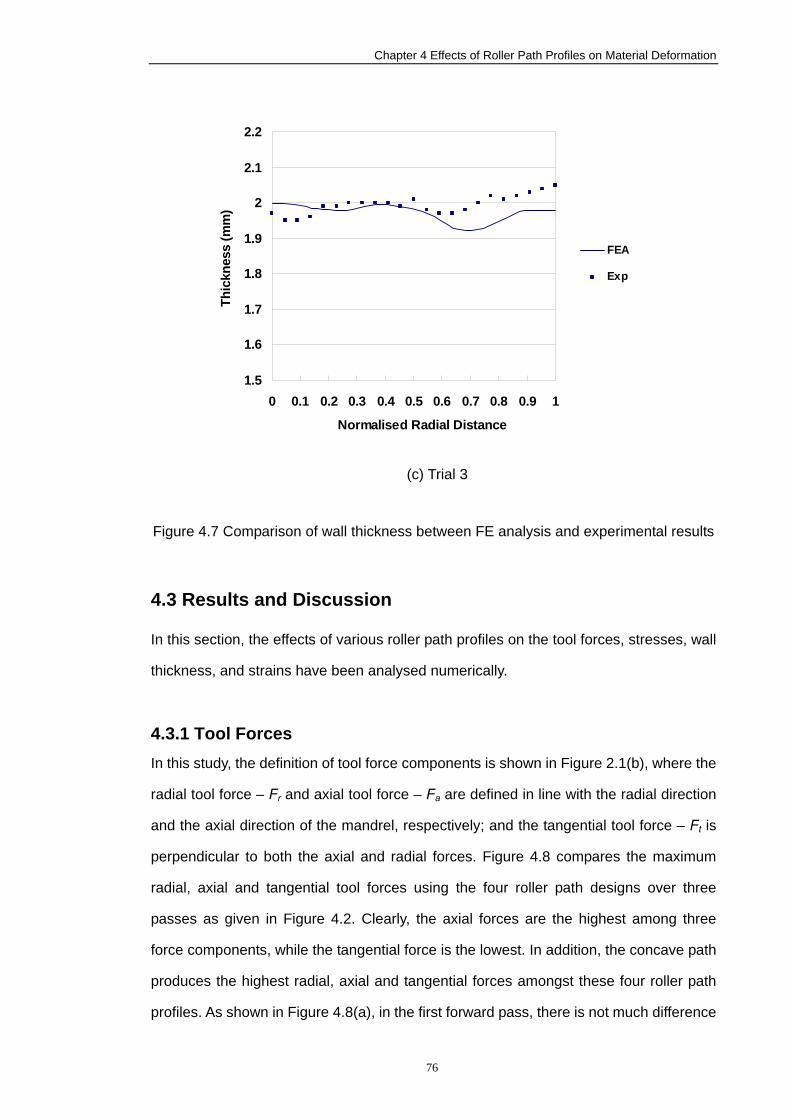
Chapter 4 Effects of Roller Path Profiles on Material Deformation
76
1.5
1.6
1.7
1.8
1.9
2
2.1
2.2
0 0.1 0.2 0.3 0.4 0.5 0.6 0.7 0.8 0.9 1
Normalised Radial Distance
Thic
knes
s (m
m)
FEA
Exp
(c) Trial 3
Figure 4.7 Comparison of wall thickness between FE analysis and experimental results
4.3 Results and Discussion
In this section, the effects of various roller path profiles on the tool forces, stresses, wall
thickness, and strains have been analysed numerically.
4.3.1 Tool Forces In this study, the definition of tool force components is shown in Figure 2.1(b), where the
radial tool force – Fr and axial tool force – Fa are defined in line with the radial direction
and the axial direction of the mandrel, respectively; and the tangential tool force – Ft is
perpendicular to both the axial and radial forces. Figure 4.8 compares the maximum
radial, axial and tangential tool forces using the four roller path designs over three
passes as given in Figure 4.2. Clearly, the axial forces are the highest among three
force components, while the tangential force is the lowest. In addition, the concave path
produces the highest radial, axial and tangential forces amongst these four roller path
profiles. As shown in Figure 4.8(a), in the first forward pass, there is not much difference
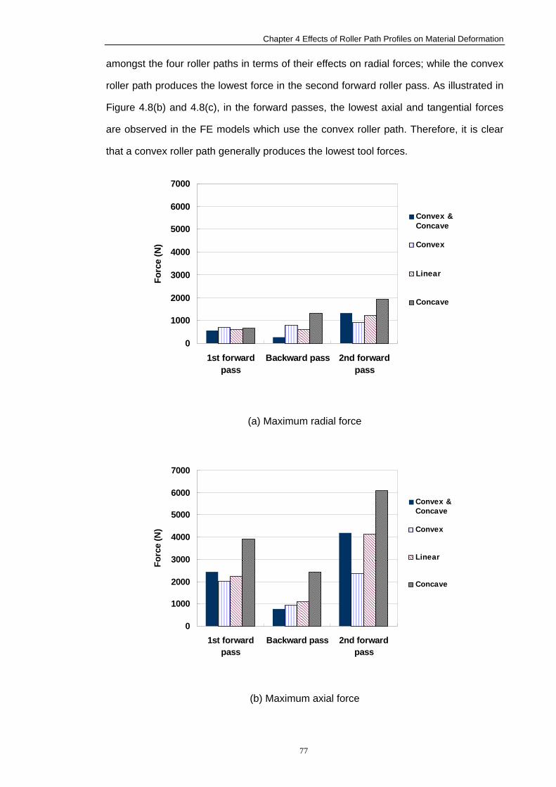
Chapter 4 Effects of Roller Path Profiles on Material Deformation
77
amongst the four roller paths in terms of their effects on radial forces; while the convex
roller path produces the lowest force in the second forward roller pass. As illustrated in
Figure 4.8(b) and 4.8(c), in the forward passes, the lowest axial and tangential forces
are observed in the FE models which use the convex roller path. Therefore, it is clear
that a convex roller path generally produces the lowest tool forces.
0
1000
2000
3000
4000
5000
6000
7000
1st forwardpass
Backward pass 2nd forwardpass
Forc
e (N
)
Convex &Concave
Convex
Linear
Concave
(a) Maximum radial force
0
1000
2000
3000
4000
5000
6000
7000
1st forwardpass
Backward pass 2nd forwardpass
Forc
e (N
)
Convex &Concave
Convex
Linear
Concave
(b) Maximum axial force
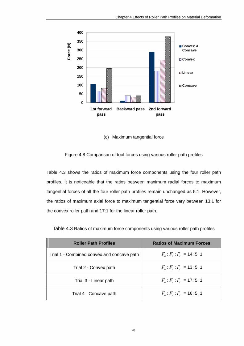
Chapter 4 Effects of Roller Path Profiles on Material Deformation
78
0
50
100
150
200
250
300
350
400
1st forwardpass
Backward pass 2nd forwardpass
Forc
e (N
)
Convex &Concave
Convex
Linear
Concave
(c) Maximum tangential force
Figure 4.8 Comparison of tool forces using various roller path profiles
Table 4.3 shows the ratios of maximum force components using the four roller path
profiles. It is noticeable that the ratios between maximum radial forces to maximum
tangential forces of all the four roller path profiles remain unchanged as 5:1. However,
the ratios of maximum axial force to maximum tangential force vary between 13:1 for
the convex roller path and 17:1 for the linear roller path.
Table 4.3 Ratios of maximum force components using various roller path profiles
Roller Path Profiles Ratios of Maximum Forces
Trial 1 - Combined convex and concave path tra FFF :: = 14: 5: 1
Trial 2 - Convex path tra FFF :: = 13: 5: 1
Trial 3 - Linear path tra FFF :: = 17: 5: 1
Trial 4 - Concave path tra FFF :: = 16: 5: 1
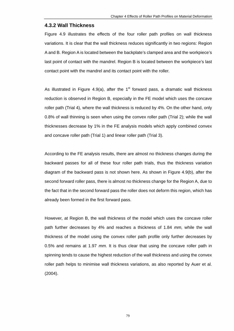
Chapter 4 Effects of Roller Path Profiles on Material Deformation
79
4.3.2 Wall Thickness Figure 4.9 illustrates the effects of the four roller path profiles on wall thickness
variations. It is clear that the wall thickness reduces significantly in two regions: Region
A and B. Region A is located between the backplate’s clamped area and the workpiece’s
last point of contact with the mandrel. Region B is located between the workpiece’s last
contact point with the mandrel and its contact point with the roller.
As illustrated in Figure 4.9(a), after the 1st forward pass, a dramatic wall thickness
reduction is observed in Region B, especially in the FE model which uses the concave
roller path (Trial 4), where the wall thickness is reduced by 4%. On the other hand, only
0.8% of wall thinning is seen when using the convex roller path (Trial 2); while the wall
thicknesses decrease by 1% in the FE analysis models which apply combined convex
and concave roller path (Trial 1) and linear roller path (Trial 3).
According to the FE analysis results, there are almost no thickness changes during the
backward passes for all of these four roller path trials, thus the thickness variation
diagram of the backward pass is not shown here. As shown in Figure 4.9(b), after the
second forward roller pass, there is almost no thickness change for the Region A, due to
the fact that in the second forward pass the roller does not deform this region, which has
already been formed in the first forward pass.
However, at Region B, the wall thickness of the model which uses the concave roller
path further decreases by 4% and reaches a thickness of 1.84 mm, while the wall
thickness of the model using the convex roller path profile only further decreases by
0.5% and remains at 1.97 mm. It is thus clear that using the concave roller path in
spinning tends to cause the highest reduction of the wall thickness and using the convex
roller path helps to minimise wall thickness variations, as also reported by Auer et al.
(2004).
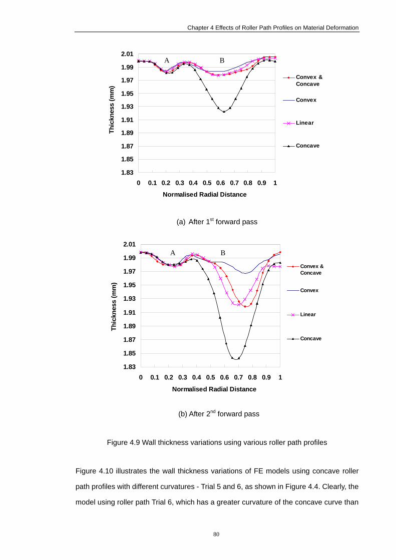
Chapter 4 Effects of Roller Path Profiles on Material Deformation
80
1.83
1.85
1.87
1.89
1.91
1.93
1.95
1.97
1.99
2.01
0 0.1 0.2 0.3 0.4 0.5 0.6 0.7 0.8 0.9 1
Normalised Radial Distance
Thic
knes
s (m
m)
Convex &Concave
Convex
Linear
Concave
(a) After 1st forward pass
1.83
1.85
1.87
1.89
1.91
1.93
1.95
1.97
1.99
2.01
0 0.1 0.2 0.3 0.4 0.5 0.6 0.7 0.8 0.9 1
Normalised Radial Distance
Thic
knes
s (m
m)
Convex &Concave
Convex
Linear
Concave
(b) After 2nd forward pass
Figure 4.9 Wall thickness variations using various roller path profiles
Figure 4.10 illustrates the wall thickness variations of FE models using concave roller
path profiles with different curvatures - Trial 5 and 6, as shown in Figure 4.4. Clearly, the
model using roller path Trial 6, which has a greater curvature of the concave curve than
A B
A B
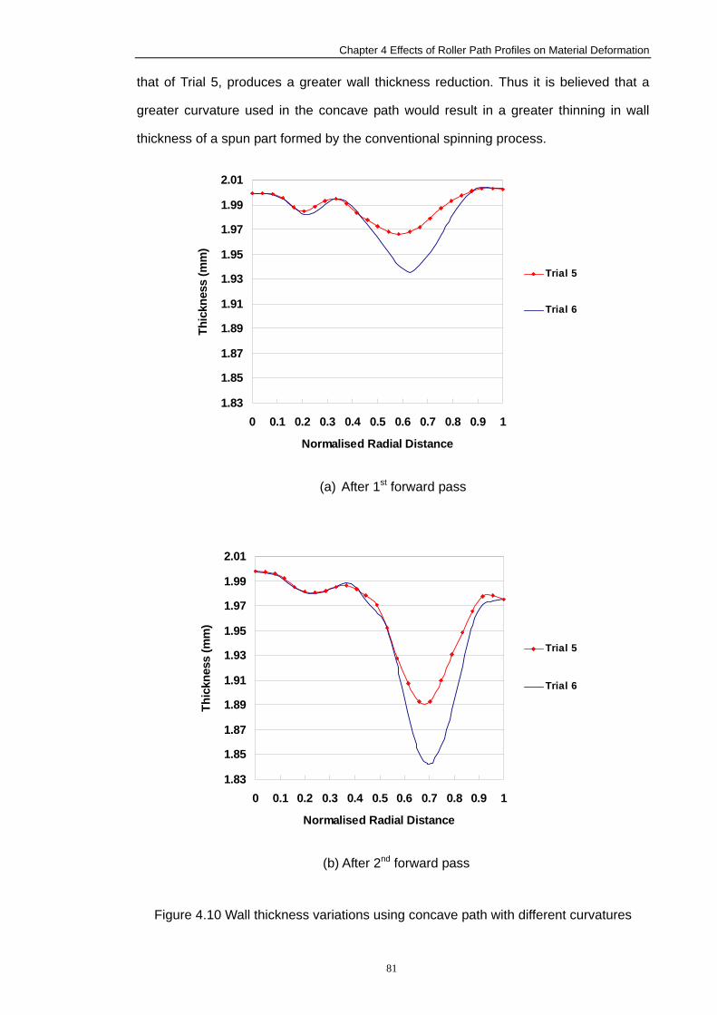
Chapter 4 Effects of Roller Path Profiles on Material Deformation
81
that of Trial 5, produces a greater wall thickness reduction. Thus it is believed that a
greater curvature used in the concave path would result in a greater thinning in wall
thickness of a spun part formed by the conventional spinning process.
1.83
1.85
1.87
1.89
1.91
1.93
1.95
1.97
1.99
2.01
0 0.1 0.2 0.3 0.4 0.5 0.6 0.7 0.8 0.9 1
Normalised Radial Distance
Thic
knes
s (m
m)
Trial 5
Trial 6
(a) After 1st forward pass
1.83
1.85
1.87
1.89
1.91
1.93
1.95
1.97
1.99
2.01
0 0.1 0.2 0.3 0.4 0.5 0.6 0.7 0.8 0.9 1
Normalised Radial Distance
Thic
knes
s (m
m)
Trial 5
Trial 6
(b) After 2nd forward pass
Figure 4.10 Wall thickness variations using concave path with different curvatures
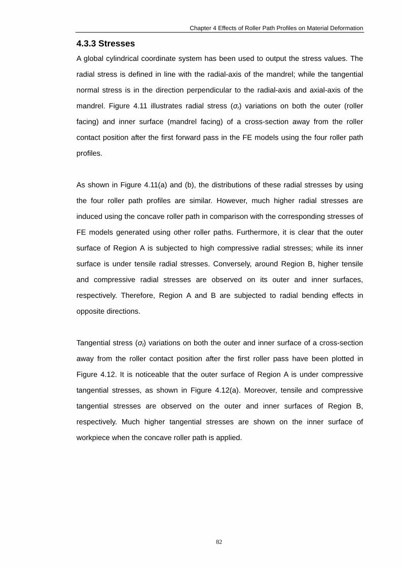
Chapter 4 Effects of Roller Path Profiles on Material Deformation
82
4.3.3 Stresses A global cylindrical coordinate system has been used to output the stress values. The
radial stress is defined in line with the radial-axis of the mandrel; while the tangential
normal stress is in the direction perpendicular to the radial-axis and axial-axis of the
mandrel. Figure 4.11 illustrates radial stress (σr) variations on both the outer (roller
facing) and inner surface (mandrel facing) of a cross-section away from the roller
contact position after the first forward pass in the FE models using the four roller path
profiles.
As shown in Figure 4.11(a) and (b), the distributions of these radial stresses by using
the four roller path profiles are similar. However, much higher radial stresses are
induced using the concave roller path in comparison with the corresponding stresses of
FE models generated using other roller paths. Furthermore, it is clear that the outer
surface of Region A is subjected to high compressive radial stresses; while its inner
surface is under tensile radial stresses. Conversely, around Region B, higher tensile
and compressive radial stresses are observed on its outer and inner surfaces,
respectively. Therefore, Region A and B are subjected to radial bending effects in
opposite directions.
Tangential stress (σt) variations on both the outer and inner surface of a cross-section
away from the roller contact position after the first roller pass have been plotted in
Figure 4.12. It is noticeable that the outer surface of Region A is under compressive
tangential stresses, as shown in Figure 4.12(a). Moreover, tensile and compressive
tangential stresses are observed on the outer and inner surfaces of Region B,
respectively. Much higher tangential stresses are shown on the inner surface of
workpiece when the concave roller path is applied.
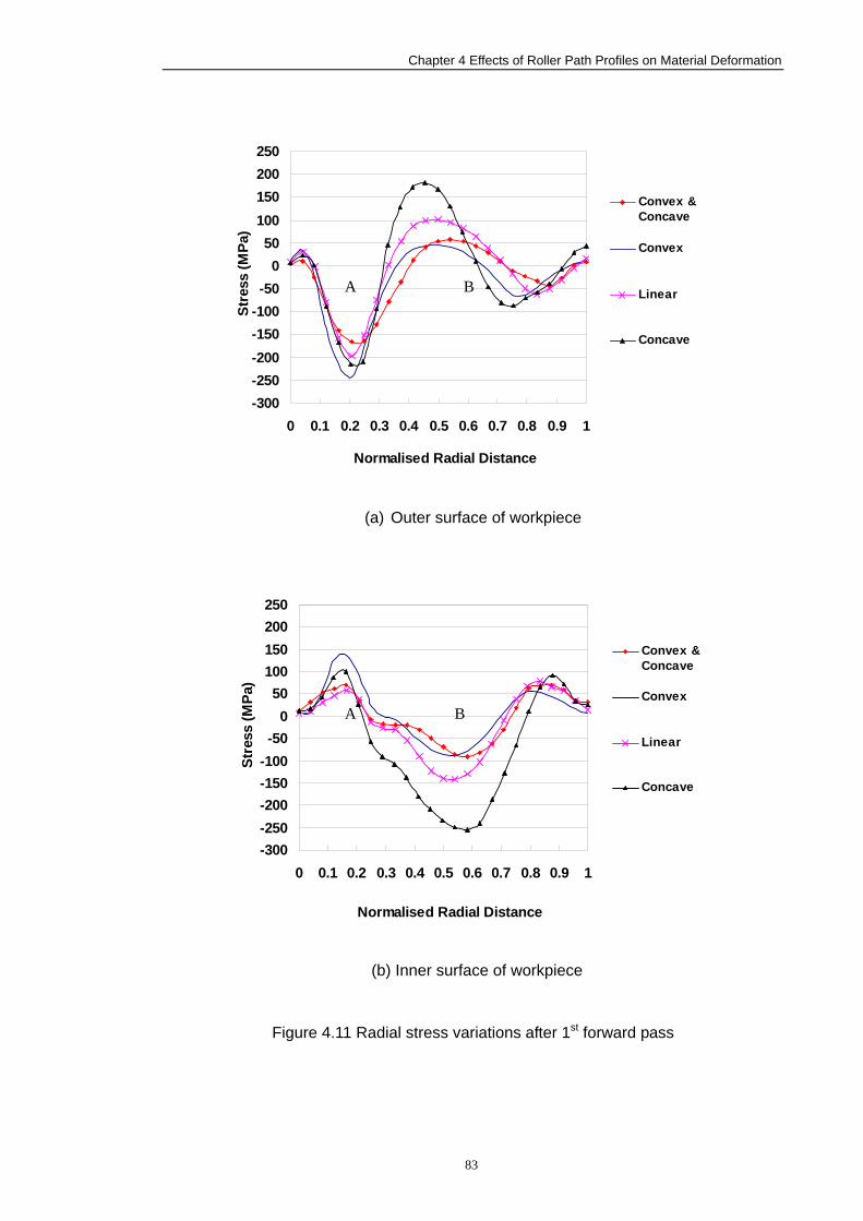
Chapter 4 Effects of Roller Path Profiles on Material Deformation
83
-300-250-200-150-100-50
050
100150200250
0 0.1 0.2 0.3 0.4 0.5 0.6 0.7 0.8 0.9 1
Normalised Radial Distance
Stre
ss (M
Pa)
Convex &Concave
Convex
Linear
Concave
(a) Outer surface of workpiece
-300-250-200-150-100-50
050
100150200250
0 0.1 0.2 0.3 0.4 0.5 0.6 0.7 0.8 0.9 1
Normalised Radial Distance
Stre
ss (M
Pa)
Convex &Concave
Convex
Linear
Concave
(b) Inner surface of workpiece
Figure 4.11 Radial stress variations after 1st forward pass
A B
A B
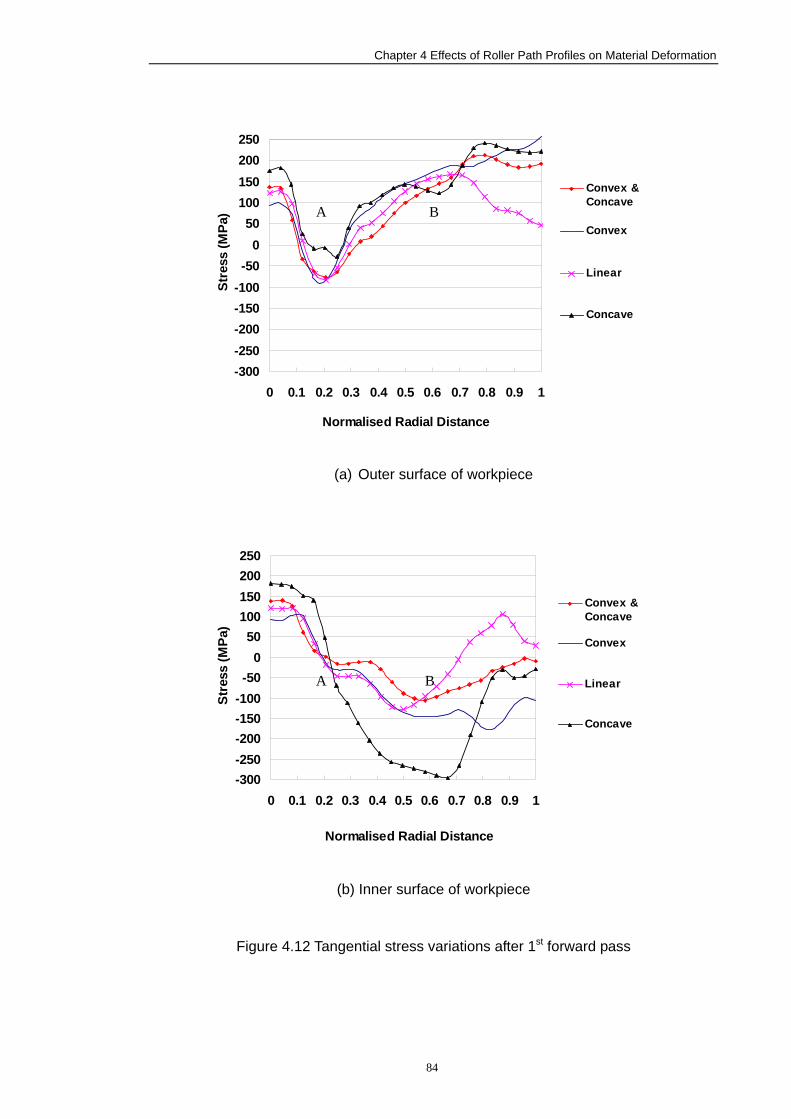
Chapter 4 Effects of Roller Path Profiles on Material Deformation
84
-300-250-200-150-100-50
050
100150200250
0 0.1 0.2 0.3 0.4 0.5 0.6 0.7 0.8 0.9 1
Normalised Radial Distance
Stre
ss (M
Pa)
Convex &Concave
Convex
Linear
Concave
(a) Outer surface of workpiece
-300-250-200-150-100-50
050
100150200250
0 0.1 0.2 0.3 0.4 0.5 0.6 0.7 0.8 0.9 1
Normalised Radial Distance
Stre
ss (M
Pa)
Convex &Concave
Convex
Linear
Concave
(b) Inner surface of workpiece
Figure 4.12 Tangential stress variations after 1st forward pass
A B
A B
Chapter 4 Effects of Roller Path Profiles on Material Deformation
85
4.3.4 Strains In order to analyse the cause of wall thinning in the conventional spinning process,
variations of the maximum in-plane principal strain (radial strain) and minimum in-plane
principal strain (tangential strain) after the first forward pass have been plotted in Figure
4.13 and 4.14, respectively. As shown in Figure 4.13(a), high tensile radial strains are
observed in both Region A and B in the outer surface of workpiece; whilst in the inner
surface high tensile radial strains take place mainly around Region B, as demonstrated
in Figure 4.13(b). These high in-plane tensile radial strains are believed to be the reason
of the significant wall thinning in Regions A and B shown in Figure 4.9. In addition, the
FE model which uses a concave roller path profile produces much higher tensile radial
strains in Region B than FE models which use other roller path profiles, resulting in a
higher amount of wall thinning when the concave roller path is applied.
As shown in Figure 4.14, except for Region A in the outer surface of the workpece, both
the inner and outer surfaces are subjected to in-plane compressive tangential strains,
which would lead to a certain degree of compensation to the wall thinning. However, the
dominant high in-plane tensile radial strains shown in Figure 4.13 play a decisive role in
wall thinning. It is also noticeable that unlike the variations of in-plane radial strains
amongst the models using various roller path profiles, there is not much difference of
in-plane tangential strains.
Figure 4.15(a) illustrates the variations of out-of-plane principal strain (thickness strain)
in the outer surface of the workpiece. It is clear that both Region A and B of the outer
surface are subjected to high compressive thickness strains, indicating the decreasing
of wall thickness in those regions. The variations of the thickness strain in the inner
surface of the workpiece have been plotted in Figure 4.15(b). In Region A of the inner
surface, the low tensile thickness strain is cancelled out by the relatively high
compressive thickness strain of the outer surface. Conversely, the compressive
thickness strain in the inner surface of Region B is enhanced by the compressive
thickness strain of its outer surface. These combined effects of the strains result in less
wall thinning in Region A than Region B, as shown in Figure 4.9.
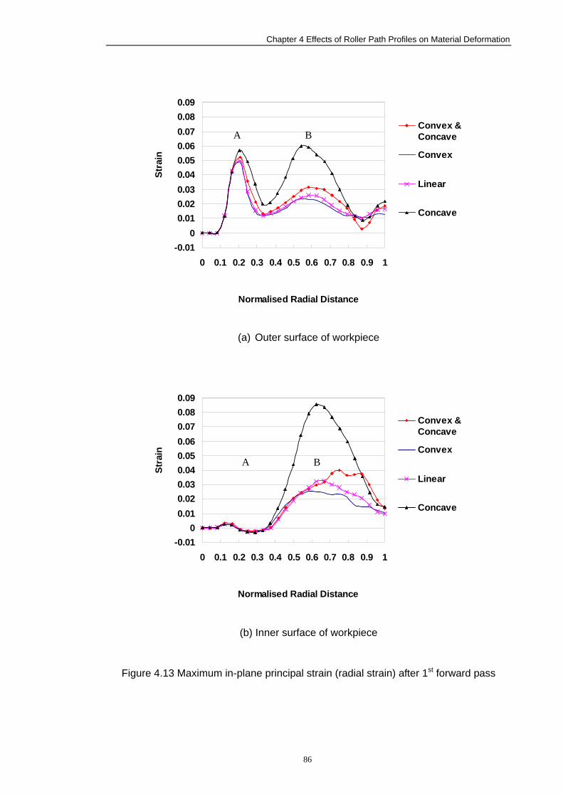
Chapter 4 Effects of Roller Path Profiles on Material Deformation
86
-0.010
0.010.020.030.040.050.060.070.080.09
0 0.1 0.2 0.3 0.4 0.5 0.6 0.7 0.8 0.9 1
Normalised Radial Distance
Stra
in
Convex &Concave
Convex
Linear
Concave
(a) Outer surface of workpiece
-0.010
0.010.020.030.040.050.060.070.080.09
0 0.1 0.2 0.3 0.4 0.5 0.6 0.7 0.8 0.9 1
Normalised Radial Distance
Stra
in
Convex &Concave
Convex
Linear
Concave
(b) Inner surface of workpiece
Figure 4.13 Maximum in-plane principal strain (radial strain) after 1st forward pass
A B
A B
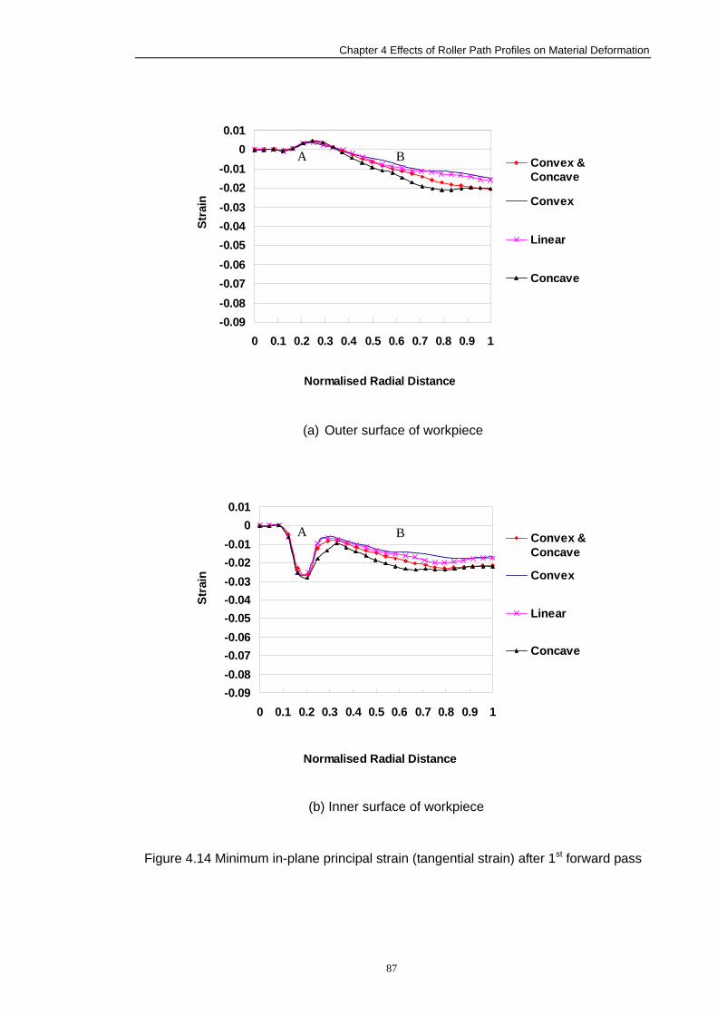
Chapter 4 Effects of Roller Path Profiles on Material Deformation
87
-0.09-0.08-0.07-0.06-0.05-0.04-0.03-0.02-0.01
00.01
0 0.1 0.2 0.3 0.4 0.5 0.6 0.7 0.8 0.9 1
Normalised Radial Distance
Stra
in
Convex &Concave
Convex
Linear
Concave
(a) Outer surface of workpiece
-0.09-0.08-0.07-0.06-0.05-0.04-0.03-0.02-0.01
00.01
0 0.1 0.2 0.3 0.4 0.5 0.6 0.7 0.8 0.9 1
Normalised Radial Distance
Stra
in
Convex &Concave
Convex
Linear
Concave
(b) Inner surface of workpiece
Figure 4.14 Minimum in-plane principal strain (tangential strain) after 1st forward pass
A B
A B
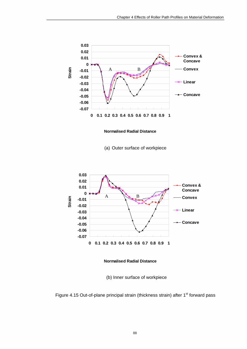
Chapter 4 Effects of Roller Path Profiles on Material Deformation
88
-0.07-0.06-0.05-0.04-0.03-0.02-0.01
00.010.020.03
0 0.1 0.2 0.3 0.4 0.5 0.6 0.7 0.8 0.9 1
Normalised Radial Distance
Stra
in
Convex &Concave
Convex
Linear
Concave
(a) Outer surface of workpiece
-0.07-0.06-0.05-0.04-0.03-0.02-0.01
00.010.020.03
0 0.1 0.2 0.3 0.4 0.5 0.6 0.7 0.8 0.9 1
Normalised Radial Distance
Stra
in
Convex &Concave
Convex
Linear
Concave
(b) Inner surface of workpiece
Figure 4.15 Out-of-plane principal strain (thickness strain) after 1st forward pass
A B
A B
Chapter 4 Effects of Roller Path Profiles on Material Deformation
89
4.4 Summary and Conclusion
In this chapter, four different roller path profiles, i.e. combined concave and convex,
convex, linear and concave curves, have been designed by using spinning CAM
software - OPUS. The 3-D elastic-plastic FE models of metal spinning are developed by
using FE software - Abaqus. The FE models have been verified by carrying out mesh
convergence study, assessing scaling methods, and also by comparing the dimensional
results. Based on the experimental investigation and FE analysis of the conventional
spinning process using the various roller path profiles, the following conclusions may be
drawn:
a) Both mass scaling and load scaling methods are able to significantly speed up the
FE simulation of a conventional spinning process. Using a mass scaling factor of f 2
or a load rate scaling factor of f would speed up the spinning FE simulation by a
factor of f.
b) FE analysis results indicate that the concave roller path produces the highest tool
forces amongst the four different roller path designs. The lowest tool forces are
generally observed when the convex roller path is used.
c) Using the concave roller path tends to cause the highest reduction of the wall
thickness of the spun part, while the convex roller path helps to maintain the
original wall thickness. A greater curvature of the concave path would result in a
higher amount of wall thinning of the spun part.
d) High tensile radial strains and low compressive tangential strains have been
observed in the FE models. In addition, if a concave roller path is applied, much
higher tensile radial strains would be obtained, resulting in greater wall thinning.
e) Two pairs of oppositely directed radial bending effects have been observed in the
workpiece during the conventional spinning process.
Chapter 5 Analysis of Material Deformation in Multi-pass Conventional Spinning
90
5. Analysis of Material Deformation in Multi-pass
Conventional Spinning
In the current academic research, most published papers on conventional spinning are
based on mandrels with a simple linear profile, e.g. conical and cylindrical shapes.
Investigations on spinning are mainly limited to no more than three passes (mainly a
linear path). Nevertheless, in the industry application, a considerable amount of roller
passes have to be used in order to successfully spin a complicated product. Therefore,
it is essential to develop a method of generating multiple roller passes for a mandrel with
a nonlinear profile and to investigate the material deformation in the multi-pass spinning
process. In this chapter, to make the workpiece conform to the non-linear profile of a
mandrel, the tool compensation technique has been proposed and employed in the
CNC multiple roller passes design. The Taguchi method is used to design the
experimental runs and analyse the effects of three process parameters on the
dimensional variations of the spun parts. Furthermore, FE simulation is conducted to
investigate the variations of tool forces, stresses, wall thickness and strains in this
multi-pass spinning process.
5.1 Experimental Investigation
Based on the same experimental setup of Chapter 4, i.e. Figure 4.1, multiple roller
passes which can successfully complete the spun part are developed and used to
conduct the experiment. The blanks are again made of mild steel (DC01) with diameter
of 240 mm and thickness of 2 mm. In this section, the methodologies of tool
compensation and Taguchi experimental design are discussed.
5.1.1 Tool Compensation in CNC Programming To make the workpiece conform to the nonlinear profile of the mandrel, tool
compensation has to be taken into account in the process of designing multiple roller
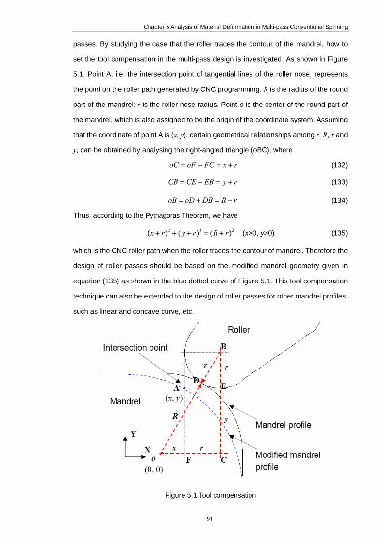
Chapter 5 Analysis of Material Deformation in Multi-pass Conventional Spinning
91
passes. By studying the case that the roller traces the contour of the mandrel, how to
set the tool compensation in the multi-pass design is investigated. As shown in Figure
5.1, Point A, i.e. the intersection point of tangential lines of the roller nose, represents
the point on the roller path generated by CNC programming. R is the radius of the round
part of the mandrel; r is the roller nose radius. Point o is the center of the round part of
the mandrel, which is also assigned to be the origin of the coordinate system. Assuming
that the coordinate of point A is (x, y), certain geometrical relationships among r, R, x and
y, can be obtained by analysing the right-angled triangle (oBC), where
rxFCoFoC +=+= (132)
ryEBCECB +=+= (133)
rRDBoDoB +=+= (134)
Thus, according to the Pythagoras Theorem, we have
222 )()()( rRryrx +=+++ (x>0, y>0) (135)
which is the CNC roller path when the roller traces the contour of mandrel. Therefore the
design of roller passes should be based on the modified mandrel geometry given in
equation (135) as shown in the blue dotted curve of Figure 5.1. This tool compensation
technique can also be extended to the design of roller passes for other mandrel profiles,
such as linear and concave curve, etc.
Figure 5.1 Tool compensation
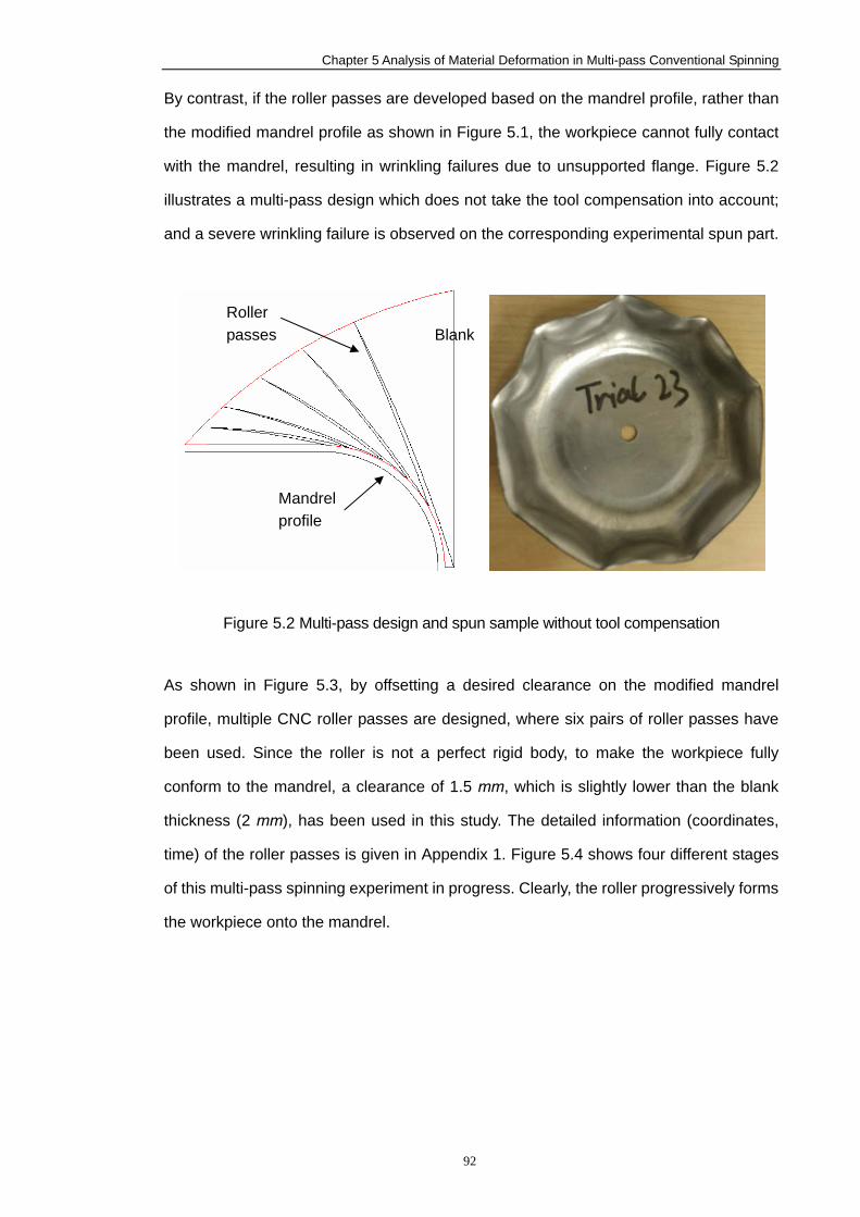
Chapter 5 Analysis of Material Deformation in Multi-pass Conventional Spinning
92
By contrast, if the roller passes are developed based on the mandrel profile, rather than
the modified mandrel profile as shown in Figure 5.1, the workpiece cannot fully contact
with the mandrel, resulting in wrinkling failures due to unsupported flange. Figure 5.2
illustrates a multi-pass design which does not take the tool compensation into account;
and a severe wrinkling failure is observed on the corresponding experimental spun part.
Figure 5.2 Multi-pass design and spun sample without tool compensation
As shown in Figure 5.3, by offsetting a desired clearance on the modified mandrel
profile, multiple CNC roller passes are designed, where six pairs of roller passes have
been used. Since the roller is not a perfect rigid body, to make the workpiece fully
conform to the mandrel, a clearance of 1.5 mm, which is slightly lower than the blank
thickness (2 mm), has been used in this study. The detailed information (coordinates,
time) of the roller passes is given in Appendix 1. Figure 5.4 shows four different stages
of this multi-pass spinning experiment in progress. Clearly, the roller progressively forms
the workpiece onto the mandrel.
Roller passes
Mandrel profile
Blank
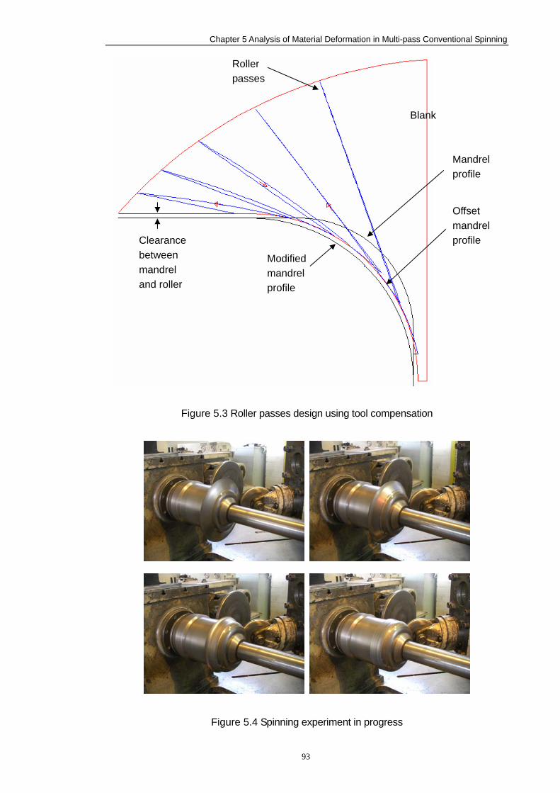
Chapter 5 Analysis of Material Deformation in Multi-pass Conventional Spinning
93
Figure 5.3 Roller passes design using tool compensation
Figure 5.4 Spinning experiment in progress
Modified mandrel profile
Mandrel profile
Blank
Roller passes
Clearance between mandrel and roller
Offset mandrel profile
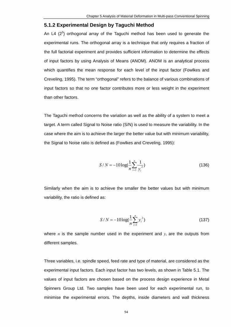
Chapter 5 Analysis of Material Deformation in Multi-pass Conventional Spinning
94
5.1.2 Experimental Design by Taguchi Method An L4 (23) orthogonal array of the Taguchi method has been used to generate the
experimental runs. The orthogonal array is a technique that only requires a fraction of
the full factorial experiment and provides sufficient information to determine the effects
of input factors by using Analysis of Means (ANOM). ANOM is an analytical process
which quantifies the mean response for each level of the input factor (Fowlkes and
Creveling, 1995). The term “orthogonal” refers to the balance of various combinations of
input factors so that no one factor contributes more or less weight in the experiment
than other factors.
The Taguchi method concerns the variation as well as the ability of a system to meet a
target. A term called Signal to Noise ratio (S/N) is used to measure the variability. In the
case where the aim is to achieve the larger the better value but with minimum variability,
the Signal to Noise ratio is defined as (Fowlkes and Creveling, 1995):
∑=
−=n
i iynNS
12 )11log(10/ (136)
Similarly when the aim is to achieve the smaller the better values but with minimum
variability, the ratio is defined as:
∑=
−=n
iiy
nNS
1
2 )1log(10/ (137)
where n is the sample number used in the experiment and yi are the outputs from
different samples.
Three variables, i.e. spindle speed, feed rate and type of material, are considered as the
experimental input factors. Each input factor has two levels, as shown in Table 5.1. The
values of input factors are chosen based on the process design experience in Metal
Spinners Group Ltd. Two samples have been used for each experimental run, to
minimise the experimental errors. The depths, inside diameters and wall thickness
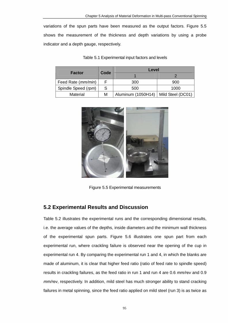
Chapter 5 Analysis of Material Deformation in Multi-pass Conventional Spinning
95
variations of the spun parts have been measured as the output factors. Figure 5.5
shows the measurement of the thickness and depth variations by using a probe
indicator and a depth gauge, respectively.
Table 5.1 Experimental input factors and levels
Level
Factor Code1 2
Feed Rate (mm/min) F 300 900 Spindle Speed (rpm) S 500 1000
Material M Aluminum (1050H14) Mild Steel (DC01)
Figure 5.5 Experimental measurements
5.2 Experimental Results and Discussion
Table 5.2 illustrates the experimental runs and the corresponding dimensional results,
i.e. the average values of the depths, inside diameters and the minimum wall thickness
of the experimental spun parts. Figure 5.6 illustrates one spun part from each
experimental run, where crackling failure is observed near the opening of the cup in
experimental run 4. By comparing the experimental run 1 and 4, in which the blanks are
made of aluminum, it is clear that higher feed ratio (ratio of feed rate to spindle speed)
results in crackling failures, as the feed ratio in run 1 and run 4 are 0.6 mm/rev and 0.9
mm/rev, respectively. In addition, mild steel has much stronger ability to stand cracking
failures in metal spinning, since the feed ratio applied on mild steel (run 3) is as twice as
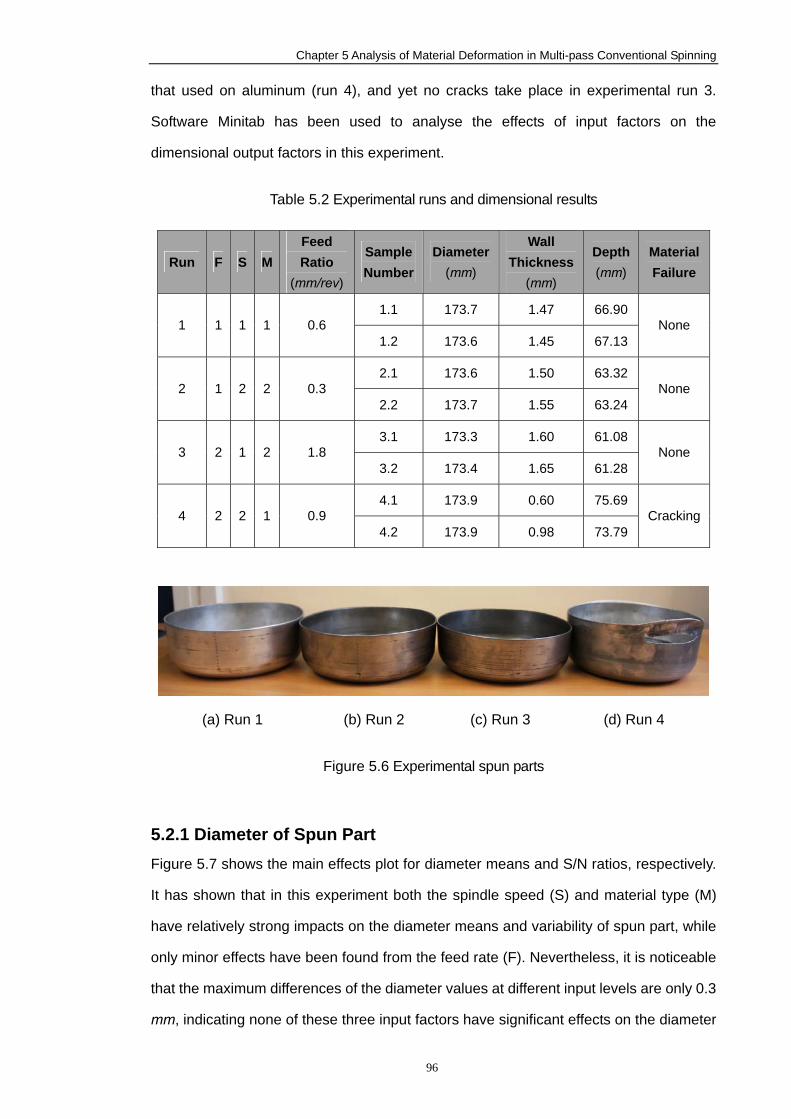
Chapter 5 Analysis of Material Deformation in Multi-pass Conventional Spinning
96
that used on aluminum (run 4), and yet no cracks take place in experimental run 3.
Software Minitab has been used to analyse the effects of input factors on the
dimensional output factors in this experiment.
Table 5.2 Experimental runs and dimensional results
Run F S M Feed Ratio
(mm/rev)
Sample Number
Diameter (mm)
Wall Thickness
(mm)
Depth (mm)
MaterialFailure
1.1 173.7 1.47 66.90 1 1 1 1 0.6
1.2 173.6 1.45 67.13 None
2.1 173.6 1.50 63.32 2 1 2 2 0.3
2.2 173.7 1.55 63.24 None
3.1 173.3 1.60 61.08 3 2 1 2 1.8
3.2 173.4 1.65 61.28 None
4.1 173.9 0.60 75.69 4 2 2 1 0.9
4.2 173.9 0.98 73.79 Cracking
(a) Run 1 (b) Run 2 (c) Run 3 (d) Run 4
Figure 5.6 Experimental spun parts
5.2.1 Diameter of Spun Part Figure 5.7 shows the main effects plot for diameter means and S/N ratios, respectively.
It has shown that in this experiment both the spindle speed (S) and material type (M)
have relatively strong impacts on the diameter means and variability of spun part, while
only minor effects have been found from the feed rate (F). Nevertheless, it is noticeable
that the maximum differences of the diameter values at different input levels are only 0.3
mm, indicating none of these three input factors have significant effects on the diameter
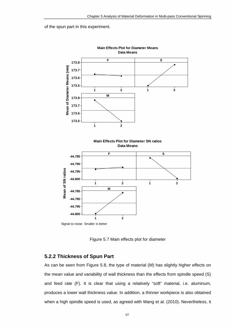
Chapter 5 Analysis of Material Deformation in Multi-pass Conventional Spinning
97
of the spun part in this experiment.
21
173.8
173.7
173.6
173.521
21
173.8
173.7
173.6
173.5
F
Mea
n of
Dia
met
er M
eans
(mm
)
S
M
Main Effects Plot for Diameter MeansData Means
21
-44.785
-44.790
-44.795
-44.80021
21
-44.785
-44.790
-44.795
-44.800
F
Mea
n of
SN
ratio
s
S
M
Main Effects Plot for Diameter SN ratiosData Means
Signal-to-noise: Smaller is better
Figure 5.7 Main effects plot for diameter
5.2.2 Thickness of Spun Part As can be seen from Figure 5.8, the type of material (M) has slightly higher effects on
the mean value and variability of wall thickness than the effects from spindle speed (S)
and feed rate (F). It is clear that using a relatively “soft” material, i.e. aluminum,
produces a lower wall thickness value. In addition, a thinner workpiece is also obtained
when a high spindle speed is used, as agreed with Wang et al. (2010). Nevertheless, it
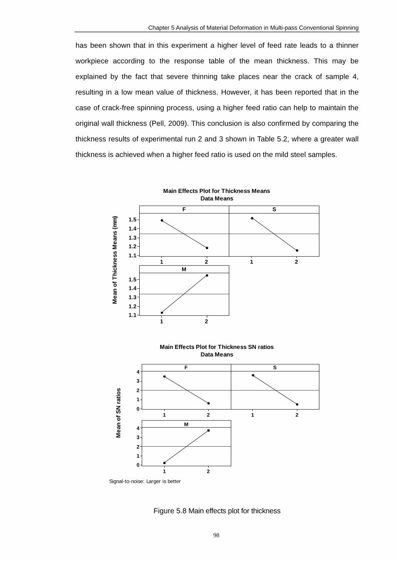
Chapter 5 Analysis of Material Deformation in Multi-pass Conventional Spinning
98
has been shown that in this experiment a higher level of feed rate leads to a thinner
workpiece according to the response table of the mean thickness. This may be
explained by the fact that severe thinning take places near the crack of sample 4,
resulting in a low mean value of thickness. However, it has been reported that in the
case of crack-free spinning process, using a higher feed ratio can help to maintain the
original wall thickness (Pell, 2009). This conclusion is also confirmed by comparing the
thickness results of experimental run 2 and 3 shown in Table 5.2, where a greater wall
thickness is achieved when a higher feed ratio is used on the mild steel samples.
21
1.51.41.31.21.1
21
21
1.51.41.31.21.1
F
Mea
n of
Thi
ckne
ss M
eans
(mm
)
S
M
Main Effects Plot for Thickness MeansData Means
21
4
3
2
1
021
21
4
3
2
1
0
F
Mea
n of
SN
ratio
s
S
M
Main Effects Plot for Thickness SN ratiosData Means
Signal-to-noise: Larger is better
Figure 5.8 Main effects plot for thickness
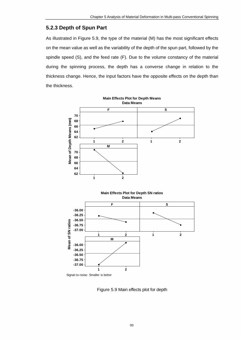
Chapter 5 Analysis of Material Deformation in Multi-pass Conventional Spinning
99
5.2.3 Depth of Spun Part
As illustrated in Figure 5.9, the type of the material (M) has the most significant effects
on the mean value as well as the variability of the depth of the spun part, followed by the
spindle speed (S), and the feed rate (F). Due to the volume constancy of the material
during the spinning process, the depth has a converse change in relation to the
thickness change. Hence, the input factors have the opposite effects on the depth than
the thickness.
21
7068666462
21
21
7068666462
F
Mea
n of
Dep
th M
eans
(mm
)
S
M
Main Effects Plot for Depth MeansData Means
21
-36.00-36.25-36.50-36.75-37.00
21
21
-36.00-36.25-36.50-36.75-37.00
F
Mea
n of
SN
ratio
s
S
M
Main Effects Plot for Depth SN ratiosData Means
Signal-to-noise: Smaller is better
Figure 5.9 Main effects plot for depth
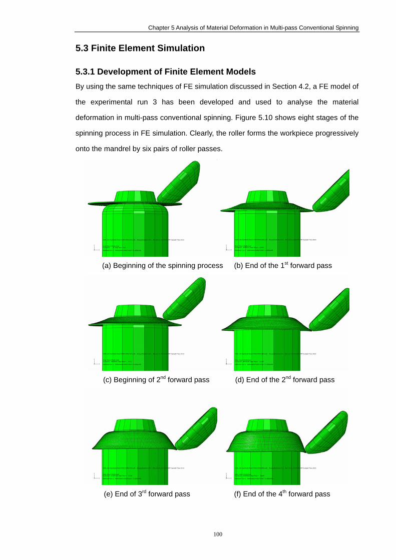
Chapter 5 Analysis of Material Deformation in Multi-pass Conventional Spinning
100
5.3 Finite Element Simulation
5.3.1 Development of Finite Element Models By using the same techniques of FE simulation discussed in Section 4.2, a FE model of
the experimental run 3 has been developed and used to analyse the material
deformation in multi-pass conventional spinning. Figure 5.10 shows eight stages of the
spinning process in FE simulation. Clearly, the roller forms the workpiece progressively
onto the mandrel by six pairs of roller passes.
(a) Beginning of the spinning process (b) End of the 1st forward pass
(c) Beginning of 2nd forward pass (d) End of the 2nd forward pass
(e) End of 3rd forward pass (f) End of the 4th forward pass
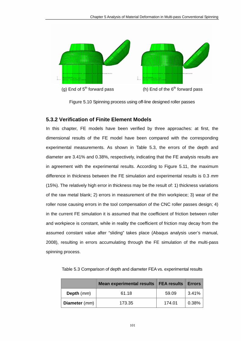
Chapter 5 Analysis of Material Deformation in Multi-pass Conventional Spinning
101
(g) End of 5th forward pass (h) End of the 6th forward pass
Figure 5.10 Spinning process using off-line designed roller passes
5.3.2 Verification of Finite Element Models In this chapter, FE models have been verified by three approaches: at first, the
dimensional results of the FE model have been compared with the corresponding
experimental measurements. As shown in Table 5.3, the errors of the depth and
diameter are 3.41% and 0.38%, respectively, indicating that the FE analysis results are
in agreement with the experimental results. According to Figure 5.11, the maximum
difference in thickness between the FE simulation and experimental results is 0.3 mm
(15%). The relatively high error in thickness may be the result of: 1) thickness variations
of the raw metal blank; 2) errors in measurement of the thin workpiece; 3) wear of the
roller nose causing errors in the tool compensation of the CNC roller passes design; 4)
in the current FE simulation it is assumed that the coefficient of friction between roller
and workpiece is constant, while in reality the coefficient of friction may decay from the
assumed constant value after “sliding” takes place (Abaqus analysis user’s manual,
2008), resulting in errors accumulating through the FE simulation of the multi-pass
spinning process.
Table 5.3 Comparison of depth and diameter FEA vs. experimental results
Mean experimental results FEA results Errors
Depth (mm) 61.18 59.09 3.41%
Diameter (mm) 173.35 174.01 0.38%
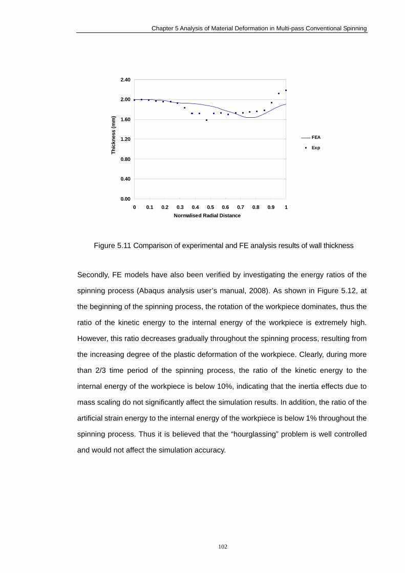
Chapter 5 Analysis of Material Deformation in Multi-pass Conventional Spinning
102
0.00
0.40
0.80
1.20
1.60
2.00
2.40
0 0.1 0.2 0.3 0.4 0.5 0.6 0.7 0.8 0.9 1Normalised Radial Distance
Thic
knes
s (m
m)
FEA
Exp
Figure 5.11 Comparison of experimental and FE analysis results of wall thickness
Secondly, FE models have also been verified by investigating the energy ratios of the
spinning process (Abaqus analysis user’s manual, 2008). As shown in Figure 5.12, at
the beginning of the spinning process, the rotation of the workpiece dominates, thus the
ratio of the kinetic energy to the internal energy of the workpiece is extremely high.
However, this ratio decreases gradually throughout the spinning process, resulting from
the increasing degree of the plastic deformation of the workpiece. Clearly, during more
than 2/3 time period of the spinning process, the ratio of the kinetic energy to the
internal energy of the workpiece is below 10%, indicating that the inertia effects due to
mass scaling do not significantly affect the simulation results. In addition, the ratio of the
artificial strain energy to the internal energy of the workpiece is below 1% throughout the
spinning process. Thus it is believed that the “hourglassing” problem is well controlled
and would not affect the simulation accuracy.
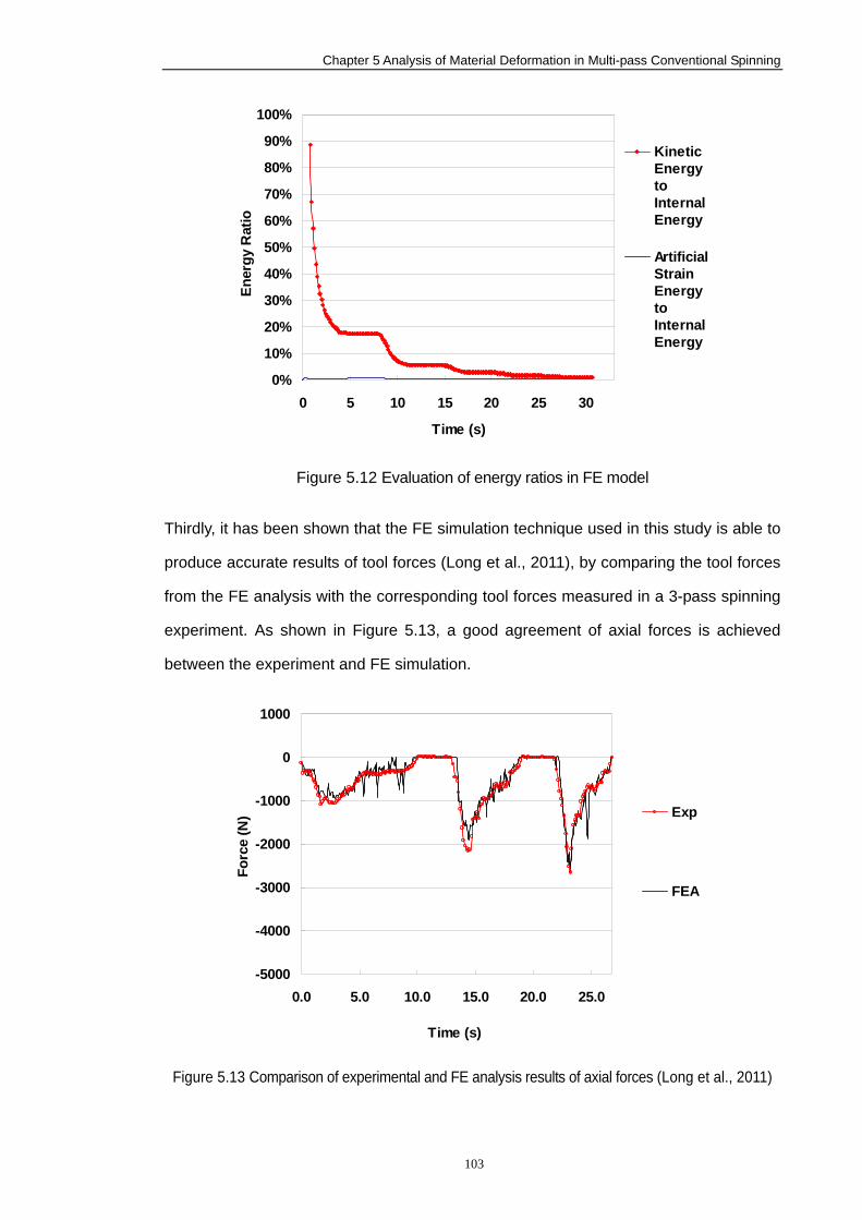
Chapter 5 Analysis of Material Deformation in Multi-pass Conventional Spinning
103
0%
10%
20%
30%
40%
50%
60%
70%
80%
90%
100%
0 5 10 15 20 25 30
Time (s)
Ener
gy R
atio
KineticEnergytoInternalEnergy
ArtificialStrainEnergytoInternalEnergy
Figure 5.12 Evaluation of energy ratios in FE model
Thirdly, it has been shown that the FE simulation technique used in this study is able to
produce accurate results of tool forces (Long et al., 2011), by comparing the tool forces
from the FE analysis with the corresponding tool forces measured in a 3-pass spinning
experiment. As shown in Figure 5.13, a good agreement of axial forces is achieved
between the experiment and FE simulation.
-5000
-4000
-3000
-2000
-1000
0
1000
0.0 5.0 10.0 15.0 20.0 25.0
Time (s)
Forc
e (N
) Exp
FEA
Figure 5.13 Comparison of experimental and FE analysis results of axial forces (Long et al., 2011)
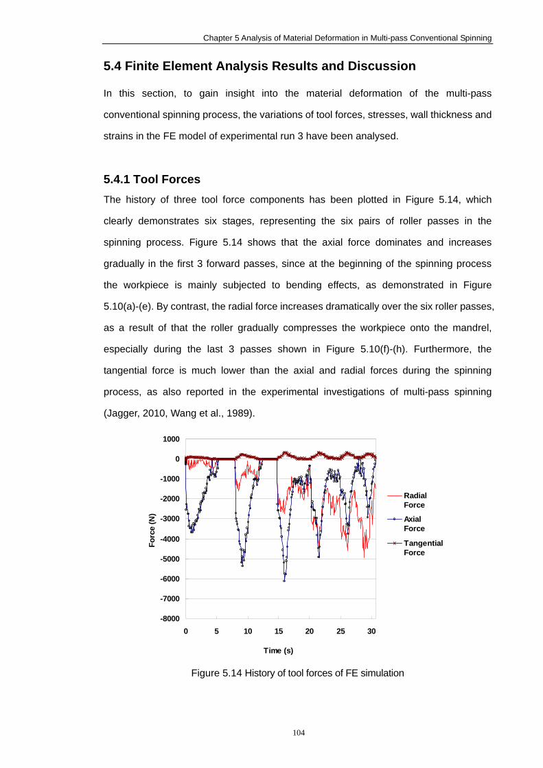
Chapter 5 Analysis of Material Deformation in Multi-pass Conventional Spinning
104
5.4 Finite Element Analysis Results and Discussion
In this section, to gain insight into the material deformation of the multi-pass
conventional spinning process, the variations of tool forces, stresses, wall thickness and
strains in the FE model of experimental run 3 have been analysed.
5.4.1 Tool Forces The history of three tool force components has been plotted in Figure 5.14, which
clearly demonstrates six stages, representing the six pairs of roller passes in the
spinning process. Figure 5.14 shows that the axial force dominates and increases
gradually in the first 3 forward passes, since at the beginning of the spinning process
the workpiece is mainly subjected to bending effects, as demonstrated in Figure
5.10(a)-(e). By contrast, the radial force increases dramatically over the six roller passes,
as a result of that the roller gradually compresses the workpiece onto the mandrel,
especially during the last 3 passes shown in Figure 5.10(f)-(h). Furthermore, the
tangential force is much lower than the axial and radial forces during the spinning
process, as also reported in the experimental investigations of multi-pass spinning
(Jagger, 2010, Wang et al., 1989).
-8000
-7000
-6000
-5000
-4000
-3000
-2000
-1000
0
1000
0 5 10 15 20 25 30
Time (s)
Forc
e (N
)
RadialForce
AxialForce
TangentialForce
Figure 5.14 History of tool forces of FE simulation
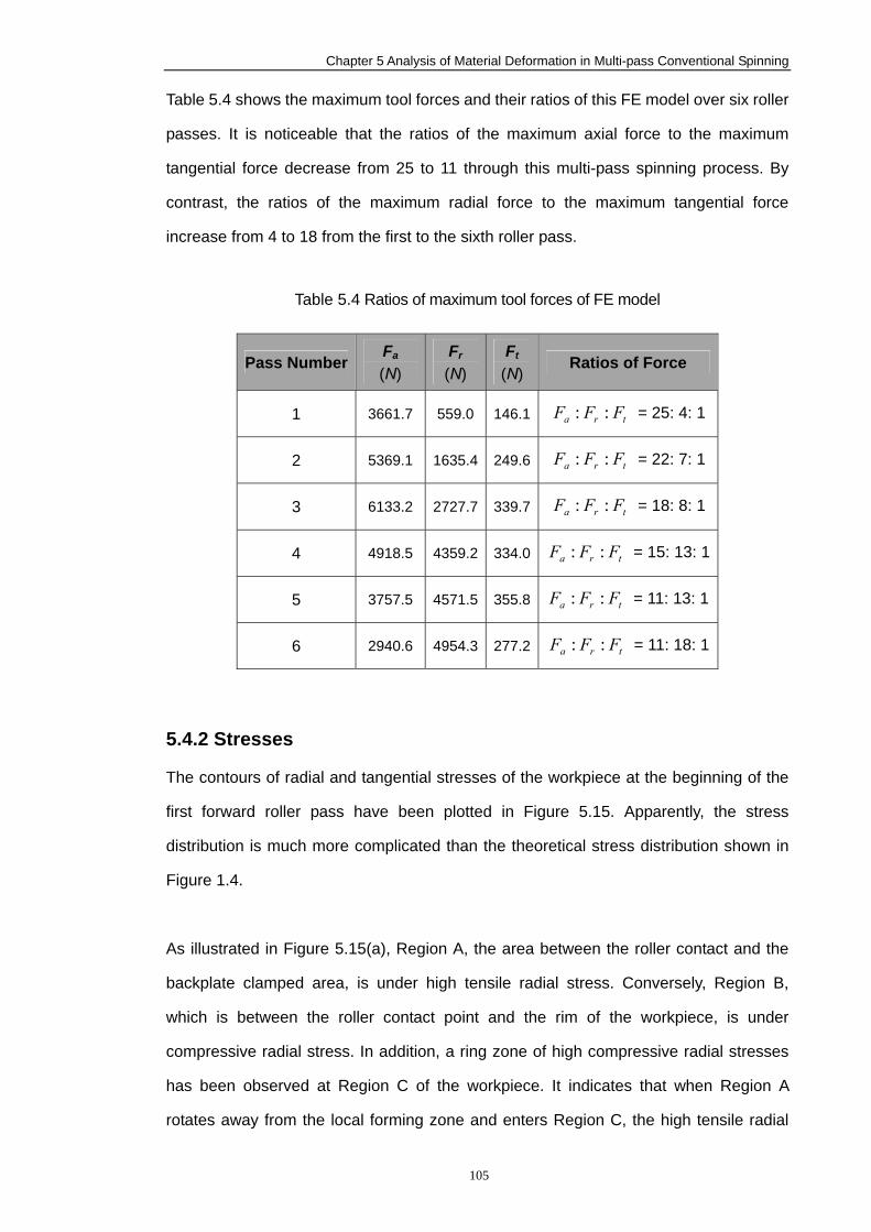
Chapter 5 Analysis of Material Deformation in Multi-pass Conventional Spinning
105
Table 5.4 shows the maximum tool forces and their ratios of this FE model over six roller
passes. It is noticeable that the ratios of the maximum axial force to the maximum
tangential force decrease from 25 to 11 through this multi-pass spinning process. By
contrast, the ratios of the maximum radial force to the maximum tangential force
increase from 4 to 18 from the first to the sixth roller pass.
Table 5.4 Ratios of maximum tool forces of FE model
Pass Number Fa
(N) Fr (N)
Ft (N)
Ratios of Force
1 3661.7 559.0 146.1 tra FFF :: = 25: 4: 1
2 5369.1 1635.4 249.6 tra FFF :: = 22: 7: 1
3 6133.2 2727.7 339.7 tra FFF :: = 18: 8: 1
4 4918.5 4359.2 334.0 tra FFF :: = 15: 13: 1
5 3757.5 4571.5 355.8 tra FFF :: = 11: 13: 1
6 2940.6 4954.3 277.2 tra FFF :: = 11: 18: 1
5.4.2 Stresses
The contours of radial and tangential stresses of the workpiece at the beginning of the
first forward roller pass have been plotted in Figure 5.15. Apparently, the stress
distribution is much more complicated than the theoretical stress distribution shown in
Figure 1.4.
As illustrated in Figure 5.15(a), Region A, the area between the roller contact and the
backplate clamped area, is under high tensile radial stress. Conversely, Region B,
which is between the roller contact point and the rim of the workpiece, is under
compressive radial stress. In addition, a ring zone of high compressive radial stresses
has been observed at Region C of the workpiece. It indicates that when Region A
rotates away from the local forming zone and enters Region C, the high tensile radial
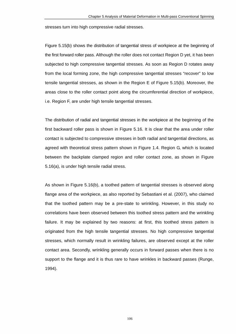
Chapter 5 Analysis of Material Deformation in Multi-pass Conventional Spinning
106
stresses turn into high compressive radial stresses.
Figure 5.15(b) shows the distribution of tangential stress of workpiece at the beginning of
the first forward roller pass. Although the roller does not contact Region D yet, it has been
subjected to high compressive tangential stresses. As soon as Region D rotates away
from the local forming zone, the high compressive tangential stresses “recover” to low
tensile tangential stresses, as shown in the Region E of Figure 5.15(b). Moreover, the
areas close to the roller contact point along the circumferential direction of workpiece,
i.e. Region F, are under high tensile tangential stresses.
The distribution of radial and tangential stresses in the workpiece at the beginning of the
first backward roller pass is shown in Figure 5.16. It is clear that the area under roller
contact is subjected to compressive stresses in both radial and tangential directions, as
agreed with theoretical stress pattern shown in Figure 1.4. Region G, which is located
between the backplate clamped region and roller contact zone, as shown in Figure
5.16(a), is under high tensile radial stress.
As shown in Figure 5.16(b), a toothed pattern of tangential stresses is observed along
flange area of the workpiece, as also reported by Sebastiani et al. (2007), who claimed
that the toothed pattern may be a pre-state to wrinkling. However, in this study no
correlations have been observed between this toothed stress pattern and the wrinkling
failure. It may be explained by two reasons: at first, this toothed stress pattern is
originated from the high tensile tangential stresses. No high compressive tangential
stresses, which normally result in wrinkling failures, are observed except at the roller
contact area. Secondly, wrinkling generally occurs in forward passes when there is no
support to the flange and it is thus rare to have wrinkles in backward passes (Runge,
1994).
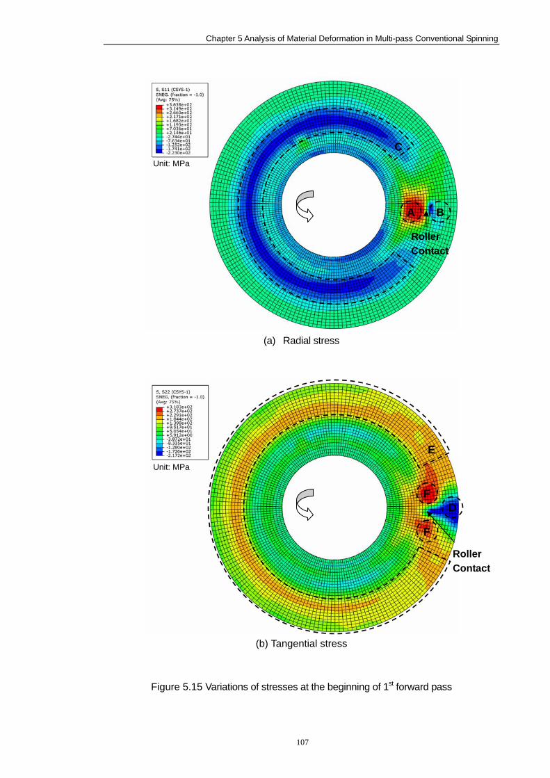
Chapter 5 Analysis of Material Deformation in Multi-pass Conventional Spinning
107
(a) Radial stress
(b) Tangential stress
Figure 5.15 Variations of stresses at the beginning of 1st forward pass
Roller Contact
C
A B
Roller Contact
F D
E
F
Unit: MPa
Unit: MPa
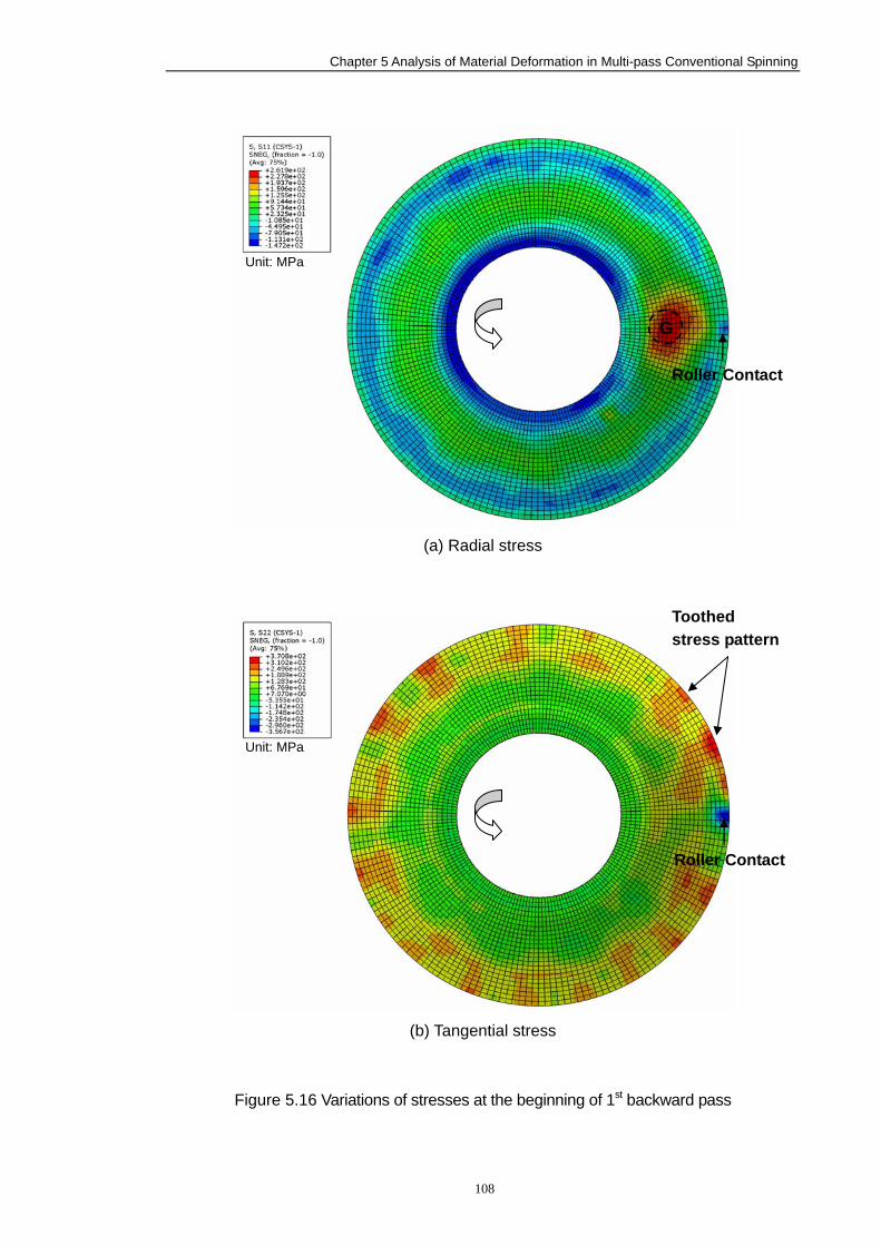
Chapter 5 Analysis of Material Deformation in Multi-pass Conventional Spinning
108
(a) Radial stress
(b) Tangential stress
Figure 5.16 Variations of stresses at the beginning of 1st backward pass
Roller Contact
Toothed stress pattern
Unit: MPa
Roller Contact
G
Unit: MPa
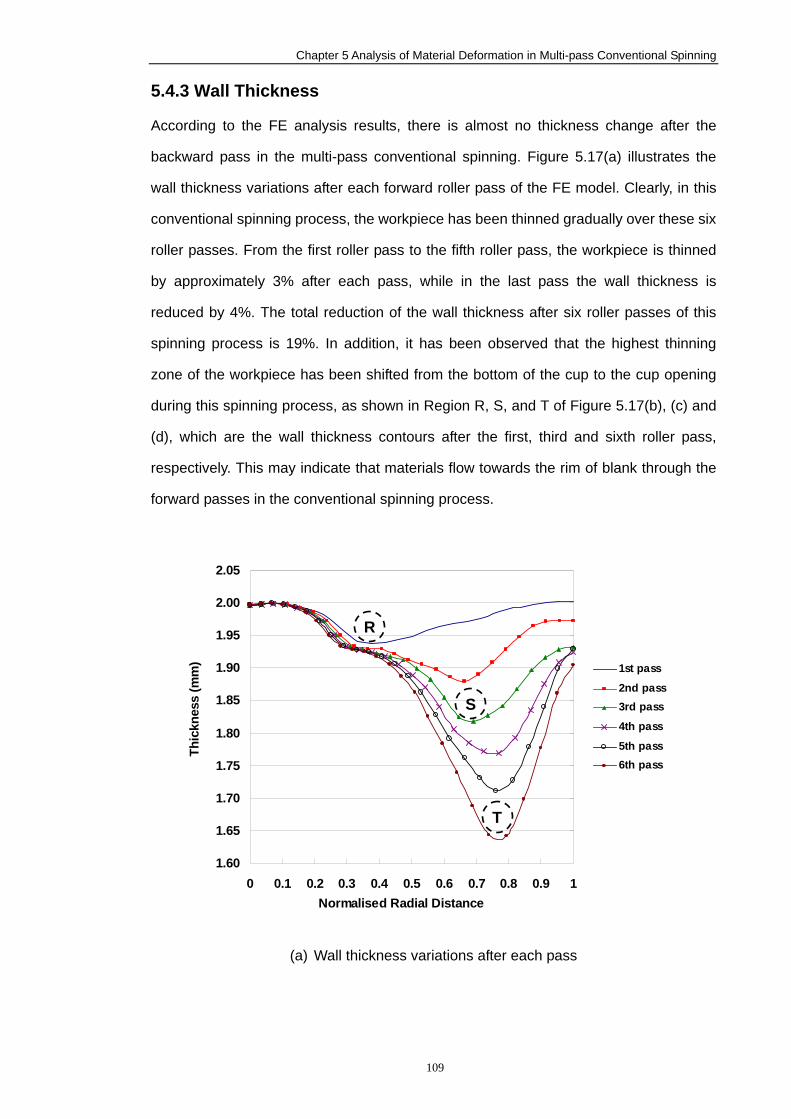
Chapter 5 Analysis of Material Deformation in Multi-pass Conventional Spinning
109
5.4.3 Wall Thickness
According to the FE analysis results, there is almost no thickness change after the
backward pass in the multi-pass conventional spinning. Figure 5.17(a) illustrates the
wall thickness variations after each forward roller pass of the FE model. Clearly, in this
conventional spinning process, the workpiece has been thinned gradually over these six
roller passes. From the first roller pass to the fifth roller pass, the workpiece is thinned
by approximately 3% after each pass, while in the last pass the wall thickness is
reduced by 4%. The total reduction of the wall thickness after six roller passes of this
spinning process is 19%. In addition, it has been observed that the highest thinning
zone of the workpiece has been shifted from the bottom of the cup to the cup opening
during this spinning process, as shown in Region R, S, and T of Figure 5.17(b), (c) and
(d), which are the wall thickness contours after the first, third and sixth roller pass,
respectively. This may indicate that materials flow towards the rim of blank through the
forward passes in the conventional spinning process.
1.60
1.65
1.70
1.75
1.80
1.85
1.90
1.95
2.00
2.05
0 0.1 0.2 0.3 0.4 0.5 0.6 0.7 0.8 0.9 1Normalised Radial Distance
Thic
knes
s (m
m) 1st pass
2nd pass3rd pass
4th pass
5th pass6th pass
(a) Wall thickness variations after each pass
T
R
S
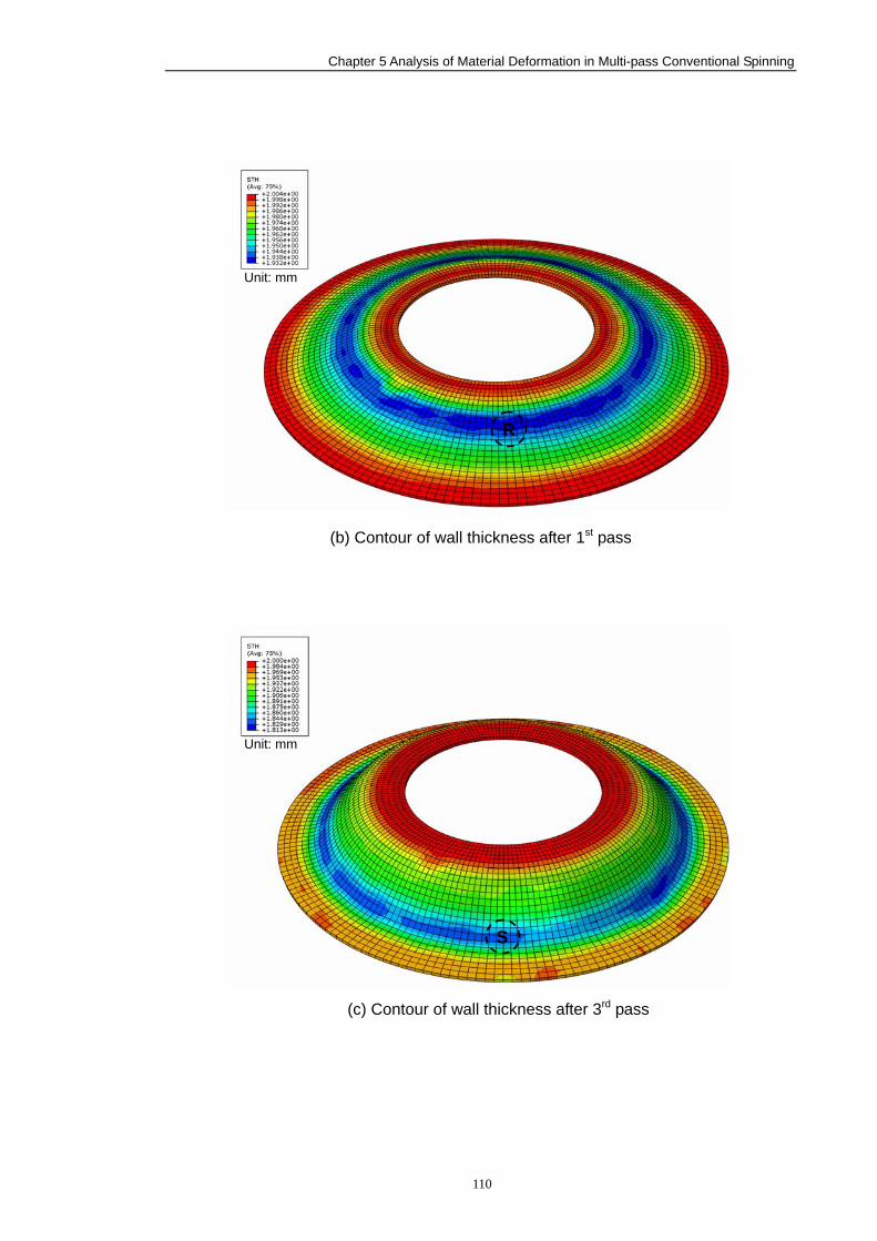
Chapter 5 Analysis of Material Deformation in Multi-pass Conventional Spinning
110
(b) Contour of wall thickness after 1st pass
(c) Contour of wall thickness after 3rd pass
R
S
Unit: mm
Unit: mm
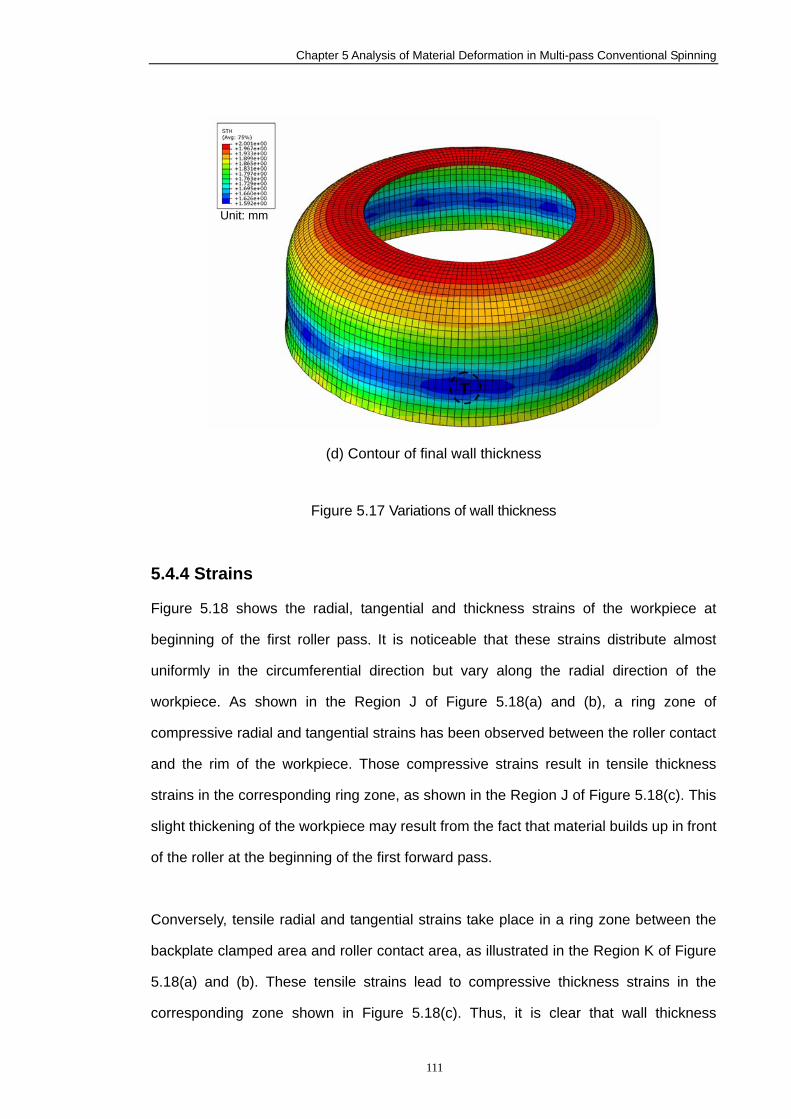
Chapter 5 Analysis of Material Deformation in Multi-pass Conventional Spinning
111
(d) Contour of final wall thickness
Figure 5.17 Variations of wall thickness
5.4.4 Strains
Figure 5.18 shows the radial, tangential and thickness strains of the workpiece at
beginning of the first roller pass. It is noticeable that these strains distribute almost
uniformly in the circumferential direction but vary along the radial direction of the
workpiece. As shown in the Region J of Figure 5.18(a) and (b), a ring zone of
compressive radial and tangential strains has been observed between the roller contact
and the rim of the workpiece. Those compressive strains result in tensile thickness
strains in the corresponding ring zone, as shown in the Region J of Figure 5.18(c). This
slight thickening of the workpiece may result from the fact that material builds up in front
of the roller at the beginning of the first forward pass.
Conversely, tensile radial and tangential strains take place in a ring zone between the
backplate clamped area and roller contact area, as illustrated in the Region K of Figure
5.18(a) and (b). These tensile strains lead to compressive thickness strains in the
corresponding zone shown in Figure 5.18(c). Thus, it is clear that wall thickness
T
Unit: mm
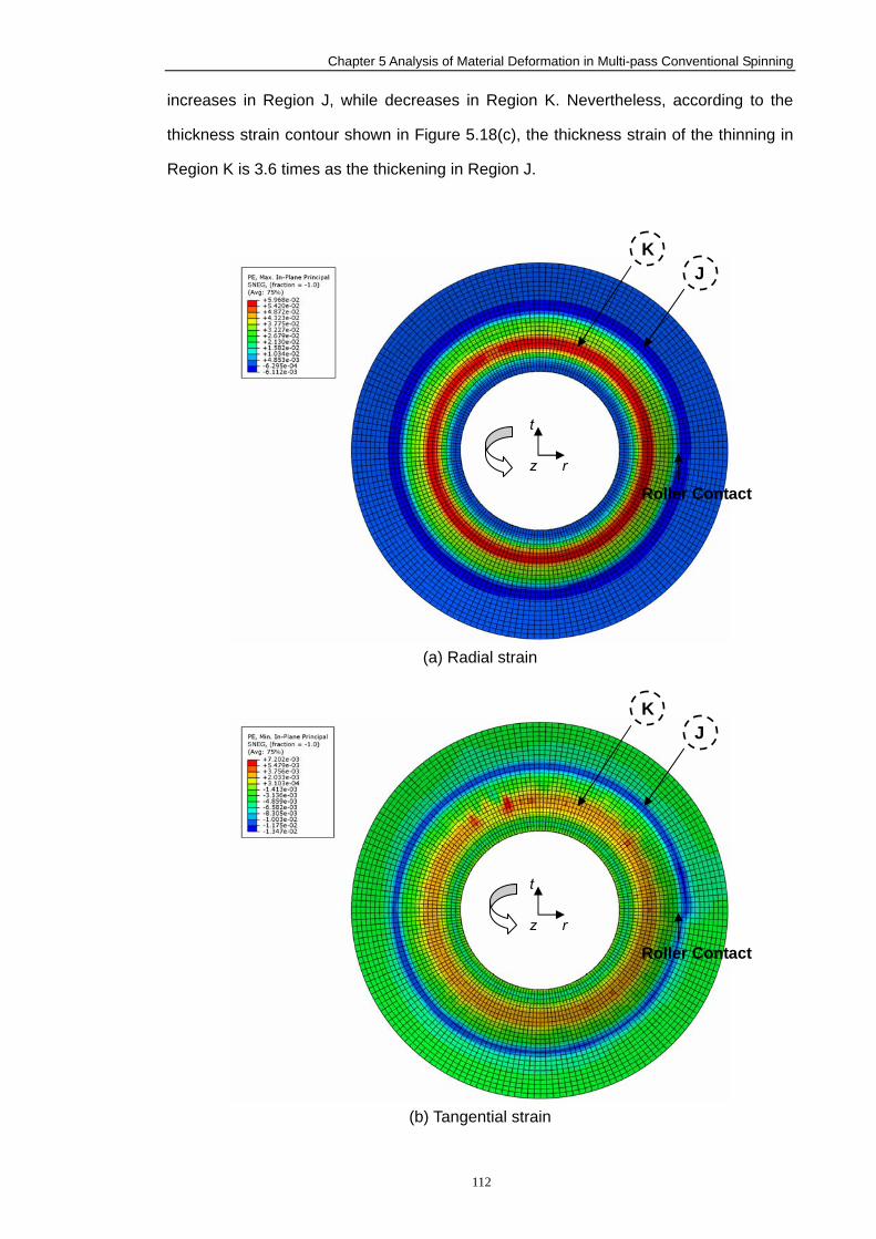
Chapter 5 Analysis of Material Deformation in Multi-pass Conventional Spinning
112
increases in Region J, while decreases in Region K. Nevertheless, according to the
thickness strain contour shown in Figure 5.18(c), the thickness strain of the thinning in
Region K is 3.6 times as the thickening in Region J.
(a) Radial strain
(b) Tangential strain
t
rz
Roller Contact
t
rz
Roller Contact
J K
J K
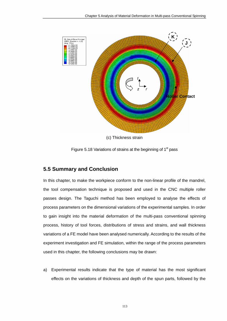
Chapter 5 Analysis of Material Deformation in Multi-pass Conventional Spinning
113
(c) Thickness strain
Figure 5.18 Variations of strains at the beginning of 1st pass
5.5 Summary and Conclusion
In this chapter, to make the workpiece conform to the non-linear profile of the mandrel,
the tool compensation technique is proposed and used in the CNC multiple roller
passes design. The Taguchi method has been employed to analyse the effects of
process parameters on the dimensional variations of the experimental samples. In order
to gain insight into the material deformation of the multi-pass conventional spinning
process, history of tool forces, distributions of stress and strains, and wall thickness
variations of a FE model have been analysed numerically. According to the results of the
experiment investigation and FE simulation, within the range of the process parameters
used in this chapter, the following conclusions may be drawn:
a) Experimental results indicate that the type of material has the most significant
effects on the variations of thickness and depth of the spun parts, followed by the
t
rz
Roller Contact
JK
Chapter 5 Analysis of Material Deformation in Multi-pass Conventional Spinning
114
spindle speed and the feed rate. However, none of these input factors show
significant effects on the diameter variations of spun parts in this experiment.
b) A high feed ratio can help to maintain the original wall thickness but cracking
failures may take place if a large feed ratio is used. Comparing with aluminum, mild
steel is much “stronger” to withstand cracking failures in the conventional spinning
process, since a feed ratio of 1.8 mm/rev is applied on mild steel blanks while a
feed ratio of 0.9 mm/rev is used on aluminum blanks, and yet no cracks take place
on the mild steel blanks.
c) According to the FE analysis results of this spinning process, the axial force is the
highest and the tangential force is the lowest. The axial force increases in the first
three passes and decreases gradually in the last three passes. Conversely, the
radial force continues to increase throughout the six roller passes.
d) Stress analysis by FE simulations shows that in the forward roller pass, high tensile
and compressive radial stresses take place behind and in front of the roller contact.
In the backward pass, a toothed tangential stress pattern has been noticed in the
flange area.
e) FE analysis results show that the wall thickness of the workpiece decreases
gradually after each forward roller pass. The thinnest zone on the workpiece has
been shifted from the bottom to the opening of the cup, while the spinning process
progresses.
f) Strains distribute almost uniformly in the circumferential direction but vary along the
radial direction of the workpiece. At the beginning of a forward pass, a ring zone of
tensile radial and tangential strains has been observed between the backplate
clamped area and the roller contact zone, resulting in compressive thickness
strains, i.e. wall thinning.
Chapter 6 Study on Wrinkling Failures
115
6. Study on Wrinkling Failures
In this chapter, wrinkling failure in conventional spinning has been studied by theoretical
analysis, experimental investigation and Finite Element simulation. The energy method
and two-directional plate buckling theory have been used to predict the critical condition
of wrinkling failure in conventional spinning. The severity of wrinkles is quantified by
calculating the standard deviation of the radial coordinates of element nodes on the
edge of the workpiece obtained from the FE models. A forming limit study for wrinkling
has been carried out and it shows there is a feed ratio limit beyond which wrinkling
failures will take place. It is believed that if the high compressive tangential stresses in
the local forming zone do not “recover” to tensile tangential stresses after roller contact,
wrinkling failure will occur. Furthermore, the computational performance of the solid and
shell elements in simulating the spinning process is examined.
6.1 Theoretical Analysis
It is believed that wrinkling in sheet metal forming is a local phenomenon, which
depends on the local curvatures and stress states (Hutchinson and Neale, 1985).
Hence, the region being investigated for flange wrinkling may be simplified as a
rectangular plate (Wang and Cao, 2000), as shown in Figure 6.1. The length of a
half-wave wrinkled flange in the tangential direction (x axis) is a; the width of the
wrinkled flange in the radial direction (y axis) is b. The following assumptions have been
made in order to simplify the theoretical analysis:
1) Shear stresses are neglected;
2) No dynamic effects are considered;
3) Wall thickness remains constant throughout the spinning process;
4) The loading of roller is simplified as a lateral concentrated load P, perpendicular
to the plate.
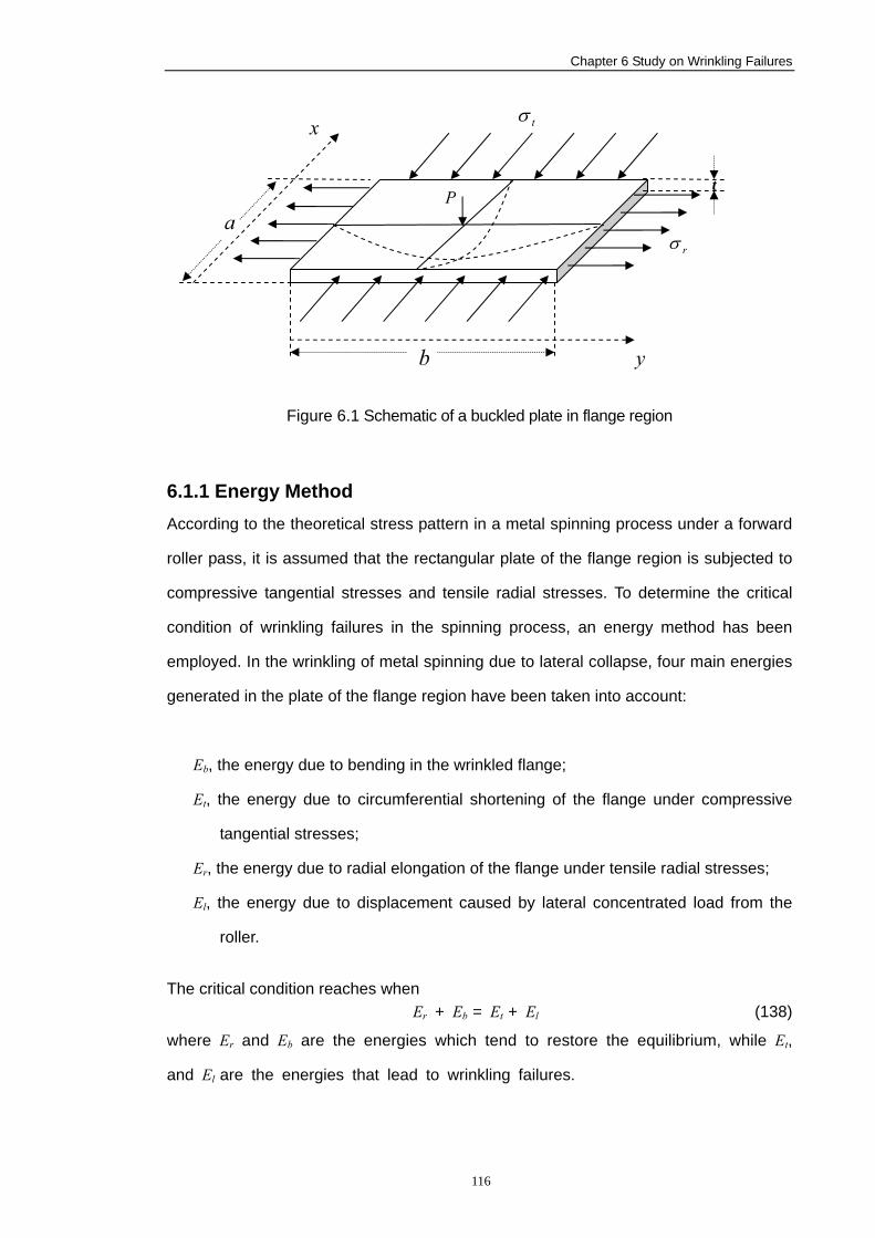
Chapter 6 Study on Wrinkling Failures
116
Figure 6.1 Schematic of a buckled plate in flange region
6.1.1 Energy Method
According to the theoretical stress pattern in a metal spinning process under a forward
roller pass, it is assumed that the rectangular plate of the flange region is subjected to
compressive tangential stresses and tensile radial stresses. To determine the critical
condition of wrinkling failures in the spinning process, an energy method has been
employed. In the wrinkling of metal spinning due to lateral collapse, four main energies
generated in the plate of the flange region have been taken into account:
Eb, the energy due to bending in the wrinkled flange;
Et, the energy due to circumferential shortening of the flange under compressive
tangential stresses;
Er, the energy due to radial elongation of the flange under tensile radial stresses;
El, the energy due to displacement caused by lateral concentrated load from the
roller.
The critical condition reaches when
Er + Eb = Et + El (138)
where Er and Eb are the energies which tend to restore the equilibrium, while Et,
and El are the energies that lead to wrinkling failures.
rσ
b y
a
x
t P
tσ
Chapter 6 Study on Wrinkling Failures
117
6.1.2 Theoretical Model Assuming that the buckled deflection surface, as illustrated by the dotted curves in
Figure 6.1, is given by the equation (Timoshenko, 1936):
by
axw ππγ sinsin= (139)
where γ is the maximum deflection of the buckling surface.
The energy due to bending can be calculated by (Timoshenko, 1936):
( )∫ ∫⎪⎭
⎪⎬⎫
⎪⎩
⎪⎨⎧
⎥⎥⎦
⎤
⎢⎢⎣
⎡⎟⎟⎠
⎞⎜⎜⎝
⎛∂∂
∂−
∂∂
∂∂
−−⎟⎟⎠
⎞⎜⎜⎝
⎛∂∂
+∂∂
=b a
b dxdyyx
wyw
xw
yw
xwDE
0 0
22
2
2
2
22
2
2
2
2
1221 ν (140)
Substituting (139) into (140),
2
2
2
2
22
8 ⎟⎟⎠
⎞⎜⎜⎝
⎛+=
baDabEb
ππγ (141)
where D is the flexural rigidity of plate
( )2
3
112 ν−=
EtD (142)
where E is the Young’s Modulus, t is the wall thickness, v is the Poisson’s ratio. It has
been shown that the elastic bending theory can be extended to cover plastic bending by
replacing E with the reduced modulus E0 (Gere, 2001):
( )20
4
p
p
EE
EEE
+= (143)
where Ep is the slope of the stress-strain curve at a particular value of strain in the
plastic region.
The energy due to tangential stress tσ can be calculated by
∫ ∫ ⎟⎠⎞
⎜⎝⎛∂∂
=a b
tt dxdyxwtE
0 0
2
21 σ (144)
Substituting (139) into (144), we obtain
atb
E tt 8
22 σπγ= (145)
Chapter 6 Study on Wrinkling Failures
118
The energy due to radial stress rσ can be calculated by
∫ ∫ ⎟⎟⎠
⎞⎜⎜⎝
⎛∂∂
=b a
rr dydxywtE
0 0
2
21 σ (146)
Substituting (139) into (146), we obtain
btaE r
r 8
22 σπγ= (147)
According to Timoshenko and Woinowsky-Krieger (1959), the deflection resulting from a
concentrated load P can be expressed as
DPbw
2
α= (148)
whereα is a numerical factor, the value of which depends on the ratio of a/b and is given
in Table 6.1.
Table 6.1 Factorα for deflection equation (Timoshenko and Woinowsky-Krieger, 1959)
a/b 1.0 1.1 1.2 1.4 1.6 1.8 2.0 3 ∞
α 0.01160 0.01265 0.01353 0.01484 0.01570 0.01620 0.01651 0.01690 0.01695
The lateral energy El due to the concentrated loading P can be calculated as:
∫ ==γ
αγ
02
2
2 bDPdwEl (149)
Substituting (141), (145), (147) and (149) into (138), we have
32
2
2
22
2
2
2
2 4abD
at
bt
baD tr α
σπσπππ+=+⎟⎟
⎠
⎞⎜⎜⎝
⎛+ (150)
Dividing Equation (150) by 2
2
atπ
and introducing notations eσ andλ , where
taD
e 2
2πσ = (151)
ba
=λ (152)
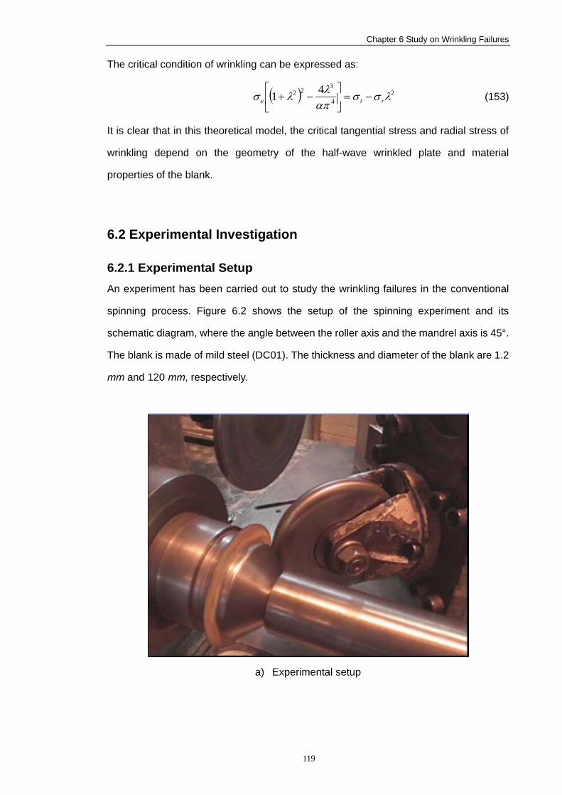
Chapter 6 Study on Wrinkling Failures
119
The critical condition of wrinkling can be expressed as:
( ) 24
322 41 λσσ
απλλσ rte −=⎥
⎦
⎤⎢⎣
⎡−+ (153)
It is clear that in this theoretical model, the critical tangential stress and radial stress of
wrinkling depend on the geometry of the half-wave wrinkled plate and material
properties of the blank.
6.2 Experimental Investigation
6.2.1 Experimental Setup An experiment has been carried out to study the wrinkling failures in the conventional
spinning process. Figure 6.2 shows the setup of the spinning experiment and its
schematic diagram, where the angle between the roller axis and the mandrel axis is 45°.
The blank is made of mild steel (DC01). The thickness and diameter of the blank are 1.2
mm and 120 mm, respectively.
a) Experimental setup
Chapter 6 Study on Wrinkling Failures
120
b) Schematic diagram
Figure 6.2 Spinning experiment of wrinkling investigation
6.2.2 Process Parameters Figure 6.3 illustrates the roller passes used in the experiment, clearly only the two
forward passes are effective as the backward pass does not deform the blank. Table 6.2
shows the process parameters used in four experimental runs. In an experimental run,
the feed rate in the axial direction of the roller (z-axis in Figure 6.2b) is almost constant,
while the feed rate in the radial direction of the roller (x-axis in Figure 6.2b) changes with
time. 300% and 600% of the initial feed rate used in experimental run E1 are applied to
experimental run E2 and E3, respectively. Only the first pass of experimental run E3 is
used in experimental run E4.
Chapter 6 Study on Wrinkling Failures
121
-5
-4
-3
-2
-1
0
1
2
3
4
5
-30 -25 -20 -15 -10 -5 0
Y (mm)
X (m
m)
1st forwardpassBackwardpass2nd forwardpass
Figure 6.3 Roller passes used in the experiment
Table 6.2 Process parameters of experimental runs
Sample Number Spindle Speed
(rpm) Longitudinal Feed Rate (z-axis)
(mm/min)
E1 400 212 (Initial feed rate)
E2 400 300% of Initial feed rate
E3 400 600% of Initial feed rate
E4 400 600% of Initial feed rate
(only the first roller pass is applied)
As shown in Figure 6.4(a), sample E1 has no wrinkles with relatively smooth surface.
Increasing the initial feed rate by 300% and 600%, the surface of the sample E2 and E3
become rough accordingly, as shown in Figure 6.4(b) and 6.4(c). In addition, by
comparing the experimental spun part E3 and E4 of Figure 6.4(c) and 6.4(d), it is clear
that wrinkling occurs in the first pass, and then smoothed out during the second pass.
However, the high feed rate of the roller pass leads to extremely rough surface finish,
which also reported by Chen et al. (2001).
X
Y
Chapter 6 Study on Wrinkling Failures
122
Figure 6.4 Experimental samples
6.3 Finite Element Simulation
Since the wrinkling failures only take place in the first forward roller pass of this
experiment, the backward pass and the second forward pass are neglected in the FE
simulation. The information of the roller pass has been given in the Appendix 2. Table
6.3 presents the process parameters of some of the FE models and the corresponding
flange states. The mass scaling technique is used in these FE models to speed up the
computation. A mass scaling factor of 25 has been used in Model 1 - 6, in which the
spindle speed varies between 400 rpm to 800 rpm. Conversely, no mass scaling is used
in Model 7, which applies a significantly high spindle speed – 1800 rpm, in order to
prevent the inertial effects due to mass scaling. The first three models (Model 1 - Model
3) use the same setting as experimental sample E1, E2 and E4.
(a) E1 (b) E2
(c) E3 (d) E4
Chapter 6 Study on Wrinkling Failures
123
Table 6.3 FE analysis process parameters and flange state of spun part
Model Replay
feed rate
Feed rate
(mm/min)
Spindle speed (rpm)
Mass scaling factor
Feed ratio
(mm/r)
Process duration
(s)
Flange state
Model 1 100% 212 400 25 0.53 5.44 No wrinklesModel 2 300% 636 400 25 1.59 1.81 Wrinkling Model 3 600% 1272 400 25 3.18 0.91 Wrinkling Model 4 800% 1696 800 25 2.12 0.68 Wrinkling Model 5 200% 424 600 25 0.71 2.72 No wrinklesModel 6 600% 1272 800 25 1.59 0.91 Wrinkling Model 7 600% 1272 1800 1 0.71 0.91 No wrinkles
6.3.1 Element Selection To evaluate the performance of the 8 noded reduced integration linear solid element
(C3D8R) and the 8 noded reduced integration linear continuum shell element (SC8R)
for the wrinkling simulation of the spinning process, three FE models have been
compared using the experimental setting of sample E4. Detailed meshing information is
shown in Table 6.4, where Model 3a and 3b applied the same process parameters as
Model 3 defined in Table 6.3, but with different element types and number of elements
through thickness direction of the blank.
Table 6.4 FE models using different types and numbers of elements
Model Type of element
Elements through
thickness
Number of
element
Stable increment
(s)
CPU time
(h:m:s)
Flange state
Model 3a
C3D8R 1 5200 4.71e-7 08:51:12 No
wrinklesModel
3b C3D8R 4 20800 1.37e-7 48:09:38
Minor wrinkles
Wrinkling Model
Model 3
SC8R 1 5200 5.66e-7 14:18:07 Severe wrinkles
Model 5a
C3D8R 1 5200 5.12e-7 13:14:48 No
wrinklesModel
5b C3D8R 4 20800 2.12e-7 62:55:34
No wrinkles
Wrinkle -free
Model Model
5 SC8R 1 5200 5.66e-7 21:44:38
No wrinkles
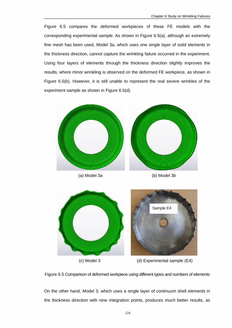
Chapter 6 Study on Wrinkling Failures
124
Figure 6.5 compares the deformed workpieces of these FE models with the
corresponding experimental sample. As shown in Figure 6.5(a), although an extremely
fine mesh has been used, Model 3a, which uses one single layer of solid elements in
the thickness direction, cannot capture the wrinkling failure occurred in the experiment.
Using four layers of elements through the thickness direction slightly improves the
results, where minor wrinkling is observed on the deformed FE workpiece, as shown in
Figure 6.5(b). However, it is still unable to represent the real severe wrinkles of the
experiment sample as shown in Figure 6.5(d).
(a) Model 3a (b) Model 3b
(c) Model 3 (d) Experimental sample (E4)
Figure 6.5 Comparison of deformed workpiece using different types and numbers of elements
On the other hand, Model 3, which uses a single layer of continuum shell elements in
the thickness direction with nine integration points, produces much better results, as
Sample E4
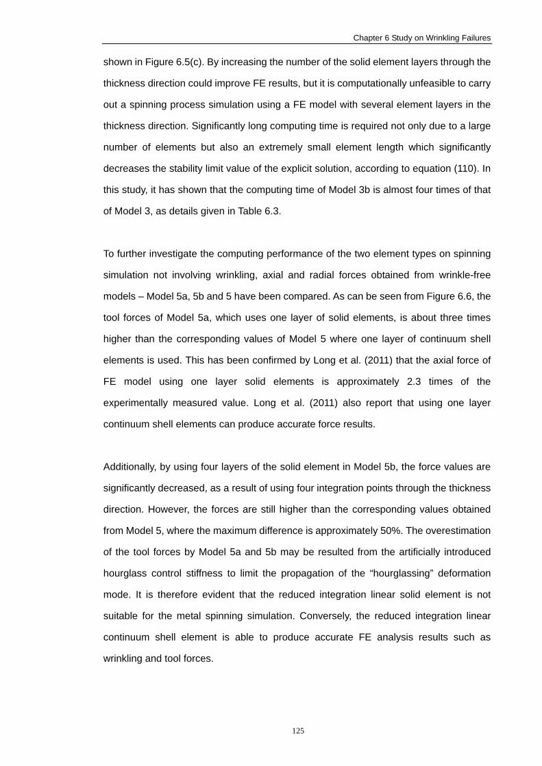
Chapter 6 Study on Wrinkling Failures
125
shown in Figure 6.5(c). By increasing the number of the solid element layers through the
thickness direction could improve FE results, but it is computationally unfeasible to carry
out a spinning process simulation using a FE model with several element layers in the
thickness direction. Significantly long computing time is required not only due to a large
number of elements but also an extremely small element length which significantly
decreases the stability limit value of the explicit solution, according to equation (110). In
this study, it has shown that the computing time of Model 3b is almost four times of that
of Model 3, as details given in Table 6.3.
To further investigate the computing performance of the two element types on spinning
simulation not involving wrinkling, axial and radial forces obtained from wrinkle-free
models – Model 5a, 5b and 5 have been compared. As can be seen from Figure 6.6, the
tool forces of Model 5a, which uses one layer of solid elements, is about three times
higher than the corresponding values of Model 5 where one layer of continuum shell
elements is used. This has been confirmed by Long et al. (2011) that the axial force of
FE model using one layer solid elements is approximately 2.3 times of the
experimentally measured value. Long et al. (2011) also report that using one layer
continuum shell elements can produce accurate force results.
Additionally, by using four layers of the solid element in Model 5b, the force values are
significantly decreased, as a result of using four integration points through the thickness
direction. However, the forces are still higher than the corresponding values obtained
from Model 5, where the maximum difference is approximately 50%. The overestimation
of the tool forces by Model 5a and 5b may be resulted from the artificially introduced
hourglass control stiffness to limit the propagation of the “hourglassing” deformation
mode. It is therefore evident that the reduced integration linear solid element is not
suitable for the metal spinning simulation. Conversely, the reduced integration linear
continuum shell element is able to produce accurate FE analysis results such as
wrinkling and tool forces.
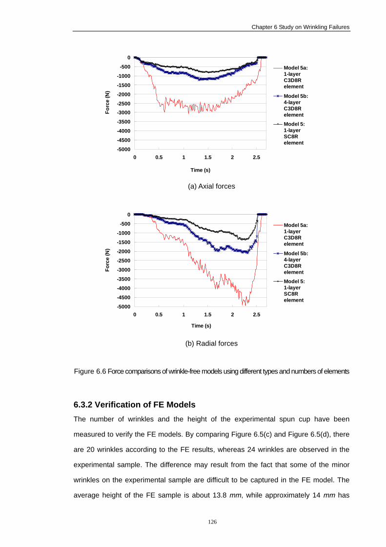
Chapter 6 Study on Wrinkling Failures
126
-5000
-4500
-4000
-3500
-3000-2500
-2000
-1500
-1000
-500
0
0 0.5 1 1.5 2 2.5
Time (s)
Forc
e (N
)
Model 5a:1-layerC3D8Relement
Model 5b:4-layerC3D8Relement
Model 5:1-layerSC8Relement
(a) Axial forces
-5000
-4500
-4000
-3500
-3000
-2500
-2000
-1500
-1000
-500
0
0 0.5 1 1.5 2 2.5
Time (s)
Forc
e (N
)
Model 5a:1-layerC3D8Relement
Model 5b:4-layerC3D8Relement
Model 5:1-layerSC8Relement
(b) Radial forces
Figure 6.6 Force comparisons of wrinkle-free models using different types and numbers of elements
6.3.2 Verification of FE Models The number of wrinkles and the height of the experimental spun cup have been
measured to verify the FE models. By comparing Figure 6.5(c) and Figure 6.5(d), there
are 20 wrinkles according to the FE results, whereas 24 wrinkles are observed in the
experimental sample. The difference may result from the fact that some of the minor
wrinkles on the experimental sample are difficult to be captured in the FE model. The
average height of the FE sample is about 13.8 mm, while approximately 14 mm has
Chapter 6 Study on Wrinkling Failures
127
been measured from the experimental sample. Therefore it is believed that the FE
analysis results are in agreement with the experimental results.
Figure 6.7 compares the ratios of the artificial strain energies to the internal energies
from the three wrinkle-free models – Model 5a, 5b and 5. It is clear that the energy ratio
is around 1% throughout the whole spinning process in Model 5 which uses one layer
continuum shell elements, demonstrating that “hourglassing” is not an issue in this
model. However, the energy ratio is extremely high in Model 5a with one layer of solid
elements. It shows that “hourglassing” is a major problem which could significantly
affect the results. By using 4 layers of solid elements in Model 5b, this energy ratio has
decreased dramatically but is still much higher than the energy ratio obtained from
Model 5.
0
0.1
0.2
0.3
0.4
0.5
0.6
0.7
0.8
0.9
0 0.5 1 1.5 2 2.5
Time (s)
Ener
gy R
atio
Model 5a:1-layerC3D8Relement
Model 5b:4-layerC3D8Relement
Model 5:1-layerSC8Relement
Figure 6.7 Ratio of artificial strain energy to internal energy of the wrinkle-free models
6.4 Results and Discussion
In this section, an approach to quantify the severity of wrinkles is proposed. A forming
limit diagram is drawn based on results of a number of FE models using various feed
rates and spindle speeds. Furthermore, the variations of tool forces, stresses and wall
thickness have been studied numerically. The theoretical analysis model of wrinkling is
verified by comparing the theoretical stress state with the FE analysis stress results.
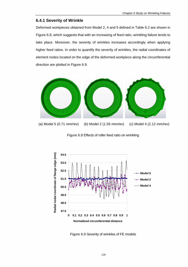
Chapter 6 Study on Wrinkling Failures
128
6.4.1 Severity of Wrinkle Deformed workpieces obtained from Model 2, 4 and 5 defined in Table 6.2 are shown in
Figure 6.8, which suggests that with an increasing of feed ratio, wrinkling failure tends to
take place. Moreover, the severity of wrinkles increases accordingly when applying
higher feed ratios. In order to quantify the severity of wrinkles, the radial coordinates of
element nodes located on the edge of the deformed workpiece along the circumferential
direction are plotted in Figure 6.9.
(a) Model 5 (0.71 mm/rev) (b) Model 2 (1.59 mm/rev) (c) Model 4 (2.12 mm/rev)
Figure 6.8 Effects of roller feed ratio on wrinkling
47.5
48.5
49.5
50.5
51.5
52.5
53.5
54.5
0 0.1 0.2 0.3 0.4 0.5 0.6 0.7 0.8 0.9 1
Normalised circumferential distance
Rad
ial n
odal
coo
rdin
ate
of fl
ange
edg
e (m
m)
Model 5
Model 2
Model 4
Figure 6.9 Severity of wrinkles of FE models
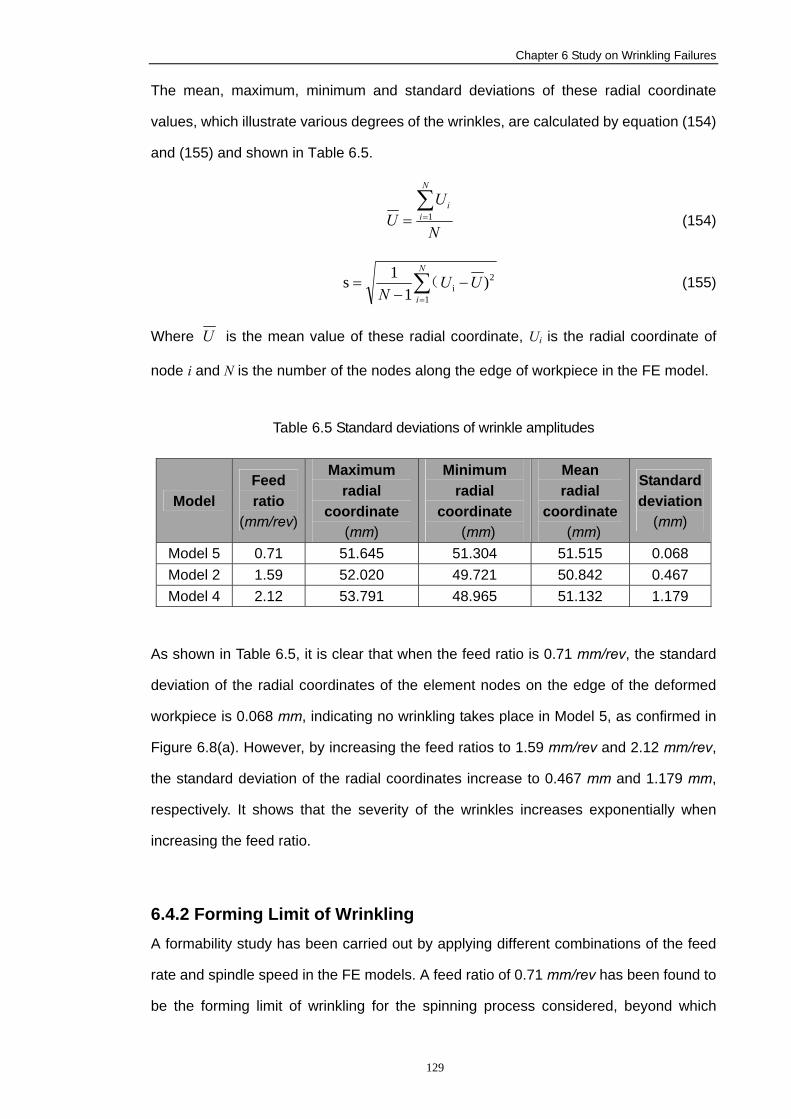
Chapter 6 Study on Wrinkling Failures
129
The mean, maximum, minimum and standard deviations of these radial coordinate
values, which illustrate various degrees of the wrinkles, are calculated by equation (154)
and (155) and shown in Table 6.5.
N
UU
N
ii∑
== 1 (154)
2
1i )
11s ∑
=
−−
=N
iUU
N( (155)
Where U is the mean value of these radial coordinate, Ui is the radial coordinate of
node i and N is the number of the nodes along the edge of workpiece in the FE model.
Table 6.5 Standard deviations of wrinkle amplitudes
Model Feed ratio
(mm/rev)
Maximum radial
coordinate (mm)
Minimum radial
coordinate (mm)
Mean radial
coordinate (mm)
Standard deviation
(mm)
Model 5 0.71 51.645 51.304 51.515 0.068 Model 2 1.59 52.020 49.721 50.842 0.467 Model 4 2.12 53.791 48.965 51.132 1.179
As shown in Table 6.5, it is clear that when the feed ratio is 0.71 mm/rev, the standard
deviation of the radial coordinates of the element nodes on the edge of the deformed
workpiece is 0.068 mm, indicating no wrinkling takes place in Model 5, as confirmed in
Figure 6.8(a). However, by increasing the feed ratios to 1.59 mm/rev and 2.12 mm/rev,
the standard deviation of the radial coordinates increase to 0.467 mm and 1.179 mm,
respectively. It shows that the severity of the wrinkles increases exponentially when
increasing the feed ratio.
6.4.2 Forming Limit of Wrinkling A formability study has been carried out by applying different combinations of the feed
rate and spindle speed in the FE models. A feed ratio of 0.71 mm/rev has been found to
be the forming limit of wrinkling for the spinning process considered, beyond which
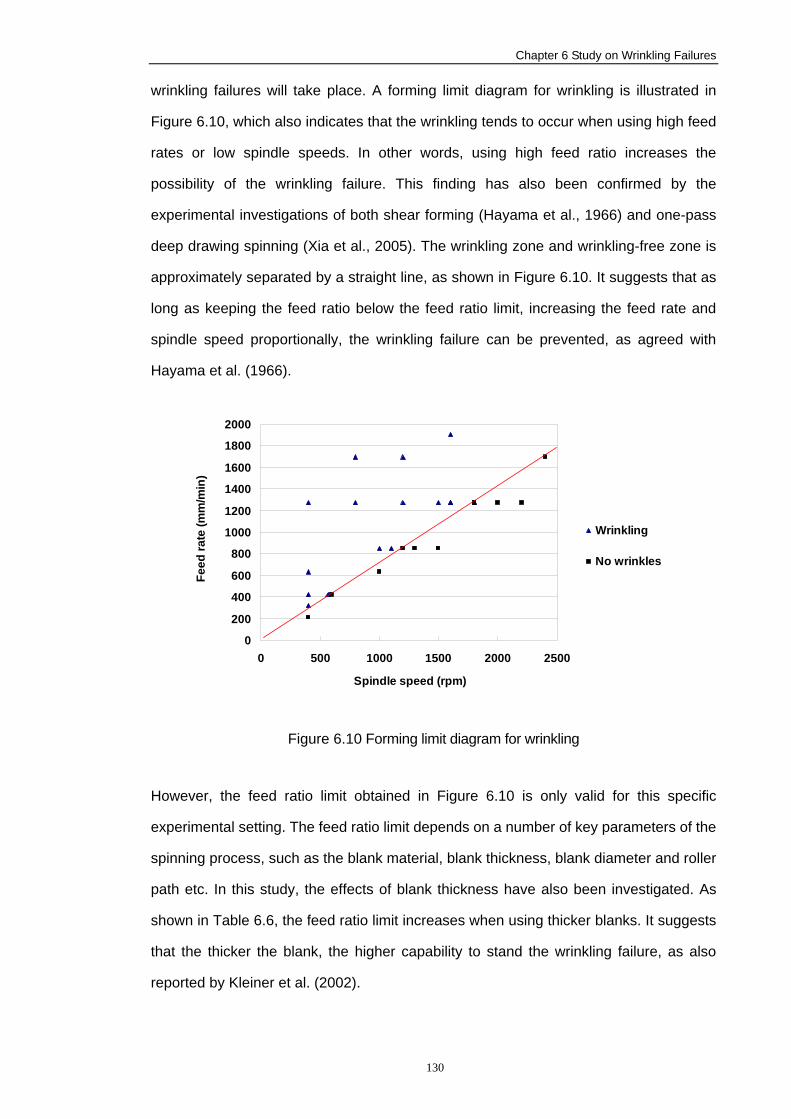
Chapter 6 Study on Wrinkling Failures
130
wrinkling failures will take place. A forming limit diagram for wrinkling is illustrated in
Figure 6.10, which also indicates that the wrinkling tends to occur when using high feed
rates or low spindle speeds. In other words, using high feed ratio increases the
possibility of the wrinkling failure. This finding has also been confirmed by the
experimental investigations of both shear forming (Hayama et al., 1966) and one-pass
deep drawing spinning (Xia et al., 2005). The wrinkling zone and wrinkling-free zone is
approximately separated by a straight line, as shown in Figure 6.10. It suggests that as
long as keeping the feed ratio below the feed ratio limit, increasing the feed rate and
spindle speed proportionally, the wrinkling failure can be prevented, as agreed with
Hayama et al. (1966).
0
200
400
600
800
1000
1200
1400
1600
1800
2000
0 500 1000 1500 2000 2500
Spindle speed (rpm)
Feed
rate
(mm
/min
)
Wrinkling
No wrinkles
Figure 6.10 Forming limit diagram for wrinkling
However, the feed ratio limit obtained in Figure 6.10 is only valid for this specific
experimental setting. The feed ratio limit depends on a number of key parameters of the
spinning process, such as the blank material, blank thickness, blank diameter and roller
path etc. In this study, the effects of blank thickness have also been investigated. As
shown in Table 6.6, the feed ratio limit increases when using thicker blanks. It suggests
that the thicker the blank, the higher capability to stand the wrinkling failure, as also
reported by Kleiner et al. (2002).
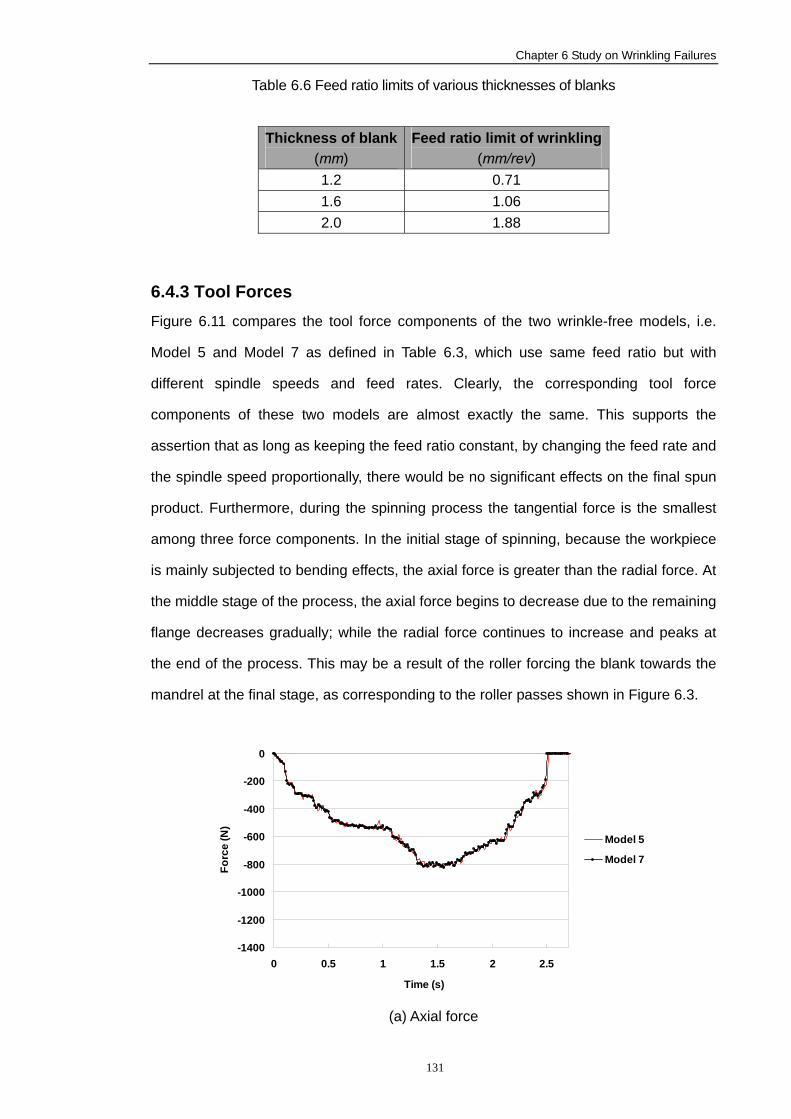
Chapter 6 Study on Wrinkling Failures
131
Table 6.6 Feed ratio limits of various thicknesses of blanks
Thickness of blank(mm)
Feed ratio limit of wrinkling (mm/rev)
1.2 0.71 1.6 1.06 2.0 1.88
6.4.3 Tool Forces Figure 6.11 compares the tool force components of the two wrinkle-free models, i.e.
Model 5 and Model 7 as defined in Table 6.3, which use same feed ratio but with
different spindle speeds and feed rates. Clearly, the corresponding tool force
components of these two models are almost exactly the same. This supports the
assertion that as long as keeping the feed ratio constant, by changing the feed rate and
the spindle speed proportionally, there would be no significant effects on the final spun
product. Furthermore, during the spinning process the tangential force is the smallest
among three force components. In the initial stage of spinning, because the workpiece
is mainly subjected to bending effects, the axial force is greater than the radial force. At
the middle stage of the process, the axial force begins to decrease due to the remaining
flange decreases gradually; while the radial force continues to increase and peaks at
the end of the process. This may be a result of the roller forcing the blank towards the
mandrel at the final stage, as corresponding to the roller passes shown in Figure 6.3.
-1400
-1200
-1000
-800
-600
-400
-200
0
0 0.5 1 1.5 2 2.5
Time (s)
Forc
e (N
)
Model 5
Model 7
(a) Axial force
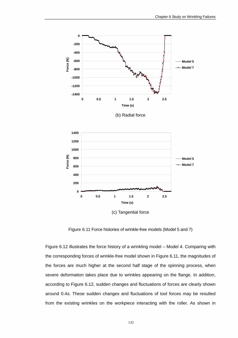
Chapter 6 Study on Wrinkling Failures
132
-1400
-1200
-1000
-800
-600
-400
-200
0
0 0.5 1 1.5 2 2.5
Time (s)
Forc
e (N
)
Model 5
Model 7
(b) Radial force
0
200
400
600
800
1000
1200
1400
0 0.5 1 1.5 2 2.5
Time (s)
Forc
e (N
)
Model 5
Model 7
(c) Tangential force
Figure 6.11 Force histories of wrinkle-free models (Model 5 and 7)
Figure 6.12 illustrates the force history of a wrinkling model – Model 4. Comparing with
the corresponding forces of wrinkle-free model shown in Figure 6.11, the magnitudes of
the forces are much higher at the second half stage of the spinning process, when
severe deformation takes place due to wrinkles appearing on the flange. In addition,
according to Figure 6.12, sudden changes and fluctuations of forces are clearly shown
around 0.4s. These sudden changes and fluctuations of tool forces may be resulted
from the existing wrinkles on the workpiece interacting with the roller. As shown in
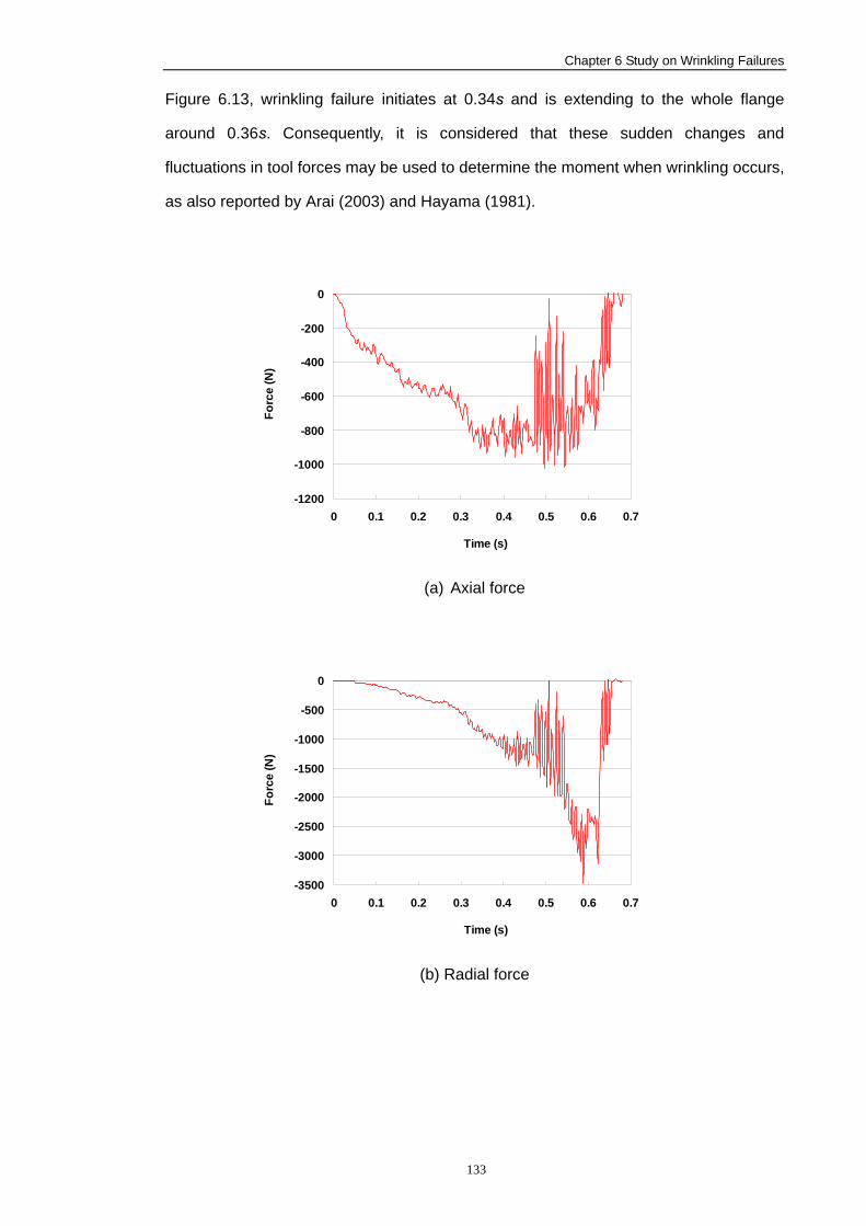
Chapter 6 Study on Wrinkling Failures
133
Figure 6.13, wrinkling failure initiates at 0.34s and is extending to the whole flange
around 0.36s. Consequently, it is considered that these sudden changes and
fluctuations in tool forces may be used to determine the moment when wrinkling occurs,
as also reported by Arai (2003) and Hayama (1981).
-1200
-1000
-800
-600
-400
-200
0
0 0.1 0.2 0.3 0.4 0.5 0.6 0.7
Time (s)
Forc
e (N
)
(a) Axial force
-3500
-3000
-2500
-2000
-1500
-1000
-500
0
0 0.1 0.2 0.3 0.4 0.5 0.6 0.7
Time (s)
Forc
e (N
)
(b) Radial force
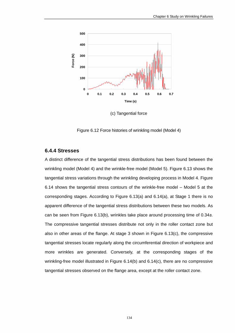
Chapter 6 Study on Wrinkling Failures
134
0
100
200
300
400
500
0 0.1 0.2 0.3 0.4 0.5 0.6 0.7
Time (s)
Forc
e (N
)
(c) Tangential force
Figure 6.12 Force histories of wrinkling model (Model 4)
6.4.4 Stresses A distinct difference of the tangential stress distributions has been found between the
wrinkling model (Model 4) and the wrinkle-free model (Model 5). Figure 6.13 shows the
tangential stress variations through the wrinkling developing process in Model 4. Figure
6.14 shows the tangential stress contours of the wrinkle-free model – Model 5 at the
corresponding stages. According to Figure 6.13(a) and 6.14(a), at Stage 1 there is no
apparent difference of the tangential stress distributions between these two models. As
can be seen from Figure 6.13(b), wrinkles take place around processing time of 0.34s.
The compressive tangential stresses distribute not only in the roller contact zone but
also in other areas of the flange. At stage 3 shown in Figure 6.13(c), the compressive
tangential stresses locate regularly along the circumferential direction of workpiece and
more wrinkles are generated. Conversely, at the corresponding stages of the
wrinkling-free model illustrated in Figure 6.14(b) and 6.14(c), there are no compressive
tangential stresses observed on the flange area, except at the roller contact zone.
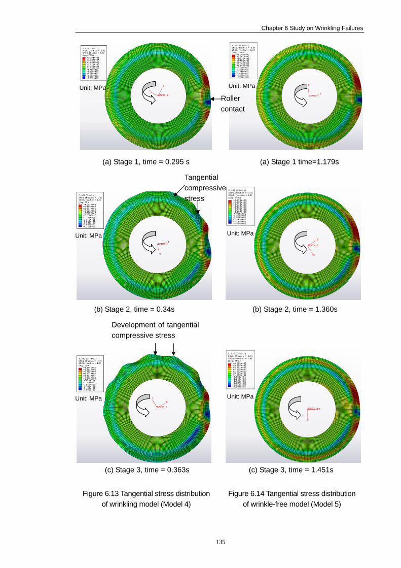
Chapter 6 Study on Wrinkling Failures
135
(a) Stage 1, time = 0.295 s (a) Stage 1 time=1.179s
(b) Stage 2, time = 0.34s (b) Stage 2, time = 1.360s
(c) Stage 3, time = 0.363s (c) Stage 3, time = 1.451s
Figure 6.13 Tangential stress distribution of wrinkling model (Model 4)
Figure 6.14 Tangential stress distribution of wrinkle-free model (Model 5)
Figure 6.14 Tangential stress distribution of wrinkle-free model (Model 5)
Roller contact
Tangential compressive stress
Figure 6.13 Tangential stress distribution of wrinkling model (Model 4)
Development of tangential compressive stress
Unit: MPa
Unit: MPa
Unit: MPa
Unit: MPa
Unit: MPa
Unit: MPa
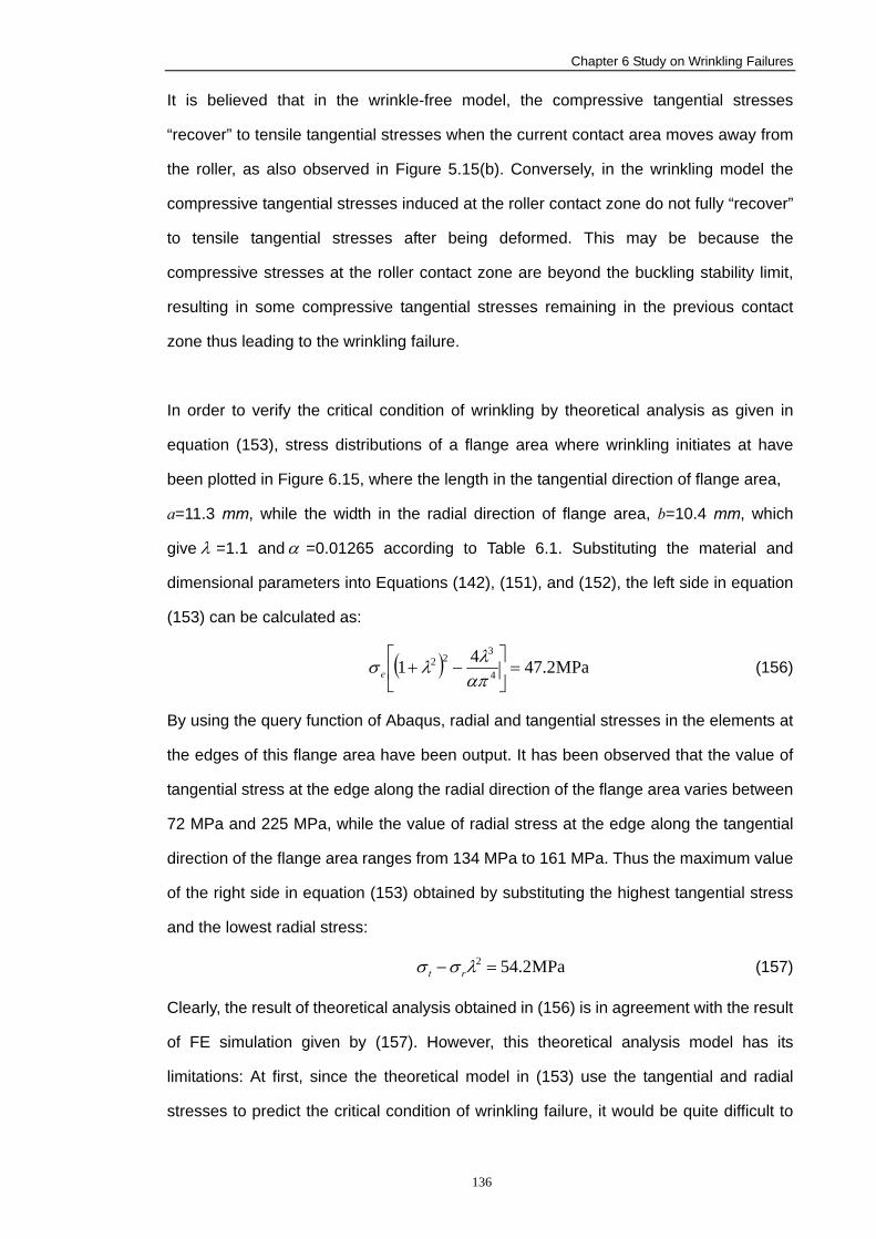
Chapter 6 Study on Wrinkling Failures
136
It is believed that in the wrinkle-free model, the compressive tangential stresses
“recover” to tensile tangential stresses when the current contact area moves away from
the roller, as also observed in Figure 5.15(b). Conversely, in the wrinkling model the
compressive tangential stresses induced at the roller contact zone do not fully “recover”
to tensile tangential stresses after being deformed. This may be because the
compressive stresses at the roller contact zone are beyond the buckling stability limit,
resulting in some compressive tangential stresses remaining in the previous contact
zone thus leading to the wrinkling failure.
In order to verify the critical condition of wrinkling by theoretical analysis as given in
equation (153), stress distributions of a flange area where wrinkling initiates at have
been plotted in Figure 6.15, where the length in the tangential direction of flange area,
a=11.3 mm, while the width in the radial direction of flange area, b=10.4 mm, which
give λ =1.1 andα =0.01265 according to Table 6.1. Substituting the material and
dimensional parameters into Equations (142), (151), and (152), the left side in equation
(153) can be calculated as:
( ) MPa2.4741 4
322 =⎥
⎦
⎤⎢⎣
⎡−+απλλσ e (156)
By using the query function of Abaqus, radial and tangential stresses in the elements at
the edges of this flange area have been output. It has been observed that the value of
tangential stress at the edge along the radial direction of the flange area varies between
72 MPa and 225 MPa, while the value of radial stress at the edge along the tangential
direction of the flange area ranges from 134 MPa to 161 MPa. Thus the maximum value
of the right side in equation (153) obtained by substituting the highest tangential stress
and the lowest radial stress:
MPa2.542 =− λσσ rt (157)
Clearly, the result of theoretical analysis obtained in (156) is in agreement with the result
of FE simulation given by (157). However, this theoretical analysis model has its
limitations: At first, since the theoretical model in (153) use the tangential and radial
stresses to predict the critical condition of wrinkling failure, it would be quite difficult to
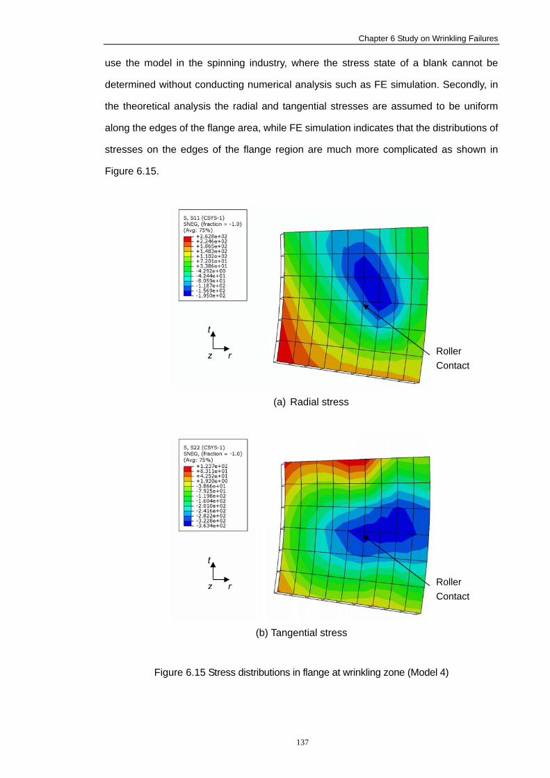
Chapter 6 Study on Wrinkling Failures
137
use the model in the spinning industry, where the stress state of a blank cannot be
determined without conducting numerical analysis such as FE simulation. Secondly, in
the theoretical analysis the radial and tangential stresses are assumed to be uniform
along the edges of the flange area, while FE simulation indicates that the distributions of
stresses on the edges of the flange region are much more complicated as shown in
Figure 6.15.
(a) Radial stress
(b) Tangential stress
Figure 6.15 Stress distributions in flange at wrinkling zone (Model 4)
t
rz
t
rz
Roller Contact
Roller Contact
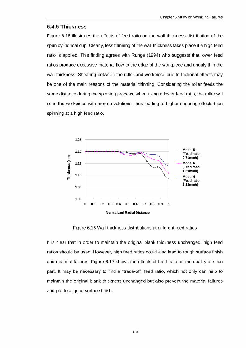
Chapter 6 Study on Wrinkling Failures
138
6.4.5 Thickness Figure 6.16 illustrates the effects of feed ratio on the wall thickness distribution of the
spun cylindrical cup. Clearly, less thinning of the wall thickness takes place if a high feed
ratio is applied. This finding agrees with Runge (1994) who suggests that lower feed
ratios produce excessive material flow to the edge of the workpiece and unduly thin the
wall thickness. Shearing between the roller and workpiece due to frictional effects may
be one of the main reasons of the material thinning. Considering the roller feeds the
same distance during the spinning process, when using a lower feed ratio, the roller will
scan the workpiece with more revolutions, thus leading to higher shearing effects than
spinning at a high feed ratio.
1.00
1.05
1.10
1.15
1.20
1.25
0 0.1 0.2 0.3 0.4 0.5 0.6 0.7 0.8 0.9 1
Normalized Radial Distance
Thic
knes
s (m
m)
Model 5(Feed ratio0.71mm/r)Model 6(Feed ratio1.59mm/r)Model 4(Feed ratio2.12mm/r)
Figure 6.16 Wall thickness distributions at different feed ratios
It is clear that in order to maintain the original blank thickness unchanged, high feed
ratios should be used. However, high feed ratios could also lead to rough surface finish
and material failures. Figure 6.17 shows the effects of feed ratio on the quality of spun
part. It may be necessary to find a “trade-off” feed ratio, which not only can help to
maintain the original blank thickness unchanged but also prevent the material failures
and produce good surface finish.
Chapter 6 Study on Wrinkling Failures
139
Figure 6.17 Effects of feed ratio in blank metal spinning
6.5 Summary and Conclusion
In this chapter, wrinkling failure in conventional spinning has been studied by theoretical
analysis, experimental investigation and Finite Element simulation. The following
conclusions may be drawn:
a) The energy method and two-directional plate buckling theory have been used to
predict the critical condition of wrinkling failure in the conventional spinning.
However, theoretical analysis has shown considerable limitations in comparing with
FE simulation as the stress state of the blank during spinning is far more
complicated than the simplified assumptions made in the theoretical analysis.
b) This study has shown that the reduced integration linear solid element is not
suitable for sheet metal spinning simulation, due to the “hourglassing” problem it
suffered from. Conversely, the reduced integration linear continuum shell element,
which can produce accurate FE analysis results such as wrinkling and tool forces,
should be used to simulate the spinning process.
c) The severity of the wrinkles is quantified by calculating the standard deviation of the
radial coordinates of element nodes on the edge of the spun cup in the FE models.
The results have shown that the severity of the wrinkles increases exponentially
when increasing the feed ratio.
Spindle Speed
High Feed Ratio Zone
Wrinkling Failure
Cracking Failure
High Tool Forces
Low Feed Ratio Zone
Poor Thickness Uniformity
Good Surface Finish
Low Production Efficiency
“Trade-off” Feed
Ratio Zone
Feed Rate
Chapter 6 Study on Wrinkling Failures
140
d) A forming limit study of wrinkling indicates that there is a feed ratio limit beyond
which wrinkling failures will occur. Increasing the feed rate and spindle speed
proportionally, there won’t be much effect on the conventional spinning process.
e) If the high compressive tangential stresses in the local forming zone do not
“recover” to tensile tangential stresses after roller contact, wrinkling failure will
occur.
f) Sudden changes and fluctuations of the tool forces, resulted from existing wrinkles
on the workpiece interacting with the roller, could be used to determine the
approximate moment of wrinkling occurrence.
g) High feed ratios help to maintain the original blank thickness unchanged. However,
high feed ratios also lead to material failures and rough surface finish. It may be
necessary to find a “trade-off” feed ratio zone in the spinning process design.
Chapter 7 Conclusion and Future Work
141
7. Conclusion and Future Work
This chapter summarises the key conclusions on material deformation and wrinkling
failures of conventional spinning drawn from this study. Future research trends of sheet
metal spinning process are also outlined.
7.1 Conclusion
In this study, numerical analysis and experimental investigation have been carried out to
study the material deformation and wrinkling failures in the conventional spinning
process. Key conclusions on six main aspects of this research work are summarised in
the following:
1) Finite Element Simulation
3D elastic-plastic FE simulation of conventional spinning has been carried out under FE
software platform – Abaqus. The computing performances of scaling methods and
element types in the simulation of spinning have been evaluated, respectively. FE
analysis results indicate that both mass scaling and load rate scaling methods with a
suitable scaling factor can produce accurate numerical results, by comparing with a FE
model that does not employ any scaling method. Using a mass scaling factor of f 2 or a
load rate scaling factor of f would speed up the spinning FE simulation by a factor of f. In
addition, FE analysis results also illustrate that the reduced integration linear solid
element is not suitable for the metal spinning simulation, due to the “hourglassing”
problem it suffered from. Conversely, it is believed that the reduced integration linear
continuum shell element, which can produce accurate FE analysis results such as
wrinkling and tool forces, should be used to simulate the sheet metal spinning process.
2) Experiment Investigation
In order to make the workpiece conform to the nonlinear profile of the mandrel, the tool
compensation technique has been investigated and applied in the process of designing
Chapter 7 Conclusion and Future Work
142
multiple roller passes. The tool compensation method is developed based on the
geometry relationship between the roller and the round part of mandrel, when using a
roller to trace the mandrel contour. It has been reported that without taking tool
compensation into account, wrinkling failures may take place on the workpiece due to
unsupported flange. In addition, The Taguchi method has been used to design the
experiment and to study the effects of process parameters on the dimensional variations
of experimental samples. Experimental investigation is also employed in the analysis of
wrinkling failures in the conventional spinning process.
3) Theoretical Analysis of Wrinkling
By using the energy method and two-dimensional plate buckling theory, a theoretical
analysis model to predict the critical condition of wrinkling in the conventional spinning
process has been developed. It shows that the radial and tangential stresses at the
critical condition of wrinkling depend on the geometry of the half-wave wrinkled flange
and the material properties of the blank. Nevertheless, theoretical analysis has shown
considerable limitations in comparing with FE simulation as the stress state of the blank
during spinning is far more complicated than the simplified assumptions on the stresses
of the theoretical model.
4) Material Deformation
To gain insight into the material deformation of conventional spinning, variations of tool
forces, stresses, and strains have been analysed numerically. Axial force dominates at
the beginning of the conventional spinning when the workpiece is mainly subjected to
bending. Radial force increases gradually as roller forms workpeice onto mandrel.
Tangential force keeps almost constant during the conventional spinning process and is
the smallest forces among three force components. Stress analysis shows that in the
forward roller pass, high tensile and compressive radial stresses take place behind and
in front of the roller contact. Two pairs of oppositely directed radial bending effects have
been observed in the workpiece. High tensile radial strains and low compressive
tangential strains are also noticed in the FE models.
Chapter 7 Conclusion and Future Work
143
5) Wrinkling Failures
Wrinkling failure in the conventional spinning process has been studied by using both
numerical and experimental approaches. Compressive tangential stresses are
observed at the flange area near the local forming zone but these will change into
tensile tangential stresses after roller contact in the wrinkle-free models. However, if the
compressive tangential stresses do not fully “recover” to tensile tangential stresses,
wrinkling failure will take place. The severity of the wrinkles is quantified by calculating
the standard deviation of the radial coordinates of element nodes on the edge of spun
cup in the FE models. A forming limit study of wrinkling indicates that there is a feed
ratio limit beyond which wrinkling failures will occur. Increasing the feed rate and spindle
speed proportionally, there will not be much effect on the conventional spinning process.
Sudden changes and fluctuations of the tool forces, resulted from existing wrinkles on
the workpiece interacting with the roller, could be used to determine the approximate
moment of wrinkling occurrence.
6) Process Parameters
According to the experimental results analysis by the Taguchi method, the type of
material has the most significant effects on the thickness and depth variations of spun
parts, followed by the spindle speed and the feed rate. Nevertheless, none of these
input factors show significant effects on the diameter variations. Among four different
roller path designs, i.e. combined concave and convex, convex, linear, and concave
curves, the concave roller path produces the highest tool forces, stresses and deduction
of wall thickness. A greater curvature of the concave path, a higher amount of wall
thinning would take place. On the other hand, lowest tool forces, stresses and wall
thinning are obtained when using the convex roller path. Furthermore, it has been
shown that high feed ratios help to maintain the original blank thickness. However, high
feed ratios also lead to material failures and rough surface finish. It is thus necessary to
find a “trade-off” feed ratio zone in the spinning process design.
Chapter 7 Conclusion and Future Work
144
7.2 Future Work
In this section, four future areas of investigation on the sheet metal spinning process are
identified:
a) FE Simulation of Cracking Failures in Spinning
Up to now, there is no research being conducted on the FE simulation of cracking
failures in the conventional spinning process, although cracking failures also
significantly affects the production efficiency and product quality. Hence, it is believed
that applying FE analysis method to predict and prevent cracking failures in the
conventional spinning is beneficial to the industrial spinning process design. Developing
a suitable material damage model, e.g. defining damage initiation criteria and damage
evolution law, may be one of the key aspects in the FE simulation of cracking failures in
the sheet metal spinning process.
b) Experimental Design and Optimisation
To further analyse the effects of process parameters and their interactions on the quality
of spun part, future experimental design of metal spinning should attempt to take more
input factors at various levels into account, such as the tooling parameters shown in
Figure 1.6. In addition, future work by employing the regression modelling or response
surface methods may be essential to predict the relationships amongst process
parameters and optimise the outputs of metal spinning process.
c) Innovation of Sheet Metal Spinning
Metal spinning process is constrained by two features (Music and Allwood, 2011): it can
only produce axially symmetric parts; a dedicated mandrel is required for each part. In
order to break through these limitations, further research works on asymmetric spinning
and spinning using a general purpose mandrel may be essential. This may require to
design spinning machines with new control systems, such as, force feedback control
(Sekiguchi and Arai, 2010) and synchronous control (Shimizu, 2010).

Chapter 7 Conclusion and Future Work
145
d) Theoretical Analysis of Wrinkling Involving Process Parameters
In this study, the tangential and radial stresses in the local forming zone of workpiece
have been used to predict the critical condition of wrinkling failure. However, this
theoretical model is quite difficult to be directly used in the spinning industry, where the
stress state of workpiece cannot be analysed without carrying out numerical analysis
such as FE simulation. Thus, it is of practical importance to develop a theoretical
analysis approach to relate process parameters, for instance, feed rate, spindle speed
and roller path etc, to the critical stress state in the workpiece and thereby to the
wrinkling failure.
Reference
146
Reference ABAQUS ANALYSIS USER’S MANUAL 2008. ver 6.8. ALBERTI, N., CANNIZZARO, L., LO VALVO, E. & MICARI, F. 1989. Analysis of metal
spinning processes by the ADINA code. Computers & Structures, 32, 517-525. ALBERTI, N. & FRATINI, L. 2004. Innovative sheet metal forming processes: numerical
simulations and experimental tests. Journal of Materials Processing Technology, 150, 2-9.
ARAI, H. 2003. Robotic metal spinning-shear spinning using force feedback control. 2003 IEEE International Conference on Robotics and Automation. Taipei, Taiwan.
ARAI, H. 2006. Force-controlled metal spinning machine using linear motors. 2006 IEEE International Conference on Robotics and Automation. Orlando, Florida.
AUER, C., ERDBR GGE, M. & G BEL, R. 2004. Comparison of multivariate methods for robust parameter design in sheet metal spinning. Applied Stochastic Models in Business and Industry, 20, 201-218.
AVITZUR, B., FLOREEN, S., HUCKE, H. H. & RAGONE, D. V. 1959. An investigation of metal spinning: progress report, College of Engineering, Department of Chemical and Metallurgical Engineering, The University of Michigan.
AVITZUR, B. & YANG, C. T. 1960. Analysis of power spinning of cones. Journal of Engineering for Industry - Transactions of ASME, 82, 231–245.
AWISZUS, B. & H RTEL, S. 2011. Numerical simulation of non-circular spinning: a rotationally non-symmetric spinning process. Production Engineering, 1-8.
BAI, Q., YANG, H. & ZHAN, M. 2008. Finite Element modeling of power spinning of thin-walled shell with hoop inner rib. Transactions of Nonferrous Metals Society of China, 18, 6-13.
BELYTSCHKO, T., LIU, W. K., & MORAN B. 2000. Nonlinear Finite Elements for continua and structures, Chichester, John Wiley & Sons Ltd.
BENI, H. R., BENI, Y. T. & BIGLARI, F. R. 2011. An experimental–numerical investigation of a metal spinning process. Proceedings of the Institution of Mechanical Engineers, Part C: Journal of Mechanical Engineering Science, 225, 509-519.
CHEN, M.-D., HSU, R.-Q. & FUH, K.-H. 2005a. An analysis of force distribution in shear spinning of cone. International Journal of Mechanical Sciences, 47, 902-921.
CHEN, M.-D., HSU, R.-Q. & FUH, K.-H. 2005b. Effects of over-roll thickness on cone surface roughness in shear spinning. Journal of Materials Processing Technology, 159, 1-8.
CHEN, M. D., HSU, R. Q. & FUH, K. H. 2001. Forecast of shear spinning force and surface roughness of spun cones by employing regression analysis. International Journal of Machine Tools and Manufacture, 41, 1721-1734.
CHU, E. & XU, Y. 2001. An elastoplastic analysis of flange wrinkling in deep drawing process. International Journal of Mechanical Sciences, 43, 1421-1440.
DUNNE, F. & PETRINIC, N. 2005. Introduction to computational plasticity, Oxford University Press.
Reference
147
EL-KHABEERY, M. M., FATTOUH, M., EL-SHEIKH, M. N. & HAMED, O. A. 1991. On the conventional simple spinning of cylindrical aluminium cups. International Journal of Machine Tools and Manufacture, 31, 203-219.
ESSA, K. & HARTLEY, P. 2009. Numerical simulation of single and dual pass conventional spinning processes. International Journal of Material Forming, 2, 271-281.
ESSA, K. & HARTLEY, P. 2010. Optimization of conventional spinning process parameters by means of numerical simulation and statistical analysis. Proceedings of the Institution of Mechanical Engineers, Part B: Journal of Engineering Manufacture, 224, 1691-1705.
FILIP, A. C. & NEAGO, I. 2010. Simulation of the metal spinning process by multi-pass path using AutoCAD/VisualLISP. Proc. of 3rd WSEAS International Conference on Engineering Mechanics, Structures, Engineering Geology (EMESEG '10). Corfu Island, Greece.
FOWLKES, W. Y. & CREVELING, C. M. 1995. Engineering methods for robust product design: using Taguchi methods in technology and product development, Addison-Wesley.
GERE, J. M. 2001. Mechanics of materials, Pacific Grove, CA, Brooks/Cole. HAGAN, E. & JESWIET, J. 2003. A review of conventional and modern single-point
sheet metal forming methods. Proceedings of the Institution of Mechanical Engineers, Part B: Journal of Engineering Manufacture, 217, 213-225.
HAMILTON, S. & LONG, H. 2008. Analysis of conventional spinning process of a cylindrical part using finite element method. Steel Research International, Verlag Stahleisen GmbH, 79, 632-639.
HAREWOOD, F. J. & MCHUGH, P. E. 2007. Comparison of the implicit and explicit finite element methods using crystal plasticity. Computational Materials Science, 39, 481-494.
HAYAMA, M. 1981. Study on spinnability of aluminium and its alloys. Bulletin of Faculty of Engineering, Yokohama National University, 30, 63-72.
HAYAMA, M., KUDO, H. & SHINOKURA, T. 1970. Study of the pass schedule in conventional simple spinning. Bulletin of JSME, 13, 1358-1365.
HAYAMA, M. & MUROTA, T. 1963. On the study of metal spinning. Bulletin of Faculty of Engineering, Yokohama National University, 12, 53–88.
HAYAMA, M., MUROTA, T. & KUDO, H. 1965. Experimental study of shear spinning. Bulletin of JSME, 8, 453-460.
HAYAMA, M., MUROTA, T. & KUDO, H. 1966. Deformation modes and wrinkling of flange on shear spinning. Bulletin of JSME, 9, 423-433.
HAYAMA, M. & TAGO, A. 1968. The fracture of walls on shear spinning - study on the spinnability of aluminium plates. Bulletin of Faculty of Engineering, Yokohama National University, 17, 93-103.
HUTCHINSON, J. W. & NEALE, K. W. 1985. Wrinkling of curved thin sheet metal. Plastic Instability, 71-78.
JACKSON, K. & ALLWOOD, J. 2009. The mechanics of incremental sheet forming. Journal of Materials Processing Technology, 209, 1158-1174.
JAGGER, P. 2010. Tool force measurements in the metal spinning process MEng Dissertation, School of Engineering and Computing Sciences, Durham
Reference
148
University. JOSHI, A. M. 2002. Strain studies in sheet metal stampings [Online]. Available:
http://www.metalwebnews.com/howto/sheet-metal/sheetmetal-study.pdf[Accessed February 2011].
JURKOVIC, M., JURKOVIC, Z. & MAHMIC, M. 2006. An analysis and modelling of spinning process without wall-thickness reduction. METABK, 45, 307-312.
KALPAKCIOGLU, S. 1961a. On the mechanics of shear spinning. Journal of Engineering for Industry - Transactions of ASME, 83, 125–130.
KALPAKCIOGLU, S. 1961b. A study of shear-spinability of metals. Journal of Engineering for Industry - Transactions of ASME, 83, 478-484.
KALPAKJIAN, S. & SCHMID, S. 2001. Manufacturing, engineering & technology, London, Prentice Hall.
KANG, D.-C., GAO, X.-C., MENG, X.-F. & WANG, Z.-H. 1999. Study on the deformation mode of conventional spinning of plates. Journal of Materials Processing Technology, 91, 226-230.
KAWAI, K. & HAYAMA, M. 1987. Roller pass programming in conventional spinning by NC spinning machine. Advanced Technology of Plasticity, 11, 711-718.
KAWAI, K., YANG, L. N. & KUDO, H. 2007. A flexible shear spinning of axi-symmetrical shells with a general-purpose mandrel. Journal of Materials Processing Technology, 192-193, 13-17.
KEGG, R. 1961. A new test method for determination of spinnability of metals. Journal of Engineering for Industry - Transactions of ASME, 83, 118-125.
KIM, J., PARK, J. & KIM, C. 2006. A study on the mechanics of shear spinning of cones. Journal of Mechanical Science and Technology, 20, 806-818.
KLEINER, M., EWERS, R., KUNERT, J., HENKENJOHANN, N. & AUER, C. 2005. Optimisation of the shear forming process by means of multivariate statistical methods[Online].Available:http://www.statistik.tu-dortmund.de/fileadmin/user_upload/Lehrstuehle/MSind/SFB_475/2005/tr23-05.pdf [Accessed February 2011].
KLEINER, M., G BEL, R., KANTZ, H., KLIMMEK, C. & HOMBERG, W. 2002. Combined methods for the prediction of dynamic instabilities in sheet metal spinning. CIRP Annals - Manufacturing Technology, 51, 209-214.
KLIMMEK, C., GOBEL, R., HOMBERG, W., KANTZ, H. & KLEINER, M. 2002. Finite element analysis of sheet metal forming by spinning. Proc. of 7th International Conference on Technology of Plasticity. Yokohama, Japan.
KOBAYASHI, S. 1963. Instability in conventional spinning of cones. Journal of Engineering for Industry - Transactions of ASME, 85, 44-48.
KOBAYASHI, S., HALL, I. K. & THOMSEN, E. G. 1961. A theory of shear spinning of cones. Journal of Engineering for Industry, 83, 485-495.
LEE, K. S. & NOBLE, C. F. 1982. The effect of relative angle between work and roller axes on forces and material characteristics in flow turning of aluminium cones. Proc. of 2nd International Conference on Rotary Metal-Working Processes. Stratford upon Avon, UK.
LIU, C.-H. 2007. The simulation of the multi-pass and die-less spinning process. Journal of Materials Processing Technology, 192-193, 518-524.
LIU, J. H., YANG, H. & LI, Y. Q. 2002. A study of the stress and strain distributions of first-pass conventional spinning under different roller-traces. Journal of Materials
Reference
149
Processing Technology, 129, 326-329. LIU, G. R. & QUEK, S. S. 2003. The Finite Element method: a practical course, Oxford,
Butterworth-Heinemann. LONG, H. & HAMILTON, S. 2008. Simulation of effects of material deformation on
thickness variation in conventional spinning. Proc. of 9th International Conference on Technology of Plasticity. Kyeongju, South Korea.
LONG, H., WANG, L. & JAGGER, P. 2011. Roller force analysis in multi-pass conventional spinning by finite element simulation and experimental measurement. The 10th International Conference on Technology of Plasticity. Aachen, Germany.
LU, X., ZHANG, S., HOU, H., LI, J., ZHOU, L. & LI, Z. 2006. Three dimensional FE analysis on flange bending for TC4 alloy during shear spinning. Journal of Materials Science and Technology, 22, 855-859.
MA, F., YANG, H. & ZHAN, M. 2010. Plastic deformation behaviors and their application in power spinning process of conical parts with transverse inner rib. Journal of Materials Processing Technology, 210, 180-189.
MONTGOMERY, D. C. 2009. Design and analysis of experiments, John Wiley & Sons (Asia)
MORI, K.-I. & NONAKA, T. 2005. Simplified three-dimensional finite element simulation of shear spinning process based on axisymmetric modeling. Journal of Manufacturing Processes, 7, 51-56.
MUSIC, O. & ALLWOOD, J. M. 2011. Flexible asymmetric spinning. CIRP Annals - Manufacturing Technology, In Press, Corrected Proof.
MUSIC, O., ALLWOOD, J. M. & KAWAI, K. 2010. A review of the mechanics of metal spinning. Journal of Materials Processing Technology, 210, 3-23.
OZER, A. & ARAI, H. 2009. Robotic metal spinning-experimental implementation using an industrial robot arm. 2009 IEEE International Conference on Robotics and Automation. Kobe, Japan.
PELL, S. 2009. Simulation of the metal spinning process. MEng Dissertation, School of Engineering and Computing Sciences, Durham University
PEREZ, A., GARC A, J. & FRANCISCO, P. 1984. A study about parameters influence in shear spinning. Proc. of 3rd International Conference on Rotary Metal-Working Processes. Kyoto, Japan.
POLLITT, D. H. 1982. The development of a new playback or skill recording control system for metal spinning Proc. of 2nd International Conference on Rotary Metal-Working Processes. Stratford upon Avon, UK.
QUIGLEY, E. & MONAGHAN, J. 1999. An analysis of conventional spinning of light sheet metal. International Conference on Sheet Metal. Erlangen, Germany.
QUIGLEY, E. & MONAGHAN, J. 2000. Metal forming: an analysis of spinning processes. Journal of Materials Processing Technology, 103, 114-119.
QUIGLEY, E. & MONAGHAN, J. 2002a. Enhanced finite element models of metal spinning. Journal of Materials Processing Technology, 121, 43-49.
QUIGLEY, E. & MONAGHAN, J. 2002b. The finite element modelling of conventional spinning using multi-domain models. Journal of Materials Processing Technology, 124, 360-365.
RAO, S. S. 2005. The Finite Element method in engineering. Burlington,
Reference
150
Butterworth-Heinemann. RAZAVI, H., BIGLARI, F. R. & TORABKHANI, A. 2005. Study of strains distribution in
spinning process using FE simulation and experimental work. Tehran International Congress on Manufacturing Engineering (TICME2005). Tehran, Iran.
REITMANN, V. & KANTZ, H. 2001. Plastic wrinkling and flutter in sheet metal spinning [Online]. Available: http://www.vreitmann.de/reitmann/wrinkling.html [Accessed 15 February 2011].
RUNGE, M. 1994. Spinning and flow forming (Pollitt, D. H. Trans), Leifield GmbH. SATOH, T. & YANAGIMOTO, S. 1982. On the spinnability of steel sheets. Proc. of 2nd
International Conference on Rotary Metal-Working Processes. Stratford upon Avon, UK.
SEBASTIANI, G., BROSIUS, A., EWERS, R., KLEINER, M. & KLIMMEK, C. 2006. Numerical investigation on dynamic effects during sheet metal spinning by explicit finite-element-analysis. Journal of Materials Processing Technology, 177, 401-403.
SEBASTIANI, G., BROSIUS, A., HOMBERG, W. & KLEINER, M. 2007. Process characterization of sheet metal spinning by means of Finite Elements. Key Engineering Materials, 334, 637-644.
SEKIGUCHI, A. & ARAI, H. 2010. Synchronous die-less spinning of curved products. Steel Research International, 81, 1010-1013.
SENIOR, B. W. 1956. Flange wrinkling in deep-drawing operations. Journal of Mechanics and Physics of Solids, 4, 235-246.
SHIMIZU, I. 2010. Asymmetric forming of aluminum sheets by synchronous spinning. Journal of Materials Processing Technology, 210, 585-592.
SLATER, R. A. C. 1979a. The effects of mandrel speed and roller feed rate on the external surface finish during the spin-forging of 70/30 brass sheet metal cones Proc. of 1st International Conference on Rotary Metal-Working Processes. London, UK.
SLATER, R. A. C. 1979b. A review of analytical and experimental investigations of the spin-forging of sheet metal cones. Proc. of 1st International Conference on Rotary Metal-Working Processes. London, UK.
SORTAIS, H. C., KOBAYASHI, S. & THOMSEN, E. G. 1963. Mechanics of conventional spinning. Journal of Engineering for Industry - Transactions of ASME, 85, 346–350.
TEKKAYA, A. E. 2000. State-of-the-art of simulation of sheet metal forming. Journal of Materials Processing Technology, 103, 14-22.
TIMOSHENKO, S. 1936. Theory of elastic stability, New York ; London, McGraw-Hill Book Company, inc.
TIMOSHENKO, S. & WOINOWSKY-KRIEGER, S. 1959. Theory of plates and shells, New York, McGraw-Hill book company.
WANG, L. 2005. Finite Element Analysis of C64 Railway Vehicle. BEng Thesis, Dalian Jiaotong University.
WANG, L. & LONG, H. 2010. Stress analysis of multi-pass conventional spinning. Proc. of 8th International Conference on Manufacturing Research. Durham, UK.
WANG, L. & LONG, H. 2011a. Investigation of effects of roller path profiles on wrinkling
Reference
151
in conventional spinning. The 10th International Conference on Technology of Plasticity. Aachen, Germany.
WANG, L. & LONG, H. 2011b. Investigation of material deformation in multi-pass conventional metal spinning. Materials & Design, 32, 2891-2899.
WANG, L. & LONG, H. 2011c. A study of effects of roller path profiles on tool forces and part wall thickness variation in conventional metal spinning. Journal of Materials Processing Technology, 211, 2140-2151.
WANG, L., LONG, H., ASHLEY, D., ROBERTS, M. & WHITE, P. 2010. Analysis of single-pass conventional spinning by Taguchi and finite element methods. Steel Research International, 81, 974-977.
WANG, L., LONG, H., ASHLEY, D., ROBERTS, M. & WHITE, P. 2011. Effects of roller feed ratio on wrinkling failure in conventional spinning of a cylindrical cup. Proceedings of the Institution of Mechanical Engineers, Part B, Journal of Engineering Manufacture, 225, 1991-2006.
WANG, Q., WANG, T. & WANG, Z. R. 1989. A study of the working force in conventional spinning. Proc. of 4th International Conference on Rotary Forming. Beijing, China.
WANG, X. & CAO, J. 2000. An Analytical Prediction of Flange Wrinkling in Sheet Metal Forming. Journal of Manufacturing Processes, 2, 100-107.
WICK, C., BENEDICT, J. T. & VEILLEUX, R. F. 1984. Tool and Manufacturing Engineers Handbook, Michigan, USA, Society of Manufacturing Engineers.
WILSON, J. S. 2005. Sensor technology handbook Oxford, Newnes. WONG, C. C., DEAN, T. A. & LIN, J. 2003. A review of spinning, shear forming and flow
forming processes. International Journal of Machine Tools and Manufacture, 43, 1419-1435.
XIA, Q., SHIMA, S., KOTERA, H. & YASUHUKU, D. 2005. A study of the one-path deep drawing spinning of cups. Journal of Materials Processing Technology, 159, 397-400.
YOUNGER, A. 1979. The effect of roller tool profile on the tool forces in hydraulic metal spinning. Proc. of 1st International Conference on Rotary Metal-Working Processes. London, UK.
ZHAN, M., YANG, H., JIANG, Z. Q. & ZHANG, J. H. 2008. 3D FEM analysis of forming parameters on cone spinning based on orthogonal experimental design method. Proc. of 9th International Conference on Technology of Plasticity. Kyeongju, South Korea
ZHAN, M., YANG, H., ZHANG, J. H., XU, Y. L. & MA, F. 2007. 3D FEM analysis of influence of roller feed rate on forming force and quality of cone spinning. Journal of Materials Processing Technology, 187-188, 486-491.
ZHANG, S.-H., LU, X.-Y., LIU, H., HOU, H.-L., LI, Z.-Q. & ZENG, Y.-S. 2010. Effects of feeding ratio on flange bending in shear spinning. International Journal of Material Forming, 1-7.
ZHAO, J.-H., CHAMPLIAUD, H. & DAO, T.-M. 2007. Simulation of shear spinning process using finite element method. Proc. of 18th IASTED International Conference: Modelling and Simulation. Montreal, Canada.
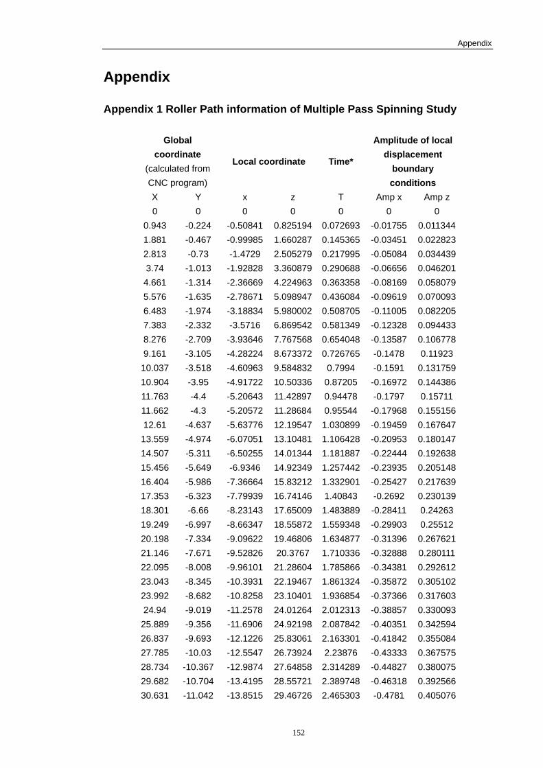
Appendix
152
Appendix
Appendix 1 Roller Path information of Multiple Pass Spinning Study
Global coordinate
(calculated from CNC program)
Local coordinate Time*
Amplitude of local displacement
boundary conditions
X Y x z T Amp x Amp z 0 0 0 0 0 0 0
0.943 -0.224 -0.50841 0.825194 0.072693 -0.01755 0.0113441.881 -0.467 -0.99985 1.660287 0.145365 -0.03451 0.0228232.813 -0.73 -1.4729 2.505279 0.217995 -0.05084 0.0344393.74 -1.013 -1.92828 3.360879 0.290688 -0.06656 0.0462014.661 -1.314 -2.36669 4.224963 0.363358 -0.08169 0.0580795.576 -1.635 -2.78671 5.098947 0.436084 -0.09619 0.0700936.483 -1.974 -3.18834 5.980002 0.508705 -0.11005 0.0822057.383 -2.332 -3.5716 6.869542 0.581349 -0.12328 0.0944338.276 -2.709 -3.93646 7.767568 0.654048 -0.13587 0.1067789.161 -3.105 -4.28224 8.673372 0.726765 -0.1478 0.11923
10.037 -3.518 -4.60963 9.584832 0.7994 -0.1591 0.13175910.904 -3.95 -4.91722 10.50336 0.87205 -0.16972 0.14438611.763 -4.4 -5.20643 11.42897 0.94478 -0.1797 0.1571111.662 -4.3 -5.20572 11.28684 0.95544 -0.17968 0.15515612.61 -4.637 -5.63776 12.19547 1.030899 -0.19459 0.167647
13.559 -4.974 -6.07051 13.10481 1.106428 -0.20953 0.18014714.507 -5.311 -6.50255 14.01344 1.181887 -0.22444 0.19263815.456 -5.649 -6.9346 14.92349 1.257442 -0.23935 0.20514816.404 -5.986 -7.36664 15.83212 1.332901 -0.25427 0.21763917.353 -6.323 -7.79939 16.74146 1.40843 -0.2692 0.23013918.301 -6.66 -8.23143 17.65009 1.483889 -0.28411 0.2426319.249 -6.997 -8.66347 18.55872 1.559348 -0.29903 0.2551220.198 -7.334 -9.09622 19.46806 1.634877 -0.31396 0.26762121.146 -7.671 -9.52826 20.3767 1.710336 -0.32888 0.28011122.095 -8.008 -9.96101 21.28604 1.785866 -0.34381 0.29261223.043 -8.345 -10.3931 22.19467 1.861324 -0.35872 0.30510223.992 -8.682 -10.8258 23.10401 1.936854 -0.37366 0.31760324.94 -9.019 -11.2578 24.01264 2.012313 -0.38857 0.330093
25.889 -9.356 -11.6906 24.92198 2.087842 -0.40351 0.34259426.837 -9.693 -12.1226 25.83061 2.163301 -0.41842 0.35508427.785 -10.03 -12.5547 26.73924 2.23876 -0.43333 0.36757528.734 -10.367 -12.9874 27.64858 2.314289 -0.44827 0.38007529.682 -10.704 -13.4195 28.55721 2.389748 -0.46318 0.39256630.631 -11.042 -13.8515 29.46726 2.465303 -0.4781 0.405076
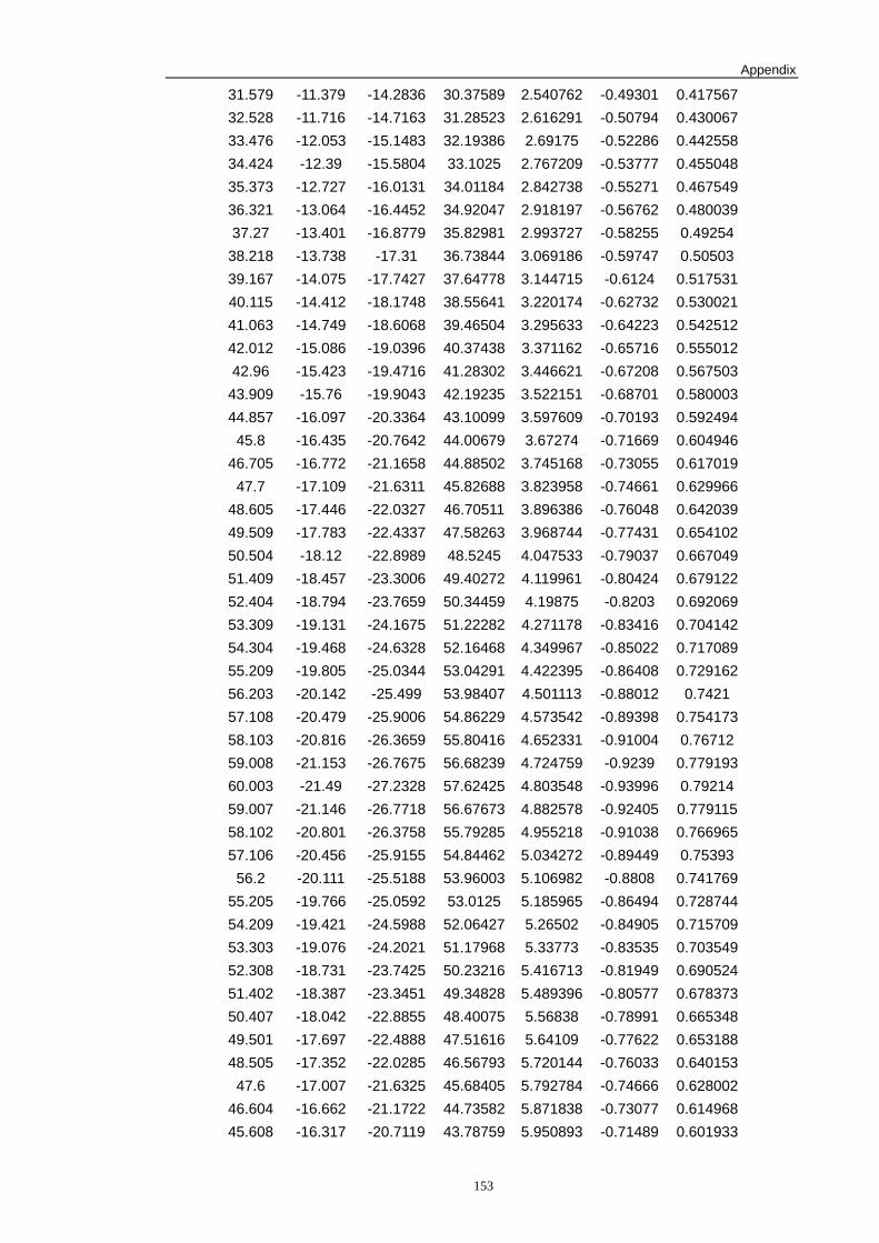
Appendix
153
31.579 -11.379 -14.2836 30.37589 2.540762 -0.49301 0.41756732.528 -11.716 -14.7163 31.28523 2.616291 -0.50794 0.43006733.476 -12.053 -15.1483 32.19386 2.69175 -0.52286 0.44255834.424 -12.39 -15.5804 33.1025 2.767209 -0.53777 0.45504835.373 -12.727 -16.0131 34.01184 2.842738 -0.55271 0.46754936.321 -13.064 -16.4452 34.92047 2.918197 -0.56762 0.48003937.27 -13.401 -16.8779 35.82981 2.993727 -0.58255 0.49254
38.218 -13.738 -17.31 36.73844 3.069186 -0.59747 0.5050339.167 -14.075 -17.7427 37.64778 3.144715 -0.6124 0.51753140.115 -14.412 -18.1748 38.55641 3.220174 -0.62732 0.53002141.063 -14.749 -18.6068 39.46504 3.295633 -0.64223 0.54251242.012 -15.086 -19.0396 40.37438 3.371162 -0.65716 0.55501242.96 -15.423 -19.4716 41.28302 3.446621 -0.67208 0.567503
43.909 -15.76 -19.9043 42.19235 3.522151 -0.68701 0.58000344.857 -16.097 -20.3364 43.10099 3.597609 -0.70193 0.592494
45.8 -16.435 -20.7642 44.00679 3.67274 -0.71669 0.60494646.705 -16.772 -21.1658 44.88502 3.745168 -0.73055 0.617019
47.7 -17.109 -21.6311 45.82688 3.823958 -0.74661 0.62996648.605 -17.446 -22.0327 46.70511 3.896386 -0.76048 0.64203949.509 -17.783 -22.4337 47.58263 3.968744 -0.77431 0.65410250.504 -18.12 -22.8989 48.5245 4.047533 -0.79037 0.66704951.409 -18.457 -23.3006 49.40272 4.119961 -0.80424 0.67912252.404 -18.794 -23.7659 50.34459 4.19875 -0.8203 0.69206953.309 -19.131 -24.1675 51.22282 4.271178 -0.83416 0.70414254.304 -19.468 -24.6328 52.16468 4.349967 -0.85022 0.71708955.209 -19.805 -25.0344 53.04291 4.422395 -0.86408 0.72916256.203 -20.142 -25.499 53.98407 4.501113 -0.88012 0.7421 57.108 -20.479 -25.9006 54.86229 4.573542 -0.89398 0.75417358.103 -20.816 -26.3659 55.80416 4.652331 -0.91004 0.7671259.008 -21.153 -26.7675 56.68239 4.724759 -0.9239 0.77919360.003 -21.49 -27.2328 57.62425 4.803548 -0.93996 0.7921459.007 -21.146 -26.7718 56.67673 4.882578 -0.92405 0.77911558.102 -20.801 -26.3758 55.79285 4.955218 -0.91038 0.76696557.106 -20.456 -25.9155 54.84462 5.034272 -0.89449 0.75393
56.2 -20.111 -25.5188 53.96003 5.106982 -0.8808 0.74176955.205 -19.766 -25.0592 53.0125 5.185965 -0.86494 0.72874454.209 -19.421 -24.5988 52.06427 5.26502 -0.84905 0.71570953.303 -19.076 -24.2021 51.17968 5.33773 -0.83535 0.70354952.308 -18.731 -23.7425 50.23216 5.416713 -0.81949 0.69052451.402 -18.387 -23.3451 49.34828 5.489396 -0.80577 0.67837350.407 -18.042 -22.8855 48.40075 5.56838 -0.78991 0.66534849.501 -17.697 -22.4888 47.51616 5.64109 -0.77622 0.65318848.505 -17.352 -22.0285 46.56793 5.720144 -0.76033 0.640153
47.6 -17.007 -21.6325 45.68405 5.792784 -0.74666 0.62800246.604 -16.662 -21.1722 44.73582 5.871838 -0.73077 0.61496845.608 -16.317 -20.7119 43.78759 5.950893 -0.71489 0.601933
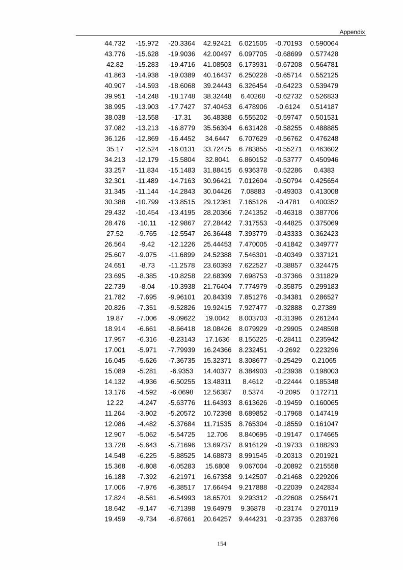
Appendix
154
44.732 -15.972 -20.3364 42.92421 6.021505 -0.70193 0.59006443.776 -15.628 -19.9036 42.00497 6.097705 -0.68699 0.57742842.82 -15.283 -19.4716 41.08503 6.173931 -0.67208 0.564781
41.863 -14.938 -19.0389 40.16437 6.250228 -0.65714 0.55212540.907 -14.593 -18.6068 39.24443 6.326454 -0.64223 0.53947939.951 -14.248 -18.1748 38.32448 6.40268 -0.62732 0.52683338.995 -13.903 -17.7427 37.40453 6.478906 -0.6124 0.51418738.038 -13.558 -17.31 36.48388 6.555202 -0.59747 0.50153137.082 -13.213 -16.8779 35.56394 6.631428 -0.58255 0.48888536.126 -12.869 -16.4452 34.6447 6.707629 -0.56762 0.47624835.17 -12.524 -16.0131 33.72475 6.783855 -0.55271 0.463602
34.213 -12.179 -15.5804 32.8041 6.860152 -0.53777 0.45094633.257 -11.834 -15.1483 31.88415 6.936378 -0.52286 0.4383 32.301 -11.489 -14.7163 30.96421 7.012604 -0.50794 0.42565431.345 -11.144 -14.2843 30.04426 7.08883 -0.49303 0.41300830.388 -10.799 -13.8515 29.12361 7.165126 -0.4781 0.40035229.432 -10.454 -13.4195 28.20366 7.241352 -0.46318 0.38770628.476 -10.11 -12.9867 27.28442 7.317553 -0.44825 0.37506927.52 -9.765 -12.5547 26.36448 7.393779 -0.43333 0.362423
26.564 -9.42 -12.1226 25.44453 7.470005 -0.41842 0.34977725.607 -9.075 -11.6899 24.52388 7.546301 -0.40349 0.33712124.651 -8.73 -11.2578 23.60393 7.622527 -0.38857 0.32447523.695 -8.385 -10.8258 22.68399 7.698753 -0.37366 0.31182922.739 -8.04 -10.3938 21.76404 7.774979 -0.35875 0.29918321.782 -7.695 -9.96101 20.84339 7.851276 -0.34381 0.28652720.826 -7.351 -9.52826 19.92415 7.927477 -0.32888 0.2738919.87 -7.006 -9.09622 19.0042 8.003703 -0.31396 0.261244
18.914 -6.661 -8.66418 18.08426 8.079929 -0.29905 0.24859817.957 -6.316 -8.23143 17.1636 8.156225 -0.28411 0.23594217.001 -5.971 -7.79939 16.24366 8.232451 -0.2692 0.22329616.045 -5.626 -7.36735 15.32371 8.308677 -0.25429 0.2106515.089 -5.281 -6.9353 14.40377 8.384903 -0.23938 0.19800314.132 -4.936 -6.50255 13.48311 8.4612 -0.22444 0.18534813.176 -4.592 -6.0698 12.56387 8.5374 -0.2095 0.17271112.22 -4.247 -5.63776 11.64393 8.613626 -0.19459 0.16006511.264 -3.902 -5.20572 10.72398 8.689852 -0.17968 0.14741912.086 -4.482 -5.37684 11.71535 8.765304 -0.18559 0.16104712.907 -5.062 -5.54725 12.706 8.840695 -0.19147 0.17466513.728 -5.643 -5.71696 13.69737 8.916129 -0.19733 0.18829314.548 -6.225 -5.88525 14.68873 8.991545 -0.20313 0.20192115.368 -6.808 -6.05283 15.6808 9.067004 -0.20892 0.21555816.188 -7.392 -6.21971 16.67358 9.142507 -0.21468 0.22920617.006 -7.976 -6.38517 17.66494 9.217888 -0.22039 0.24283417.824 -8.561 -6.54993 18.65701 9.293312 -0.22608 0.25647118.642 -9.147 -6.71398 19.64979 9.36878 -0.23174 0.27011919.459 -9.734 -6.87661 20.64257 9.444231 -0.23735 0.283766
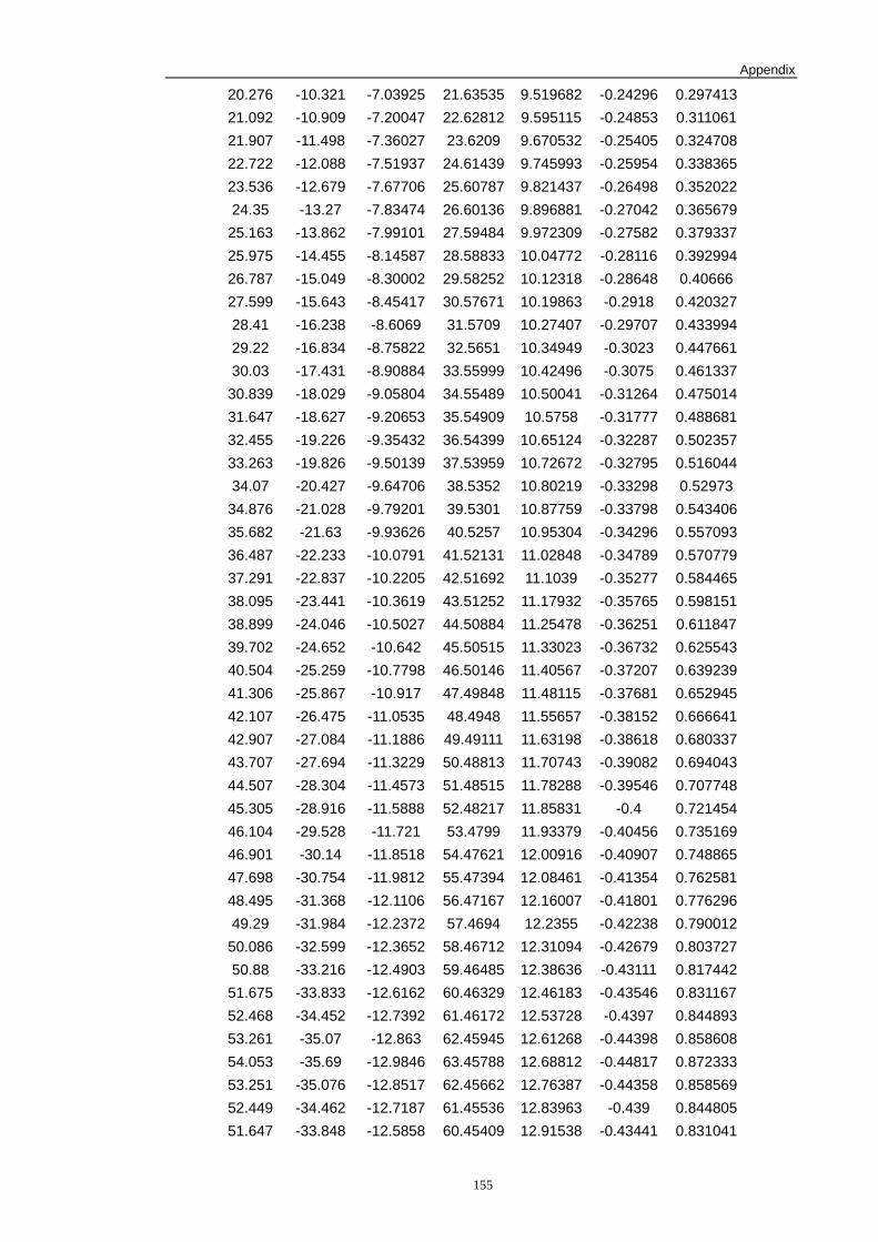
Appendix
155
20.276 -10.321 -7.03925 21.63535 9.519682 -0.24296 0.29741321.092 -10.909 -7.20047 22.62812 9.595115 -0.24853 0.31106121.907 -11.498 -7.36027 23.6209 9.670532 -0.25405 0.32470822.722 -12.088 -7.51937 24.61439 9.745993 -0.25954 0.33836523.536 -12.679 -7.67706 25.60787 9.821437 -0.26498 0.35202224.35 -13.27 -7.83474 26.60136 9.896881 -0.27042 0.365679
25.163 -13.862 -7.99101 27.59484 9.972309 -0.27582 0.37933725.975 -14.455 -8.14587 28.58833 10.04772 -0.28116 0.39299426.787 -15.049 -8.30002 29.58252 10.12318 -0.28648 0.4066627.599 -15.643 -8.45417 30.57671 10.19863 -0.2918 0.42032728.41 -16.238 -8.6069 31.5709 10.27407 -0.29707 0.43399429.22 -16.834 -8.75822 32.5651 10.34949 -0.3023 0.44766130.03 -17.431 -8.90884 33.55999 10.42496 -0.3075 0.461337
30.839 -18.029 -9.05804 34.55489 10.50041 -0.31264 0.47501431.647 -18.627 -9.20653 35.54909 10.5758 -0.31777 0.48868132.455 -19.226 -9.35432 36.54399 10.65124 -0.32287 0.50235733.263 -19.826 -9.50139 37.53959 10.72672 -0.32795 0.51604434.07 -20.427 -9.64706 38.5352 10.80219 -0.33298 0.52973
34.876 -21.028 -9.79201 39.5301 10.87759 -0.33798 0.54340635.682 -21.63 -9.93626 40.5257 10.95304 -0.34296 0.55709336.487 -22.233 -10.0791 41.52131 11.02848 -0.34789 0.57077937.291 -22.837 -10.2205 42.51692 11.1039 -0.35277 0.58446538.095 -23.441 -10.3619 43.51252 11.17932 -0.35765 0.59815138.899 -24.046 -10.5027 44.50884 11.25478 -0.36251 0.61184739.702 -24.652 -10.642 45.50515 11.33023 -0.36732 0.62554340.504 -25.259 -10.7798 46.50146 11.40567 -0.37207 0.63923941.306 -25.867 -10.917 47.49848 11.48115 -0.37681 0.65294542.107 -26.475 -11.0535 48.4948 11.55657 -0.38152 0.66664142.907 -27.084 -11.1886 49.49111 11.63198 -0.38618 0.68033743.707 -27.694 -11.3229 50.48813 11.70743 -0.39082 0.69404344.507 -28.304 -11.4573 51.48515 11.78288 -0.39546 0.70774845.305 -28.916 -11.5888 52.48217 11.85831 -0.4 0.72145446.104 -29.528 -11.721 53.4799 11.93379 -0.40456 0.73516946.901 -30.14 -11.8518 54.47621 12.00916 -0.40907 0.74886547.698 -30.754 -11.9812 55.47394 12.08461 -0.41354 0.76258148.495 -31.368 -12.1106 56.47167 12.16007 -0.41801 0.77629649.29 -31.984 -12.2372 57.4694 12.2355 -0.42238 0.790012
50.086 -32.599 -12.3652 58.46712 12.31094 -0.42679 0.80372750.88 -33.216 -12.4903 59.46485 12.38636 -0.43111 0.817442
51.675 -33.833 -12.6162 60.46329 12.46183 -0.43546 0.83116752.468 -34.452 -12.7392 61.46172 12.53728 -0.4397 0.84489353.261 -35.07 -12.863 62.45945 12.61268 -0.44398 0.85860854.053 -35.69 -12.9846 63.45788 12.68812 -0.44817 0.87233353.251 -35.076 -12.8517 62.45662 12.76387 -0.44358 0.85856952.449 -34.462 -12.7187 61.45536 12.83963 -0.439 0.84480551.647 -33.848 -12.5858 60.45409 12.91538 -0.43441 0.831041
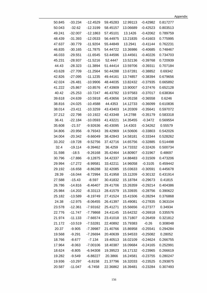
Appendix
156
50.845 -33.234 -12.4529 59.45283 12.99113 -0.42982 0.81727750.043 -32.62 -12.3199 58.45157 13.06689 -0.42523 0.80351349.241 -32.007 -12.1863 57.45101 13.1426 -0.42062 0.78975948.439 -31.393 -12.0533 56.44975 13.21835 -0.41603 0.77599547.637 -30.779 -11.9204 55.44849 13.2941 -0.41144 0.76223146.835 -30.165 -11.7875 54.44722 13.36986 -0.40685 0.74846746.033 -29.551 -11.6545 53.44596 13.44561 -0.40226 0.73470345.231 -28.937 -11.5216 52.4447 13.52136 -0.39768 0.72093944.43 -28.323 -11.3894 51.44414 13.59706 -0.39311 0.707184
43.628 -27.709 -11.2564 50.44288 13.67281 -0.38852 0.6934242.826 -27.095 -11.1235 49.44161 13.74857 -0.38394 0.67965642.024 -26.481 -10.9906 48.44035 13.82432 -0.37935 0.66589241.222 -25.867 -10.8576 47.43909 13.90007 -0.37476 0.65212840.42 -25.253 -10.7247 46.43782 13.97583 -0.37017 0.638364
39.618 -24.639 -10.5918 45.43656 14.05158 -0.36558 0.6246 38.816 -24.025 -10.4588 44.4353 14.12733 -0.36099 0.61083638.014 -23.411 -10.3259 43.43403 14.20309 -0.35641 0.59707237.212 -22.798 -10.1922 42.43348 14.2788 -0.35179 0.58331836.41 -22.184 -10.0593 41.43221 14.35455 -0.3472 0.569554
35.608 -21.57 -9.92636 40.43095 14.4303 -0.34262 0.5557934.806 -20.956 -9.79343 39.42969 14.50606 -0.33803 0.54202634.004 -20.342 -9.66049 38.42843 14.58181 -0.33344 0.52826233.202 -19.728 -9.52756 37.42716 14.65756 -0.32885 0.514498
32.4 -19.114 -9.39462 36.4259 14.73332 -0.32426 0.50073431.598 -18.5 -9.26168 35.42464 14.80907 -0.31967 0.4869730.796 -17.886 -9.12875 34.42337 14.88483 -0.31509 0.47320629.994 -17.272 -8.99581 33.42211 14.96058 -0.3105 0.45944229.192 -16.658 -8.86288 32.42085 15.03633 -0.30591 0.44567828.39 -16.044 -8.72994 31.41958 15.11209 -0.30132 0.431914
27.588 -15.43 -8.597 30.41832 15.18784 -0.29673 0.4181526.786 -14.816 -8.46407 29.41706 15.26359 -0.29214 0.40438625.984 -14.202 -8.33113 28.41579 15.33935 -0.28756 0.39062225.182 -13.589 -8.19749 27.41524 15.41506 -0.28294 0.37686824.38 -12.975 -8.06455 26.41397 15.49081 -0.27835 0.363104
23.578 -12.361 -7.93162 25.41271 15.56656 -0.27377 0.3493422.776 -11.747 -7.79868 24.41145 15.64232 -0.26918 0.33557621.974 -11.133 -7.66574 23.41018 15.71807 -0.26459 0.32181221.172 -10.519 -7.53281 22.40892 15.79383 -0.26 0.30804820.37 -9.905 -7.39987 21.40766 15.86958 -0.25541 0.294284
19.568 -9.291 -7.26694 20.40639 15.94533 -0.25082 0.2805218.766 -8.677 -7.134 19.40513 16.02109 -0.24624 0.26675517.964 -8.063 -7.00106 18.40387 16.09684 -0.24165 0.25299118.624 -8.805 -6.94308 19.39523 16.17132 -0.23965 0.26661919.282 -9.549 -6.88227 20.3866 16.24581 -0.23755 0.28024719.936 -10.297 -6.8158 21.37796 16.32033 -0.23525 0.29387520.587 -11.047 -6.7458 22.36862 16.39481 -0.23284 0.307493
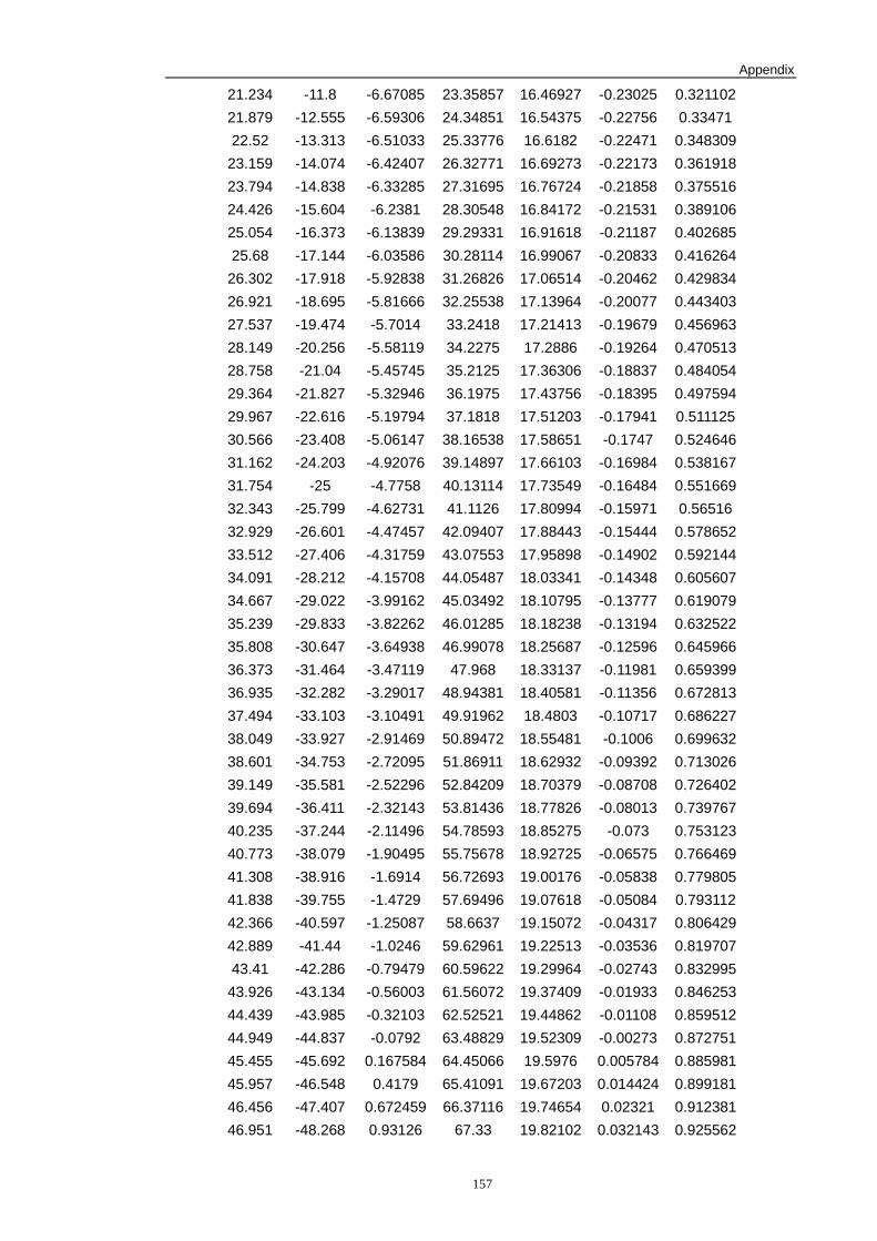
Appendix
157
21.234 -11.8 -6.67085 23.35857 16.46927 -0.23025 0.32110221.879 -12.555 -6.59306 24.34851 16.54375 -0.22756 0.3347122.52 -13.313 -6.51033 25.33776 16.6182 -0.22471 0.348309
23.159 -14.074 -6.42407 26.32771 16.69273 -0.22173 0.36191823.794 -14.838 -6.33285 27.31695 16.76724 -0.21858 0.37551624.426 -15.604 -6.2381 28.30548 16.84172 -0.21531 0.38910625.054 -16.373 -6.13839 29.29331 16.91618 -0.21187 0.40268525.68 -17.144 -6.03586 30.28114 16.99067 -0.20833 0.416264
26.302 -17.918 -5.92838 31.26826 17.06514 -0.20462 0.42983426.921 -18.695 -5.81666 32.25538 17.13964 -0.20077 0.44340327.537 -19.474 -5.7014 33.2418 17.21413 -0.19679 0.45696328.149 -20.256 -5.58119 34.2275 17.2886 -0.19264 0.47051328.758 -21.04 -5.45745 35.2125 17.36306 -0.18837 0.48405429.364 -21.827 -5.32946 36.1975 17.43756 -0.18395 0.49759429.967 -22.616 -5.19794 37.1818 17.51203 -0.17941 0.51112530.566 -23.408 -5.06147 38.16538 17.58651 -0.1747 0.52464631.162 -24.203 -4.92076 39.14897 17.66103 -0.16984 0.53816731.754 -25 -4.7758 40.13114 17.73549 -0.16484 0.55166932.343 -25.799 -4.62731 41.1126 17.80994 -0.15971 0.5651632.929 -26.601 -4.47457 42.09407 17.88443 -0.15444 0.57865233.512 -27.406 -4.31759 43.07553 17.95898 -0.14902 0.59214434.091 -28.212 -4.15708 44.05487 18.03341 -0.14348 0.60560734.667 -29.022 -3.99162 45.03492 18.10795 -0.13777 0.61907935.239 -29.833 -3.82262 46.01285 18.18238 -0.13194 0.63252235.808 -30.647 -3.64938 46.99078 18.25687 -0.12596 0.64596636.373 -31.464 -3.47119 47.968 18.33137 -0.11981 0.65939936.935 -32.282 -3.29017 48.94381 18.40581 -0.11356 0.67281337.494 -33.103 -3.10491 49.91962 18.4803 -0.10717 0.68622738.049 -33.927 -2.91469 50.89472 18.55481 -0.1006 0.69963238.601 -34.753 -2.72095 51.86911 18.62932 -0.09392 0.71302639.149 -35.581 -2.52296 52.84209 18.70379 -0.08708 0.72640239.694 -36.411 -2.32143 53.81436 18.77826 -0.08013 0.73976740.235 -37.244 -2.11496 54.78593 18.85275 -0.073 0.75312340.773 -38.079 -1.90495 55.75678 18.92725 -0.06575 0.76646941.308 -38.916 -1.6914 56.72693 19.00176 -0.05838 0.77980541.838 -39.755 -1.4729 57.69496 19.07618 -0.05084 0.79311242.366 -40.597 -1.25087 58.6637 19.15072 -0.04317 0.80642942.889 -41.44 -1.0246 59.62961 19.22513 -0.03536 0.81970743.41 -42.286 -0.79479 60.59622 19.29964 -0.02743 0.832995
43.926 -43.134 -0.56003 61.56072 19.37409 -0.01933 0.84625344.439 -43.985 -0.32103 62.52521 19.44862 -0.01108 0.85951244.949 -44.837 -0.0792 63.48829 19.52309 -0.00273 0.87275145.455 -45.692 0.167584 64.45066 19.5976 0.005784 0.88598145.957 -46.548 0.4179 65.41091 19.67203 0.014424 0.89918146.456 -47.407 0.672459 66.37116 19.74654 0.02321 0.91238146.951 -48.268 0.93126 67.33 19.82102 0.032143 0.925562
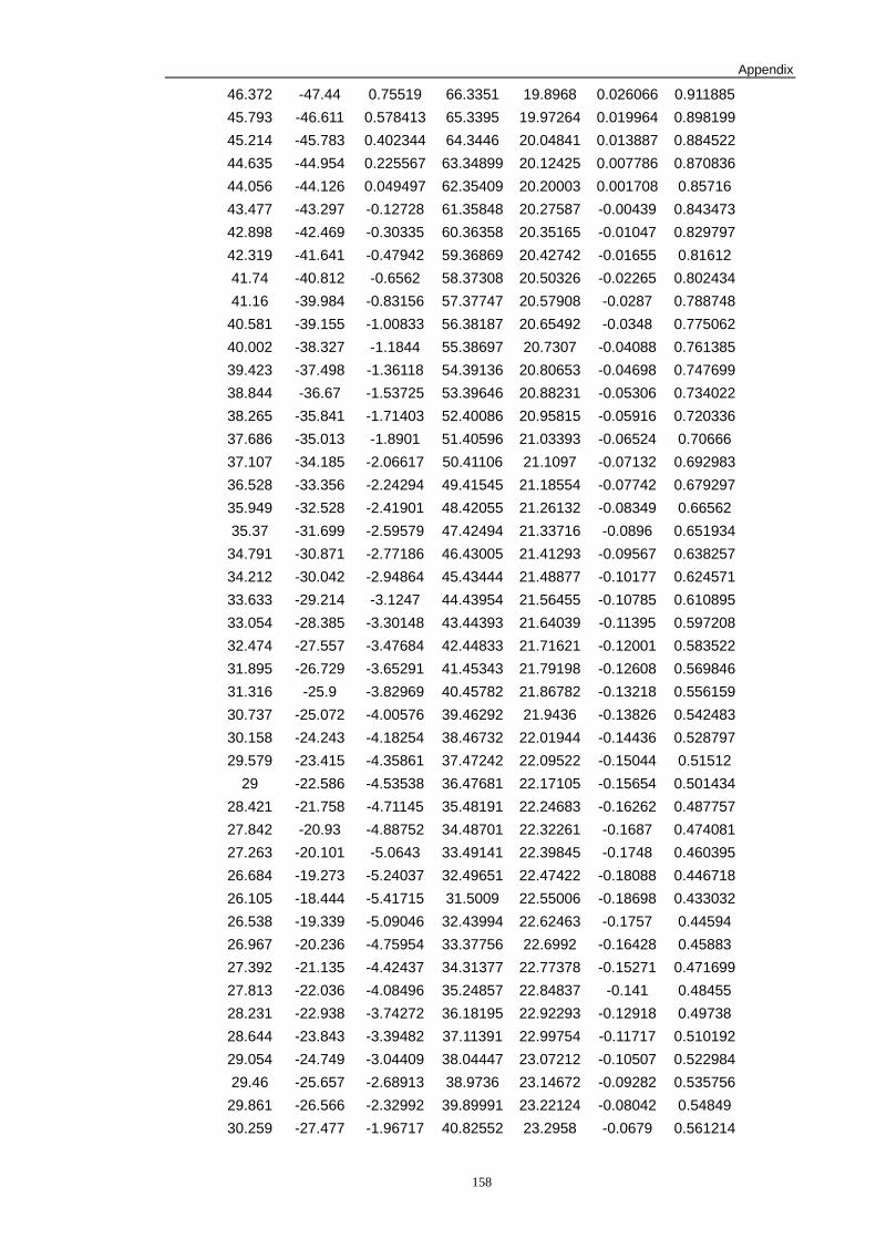
Appendix
158
46.372 -47.44 0.75519 66.3351 19.8968 0.026066 0.91188545.793 -46.611 0.578413 65.3395 19.97264 0.019964 0.89819945.214 -45.783 0.402344 64.3446 20.04841 0.013887 0.88452244.635 -44.954 0.225567 63.34899 20.12425 0.007786 0.87083644.056 -44.126 0.049497 62.35409 20.20003 0.001708 0.8571643.477 -43.297 -0.12728 61.35848 20.27587 -0.00439 0.84347342.898 -42.469 -0.30335 60.36358 20.35165 -0.01047 0.82979742.319 -41.641 -0.47942 59.36869 20.42742 -0.01655 0.8161241.74 -40.812 -0.6562 58.37308 20.50326 -0.02265 0.80243441.16 -39.984 -0.83156 57.37747 20.57908 -0.0287 0.788748
40.581 -39.155 -1.00833 56.38187 20.65492 -0.0348 0.77506240.002 -38.327 -1.1844 55.38697 20.7307 -0.04088 0.76138539.423 -37.498 -1.36118 54.39136 20.80653 -0.04698 0.74769938.844 -36.67 -1.53725 53.39646 20.88231 -0.05306 0.73402238.265 -35.841 -1.71403 52.40086 20.95815 -0.05916 0.72033637.686 -35.013 -1.8901 51.40596 21.03393 -0.06524 0.7066637.107 -34.185 -2.06617 50.41106 21.1097 -0.07132 0.69298336.528 -33.356 -2.24294 49.41545 21.18554 -0.07742 0.67929735.949 -32.528 -2.41901 48.42055 21.26132 -0.08349 0.6656235.37 -31.699 -2.59579 47.42494 21.33716 -0.0896 0.651934
34.791 -30.871 -2.77186 46.43005 21.41293 -0.09567 0.63825734.212 -30.042 -2.94864 45.43444 21.48877 -0.10177 0.62457133.633 -29.214 -3.1247 44.43954 21.56455 -0.10785 0.61089533.054 -28.385 -3.30148 43.44393 21.64039 -0.11395 0.59720832.474 -27.557 -3.47684 42.44833 21.71621 -0.12001 0.58352231.895 -26.729 -3.65291 41.45343 21.79198 -0.12608 0.56984631.316 -25.9 -3.82969 40.45782 21.86782 -0.13218 0.55615930.737 -25.072 -4.00576 39.46292 21.9436 -0.13826 0.54248330.158 -24.243 -4.18254 38.46732 22.01944 -0.14436 0.52879729.579 -23.415 -4.35861 37.47242 22.09522 -0.15044 0.51512
29 -22.586 -4.53538 36.47681 22.17105 -0.15654 0.50143428.421 -21.758 -4.71145 35.48191 22.24683 -0.16262 0.48775727.842 -20.93 -4.88752 34.48701 22.32261 -0.1687 0.47408127.263 -20.101 -5.0643 33.49141 22.39845 -0.1748 0.46039526.684 -19.273 -5.24037 32.49651 22.47422 -0.18088 0.44671826.105 -18.444 -5.41715 31.5009 22.55006 -0.18698 0.43303226.538 -19.339 -5.09046 32.43994 22.62463 -0.1757 0.4459426.967 -20.236 -4.75954 33.37756 22.6992 -0.16428 0.4588327.392 -21.135 -4.42437 34.31377 22.77378 -0.15271 0.47169927.813 -22.036 -4.08496 35.24857 22.84837 -0.141 0.4845528.231 -22.938 -3.74272 36.18195 22.92293 -0.12918 0.4973828.644 -23.843 -3.39482 37.11391 22.99754 -0.11717 0.51019229.054 -24.749 -3.04409 38.04447 23.07212 -0.10507 0.52298429.46 -25.657 -2.68913 38.9736 23.14672 -0.09282 0.535756
29.861 -26.566 -2.32992 39.89991 23.22124 -0.08042 0.5484930.259 -27.477 -1.96717 40.82552 23.2958 -0.0679 0.561214
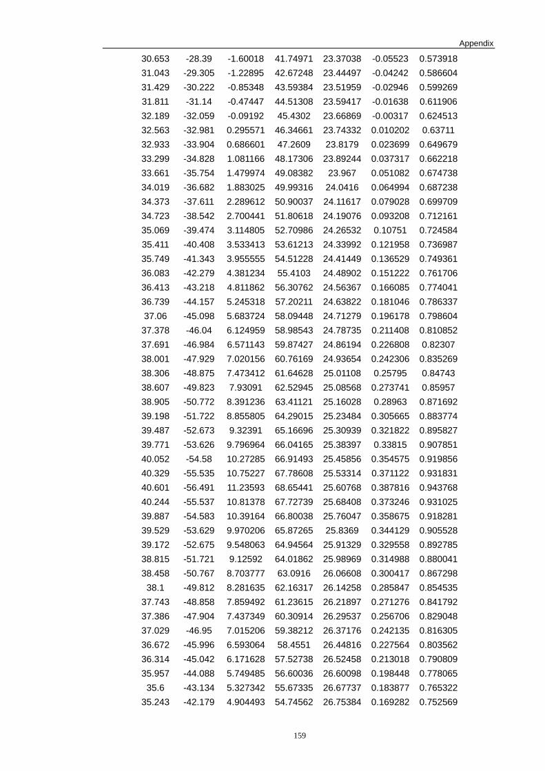
Appendix
159
30.653 -28.39 -1.60018 41.74971 23.37038 -0.05523 0.57391831.043 -29.305 -1.22895 42.67248 23.44497 -0.04242 0.58660431.429 -30.222 -0.85348 43.59384 23.51959 -0.02946 0.59926931.811 -31.14 -0.47447 44.51308 23.59417 -0.01638 0.61190632.189 -32.059 -0.09192 45.4302 23.66869 -0.00317 0.62451332.563 -32.981 0.295571 46.34661 23.74332 0.010202 0.6371132.933 -33.904 0.686601 47.2609 23.8179 0.023699 0.64967933.299 -34.828 1.081166 48.17306 23.89244 0.037317 0.66221833.661 -35.754 1.479974 49.08382 23.967 0.051082 0.67473834.019 -36.682 1.883025 49.99316 24.0416 0.064994 0.68723834.373 -37.611 2.289612 50.90037 24.11617 0.079028 0.69970934.723 -38.542 2.700441 51.80618 24.19076 0.093208 0.71216135.069 -39.474 3.114805 52.70986 24.26532 0.10751 0.72458435.411 -40.408 3.533413 53.61213 24.33992 0.121958 0.73698735.749 -41.343 3.955555 54.51228 24.41449 0.136529 0.74936136.083 -42.279 4.381234 55.4103 24.48902 0.151222 0.76170636.413 -43.218 4.811862 56.30762 24.56367 0.166085 0.77404136.739 -44.157 5.245318 57.20211 24.63822 0.181046 0.78633737.06 -45.098 5.683724 58.09448 24.71279 0.196178 0.798604
37.378 -46.04 6.124959 58.98543 24.78735 0.211408 0.81085237.691 -46.984 6.571143 59.87427 24.86194 0.226808 0.8230738.001 -47.929 7.020156 60.76169 24.93654 0.242306 0.83526938.306 -48.875 7.473412 61.64628 25.01108 0.25795 0.8474338.607 -49.823 7.93091 62.52945 25.08568 0.273741 0.8595738.905 -50.772 8.391236 63.41121 25.16028 0.28963 0.87169239.198 -51.722 8.855805 64.29015 25.23484 0.305665 0.88377439.487 -52.673 9.32391 65.16696 25.30939 0.321822 0.89582739.771 -53.626 9.796964 66.04165 25.38397 0.33815 0.90785140.052 -54.58 10.27285 66.91493 25.45856 0.354575 0.91985640.329 -55.535 10.75227 67.78608 25.53314 0.371122 0.93183140.601 -56.491 11.23593 68.65441 25.60768 0.387816 0.94376840.244 -55.537 10.81378 67.72739 25.68408 0.373246 0.93102539.887 -54.583 10.39164 66.80038 25.76047 0.358675 0.91828139.529 -53.629 9.970206 65.87265 25.8369 0.344129 0.90552839.172 -52.675 9.548063 64.94564 25.91329 0.329558 0.89278538.815 -51.721 9.12592 64.01862 25.98969 0.314988 0.88004138.458 -50.767 8.703777 63.0916 26.06608 0.300417 0.867298
38.1 -49.812 8.281635 62.16317 26.14258 0.285847 0.85453537.743 -48.858 7.859492 61.23615 26.21897 0.271276 0.84179237.386 -47.904 7.437349 60.30914 26.29537 0.256706 0.82904837.029 -46.95 7.015206 59.38212 26.37176 0.242135 0.81630536.672 -45.996 6.593064 58.4551 26.44816 0.227564 0.80356236.314 -45.042 6.171628 57.52738 26.52458 0.213018 0.79080935.957 -44.088 5.749485 56.60036 26.60098 0.198448 0.778065
35.6 -43.134 5.327342 55.67335 26.67737 0.183877 0.76532235.243 -42.179 4.904493 54.74562 26.75384 0.169282 0.752569
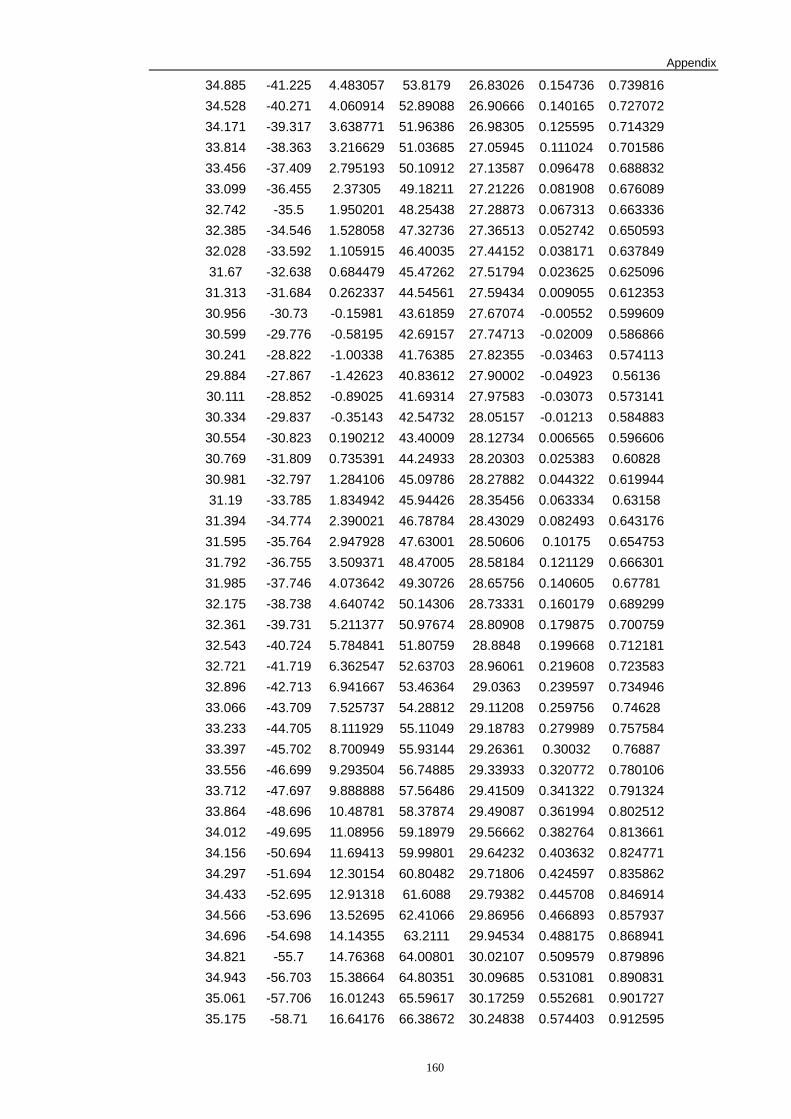
Appendix
160
34.885 -41.225 4.483057 53.8179 26.83026 0.154736 0.73981634.528 -40.271 4.060914 52.89088 26.90666 0.140165 0.72707234.171 -39.317 3.638771 51.96386 26.98305 0.125595 0.71432933.814 -38.363 3.216629 51.03685 27.05945 0.111024 0.70158633.456 -37.409 2.795193 50.10912 27.13587 0.096478 0.68883233.099 -36.455 2.37305 49.18211 27.21226 0.081908 0.67608932.742 -35.5 1.950201 48.25438 27.28873 0.067313 0.66333632.385 -34.546 1.528058 47.32736 27.36513 0.052742 0.65059332.028 -33.592 1.105915 46.40035 27.44152 0.038171 0.63784931.67 -32.638 0.684479 45.47262 27.51794 0.023625 0.625096
31.313 -31.684 0.262337 44.54561 27.59434 0.009055 0.61235330.956 -30.73 -0.15981 43.61859 27.67074 -0.00552 0.59960930.599 -29.776 -0.58195 42.69157 27.74713 -0.02009 0.58686630.241 -28.822 -1.00338 41.76385 27.82355 -0.03463 0.57411329.884 -27.867 -1.42623 40.83612 27.90002 -0.04923 0.5613630.111 -28.852 -0.89025 41.69314 27.97583 -0.03073 0.57314130.334 -29.837 -0.35143 42.54732 28.05157 -0.01213 0.58488330.554 -30.823 0.190212 43.40009 28.12734 0.006565 0.59660630.769 -31.809 0.735391 44.24933 28.20303 0.025383 0.6082830.981 -32.797 1.284106 45.09786 28.27882 0.044322 0.61994431.19 -33.785 1.834942 45.94426 28.35456 0.063334 0.63158
31.394 -34.774 2.390021 46.78784 28.43029 0.082493 0.64317631.595 -35.764 2.947928 47.63001 28.50606 0.10175 0.65475331.792 -36.755 3.509371 48.47005 28.58184 0.121129 0.66630131.985 -37.746 4.073642 49.30726 28.65756 0.140605 0.6778132.175 -38.738 4.640742 50.14306 28.73331 0.160179 0.68929932.361 -39.731 5.211377 50.97674 28.80908 0.179875 0.70075932.543 -40.724 5.784841 51.80759 28.8848 0.199668 0.71218132.721 -41.719 6.362547 52.63703 28.96061 0.219608 0.72358332.896 -42.713 6.941667 53.46364 29.0363 0.239597 0.73494633.066 -43.709 7.525737 54.28812 29.11208 0.259756 0.7462833.233 -44.705 8.111929 55.11049 29.18783 0.279989 0.75758433.397 -45.702 8.700949 55.93144 29.26361 0.30032 0.7688733.556 -46.699 9.293504 56.74885 29.33933 0.320772 0.78010633.712 -47.697 9.888888 57.56486 29.41509 0.341322 0.79132433.864 -48.696 10.48781 58.37874 29.49087 0.361994 0.80251234.012 -49.695 11.08956 59.18979 29.56662 0.382764 0.81366134.156 -50.694 11.69413 59.99801 29.64232 0.403632 0.82477134.297 -51.694 12.30154 60.80482 29.71806 0.424597 0.83586234.433 -52.695 12.91318 61.6088 29.79382 0.445708 0.84691434.566 -53.696 13.52695 62.41066 29.86956 0.466893 0.85793734.696 -54.698 14.14355 63.2111 29.94534 0.488175 0.86894134.821 -55.7 14.76368 64.00801 30.02107 0.509579 0.87989634.943 -56.703 15.38664 64.80351 30.09685 0.531081 0.89083135.061 -57.706 16.01243 65.59617 30.17259 0.552681 0.90172735.175 -58.71 16.64176 66.38672 30.24838 0.574403 0.912595
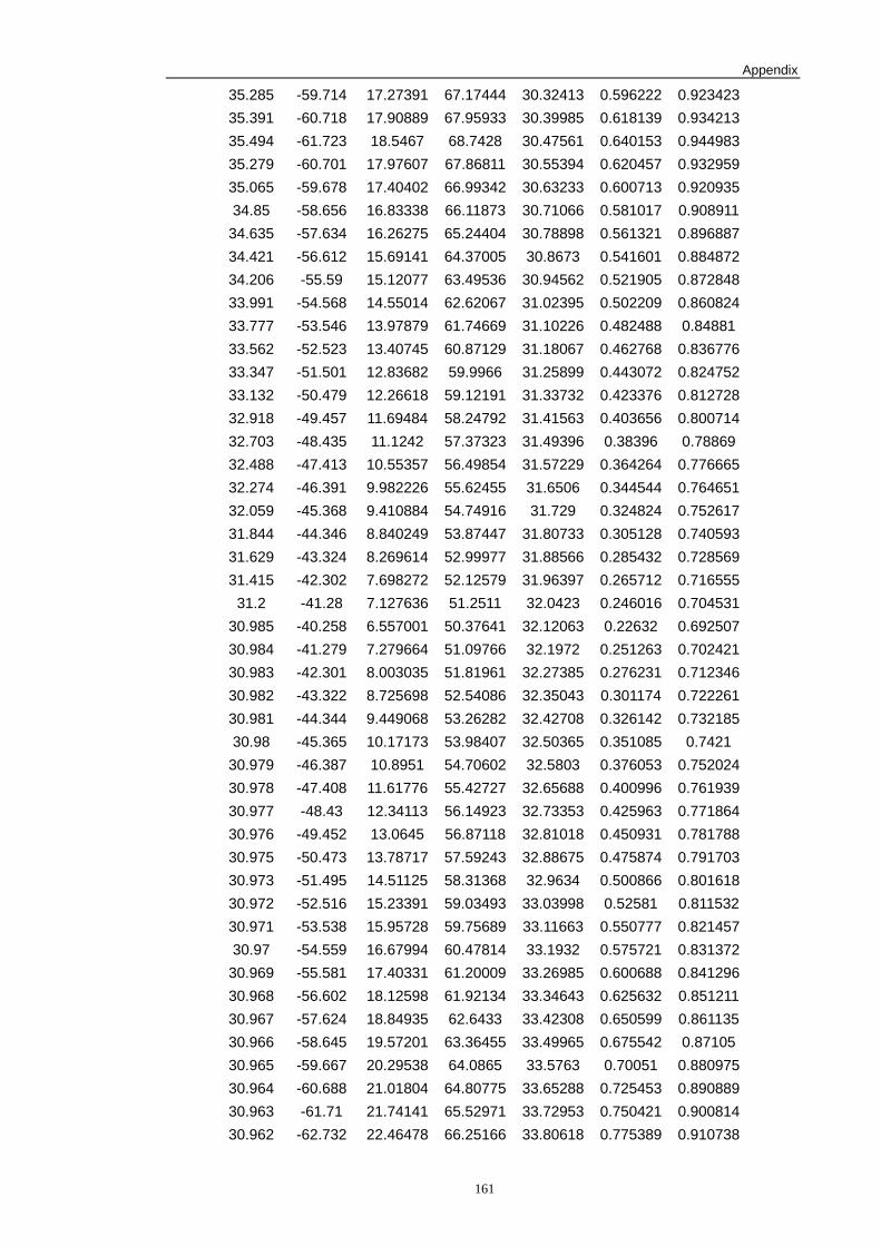
Appendix
161
35.285 -59.714 17.27391 67.17444 30.32413 0.596222 0.92342335.391 -60.718 17.90889 67.95933 30.39985 0.618139 0.93421335.494 -61.723 18.5467 68.7428 30.47561 0.640153 0.94498335.279 -60.701 17.97607 67.86811 30.55394 0.620457 0.93295935.065 -59.678 17.40402 66.99342 30.63233 0.600713 0.92093534.85 -58.656 16.83338 66.11873 30.71066 0.581017 0.908911
34.635 -57.634 16.26275 65.24404 30.78898 0.561321 0.89688734.421 -56.612 15.69141 64.37005 30.8673 0.541601 0.88487234.206 -55.59 15.12077 63.49536 30.94562 0.521905 0.87284833.991 -54.568 14.55014 62.62067 31.02395 0.502209 0.86082433.777 -53.546 13.97879 61.74669 31.10226 0.482488 0.8488133.562 -52.523 13.40745 60.87129 31.18067 0.462768 0.83677633.347 -51.501 12.83682 59.9966 31.25899 0.443072 0.82475233.132 -50.479 12.26618 59.12191 31.33732 0.423376 0.81272832.918 -49.457 11.69484 58.24792 31.41563 0.403656 0.80071432.703 -48.435 11.1242 57.37323 31.49396 0.38396 0.7886932.488 -47.413 10.55357 56.49854 31.57229 0.364264 0.77666532.274 -46.391 9.982226 55.62455 31.6506 0.344544 0.76465132.059 -45.368 9.410884 54.74916 31.729 0.324824 0.75261731.844 -44.346 8.840249 53.87447 31.80733 0.305128 0.74059331.629 -43.324 8.269614 52.99977 31.88566 0.285432 0.72856931.415 -42.302 7.698272 52.12579 31.96397 0.265712 0.716555
31.2 -41.28 7.127636 51.2511 32.0423 0.246016 0.70453130.985 -40.258 6.557001 50.37641 32.12063 0.22632 0.69250730.984 -41.279 7.279664 51.09766 32.1972 0.251263 0.70242130.983 -42.301 8.003035 51.81961 32.27385 0.276231 0.71234630.982 -43.322 8.725698 52.54086 32.35043 0.301174 0.72226130.981 -44.344 9.449068 53.26282 32.42708 0.326142 0.73218530.98 -45.365 10.17173 53.98407 32.50365 0.351085 0.7421
30.979 -46.387 10.8951 54.70602 32.5803 0.376053 0.75202430.978 -47.408 11.61776 55.42727 32.65688 0.400996 0.76193930.977 -48.43 12.34113 56.14923 32.73353 0.425963 0.77186430.976 -49.452 13.0645 56.87118 32.81018 0.450931 0.78178830.975 -50.473 13.78717 57.59243 32.88675 0.475874 0.79170330.973 -51.495 14.51125 58.31368 32.9634 0.500866 0.80161830.972 -52.516 15.23391 59.03493 33.03998 0.52581 0.81153230.971 -53.538 15.95728 59.75689 33.11663 0.550777 0.82145730.97 -54.559 16.67994 60.47814 33.1932 0.575721 0.831372
30.969 -55.581 17.40331 61.20009 33.26985 0.600688 0.84129630.968 -56.602 18.12598 61.92134 33.34643 0.625632 0.85121130.967 -57.624 18.84935 62.6433 33.42308 0.650599 0.86113530.966 -58.645 19.57201 63.36455 33.49965 0.675542 0.8710530.965 -59.667 20.29538 64.0865 33.5763 0.70051 0.88097530.964 -60.688 21.01804 64.80775 33.65288 0.725453 0.89088930.963 -61.71 21.74141 65.52971 33.72953 0.750421 0.90081430.962 -62.732 22.46478 66.25166 33.80618 0.775389 0.910738

Appendix
162
30.961 -63.753 23.18745 66.97291 33.88275 0.800332 0.92065330.959 -64.775 23.91152 67.69416 33.9594 0.825324 0.93056830.958 -65.796 24.63419 68.41541 34.03598 0.850267 0.94048330.957 -66.818 25.35756 69.13737 34.11263 0.875235 0.95040730.956 -67.839 26.08022 69.85861 34.1892 0.900178 0.96032230.955 -68.861 26.80359 70.58057 34.26585 0.925146 0.97024630.954 -69.882 27.52625 71.30182 34.34243 0.950089 0.98016130.953 -70.904 28.24962 72.02378 34.41908 0.975057 0.99008530.952 -71.925 28.97229 72.74502 34.49565 1 1
* Run 3 & 4 (Feed rate = 900 mm/min)
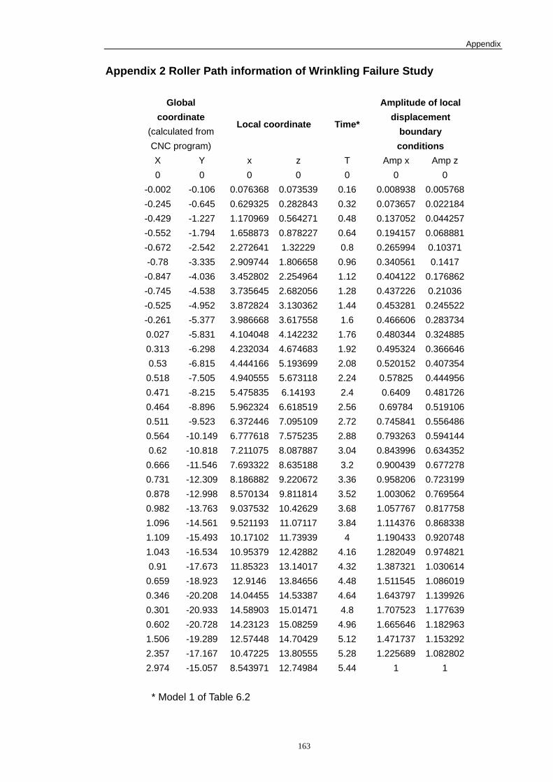
Appendix
163
Appendix 2 Roller Path information of Wrinkling Failure Study
Global coordinate
(calculated from CNC program)
Local coordinate Time*
Amplitude of local displacement
boundary conditions
X Y x z T Amp x Amp z 0 0 0 0 0 0 0
-0.002 -0.106 0.076368 0.073539 0.16 0.008938 0.005768-0.245 -0.645 0.629325 0.282843 0.32 0.073657 0.022184-0.429 -1.227 1.170969 0.564271 0.48 0.137052 0.044257-0.552 -1.794 1.658873 0.878227 0.64 0.194157 0.068881-0.672 -2.542 2.272641 1.32229 0.8 0.265994 0.10371-0.78 -3.335 2.909744 1.806658 0.96 0.340561 0.1417 -0.847 -4.036 3.452802 2.254964 1.12 0.404122 0.176862-0.745 -4.538 3.735645 2.682056 1.28 0.437226 0.21036-0.525 -4.952 3.872824 3.130362 1.44 0.453281 0.245522-0.261 -5.377 3.986668 3.617558 1.6 0.466606 0.2837340.027 -5.831 4.104048 4.142232 1.76 0.480344 0.3248850.313 -6.298 4.232034 4.674683 1.92 0.495324 0.3666460.53 -6.815 4.444166 5.193699 2.08 0.520152 0.4073540.518 -7.505 4.940555 5.673118 2.24 0.57825 0.4449560.471 -8.215 5.475835 6.14193 2.4 0.6409 0.4817260.464 -8.896 5.962324 6.618519 2.56 0.69784 0.5191060.511 -9.523 6.372446 7.095109 2.72 0.745841 0.5564860.564 -10.149 6.777618 7.575235 2.88 0.793263 0.5941440.62 -10.818 7.211075 8.087887 3.04 0.843996 0.6343520.666 -11.546 7.693322 8.635188 3.2 0.900439 0.6772780.731 -12.309 8.186882 9.220672 3.36 0.958206 0.7231990.878 -12.998 8.570134 9.811814 3.52 1.003062 0.7695640.982 -13.763 9.037532 10.42629 3.68 1.057767 0.8177581.096 -14.561 9.521193 11.07117 3.84 1.114376 0.8683381.109 -15.493 10.17102 11.73939 4 1.190433 0.9207481.043 -16.534 10.95379 12.42882 4.16 1.282049 0.9748210.91 -17.673 11.85323 13.14017 4.32 1.387321 1.0306140.659 -18.923 12.9146 13.84656 4.48 1.511545 1.0860190.346 -20.208 14.04455 14.53387 4.64 1.643797 1.1399260.301 -20.933 14.58903 15.01471 4.8 1.707523 1.1776390.602 -20.728 14.23123 15.08259 4.96 1.665646 1.1829631.506 -19.289 12.57448 14.70429 5.12 1.471737 1.1532922.357 -17.167 10.47225 13.80555 5.28 1.225689 1.0828022.974 -15.057 8.543971 12.74984 5.44 1 1
* Model 1 of Table 6.2


![Investigation of Tissue Engineering Scaffolds for ...doktori.bibl.u-szeged.hu/4158/1/phd_thesis_ zsedenyi.pdf · tissue engineering, especially for the fabrication of scaffolds [14]](https://img.pdfslide.us/doc/110x75/5f9136fac4be4300fb3b3c1b/investigation-of-tissue-engineering-scaffolds-for-zsedenyipdf-tissue-engineering.jpg)