Embed Size (px)
Citation preview

Documents de travail du Laboratoire d’Economie et de Gestion
Working Papers
NEIGHBORHOOD EFFECTS IN SPATIAL HOUSING VALUE MODELS THE CASE OF THE METROPOLITAN AREA OF PARIS (1999).
Catherine Baumont, Diégo Legros
Université de Bourgogne & CNRS UMR 5118 Laboratoire d’Economie et de Gestion
Pôle d’Economie et de Gestion, 2 boulevard Gabriel, 21000 Dijon, France
e2009-09 Equipe Analyse et Modélisation des Interactions Economiques (AMIE)
Laboratoire d’Economie et de Gestion
Université de Bourgogne & CNRS UMR 5118 Pôle d’Economie et de Gestion - 2 boulevard Gabriel BP 26611 - F21066 DIJON cedex Tel. +33 (0)3 80 39 54 30 Fax +33 (0)3 80 39 54 43 [email protected] - www.u-bourgogne.fr/leg
NEIGHBORHOOD EFFECTS IN SPATIAL HOUSING VALUE MODELS THE CASE OF THE METROPOLITAN AREA OF PARIS (1999)
Catherine Baumont(1) & Diégo Legros(2) Laboratoire d’Economie et de Gestion (UMR 5118 CNRS), Université de Bourgogne, France
Mai 2009
Abstract : In hedonic housing models, the spatial dimension of housing values are traditionally processed by the impact of neighborhood variables and accessibility variables. In this paper we show that spatial effects might remain once neighborhood effects and accessibility have been controlled for. We notably stress on three sides of neighborhood effects: social capital, social status and social externalities and consider the accessibility to the primary economic center as describing the urban spatial trend. Using spatial econometrics specifications of the hedonic equation, we estimate whether spatial effects impact the housing values. Our empirical case concerns the Metropolitan Area (MA) of Paris in France which is divided in 2 636 neighborhood areas. We estimate the housing price distribution from a sample of 21,000 apartments sold in 1999. Our empirical results highlight the lumpy distribution of unit price along the general decreasing spatial trend from the Central Business District once neighborhood effects have been introduced. More precisely, a spatial error model is estimated revealing a positive and significance spatial effects across housing values which extend beyond their neighborhood area. Social capital, social status and social externalities play local role and may positively or negatively impact the housing prices. We showed a positive impact of diversified building patterns but a negative impact of social mixity which is somewhat conflictual but which is in fact in line with many current questions about social segregation and spatial segregation in urban areas.
Keywords : Hedonic model, housing value, neighborhood effects, spatial econometrics
Résumé : On considère généralement, dans les modèles hédoniques de valeurs immobilières, que l’influence de la localisation
sur la formation des prix est suffisamment appréhendée par des variables explicatives d’attributs des voisinages et
d’accessibilité. Dans cet article, nous montrons que des effets spatiaux non captés subsistent malgré l’introduction de ces
variables de voisinage et d’accessibilité. Plus précisément nous distinguons trois sortes d’effets de voisinage : ceux liés soit au
capital social ou au statut social des quartiers et ceux liés aux externalités sociales. Le trend spatial est quant à lui apprécié par
la distance au Central Business District comme préconisé par les modèles d’économie urbaine. L’estimation de l’existence des
effets spatiaux et de leurs impacts sur les valeurs immobilières est faite par l’estimation de modèle hédonique spatiaux. Notre
étude empirique porte sur l’aire métropolitaine de Paris en France qui est composée de la ville de Paris et de la Petite
Couronne et compte 2 636 aires de voisinage. Nous estimons une fonction hédonique des valeurs immobilières à partir d’un
échantillon de 21 000 ventes d’appartement en 1999. La présence d’erreurs spatialement autocorrélées indique que des effets
spatiaux persistent au-delà du trend spatial et ceci quels que soient les effets de voisinage considérés. L’estimation du modèle
SEM révèle des effets spatiaux positifs et significatifs des valeurs immobilières dans l’aire métropolitaine de Paris. Les effets de
voisinages sont également significatifs et jouent positivement ou négativement sur les prix des appartements. Nous montrons
par exemple l’impact positif de la diversification des types d’habitats selon leur ancienneté tandis que l’impact d’une
diversification sociale est négatif : ce résultats apparaît ainsi contradictoire mais en cohérence avec les conclusions mitigées
des réflexions sur la mixité sociale.
Mots clés : Modèle hédonique, valeur immobilière, effets de voisinage, économétrie spatiale
JEL Classification : C120, C520, R140, R210
(1) [email protected], Université de Bourgogne, Laboratoire d’Economie et de Gestion, Pôle d'Economie et de Gestion, B.P. 26611, 21066 Dijon Cedex, France, tél : 03.80.39.35.21 Fax : 03.80.39.54.43
(2) [email protected], Laboratoire d’Economie et de Gestion, Université de Bourgogne, Pôle d'Economie et de Gestion, B.P. 26611, 21066 Dijon Cedex, tél : 03.80.39.35.20, Fax : 03.80.39.54.43
This paper has been presented at the 49 congrès de la sSociété Canadienne de Sciences Economiques, Saint-Adèle, 26èmes
Journées de Microéconomie Appliquée, Dijon, 4-5 juin 2009.
NEIGHBORHOOD EFFECTS IN SPATIAL HOUSING VALUE MODELS
THE CASE OF THE METROPOLITAN AREA OF PARIS (1999)
Catherine Baumont & Diégo Legros
Laboratoire d’Economie et de Gestion (CNRS), Université de Bourgogne, France
1. Introduction
Hedonic housing price equations are mainly estimated to produce relevant evaluation of the housing price
distribution and of the implicit prices of housing attributes. These estimations are major inputs in the investigation of
housing market by the analysis of consumer demand for attributes. As indicated by the abundant literature on hedonic
housing price models, such studies find numerous applications in business, economic and social fields linked to real
estate investment decisions, mortgage markets, housing policies and programs, local tax policies, urban environmental
planning and urban development.
Empirical specifications show that housing values may be explained by a large set of attributes generally grouped
into three subsets: 1/ structural or internal variables describing the physical characteristics of housing, 2/ neighborhood or
environmental variables depicting the quality of amenities and the economic and social characteristics of the
neighborhood, and 3/ accessibility or spatial variables including distances to major places of employment, to major
amenities (leisure, shopping and public facilities, outstanding sites, etc.), and to road infrastructures and transport access
points (train stations, subway stations, major streets, highways, airports, etc.). Such a large specification implies that the
housing choice insures the best combination of a large set of attributes sought by the household: internal characteristics
of house or apartment, external characteristics of neighborhood and spatial characteristics of the location. More precisely,
it implies that the housing choice doesn’t reduce to the choice of an house or an apartment but it includes a neighborhood
choice and a location choice too. It is then supported both by the new consumer theory (Lancaster, 1966) applied to real
estate properties and to neighborhoods and by the urban economic theory (Alonso, 1964, Muth, 1969, Fujita, [28]) applied
to household choices.
Since housing, neighborhood and location choices go hand with hand, some main questions arise about the
dependence forms at work. Why housing and neighborhood choices are dependent ? Does it produce dependence within
the spatial distribution of housing values ? What kinds of estimation problems does it implies ?
Our paper is a contribution to these questions and focus on neighborhood effects and on spatial effects. On one
hand, the concept of neighborhood effects explains interdependencies between a neighborhood and its residents and is
strongly based on the economic and social status of the districts within an urban area. Studying the impact of
neighborhood effects on housing values fall within the scope of urban policies. In fact, urban policy makers are often
confronted with problems of urban segregation and exclusion, obsolescence of older areas, and social marginality in
inner-city areas, challenging them to find appropriate levers for urban regeneration policies (Adair et al. [2]). On the other
hand, the concept of spatial effects refers to spatial dependence and involves both technical and empirical issues in the
estimation of the hedonic model. Housing price distributions are strongly affected by spatial effects, mainly because of
neighborhood effects, and then appropriate econometric tools are used to model housing prices and to estimate the
hedonic equation.
Our case study is the Metropolitan Area of Paris in France which is bounded in this paper by the first ring around
the city of Paris. The MA spreads on a total surface area of 762 km² for a population of 6.2 millions inhabitants and 2.8
millions of apartments. We estimate the housing price distribution from a sample of 21,000 apartment transactions in
1999. Neighborhood effects are defined at the IRIS scale which is the finest geographical statistical unit at the city level for
which French data are provided. The MA of Paris is divided in 2 636 IRIS.
The paper is organized as follows. In the next part, we set out the conceptual framework. We present the core
concepts of spatial dependence and neighborhood effects we deal with in housing values estimations. The third section
presents our empirical framework and the empirical findings. We present the study area, the data and the variables.
Spatial effects are detected and a Spatial Error Model specification is then estimated revealing a positive spatial effect on
housing prices. We first estimate a core model including housing attributes and accessibility variables which we
successively extend to other sets of variables depicting the economic and social dimensions of the neighborhood effects.
The paper concludes with a summary of key findings.
2. Spatial effects, neighborhood effects and housing values in urban areas
Since the concern here is with neighborhood effects and spatial effects, it is necessary to define these concepts
and to outline the associated empirical issues.
2.1 Controlling for spatial effects in housing prices
Spatial effects mean that the observations of a phenomena are interdependent and refer to spatial autocorrelation
and spatial heterogeneity. “Spatial” denotes that patterns of interdependencies are geographically based but by extend,
“spatial effects” may be used for all kinds of interdependencies across observations based on social, institutional, cultural,
economic… types of “proximity”.
2.1.1 Spatial autocorrelation and spatial heterogeneity
Spatial autocorrelation can be defined as the coincidence of value similarity with location similarity (Anselin, [5]).
This idea is in line with the Tobler's Law of Geography (Tobler, [50]), which states that observations closer together in
space are more likely to have similar characteristics than those that are further apart. Therefore, there is positive spatial
autocorrelation when similar values of a random variable measured on various locations tend to cluster in space while
negative spatial autocorrelation means that similar values tend to be dispersed. Applied to housing values, its means that
high unit prices tend to be more geographically clustered (as well as low unit prices) than it could be randomly observed in
urban areas.
Spatial heterogeneity means in turn that economic behaviors are not stable over space. These variations follow for
example specific geographical patterns such as East and West, or North and South... or may be observed more locally
from one district to another. Such a spatial heterogeneity characterizes the distribution of housing unit prices in urban
areas where historical development periods and/or urban development policies supported particular population residential
patterns. This question is obviously a central issue for urban planners and has introduced a new policy thinking as urban
renewal cycles have been evidenced.
In addition, the links between spatial autocorrelation and spatial heterogeneity are quite complex since spatial
heterogeneity often occurs jointly with spatial autocorrelation in applied econometric studies (Anselin, [5]). Moreover,
spatial autocorrelation and spatial heterogeneity may be observationally equivalent: in polarization phenomena, a spatial
cluster of extreme residuals in the center may be interpreted as heterogeneity between the center and the periphery or as
spatial autocorrelation implied by a spatial stochastic process yielding clustered values in the center.
From a technical perspective, spatial effects, are known to engender estimation since statistical inference based on
OLS is not reliable when heterogeneity or spatial dependence is present (Anselin, [4], [5]) Empirically, three kinds of
issues arise from spatial effects First, since spatial effects represent spatial interdependencies across observations, the
interaction pattern has to be defined by a spatial weight matrix. Second, it is necessary to test whereas spatial
autocorrelation and/or spatial heterogeneity characterize the housing price distribution given to the geographical pattern
describing them. For example, if spatial autocorrelation and spatial heterogeneity occur jointly then we can identify spatial
clusters of similar housing values whereas the type of spatial association differs between clusters: clusters of high values

against clusters of low values for instance. Finally, when spatial effects are confirmed, it is therefore necessary to estimate
the spatial hedonic equation with appropriate econometric methods.
2.1.2. Spatial effects in housing prices
More precisely, spatial dependences characterize housing values and hedonic models for several reasons
explained by economic and social factors.
Following urban economic theories, the spatial organization of households and firms in urban areas results from
economic balances involving preferences, commuting or transportation costs, land or housing expenses and spatial
externalities (Fujita and Thisse, [29]). Spatial densities of population or firms and spatial distributions of land values,
housing values or office values are then produced stressing on the role played by economic centers, which concentrate
the urban economic activities, in this spatial organization (Baumont et al., [10]). Considering for example residential
patterns and the New Urban Economics tradition derived from the Alonso-Muth model (Alonso, [3]; Muth, 1969), the unit
price of housing should fall with distance to the primary and predominant economic center named Central Business
District (CBD). As a result, real estate properties clustering at a similar distance to CBD tend to have similar values and
are spatially autocorrelated. Despite changes in the spatial organization of metropolitan areas, this spatial scheme acts as
a spatial trend and remains true for ages (McMillen, [41]). However, the NUE core model has been extended to take
account of local irregularities created by the development of a polycentric pattern: the housing price distribution exhibits
an overall peak at the CBD location and local peaks at the location of subcenters (Papageorgiou and Mullaly, [45]), as has
been empirically well documented (Baumont and Le Gallo, [12]). Other forms of empirical functional specifications have
been developed to better capture the irregularities of the housing price distribution through cubic spline specification, for
example. In these approaches, accessibility variables to secondary economic centers are included in the hedonic
equation and can take various distance based forms. Local irregularities have also been handled by the use of
explanatory variables indicating the existence of housing sub-markets (Basu and Thibodeau, [8]; Wilhelmsson, [52]), or
spatial regimes (Páez et al., [44]).
Turning to structural and neighborhood attributes helps to focus on other sources of spatial dependences which
rely on a complex combination of two principles. One is the fact that housing is a durable good located in a durable
environment: houses and buildings within a neighborhood were often built at the same time and tend to have similar
structural characteristics. Real estate properties within the same neighborhood capitalize shared positive or negative
amenities, have similar access to labor markets and public facilities… Then in the same neighborhood, housing prices
tend to be similar and they can differ across different neighborhoods, which results in spatial autocorrelation and spatial
heterogeneity. The other principle states that social and economic attributes of neighborhoods and of their residents are
closely correlated. The poor can’t bid for high level of housing services and live in disadvantaged districts characterized by
low social and economic status whereas the rich bid for high level of residential service and live in good neighborhoods.
Hence, modeling housing demand and neighborhood location choice as a joint process appears more relevant than
considering them as independent choices (Ioannides and Zabel, [35]). Accordingly housing prices in the same
neighborhood or in a cluster of neighborhoods may be spatially correlated.
In addition, the residuals produced by hedonic models of housing prices may be spatially correlated owing to
measurement errors on the variables, omitted variables, or other forms of hedonic model misspecifications (McMillen,
[40]). In fact, many neighborhood and accessibility variables taking part in the housing value equations are difficult to
measure because they are unobservable (like the quality of public facilities), or complex (the crime rate or prevalence of
violence, the social and economic composition of a district), or because they depend on the prior identification of major
areas and places (CBD and major employment subcenters, major recreational places, major outstanding sites, etc.) and
the way accessibility to them can be measured. In addition, such variables are rarely available in data bases. Even if
relevant and reliable data are available, the problem of identifying the relevant neighborhood boundaries may remain
(Dubin, [22]; Basu and Thibodeau, [8]). Finally, selecting the best set of explanatory variables and the correct model
specification is difficult (Sheppard, [48]).
In this paper we mainly focus on the spatial autocorrelation issue1 and stress on the neighborhood attributes
whose effects on housing values and urban patterns have been documented in recent literature on neighborhood effects.
2.2. Neighborhood effects and housing values
The concept of neighborhood effect is quite complex and receives various definition according to the theoretical
field in use. Urban renewal preoccupations offer some interesting evidence in line with the impact of neighborhood effects
on housing values in urban areas.
2.2.1. Neighborhood effects: some definitions
From a sociological point of view, the concept of neighborhood effect (Wilson, [53]) underlines the dependence
effects between the social and economic attributes of districts and those of their residents. Stigma attached to poor urban
1 Taking care of a large set of neighborhood variables gives a first approach of the heterogeneity issue in the paper but this problem is far from being considered here but will be part of our research agenda.

districts and urban regeneration policies as levers to improve the quality of life in neighborhoods and to attract new
residents... are good illustrations of the cumulative and lasting processes involved by neighborhood effects especially on
individual behaviors, peer group influence, social disparities, spatial segregation and poverty traps.
The economic nature of neighborhood effects refers to externalities and interactions (Durlauf, [25], Manski, [39]).
Within a neighborhood, social, economic and institutional attributes may be the source of external increasing returns or
spillovers intensified by social proximities as well as many types of imitative or conditional behaviors may occur and grow
under the influence of social interactions.
The geographical nature of neighborhood is directly derived from its mathematical definition and refers to spatial
proximities which has been empirically interpreted as a small area. Then neighborhood designs a small sector of a large
urban area generally bounded by streets, composed of one block or a set of contiguous blocks and if residential
essentially occupied by housings.
In hedonic model of housing values, neighborhood variables refer to this geographical meaning and allow to
describe the attributes of the small area where the housing is located. The attributes of buildings, the presence of
amenities, eventually supplemented by a set of social and economic status of the neighborhoods are traditionally
considered. Still considering the economic and sociological natures of neighborhood effects in hedonic housing value
models is not directly addressed but is documented in some theoretical and empirical papers.
2.2.2 Neighborhood effects, urban patterns and housing values: some evidence
Economic theory of urban decline and renewal (Brueckner, [15]; Brueckner and Rosenthal, [16], Rosenthal, [47];
Yacovissi and Kern, [54]) gives an interesting starting point to understand how residential urban patterns change over
times. Given the New Urban Economic tradition, residential densities and housing unit prices decline with the distance to
the primary economic center (Central Business District: CBD). According to their preferences, the spatial distribution of
households by income levels is in favor of declining (respectively increasing) incomes with the distance to the CBD in the
European cities (resp. American cities). In fact, neighborhood characteristics or local amenities (Brueckner et al. [17]),
including natural heritage, heritage sites, architectural characteristics of buildings, have a big effect on the residential
location of rich and poor in metropolitan areas, specially the inner-city location of lower-income households in US cities,
and the inner-city location of upper-income households in European cities. Cultural amenities act as a local force
enhancing concentration in city centres (Baumont and Guillain [11]). On the contrary, residential urban cycles models
show that History, urban development and urban policies may affect this general trends when, as housing get older, rich
households leave them and move to other districts with modern housing sometimes built in formerly deprived districts but
currently renew through urban development policies.

The impacts of social and economic attributes of neighborhoods on housing values has been recently well
documented by the literature on neighborhood effects and urban renewal policies (Baumont, [9]). Economic theory of
urban decline and renewal has collected interesting empirical evidence for US cities (Aaronson, [1]; Brueckner and
Rosenthal, [16]; Rosenthal, [47]; Dye and McMillen, [26]) showing that the age of housing explained neighborhood
dynamics in terms of decline and renewal cycles, alongside local amenities (Brueckner and al, [17]) and traditional
residential choice factors (transportation costs and housing demand). Since housing is a normal good, richer households
are attracted by new buildings, i.e. high levels of housing services, whereas poor households locate in older buildings with
lower levels of housing services. Extrapolating and considering a city neighborhood, if it is assumed that housing services
deteriorate with the age of buildings, poor households will occupy old buildings vacated by rich households and when old
buildings are demolished and replaced by new ones then rich households will come back. Considering a less segregated
process, improving housing services in a poor neighborhood may raise its standing dissuading higher income population
from moving out and attracting higher-income new residents as well (Cummings and DiPasquale, [19]).
These approaches indeed raise an interesting question about the nature of spatial externalities in connection with
social and economic attributes of a neighborhood. Empirical studies, mainly addressed to US cities, give some interesting
but somewhat mitigated results. For example, it is straightforward that specialization may produce positive externalities in
terms of social network benefits while “mixity” may produce positive effects in terms of social capital benefits. Studying
housing values in Baltimore, Dubin and Sung [24] showed that the socio-economic status and racial composition of the
neighborhood affect housing prices more than the quality of public services. Racial segregation behaviors studied in some
US cities (Cutler et al. [21]) may influence housing prices depending on a community’s willingness to pay to keep its
identity. Studying the influence of neighborhood externalities on the neighborhood’s economic status on a panel of
metropolitan areas in the US, Rosenthal [47] reports a negative influence for race and for the population aged 15–29 but a
positive influence for the presence of homeowners and of individuals with college degrees. Using data on metropolitan
areas from the American Housing Survey, Ioannides [34] shows that housing maintenance decisions rely on spatial
interactions between homeowners within small residential neighborhood. The influence of income mixing remains
mitigated depending on the level of the average income in the neighborhood: a positive impact is shown for middle-
income communities but a negative one for the lowest and highest income categories. Social status and social capital of
the neighborhood are strong determinants of neighborhood dynamics too through snowball effects: as the average
income level falls, rich households move away; as the proportion of highly educated individuals increases in the
neighborhood, more rich households move into the neighborhood.
Concerning building project policies, their impacts on property values have received little attention in the empirical
literature although negative or positive effects could be expected depending on whether the building projects succeed or
fail in creating positive amenities and externalities. In fact, different effects are generally expected, which could result in
diametrically opposed amenities or externalities. Concerning public housing projects falling in urban renewal policies, they
may have direct positive impacts on neighboring properties as noted above. Against this, public housing projects allegedly
increase congestion and noise, attract a majority of low-income families, thereby reinforcing the ill repute of the districts,
and drive down housing values. Rabiega et al. [46] showed a positive overall effect in the case of Portland, Oregon. By
contrast Johnson and Ragas [36], studying land values in the New Orleans CBD, explicitly introduced distance to a large
housing project and expected a negative influence since such projects are widely perceived as sources of crime.
However, they failed to prove this assumption owing to the lack of transactions in these areas and their surroundings.
Rosenthal [47], reviewing a panel of US metropolitan areas, shows that the presence of public housing has no significant
effect on the neighborhood’s economic status but that the Low-Income Housing Tax Credit Program has a positive impact
on the neighborhood’s economic status in lower-income neighborhoods. Other ambiguous results are reported for US
housing policies devised to increase quality of life and economic status in neighborhoods by promoting home ownership in
redevelopment areas. In Philadelphia, where two housing developments were implemented in distressed neighborhoods,
new homeowners do not really improve their quality of life. Nor is any evidence found of local benefits for adjacent real-
estate prices and economic activities (Cumming et al., [20]). By contrast, an housing development in New York City does
seem to have produced positive benefits on home prices in nearby areas (Ellen et al., [27]).
Three main conclusions can be drawn from these empirical studies. First, neighborhood effects have strong
impacts on housing values. Second, neighborhood effects refer to complex mechanisms but may be approximated by a
relatively small set of attributes: economic and social characteristics of population and housing policies. Third, taking care
of neighborhood effects in hedonic models highlights local impacts along the general spatial pattern of decreasing housing
unit prices from distance to the CBD.
Our paper is a contribution to these topics at three levels. First, we estimate an hedonic equation which takes care
of social and economic dimension of the neighborhood effect. Second, we extend the model to take care of spatial
dependence and spatial trend. Finally we study a French city: the Metroplitan Areas of Paris.
More precisely, following Rosenthal [47], we assume that neighborhood effects involve economic, social and
housing policies issues. More precisely, we define an economic effect and a social effect which will be introduced in the
hedonic model to estimate. The economic neighborhood effect depends on the economic status defined by the population
income and on urban renewal policies since richer households are attracted by new buildings. The social neighborhood
effect rests on social capital, social status and social externalities. The social capital mainly relies on three types of
households: the presence of educated individuals, the presence of homeowner and the presence of prime ages workers.
The racial composition of the population and public housing projects define the social status. Finally social externalities
rely on the urban density.

Turning to the spatial trend, since accessibility to the Central Business District keeps on act upon housing unit
prices, even in large Metropolitan Areas (McMillen [41]), we consider a spatial trend defines by the distance of the real
estate property to the core of the Metropolitan
Finally, despite the fact that hedonic housing price models include accessibility or neighborhood variables, which
tend to introduce spatial effects into the modelling and estimating processes, only a few empirical studies have applied
appropriate econometric techniques to detect and take into account such spatial effects. Taking care of spatial effects
means that even when neighborhood and accessibility variables are included as explanatory variables in housing value
functions, spatial dependency might remain. It is shown that using spatial econometric techniques is better than ignoring
the dependencies in the data (Dubin, [23], Pace and Gilley, [43], Pace et al., [42]). Moreover, taking into account spatial
autocorrelation improves the estimates and the forecasts on real estate markets (see for example Anselin and Le Gallo,
[7]; Basu and Thibodeau, [8]; Baumont, [9]; Beron and al., [13]; Can and Megboluge, [18]; Dubin, [23]; Gilley and al., [30];
LeSage and Pace, [38]; Pace and Gilley, [42]; Páez et al., [44]; Tse, [51]; Wilhelmsson, [52]).
3. Empirical framework and econometric results
In this part, we first describe our empirical strategy used to estimate the impact of spatial effects and neighborhood
variables on housing values in the Metropolitan Area of Paris. The empirical findings are presented in the second part.
3.1. The empirical strategy
We first describe the Metropolitan Area of Paris, the data and variables used in our empirical studies. Estimating
an hedonic housing value equation with spatial effect needs some tools described in the second part.
3.1.1 The Metropolitan Area of Paris
Our case study is the Metropolitan Area of Paris in France which is bounded in this paper by the first ring around
the city of Paris. The first ring covers three départements: Hauts de Seine, Seine Saint Denis et Val de Marne (Map 1).
The MA spreads on a surface area of 762.4 km² for a population of 6.2 million inhabitants2. The MA has 3.15 million
housings including 2.8 million apartments. This is the most urbanized metropolitan area in France with an average
population density reaching 26,000 hab/km2 in the city of Paris against for example 4,700 hab/km2 for London or 6,000
2 All figures are given by the 1999 population census tract.

hab/km2 for Tokyo. The average density on the MA is 8,669 hab/km² and remains high compare to other Metropolitan
Areas in the world.
The Metropolitan Area of Paris
Paris
Hauts de Seine
Seine Saint-Denis
Val de Marne
The main figures of each département are presented in the Table 1 showing some specific profiles. For example,
there are more young people, more non French households, more manual workers and more social housing in Seine
Saint Denis than in others départements. On the contrary there are more old people, more university graduates and more
vacant housing in Paris. The département Hauts de Seine looks like Paris while the département Val de Marne exhibits an
halfway profile between the Hauts de Seine and the Seine Saint Denis. Neighborhoods will consequently display specific
profile regarding the département where they are situated: for example, living in a neighborhood where, say, 20% of the
population has a higher professional occupation is different in Seine Saint Denis where the average is only 9% and in The
City of Paris where the average is 35%.
Table 1. The Metropolitan Area and its Départements
Statistical Description
Paris Hauts de Seine Seine Saint Denis Val de Marne
Population 2122140 1428678 1381768 1224961
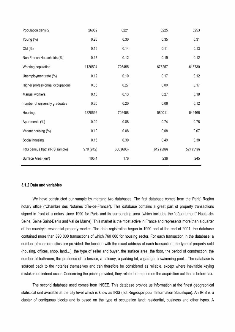
Population density 26082 8221 6225 5253
Young (%) 0.26 0.30 0.35 0.31
Old (%) 0.15 0.14 0.11 0.13
Non French Households (%) 0.15 0.12 0.19 0.12
Working population 1126504 726455 673257 615730
Unemployment rate (%) 0.12 0.10 0.17 0.12
Higher professionnal occupations 0.35 0.27 0.09 0.17
Manual workers 0.10 0.13 0.27 0.19
number of university graduates 0.30 0.20 0.06 0.12
Housing 1320696 702458 580011 549466
Apartments (%) 0.99 0.88 0.74 0.76
Vacant housing (%) 0.10 0.08 0.08 0.07
Social housing 0.16 0.30 0.49 0.38
IRIS census tract (IRIS sample) 970 (912) 606 (606) 612 (599) 527 (519)
Surface Area (km²) 105.4 176 236 245
3.1.2 Data and variables
We have constructed our sample by merging two databases. The first database comes from the Paris’ Region
notary office (“Chambre des Notaires d’Île-de-France”). This database contains a great part of property transactions
signed in front of a notary since 1990 for Paris and its surrounding area (which includes the “département” Hauts-de-
Seine, Seine Saint-Denis and Val de Marne). This market is the most active in France and represents more than a quarter
of the country’s residential property market. The data registration began in 1990 and at the end of 2001, the database
contained more than 890 000 transactions of which 760 000 for housing sector. For each transaction in the database, a
number of characteristics are provided: the location with the exact address of each transaction, the type of property sold
(housing, offices, shop, land…), the type of seller and buyer, the surface area, the floor, the period of construction, the
number of bathroom, the presence of a terrace, a balcony, a parking lot, a garage, a swimming pool... The database is
sourced back to the notaries themselves and can therefore be considered as reliable, except where inevitable keying
mistakes do indeed occur. Concerning the prices provided, they relate to the price on the acquisition act that is before tax.
The second database used comes from INSEE. This database provide us information at the finest geographical
statistical unit available at the city level which is know as IRIS (Ilôt Regroupé pour l’Information Statistique). An IRIS is a
cluster of contiguous blocks and is based on the type of occupation land: residential, business and other types. A
Residential IRIS has populations of 1800 to 5000 inhabitants and is homogeneous in respect of types of housing. A
Business IRIS clusters more than 1000 employees and has twice as many salaried jobs as resident inhabitants. Finally
Miscellaneous IRIS covers large areas and for special purposes (woods, parkland, docklands, cemeteries etc.)3 Paris and
its surrounding area is divided into 2 739 IRISes among which 94% are of residential type and 5% of business types.
The spatial distribution of the IRIS on the Metropolitan Area is showed in Map 1 and displayed a relatively homogeneous
pattern. The largest IRIS are generally not fully urbanized and covers by natural land. A large set of neighborhood
variables are available at the IRIS scale describing their socio-economic characteristics: population, density,
unemployment rate, professional group composition, population education level, immigrants. Census data on housing
conditions such as vacancy rate and building types are also available at the IRIS scale. IRIS data are only available for
the two last population census (in 1990 and in 1999) to date. As IRIS is the finest geographical statistical unit available at
the city level, we assimilate it as a neighborhood for the housing transactions. These areas are in fact small enough to be
considered as a “neighborhood” for households living there since in our sample the average neighborhood size is 0.27
km² (which is approximately 6 acres).
From these databases we extracted data for 1999 and after deleting incomplete records, missing data and
significant outliers, 21 000 housing transactions and 2 636 IRIS are available for our econometric analysis4. Summary
statistics for the explanatory variables are displayed in Table 2. The average apartment in our sample has a living space
of 53 m² with 2.46 rooms and one bathroom. It has been more frequently built between 1850 and 1947 than during the
other period and it has more frequently a lift and no garage. The average price is 2 394 € per m².
In the Metropolitan Area, the typical neighborhood is described by an average rate of employment of 11%, an
average percentage of 16% of non French households5, 33% of higher managements and professional occupations5, 24%
of intermediate occupations, 28% of clerical workers and 11% of manual workers5. The average density reaches 20 635
hab/km² (but with a very large standard deviation) and the percentage of vacant housing is 10% on average.
Table 2. Variables – Summary Statistics
Variables Description and Unit
Mean
(or nb*)
S.D.
( or %*)
STRUCTURAL ATTRIBUTES OF APARTMENTS (measured on the sample of transactions)
PRICE Transaction price in € m²(before tax) 2394.16 890.34
SURF Floor space (m2) 53.04 32.32
3 see INSEE [33] for more details. 4 For housing data, many observations have been deleted due to missing data for important structural attributes such as surface area or built period. For neighborhood, we delete all the IRIS having less than 227 inhabitants (227 is the value of the 5th percentile of the population distribution under which we consider that the IRIS is not relevant for a residential analysis purpose) and having no apartment. 5 For these variables, we note however that the variances are very large compared to the mean of the distributions.
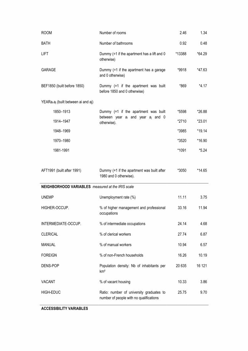
ROOM Number of rooms 2.46 1.34
BATH Number of bathrooms 0.92 0.48
LIFT Dummy (=1 if the apartment has a lift and 0
otherwise)
*13388 *64.29
GARAGE Dummy (=1 if the apartment has a garage
and 0 otherwise)
*9918 *47.63
BEF1850 (built before 1850) Dummy (=1 if the apartment was built
before 1850 and 0 otherwise)
*869 *4.17
YEARai-aj (built between ai and aj)
1850–1913
1914–1947
1948–1969
1970–1980
1981-1991
Dummy (=1 if the apartment was built
between year ai and year aj and 0
otherwise).
*5598
*2710
*3985
*3520
*1091
*26.88
*23.01
*19.14
*16.90
*5.24
AFT1991 (built after 1991) Dummy (=1 if the apartment was built after
1980 and 0 otherwise).
*3050 *14.65
NEIGHBORHOOD VARIABLES measured at the IRIS scale
UNEMP Unemployment rate (%) 11.11 3.75
HIGHER-OCCUP. % of higher management and professional
occupations
33.16 11.94
INTERMEDIATE-OCCUP. % of intermediate occupations 24.14 4.68
CLERICAL % of clerical workers 27.74 6.87
MANUAL % of manual workers 10.94 6.57
FOREIGN % of non-French households 16.26 10.19
DENS-POP Population density: Nb of inhabitants per
km²
20 635 16 121
VACANT % of vacant housing 10.33 3.86
HIGH-EDUC Ratio: number of university graduates to
number of people with no qualifications
25.75 9.70
ACCESSIBILITY VARIABLES
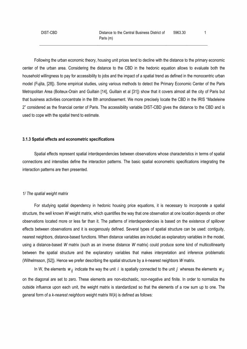
DIST-CBD Distance to the Central Business District of
Paris (m)
5963.30 1
Following the urban economic theory, housing unit prices tend to decline with the distance to the primary economic
center of the urban area. Considering the distance to the CBD in the hedonic equation allows to evaluate both the
household willingness to pay for accessibility to jobs and the impact of a spatial trend as defined in the monocentric urban
model (Fujita, [28]). Some empirical studies, using various methods to detect the Primary Economic Center of the Paris
Metropolitan Area (Boiteux-Orain and Guillain [14], Guillain et al [31]) show that it covers almost all the city of Paris but
that business activities concentrate in the 8th arrondissement. We more precisely locate the CBD in the IRIS “Madeleine
2” considered as the financial center of Paris. The accessibility variable DIST-CBD gives the distance to the CBD and is
used to cope with the spatial trend to estimate.
3.1.3 Spatial effects and econometric specifications
Spatial effects represent spatial interdependencies between observations whose characteristics in terms of spatial
connections and intensities define the interaction patterns. The basic spatial econometric specifications integrating the
interaction patterns are then presented.
1/ The spatial weight matrix
For studying spatial dependency in hedonic housing price equations, it is necessary to incorporate a spatial
structure, the well known W weight matrix, which quantifies the way that one observation at one location depends on other
observations located more or less far than it. The patterns of interdependencies is based on the existence of spillover
effects between observations and it is exogenously defined. Several types of spatial structure can be used: contiguity,
nearest neighbors, distance-based functions. When distance variables are included as explanatory variables in the model,
using a distance-based W matrix (such as an inverse distance W matrix) could produce some kind of multicollinearity
between the spatial structure and the explanatory variables that makes interpretation and inference problematic
(Wilhelmsson, [52]). Hence we prefer describing the spatial structure by a k-nearest neighbors W matrix.
In W, the elements ijw indicate the way the unit i is spatially connected to the unit j whereas the elements iiw
on the diagonal are set to zero. These elements are non-stochastic, non-negative and finite. In order to normalize the
outside influence upon each unit, the weight matrix is standardized so that the elements of a row sum up to one. The
general form of a k-nearest neighbors weight matrix W(k) is defined as follows:
*
*
*
( ) 0 if ,
( ) 1 if ( )
( ) 0 if ( )
ij
ij
ij
ij i
ij i
w k i j k
w k d d k
w k d d k
and * *( ) ( ) / ( )ij ij ij
j
w k w k w k
where ( )ijw k is an element of the standardized weight matrix and ( )id k is a critical cut-off distance defined for
each unit i. More precisely, ( )id k is the kth order smallest distance so that each unit i has exactly k neighbors. In the
paper, econometric results are obtained with k = 76.
2/ Spatial modeling of hedonic housing price functions
A spatial econometric model takes care of spatial dependencies as defined by W and through parametric
specifications allow to specify various forms of spatial autocorrelation.
Let's take as a starting point the general hedonic housing price model:
DNAP N(0 , ² I) [1]
where P is the ( 1)n vector of the housing prices, A is a ( )n j matrix of structural attributes of the apartment
(plus the constant), N is a ( )n t matrix of neighborhoods characteristics, D is a ( )n q matrix of accessibility
variables, , and are, respectively, j, t and q length vectors of unknown parameters to be estimated and is a random
error vector with the usual properties.
Following the hedonic modeling literature, we use the log-transformation on the dependent variable and on the
explanatory variables (the dummy variables excepted) so that estimated parameters can be interpreted as elasticities.
Following the spatial econometric literature (Anselin, [4]), two usual spatial models can be specified: a spatial lag
model (LAG) and a spatial error model (SEM). Both specifications seem possible a priori. In the LAG model, spatial
autocorrelation of observations is handled by the endogenous spatial lag variable WP and expresses the fact that the
price of an apartment is influenced by the price of the neighboring apartments. In the SEM model, we consider spatial
dependence as a statistical nuisance which may occur from various forms of misspecification. In this paper, spatial
dependence appears as a statistical nuisance which may stem from various forms of misspecification often at stakes in
hedonic housing models: omitted variables, lack of adequate neighborhood measures, etc. So we specify and estimate a
spatial error model (SEM).
The spatial error model is:
6 We have tested the presence of spatial autocorrelation with other k nearest neighbors matrices (k=10, k=15) to check the robustness of our results. Complete results are available upon request.

DNAP uW u N(0 , ² I) [2]
where is the scalar parameter expressing the intensity of spatial correlation between regression residuals.
Ignoring spatial dependence when it is present produces inefficient OLS estimators if model [1] is estimated by
OLS whereas [2] is the true model. The parameters of spatial models are generally estimated with the method of
Maximum likelihood (ML). In the case that estimates for is significant, spatial autocorrelation may be interpreted as a
spatial externality whose intensity depends on the estimated values of the parameters.

3.2 Empirical findings
All results are presented in Tables 3, 4 and 5 where the standard errors are corrected to take care of spatial
autocorrelation. Since our aim is to deal with the general impact of spatial dependence in the estimation of hedonic
housing price models, we have estimated equation [1] by OLS, performed different spatial tests and applied the
specification search approach defined by Anselin and Florax [6] to discriminate between the two forms of spatial
dependence : spatial autocorrelation of errors or endogenous spatial lag (the specification search approach is detailed in
Appendix). Spatial tests concluded that the appropriate specification is a Spatial Error Model (SEM) we then estimate by
the ML method. The impact of neighborhood effects is documented step by step to discriminate between social and
economic status of the neighborhood with the appropriate neighborhood variables.
3.2.1. Benchmark results
The core model takes into account the structural attributes of the apartments sold in 1999 and the accessibility to
the Central Business District of Paris. The estimates of the SEM hedonic housing price by ML are given in the second
column of Table 3. It appears that all coefficients are strongly significant and that a significance positive spatial
autocorrelation of the errors is found ( .0ˆ 670).
Regarding explanatory variables, the estimates are of expected signs. More precisely, price rises at a decreasing
rate with floor space since the elasticity is 0.026 and the unit price is lower for big apartments than for small ones. Looking
at the structural attributes, the impact of the number of bathrooms is positive and significant: an extra bathroom raises the
price by about 9.7% on average7. For all apartments, having been built before 1992 always lowers the prices. Very old
apartments (built before 1850) and apartments having been built between 1981 and 1991 have higher prices than
apartments having a construction date on the remaining period (between 1850 and 1970). These two periods correspond
to the lowest stocks of housing in the MA (see Table 2) and the the willingness to pay a premium may then reflect the
supply rationing on the associated housing sub-markets combined with household preferences for historical buildings or
modern buildings. The lowest unit prices are for a construction date between 1914 and 1969. As expected too, higher
apartments have higher prices and this positive impact is enhanced by the presence of a lift (+ 9% on average)
The impact of the local housing market, that is the number of transactions realized in the same neighborhood
during the year, is negative (but very small): increasing the number of transactions by 1% lowers the price by 0.032%.
This result is in line with a small trend in favor of a relaxation of the housing market with more successful transactions.
Finally, according to urban economic theories, a general decreasing spatial trend is found: the CBD distance gradient is
significant and negative and, other things being equal, price decreases at a decreasing rate with distance to the Central
7 Note that for a dummy variable, the percentage impact on the housing price of a change from 0 to 1, is calculated from the
corresponding estimated parameter ŝ as follows (Halvorsen and Palmquist, [32]): 100(exp(ŝ)-1).
Business District of the urban area. More precisely, if the distance to the CBD, in meters, increases by 1%, then the price
will decrease by 0.279%. This result confirms that accessibility to the primary core keep on exerting a global and strong
influence on the spatial pattern of housing prices in the Metropolitan Area of Paris.
Finally, regarding spatial effects, the estimated value ̂ of the spatial coefficient is significant which indicates that
housing prices are interdependent within the MA of Paris: what it occurs in one place depends on what it occurs in
neighborhing places through a spatial diffusion effect among housing price. As ̂ is positive, the spatial diffusion process
embodies positive spatial spillovers: good (resp. bad) surroundings value (resp. damage) housing prices8.
The core model in then extended to cope with the neighborhood effects issue and the impact of the economic and
social status of the neighborhoods on the housing prices.
3.2.2 Neighborhood effects
Following Rosenthal [47], we assume that neighborhood effects may be described by a small set of economic and
social characteristics of population and by housing policies. As the impact of neighborhood effects on housing values
relies on complex mechanisms, our strategy is to distinguish the economic side mechanism from the social side
mechanism and we estimate a specific model for each of them.
1/ The economic side of neighborhood effects
The economic effect relies on the economic profile and urban renewal policies and the estimated equation is
referred as the Economic Neighborhood Model.
Since the average income levels are not available at the IRIS scale in the population census tract, we approximate
the economic profile of the neighborhood with the percentage of residents in higher management and professional
occupations9 and with the percentage of residents in intermediate occupations. We test the impact of “income” mixity
against the impact of “income” specialisation with a socio occupational diversity index and a socio occupational
specialization index. Neighborhoods appear as specialized for high values of the specialization index while they are
considered as mixed for high values of the diversification index.
The impact of renewal policies is tested with two indexes measuring the building profile of the neighborhood. The
diversity construction index indicates mixed building profile while the specialization construction index indicates how
buildings of the main period are numerous compared to the building profile of the département. Finally, the percentage of
vacant housing controls for the obsolescence of housing and for the need of refurbishment in the neighborhood.
8 Such interpretations are conditioned by the fact that the Spatial Error Model is re-written in the Spatial Durbin Model (Le Gallo et al. [37]) 9 An alternative to the percentage of residents in higher management and professional occupations is the percentage of manual workers.

Table 3. Empirical results – Core model and economic neighborhood effects

Results are given in the third column of the table [3] for the economic profile (Economic Neighborhood Model) and
in the second column of the table [4] for the renewal policies profile (Economic and Renewal Neighborhood Model).
Table 4. Empirical results – Economic and social neighborhood effects
As expected the percentage of residents in higher management and professional occupations has a positive and
significant impact on the housing prices: when it increases by 1%, the unit price increases by 0.315%. On the contrary,
unit prices decrease with the percentage of residents in intermediate occupations (-0.17%). The impact of income mixity is
negative but with a small impact: a 1% more diversified socio-occupational profile in a neighborhood decreases the
housing price by 0.1%. The impact of income specialization is negative too with a stronger magnitude than for the
diversity. In fact, the interpretation of the last result is not obvious since the socio-occupational type is not a perfect proxy
of income. Moreover, the specialization index doesn’t indicate which socio-occupational group is the most represented in
the neighborhood. In fact, in urban studies, mitigated empirical results are often attached to the impact of specialization
external effects. Therefore, our findings show that neither specialization nor diversification value housing prices.
When the economic capital profile is supplemented by the impact of renewal policies in neighborhoods (Table [4]),
the model allows taking into account the impact of the building profile of the neighborhoods. Previous findings still hold
and the impact of the diversity index is positive: a 1% more diversified building structure increases housing unit price by
0.048%. On the contrary, specialization has a negative impact. As expected too, the percentage of vacant housing tends
to decrease the housing values. These results are in line with the neighborhood housing cycle model in favor of
gentrification process (Brueckner and Rosenthal, [16]).
2/ The social side of neighborhood effects
The social neighborhood effects depend on social profile, social externalities and social status. Social profile is
approximated by the percentage of young people, the percentage of old people, the presence of higher educated
individuals and the presence of no educated individuals. Social externalities are traditionally linked to the population
density and may follow a non monotonic trend. Finally, the social status is defined by the percentage of social housing
and the percentage of immigrants. Empirical results are presented in the table [4] and the table [5].
First, the presence of higher educated individuals is significant and positive with an elasticity of 0.356. On the
contrary and as expected, the presence of individuals with no qualification has a negative but small impact (- 0.059).
The impact of the age distribution of the population is positive for old people but negative for young people. Second, social
externalities have positive and greatest impacts in the most densely populated neighborhoods. These results are in favor
of a global positive impact of the social capital on housing values. Finally, the social status is of expected sign too and
confirms other empirical studies: an increase in the percentage of foreigners decreases the housing unit price as well as
an increase in the percentage of social housing.
Table 5. Empirical results – Social neighborhood effects

3/ The spatial dimension of neighborhood effects
Estimates of the spatial parameter ̂ are significant and positive in all Neighborhood Effects Models with a
magnitude between 0.407 and 0.632. As far as the Spatial Error Model is rewritten in the form of a Spatial Durbin Model,
spatial spillovers coming from neighborhood attributes are then at works in the Metropolitan Area of Paris and are
supported by the lagged exogenous variables as shown by the Spatial Durbin Model (Equation [3]):
u)DNA(WDNAWPP u N(0 , ² I) [3]
However, the spatial dimension of neighborhood effects is supported by the spatial interaction patterns defined by W and
in our case it is attached to a set of 7 nearest apartments for each housing i. The spatial dimension of neighborhood
effects is then probably confined to a small neighborhood area and may not take into account a larger spatial impact
coming from adjacent neighborhoods.
4. Conclusion
In this paper, hedonic housing price functions take into account both spatial effects and neighborhood effects. Our
results indicate that the inclusion of both accessibility variables and neighborhood attributes doesn't take all the spatial
effects into account. A spatial Error Model is then estimated. In addition, considering the fact that neighborhood variables
can be used to model the impact of neighborhood effects on housing values in the Metropolitan Area of Paris, we have
estimated several hedonic equations including the economic side and the social side of such neighborhood effects. Our
empirical results highlight the lumpy distribution of unit price along the general decreasing spatial trend from the Central
Business District once neighborhood effects have been introduced. Social capital, social status, social externalities and
urban renewal policies play local role and may positively or negatively impact the housing prices. We showed a positive
impact of diversified building patterns but a negative impact of social mixity which is somewhat conflictual but which is in
fact in line with many current questions about social segregation and spatial segregation in urban areas.
Our paper gives some preliminary results on the spatial dimension of neighborhood effects but this question has to
be further investigated with interactions patterns between neighborhoods themselves. In fact, only a small number of
empirical studies deals with this issue yet (Strange, [49]). Still, the heterogeneity issue has been not studied in the paper
while the spatial distribution of neighborhood attributes may display some spatial segregation patterns on which spatial
heterogeneity analysis could be based. These questions appear to be relevant to provide more evidence for relevant
urban renewal policies and will be part of our future research agenda.
References
[1] D. Aaronson. Neighborhood dynamics. Journal of Urban Economics, 49:1–31, 2001.
[2] A. Adair, J. Berry, S. McGreal, B. Deddis, and S. Hirst. Evaluation of investor behaviour in urban regeneration.
Urban Studies, 36(12):2031–2045, 1999.
[3] W. Alonso. Location and Land Use: Toward a General Theory of Land Rent. Harvard University Press, 1964.
[4] L. Anselin. Spatial Econometrics: Methods and Models, volume 1999. Kluwer Academic Publishers, 1998.
[5] L. Anselin. Spatial econometrics. In Companion to Econometrics, volume 1999. Oxford: Basil Blackwell, 2001.
[6] L. Anselin and R. Florax. Small sample properties of tests for spatial dependence in regression models, volume
1999, pages 146–176. Berlin: Springer, 1995.
[7] L. Anselin and J. Le Gallo. Interpolation of air quality measures in hedonic house price models: spatial aspects.
Spatial Economic Analysis, 1(1):32–52, 2006.
[8] S. Basu and T. G. Thibodeau. Analysis of spatial autocorrelation in house prices. Journal of Real Estate Finance
and Economics, 17:61–85, 1998.
[9] C. Baumont. Spatial effects of urban public policies on housing values. Papers in Regional Science, 2009. in press.
[10] C. Baumont, C. Ertur and J. Le Gallo. Spatial Analysis of Employment and Population Densities: The Case of the
Agglomeration of Dijon. Geographical Analysis 36 (2): 146-76, 2004
[11] C. Baumont and R. Guillain. Spatial patterns of cultural activities in the light of employment and population
suburbanisation: The case of Paris MA 1978; 1997. 53rd Regional Science Association International North
American Meeting (RSAI), Toronto, Canada, November. 2006
[12] C. Baumont and J. Le Gallo. Les nouvelles centralités urbaines, in : C. Baumont, PP Combes et H. Jayet,
Economie géographique: Les théories à l’épreuve des faits. pages 211 – 239. Economica, Paris, 2000.
[13] K. J. Beron, Y. Hanson, J. C. Murdoch and M. A. Thayer. Hedonic price functions and spatial dependence:
implications for the demand for urbain air quality, pages 267–281. Springer-Verlag, Berlin, 2004.
[14] C. Boiteux-Orain and R. Guillain. Changes in the intra-metropolitan location of producer services in Ile-de-France
(1978-1997): Do information technologies promote a more dispersed spatial pattern?, Urban Geography, 25, 550-
578, 2004.
[15] J. K. Brueckner. A vintage model of urban growth. Journal of Urban Economics. 8, 389-402, 1980
[16] J. K. Brueckner and S. S. Rosenthal. Gentrification and neighborhood housing cycles: will america's future
downtown be rich? Review of Economics and Statistics, 2008. forthcoming.
[17] J. K. Brueckner, J. F. Thisse, and Y. Zenou. Why is central Paris rich and downtown Detroit poor? an amenity-
based theory. European Economic Review, 43:91–107, 1999.
[18] A. Can and I. Megboluge. Spatial dependence and house price index construction. Journal of Real Estate Finance
and Economics, 14:203–222, 1997.
[19] J. L. Cumming and D. DiPasquale. The low-income housing tax credit: the first ten years. Housing Policy Debate,
10(2):257–267, 1999.
[20] J. L. Cumming, D. DiPasquale, and M. E. Kahn. Measuring the consequences of promoting inner city
homeownerships. Journal of Housing Economics, 11:330–359, 2002.
[21] D. M. Cutler, E. L. Glaeser, and J. L. Vigdor. The rise and decline of the american ghetto. Journal of Political
Economy, 107(3):455 –506, 1999.
[22] R. A. Dubin. Spatial autocorrelation and neighborhood quality. Regional Science and Urban Economics, 22:433 –
452, 1992.
[23] R. A. Dubin. Predicting house prices using multiple listings data. Journal of Real Estate Finance and Economics,
17(1):35–59, 1998.
[24] R. A. Dubin and C. H. Sung. Specification of hedonic regressions: non-nested tests on measures of neighborhood
quality. Journal of Urban Economics, 27:97–110, 1990.
[25] S.N. Durlauf. Neighborhood effects. in: J. V. Henderson & J. F. Thisse (ed.), Handbook of Regional and Urban
Economics, edition 1, volume 4, chapter 50, pages 2173-2242 Elsevier, 2004.
[26] R. Dye and D. P. McMillen. Teardowns and land values in the chicago metropolitan area. Journal of Urban
Economics, 61:45–63, 2007.
[27] G. Ellen, M. Schill, S. Susin, and A. Swartz. Building homes, reviving neighborhoods: Spillovers from subsidized
construction of owner occupied housing in New York city. Journal of Housing Research, 12(2):185–216, 2001.
[28] M. Fujita. Urban Economic Theory : Land Use and City Size, Cambridge University Press, Cambridge. 1999.
[29] M. Fujita and J. F. Thisse. Economie des villes et de la localisation. De Boeck. 2003.
[30] K. Gilley, T. Thibodeau, and S. Wachter. Anisotropic autocorrelation in house prices. Journal of Real Estate
Finance and Economics, 23:5–30, 2001.
[31] Guillain R., Le Gallo J., and Boiteux-Orain. Changes in spatial and sectoral patterns of employment in Ile-de-
France, 1978-1997. Urban Studies. 43(11). 2075-2098, 2006
[32] R. Halvorsen and R. Palmquist. The interpretation of dummy variables in semilogarithmic equations. The American
Economic Review, 70:474–475, 1980.
[33] INSEE. IRIS-2000: un nouveau découpage pour mieux lire la ville. Chiffres pour l’Alsace 43, 5, 2000.
[34] Y.M. Ioannides. Residential neighborhood effects. Regional Science and Urban Economics. 32: 145-165, 2002.
[35] Y.M. Ioannides and J.E. Zabel. 2008. Interactions, neighborhood selection and housing demand. Journal of Urban
Economics. 63: 229-252. 2008.
[36] M. S. Johnson and W. R. Ragas. CBD land values and multiple externalities. Land Economics, 63(4):335–347,
1987.
[37] J. Le Gallo, C. Ertur and C. Baumont. A spatial econometric analysis of convergence across European regions,
1980-1995. In B. Fingleton (eds) European regional growth, pages ,Berlin: Springer-Verlag. 2003.
[38] J. P. LeSage and R. K. Pace. Models for spatially dependent missing data. Journal of Real Estate Finance and
Economics, 29(2):233 –254, 2004.
[39] C.F. Manski. Economic Analysis of Social Interactions. Journal of Economic Perspectives, 14(3): 115-136, 2000.
[40] D. P. McMillen. Spatial autocorrelation or model misspecification? International Regional Science Review, 26:208 –
217, 2003.
[41] D. P. McMillen. Employment subcenters and home price appreciation rates in metropolitan Chicago, volume 18,
chapter Advances in Econometrics, Volume 18: Spatial and Spatiotemporal Econometrics, pages 237–257.
Elsevier, New York, 2004.
[42] R. K. Pace, R. Barry, and C. F. Sirmans. Spatial statistics and real estate. Journal of Real Estate Finance and
Economics, 17:5 –13, 1998.
[43] R. K. Pace and O. W. Gilley. Using the spatial configuration of the data to improve estimation. Journal of Real
Estate Finance and Economics, 14:333 – 340, 1997.
[44] A. Páez, T. Uchida, and K. Miyamoto. Spatial association and heterogeneity issues in land price models. Urban
Studies, 38(9):1493–1508, 2001.
[45] Y. Papageorgiou and H. Mullaly. Urban residential analysis: spatial consumer equilibrium. Environment and
Planning A, 8:489–506, 1976.
[46] W. A. Rabiega, T. W. Lin, and L. M. Robinson. The property value impact of public housing projects in low and
moderate density residential neighborhoods. Land Economics, 60(2):174–179, 1984.
[47] S. S. Rosenthal. Old homes, externalities, and poor neighborhoods: a model of urban decline and renewal. Journal
of Urban Economics, 63:816–840, 2008.
[48] S. Sheppard. Hedonic analysis of housing markets, volume 3, pages 1595 –1635. 1999.
[49] W. Strange. Overlapping neighborhoods and housing externalities. Journal of Urban Economics. 32: 17-39, 1991.
[50] W. R. Tolber. A computer movie simulating urban growth in the detroit region. Economic Geography, 46(2):234–
240, 1970.
[51] R. Y. C. Tse. Estimating neighbourhood effects in house prices: towards a new hedonic model approach. Urban
Studies, 39(7):1165 –1180, 2002.
[52] M. Wilhelmsson. Spatial models in real estate economics. Housing, Theory and Society, 19:92 –101, 2002.
[53] W. J. Wilson. The Truly Disadvantaged: The Inner City, the Underclass and Public Policy. University of Chicago
Press, Chicago, 1987.
[54] W. Yacovissi and C.R. Kern. Location and History as Determinants of Urban Residential Density. Journal of Urban
Economics. 38:207-220, 1995.
Appendix. Spatial error or spatial lag: a specification search approach
The classical “specific to general” specification search approach (Anselin and Florax, [6]) can then be applied to
determine the form taken by spatial autocorrelation, spatial lag, or spatial error. Recalling that the most usual test, Moran’s
I test adapted to regression residuals, indicates the presence of spatial dependence but not allow to discriminate between
the two forms of spatial dependence. For that purpose, four LM tests may be performed: respectively LMERR and LMLAG
and their robust versions, which have a good power against their specific alternative (Anselin [5]). The specification
search approach states that if LMLAG is more significant than LMERR and R-LMLAG is significant but R-LMERR is not,
then the appropriate model is the spatial autoregressive model. Conversely, if LMERR is more significant than LMLAG
and R-LMERR is significant but R-LMLAG is not, then the appropriate specification is the spatial error model.