Embed Size (px)
Citation preview

NAVAL POSTGRADUATE SCHOOL00 Monterey, California
i ot AVVO~DTICS ELECTE
fNOV 3 01993
ATHESIS
A METHODOLOGY FOR SOFTWARE COSTESTIMATION USING MACHINE LEARNING
TECHNIQUES
by
Michael A. KellyUeutenant, United States Navy
September, 1993
Thesis Advisor: Balasubramanium RameshCo-Advisor: Tarek K Abdel-Hamid
Approved for public release; distribution is unlimited.
93-2912098 11 29 014

REPORT DOCUMENTATION PAGE Fam Approved MB No. 0704
repfbswdm tar tu collectio owfadcgathon is emtzcd Wa &%cmW I howx par responic .nhkh the timc fr Wvew uIcs'q azscumak piw=# mi somm th do axtad imadodw~10gm wd revewsW the collubam of aarnmatao Sd comm-s re~wta tdo bwdm amtuc ar
alb w upa dth colleouma d arnioicmm. mbchg matiod for reh~ th h~ brdm. to Wadwoml Iudquwuni Savwm. Dw.eacrst for hionbu~ana. m Repma.c 1213 Jeffinm Dowu Mg~vu&y, Swtat 1204, Arhe~cm. VA 222M2-4302, ud to the Offimo of Mam~am mid Biad@K. Pqiawoek Re&Ajami
ed (07044133) WWma DC 20503.
1. AGENCY USE ONLY (Leave blank) 2. REPORT DATE 3. REPORT TYPE AND DATES COVERED
13 S1p 993 Master's Thesis, Final
* TITLE AND SUBTITLE A Methodology for Software Cost Estimation 5. FUNDING NUMBERSUsing Machine Learning Techniques
. AUTHOR(S) Michael A. Kelly
. PERFORMING ORGANIZATION NAME(S) AND ADDRESS(ES) S. PERFORMING ORGANIZATIONNaval Postgraduate School REPORT NUMBERMonterey CA 93943-5000
. SPONSORING/MONrrORING AGENCY NAME(S) AND ADDRESS(ES) 10. SPONSORING/MIONITORINGI AGENCY REPORT NUMBER
11. SUPPLEMENTARY NOTES The views expressed in this thesis are those of the author and do not reflect thefficial policy or position of the Department of Defense or the U.S. Government.
12a. DISTRIBUTION/AVAILABILITY STATEMENT 12b. DISTRIBUTION CODEpproved for public release; distribution is utlimitedI A
13. ABSTRACT (maximum 200 words)The Department of Defense expends billions of dollars on software development and maintenance annually.
any Department of Defense projects fail to be completed, at large monetary cost to the government, due toe inability of current software cost-estimation techniques to estimate, at an early project stage, the level ofor required for a project to be completed. One reason is that current software cost-estimation models tend
o perform poorly when applied outside of narrowly defined domains.Machine learning offers an alternative approach to the current models. In machine learning, the domainecific data and the computer can be coupled to create an engine for knowledge discovery. Using neural
etworks, genetic algorithms, and genetic programming along with a published software project data set,everal cost estimation models were developed. Testing was conducted usi.g a separate data set. All threeechniques showed levels of performance that indicate that each of these techniques can provide softwareroject managers with capabilities that can be used to obtain better software cost estimates.
14. SUBJECT TERMS Software cost estimation, neural networks, genetic algorithms, 15. NUMBER OF PAGESenetic programming, machine learning, software project managemet, COCOMO, 143
cial intelligence 16. PRICE CODE
17. SECURITY 18. SECURITY 19. SECURITY 20. LIMITATION OFCLASSIFICATION OF CLASSIFICATION OF CLASSIFICATION OF ABSTRACTREPORT THIS PAGE ABSTRACT UL
Unclassified Unclassified UnclassifiedNSN 7540-01-280-5500 Standard Form 298 (Rev. 2-9)
Prmamiedby ANSI SU1. 239-18
• - . .I I I I I I I I I IIII ,

Approved for public release; distribution is unlimited.
A Methodology for Software Cost Estimation Using Machine Learning Techniques
by
Michael A. Kelly
Lieutenant, United States NavyB.S., Tulane University, 1983
Submitted in partial fulfillment
of the requirements for the degree of
MASTER OF SCIENCE IN INFORMATION TECHNOLOGY MANAGEMENT
from the
NAVAL POSTGRADUATE SCHOOL
September 1993
Author: Kelly
Approved by: ,tvi 14
Balasubramanium Ramesh, Thesis Advisor
Tarek Abdel-Hamid, Thesis Co-Advisor
David R. %"iple, "•
Department of Administrative ience
ii

ABSTRACT
The Department of Defense expends billions of dollars on software development and
maintenance annually. Many Department of Defense projects fail to be completed, at
large monetary cost to the government, due to the inability of current software
cost-estimation techniques to estimate, at an early project stage, the level of effort
required for a project to be completed. One reason is that current software
cost-estimation models tend to perform poorly when applied outside of narrowly-defined
domains.
Machine learning offers an alternative approach to the current models. In machine
learning, the domain specific data and the computer can be coupled to create an engine for
knowledge discovery. Using neural networks, genetic algorithms, and genetic
programming along with a published software project data set. several cost estimation
models were developed. Testing was conducted using a separate data set. All three
techniques showed levels of performance that indicate that each of these techniques can
provide software project managers with capabilities that can be used to obtain better
software cost estimates. Accesion For
NTIS CRA&I
DTIC TAB []"UnannouncedJu--tficat!on
E
By......................By ............................................
Dist, ibution I
Av\):,-b4Iy Code..
... ... Avail a;rd I or... O~~Dst ", :ia
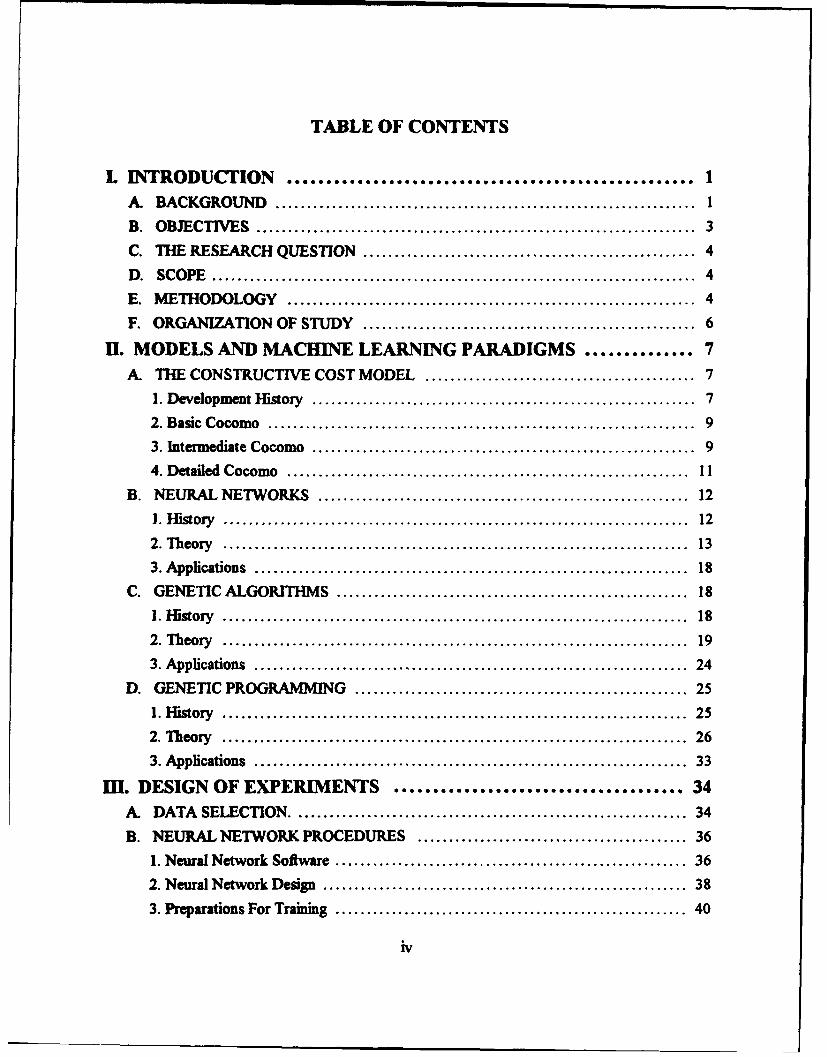
TABLE OF CONTENTS
L INTRODUCTION .................................................... 1A. BACKGROUND ................................................................... I
B. OBJECTIVES ...................................................................... 3
C. THE RESEARCH QUESTION ..................................................... 4
D . SCO PE ............................................................................. 4
E. METHODOLOGY ................................................................. 4
F. ORGANIZATION OF STUDY ..................................................... 6
H1. MODELS AND MACHINE LEARNING PARADIGMS .............. 7A. THE CONSTRUCTIVE COST MODEL ........................................... 7
1. Development History ............................................................. 7
2. Basic Cocom o ................................................................... 9
3. Intermediate Cocomo ............................................................. 9
4. D etailed Cocom o ................................................................ II
B. NEURAL NETWORKS ......................................................... 12
1. H istory ......................................................................... 12
2. Theory ......................................................................... 13
3. Applications .................................................................... 18
C. GENETIC ALGORITHMS ........................................................ 18
1. H istory ......................................................................... 18
2. Theory .......................................................................... 19
3. Applications .................................................................... 24
D. GENETIC PROGRAMMING .................................................... 25
1. H istory ......................................................................... 25
2. Theory .......................................................................... 26
3. Applications .................................................................... 33
II. DESIGN OF EXPERIMENTS ..................................... 34A. DATA SELECTION ............................................................. 34
B. NEURAL NETWORK PROCEDURES ......................................... 36
1. Neural Network Software ........................................................ 36
2. Neural Network Design ......................................................... 38
3. Preparations For Training ........................................................ 40
iv

4. Automating The Training Process ................................................ 41C. GENETIC ALGORITHM PROCEDURES ....................................... 46
I. Genetic Algorithm Goal ......................................................... 46
2. Genetic Algorithm Software .................................................... 46
3. Gaucsd Preparation .............................................................. 47
4. Initial Genetic Algorithm Benchmarking .......................................... 48
5. Genetic Algorithm Constraints ................................................... 51
6. The Genetic Algorithm Testing Process ......................................... 52
D. GENETIC PROGRAMMING PROCEDURES ................................... 53
1. Genetic Programming Software ................................................ 53
2. Genetic Programming Preparation ............................................... 54
IV. ANALVSIS OF RESULTS ........................................... 59A. MEASURES OF PERFORMANCE .............................................. 59
B. NEURAL NETWORKS .......................................................... 60
1. First Phase Results .............................................................. 60
2. Second Phase Results ........................................................... 63
3. Neural Network Structural Analysis ............................................. 65
C. GENETIC ALGORITHMS ....................................................... 68
1. First Phase Results .............................................................. 68
2. Second Phase Results .......................................................... 72
3. Genetic Algorithm Structural Analysis .......................................... 73
D. GENETIC PROGRAMMING .................................................... 76
1. First Phase Results .............................................................. 76
2. Second Phase Results ........................................................... 78
3. Genetic Program Structural Analysis ........................................... 81
V. CONCLUSIONS AND RECOMMENDATIONS ..................... 84A. CONCLUSIONS ................................................................. 84
B. RECOMMENDATIONS FOR FURTHER RESEARCH ........................... 87
APPENDIX A ..... .... ... ............................... ...... ...... 89APPENDIX B . ........................... .............................. 92
APPENDIX C ......................................................... 93
APPENDIX D .......................................................... 94APPENDIX E .............. ............................................ 97
V
APPENDIX F ......................................................... 111
APPENDIX G ......................................................... 116
LIST OF REFERENCES ................................................ 135
INITIAL DISTRIBUTION LIST ....................................... 136
vi

1. INTRODUCTION
A. BACKGROUND
The use of computers and computing technology within the Department of Defense
continues to grow at an accelerating rate. As the use of computers has expanded, so has
the need for computer software. While computer hardware has decreased in cost relative
to its performance, the cost of software continues to increase. It is estimated that the
Department of Defense spends approximately thirty billion dollars annually in the
acquisition and maintenance of software (Boehm, 1987, pg. 43). Virtually no area within
the military has escaped the "software invasion." From the million-plus lines of code for
the Seawolf submarine's BSY-2 computer system to the two million lines of code in the
Navy's NALCOMIS Phase HI logistics system, software is now one of the driving factors
in the success of the United States military.
Although the technology used to develop software has improved through the use of
such methods as object-oriented programming and computer-aided software engineering
(CASE), one software management area which remains underdeveloped is software cost
estimation. Since the greatest expense in a software development effort is manpower,
software cost estimation models focus on estimating the effort required to complete a
particular project. This estimate of effort required can then be translated into dollars using
the appropriate labor rates. The current cost estimation models available to software
project managers fail to provide sound estimates in a consistent manner, even within their

own narrowly defined domains. Improper estimation of costs is a major reason why many
Department of Defense software projects have failed. With a decreasing budget for
defense, it is of even greater necessity that managers have available to them effective
software cost estimation tools.
There are many models available for software cost estimation. One of the more
popular models is the Constructive Cost Model, or COCOMO, developed by Barry
Boehm while at TRW (Boehm, 1981, pg. 493). This model is based on a database of
sixty-three projects developed at TRW during the 1960's and 1970's and is described in
detail in Boehm's book, Software Engineering Economics. Part of the reason for the
popularity of COCOMO is that it is relatively easy to apply and it resides in the public
domain. Other models, such as ESTIMACS, developed by Howard Rubin and currently
the property of Computer Associates, Inc., are proprietary due to the nature of the project
data from which they were developed. A common thread that exists in all of these models
is that they were developed by domain experts and are heavily dependent upon the
judgement of the expert for the determination of the model inputs and relationships
extracted from the software project data.
An alternative approach to model development that can reduce the need for the
domain expert to act solely on judgement is through the use of artificial intelligence (Al),
specifically the use of machine learning, While artificial intelligence has been a subject of
study since the 1950's, it has periodically been greeted with skepticism for a perceived
inability to deliver at the level of performance promised by its proponents. In recent years,
2
as both computer hardware and software have grown more powerful and the objectives of
Al have been better defined, the fitld of artificial intelligence has seew a resurgence.
Techniques are now available that have the ability to provide solid results over a range of
problems when appropriately applied. An area of great activity today in artificial
intelligence is machine learning. Knowledge acquisition and classification is a very labor
intensive task. The computer, with its ability to toil without time off for vacations or
holidays, provides a natural platform for the automation of the knowledge acquisition
process, or to at least serve as an assistant in the knowledge acquisition process. The
application of machine learning to the problem of software cost estimation is the focus of
this investigation.
B. OBJECTIVES
Current methodologies for software cost estimation vary widely in their estimates
when presented with identical inputs (Kemmerer, 1987, pg. 416). A common
characteristic of most cost estimation models is that they tend to provide only marginally
useful results within a rigid domain that is often too narrow to be of use when pursuing
new types of software development projects. The emphasis of this thesis is to develop a
methodology for the application of machine learning techniques to software cost
estimation. The three machine learning techniques cli- sen for this project are neural
networks, genetic algorithms, and genetic programming. The performance of the models
derived from each machine-learning technique are evaluated and compared with respect to
ease of application, accuracy, and extensibility. Additionally, the models are analyzed to
3

see what insight they can provide into the relative importance of the available input
variables.
C. THE RESEARCH QUESTION
The primary research question of this thesis is to determine the feasibility of applying
machine learning to the problem of software cost estimation. This research uses the
COCOMO data set for model training and the COCOMO and Kemmerer data sets for
testing the resulting models. The other important questions of this thesis are to determine
the effectiveness of machine-learning techniques when applied to the cost estimation
problem and what insight, if any, can be gained from the machine generated models into
cost-estimation.
D. SCOPE
The scope of this thesis is to apply the three machine learning techniques to the cost
estimation problem using the COCOMO and Kemmerer data sets and to determine the
extent to which they are appropriate and insightful to the cost estimation process. The
scope of this thesis is not to develop to develop a better model for cost estimation but
instead to develop a methodology for the application of machine learning to this problem.
E. METHODOLOGY
This thesis is divided into four steps. First, the sixty-three projects in the COCOMO
data set are analyzed and partitioned into training and testing data sets. Secondly, the
three machine learning techniques are applied using the training data set as the means for
knowledge acquisition. The resulting models are then tested using the COCOMO data not
4
included in the training set. A variety of parameters and constraints specific to each
technique are varied. In a second iteration of this process, all of the 63 COCOMO
projects are used as the training set, and a second set of 15 projects, identical to the set
used by Kemmerer in his 1987 article in the Communications of the ACM is used as the
testing set. The goal of this sequence of training and testing is to see how well the various
machine generated models can perform across different software development domains.
Since the fifteen projects presented by Kemme;'er were developed outside of TRW, which
is where Boehm's data was obtained, the capability of the models to generalize can be
tested.
In the case of neural networks, multiple network configurations are tested. The
resulting trained neural networks are ranked on overall performance against actual project
effort and against each other.
In the third step of this thesis, a genetic algorithm is applied to the training data uwing
the original COCOMO model structure as a fitness function template in order to obtain a
revised COCOMO parameter set. These new values will be used to evaluate the testing
data using the Intermediate COCOMO model structure. Initially, the genetic algorithm is
relatively unconstrained. In further tests, constraints are added to the genetic algorithm
fitness finction to determine the effect on the resulting model parameters and on the
model's accuracy with respect to the testing data.
Finally, the relatively new concept of genetic programming is applied to the training
data set to see what algorithmic models for cost estimation can be derived purely from the
5

training data with no preconceived functional form or structure provided. The resulting
models will again be tested using the test data set.
The resulting models from all techniques will also be analyzed to see what insights, if
any, they provide into the overall cost estimation process. The way that the various input
variables are used by the machine generated models may provide an opportunity to
discover relationships previously unnoticed. This is an additional benefit of using the
computer in the knowledge acquisition process and it is explored.
F. ORGANIZATION OF STUDY
Chapter I provides a general background for this study. Chapter U discusses the
COCOMO model and the three machine learning techniques in greater detail, including
some history and the basic principles of each. Chapter E] describes the experimentation
process and setup. Chapter IV discusses the results of the various experiments and
compares these results with those obtained using the original COCOMO model in its
various forms. Additional insights into the cost estimation question will be noted and
analyzed at this time. Chapter V is the conclusions and recommemdations resulting from
this inquiry.
6
H. MODELS AND MACHINE LEARNING PARADIGMS
A. THE CONSTRUCTIVE COST MODEL1. Development History
The Constructive Cost Model, commonly referred to as COCOMO, was
developed by Barry Boehm in the late 1970's, during his tenure at ITRW, and published in
1981 in his text, Software Engineering Economics. This model, which is actually a
hierarchy of three models of increasing detail, is based on a study of sixty-three projects
developed at TRW from the period of 1964 to 1979. In his text, Boehm describes the
development of COCOMO as being the result of a review of then available cost models
coupled with a Delphi exercise that resulted in the original model This model was
calibrated using a database of 12 completed projects.
When that model failed to provide a reasonable explanation of project variations
when expanded to a 56 project database, the concept of multiple development modes was
added. Three development modes were defined as organic, semidetached, and embedded.
Organic mode refers to relatively small (< 50 KDSI) stand-alone projects with
non-rigorous specifications that typically use small development teams and involve low
risk. Organic mode projects are usually thought to have higher levels of productivity than
the other two modes due to their small size and flexibility in specifications. Semidetached
mode refers to projects of small to medium size (up to 300 KDSI) that involve
characteristics of both organic and embedded projects, such as a system that has some
7

rigorous specifications and some non-rigorous specifications. Embedded mode refers to
projects of all sizes that typically have rigorous, non-negotiable specifications that are
tightly coupled to either hardware, regulations, operational procedures, or a combination
of these factors. Embedded mode projects generally require innovative architectures and
algorithms and entail greater risk than organic or semidetached projects of similar size.
(Boehm, 1981, pp. 76-77)
Once the three development modes were defined, they were calibrated using the
original 56 project database to provide greater accuracy. Seven more projects were later
added to the project database for a total of sixty-three. Appendix A contains the entire
database. Boehm describes COCOMO as not being heavily dependent on statistical
analysis for calibration due to the inherently complex nature of software development.
Instead, COCOMO relies on empirically derived relationships among the various cost
drivers. These cost drivers are related to attributes associated with the product being
developed, the target computer platform, the development personnel, and the development
environment. (Boehm, 1981, pg. 493)
The COCOMO model is popular since it is easy for managers to apply and it is
widely taught in software management courses. In his text, Boehm provides clear
definitions of the model inputs through a variety of tables and charts. This type of
presentation allows managers to understand what costs the model is estimating and how
the estimates are reached. Therefore, the model can also be used by managers to perform
8

sensitivity analyses to examine tradeoffs on a variety of different software development
issues. (Boehnm, 1984, pg 13)
2. Basic COCOMO
Basic COCOMO is the simplest version of the model It is designed to provide
a macro level scaling of project effort based on the mode of development and the
projected size of the project in thousands of delivered source instructions (KDSI). Boehm
describes its accuracy as limited though, due to the lack of factors to account for
differences in project attributes, such as hardware constraints and personnel experience.
(Boehm, 1981, pg. 58) The three equations for Basic COCOMO are:
Table 2-1 Basic COCOMO Effort Equations
Mode Effort
Organic MM=2.4(KDSI)' 0O
Semidetached MM=3.O(KDSI)11 2
Embedded MM=3.6(KDSI)' 20
The accuracy of Basic COCOMO is only satisfactory. For the sixty-three
projects in the database, Basic COCOMO estimates are within a factor of 1.3 of the
actuals just 29% of the time and within a factor of 2 of the actuals just 60% of the time.
(Boehm, 1981, pg. 84)
3. Intermediate COCOMO
Intermediate COCOMO tries to improve upon the accuracy of Basic COCOMO
by introducing the concept of cost drivers, which act as effort multipliers. Fifteen factors
have been identified by Boehm as attributes that affect the effort required on a particular
9
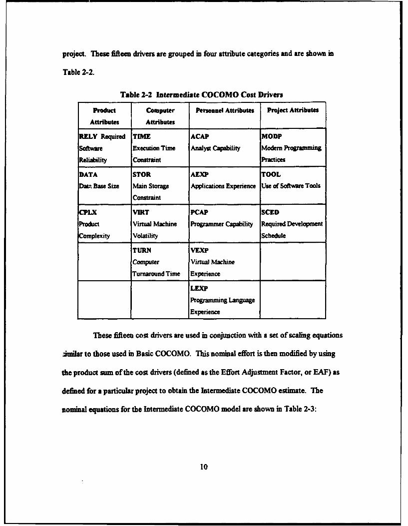
project. These fifteen drivers are grouped in four attribute categories and are shown in
Table 2-2.
Table 2-2 Intermediate COCOMO Cost Drivers
Product Computer Personnel Attributes Project Attributes
Attributes Attributes
RELY Required TIME ACAP MODP
Software Execution Time Analyst Capability Modem Programming
Reliability Constraint Practices
DATA STOR AEXP TOOL
Dat Base Size Main Storage Applications Experience Use of Software Tools
Constraint
CPLX VIRT PCAP SCED
Product Virtual Machine Programmer Capability Required Development
Complexity Volatility Schedule
TURN VEXP
Computer Virtual Machine
Turnaround Time Experience
LEXP
Programming Language
Experience
These fifteen cost drivers are used in conjunction with a set of scaling equations
imilar to those used in Basic COCOMO. This nominal effort is then modified by using
the product sum of the cost drivers (defined as the Effort Adjustment Factor, or EAF) as
defined for a particular project to obtain the Intermediate COCOMO estimate. The
nominal equations for the Intermediate COCOMO model are shown in Table 2-3:
10
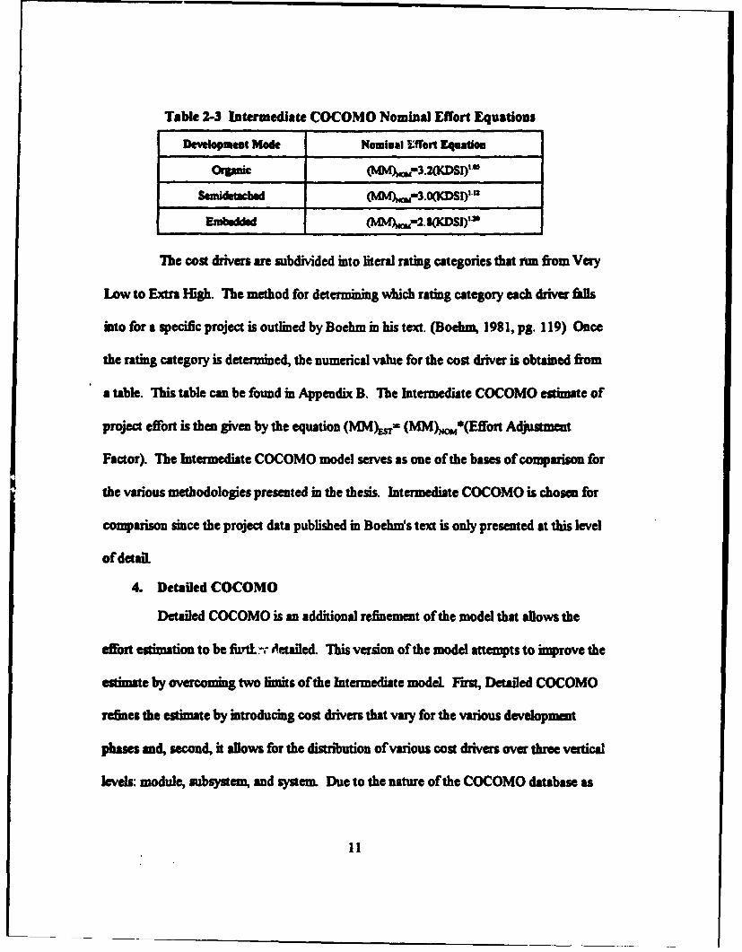
Table 2-3 Intermediate COCOMO Nominal Effort Equations
Development Mode Nominal Offort Equation
Ormnic (MM -3.2(KDSI)'"
Semidetached (MM)-3.0(DSI)1'U
Embedded M) -2.8(CDSD)'3
"The cost drivers are subdivided into literal rating categories that ran from Very
Low to Extra High. The method for determining which rating category each driver fils
into for a specific project is outlined by Boehm in his text. (Boehm, 1981, pg. 119) Once
the rating category is determined, the numerical value for the cost driver is obtained from
a table. This table can be found in Appendix B. The Intermediate COCOMO estimate of
project effort is then given by the equation (MM)ýss= (MM)*(Effort Adjustment
Factor). The Intermediate COCOMO model serves as one of the bases of comparison for
the various methodologies presented in the thesis. Intermediate COCOMO is chosen for
comparison since the project data published in Boehm's text is only presented at this level
of detail.
4. Detailed COCOMO
Detailed COCOMO is an additional refinement of the model that allows the
effwt estimation to be futL- Acetailed. This version of the model attempts to improve the
estimate by overcoming two limits of the Intermediate model. Frst, Detailed COCOMO
refines the estimate by introducing cost drivers that vary for the various development
phases and, second, it allows for the distribution of various cost drivers over three vertical
Levels: module, subsystem, and system. Due to the nature of the COCOMO database as
11
presmted in Boelhm's text, the Detailed version of the model will not be used as the basis
of comparison during the evaluation of the various machine learning paradigms. (Boehm,
1981, pp. 344-345)
EL NEURAL NETWORKS1. History
The neural network paradigm has a colorful history dating back to the 1950Ys.
This paradigm grew out of the efforts of early artificial intelligence (AI) researchers to
construct systems that mimicked the actions of neurons in the human brain. In 1958,
Frank Rosenblatt published a paper that defined a neural network structure called a
perceptron (Eberhart, 1990, pg. 18). This paper outlined the principles that information
could be stored in the form of connebtions and that information stored in this manner
could be updated and refined by the addition of new connections. This research laid the
foundation for both types of training algorithms, supervised and unsupervised, that are
used in neural networks today.
While work continued in the neural network field during the 1960's and 1970's
their usefulness was in doubt until the publication of a paper by John Hopfield, ftom the
California Institute of Technology (Eberhart, 1990, pg. 29). Hopfield's work was
important because he identified network structures and algorithms that could be defined in
a general nature and he was the first to identify that networks could be implemented in
electronic circuitry, which interested semiconductor manufacturers. The publication in
1986 of Parallel Distributed Processing by the Parallel Distributed Processing Research
12

Group ensured the rebirth of neural networks by describing in great detail a variety of
architectures, attributes and transfer functions (Eberhan, 1990, pg. 32). Since then, the
variety and application of neural networks have grown immensely. The Defense
Advanced Research Projects Agency sponsored a neural network review in 1988 and
published a report on the field (Maren, 1990, pg. 20). This publication tended to validate
the field as being worthy of research funding and now there are a variety ofjournals and
publications dedicated to this field, as well as an international society (Maren, 1990, pg.
20).
2. Theory
There are a wide variety of neural network models in use today. One of the
most common networks, and the one chosen for use in this thesis, is the backpropagation
network. In this case, backpropagation refers to the training method used for this
network. The network in operation acts in a feed-forward manner. The basic principle of
operation is simple. A backpropagation network is typically constructed of an input layer
of neurons, an output layer ofneurons, and one or more hidden layers of neurons. Bias
neurons may also be defined for each hidden layer. Each neuron (or node) is defined by a
transfer function. In the case of the backpropagation network, the flmction usually has a
sigmoid or S-shape that ranges asymptotically between zero and one. The reason for
choosing the sigmoid is that the function must be continuously differentiable and should be
asymptotic for infinitely large positive and negative values of the independent variables.
(Maren, 1990, pg. 93) The neurons in each layer are then assigned a weighted connection
13
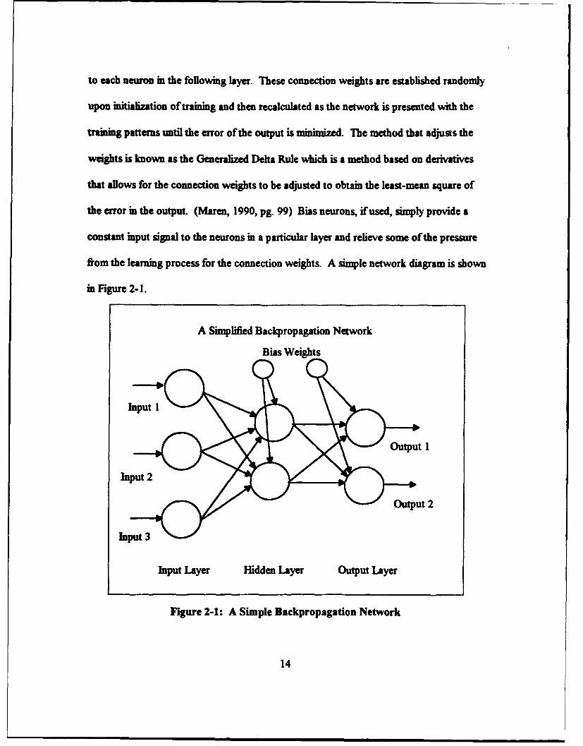
to each neuron i the following layer. These connection weights are established randomly
upon initialization of training and then recalculated as the network is presented with the
training patterns until the error of the output is minimized. The method that adjusts the
weights is known as the Generalized Delta Rule which is a method based on derivatives
that allows for the connection weights to be adjusted to obtain the least-mean square of
the error in the output. (Maren, 1990, pg. 99) Bias neurons, if used, imply provide a
constant input signal to the neurons in a particular layer and relieve some ofthe pressure
from the learning process for the connection weights. A simple network diagram is shown
in Figure 2-1.
A Simplified Backpropagation Network
Bias Weights
S~Output 2
Inpu 3
Input Layer Hidden Layer Output Layer
Figure 2-1: A Simple Backpropagation Network
14

A backpropagation network is capable of generalizing and feature detection
because it is trained with different examples whose features become embedded in the
weights of the hidden layer nodes (Maren, 1990, pg. 93). An example of the operation of
a neural network is provided by Maren and involves a neural network designed to solve an
XOR classification problem. The diagram for this network showing the configuration at
initialization and upon completion of training is shown in Figure 2-2 (Maren, 1990, pg.
97).
The example given by Maren is a version of the backpropagation network in
which each hidden layer neuron can have a threshold value which is added to sum of the
inputs to that neuron before the application of the sigmoid transfer function. These
threshold values are found using the same Delta rule that is used to find the connection
weights. During the training process, the connection weights (and threshold values) are
adjusted using the following equation:
w*,g) = w td) + Ca * Delta(wyad) - output activation_level
where w, stands for the new and old values of the connection weight between node i and
node j, and ca is a constant that defines the magnitude of the effect of Delta on the weight.
Delta descnibes a function that is proportional to the negative of the derivative of the error
with respect to the connection weight and outputactivation level is the output of the jth
neuron. This backpropagation of error mechanism allows the weights at all layers to be
adjusted as the training process is performed, including any connections between hidden
layer neurons. (Maren, 1990, pp. 100-101)
15

Initialization with Random Convergence to StableWeights and Threshold Values Weights and Thresholds
After Training Interactions
.093 -6.56
".413 .850 13.34 13.13
.909 •-.441• -11.62 -'13.13
Initial Results: Results After TrainingInput Output Input Output(0,0) 0.590 (0,0) 0.057(0,1) 0.589 (0,1) 0.946(1,0) 0.589 (1,0) 0.949(1,1) 0.601 (1,1) 0.052
]Figure 2-2 A Neural Network Example of an XOR Problem (Maren, 1990)
16
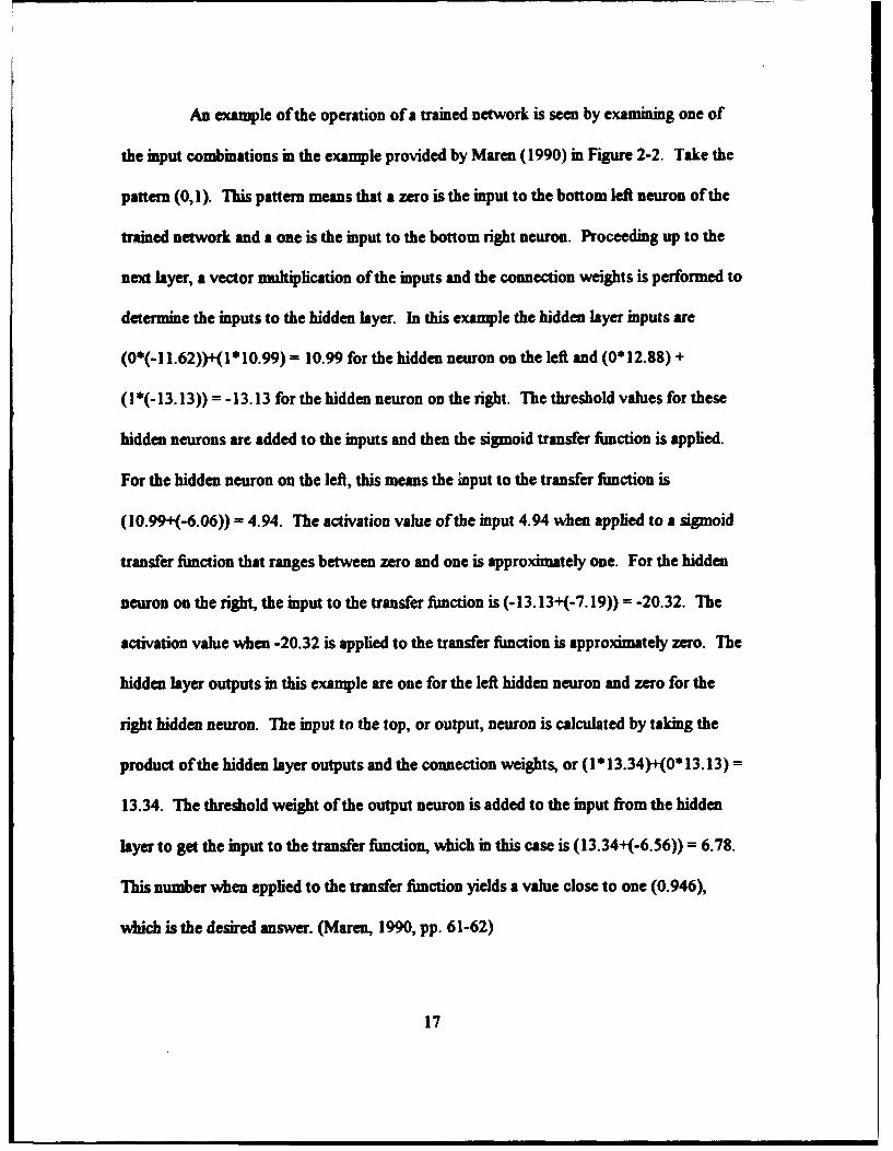
An example of the operation of a trained network is seen by examining one of
the input combinations in the example provided by Maren (1990) in Figure 2-2. Take the
pattern (0,1). This pattern means that a zero is the input to the bottom left neuron of the
trained network and a one is the input to the bottom right neuron. Proceeding up to the
next layer, a vector multiplication of the inputs and the connection weights is performed to
determine the inputs to the hidden layer. In this example the hidden layer inputs are
(0*(-1 1.62))+(1"10.99) = 10.99 for the hidden neuron on the left and (0"12.88) +
(1*(-13.13)) = -13.13 for the hidden neuron on the right. The threshold values for these
hidden neurons are added to the inputs and then the sigmoid transfer function is applied.
For the hidden neuron on the left, this means the input to the transfer function is
(10.99+(-6.06)) = 4.94. The activation value of the input 4.94 when applied to a sigmoid
transfer finction that ranges between zero and one is approximately one. For the hidden
neuron on the right, the input to the transfer function is (-13.13+(-7.19)) = -20.32. The
activation value when -20.32 is applied to the transfer function is approximately zero. The
hidden layer outputs in this example are one for the left hidden neuron and zero for the
right hidden neuron. The input to the top, or output, neuron is calculated by taking the
product of the hidden layer outputs and the connection weights, or (1"13.34)+(0*13.13) =
13.34. The threshold weight of the output neuron is added to the input from the hidden
layer to get the input to the transfer function, which in this case is (13.34+(-6.56)) = 6.78.
This number when applied to the transfer function yields a value close to one (0.946),
which is the desired answer. (Maren, 1990, pp. 61-62)
17
3. Applications
Neural networks are currently being used in a variety of applications. Some of
the major uses are in the areas of filtering, image and voice recognition, financial analysis,
and forecasting (Zahedi, 1991, pg. 27). Commercial neural network software is available
from a variety of vendors. Specialized programmable hardware boards that contain
chipsets that can mimic the operation of a neural network are also available for very
intensive neural network applications. The neural networks in this thesis were developed
using a product from California Scientific Software, Inc. called Brainmaker.
C. GENETIC ALGORITHMS1. History
Nature's capability to find solutions for complex problems through the process
of natural selection has fascinated researchers fo- generations. The ability of organisms to
adapt to their environment by altering their characteristics through mating, which provides
an opportunity for gene crossover as well as an occasional genetic mutation, has proven to
be a powerful technique of problem solving. Genetic algorithms were an outgrowth of
early work during the 1950's and 1960's that attempted to combine computer science and
evolution with the hope of creating better programs. In the mid 1960's, John Holland
developed the first genetic algorithms that could be used to represent the structure of a
computer program as well as perform the mating, crossover, and the mutation processes.
Since then, genetic algorithms have grown in popularity and have been applied to a wide
variety of problems, especially in the field of engineering design, where optimization
18

involving large numbers of independent variables is a common situation. (Holland, 1992,
pg. 66)
2. Theory
Genetic algorithms are in the simplest definition another method for search and
optimization. However, they differ from traditional methods such as hill-climbing and
random walks in at least four ways (Goldberg, 1989, pg. 7). First, genetic algorithms use
codings of the various parameters in a function, not the actual function parameters
themselves. This coding usually consists of fixed-length strings of characters that are
patterned after chromosomes. Each string, or chromosome, then has a fitness value
associated with it which is a measure of how well it performs in terms of the criteria
defined for the problem. Second, genetic algorithms perform highly parallel searches
using a population of points vice a single point. Third, genetic algorithms use the
objective function, or actual payoff information, to determine fitness instead of derivatives
or other information. This capability separates the genetic algorithm from those techniques
that require gradient information about the fimction to perform their searches. Instead,
the genetic algorithm has the capability to work wirh the actual function itself. Finally,
genetic algorithms use probabilistic rules to make shifts from on. generation to the next
instead of deterministic rules. (Goldberg, 1989, pp. 7-10)
The easiest way to understand the working of the genetic algorithm is to see it in
action. In the following example, similar to the Hamburger Problem presented by Koza
(1992, pg. 18), the genetic algorithm is used to maximize a function. The coding of
19
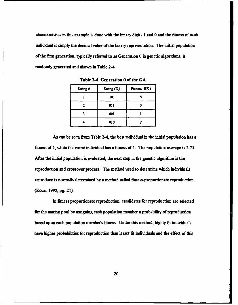
characteristics in this example is done with the binary digits I and 0 and the fitness of each
individual is simply the decimal value of the binary representation. The initial population
of the first generation, typically referred to as Generation 0 in genetic algorithms, is
randomly generated and shown in Table 2-4.
Table 2-4 Generation 0 of the GA
String # String (s) Fitness fR)
1 101 5
2 011 3
3 001 1
4 010 2
As can be seen from Table 2-4, the best individual in the initial population has a
fitness of 5, while the worst individual has a fitness of 1. The population average is 2.75.
After the initial population is evaluated, the next step in the genetic algorithm is the
reproduction and crossover process. The method used to determine which individuals
reproduce is normally determined by a method called fitness-proportionate reproduction
(Koza, 1992, pg. 21).
In fitness proportionate reproduction, candidates for reproduction are selected
for the mating pool by assigning each population member a probability of reproduction
based upon each population member's fitness. Under this method, highly fit individuals
have higher probabilities for reproduction than lesser fit individuals and the effect of this
20
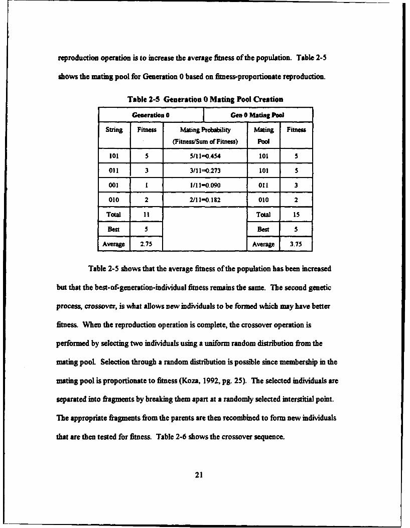
reproduction operation is to increase the average fitness of the population. Table 2-5
shows the mating pool for Generation 0 based on fitness-proportionate reproduction.
Table 2-5 Generation 0 Mating Pool Creation
Generation 0 Gen 0 Mating POoW
String Fitness Mating Probability Mating Fitness
(Fitness/Sum of Fitness) Pool
101 5 5/11-0.454 101 5
Ol 3 3/11=0.273 101 S
001 1 1/11=0.090 011 3
010 2 2/111=0.182 010 2
Total I I Total 15
Best 5 Best 5
Average 2.75 Average 3.75
Table 2-5 shows that the average fitness of the population has been increased
but that the best-of-generation-individual fitness remains the same. The second genetic
process, crossover, is what allows new individuals to be formed which may have better
fitness. When the reproduction operation is complete, the crossover operation is
performed by selecting two individuals using a uniform random distribution from the
mating pool Selection through a random distribution is possible since membership in the
mating pool is proportionate to fitness (Koza, 1992, pg. 25). The selected individuals are
separated into fragments by breaking them apart at a randomly selected interstitial point.
The appropriate fragments from the parents are then recombined to form new individuals
that are then tested for fitness. Table 2-6 shows the crossover sequence.
21
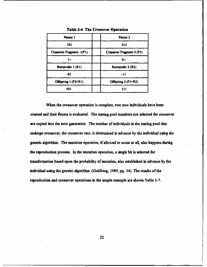
Table 2-6 The Crossover Operation
Parent I Parent 2
101 011
Crossover Fragment I(FI) Crossover Fragment 2 (P2)
1- 0-
Remainder I (RI) Remainder 2 (R2)
-01 -II
Offspring I (F2+RI) Offspring 2 (F1+R2)
001 111
When the crossover operation is complete, two new individuals have been
created and their fitness is evaluated. The mating pool members not selected for crossover
are copied into the next generation. The number of individuals in the mating pool that
undergo crossover, the crossover rate, is determined in advance by the individual using the
genetic algorithm. The mutation operation, if allowed to occur at all, also happens during
the reproduction process. In the mutation operation, a single bit is selected for
transformation based upon the probability of mutation, also established in advance by the
individual using the genetic algorithm. (Goldberg, 1989, pg. 14) The results of the
reproduction and crossover operations in the simple example are shown Table 2-7.
22
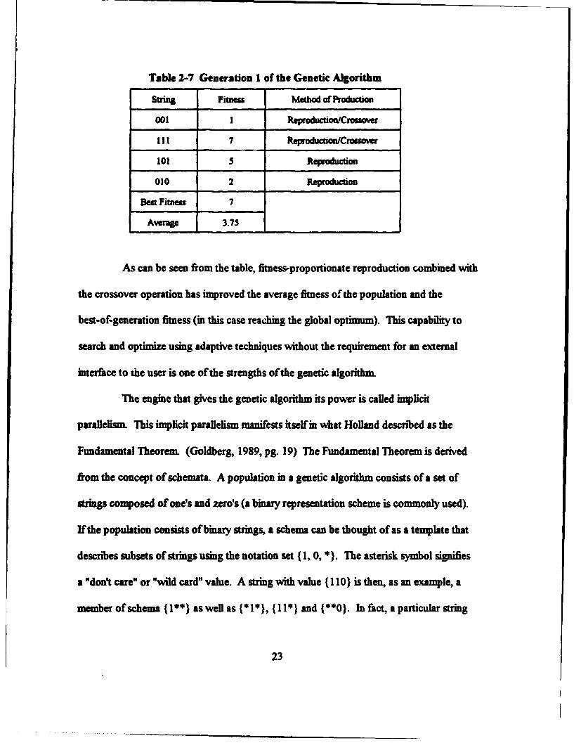
Table 2-7 Generation I of the Genetic Algorithm
Suting Fitness Method of Production
001 1 Reproduction/Crosamw
111 7 Reproduction/Crossover
101 5 Reprodc-on
010 2 Reproduction
Best Fitness 7
Averae 3.75
As can be seen from the table, fitness-proportionate reproduction combined with
the crossover operation has improved the average fitness of the population and the
best-of-generation fitness (in this case reaching the global optimum). This capability to
search and optimize using adaptive techniques without the requirement for an external
interface to the user is one of the strengths of the genetic algorithm.
The engine that gives the genetic algorithm its power is called implicit
parallelism. This implicit parallelism manifests itself in what Holland described as the
Fundamental Theorem. (Goldberg, 1989, pg. 19) The Fundamental Theorem is derived
from the concept of schemata. A population in a genetic algorithm consists of a set of
strings composed of one's and zero's (a binary representation scheme is commonly used).
If the population consists of binary strings, a schema can be thought of as a template that
describes subsets of strings using the notation set ( 1, 0, *). The asterisk symbol signifies
a "don't care" or "wild card" value. A string with value (110) is then, as an example, a
member of schema (1"*) aswell as (*1*), (11*) and {**0). In fact, a particular string
23

in a population is a member of 26'* schema. A schema can be thought of as
representing certain characteristics of a candidate solution to the fitness function. As
populations of strings (or chromosomes) proceed from one generation to the next through
the process of reproduction and crossover, individuals with greater fitness rise in number
at the expense of lesser fit individuals. Schemata behave in a similar manner. A schema
(or characteristic set) grows at a rate proportional to the average fitness of that particular
schema over the average fitness of the population. A schema whose average fitness is
above that of the population average will be represented in greater numbers in the
succeeding generations. A schema whose average fitness is less than the population
average will see its numbers diminish. In fact, above average schema will see their
numbers increase in an exponential manner in succeeding populations. This effect of
simultaneously increasing the fitness of the population and promoting the exponential
growth of beneficial schemata (or characteristics) through the reproduction operation,
coupled with the crossover operation that creates population diversity through an orderly
exchange of characteristics is what gives the genetic algorithm its implicitly parallel nature.
(Goldberg, 1989, pp. 29-33)
3. Applications
The use of genetic algorithms has increased greatly in the past few years as
people have realized rhe benefits they bring to certain types of problems that have resisted
solution by more traditional methods. In one case genetic algorithms were used to
develop control mechanism for a model of a complex set of gas pipelines that transport
24

natural gas across a wide area. Having only various compressors and valves with which to
control the gas flow, and with a large time lag between any action and reaction, this
problem had no standard analytic solution. A genetic algorithm was developed by David
Goldberg at the University of Illinois that was capable of "learning" the control procedure.
In another case, Lawrence Davis used genetic algorithms to design communications
networks that maximized data flow with a ninimum number of switches and transmission
lines. General Electric is currently using genetic algorithms in the design of new
commercial turbofan engine components. Using a genetic algorithm, General Electric
engineers were able to reduce the time required to improve the design of an engine turbine
from weeks to days. This is notable since there are at least 100 variables involved in a
turbine design as well as a large number of constraints. (Holland, 1992, pg. 72-73)
Goldberg's text lists additional uses of genetic algorithms ranging from medical imaging to
biology to the social sciences (Goldberg, 1989, pg. 126). There are currently several
conferences, both national and international, devoted to the discussion of genetic
algorithms.
D. GENETIC PROGRAMMING
1. History
Genetic programming is an exciting new field in computing pioneered by John
Koza of Stanford University in the late 1980's. Koza, in his text Genetic Programming:
On the Programming of Computers by Means of Natural Selection, describes the core
concept of his technique as being the search for a computer program of a given fitness
25
from the space of all possible computer programs using the tools of natural selection. This
approach is different from more traditional artificial intelligence techniques in that for any
particular problem using traditional techniques, such as neural networks, the goal is
usually to discover a specialized structure that provides a certain output given certain
inputs. Koza reframes this statement by saying what we truly want to discover is a certain
computer program that will produce the desired output from a given set of inputs. Once
the problem is refrained as that of finding a highly fit program within the space of all
possible programs, the problem is reduced to that of space search. (Koza, 1992, pg.2)
The technique of genetic programming is not the first attempt at using
computers to try to generate programs. Researchers since the 1950's have attempted
using various methods to generate programs ranging from blind random search to asexual
reproduction and mutation. More recently, researchers in the genetic algorithm field have
attempted to use genetic algorithms to generate programs by using ever more specialized
chromosome representation schemes or by using a special type of genetic algorithm
known as a classifier system to generate programs based on if-then rules (Koza, 1992, pp.
64-66). Koza is the first researcher, however, to develop an appropriate representation
scheme and methodology for applying natural selection techniques to the problem of
program generation.
2. Theory
The concept of a "highly fit" computer program as a solution to a particular
problem is disturbing to most people at first. We are accustomed to the idea of a
26
computer program being either "right" or "wrong" when applied to a particular problemn
Koza counters this sentiment and other similar sentiments by saying that the process of
natural selection is neither "right" nor "wrong" but that nature supports many different
approaches to the same problem, all of which have a certain "fitness". The key to natures
approach, according to Koza, is that form follows fitness (Ko7a, 1992, pp. 1-7 ). The
requisite tools used in Koza's approach are a well-defined function representation scheme,
a method for generating an initial random population of programs, a fitness measurement
technique, and a procedure for applying genetic operations to the members of the
population.
The representation schenme chosen by Koza for genetic programming is based on
a type of structure known as a symbolic expression, or S-expression. Since this type of
structure is a key component of the programming language LISP, this language was
chosen as the platform for developing genetic programming. It is not a requirement to use
this language for genetic programming, but it has many features that facilitated the
development of this technique. (Koza, 1992, pp. 70-71) An example of a LISP
S-expression is shown in Figure 2-3.
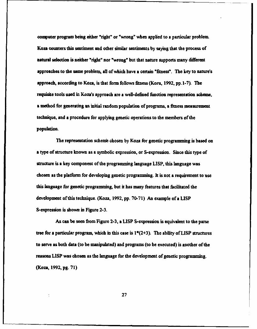
As can be seen from Figure 2-3, a LISP S-expression is equivalent to the parse
tree for a particular program, which in this case is 1"(2+3). The ability of LISP structures
to serve as both data (to be manipulated) and programs (to be executed) is another ofthe
reasons LISP was chosen as the language for the development of genetic programming.
(Koza, 1992, pg. 71)
27

Figure 2-3 A LISP S-expression
In genetic programming, these LISP S-expressions are composed of structures
that are derived from a predefined function set and terminal set. The function set consists
of whatever domain-specific functions the user feels are sufficient to solve the problem
and the terminal set is the arguments that the functions are allowed to take on (Koza,
1992, pg. 80). For instance, the function set may be comprised of mathematical,
arithmetic, or boolean operators while the terminal set is usually comprised of variables
from the problem domain and an unspecified integer or floating-point random constant.
Since it is impossible to determine in advance what the structures will look like, it is
necessary to ensure in advance that each function possesses the property of closure (Koza,
1992, pg. 81). The closure property requires that the allowable arguments for any
function be well-defined in advance to prevent the function from taking illegal arguments.
While this may seem like an imposing task, it is usually not a serious problem and is easily
rectified by prior planning of the function definitions. As an example, division by zero is
undefined. If the division operator is a member of the function set, then by defining a
28

special division operator in advance that handles this special case, it is possible to ensure
closure on this function. (Koza, 1992, pg. 82)
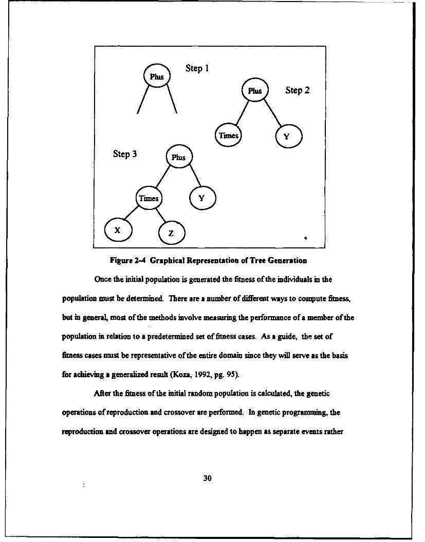
Once the representation scheme is defined, the initial program structures can be
generated (Koza, 1992, pg 91). In Koza's method, the initial structures are generated
randomly using a combination of two techniques, "full" and "grow". The root, or
beginning, of one of the LISP S-expressions, or trees, is always a function, since a root
that consisted of a terminal would not be capable taking any arguments. Once the root
function is selected, a number of lines, equivalent to the number of arguments the function
requires, are created which radiate away from the flmction. The endpoints of these lines
are then filled by a selection from the combined set of fimctions and terminals. If another
function is selected as an endpoint, the selection process continues onward until the
endpoints consist of terminals. There is a preset maximum depth that trees may attain.
The terms "full" and "grow" as mentioned above refer to the depth of the trees. In the
"full" method, all trees filled until they are at the specified maximum depth. In the "grow"
method, the trees are of variable depth. In practice, Koza recommends an approach called
"ramped half-and-half' that combines these two approaches (Koza, 1992, pp. 91-92).
Koza additionally recommends that each structure generated for the initial random
population be checked for uniqueness to ensure a range of diversity of genetic material
(Koza, 1992, pg. 93). Figure 2-4 gives a graphical representation of the creation of an
individual in the initial population.
29
$\Step I
x 2
Figure 2-4 Graphical Representation of Tree Generation
Once the initial population is generated the fitness of the individuals in the
population must be determined. There are a number of different ways to compute fitness,
but in general, most of the methods involve measuring the performance of a member of the
population in relation to a predetermined set of fitness cases. As a guide, the set of
fitness cases must be representative of the entire domain since they will serve as the basis
for achieving a generalized result (Koza, 1992, pg. 95).
After the fitness of the initial random population is calculated, the genetic
operations of reproduction and crossover are performed. In genetic programming, the
reproduction and crossover operations are designed to happen as separate events rather
30

than as parts of a two-step process as with the genetic algorithm. Reproduction occurs by
copying an S-expression from one generation to the next. Candidates for reproduction
are selected by using the fitness-proportionate method or a second method known as
tournament selection. In tournament selection, a specified number of population members
are randomly selected with replacement. The individual with the best fitness is then
reproduced in the next generation. The sampling with replacement is what ensures that
fitter individuals survive into succeeding generations. (Koza, 1992, pg. 100)
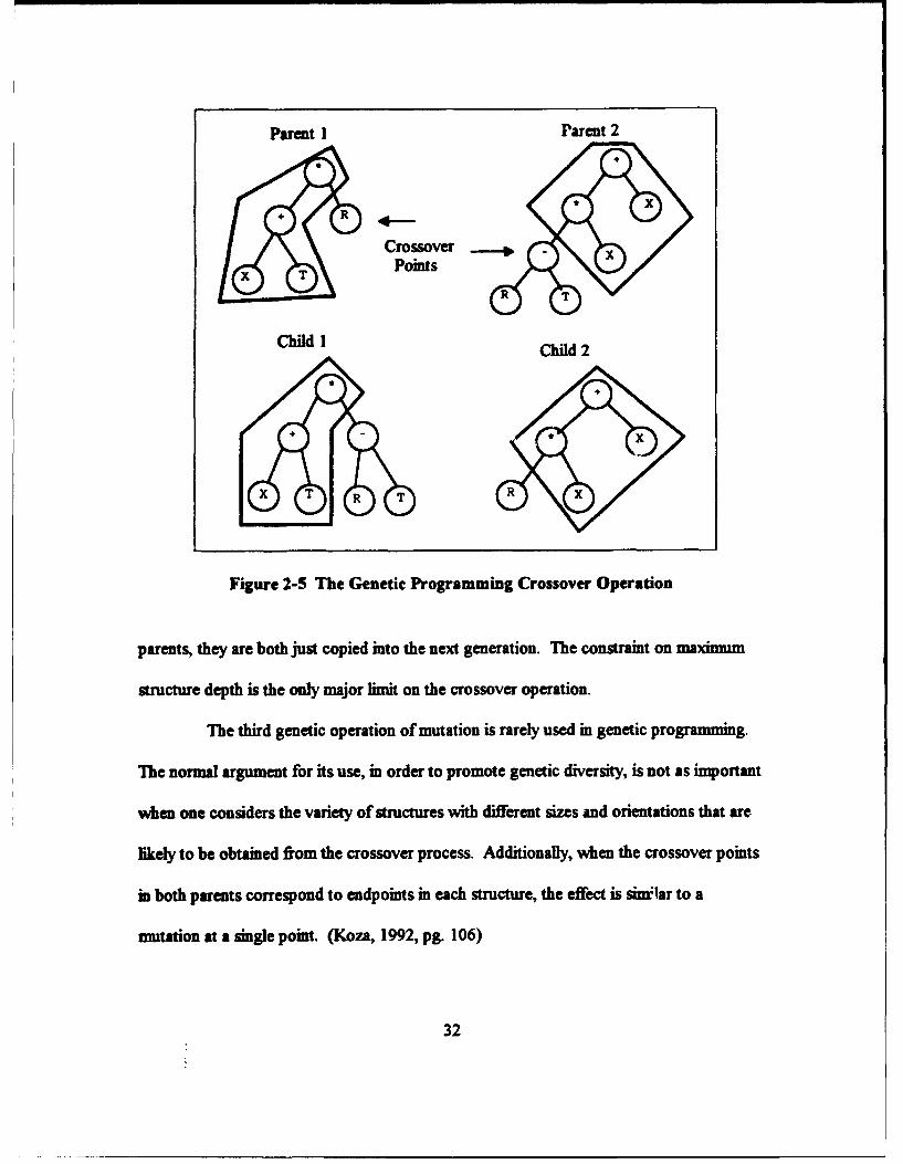
The crossover operation in genetic programming is more complex than that of
the genetic algorithm due to the differences in the structure of the population members.
The crossover candidates are selected using the same method chosen for reproduction.
This ensures that crossover occurs between individuals in a manner proportionate to their
fitness. After two individuals have been selected a separate random number is chosen for
each individual which corresponds to a point in each structure. It is at these points that
the crossover operation takes place by swapping subtrees, (Koza, 1992, pg. 101) Figure
2-4 shows an example of the crossover operation. The previously described property of
closure on the fimction set ensures that any resulting S-expressions will be legitimate
program representations. Since the points selected for crossover are most likely to be at
difi-rent levels in each structure there are a variety of situations that may result. (Koza,
1992, pg. 103) An individual may reproduce with itself and produce two totally new
structures. If the crossover point happens to be at the root of on S-expression, that entire
S-expression will become a subtree on the other parent. If the root is selected in both
31
Parent 1 Parent 2
xR 4
Crossover -*
X T PointsR P
Child I Child 2
X T R T
Figure 2-5 The Genetic Programming Crossover Operation
parents, they are both just copied into the next generation. The constraint on maximum
structure depth is the only major limit on the crossover operation.
The third genetic operation of mutation is rarely used in genetic programming.
The normal argument for its use, in order to promote genetic diversity, is not as important
when one considers the variety of structures with different sizes and orientations that are
likely to be obtained from the crossover process. Additionally, when the crossover points
in both parents correspond to endpoints in each structure, the effect is sim'lar to a
mutation at a single point. (Koza, 1992, pg. 106)
32
3. Applications
Due to its relative youth as, technique, applications usiLg genetic programming
are currently confined to mostly experimental problems. Koza does present in his text a
copious amount of examples of applying his technique to a wide range of problems,
including symbolic regression, game playing strategies, decision tree induction, and
artificial life (Koza, 1992, pg. 12-14). In each case, a domain specific function set with
the proper closure was determined in advance. Once the function set and the appropriate
fitness measure was specified, all of the problems proceeded in the identical manner using
a domain-independent implementation of the mechanical operations of evolution. An
initial population was generated at random and the genetic operations of reproduction and
crossover were used to create succeeding generations. Koza was able to show via
empirical methods that genetic programming succeeded in each case to find a solution that
satisfied the appropriate fitness measure (Koza, 1992, pg. 4). This ability to solve
problems over a wide variety of domains by using a domain-independent method for
searching the space of possible computer programs to find an individual computer
program is what makes genetic programming an exciting new method of discovery (Koza,
1992. pg. 8).
33
MI. DESIGN OF EXPERIMENTS
A. DATA SELECTION.
The COCOMO data set used for training and testing the machine learning techniques
examined in this thesis is drawn from pages 496 and 497 of Boehm's book, Software
Engineering Economics. The sixty-three projects used to develop the three versions of
COCOMO are summurized in this data base. This data includes the project type, year
developed, the dev.elopment language, the values of the 15 cost drivers, the development
mode, and the various COCOMO estimates. The Kemmerer project data was provided by
the author in electronic form and is included in Appendix C. The experimental approach
taken for each machine-learning technique consisted of a two-step process that required a
different training and testing data set for each step. The first step used only the
COCOMO data partitioned into training and testing data sets. The second step consisted
of using the COCOMO data for training and the Kemmerer data for testing. The
partitioning of the COCOMO data set in the first step required two tradeoff
considerations.
The first tradeoff involved the size of the training and testing data sets. Machine
learning methods perform at their best when they have a large amount of data available for
training that is representative of the population, or problem domain. In fact a good
guideline is more is always better. However, there are only 63 projects available in the
COCOMO data base in the text. In this case, choosing to use too much data for training
34

reduces the number of data sets available for testing and trivializes the results beyond a
certain point. Alternatively, choosing too little data for training reduces the effectiveness
of the machine learning techniques. A balance was struck by deciding to break the data
into thirds, with two-thirds to be used for training and one-third to be used for testing.
This was accomplished by transcribing the data set from the text into a Quattro Pro
spreadsheet and then sorting the projects by size and type. Once the data was sorted in
this manner, a random number between one and three was assigned to each project. The
data was then partitioned into groups based on the random number assigned and each
group was analyzed. This cursory analysis showed that for each group the mean project
size in thousands of delivered source instructions (KDSI), the average year of
development, and the development mode proportions were roughly similar, indicating a
reasonable distribution. After this analysis, 42 of the projects were identified as the
training set and 21 projects were identified as the testing set. These data sets are included
in Appendix D. The same training and testing sets were then used for aU of the machine
learning techniques examined. The composition of the training and testing data sets for
each set of experiments was also kept as identical as possible and consisted of the project
size, annual adjustment factor, development mode, and the fifteen COCOMO cost drivers,
with limited exceptions.
One effect of partitioning the data in this manner is that the testing data set may not
be completely characteristic of the "population". Some testing set projects contained
some cost driver values that were not contained in the training data set. This situation
35
describes the second tradeoff Hand selecting the data to ensure that every cost driver
value represented in the data base was in the training set was initially considered but
rejected for two reasons. First, it would probably be meaningless when considering that
there are, at a minimum, four values for each cost driver. For fifteen cost drivers this
means there are at least 4" possible combinations of cost drivers, and there are only 63
projects in our data set. Secondly, on a more practical basis, several of the cost driver
values are only represented onc,. in the project data base, so if they were included in the
training data there would be no way of examining the effectiveness of this measure.
Therefore, there appeared to be no benefit in ensuring that every cost driver value was
filly represented in the training set.
B. NEURAL NETWORK PROCEDURES
1. Neural Network Software
The software used to develop the neural networks in this thesis is BrainMaker
Professional v2.5, which is designed and marketed by California Scientific Software, Inc.
This software is a DOS-based product manufactured for use on IBM-compatible personal
computers. BrainMaker is designed to construct, train, test, and run backpropagation
neural networks. It is a menu-driven program that provides the user a large range of
control over the design and operation of a neural network. BrainMaker comes with an
extensive manual as well as a companion program called NetMaker which can be used to
prepare the data files needed by BrainMaker. All of the files used by BrainMaker are in
standard ASCII format, so they can be prepared using most any text editor if the user so
36

desires, although using the NetMaker program speeds up the process since it helps
automate the generation of BrainMakers inputs.
BrainMaker requires two files at a minimum to train. The first file is the
network definition file, which tells BrainMaker the key network parameters, such as the
number of input and output neurons, the number of hidden layers and hidden neurons, the
input and output data definitions and ranges, the learning rate, and the type of transfer
function the neurons will use. An example of a network definition file is shown in Figure
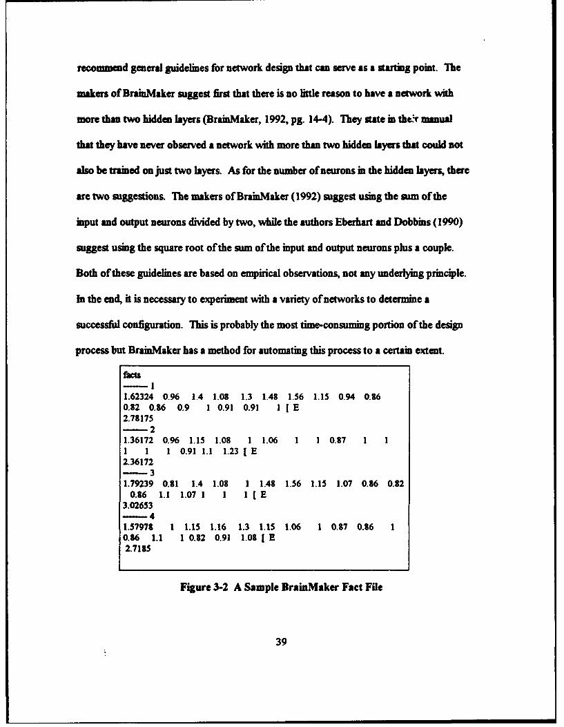
3-I. The second file that BrainMaker requires is the fact file. This is the file that contains
the data the network will use for training. This file consists of alternating rows of data,
with the first row representing one input set and the second row representing one output
set. An example of a fact file is contained in Figure 3-2. Additional input files that may be
included are a testing fact file and a running fact file. The testing fact file consists of
alternating rows of input and output data not included in the training fact file. This data
may be used during the training process to judge the prospective performance of the
network at user-defined intervals during the training process. When a testing fact file is
specified, BrainMaker pauses at the specified interval and tests the current network
configuration using the facts in the testing fact file. The results of these tests along with
some associated error statistics are written to an output file. The training statistics for
each run may also be written to a separate file if this option is activated. The running fact
file provides the user with the capability to test the trained network with new sets of inputs
in a batch manner and write the results to an output file in a user-specified format.
37
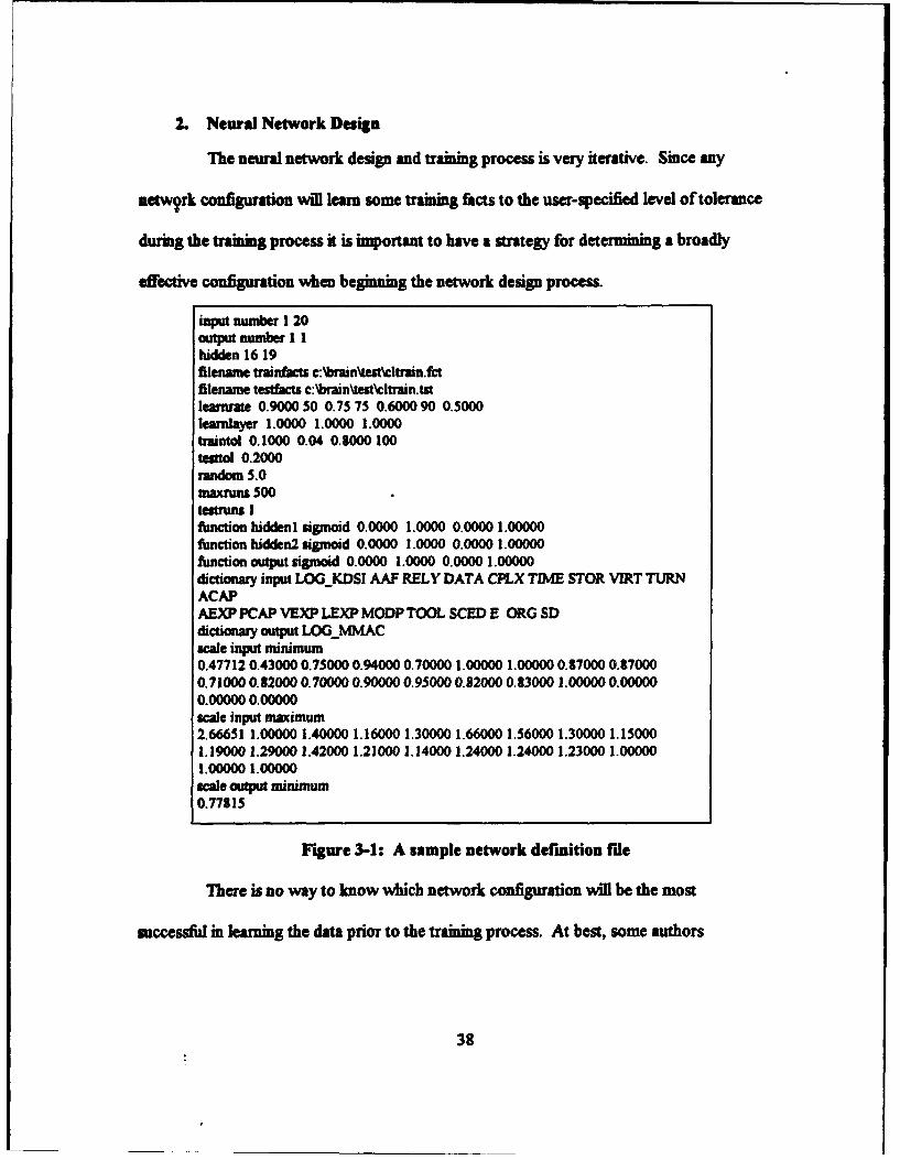
2. Neural Network Design
The neural network design and training process is very iterative. Since any
netw?rk configuration will learn some training facts to the user-specified level of tolerance
during the training process it is important to have a strategy for determining a broadly
effective configuration when beginning the network design process.
input number 1 20output number I 1hidden 16 19filename trainficts c:Wbaintest~ltrain.fctfilename testfacts c:b\rain\testtcltrain.tstlearnrate 0.9000 50 0.75 75 0.6000 90 0.5000learnlayer 1.0000 1.0000 1.0000traintol 0.1000 0.04 0.8000 100temol 0.2000random 5.0nmaxruns 500testruns Ifunction hiddenI siSmoid 0.0000 1.0000 0.0000 1.00000function hidden2 sigmoid 0.0000 1.0000 0.0000 1.00000function output sigmoid 0.0000 1.0000 0.0000 1.00000dictionary input LOGKDSI AAF RELY DATA CPLX TIME STOR VIRT TURNACAPAEXP PCAP VEXP LEXP MODP TOOL SCED E ORG SDdictionary output LOQJVIMACscale input minimum0.47712 0.43000 0.75000 0.94000 0.70000 1.00000 1.00000 0.37000 0.870000.71000 0.82000 0.70000 0.90000 0.95000 0.82000 0.83000 1.00000 0.000000.00000 0.00000"scale input maximum2.66651 1.00000 1.40000 1.16000 1.30000 1.66000 1.56000 1.30000 1.150001.19000 1.29000 1.42000 1.21000 1.14000 1.24000 1.24000 1.23000 1.000001.00000 1.00000scale output minimum0.77815
Figure 3-1: A sample network definition file
There is no way to know which network configuration will be the most
successful in learning the data prior to the training process. At best, some authors
38
recommed general guidelines for network design that can serve as a starting point. The
makers of BrainMaker suggest first that there is no little reason to have a network with
more than two hidden layers (BrainMaker, 1992, pg. 14-4). They state in the-r manual
that they have never observed a network with more than two hidden layers that could not
also be trained on just two layers. As for the number of neurons in the hidden layers, there
are two suggestions. The makers of BrainMaker (1992) suggest using the sum of the
input and output neurons divided by two, while the authors Eberhart and Dobbins (1990)
suggest using the square root of the sum of the input and output neurons plus a couple.
Both of these guidelines are based on empirical observations, not any underlying principle.
In the end, it is necessary to experiment with a variety of networks to determine a
successful configuration. This is probably the most time-consuming portion of the design
process but BrainMaker has a method for automating this process to a certain extent.
facts- 11.62324 0.96 1.4 1.08 1.3 1.48 1.56 1.15 0.94 0.860.82 0.86 0.9 1 0.91 0.91 1 [ E2.78175-21.36172 0.96 1.15 1.08 1 1.06 1 1 0.87 1 11 1 1 0.91 1.1 1.23 [ E2.36172-31.79239 0.81 1.4 1.08 1 1.48 1.56 1.15 1.07 0.86 0.82
0.86 1.1 1.07 1 1 1 [ E3.02653-41.57978 1 1.15 1.16 1.3 1.15 1.06 1 0.87 0.86 10.86 1.1 1 0.82 0.91 1.08 [ E2.7185
Figure 3-2 A Sample BrainMaker Fact File
39
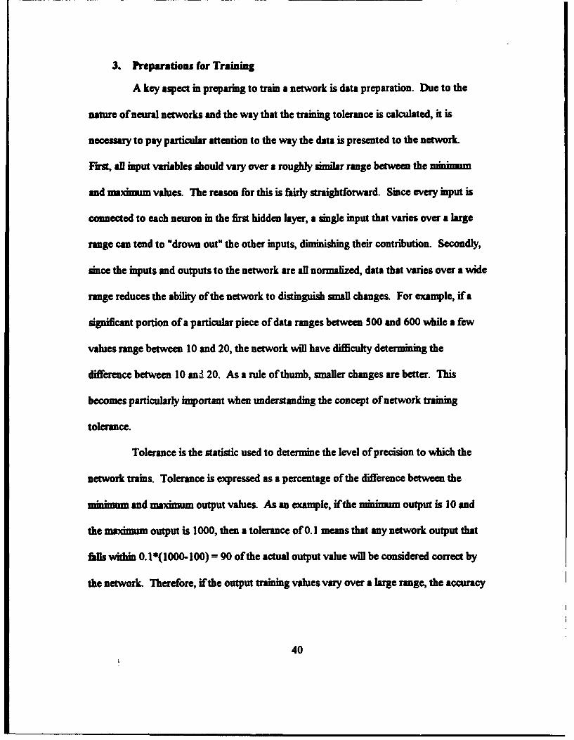
3. Preparations for Training
A key aspect in preparing to train a network is data preparation. Due to the
nature of neural networks and the way that the training tolerance is calculated, it is
necessary to pay particular attention to the way the data is presented to the network.
FMrst, all input variables should vary over a roughly similar range between the minimm
and maximum values. The reason for this is fairly straightforward. Since every input is
connected to each neuron in the first hidden layer, a single input that varies over a large
range can tend to "drown out" the other inputs, diminishing their contribution. Secondly,
since the inputs and outputs to the network are all normalized, data that varies over a wide
range reduces the ability of the network to distinguish small changes. For example, if a
significant portion of a particular piece of data ranges between 500 and 600 while a few
values range between 10 and 20, the network will have difficulty determining the
difference between 10 anl 20. As a rule of thumb, smaller changes are better. This
becomes particularly important when understanding the concept of network training
tolerance.
Tolerance is the statistic used to determine the level of precision to which the
network trains. Tolerance is expressed as a percentage of the difference between the
minimum and maximum output values. As an example, if the mininmum output is 10 and
the maximum output is 1000, then a tolerance of 0.1 means that any network output that
falls within 0.1"(1000-100) =90 of the actual output value will be considered correct by
the network Therefore, if the output training values vary over a large range, the accuracy
40
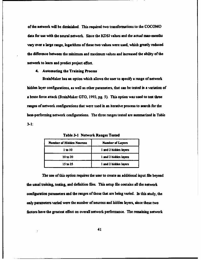
of the network will be diminished. This required two transformations to the COCOMO
data for use with the neural network. Since the KDSI values and the actual man-months
vary ova a large range, logarithls of these two values were used, which greatly reduced
the difference between the minimum and maximum values and increased the ability of the
network to learn and predict project effort.
4. Automating the Training Process
BrainMaker has an option which allows the user to specify a range of network
hidden layer configurations, as well as other parameters, that can be tested in a variation of
a brute force attack (BrainMaker GTO, 1993, pg. 5). This option was used to test three
ranges of network configurations that were used in an iterative process to search for the
best-performing network configurations. The three ranges tested are summarized in Table
3-1:
Table 3-1 Network Ranges Tested
Number of Hidden Neurons Number of Layers
I to 10 1 and 2 hidden layers
10to 20 1 and 2 hidden layers
15 to25 1 and 2 hidden layers
The use of this option requires the user to create an additional input file beyond
the usual training, testing, and definition files. This setup file contains all the network
configpurtion parameters and the ranges of those that are being varied. In this study, the
only parameters varied were the number of neurons and hidden layers, snce these two
factors have the greatest effect on overall network performance. The remaining network
41
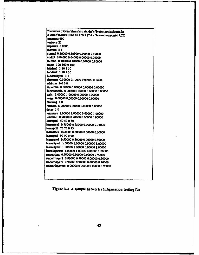
parameters (which deal mostly with the learning rate associated with the Delta rule) were
fixed with the exception of training tolerance, which was allowed to decrease in a stepwise
pattern from 0.1 to a limit of 0.04. The stepwise decreases in tolerance are triggered
when the network learns all the training facts at the current training tolerance. The testing
tolerance was specified as 0.2. An example of the setup file for this option is shown in
Flgu 3-3:
The training and testing data files consisted of the COCOMO data modified as
mentioned previously by changing the KDSI and effort values into logarithmic values.
There were 42 training patterns and 21 testing patterns. The network definition file
consisted of a generic network definition file that provided the ranges of the input values
and the variable names, similar to the file shown in Figure 3-1.
Once the three ranges of configurations had been tested and all of the results
written to three output files, the top performing networks were selected. The selections
were made by reading all of the output flies into Quattro Pro for Windows spreadsheets
and sorting the results based on the number of correct outputs for both the training and
testing data sets. After the sorting process, the networks shown in Table 3-2 were chosen
for fiuther training at a more detailed level The choice of this iterative process was based
upon several factors that mainly involved hardware and software constraints. The
hardware constraint concerned the disk space required to save the testing results. In the
Initial round oftesting, the statistics for the testing data set were written to disk every 25
=s Each of these runs took approximately four to five hours on a 33 MHz 486
42
fllenames c:rainthesiskitrain.de €: ainniheskitrainfctc:birain~dhesis•€ltrain.tst GTO.STA c:Wuain~Wsis'Ls4.ACCmuxnm 400NO= ua25upwM.e 0.2000Current Ustaol 0.10000 0.10000 0.00000 0.10000endtol 0.04000 0.04000 0.00000 0.04000tolmuht 0.80000 0.80000 0.00000 0.80000tolpct 1001000100hiddenl 110 110hiddod 11 0 110biddenlayers 31decreUe 0.100000.100000.000000.10000addruns 0000inputmin 0.00000 0.00000 0.00000 0.0000functiosnin 0.00000 0.00000 0.00000 0.00000pin 1.00000 1.00000 0.00000 1.00000noise 0.00000 0.00000 0.00000 0.00000blurring 10random 5.00000 5.00000 0.00000 5.00000delay 10I'Marate 1.00000 1.00000 0.00000 1.00000learninit 0.90000 0.90000 0.00000 0.90000earnpctl 5050050
limaratel 0.75000 0.75000 0.00000 0.75000learnpct2 75 75 0 75earnrate2 0.60000 0.60000 0.00000 0.60000learnpcO 9090090learnue3 0.50000 0.50000 0.00000 0.50000learwlayerl 1.00000 1.00000 0.00000 1.00000learnayer2 1.00000 1.00000 0.00000 1.00000learnlayerout 1.00000 1.00000 0.00000 1.00000smoothing 0.90000 0.90000 0.00000 0.90000snoothlayerl 0.90000 0.90000 0.00000 0.90000smoothlayer2 0.90000 0.90000 0.00000 0.90000
ay 0.90000 0.90000 0.00000 0.90000
Figure 3-3 A sample network configuration testing file
43
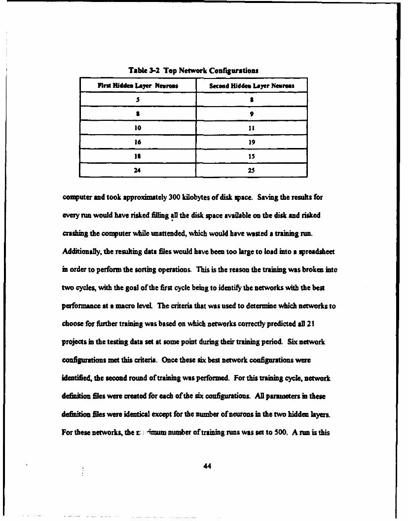
Table 3-2 Top Network Configurations
First Hidden Layer Neurons Second Hidden Layer Neurons
5 1
8 9
10 11
16 19
18 15
24 25
computer and took approxdmately 300 kilobytes of disk space. Saving the results for
every run would have risked filing !al the disk space available on the disk and risked
crashing the computer while unattended, which would have wasted a training run.
Additionally, the resulting data files would have been too large to load into a spreadsheet
in order to perform the sorting operations. This is the reason the training was broken into
two cycles, with the goal ofthe first cycle being to identify the networks with the best
performance at a macro level The criteria that was used to determine which networks to
choose for further training was based on which networks correctly predicted all 21
projects in the testing data set at some point during their training period. Six network
configurations met this criteria. Once these six best network configurations were
identified, the second round of training was performed. For this training cycle, network
definition fWles were created for each of the six configurations All parameters in these
definition files were identical except for the number of neurons in the two hidden layers.
For these networks, the r,. mum number oftraining runs was set to 500. A run is this
44

sense is defined as a pass through the entire training data set in which fitness statistics are
accumulated for the current configuration and weight vector set. The COCOMO training
and testing files wer provided as inputs. Training and testing statistics for all 300 nims
were accumulated in separate files for each of the six configurations. Once this cycle of
tang was over, the testing and training statistics files were again read into Quattro Pro
for Windows spreadsheets and analyzed to determine the optimum number of training runs
for each ofthe six configurations. This optimum point was based on the run waere all 42
projects in the training data were correctly predicted and the network training tolerance
was at a minimum for the training cycle. When this point was determined for each
network, the training process was repeated from the beginning up to this optimum
performance point. The analysis ofneural network performance is based upon the results
obtained from these final versions of the six networks. The definition files for these
networks are shown in Appendix E.
This entire network training process starting with the six network configurations
was repeated a second time in order to test the performance of the neural network on a
data set separate from Boehn's COCOMO data set. In this second round of
experimentation, all of the 63 COCOMO projects were used as the training set, and the 13
projects that make up the Kemmerer data set were used as the testing set.
45

C. GENETIC ALGORITHM PROCEDURES1. Genetk Algorithm Goal
The goal of the second group of experimts in this thesis was to use a genetic
algorithm to determine an optimum set of values for the cost drivers, coefficients, and
exponents for the Intermediate COCOMO model In this group of experiments the inputs
to the genetic algorithm included the Intermediate COCOMO model structure,
MM - Effort Adjustment Factor*COEFF*(Adjusted KDSI)**EXP
and the partitioned COCOMO data with two modifications. The first modification to the
COCOMO training and testing data set prior to using the genetic algorithm consisted of
multiplying the annual adjustment factor and KDSI values together to obtain the adjusted
KDSL This action was taken since the Annual Adjustment Factor provided no additional
information to the genetic algorithm process in the absence of information on how it was
derived. The second modification consisted of expressing the cost drivers by their literal
values, such as HIGH, LOW, or NOMINAL, vice their numeric values.
2. Genetic Algorithm Software
The genetic algorithm software package used was GAucsd 1.4, a C-language
genetic algorithm developed by Nicol Schraudolph of the University of California, San
Diego, based on previous work by John Grefenstette of the Naval Research Laboratory.
The uncompiled C code for GAucsd 1.4 is publicly available via anonymous ftp on the
Internet and can be adapted to any machine that has a C compiler. In this case the target
46

platform was a Sun workstation. The choice of GAucsd 1.4 was based on its availability
and case of use. This package is well-designed in that the user has only to suppl a
chromosome structure and a fitness function (written in C) that defines the problem.
GAucsd 1.4 provides the rest of the finctionality required in a genetic algorithm, such as
population initialization, crossover, and mutation. GAucsd 1.4 also provides an awk
language macro that integrates the user defined fitness function and adds in the code
required to implement the genetic algorithm operations. This design feature relieves the
user f the task of code integration. (Schraudolph and Greffenstette, 1992, pp. 9-12)
3. GAucsd Preparation
Tle chromosome structure defined in the genetic algorithm fitness finction used
in this study consisted of a string of 96 numbers that represented all of the cost driver
values, along with the coefficients and exponents for all three project development modes.
Since there are a maximum of six values for each cost driver and a total of fifteen cost
drivers, the first 90 numbers represented the cost drivers. Although most cost drivers
have less than six values, a total of six values were reserved for each driver. This aided in
the structure of the problem by allowing the indexing process to operate as if the first 90
numbers represented a pseudo 6 x 15 array. The excess cost driver values in no way
impeded the functionality of the genetic algorithm The numeric values derived by the
genetic algorithm were substituted for the literal values in th-e COCOMO training set
which were stored as index values in a C table structure. These first 90 values were
allowed by the fitness function to range from 0.5 to 2.0. The 91st through 93rd numbers
47

represented the coefficients for eta development mode and the 94th through 96th
numbers represented the exponents for each development mode. These last six values
were allowed by the fitness function to range from 0.0 to 4.0. The choice ofthese ranges
was somewhat arbitrary but allowed for a greater range of values than those exprea.d in
Boehuns Intermediate COCOMO model. The actual fitness measure for each member of
the population was initially the average relative error of the actual effort in the COCOMO
training data set versus the estimated effort calculated by the fitness function. This
estimated effort was calculated using the Intermediate COCOMO model as a template.
The genetic algorithm derived numeric values for the literal cost driver values, along with
the coefficient and exponent values appropriate for each project's development mode then
were used as inputs into the Intermediate COCOMO model. The capability to impose
constraints on the values generated by the genetic algorithm was also provided and is
expanded upon later. The GAucsd user-defined fitness function is shown in Appendix F
4. Initial Genetic Algorithm Benchmarking
Along with the user-defined fitness funiction, the other input to the GAucsd 1.4
program is the default file that specifies population size, crossover rate, mutation rate, and
number of generations. The first step in using the genetic algorithm centered on finding an
effective population size and crossover rate to use with the 960 bit chromosome. This
was accomplished by a series of test runs using various population sizes and crossover
rates while keeping mutation rate and number of generations constant. The test runs are
summarized in Table 3-3.
48

Table 3-3 Genetic Algorithm Benchmark Tests
P opulation Sizes Tested 100,200,1000
Crossover RatesTested 0.5,1.5,2.5,3.0,5.0
Mutation Rate 0.00002
Number i f Generations 2,000
The training data for this benchnarking process consisted of the entire
COCOMO project data set. The entire set was used to examine how well the values
derived from the genetic algorithm performed with respect to the values determined by
Boehm bin his original model. The results of this initial round of benchmarking showed
that a population size of 200 and a crossover rate of either 3.0 or 5.0 performed the best
in almost every case. The crossover rate greater than one meant that the chromosome
underwent several crossovers in each generation. A sample of the genetic algorithm
default file is shown in Figure 3-4.
After the optimum population size and crossover rates were determined, nine
versions of the fitness finction were prepared. These versions differed based on how the
fitness of each member of the population was measured and how the previously mentioned
constrints were applied. The three fitness measures used in the experiments were
average relative error, mean error, and mean-squared error and these measures were
calculated as shown in Table 3-4.
49
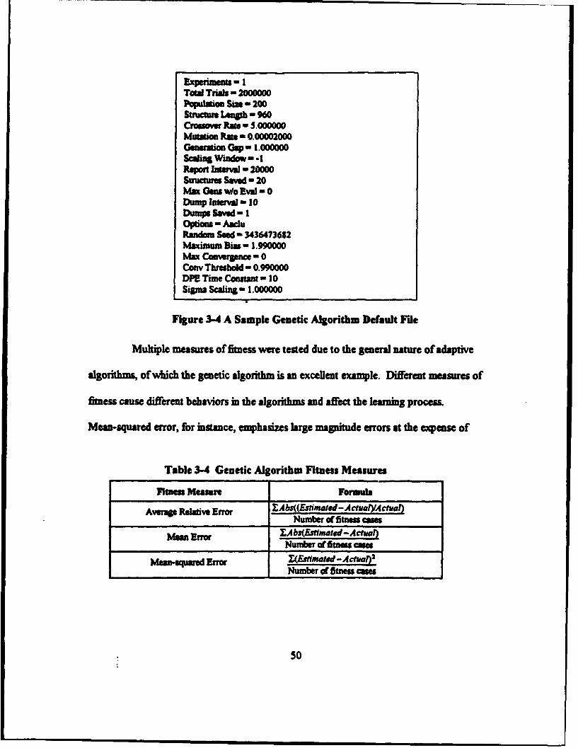
Total Trials - 2000000Populatio Sine- 200Strctur Lmopb - 960Crossover Ras - 5.000000Mutation Rae - 0.00002000GeneMion Gap- 1.000000Scaling Window -=-IRipen Interval - 20000Stuactures Saved - 20Max Gens wo Eval - 0Dump Interval- 10Dump Saved - iOptions - AawuRandom Seed - 3436473682Maximum Bias - 1.990000Max convergenc-=0Cony Threshold - 0.990000DPE Time Constant - 10Sigrna ScalingL- .0000o
Figure 3-4 A Sample Genetic Algorithm Default Fide
Multiple measures of fitness were tested due to the general nature of adaptive
algorithms, of which the genetic algorithm is an excellent example. Different meaures of
fitness cause different behaviors in the algorithms and affect the learning process,
Mean-squared error, for instance, emphasizes large magnitude errors at the expense of
Table 3-4 Genetic Algorithm Fitness Measures
itness Measure Formula
Averag Reativ Error E:Abs((EstmaIed-Actuat)/AetyI)__________________ Number of fitness ue
Number of Bums camett~ E~Of ZAbs(Efimaled-AchuaI__Mean___Error__ Numnber of flists can
Mensur ro £(Ef~timated-Aceal) 2
Number of fitness cases
so
smaller magnitude errors This type of behavior caused the genetic algorithm to focus on
learning the larger software projects that had lrge errors at the expense of the smller
projects This behavior led to poor results. Mean error reduced this tendency to a degree,
but the best learning performance was found when using average relative error. In these
experiments, this fitness measure equalized the effort the genetic algorithm expended
learning all of the projects since error was expressed as the average percentage difference
between the estimated value and the actual value. A secondary observed benefit of this
measure was that both mean error and mean-squared error were also minimized when
using this fitness measure even though neither of these fitness measures were explicitly
expressed in the fitness function.
5. Genetic Algorithm Constraints
The final aspect of the various fitness functions involved the imposition of
various degrees of constraints on the values generated by the genetic algorithm. An
inspection of Boehm's COCOMO cost driver, coefficient, and exponen values reveals
certain patterns or constraints. For example, in the case of the COCOMO exponents, the
magnitude of the exponent increases as the mode shifts from organic to semidetached to
embedded. Conversely, the coefficient decreases as the same mode shifts occur. Similar
patterns can be seen in the values ofthe cost drivers. When inspecting the cost driver
table, the magnitude of the first seven cost drivers increases when moving from a value of
Very Low to a value of Extra High. The opposite movement occurs in drivers eight
through fourteen. In this case the magnitude of the driver decreases as the value shifts
: 51

from Very Low to Very High. The value of the final cost driver, required development
schedule (SCED), moves in a high-low-high manner as the value shifts from Very Low to
Very High. These patterns can be interpreted as constraints that the cost driver values
should obey. To teog whether or not these constraints added to the ability of the genetic
algorithm to lam the project data and find an optimal set of values, these constraints were
embedded in three versions of the fitness function. In the first version, no constraints were
placed on the order of the cost drivers, exponents, or coefficients. In the second version,
penalty measures were introduced on the cost drivers so that if the previously identified
patterns in the first 14 cost drivers (SCED was allowed to vary without constraint) did not
appear in the chromosome, the fitness of the individual was penalized based upon the
degree of non-compliance. In the final version of the constrained fitness function, penalty
measures were introduced on the generation of the exponents and coefficients as well as
the cost drivers.
6. The Genetic Algorithm Testing Process
The nine fitness functions used for training the genetic algorithm were
constructed using the three me.sures of fitness and the three constraint levels previously
described. Testing was performed using a population size of 200 and crossover rates of
3.0 and 5.0 with the number of generations set at 5000 for all tests. There were 18 total
tests and each test took approximately two to four hours on a Sun workstation. The top
twenty chromosomes in each test were saved to an output file and read into a Quattro Pro
for Windows spreadsheet. The chromosome values wih the best fimess in each run were
52

translated into their associated COCOMO model values using a previously constructed
secres of linked spreadsheets. This table oftranslated COCOMO model values was then
linked to the tent data set in such a manner as to allow for automatic updating of the teat
data and its associated performance measures whenever new chromosome data was pasted
into the spreadsheet. The results of all 18 tests were processed in the same manner.
A slightly different procedure to that previously described was used when the
genetic algorithm was trained using all 63 COCOMO projects and tested with the
Kemmerer project data. In this case, the best parameter set from the original genetic
algorithm benchmarking tests was used along with the full range of constraints in the
fitness function. The use of all of the constraints was based upon the results observed in
the first phase of testing. The number of generations was increased from the
benchmarking level of 2000 to 5000. The top twenty chromosomes from this run were
again saved to an output file that was loaded into a spreadsheet holding the Kemmerer
data. The performance of the genetic algorithm with respect to the Kemmerer project set
was then calculated.
D. GENETIC PROGRAMMING PROCEDURES1. Genetic Programming Software
The goal of the final group of experiments in this thesis was to test the ability of
genetic programming to derive an explicit cost estimation model given only the COCOMO
data and a fitness function. The genetic programming software used was SGPC: Simple
Genetic Programming in C by Walter Alden Tackett and Aviram Carma This software
53
is basd on the original LISP code published by Koza in his book and is available via
anonymous ftp from the Santa Fe Institute and the University of Texa This software
provides all the functionality required to apply genetic programming to a variety of
problem domains The genetic operations of population initialization, crossover,
reproduction, and mutation are fully supported by this software. The usa is only
responsdble for defining functions specific to the problem at hand, ensuring closure of the
flnctions, and providing the appropriate fitness function and terminal set. T1his software
also has the capability to train and test simultaneously, which reduces the
post-experimental processing of the output expressionL Due to the memory requirements
and CPU intensive nature of this application, the target platform for this application was a
Sun workstation.
2. Genetic Programming Preparation
Preparation for the genetic programming process using the SGPC software
involved five steps. In the first step the fimctions available for use in the S-expressions
were defined. Since this set of experiments was basically a problem of regression, the
standard mathematical operations of addition, subtraction, multiplication, protected
division, and exponentistion were defined as operators in SGPC. The protected division
operator is a specially defined division operator that provides closure for the case of
division by zero. When this event occurs, the operator is defined to return a value of one.
In the second step the C-language program structure that provides the terminal
set (variable declarations) and the training data was constructed. This procedure was
54

performed using a script written in perl that took the tab-delimited ASCII file containing
the COCOMO training data and built a C source code file. This C source code file made
the variable declarations that defined the terminal set and created the table structure
cotai training data. The training data for this set of expeiments consisted of the
sae projects as those used for the previous experiments. The first round of experimints
used the same 42 COCOMO training projects and 21 COCOMO testing projects. 1n the
second round of experiments the entire 63 project COCOMO project set was used for
training while the 15 project Kemmerer data set was used as the testing data. The training
data input variables were KDSI, the annual adjustment factor, and the fifteen cost drivems
The actual effort associated with each project was the dependent variable. The project
mode was not included in the training set since mode is a fixed descriptor of project
classification and not a variable. Consideration was given to partitioning the data by mode
but this idea was discarded, since the resulting training and testing bets would be so small
no conclusions could reasonably be drawn from the result
The third step in the genetic programming preparation process was the definition
of the fitness measure embedded in the "flzness.c" source code file. With the Imowledge
gained from the sequence of genetic algorithm experiments, the fitness measure for the
genetic programming sequence was b-sed on average rekaive error. The use of average
relative error is also supported by the fact that some initial genetic programming test rims
performed using the COCOMO data with a different fitness measure, mean-squared error,
showed very poor performance.
55
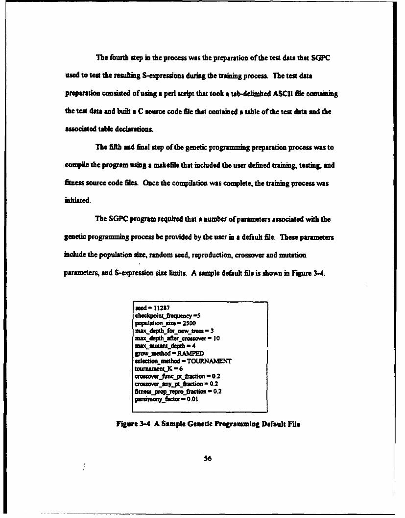
The fourth step in the process was the preparation of the test data that SGPC
used to tea the resulting S-expressions during the training proces. The test data
preparation consisted of umg a perl script that took a tab-delimited ASCII file comaining
the test data and built a C source code file that contained a table of the test data and the
associated table declarations.
The fifth and final step of the genetic programming preparation process was to
compile the program usgng a makefile that included the user defined training, testing, and
fitess source code fileL Once the compilation was complete, the training process was
initiated.
The SGPC program required that a number of parameters associated with the
genetic programming process be provided by the user in a default file. These parameters
include the population size, random seed, reproduction, crossover and mutation
parameters, and S-expression size limits. A sample default file is shown in Figure 3-4.
seed- 11287checkpoinftfequency -5populaion size - 2500maxdepth fornew trees -3max._deph..aftercroswver = 10max mnutant depth - 4pow method - RAMPEDselctionumethod - TOURNAMENTtournamientK -6crasmaerncptfaci6o - 0.2crouoeruiy.. ofrn-tio - 0.2fitnesjrop repro hctiion - 0.2parsimo�3 r = o0.01
Figure 3-4 A Sample Genetic Programming Default File
56
A population size of 2500 was used for all the genetic programming experiments
in this study. Cboice ofthis population size was basically a compromise between the need
to provide a large population to ensure genetic diversity and the memory available on the
Sun workstation. It is important to remember that during portions of the genetic
programming process, two copies of the entire population are stored in memory. If these
populations begin to contain large S-expressions, the memory requirements can be huge,
easily exceeding 50 or 60 megabytes. Tournament selection was used to select
S-expressions for the reproduction process with a tournament size of six. The parsimony
factor included in the default file is an SGPC variable that can be used to reward
S-expressions for size of structure as well as performance, with smaller structures being
viewed as better than larger ones when performance is equivalent. While the use of
parsimony is optional in genetic programming, it was used in the COCOMO runs at
various settings The crossover and S-expression size parameters were also varied so that
a total of seven runs using the COCOMO training and testing data and seven runs using
the COCOMO and Kemmerer data were completed. The results of each rim, which
contained the best structure for each generation and its associated fitness, were written to
an output file.
Once the testing process was completed the output files were processed by first
fruning an Ami Pro macro on the output file. This macro substituted the Quattro Pro
spreadsheet coordinates for each ofthe input variable names. Using this procedure
allowed the best structure from each output file to be pasted directly into a spreadsheet
57

cl, whore the performance calculations were made automatically using a set of linked
preadshedta This action greatly reduced the processing time required for each output
f8.
58
IV. ANALYSIS OF RESULTS
A. MEASURES OF PERFORMANCE
The results ofthe experiments for all three machine learning techniques were analyzed
in the same manner to determine each techique's performance. Three measures of
performance were used for all ofthe techniques. These three measures consisted of the
average magnitude of the relative error, the standard deviation of the magnitude of the
relative error, and the regression coefficient, f-squared, of the estimated man-months
versus the actual man-months. The choice of these three performance measures was based
upon the work done by Kemnmerer (1987), in which he analyzed the performance of
several popular software cost estimation models using a 15 project data set that he
developed. These are the same 15 projects that were used as one of the sets of testing
data in this study. The use of the magnitude of the relative error is intended to measure
the accuracy of each model The closer this measure is to zero, the greater is the accuracy
of the model. The f-squared measure gives the correlation between the estimates of each
model and the actual project results. A perfect correlation gives an R-squared value of
one. This measure is meant to act as a sort of *reality check" on the models' outputs in
seeing whether the project estimates track in a predictable manner with the project actuals.
Since each machine learning experimental procedure involved two phases
corresponding to trY, different software development domains, the measures of
perfonmance are able to provide insight in two distinct manners. In the first phase of each
59
experimental procedure, COCOMO data was used for both training and testing. The
performance measures for each of the methods during this phase gives insight into which
of the machine enermaed models perform beat when operating in a specified development
domain. Where appropriate, comparisons with the estimates provided by Intermediate
COCOMO are made. In the second phase of each experimental procedure, the sau
testing data set Kemmerer (1987) used when he made his study of several popular models
was used as the testing data set for the machine generated models. In this phase, it is
possible to compare the estimating capabilities of the models developed by the three
machine-learning techniques with several well-known cost-estimation models by using the
results Kemmerer obtained in his study. These models include SLIM, ESTIMACS,
Function Points, and COCOMO. This comparison is useful because it gives an indication
of the ability of the machine generated models to generalize across development domains,
which is critical for a model, or modeling technique, to be successful
The machine generated models were also analyzed to see if their structure could
provide insight into the general relationships between the input variables and the model
outputs. This analysis was performed to see if the machine generated models detected any
relationships among the variables that may have gone unnoticed.
B NEURAL NETWORKS1. First Phase Results
The initial phase ofneural network training involved the use of the COCOMO
data set for both training and testing. Six networks were trained using 42 projects from
60

the COCOMO da& set. Testing was conducted using the remaining 21 projects. Table
4-1 dMows the performance statistics based on the results of these tests for the six best
Table 4-1 Neural Net Performance Results
COCOMO Training and Testing Data
Network Coefiguratif Ag RIel Err Std Dev Err R-qWared
M)(_ (_. _ _ 40
3/3 91.89 ".17 0.755
8/9 89.40 6.26 0.707
11/10 105.96 126.06 0.816
16/19 68.10 68.61 0.726
3/IS -136.84 272.68 0.753
24/25 110.17 109.93 0.705
mnt COCOMO 16.33 15.76 0.91
XX/XX - Hidden Layer I/Hidden L 2
20 Input Neurons - I Output Neuron
As Table 4-1 indicates, neural networks are not highly accurate in their
estimates, but their estimates do correlate relatively good to the actual project efforts.
Results of this type are consistent with the typical expectations of a neura network. The
strength of neural networks lies in their ability to provide generalized outputs eased on
their inputs From this perspective, the neural Llwork results from the first phase of the
exprment are positive. The most accurate neural network with 16 neurons in the first
hidden layer and 19 neurons in the second hidden layer, is capable of'providin$ a general
61
idea of the mapitude of the effort required for a particular project being developed within
the same domain in which the network was trained. The correlation coefficient,
R-squared, of 0.726 indicates that this estimate has a fairly strong relationship with the
actual project effort. Why this particular network performs better than the others is not
explicitly determinable. In general, a network is successful when it has just enough
neuons to provide a capability for feature detection, but not so many neurons that it just
"memorizes" the training cata. While not as accurate as the algorithmic model,
Intermediate COCOMO, a network has the advantage of requiring less analytical skill to
develop and use, and it probably requires less development time. Based on the
performance characteristics as observed in Table 4-1, the best use of a neural network
would probably be at the early stage ofproject development, where a manager could
perform "what-ifr analyses using various input combinations and obtain results very
quickly with a minimum of setup. Additionally, by continually retraining the model with
new projects the manager could gain fu•ther advantages since the network model would
be continual•y calibrating itselfthrough this retraining process. If'the organization also
uses an algorithmic model for cost estimation, and correlates its estimates with those of
the neural network, a sort of early warning system" that could indicate when recalibration
of the algorithmic model is required could be established. A significant drop in the
correlation between the two estimation methods could be an indicator that the algorithmic
model is in need of calibration.
62

The most interesting aspect of this phase of experimentation is the effect
network configuration has on performance. While the accuracy of the estimate varies over
a range of approximately 70 percent, the standard deviation varies ova a range of
approximately 200 percent. These results indicate that when preparing to use a neural
network a good strategy would be to begin with several candidate configurations and
continue to maintain and compare them until a statistically sound analysis can be
performed to determine the best configuration. As for finding the best configuration, the
BrainMaker (1992) thumb rule of using the number of inputs and outputs divided by two
or the Eberhart and Dobbins (1990) rule of using the squame root of the sum of the inputs
and outputs plus a couple would have both provided networks close to the ones found
using the brute force search. However, with the power available in current personal
computers the BrainMaker brute force search is not an unreasonable or even overly
time-consuming approach to take initially.
2. Second Phase Results
In this phase of the neural network experimentation process the entire 63 project
COCOMO data set was used for training and the 15 project Kemmerer data set was used
for testing. As previously stated, the network configurations from the first phase were
retrained to the optimal performance point for the 63 training projects and then tested.
The results of this phase of tests are shown in Table 4-2.
The second phase results using the Kemmerer testing are very interesting. As
can be seen from Table 4-2, the top performing neural networks are competitive with, and
63
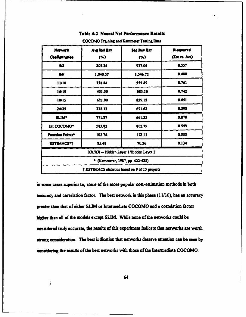
Table 4.2 Neural Net Performance Results
COCOMO Trang anod Kemnerem Testin Doa
Netmek Av Rd Err SBd DV I' 3-equared
C..Amfut (%) (%) (Eat v. Act)
5/8 803.24 937.05 0.557
8&9 1,040.57 1,546.72 0.438
11/10 328.54 555.49 0.761
W19 451.30 633.10 0.742
18/15 621.00 829.12 0.651
24/25 338.12 691.62 0.591
SLIM* 771.87 661.33 0.878
IN COCOMO) 583.82 862.79 0.599
Function Pointso 102.74 112.11 0.553
ESIMACSt 8.5.48 70.36 0.134
XJ/XX - Hidden Layer 1/Hidden Layer 2
"0 (Kemmerer, 1987, pp. 422-425)
t ESTNAACS stistics based on 9 of 15 projects
in some cases superior to, some of the more popular cost-estimation methods in both
accuracy and correlation fictor. The best network in this phase (11/10), has an accuracy
greater than that of either SLIM or Intennediate COCOMO and a correlation factor
higher than all of the models except SLIM. While none of the networks could be
considered truly accurate, the results of this experiment indicate that networks are worth
strong consideration. The best indication that networks deserve attention can be sen by
considering the results of the best networks with those of the Intermediate COCOMO.
64

Both the networks and Intermediate COCOMO are based on the same 63 project data set,
yet the best networks pe•fon sgnificantly better. These results seem to indicate that the
top networks are capable of capturing some level of mets-knowledge about the
relationships between the cost-estimation inputs and the output.
With the relatively small amount of data in both number of inputs and projects
that was used for training these networks, the level ofperformance obtained is still
significant. However, the sensitivity to configuration is once again apparent. Al six
networks "learned" the 63 projects in the COCOMO data set but their performance on the
Kenmerer data ranges greatly in both accuracy and correlation. This divergence in the
range of performance results appeaps to to magnified by the change of development
domaim This reinforces the suggestion that managers should initially maintain multiple
network configurations until some level of confidence is obtained as to which network is
truly the top pf.former.
3. Neural Network Structural Analysis
Although neural networks are relatively easy to construct and operate, it is
difficult to explicitly analyze bow they are processing their inputs. One method, suggested
by a BrainMaker user and posted on Compuserve, can at least provide the user with
insight into which inputs affect the behavior of the network the greatest. In this method
the first step is to extract the complete set of connection weights from the BrainMaker
network defition file anJ strip the bias weights off of each layer. The second step is to
take the absolute value of all the weights. And finally, in the third step, a series of matrix
65
inhiplicaticms are perfomed, begining with multiplying the output layer connection
weights by the connection weights to the second hidden layer. This process is repeated in
a stepwise manner backward through afl ofthe hidden layers until a single weight vector
remains This resulting weight vector shows the magnitude ofthe connection wights that
each input 'sees through the network. Examining this vector can give some indication of
which inputs are affecting the network output to the greatest extent. Unfortunately, these
results do not indicate whether these weights affect the output positively or negatively
since only the magnitudes are used. Still, this approach is usefu because the usae can at
least see what inputs the network considers important. This matrix multiplication analysis
was conducted on three of the networks derived in the second phase of the neural network
experiments, Two ofthe top networks, 11/10 and 16/19, along with the worst network,
8/9, were examined using this method. The top 10 connection weight magnitudes for the
input neurons in these three networks are shown in Table 4-3.
"The results shown in Table 4-3 provide some interesting insights into how each
of these networks are manipulating the inputs to the network in order to obtain the effort
estimate. For example, the two best networks deemphasize the effect the size of the
project has on the effort estimate while the worst network views size as having the top
effect an the output. The comparison ofhow these networks view project size
eacapsulates the argument made by various researchers that "lines of source code is in
actuality a poor predictor ofproject effort (Kemmerer, 1987, pg. 418). One factor that all
of the networks examined do have in common though is their emphasis on project
66

Table 4-3 Top Network-Influencing Input Neurons
Newrk I1/10 Network 16119 Network M/
hVA _ _ __t bhpa~UW W MMaW
TURN 266.28 PCAP 462.70 LOGKDSI 242.06
ClX 208.23 TURN 47.40 SD 238.54
AMXP 181.72 STOR 436.58 TURN 205.07
PCAP 168.38 SD 398.55 PCAP 192.67
ORG 166.97 CPLX 388.80 AEXP 179.77
TnIE 163.14 LOGKDSI 371.82 E 175.35
ACAP 159.61 TIME 366.50 ORG 169.01
VIRT 157.12 AEXP 363.64 CPLX 164.78
LOGKDS! 149.15 ORG 363.12 VIRT 158.63
VEXP 148.42 TOOL 345.72 SCED 141.67
complexity, computer turnaround time, and programmer capability. This emphasis on
project complexity and programmer capability is also apparent in the cost driver values
that Boehm assigns to these values but the emphasis that the networks place on computer
turnaround time is not reflected in the values that Boehm assigns to this driver (Boehm,
1981, pg. 118). Looking at these results from the other direction, the emphasis that
Boehm places on the capability of the analyst is not reflected in the analysis of the
networks. This driver only appears once in Table 4-3, and is ranked only seventh.
While not conclusive by any measure, this type of analysis can provide a project
manager some insight into which network inputs are affecting the output to the greatest
67
degree and can setve as a type of sensitivity analysis that can provide indications of areas
that may possibly require a higher level of attention.
C. GENETIC ALGOiT HMS1. First Phase Results
The first phase of the genetic algorithm experiments used the COCOMO
training and testing data sets and Intermediate COCOMO as a model template. In this
phase 18 different fitness functions were tested. These fitness functions differed based on
the aossover rate, the measure by which the error was determined, and the degree to
which the constraints on the values generated by the genetic algorithm were applied.
Table 4-4 provides a summary of all of the tests conducted.
As previously mentioned, different fitness measures were tested in order to see
which fitness measure most effectively forced the genetic algorithm to find the optimal
values of the cost drivers, coefficients, and exponents. The constraints invoked during the
various tests reflected the patterns meted in Boehm's values for the cost drivers. The "no
constraints' tests meant that all values were free to seek optimal values independent of
each other. The "cost drivers only" constraint penalized the fitness of the genetic
algorithm proportionate to the degree to which the results failed to match the patterns
noted in Boem's cost driver tables. The "All constraints" constraint extended the "cost
drivers only" penalties to the patterns observed in the coefficients and exponents. A
graphical representation ofthe results of all of these experiments is shown in Figure 4-1.
68

Table 4-4 Genetic Algorithm Test Series Summary
Test Number ri5amss Measure Censtraints Crosver Rate
I AvgR Error None 3.0
2 Avg Rul Error None 5.0
3 Avg Re Error CAst Driven 3.0
Onl
4 Avg Rd Error Cost Drivers 5.0
_nly
S Avg Rel Error AI Constraints 3.0
6 Avg Rel Error All Constraints 5.0
7 Mean Error None 3.0
8 Mean Error None 5.0
9 Mean Error Cost Drivers 3.0
Only
10 Mean Error Cost Drivers 5.0
Only
S1 Mean Error All Constraints 3.0
12 Mean Error All Constraints 5.0
13 Mean Squared Err None 3.0
14 Mean Squared Err None 5.0
15 Mean Squared Err Cost Driven 3.0
Only
16 Mean Squared Err Cost Driver 5.0
Only
17 Mean Squared Err All Constraints 3.0
18 Mean Squared Err All Constraints 5.0
69
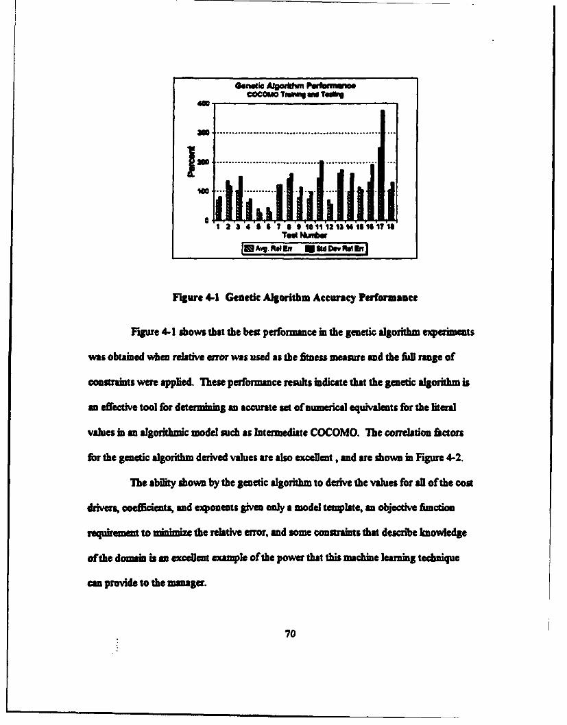
Genieic Aigodmhm PerfwmWw.cocoMo Tnoo"g vn TeGOOg
4U0
m
IN--ISO'1) ... °' .... .. . . .°° - ° ° ° 0 ° ° ° °°
I a 3 4 6 S 7 II 9 101112 14114 1617 isTest Nu~ber
EAvg. R•eIn *UdON ,,I
Figure 4-1 Genetic Algorithm Accuracy Performance
Figure 4-1 shows that the best performance in the genetic algorithm experiments
was obtained when relative error was used as the fitness measure and the fuil range of
constraints were applied. These performance results indicate that the genetic algorithm is
an effective tool for determining an accurate set ofnumerical equivalents for the literal
values in an algorithmic model such as Intermediate COCOMO. The correlation factors
for the genetic algorithm derived values are also excellent , and are shown in Figure 4-2.
The ability shown by the genetic algorithm to derive the values for all of the cost
drivers, coefficients, and exponents given only a model template, an objective finiction
requiremet to minimize the relative error, and some onstraints that describe knowledge
of'the domain is an excellent example of the power that this machine learning technique
an provide to the manager.
70

.mlsf o U A W 0.UMIS
0.2
oi - S1 2 3 4 6 6 7 9 10 11 121U314 151617 16
T"s I~NberW
Figure 4-2 Genetic Algorithm Correlation Performance
Boehm (198 1, pg. 324) describes situations m~ere it is desirable for COCOMO
to be tailored to a particular instalation. Thet procedure outlined for calibrating the model
requires solving a system of linear equations. This, is time-consming, tedious work and it
also fis to take advantage of any domain knowftilge that may have been accumulated by
the organization. The genetic algorithm provides an alternative method to this approach
that is earner, more extensible, and takes advantage of any domain knowledge that the user
wishes to embed in the fitness humction. For instance, assuming a COCOMO template, in
that the effort required is a flaiction of a particular cost driver set, the project size, and a
particular development mode, a user could easily build a new pseudo-COCOMO model
71

that makes use of ny number of cost drivers and modes that the user speciies in the
finess fuction and chromosome structure. Additionall,, the user has the opportunity to
uild into the fitness function amy identified domain knowledge about the reationships that
ave applicable.
I Second Phase Results
in the second phase of the genetic algorithm experzmntatio process the entire
COCOMO data set was used for training and the Kemmee data set was used for testing.
The fitness function for this phase ased the magnitude of the relative error and the fWll set
of consraints, taking advantage of the knowledge pined previously. The results of this
experiment are shown in Table 4-4.
Table 4-4 Phase 2 Genetic Algorithm Performance
COCOMO Training and Kemmerer Testing Data
Model Avg. Rel. Error Std. Dev. Error R-squared
1 (%) (%)
GA Int. COCOMO 831.01 1,363.18 0.472
GA Basic COCOMO 95.34 111.75 0.578
Basic COCOMO) 630.09 684.55 0.680
Int. COCOMOO 583.82 862.79 0.599
SLIM* 771.7 661.33 0.878
Function Points* 102.74 112.11 0.553
ESTAAiACS 1t 85.48 70.36 0.134
(Kemnerer, 1987, pp. 422-425
t ESTIMACS uzuistics bses an 9 of 15 projects
"72
The performance of the genetic algorithm-derived values for the cost drivers
fared poorly when estimating the effort required for the Kemmera projects in fact, the
correlation coefficient for the Intermediate COCOMO model derived by the genetic
algorthm W s lowa for the Keumern data set than the corelation coefficient between the
KDSI and the actual project man-months for this data set (0.47 vs 0.53), indicating that in
this case the Intermediate COCOMO model adds little value. The interesting results in
this experiment are obtained by using the Basic COCOMO model which include: just the
coefficients and exponents and uses no cost driver values The estimates obtained when
using the genetic algorithm derived values for the coefficients and exponents actually give
some of the best results of any model The strongest conclusion that can be made from
these results is that the cost driver values derived by the genetic algorithm are highly
sensitive to the domain in which the model was trained. These results have both positive
and negative impacts. On the positive side, they reinforce the conclusion from the first
phase of genetic algorithm experiments that the genetic algorithm is highly effective at
learning a specific software development domain. On the negative side, they indicate that
any resulting model is likely to be of litte benefit if there is a dramatic shift in the
underlying factors in the development environment.
3. Genetic Algorithm Structural Analysis
The surprising accuracy of the Basic COCOMO model as derived by the genetic
algorithm is the most interesting result of this experiment. A possible conclusion that can
be drawn from this result is that the genetic algorithm has observed a different relationship
73

between the coefficits and exponmts of the COCOMO model than that observed by
Boehm. Table 4-5 dsows the genetic algorithm coefficients and exponent values
compared to those developed by Boehm.
Table 4-5 Comparison of Coefficients and Exponents
Genet* Algorithm Values v. Boebm Vahles
Emeddid Sendmdedw Or
GA Coefficien- 0.429 0.552 2.25
GA Exponents 1.27 1.21 0.510
Doehm Coefficienu 2.8 3.0 3.2
Doehm ExpOneM 1.20 1.12 1.05
(B"ehm, 1981.P& 117)
This comparison between the genetic algorithm derived values and Boehm's
values for the coefficients and exponents indicates that the genetic algorithm detects a
greater diseconomy of scale (exponent greater than one) for both the embedded and
semidetached modes than Boehm does. Also, the genetic algorithm gives a much greate
economy of scale (exponent less than one) to the organic mode than Boehm does. The
diffeenmce in coefficients between the genetic algorithm and Boehm is probably
attributable to the difference in size of the typical projects that are developed in each
mode. The large difference seen in the embedded and semidetached coefficients between
the two vrsions is more than likely a reflection of the genetic algorithm's detection of a
74
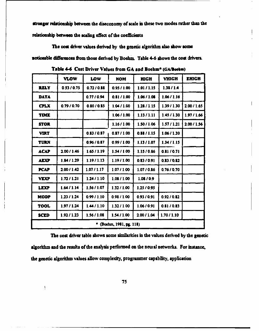
Sr'onger relationship between the diseconomy of sale in these two modes rather than the
relationship between the scaling effect of the coefficients
The cost driver values derived by the genetic algorithm also show some
Noticeable differences from those derived by Boehm. Table 4-6 shows the cost drivers
Table 4-6 Cost Driver Values from GA and Boehm* (GA/Beebn)
VLOW LOW NOM HIGH VICGH V.l11GH
RELY 053 /0.75 0.72/0.18 0.9511.00 1.01/1.15 1.31/1.4
DATA 0.77/0.94 0.81/1.00 1.06/1.08 1.06/1.16
CPLX 0.7910.70 0,8010.85 1.04/1.00 1.21/1.15 1.39/1.30 2.00/1.65
TIME 1.06/1.00 1.13/1.11 1.45/1.30 1.97/1.66
STOR 1.1611.00 1.50/1.06 1.57/1.21 2.00/1.56
VIRT 0.83/0.87 0.87/1.00 0.18/1.15 1.06/1.30
TURN 0.96/0.17 0.99/1.00 1.13/1.07 1.34/1.15
ACAP 2.00/1.46 1.65/1.19 1.54/1.00 1.15/0.16 0.11/0.71
AEXP 1.$4/1.29 1.19/1.13 1.19/1.00 0.83/0.91 0.83/0.12
PCAP 2.00/1.42 1.07/1.17 1.07/1.00 1.07/0.86 0.76/0.70
VrXP 1.72/1.21 1.24/1.10 1.081/1.00 1.01/0.9
LEXP 1.64/1 .14 1.56/1.07 1.32/1.00 1.25/0.95
MODP 1.23/1.24 0.99/1.10 0.981/1.00 0.93/0.91 0.92/0.82
TOOL 1.97/1.24 1.44/ 1.10 1.32/1.00 1.06/0.91 0.81/0.33
SCED 1.92/1.23 1.56/1.08 1.54/1.00 2.00/1.04 1.70/1.10
(Boehm, 1981, 1. 118)
The cost driver table shows some similarities in the values derived by the genetic
algorithm and the results of the anslyis performed on the neural networks. For instance,
the genetic algorithm values allow complexity, programmer capability, application
75
experience, and computer turnaround time to exert a greater variation on the effort
adjument factor than Boehm's values. These are also factors that the top neural
networks emphasized. This cncurence of emphasis between two very differet machine
learning paradigmns may be an indication that greater attention should be paid by managers
to then areas.
D. GENETIC PROGRAMMINGL. F'wst Phase Results
"7he first phase of the genetic programming experimeats used the COCOMO
training and testing data sets. Several runs using the genetic programming software were
made using various default values of such factors as, the maximum depth for new trees,
the maximum depth after crossover, the crossover factors, and parsimony. The parsimony
factor was tried at various levels to see what effect it had on both S-expression length and
generalization characteristics of the resulting expressions. The population size was 2500
for all nis, and the total number of generations for each run was 50. For each run, the
fittest structure from each generation was saved to an outfile file. The fitness measure
used in these experiments was the average magnitude of the relative error. The fitness of
both the training and testing data sets were computed each generation.
The results of this phase of experiments were very encouraging and followed a
distinctive pattern. Initially, the best of generation fitness for both the testing and training
data were roughly of the same magnitude. As each run progressed, the average relative
error for both the testing and training data tended to decline until a point was reached
76

where a divergence was noticed. At this point, the average relative error of the training
data continued to decline while the average relative error of the testing data would begin
to climb, sometimes in a dramatic manner. It was very apparent from this pattern that the
capability of genetic programming to provide a generalized expression is reduced as it
learns the training data to a greater and greater degree. This behavior is especially
noticeable in the second phase of the genetic programming experience when the
COCOMO and Kemmerer data are used.
As for performance, in every run genetic programming was able to learn an
expression for the estimated effort that was both accurate and well-correlated. A
summary of some of the top performers for the frst phase is shown in Table 4-7.
Table 4-7 Genetic Programming Results-Phase One
COCOMO Training and Testing Data
Test i Test 3 Test 4 Test 5 Test 6 Jnt COCOMO
Avgr el Err 39.89 41.9 42.37 42.1 45.32 16.33
Std Dev Err 36.5 39.73 41.06 33.44 40.26 15.76
R-Squared 0.909 0.81 0.71 0.95 0.69 0.991
As Table 4-7 indicates, the accuracy and correlation of the genetic programming
derived expressions are worthy of strong consideration by any software manag,- The
only major hindrance to the easy acceptance of genetic programming as a useful technique
comes from examining the expressions that the genetic program generates. These
expressions can be both intriguing and intimidating to the uninformed user. It is important
77

to remember when usng genetic programming that the genetic program does not have the
domain kmowledge nor the prejudices of the user. This means that the genetic program is
free to use the terminals and finctions provided by the usa in any way that the genetic
program perceives as *fit*. As an example, Figure 4-3 shows one of the expressions
generated by the genetic program during this phase of the experiments.
MM EST - ((((MC)DPO KDSI) + ((TIDE A CPLX) * (KDSI - LEXP ))) AVtrT)
^ACAP) + (((ACAP*((STORP'CPLX)oRELY)) + (((ACAPO(PCAP- ("Ia* ((KDSI
/(((((PCAP*(KDSI AgSOR))4(DATA+((KDSI "SCED). SCED))) AVIRT) *((DATA+ (KDSI
SCED )) +CDSI)) +ACAP)) +(KDSI ASTOR))))) + ((( KDS] * VEXP )r TIMrVEXP)) -
Figure 4-3 A Sample Genetic Programming Expression
As can be seen from Figure 4-3, the expressions generated by the genetic
program can be complex and somewhat cryptic, but they are also accurate. The
expression shown in Figure 4-3 is the expression used to obtain the Test I results shown
in Table 4-7. As Table 4-7 shows, this expression has an average relative eror of
approximately 40 percent and an R-squared value of 0.9.
2. Second Phase Results
The second phase of the genetic pro aimming experiments used the COCOMO
data for training and the Kammerer data for testing. The same variations in program
parameters such as mxinmum tree depth, crossover rates, parsimony, etc., were used in
this phase as in the first phase. The same pattern in the fitness measures for both the
78

traiing and testing data were also observed but in a much more pronounced manner. In
fact, the divergence in fitness between the training and the testing data was so pronounced
that the maxdmm number of generations was reduced from 50 to 20 for this phase of
aperments, A summary of some of the top runs for this phase of experiments is shown
in Table 4-3. The results from Kemmere's analysis are included for comparison.
Table 4-8 Genetic Programming Performance Results
COCOMO Training and Kemmewer Testing Dat
Test Avg Rel Err Std Dev Err R-squamred
(%) (%) (Et vs. Act)
Test 2 109.52 125.85 0.78
Test 3 130.Y7 142.35 0.62
Test 4 59.15 69.5 0.93
Tet 9(a) 112.01 132.15 0.90
Test 9(b) 144.24 167.9 0.83
SLUM 771.87 661.33 0.178
lnt COCOMO" 513.82 862.79 0.599
Function Points* 102.74 112.11 0.553
ESTIMACS*t 85.43 70.36 0.134
* (Keminerer, 1917, pp. 422.425)
t ESTIMACS statistics based on 9 of IS projects
As Table 4.8 indicates, genetic programming is very capable of deriving
expressions that can provide high accurate results across development domains. An
79
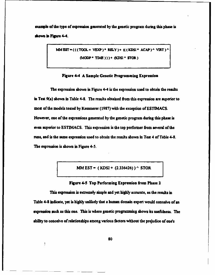
example of the type of expression generated by the genetic program during this phase is
shown 3 FIgure 4-4.
MMEST-(((TQOL+ VEXP) RELY)+ (((KDSI ACAP)A V3�T)A
(MODP TIME)))4 (KDSIA �QB�)
Figure 4-4 A Sample Genetic Programming Expression
The expression shown in Figure 4-4 is the expression used to obtain the results
in Test 9(a) shown in Table 44. The results obtained from this expression are superior to
morn of the models tested by Keminerer (1987) with the exception of ESTIMACS.
However, one of the expressions generated by the genetic program during this phase is
even superior to ESTIMACS. This expression is the top performer from several of the
runs, and is the same expression used to obtain the results shown in Test 4 of Table 4-8.
The expression is shown in Figure 4-5.
MM EST = (KDSI + (2.336426) ) A STOR
Figure 4-5 Top Performing Expression from Phase 2
This expression is extremely simple and yet highly accurate, as the results in
Table 44 indicate, yet is highly uniikely that a human domain expen would conceive of an
expression such as this one. This is wiiere genetic programming shows its usefihiness. The
ability to conceive of relationships among various factors without the prejudice of ones
80
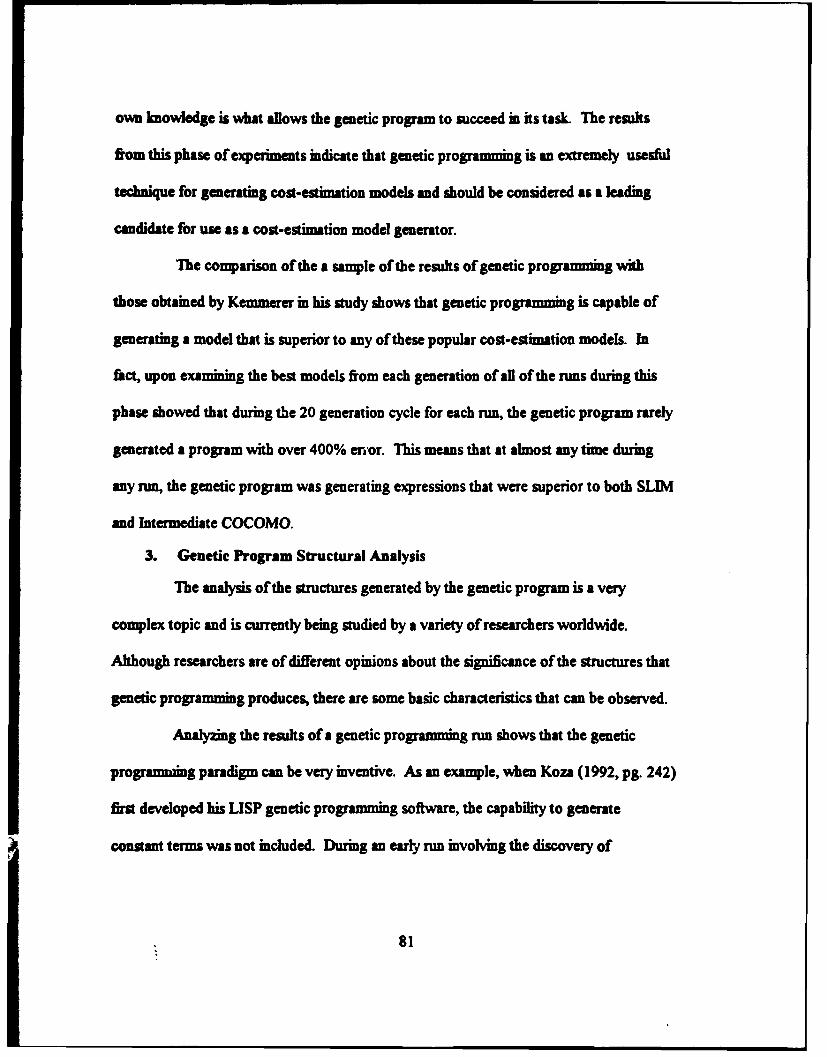
owe knowledge is what allows the genetic program to succeed in its task. The results
from this phase of experiments indicate that genetic programming is an extremely usesful
technique for generating cost-estimation models and should be considered as a leading
candidate for use as a cost-estimation model generator.
The comparison of the a sample of the results of genetic programming with
those obtained by Kemmerer in his study shows that genetic programming is capable of
generating a model that is superior to any of these popular cost-estimation models. In
f�ct, upon examining the best models from each generation of all of the nms during this
phase showed that during the 20 generation cycle for each nm, the genetic program rarely
generated a program with over 400% enor. This means that at almost any time during
any nm, the genetic program was generating expressions that were superior to both SLIM
and Intermediate COCOMO.
3. Genetic Program Structural Analysis
The analysis of the structures generated by the genetic program is a very
complex topic and is currently being studied by a variety of researchers worldwide.
Although researchers are of different opinions about the significance of the structures that
genetic programming produces, there are some basic characteristics that can be observed.
Analyzing the results of a genetic programming run shows that the genetic
programming paradigm can be very inventive. As an example, when Koza (1992, pg. 242)
first developed his LISP genetic programming software, the capability to generate
constant terms was not include& During an early run involving the discovery of
81
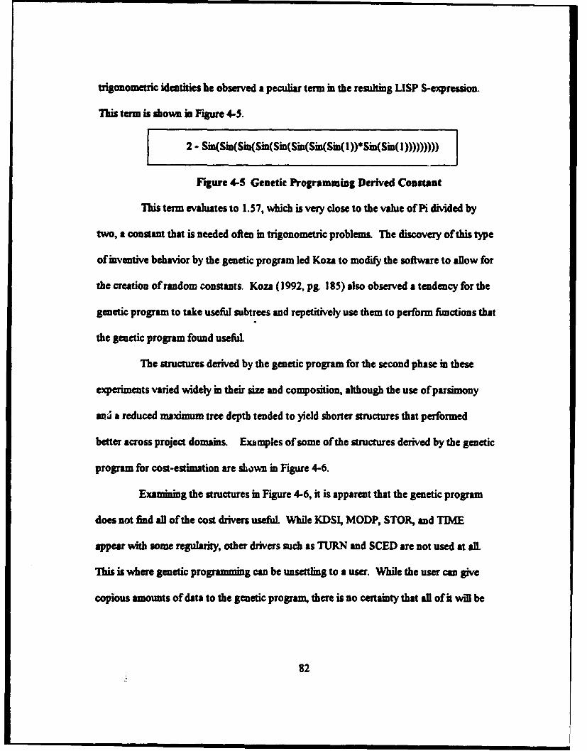
trigonometric identities he observed a peculiar term in the resulting LISP S-expression.
This term is shown in Figure 4-5.
[ 2 - Sin(Sin(Sin(Sin(Sin(Sin(Sin(Sin( !))" Sin(Sin(l)))))))))
Figure 4-5 Genetic Programming Derived Constant
This term evaluates to 1.57, which is very close to the value of Pi divided by
two, a constant that is needed often in trigonometric problem. The discovery of this type
of inventive behavior by the genetic program led Koza to modifly the software to allow for
the creation of random constants. Koza (1992, pg. 185) also observed a tendency for the
genetic program to take useful subtrees and repetitively use them to perform functions that
the genetic program found useful
The structures derived by the genetic program for the second phase in these
experiments varied widely in their size and composition, although the use of parsimony
avi a reduced maximum tree depth tended to yield shorter structures that performed
better across project domains. Examples of some of the structures derived by the genetic
program for cost-estimation are shown in Figure 4-6.
Examining the structures in Figure 4-6, it is apparent that the genetic program
does not find all of the cost drivers useful While KDSI, MODP, STOR, and TIME
appear with some regularity, other drivers such as TURN and SCED are not used at all
Mis is where genetic programming can be unsettling to a user. While the user can give
copious amounts of data to the genetic program, there is no certainty that all of it will be
82
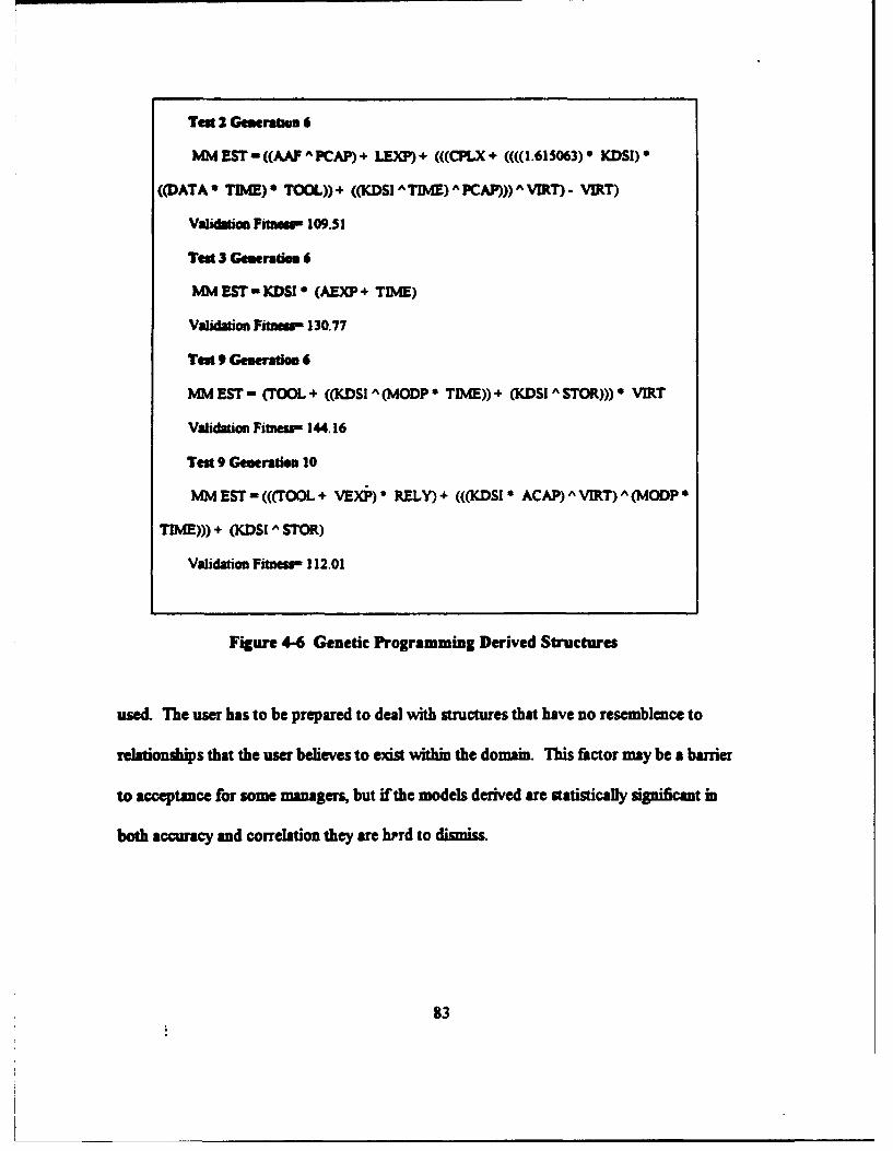
Test 2 Gemerabon 6
MM EST- ((AAF A PCAP) + LEXP).4 (((CPLX + ((((1.615063) $ KDSI)
((DATA * TIME) * TOOL)) + ((KDSI A TME) A PCAPV))) A VRrT) - VIRT)
Validtion Fitneas- 109.51
Test 3 Generation 6
MM EST - KDSI • (AEX.P + TIME)
Validation Fitness- 130.77
Test 9 Generatim 6
MM EST - (TOOL + ((KDSI A (MODP * TIME)) + (KDSi A STOA.))) • VIRT
Validation Fitness- 144.16
Test 9 Generation 10
MM EST - (((TOOL + VEXP) . RELY) + (((KDSI * ACAP) A VIRT) A (MODP *
TIME))) + (KDSI - STOR)
Validation Fitness- 112.01
Figure 4-6 Genetic Programming Derived Structures
used. The user has to be prepared to deal with structures that have no resemblence to
relationships that the user believes to exist within the domain. This factor may be a barrier
to acceptance for some managers, but if the models derived are statistically significant in
both accuracy and correlation they are hrrd to dismiss.
83
V. CONCLUSIONS AND RECOMMENDATIONS
A. CONCLUSIONS
The major objective of this thesis was to examine the effectiveness of three machine
learning techniques as applied to the field of software cost estimation. The driving factor
behind the investigation of machine learning in the cost estimation field is that current
software cost estimation models are both inaccurate and not very adaptable across
development domains. These are critical areas of weakness since the Department of
Defense is the largest single software consumer in the world, and it develops software for
a wide variety of domains. Therefore, it is necessary that a software cost estimation
model be both accurate and easily adaptable in order to be considered successful The
premise of this research was that there probably were relationships among the various
software project factors that the current models did not capture and that a machine
learning approach, where the models are derived directly from the data, may prove
superior in both performance and adaptability.
The three machine learning techniques studied in this thesis have all proven through
the experiments conducted to have great usefulness in the area of software cost
estimation. Each technique studied also brings to this field certain particular capabilities.
Neural networks showed a strong capability to capture and learn the project data, and
make estimates of reasonable accuracy that exhibited a high correlation with the project
actuals. When tested with data from outside the domain in which the networks were
84
developed, the neural networks showed a strong capability to generalize on the data that
was presented to them and make estimates that were superior to those of other
well-kmown models. This capability to make estimates across domains is critical when
seeking estimates on new projects with different development environments. Given the
limited amount of data that was available for testing the networks, they performed
surprisingly well. Neural networks also have an advantage in that they are relatively easy
to set up and train, and are certainly within the capabilities of most management persomel.
They also have the advantage of being self-calibrating, as long as the network is
maintained by continually retraining with data from newly completed projects. While not
as accurate as some of the algorithmic models, neural networks are certainly worthy of
consideration, especially since they have the ability to deal with non-numeric, or symbolic,
data. The best use of a neural network within an organization is probably at the earliest
stages where estimates that can at least capture the likely magnitude of a project are the
most useful.
The genetic algorithm experiments showed that they were higny effective as a tool
for model optimization and calibration. Given no more than a fitness function, a table of
literal values describing the projects, and a small amount of domain knowledge in the guise
of constraints on the fitness function, the genetic algorithm was able to find a complete set
of values for the cost drivers, coefficients, and exponents in the Intermediate COCOMO
model The resulting model values were shown to provide estimates that had a high
degree of accuracy and correlation for projects developed within the same domain, but
85
their performance was not as good when applied to projects outside of the domain in
which they were trained. Still, the genetic algorithm proved to be effective as a tool for
model calboration and it is easy to apply. The user has only to supply a fitness flmction
that includes the fitness measure, the model fimction and whatever constraints the user
fwels necessary for the particular domain. The power of evolution handles the search for
an optimal solution. Additionally, the genetic algorithm is highly extensible due to the
ability of the chromosome structure to be modified to reflect additional characteristics of
the domain. The genetic algorithm is likely to be of the greatest use in a situation where an
organization feels they have a model for how their development process finctions but they
need a method for calibrating the model to the data at hand. The genetic algorithm is very
capable in this situation.
In the third set of experiments the very new technique of genetic programming was
used as a means for model discovery. In this case, the only inputs provided were the
fitness measure, the project data, and a set of functions that were allowed to operate on
the data. Upon intializing the population with a random set of programs, the process of
evolution then generated models of greater and greater fitness as the genetic program
evolved through succeeding generations. The models resulting from this technique were
both highly accurate and strongly correlated. These results indicate that genetic
programming shows great usefulness as an exciting new approach to the cost estimation
problem and has probably the broadest range of uses of any of the techniques studied in
this thesis.
86

In all instances, each of the methods examined in this thesis was capable of generating
models that were competitive in both accuracy and correlation with other established cost
estimtion modelL In one case, the machine generated model outperformed all of the
more wellknown and established models. This level ofperformance exhibited by machine
generated models indicates that they should be given serious consideration by those
involved in the software development field, as they offer several advantages. First, they
directly reflect the data they are trained with, which automatically gives them an advantage
over a models that may have been developed outside of the domain in which it is being
applied. Second, they are highly extensible, meaning that any additional knowledge that
becomes available regarding the software development process can easily be incorporated
in these models. This provides an advantage over the more traditional models in that a
machine generated model is easily tailored to the data available. These advantages,
coupled with the performance levels noted in the experiments conducted in this study
indicate that machine learning is an effective and useful technique for the field of software
cost estimation.
B. RECOMMENDATIONS FOR FURTHER RESEARCH
There are several areas that are candidates for further research based on this study.
First, additional experiments can be conducted to extend the level of kmowledge regarding
how each of the techniques should be applied to achieve the greatest effectiveness.
Secondly, research can be conducted into coupling these machine learning techniques
together in order to create a suite of tools that may be able to provide a superior level of
87

performance. As an example, one could build an expert system front end that could query
a user about project characteristics in order to populate a data base. This expert system
frort end could then be coupled to a neural network that could provide general estimates,
or it could be coupled to the genetic program, which could generate candidate models It
may also be possible to have a neural network monitor the results of the models the
genetic program develops, and make a selection as to which model is best for a particular
situation based on the user's inputs the expert-system front-end. Fmally, a similar set of
experiments to those conducted in this study could be performed using data from a variety
of domains for training. This may prove insightful, since a certain amount of
meta-knowledge about the data would have to be apparent in any models developed using
these techniques.
88
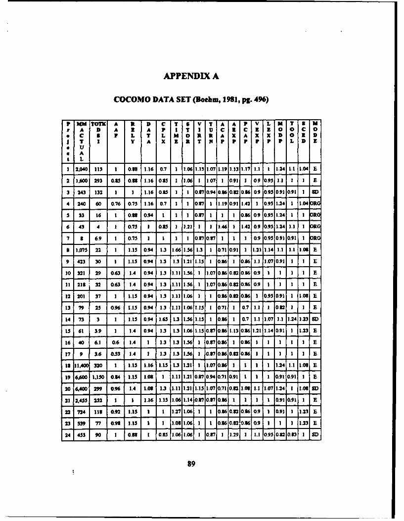
APPENDIX A
COCOMO DATA SET (Boehm, 1981, pg. 496)
P MM TOTK A R D C T 5 V T A A P V L N T 8 NA D A 1 A F I T I U C I C Z 1 0 0 C OC 3 F L T L M O R R A X A X X DO [ D
J T I v A X RUIt T N F P P F F P L D 2* U
* At L
1 2.040 113 1 0.31 1.16 0.7 1 1.06 1.15 1.07 1.19 1.13 1.17 1.1 1 1.24 1.1 1.04 E
2 1.600 293 0.35 0.33 1.16 0.15 1 1.06 1 1.07 1 0.91 1 0.9 0.95 1.1 1 1 E
3 243 132 1 1 1.16 0.8.5 1 1 0.37 0.94 0.86 0.82 0.36 0.9 0.95 0.91 0.91 1 51)
4 240 60 0.76 0.75 1.16 0.7 1 1 0.37 1 1.19 0.91 1.42 1 0.95 1.24 1 1.04 0
5 33 16 1 0.8 10.94 1 1 1 0.87 1 1 1 0.8610.9 0.95 1.241 1 al
6 43 4 1 0.75 1 0.35 1 1.21 1 1 11.46 1 1.42 0.9 0.95 1.24 1.1 1 1
7 8 6.9 1 0.75 1 1 1 1 0.870.871 1 1 0.9 0.95 0.91 0.91 1 1
1 1.075 22 1 1.15 0.94 1.3 1.66 1.56 1.3 1 0.71 0.91 1 1.21 1.14 1.1 1.1 1.08 E
9 423 30 1 1.15 0.94 1.3 1.3 1.21 1.15 1 0.36 1 0.86 1.1 1.07 0.91 1 1 E
10 321 29 0.63 1.4 0.94 1.3 1.11 1.56 1 1.07 0.86 0.82 0.86 0.9 1 1 1 1 E
11 218 32 0.63 1.4 0.94 1.3 1.11 1.56 1 1.07 0.360.32 0.36 0.9 1 1 1 1 E
12 201 37 1 1.15 0.94 1.3 1.11 1.06 1 1 0.86 0.82 0.86 1 0.95 0.91 1 1.03 E
13 79 25 0.96 1.15 0.94 1.3 1.11 1.06 1.15 1 0.71 I 0.7 1.1 1 0.32 I 1 E
14 73 3 1 1.15 0.94 1.63 1.3 1.56 1.15 1 0.86 1 0.7 1.1 1.07 1.1 1.24 1.23 SD
15 61 3.9 1 1.4 0.94 1.3 1.3 1.06 1.15 0.37 0.36 1.13 0.86 1.21 1.14 0.91 1 1.23 E
16 40 6.1 0.6 1.4 1 1.3 1.3 1.561 1 0.870.36 1 0.861 1 1 1 1 E
17 9 3.6 0.53 1.4 1 1.3 1.3 1.36 0.8710.60.2 0.36 1 I 1 1 I E
13 111.4 320 1 1.115 1.16 1.15 1.3 1.21 1 1.07 0.86 1 1 1 1 1.24 1.1 1.08 E
19 6.600 1.150 0.34 1.15 1.08 1 1.11 1.21 0.7 0.94 0.71 0.91 1 1 1 0.91 0.91 1 E
20 6.400 299 0.96 1.4 1.03 1.3 1.11 1.21 1.15 1.07 0.71 0.32 1.08 1.1 1.07 1.24 1 1.08 SD
21 2,455 252 1 1 1.16 1.15 1.06 1.14 0.87 0.37 0.36 1 1 1 1 0.91 0.91 1 E
22 724 i13 0.92 1. 1 1 1.27 1.06 1 1 0.86 0.82 0.86 0.9 1 0.91 1 1.23 E
23539 77 0.91 1.15 1 1 1.03 1.061 1 0.86 0.8210.86 0.91 1 1 1.23 E
24453 90 1 0.31 I 0..5 1.06 1.06 1 0.7 1 1.291 1 1. 0.95 0.120.13 1 SD
89
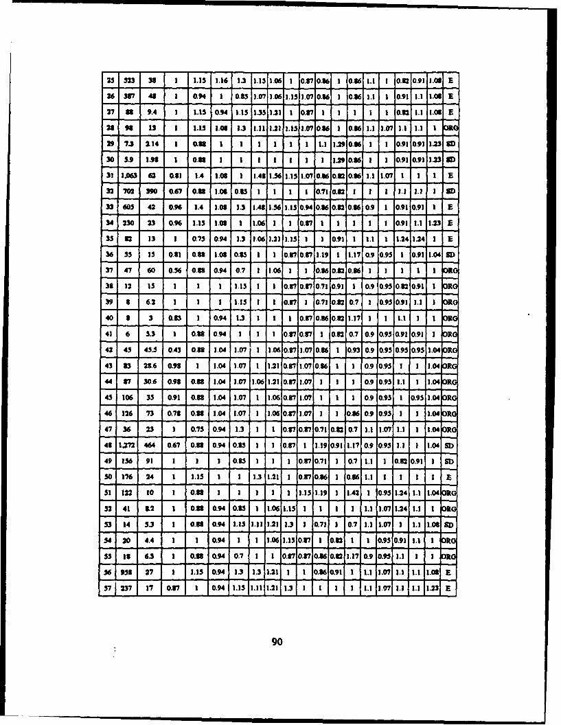
25 523 38 1 1.15 1.16 13 1.1311.06 1 0.8710.86 1 0.36 1.1 1 0.3 0.91 1.06 E
26 337 48 1 0.94 1 0.33 1.071 06 1.15 1.07/0.86 1 0.86 1.1 1 0.91 1.1 1.06 E
27 33 9.4 1 1.15 0.94 1.15 1.351.21 1 0.871 1 1 1 1 0.22 1.1 1.00 E
28 9 13 1 1.15 1.06 1.3 1.11 1.21 .135 1.0710.86 1 0.86 1.1 1.07 1.1 1.1 11 ORQJ
29 7.3 2.14 1 o.33 I I 1 I I 1 1.1 1.290.861 1 0.910.911.23 SD
305 .9 1.96 1 0.33 1 1 1 1 1 1 1." 0.86 1 1 0.910.911.23S
31 3.063 62 0.S 1.4 1.06 1 1.43 1.56 1.15 1.07 0.86 0.32 0.86 1.1 1.07 1 1 1 E
32 702 3O 0.67 0.3 1. 0683 1 1 1 10.7 o 0. 1 1 1 .1 1. 1 SD
33 W30 42 0.96 1.4 1.0i 3.3 1.48 1.56 1.15 0.94 0.86 0.2 0.86 09 1 0.91 091 1 E
34 230 23 0.96 1.15 1.s 1 1.061 1 1 0.71 1 1 1 1 1 0.91 1.1 JM E
35 32 13 1 0.73 0.94 3.3 3.06 1.21 1.15 1 1 0.91 1 11.1 1 1.24 1.24 1 E
36 55 15 0.81 0.31 1.06 0.35 1 1 0.87 0.87 1.19 1 1.17 0.9 0.95 1 0.91 1.041 SD
37 47 60 0.%5 0.33 0.94 0.7 1 3.06 3 1 0.36 0.32 0.36 1 1 1 1 1 R
38 12 Is 1 I 1 1.15 1 1 0.87 0.37 0.71 0.91 1 0.9 0.95 0.M3 0.91 1 11
39 3 6.2 1 1 1 1.135 I 0.37 1 0.7110.3 0.7 1 0.95 0.91 1.1 1 R0
403 3 0.83 1 0.94 13 1 1 1 80.370.860.3 1.171 1 1.1]1 1 RG
41 6 .5.3 1 0.-0 0.94 1 1 1 0.37 0.87 1 0.32 0.7 0.9 0.95 0.91 0.91 1 "K
42 45 45.5 0.43 0.33 1.04 1.07 1 .1.06 0.37 1.07 0.36 1 0.3 0.9 0.9510.95 0.9511.404 RO
43 83 23.6 0.98 1 1.04 1.07 1 1.21 0.37 1.07 0.86 1 1 0.9 0.95 1 1 1.04 1R
44 37 30.6 0.93 0.33 1.04 3.07 1.06 1.21 0.87 3.07 1 1 1 0.9 0.95 1.1 1 1.04 0
45 106 35 0.91 0.83 1.04 1.07 1 1.06 0.7 1.071 I 1 1 0.9 0.95 1 0.95 1.04 1Km
46 126 73 0.78 0.33 1.04 1.07 3 1.06 0.3713.07 1 1 0.36 0.9 0.93 1 1.04 OR
47 36 23 1 0.75 0.94 1.3 1 1 0.37 0.8710.71,0.82 0.7 1.1 1.07 1.1 1 1.04 oKG
43 1,272 464 0.67 0.33 0.94 0.83 1 1 0.37 1 1.19 0.91 1.17 0.9 0.93 3.1 1 1.04 SD
49 16 91 3 1 1 0.8351 1 110370.7110.71.110. 0.911 SD
50 176 24 1 1.15 1 1 1.3 1.21 1 0.87 0.86 1 0.36 1.11 1 1 1
51 122 10 1 0.38 1 1 31 1 1 31.15 1.191 1 i.42 1 0.9.24 1.1 1.04o
52 41 32 1 0.3 0.94 0.35 1 1061.11 1 1 1 1 1.11.071.24 1.1 1 I53 14 5.3 1 0.33 0.94 1.135 1.11 1.21 3.3 1 0.71 3 0.7 13.1 11.07 1 1.1 1.06 SD
44 20 4.4 1 1 0.94 1 1 1.06.15 0.37 1 0.C3 1 1 0.95 0.91 1.1 1 .
55 18 63 1 0.01 0.94 0.7 1 ! 0.37 0.37 0.36 0.32 3.17 0.9 0.953 1.1 3 O1
M 6 58 27 3 1.13 10.94 1.3 1.3 1.21 1 1 0.8610.91 1 1.1 1.07 1.1 1.1 1.03 E
37 j237 17 0.37 1 0.94 1.15 1.11 1.21 1.3 1 1 1 1 1.3 1.07 1.1 1.1 1.231 E
90
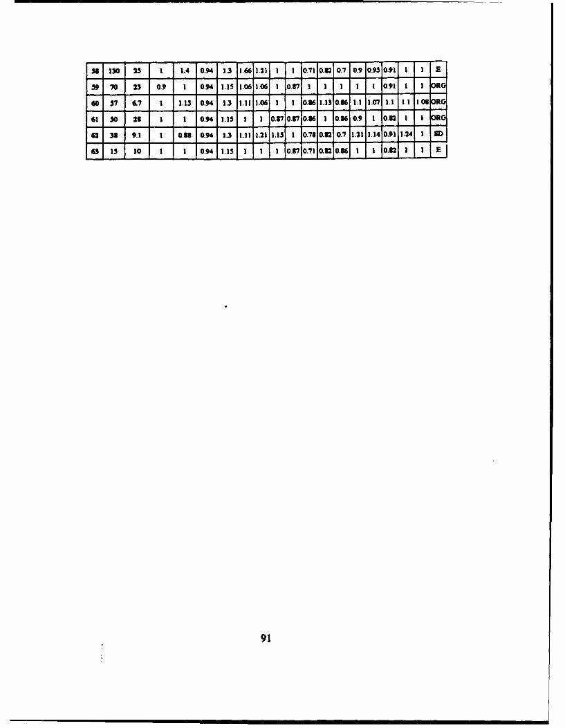
so 130 25 1 1.4 0.94 1.3 1.66 1.21 1 1 0.71 0.82 0.7 0.9 0.95 0.91 1 1 E
59 70 23 0.9 1 0.94 1.15 1.06 1.06 1 0.371 1 1 1 1 0.91 1 1 ORG
60 57 &7 1 1.13 0.94 1.3 1.11 1.06 1 1 0.86 1.13 0.36 1.1 1.07 1.1 1.1 1I.06ORO
61 30 23 I 1 0.94 1.15 I 1 0.87 o.7 0.86 1 0.36 0.9 1 0.M32 I i RCI
62 9.1 1 0.88 0.94 1.3 1.11 1.21 1.15 1 0.73 0.82 0.7 1.21 1.14 0.91 1.24 1 3± D
6 15 10 1 i 0.941 .15 1 !0.70.7110.8210.36 1 1 0.31 1 E!
91
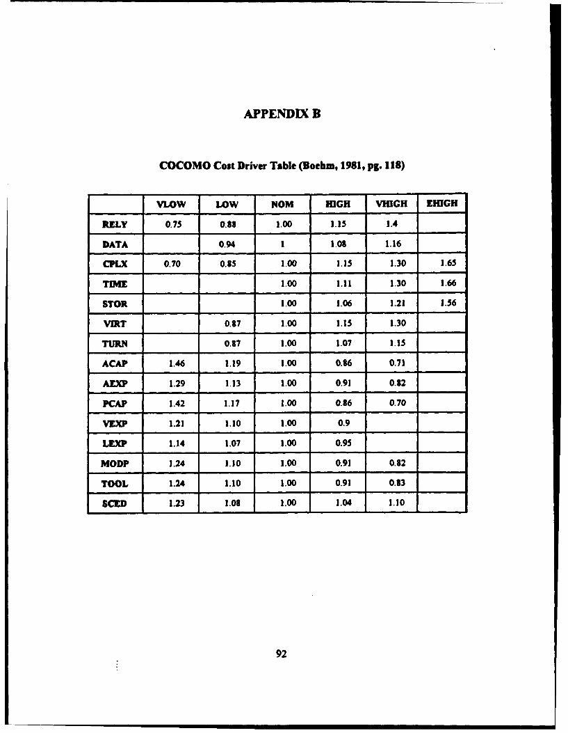
APPENDIX B
COCOMO Cost Driver Table (Boehm, 1981, pg. 118)
VLOW LOW NOM HIGH VmGH EHIGH
RELY 0.75 0.88 1.00 1.15 1.4
DATA 0.94 1 1.08 1.16
CPLX 0.70 0.85 1.00 1.15 1.30 1.65
TIME 1.00 1.11 1.30 1.66
STOR 1.00 1.06 1.21 1.56
VIRT 0.87 1.00 1.15 1.30
TURN 0.87 1.00 1.07 1.15
ACAP 1.46 1.19 1.00 0.86 0.71
AEXP 1.29 1.13 1.00 0.91 0.82
PCAP 1.42 1.17 1.00 0.86 0.70
VEXP 1.21 1.10 1.00 0.9
LEXP 1.14 1.07 1.00 0.95
MODP 1.24 1.10 1.00 0.91 0.82
TOOL 1.24 1.10 1.00 0.91 0.83
SCED 1.23 1.08 1.00 1.04 1.10
92
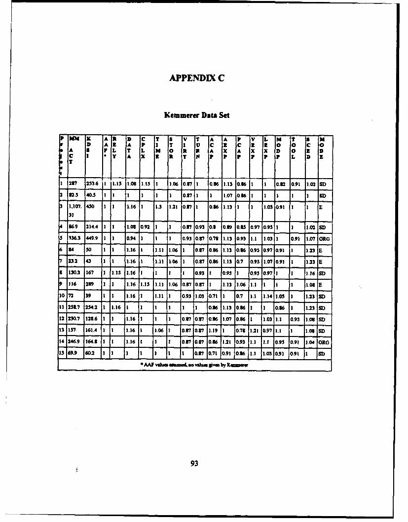
APPENDIX C
Kemmerer Data Set
I 1.1 1.03 1.15 1 1.06 0.37 ! 0.36 1 0.32 0.91 1.02
23 82.5 40.5 1 11 1 1 1 1 0.87 1 1 1.0710.861 1 1 1 SD
3 1.107. 450 1 1 1.1611 1.3 1.21 0.37 1 0.86 1.13 1 1 1.03 0.91 1 1 E
31
86.9 214.4 1 1 1.03 0.92 1 1 0.37 0.93 0.8 0.39 0.35 0.97 0.95 1 1 1.02 SD
5 336.3 449.9 1 1 0.94 1 1 1 0.93 0.87 0.78 1.13 0.93 1.1 1.03 1 0.91 1.07 ORG
6 84 so 1 1 1.16 1 1.11 1.06 1 0.1 7 0.86 1.13 0.36 0.95 0.97 0.91 1 1.23 E
7 23.2 43 1 1 1.16 1 I.M1 1.06 11 0.87 0.86 1.13 0.7 0.95 1.07 0.91 1 1.23 E
8 130.3 167 1 11.15 1.16 1 i I 1 0.93 i 0.95 I 0.95 0.97 1 1 1.16 SD
9 116 239 11 1 1.16 1.15 1.11 1.06 0.37 0.37 1 1.13 11.06 1.1 1 1 1 1.08 E
10 72 39 1 1 1.16 1 1.11 1 0.93 1.03 0.71 1 0.7 1.1 1.14 1.05 1 1.23 SD
It 1251.7 254.2 1 1.161 1 1) 1 1 11 0.36 1.13 0.86 1 1 0.86 1 1.23 SD
12 230.7 128.6 1 1 1.16 1 I 1 0.87 0.37 0.36 1.07 0.36 1 1.03 1.1 0.95 1.03 SD
13 157 161.4 1 1 1 .16 I1 1.06 1 0.37 0.87 1.19 1 0.78 1.21 0.97 1.1 1 1.08 SD)
14 246.9 164.8 I 1 1.16 1 1 1 0.37 0.37 0.86 1.21 0.93 1.1 1.1 0.95 0.91 1.04 ORG
15 69.9 60.2 1 1 1 1 1 0.V7 0.71 0.91 0.36 1.1 1.03 0.91 0.91 SD
"AAF valuta mn no valut ivm by R•insw
93

APPENDIX D
COCOMO T7]INIMG AND TESTING DATA SETS
TRAINING DATA SETP MM TOT A R D C T 5 V T A A P V L M T 3 M
vA K A R A FPIT I V CI C 2 100CC0SC D F L T L M 0 A X A XX D 0 D
T 2 Y A X Z i T M F F P P P P L D I* U i
€ At L
1 2,040 113 1 0.3 1.16 0.7 1 1.06 1.15 1.07 1.19 1.13 1.17 1.1 1 1.24 1.1 1.04 E
3 243 132 1 I 1.16 0.45 1 1 0.87 0.94 0.86 0.32 0.36 0.9 0.95 0.91 0.91 1 SD
4 240 60 0.76 0.75 1.16 0.7 1 1 0.87 1 1.19 0.91 1.42 1 0.95 1.24 1 1.04 RG
5 33 16 1 0.8 0.94 11 1 0.'71 1 1 0.86 0.9 0.95 1.241 1 OR
9 423 30 1.1-5 0.94 1.3 1.3 1.21 1.15 1 0.86 1 0.86 1.1 1.07 0.911 I E
10 321 29 0.63 1.4 0.94 1.3 1.11 1.-56 1 1.07 0.36 0.832 0.86 0.9 1 i 1 1 E
11 218 32 0.63 1.4 0.94 1.3 1.11 1.56 1 1.07 0.86 0.832 0.36 0.9 1 I I 1E
16 40 6.1 0.6 1.4 1 .3 1.3 1.56 1 0.8710.86 1 0.86 1 1 1 1 1 F
20 6.400 299 0.96 1.4 1.08 1.3 1.11 1.21 1.15 1.07 0.71 0.82 1.06 1.1 1.07 1.24 1 1.08 SD
21 2.455 252 1 1 1.16 1.15 1.06 1.14 0.37 0.3 0.86 1 1 1 1 0.91 0.911 1 E
22 724 118 0.92 1.13 1 1 1.27 1.06 1 I 0.36 0.82 0.36 0.9 1 0.91 1 12.3 1E
23 539 77 0.93 1.15 1 1 1.0311.06 1 1 0.8610.32 0.36 0.9 1 1 1 1.231
24 453 90 1 0.33 I 0.85 1.061.06 1 0.37 1 1.29 1 1.1 0.95 0.32 0.833 1 SD
25 523 33 1 1.15 1.16 1.3 1.15 1.061 1 0.837 0.86 1 0.86 1.1 1 0.03 0.91 1.08 E
26 337 48 1 0.94 1 0.85 1.07 1.06 1.15 1.07 0.86 1 0.36 1.1 1 0.91 1.1 1.06 E
238 9 13 1 1.15 1.08 1.3 1.11 1.21 1.1-5 1.07 0.86 1 0.86 1.1 1.07 1.1 1.1 1 3R0
31 1063 M 62 0.81 1.4 1.06 1 1.48 1.56 1.15 1.07 0.36 0.83 0.86 1.1 1.07 1 1 1 E
32 702 390 0.67 0.88 1.03 0.351 1 1 1 0.71 0.8321 1 1 1.1 1.1 1 SD
33 603 42 0.96 1.4 1.06 1.3 1.43 1.56 1.15 0.94 0.86 0.83 0.86 0.9 1 0.91 0.91 1E
34 230 23 0.96 1.15 1.0 1 11.061 1 1 0.3 1 1 1 I 1 0.91 1.1 1.31 E
35 3 13 1 0.75 0.94 1.3 1.061.211.15 1 1 0.91 1 1.1 1 1.24 1 E
36 5- 5 15 0.1 0.88 1.08 0.835 1 0.37 0.37 1.19 1 1.17 0.9 0.95 1 0.9131.04 SD
94
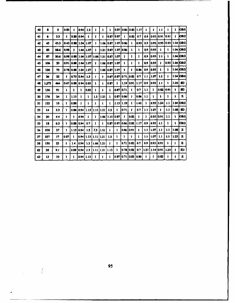
40 8 3 0.0 1 0.94 13 1 1 1 0.30.3160.382 1.17 1 1 1.1 I K ORG
41 6 5.31 0.3 O 0.94 1 1 1 0.37 0.37 I 0.32 0.7 0.9 0.95 0.91 0.9 1 ORO
42 45 45.5 0.43 0.33 1.04 1.07 1 1.06 0.37 1.07 0.36 1 0.93 0.9 0.95 0.95 0.95 1.04 ORO
4 831 13 1 0.93 1 1.04 1.071 1 .2110.3711.07 0.86 1 1 0.9 0.95 1 1 1.04 0O
44 37 30.6 0.93 0.33 1.04 1.07 1.06 1.21 0.37 1.07 1 1 1 0.9 0.95 1.1 1 1.04 0.O
45 106 35 0.91 0.3 1.04 1.07 1 1.06 0.37 1.07 1 1 1 0.9 0.95 1 0.95 1.04 OR0
46 126 73 0.78 0.W 1.04 1.07 1 1.06 0.371.07 1 1 0.36 0.9 0.95 1 1 11.04 ORO
47 36 23 1 10.73 0.94 1.3 I 1 0.370.7. 0.71 0.32 0.7 1.1 1.07 1.1 1 1.04 0ORG
43 13272 464 0.67 0.3 0.94 0.35 1 1 0.37 1 1.19 0.91 1.17 0.9 0.95 1.1 1 1.04 ED
49 156 91 1 I 1 0.85 1 1 1 0.7 0.71 1 0.7 1.1 1 0.82 0.91 1 SD
50 176 24 1 1.15 1 1 1.3 1.21 1 0. 0.86 1 0.36 1.11 1 1 1 EF
51 122 10 1 0. 1 I I I I 1 1.15 1.19 1 1.42 1 0.95 1.24 .1 1.0410H O
53 14 5.3 1 0.88 0.94 1.15 1.11 1.21 1.3 1 0.71 1 0.7 1.1 1.07 1 1.1 1.06 SID
54 20 4.4 1 1 0.94 1 1.06 1.130.37 1 0.32 1 1 0.9510.91 1.1 1 KOG
35 13 6.3 1 0.3 0.94 0.7 1 1 0.87 0.37 0.86 0.82 1.17 0.9 0.95 1.1 1 1 OitG
56 958 27 1 1.13 0.94 1.3 r.3 1.21 1 1 0.36 0.91 1 1.1 1.07 1.1 1.1 1.08 E
37 237 17 0.87 1 0.94 1.15 1.11 1.21 1.3 1 1 1 1 1.1 1.07 1.1 1.1 1.23 E
38 130 25 1 1.4 0.94 1.3 1.66 1.21 1 1 0.71 0.82 0.7 0.9 0.95 0.91 1 1 E
62 38 9.1 1 O.3 0.94 . 1.11 1.21 1.15 1 0.73 0.32 0.7 1.21 1.14 0.91 1.24 1 SD
63 15 10 1 ±10.94 1.151 I I 0.37 0.71 0.82 0.86 1 1 0.82 E
95
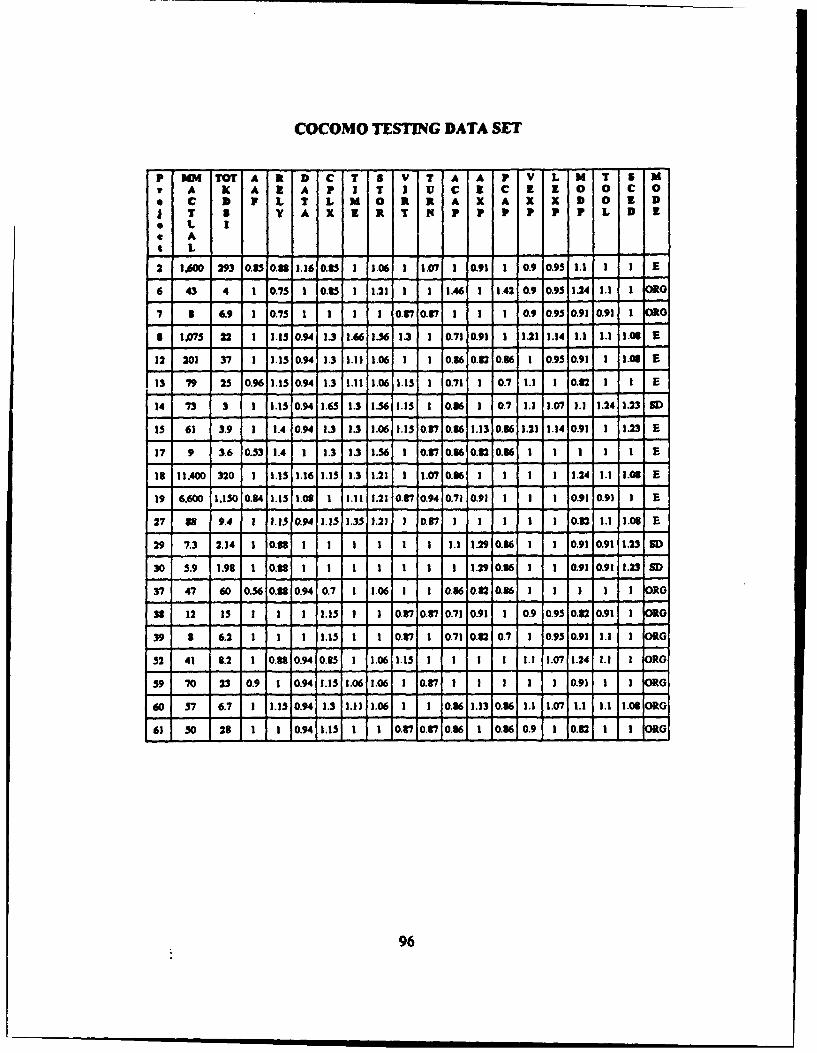
COCOMO TESTING DATA SET
P MM TOT A R D C T 5 V T A A P V L M T S MA K A I A P I T I U C Z C R 3 00 Co
* C D L T L M O R R A X A X X D 3 0 DT 8 V A X U R T N P P P P•P P L D l
* 1. I
* AL L
2 1A600 293 0.15 0.83 1.16 0.31 3 3.06 1 1.07 1 0.91 1 0.9 0.95 1.1 1 1 E1
6 43 4 1 0.75 1 0.3511 .211 1 1.461 1.42 0.9 0.95 1.24 1. 1 03*
7 a 6.9 1 0.75 1 1 1 1 0.87 0.37 1 1 I 0.9 0.95 0.91 0.91 1 OR0
8 1,075 22 1 1.1510.94 13 1.66 11.56 13 1 0.71 0.91 1 1.21 1.14 1.1 1.1 1.06 E
12 201 37 1 1.15 0.94 1.3 1.11 1.06 1 1 0.36 0.82 0.86 1 0.95 0.91 1 1.08 E
13 79 25 0.96 1.15 0.9411.3 1.11 1.06 1.13 1 0.71 1 0.7 1.1 1 0.82 I 1 E
14 73 3 !1 1.15 0.94 1.65 1.3 1.56 1.15 1 0.86 1 0.7 1.1 1.07 1.1 1.24 1.23 SD
is 61 3.9 1 1.4 0.94 1.3 1.3 1.06 1.13 0.3710.36 1.13 0.36 1.21 1.14 0.91 1 1.23 E
17 9 3.6 0.53 1.4 1 1.3 1.3 1.56 1 0.9710.36 0.32 0.861 1 1 1 1 E
18 11.400 320 1 1.5 1.16 1.15 1.3 1.21 1 1.07 0.86 1 1 1 I 1.24 1.1 1.08 E
19 6.600 1.150 0.34 1.15 1.08 1 1.11 1.21 0.87 0.94 0.71 0.91 1 I 1 0.91 0.91 3 1 E
27 8 1 9.4 1 1.1530.94 1.15 1.35 1..21 1 0.371 1 1 1 1 1 0.321.1 1.086 E
29 7.3 2.14 1 0.8 I I I I I 1 1.1 1.9 0.86 1 1 0.91 0.91 1.23 SD
30 1.9 1.9 3 1 0.8 I ! I I I 1 1 1.29 0.86 1 I 0.91 0.91 1.23 SD
37 47 60 0.560.3 0.94 0.7 i 1.06 I 1 0.86 0.82 0.36 1 1 3 1 ORO
38 12 15 1 1 1 1.15 1 1 0.37 0.87 0.71 0.91 1 0.9 0.95 0.82 0.91 1 oRr
39 3 6.2 1 1 1 1.15 1 11 0.37 1 0.71 0.8210.7 1 0.9510.91 1.1 I ORG
52 41 8.2 1 0.83 0.94 0.35 1 1.06 1.15 1 1 1 1 1.1 1.07 1.24 1.1 1 DRG
59 70 23 0.9 1 0.94 1.15 1.061.06 1 0.87 1 1 1 1 1 0.911 1 KRG
60 37 6.7 I 1.15 0.94 1.3 1.11 1.06 1 1 0.86 1.13 0.86 1.1 1.07 1.1 1.1 1.03 ORG
61 .50128 1 1 0.94 1.151 0.37Y0.7 0.8610.60.9 1 0.821 1G
96
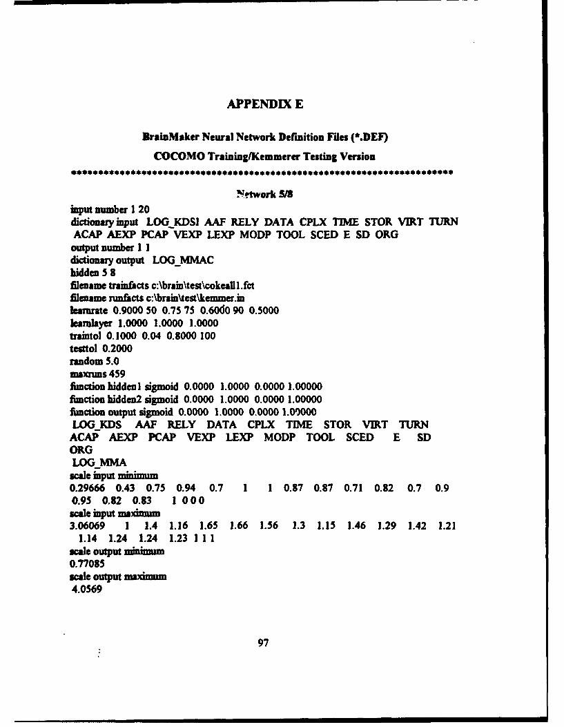
APPENDIX E
BrainMaker Neural Network Definition Files (*.DEF)
COCOMO Training/Kemmerer Testing Version
Network /8
input number 1 20dictionary input LOG KDSI AAF RELY DATA CPLX TAE STOR VIRT TURNACAP AEXP PCAP VEXP LEXP MODP TOOL SCED E SD ORG
output number I Idictionary output LOG MMAChidden 5 8filename trainfacts c:\brain\test\cokeall.fctJilename rnfacts c:\brain\test\kemmer.inleararate 0.9000 50 0.75 75 0.6060 90 0.5000learalayer 1.0000 1.0000 1.0000traintol 0.1000 0.04 0.8000 100testtol 0.2000random 5.0maxumms 459fiuction hidden] siSmoid 0.0000 1.0000 0.0000 1.00000flmction hidden2 sigmoid 0.0000 1.0000 0.0000 1.00000function output sigmoid 0.0000 1.0000 0.0000 1.0I000LOGKDS AAF RELY DATA CPLX TIME STOR VIRT TURN
ACAP AEXP PCAP VEXP LEXP MODP TOOL SCED E SDORGLOGMMA
scale input minimum0.29666 0.43 0.75 0.94 0.7 1 1 0.87 0.87 0.71 0.82 0.7 0.90.95 0.82 0.83 1 000scale input madnu3.06069 1 1.4 1.16 1.65 1.66 1.56 1.3 1.15 1.46 1.29 1.42 1.21
1.14 1.24 1.24 1.23 111scale output minimm0.77085scale output maMIM4.0569
97
-- .am i i mama i~iass ilm i iliI ==MIIM

Network 8/9
input number 1 20dictionary input LOGKDSI AAF RELY DATA CPLX TIME STOR VIRT TURNACAP AEXP PCAP VEXP LEXP MODP TOOL SCED E SD ORG
output number I Idictionary output LOG MMAChidden 8 9filename trainfacts c:\brain\test\cokealll.fctfilename rnfacts c:\brain\test\kemmer.inlearurate 0.9000 50 0.75 75 0.6000 90 0.5000leamilyer 1.0000 1.0000 1.0000traintol 0.1000 0.04 0.8000 100testtol 0.2000random 5.0maxrms 430finction hiddenl sigmoid 0.0000 1"0000 0.0000 1.00000fumction hidden2 sigmoid 0.0000 1.0000 0.0000 1.00000fimction output sigmoid 0.0000 1.0000 0.0000 1.00000LOG KDS AAF RELY DATA CPLX TIME STOR VIRT TURN
ACAF AEXP PCAP VEXP LEXP MODP TOOL SCED E SDORGLOG MMA
scale input minimum0.29666 0.43 0.75 0.94 0.7 1 1 0.87 0.87 0.71 0.82 0.7 0.90.95 0.82 0.83 1 000
scale inpt maximum3.06069 1 1.4 1.16 1.65 1.66 1.56 1.3 1.15 1.46 1.29 1.42 1.21
1.14 1.24 1.24 1.23 11 1scale output minimum0.77085scale output4.0569
98
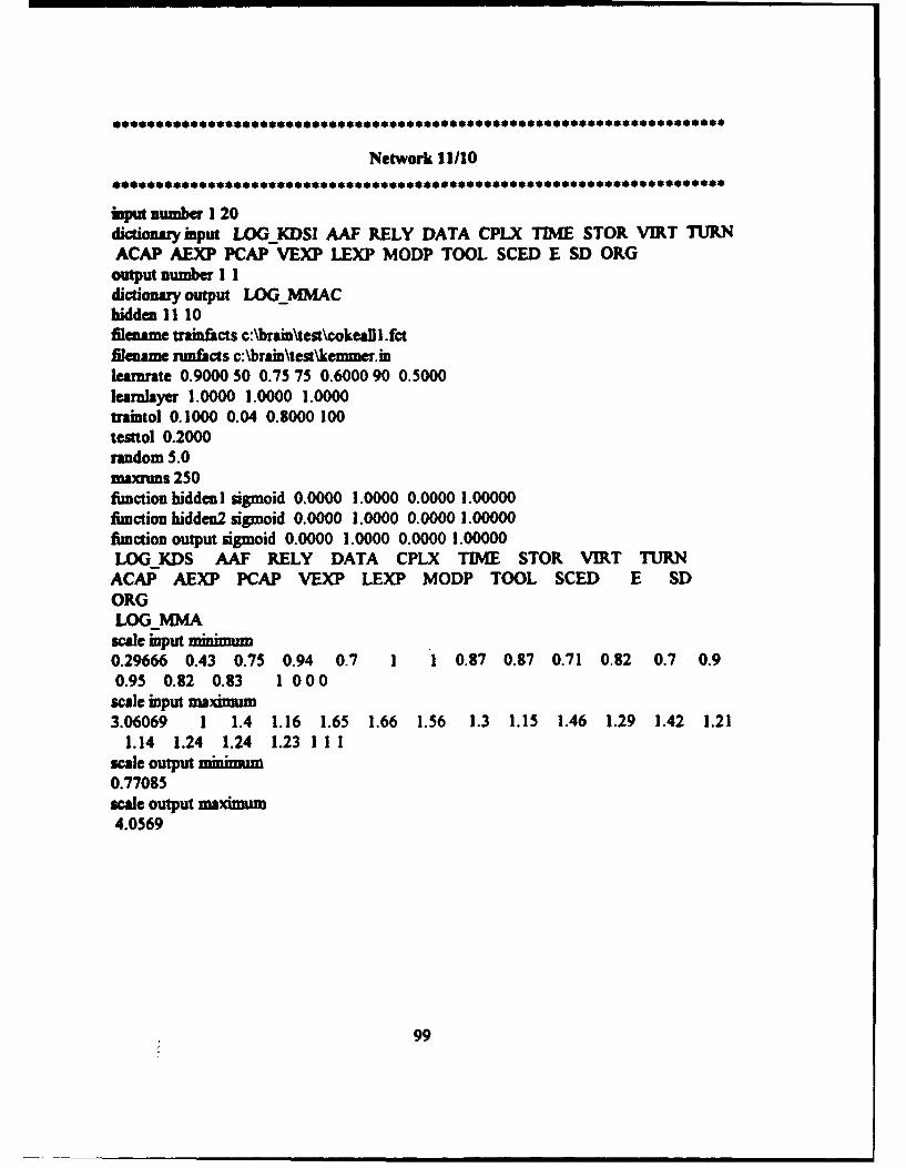
Network 11/10
finput number 1 20dictionary imput LOGKDSI AAF RELY DATA CPLX TIME STOR VIRT TURNACAP AEXP PCAP VEXP LEXP MODP TOOL SCED E SD ORGoutput number I 1dictionary output LOG_MMAChidden 11 10filename trainfacts c:\brain\test\cokealll.fctfilename runfacts c:\brain\tes\kemmer.inlearnrate 0.9000 50 0.75 75 0.6000 90 0.5000leanlayer 1.0000 1.0000 1.0000traintol 0.1000 0.04 0.8000 100testtol 0.2000random 5.0maxmms 250fimction hidden I sigmoid 0.0000 1.0000 0.0000 1.00000flnction hidden2 sigmoid 0.0000 1.0000 0.0000 1.00000flmction output sigmoid 0.0000 1.0000 0.0000 1.00000LOG KDS AAF RELY DATA CPLX TIME STOR VIRT TURN
ACAP AEXP PCAP VEXP LEXP MODP TOOL SCED E SDORGLOG MMAscale input minimum0.29666 0.43 0.75 0.94 0.7 1 1 0.87 0.87 0.71 0.82 0.7 0.90.95 0.82 0.83 1 000
scale input maximum3.06069 1 1.4 1.16 1.65 1.66 1.56 1.3 1.15 1.46 1.29 1.42 1.21
1.14 1.24 1.24 1.23 1 11scale output minimum0.77085scale output maximum4.0569
99
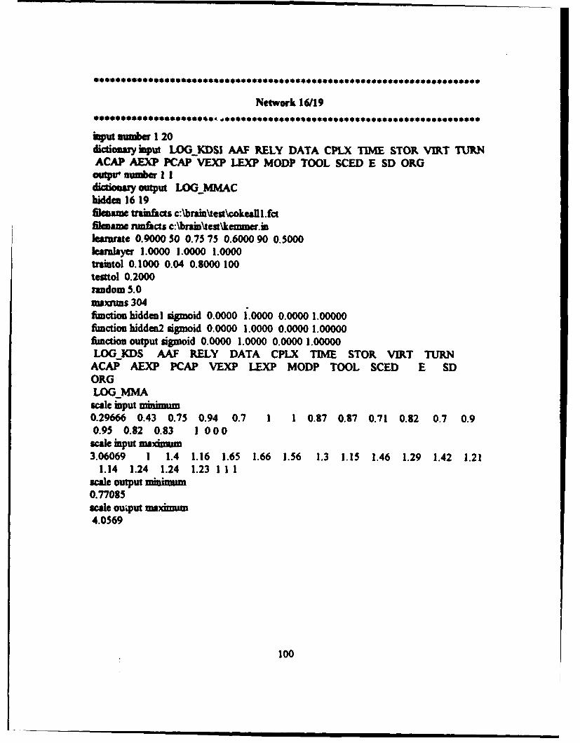
Network 16/19
aput numbe 1 20dictioary input LOGKDSI AAF RELY DATA CPLX TIME STOR VIRT TURNACAP AE" PCAP VEXP LEXP MODP TOOL SCED E SD ORGoutpu number I Idictionazy output LODGMMAChiddem 16 19filaaame trainfacts c:\brain\test\cokeall.fctfilename ninfacts c:\brain\test\kemmer.inlerniate 0.9000 50 0.75 75 0.6000 90 0.5000emadyer 1.0000 1.0000 1.0000
traintol 0.1000 0.04 0.8000 100tesuol 0.2000random 5.0nm,•ins 304fuiction hidden I sigmoid 0.0000 1.0000 0.0000 1.00000fimction hidden2 sigmoid 0.0000 1.0000 0.0000 1.00000finction output sigmoid 0.0000 1.0000 0.0000 1.00000LOG KDS AAF RELY DATA CPLX TIME STOR VIRT TURN
ACAP AEXP PCAP VEXP LEXP MODP TOOL SCED E SDORGLOG MMA
scale input minimum0.29666 0.43 0.75 0.94 0.7 1 1 0.87 0.87 0.71 0.82 0.7 0.90.95 0.82 0.83 1 000
scale input ma xmu3.06069 1 1.4 1.16 1.65 1.66 1.56 1.3 1.15 1.46 1.29 1.42 1.21
1.14 1.24 1.24 1.23 11 1scale output minimum0.77085scale ouiput ma.dmum4.0569
100
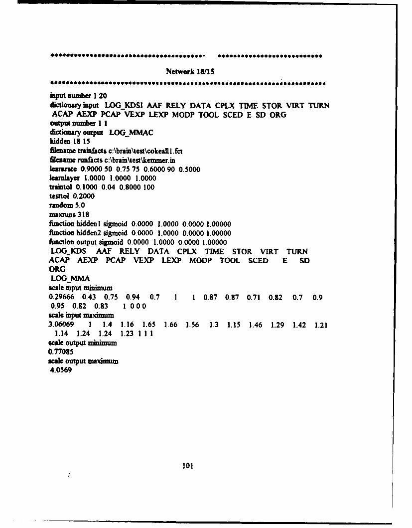
Network 18115
input mnber 1 20dictionary input LOGKDSI AAF RELY DATA CPLX TIME STOR VIRT TURNACAP AEXP PCAP VEXP LEXP MODP TOOL SCED E SD ORGoutput number I Idictionary output LOGQMMAChidden 18 15filename trainfacts c:\brain\test\cokeall l.fctfilename runfacts c:\brain\test\kemmer.mnlearnate 0.9000 50 0.75 75 0.6000 90 0.5000learnlayer 1.0000 1.0000 1.0000traintol 0. 1000 0.04 0.8000 100testtol 0.2000random 5.0maxnms 318fimction hidden I sigmoid 0.0000 1.0000 0.0000 1.00000function hidden2 sigmoid 0.0000 1.0000 0.0000 1.00000function output sigmoid 0.0000 1.0000 0.0000 1.00000LOG KDS AAF RELY DATA CPLX TIME STOR VIRT TURN
ACAP AEXP PCAP VEXP LEXP MODP TOOL SCED E SDORGLOGMMA
scale input minimum0.29666 0.43 0.75 0.94 0.7 1 1 0.87 0.87 0.71 0.82 0.7 0.90.95 0.82 0.83 1 000
scale input maximum3.06069 1 1.4 1.16 1.65 1.66 1.56 1.3 1.15 1.46 1.29 1.42 1.21
1.14 1.24 1.24 1.23 1 11"scale output minimum0.77085scale output maximum4.0569
101
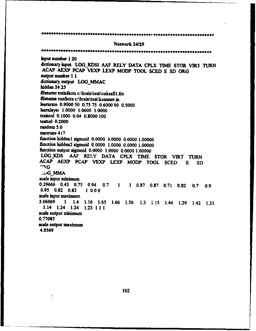
Network 24125
input number 1 20dictionary input LOGKDSI AAF RELY DATA CPLX TIME STOR VIRI TURNACAP AEXP PCAP VEXP LEXP MODP TOOL SCED E SD ORG
output number 11dictionary output LOG MMAChidden 24 25filetame trainftcts c:\brains\test\cokcalll.fctfilesime runfacts c:\brain\test\kmmer.inlearrate 0.9000 50 0.75 75 0.6000 90 0.5000learalayer 1.0000 1.0000 1.0000tritol 0.1000 0.04 0.8000 100temttol 0.2000random 3.0imaxuns 417function hidden I sigmoid 0.0000 1.0000 0.0000 1.00000function hidden2 sigmoid 0.0000 1.0000 0.0000 1.00000function output sigmoid 0.0000 1.0000 0.0000 1.00000LOG KDS AAF RELY DATA CPLX TIME STOR VIRT TURN
ACAP AEXP PCAP VEXP LEXP MODP TOOL SCED E SD
.-;jO MMAscale input minimum0.29666 0.43 0.75 0.94 0.7 1 1 0.87 0.87 0.71 0.82 0.7 0.90.95 0.82 0.83 1 000
scale input maximum3.06069 1 1.4 1.16 1.65 1.66 1.56 1.3 1.15 1.46 1.29 1.42 1.21
1.14 1.24 1.24 1.23 111scale Output minimum0.77085"scale output maximm4.0569
102

Brainmaker Neural Network Training and Testing Files
COCOMO Training and Kemmerer Testing Versions
COKEALLI.FCT
2.03307 1 0.88 1.16 0.7 1 1.06 1.15 1.07 1.19 1.13 1.17 1.11 1.24 1.1 1.04 [ E
3.30963--- 2
2.46686 0.85 0.88 1.16 0.85 1 1.06 1 1.07 1 0.91 1 0.90.95 1.1 1 1 [ E3.20412-32.12057 1 1 1.16 0.85 1 1 0.87 0.94 0.86 0.82 0.86 0.90.95 0.91 0.91 1 [ SD2.3856
-41.77815 0.76 0.75 1.16 0.7 1 1 0.87 1 1.19 0.91 1.42 s0.95 1.24 1 1.04 [ ORG2.38021-51.20412 1 0.88 0.94 1 1 1 0.87 1 1 1 0.86 0.90.95 1.24 1 1 [ ORG1.51851-60.60206 1 0.75 1 0.85 1 1.21 1 1 1.46 1 1.42 0.90.95 1.24 1.1 1 [ ORG1.63346-70.83884 1 0.75 1 1 1 1 0.87 0.87 1 1 1 0.9 0.95
0.91 0.91 1 [ ORG0.90309-81.34242 1 1.15 0.94 1.3 1.66 1.56 1.3 1 0.71 0.91 1 1.211.14 1.1 1.1 1.08 [ E3.0314
-9
103

1.47712 1 1.15 0.94 1.3 1.3 1.21 1.15 1 0.86 1 0.86 1.1
1.07 0.91 1 1 [ E2.62634
-- 101.46239 0.63 1.4 0.94 1.3 1.11 1.56 1 1.07 0.86 0.82 0.86 0.9
1 1 1 1[E2.5065-- 111.50515 0.63 1.4 0.94 1.3 1.11 1.56 1 1.07 0.86 0.82 0.86 0.9
1 1 1 1[E2.33845
-- 121.5682 1 1.15 0.94 1.3 1.11 1.06 1 1 0.86 0.82 0.86 1
0.95 0.91 1 1.08 [ E2.30319
- 13
1.39794 0.96 1.15 0.94 1.3 1.11 1.06 1.15 1 0.71 1 0.7 1.1
1 0.82 1 1IE1.89762-- 140.47712 1 1.15 0.94 1.65 1.3 1.56 1.15 1 0.86 1 0.7 1.1
1.07 1.1 1.24 1.23 [ SD1.86332
-- 150.59106 1 1.4 0.94 1.3 1.3 1.06 1.15 0.87 0.86 1.13 0.86 1.21
1.14 0.91 1 1.23 [ E1.78533--- 16
0.78533 0.6 1.4 1 1.3 1.3 1.56 1 0.87 0.86 1 0.86 1
1 1 1 I [E1.60206
-- 170.5563 0.53 1.4 1 1.3 1.3 1.56 1 0.87 0.86 0.82 0.86 1
1 1 1 1[E0.95424
-- 182.50515 1 1.15 1.16 1.15 1.3 1.21 1 1.07 0.86 1 1 1
1 1.24 1.1 1.08 [ E4.0569-,- 19
3.06069 0.84 1.15 1.08 1 1.11 1.21 0.87 0.94 0.71 0.91 1 1
1 0.91 0.91 1 [ E3.81954
104
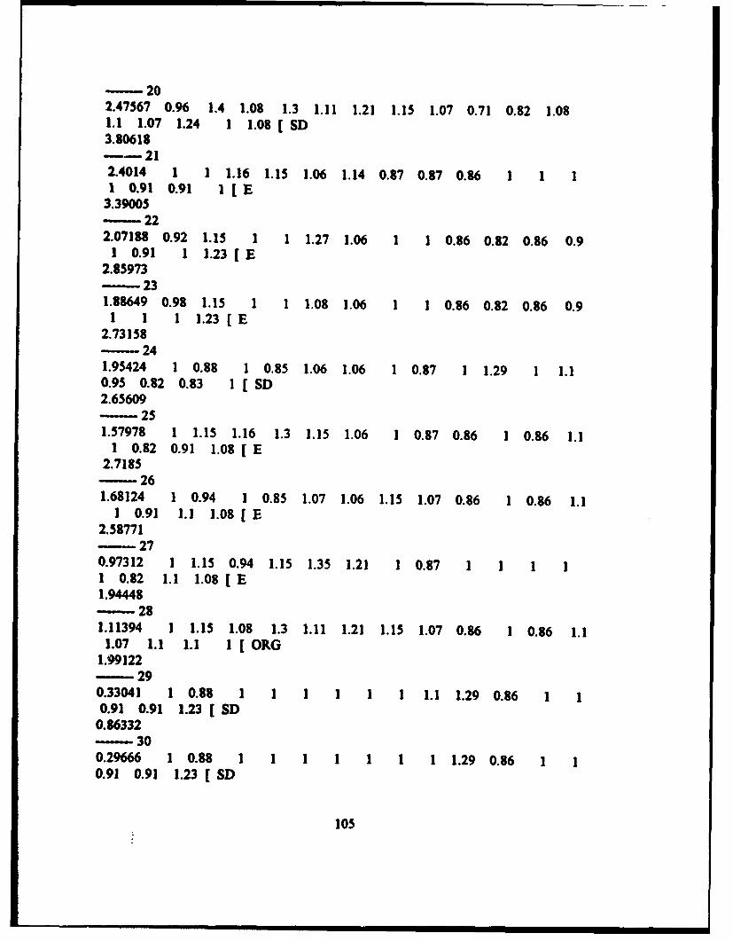
--- 202.47567 0.96 1.4 1.08 1.3 1.11 1.21 1.15 1.07 0.71 0.82 1.081.1 1.07 1.24 1 1.08 [ SD3.80618
-- 212.4014 1 1 1.16 1.15 1.06 1.14 0.87 0.87 0.86 11 0.91 0.91 1 [E
3.39005-- 222.07188 0.92 1.15 1 1 1.27 1.06 1 1 0.86 0.82 0.86 0.9
1 0.91 1 1.23 [E2.85973
--- 231.88649 0.98 1.15 1 1 1.08 1.06 1 1 0.86 0.82 0.86 0.91 1 1 1.23[ E
2.73158-241.95424 1 0.88 1 0.85 1.06 1.06 1 0.87 1 1.29 1 1.10.95 0.82 0.83 1 [ SD2.65609- 251.57978 1 1.15 1.16 1.3 1.15 1.06 1 0.87 0.86 1 0.86 1.1
1 0.82 0.91 1.08 [ E2.7185- 261.68124 1 0.94 1 0.85 1.07 1.06 1.15 1.07 0.86 1 0.86 1.1
1 0.91 1.1 1.08 [ E2.58771- 270.97312 1 1.15 0.94 1.15 1.35 1.21 1 0.87 1 11 0.82 1.1 1.08 [ E1.94448- 281.11394 1 1.15 1.08 1.3 1.11 1.21 1.15 1.07 0.86 1 0.86 1.1
1.07 1.1 1.1 1 [ ORG1.99122- 290.33041 1 0.88 1 1 1 1 1 1 1.1 1.29 0.860.91 0.91 1.23 [ SD
0.86332- 300.29666 1 0.88 1 1 1 1 1 1 1 1.29 0.860.91 0.91 1.23 [ SD
105

0.77085--- 311.79239 0.81 1.4 1.08 1 1.48 1.56 1.15 1.07 0.86 0.82 0.86 1.1
1.07 1 1 1 [ E3.02653
322.59106 0.67 0.88 1.08 0.85 1 1 1 1 0.71 0.82 1 11 1.1 1.1 1 [ SD
2.84633-- 331.62324 0.96 1.4 1.08 1.3 1.48 1.56 1.15 0.94 0.86 0.82 0.860.9 1 0.91 0.91 1 [ E2.78175-- 341.36172 0.96 1.15 1.08 1 1.06 1 1 0.87 1 1 1 1 1
0.91 1.1 1.23 [ E2.36172
-- 351.11394 1 0.75 0.94 1.3 1.06 1.21 1.15 1 1 0.91 1 1.11 1.24 1.24 1 [ E
1.91381-- 361.17609 0.81 0.88 1.08 0.85 1 1 0.87 0.87 1.19 1 1.17 0.90.95 1 0.91 1.04 [ SD1.74036-- 371.77815 0.56 0.88 0.94 0.7 1 1.06 1 1 0.86 0.82 0.86
I I I 1 [ ORG1.67209- 381.17609 1 1 1 1.15 1 1 0.87 0.87 0.71 0.91 1 0.9"A95 0.82 0.91 1 [ ORG1.07918-- 390.79239 1 1 1 1.15 1 1 0.87 1 0.71 0.82 0.7 10.95 0.91 1.1 1 [ ORG0.90309-- 400.47712 0.83 1 0.94 1.3 1 1 1 0.87 0.86 0.82 1.171 1.1 1 1 [ ORG
0.90309-- 41
106
0.72427 1 0.88 0.94 1 1 1 0.87 0.87 1 0.82 0.7 0.90.95 0.91 0.91 1 [ ORG0.77815- 421.65801 0.43 0.88 1.04 1.07 1 1.06 0.87 1.07 0.86 1 0.93 0.9
0.95 0.95 0.95 1.04 [ ORG1.65321-- 431.45636 0.98 1 1.04 1.07 1 1.21 0.87 1.07 0.86 1 1 0.90.95 1 1 1.04 [ ORG1.91907-441.48572 0.98 0.88 1.04 1.07 1.06 1.21 0.87 1.07 1 1 1 0.90.95 1.1 1 1.04 [ ORG1.93951- 451.54406 0.91 0.88 1.04 1.07 1 1.06 0.87 1.07 1 1 1 0.90.95 1 0.95 1.04 [ ORG2.0253
- 461.86332 0.78 0.88 1.04 1.07 1 1.06 0.87 1.07 1 1 0.86 0.90.95 1 1 1.04 [ ORG
2.10037- 471.36172 1 0.75 0.94 1.3 1 1 0.87 0.87 0.71 0.82 0.7 1.11.07 1.1 1 1.04 [ ORG1.5563
- 482.66651 0.67 0.88 0.94 0.85 1 1 0.87 1 1.19 0.91 1.17 0.90.95 1.1 1 1.04 [ SD
3.10448- 491.95904 1 1 1 0.85 1 1 1 0.87 0.71 1 0.7 1.1 10.82 0.91 1 [ SD
2.19312- 501.38021 1 1.15 1 1 1.3 1.21 1 0.87 0.86 1 0.86 1.11 1 1 I[E2.24551-51
I 1 0.88 1 1 1 1 1 1.15 1.19 1 1.42 1 0.951.24 1.1 1.04 [ ORG2.08636
107

-- 320.91381 1 0.88 0.94 0.85 1 1.06 1.15 1 1 1 1 1.1
1.07 1.24 1.1 1 [ ORG1.61278-- 330.72427 1 0.88 0.94 1.15 1.11 1.21 1.3 1 0.71 1 0.7 1.1
1.07 1 1.1 1.08 [ SD1.14612-- 540.64345 1 1 0.94 1 1 1.06 1.15 0.87 1 0.82 1 1
0.95 0.91 1.1 1 [ ORG1.30103-- 350.79934 1 0.88 0.94 0.7 1 1 0.87 0.87 0.86 0.82 1.17 0.9
0.95 1.1 1 1 [ ORG1.25527-- 361.43136 1 1.15 0.94 1.3 1.3 1.21 1 1 0.86 0.91 1 1.1
1.07 1.1 1.1 1.08 [ E2.98136
-571.23044 0.87 1 0.94 1.15 1.11 1.21 1.3 1 1 1 1 1.1
1.07 1.1 1.1 1.23 [ E2.37474
581.39794 1 1.4 0.94 1.3 1.66 1.21 1 1 0.71 0.82 0.7 0.9
0.93 0.91 1 1 [ E2.11394
-. 591.36172 0.9 1 0.94 1.15 1.06 1.06 1 0.87 1 1 1 1
1 0.91 1 1 [ ORG1.84509-- 600.82607 1 1.15 0.94 1.3 1.11 1.06 1 1 0.86 1.13 0.86 1.1
1.07 1.1 1.1 1.08 [ ORG1.75587-- 611.44715 1 1 0.94 1.15 1 1 0.87 0.87 0.86 1 0.86 0.9
1 0.82 1 1 [ ORG1.69897-- 620.95904 1 0.88 0.94 1.3 1.11 1.21 1.15 1 0.78 0.82 0.7 1.21
1.14 0.91 1.24 1 [ SD
108
1.57978ý- 631 1 1 0.94 1.15 1 1 1 0.87 0.71 0.82 0.86 1 1
0.82 1 1 [E1.17609
KEMMERIN
LOGKDS AAF RELY DATA CPLX TIME STOR VIRT TURNACAP AEXP PCAP VEXP LEX]P MODP TOOL SCED SD EORGfacts nm- 1
2.40414 1 1.15 1.08 1.15 1 1.06 0.87 1 0.86 1.13 0.86 11 0.82 0.91 1.02 [ SD
-21.60745 1 1 1 1 1 1 0.87 1 1 1.07 0.86 1 1
1 1 1 [SD-32.65321 1 1 1.16 1 1.3 1.21 0.87 1 0.86 1.13 1 11.03 0.91 1 1 [ E-.-- 42.33122 1 1 1.08 0.92 1 1 0.87 0.93 0.8 0.89 0.85 0.970.95. 1 1 1.02 [ SD-52.65311 1 1 0.94 1 1 1 0.93 0.87 0.78 1.13 0.93 1.11.03 1 0.91 1.07 [ OR.G
- 61.69897 1 1 1.16 1 1.11 1.06 1 0.87 0.86 1.13 0.86 0.950.97 0.91 1 1.23 [ E-71.63346 1 1 1.16 1 1.11 1.06 1 0.87 0.86 1.13 0.7 0.951.07 0.91 1 1.23 [ E- 82.22271 1 1.15 1.16 1 1 1 1 0.93 1 0.95 1 0.950.97 1 1 1.16 [ SD-92.46089 1 1 1.16 1.15 1.11 1.06 0.87 0.87 1 1.13 1.06 1.1
I I 1 1.08 [ E- 10
109
1.59106 1 1 1.16 1 1.11 1 0.93 1.03 0.71 1 0,7 1.11.14 1.05 1 1.23 [ SD-- 112.40517 1 1.16 1 1 1 1 1 1 0.86 1.13 0.86 1
0.86 1 1.23 [ SD12
2.10924 1 1 1.16 1 1 1 0.87 0.87 0.86 1.07 0.86 11.03 1.1 0.95 1.08 [ SD
-132.2079 1 1 1.16 1 1.06 1 0.87 0.87 1.19 1 0.78 1.21
0.97 1.1 1 1.08 [ SD14
2.21695 1 1 1.16 1 1 1 0.87 0.87 0.86 1.21 0.93 1.11.1 0.95 0.91 1.04 [ ORG--- 151.77959 1 1 1 1 1 1 1 0.87 0.71 0.91 0.86 1.11.03 0.91 0.91 1 [ SD
110

APPENDIX F
Genetic Algorithm Fitness Function (fit.c)
(Prior to instantiation of awk Wrapper)
#Anclude <math.h>ruct entry (double effort;double akdsi;double ds; Variable Declarationsint il,i2,i3,i4,i5,i6,i7,i8,i9,ii 0,i11,i12,13,14,il 5;int ie; ,
struct entry table[]SeyDimension Table and Include
include "table.c" Fact File "table.c"
int size - (sizeoftable)/(sizeof struct entry));
double fl(y)register double *y;
double res; Dimension Array of 96 numbers for use
double emm- by the fitness fimction.double exp;static double x[96];register it ij;
for(i =0 ; i < 90; i++) { Constrain cost driver size between 0.5x[i] - y[i]+200; and 2.0. Constrain coefficients andx[ij/= 400.0;x41 * 1.5; exponents between 0.0 and 4.0x4i] - .5;
11

fornin 90; i < 96; i+-4)fxfij y[iJ + 200;X[iJ / 100;
ftb(rt- 0, i-0; i< 42; i+-6)(W I (xiJ< x[i+ I D) res +-1000;i(.' (x[iJ< x[i+2J)) rea +-1000;____________i~l (x ni< 41+3])) mc +100; Penalty fimctions to force GAiftJ (4~i]< x[i+41)) rca +in1000;if(I (411< xri+sJ)) rea +a.1000; to obey rules established byi1(! (xfi+lJ< xli+2J)) res +-1000; Boehm for the first severn cost
if(! (41i+11< 41+4])) re +- 1000; drivers. Comment out ifiV! (xli+1j< xfi+5J)) res +.1000; unconstrained drivers areif(! (x4i+2J< xfi+3J)) res +=I1000;if(! (x[i+2J< 41i+4])) res +-1000; desired.if(! (x[i+2J< xfi+5J)) res +-1000;_______________U(~! (x[i+3]< x[i+4])) res +-1000;ifi! (x[i+3]< x4i+5J)) res +=I000;iii! (x[i+4]< x[i+5J)) res+-1000;
foz(i=42; i< 94; i+6-)(A1! Nxip> x~i+ I D) rcs += 000;_______________Ai! (x[iJ> x4i+2])) res +-1000; Penalty finctions to force GA
W~! (411l> 41i+4])) res +-1l000; to obey rules established by
if~! (41i]> x[1+S])) res +-1000; Boehmn for drivers eight throughiV! (x~i+ I]> x[i+2])) res +-1000;A~! (x[1+1J> x~i+3])) res +-1000; fourteen. comment out if
if(! (41i+1]> xfi+4])) rca +-1000; ucntanddie rW~! (x[1+ Ii> 4~i+SJ)) res +-1000;unosriediesaei~! (x[i+2]> x[1+3J)) rea +-1000; desired.if(! (xfi+21> x[i -4])) rca +- 100o;il(! (41i+21> xli+5J)) res +-1000;AlI (x~i+3]> x~i+4J)) res +-I000;if(! (x[i+3J> 41i+5])) res +-I1000;if(! (41i+4]> x[i+5j)) res+1000;
/0 for(im90; i< 91; i++)(
112
if(! (X[i+ IJ <41~+2])) res +-l1000; penalty functions to force GA
) to obey rules established by
for(i-93; i < 94; i++) {Boeham for coefficients andi~l Wi] > x~i+lJ )res +-IONO; exoet.Comment out ifiW! (x[i] > x4i+2J ))s +-1000O; xnetiV1 (xli-sI1] > x4i+2J)) res +- 1000; unconstrained drivens are
) desired.
for(i -0; i < size; i++.)(/0 get product of cost drivers -goes from 0 to 89.. treat as a 6x1IS amy"/eumm xftable[iJ.ill;emm x[table[iJ.i2 + 6];em P x~tablefi].i3 + 6*2];emm D x[table[iJ34 + 6*3];emm X[table[iJ.iS + 6*4];emin xtable[iJ.i6 + 6*5];emm x[table[iJ.i7 + 606];
e Mm x[tablefi].ig + 6*7J;_________________emm x[table[i].i9 + 6*8]; Bl yei ins esremm 'X[table[iJ.iO + 6*9];Bodtpisfnesmar
umM x[table~i].il 1 + 6* 10J; evaluation. Average relative error iseum X[table~i].i12 + 6011];
Ius x[table[Q].13 + 6*12]; shown.emm *ix[table[ij~i14 + 6*13];910M x[table[i].i 15 + 6*14);summ~ x[table[i].ie+90J; /0 coeff 0/em ~pow(table[i].akdsi, x[table[i].ie+93]); 1* exponent1res +
return realsize; Bold underlined type is GAucsd 1.4 declaration
for the chromosome. Translate as 10 bits perP* GAteval fl 10:200df96 % number, range -200 to 200, 96 numbers total.
113
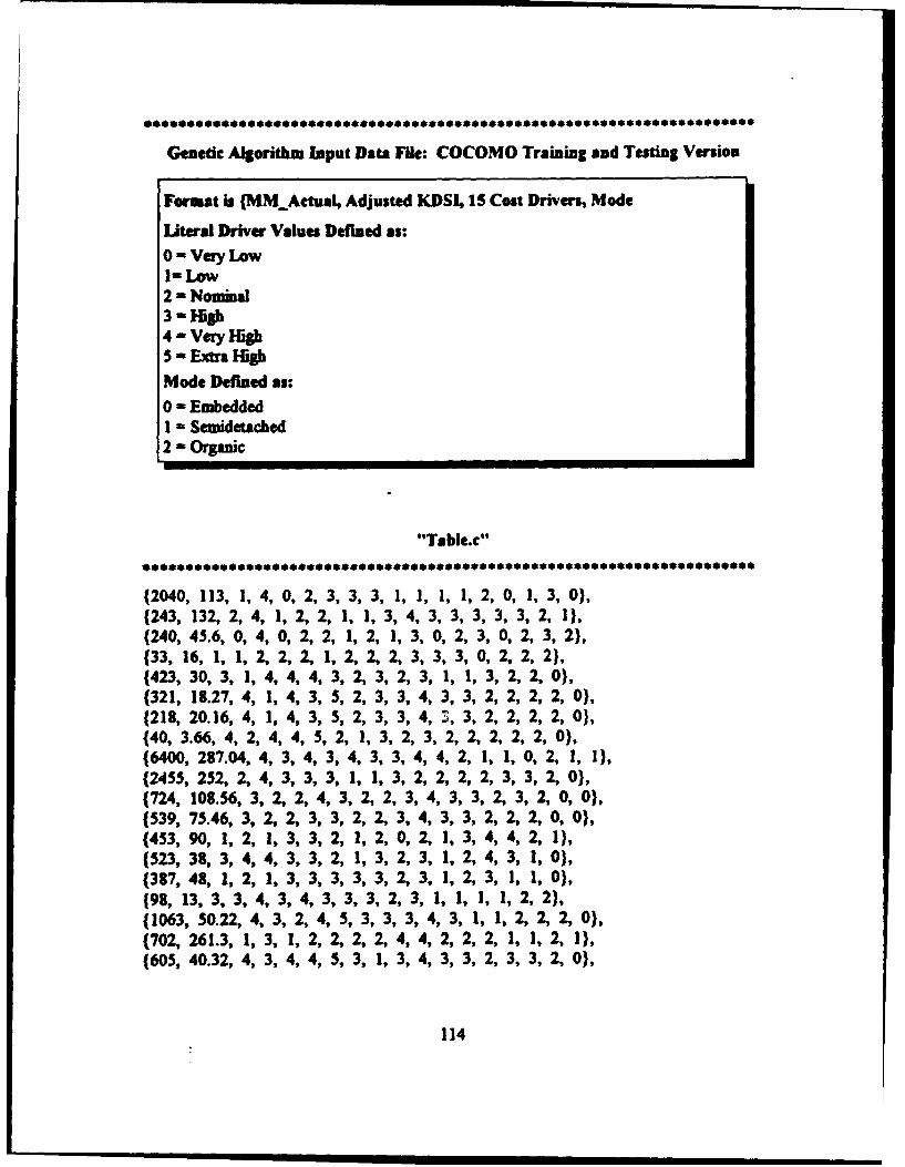
Genetic Algorithm Input Data File: COCOMO Training and Testing Version
Format is (MMActual, Adjusted KDSI, 1S Cost Drivers, Mode
LAteral Driver Values Defined as:
0 - Very LowI- Low2 -Nominal3- High4 Very igh5 Extra HighMode Defined as:
0 - Embedded1 - Semidetached2 - Organic
"Table.c"
(2040, 113, 1, 4, O, 2, 3, 3, 3, ,1, 1, 1, 2, O, 1, 3, 0),(243, 132, 2, 4, 1, 2, 2, 1, 1, 3, 4, 3, 3, 3, 3, 3, 2, 1),(240, 45.6, 0, 4, 0, 2, 2, 1, 2, 1, 3, 0, 2, 3, 0, 2, 3, 2),(33, 16, 1, 1, 2, 2, 2, 1, 2, 2, 2, 3, 3, 3, 0, 2, 2, 2),(423, 30, 3, 1, 4, 4, 4, 3, 2, 3, 2, 3, 1, 1, 3, 2, 2, 0),(321, 18.27, 4, 1, 4, 3, 5, 2, 3, 3, 4, 3, 3, 2, 2, 2, 2, 0),(218, 20.16, 4, 1, 4, 3, 5, 2, 3, 3, 4, T, 3, 2, 2, 2, 2, 0),(40, 3.66, 4, 2, 4, 4, 5, 2, 1, 3, 2, 3, 2, 2, 2, 2, 2, 0),(6400, 287.04, 4, 3, 4, 3, 4, 3, 3, 4, 4, 2, 1, 1, 0, 2, 1, 1),(2455, 252, 2, 4, 3, 3, 3, 1, 1, 3, 2, 2, 2, 2, 3, 3, 2, 0),(724, 108.56, 3, 2, 2, 4, 3, 2, 2, 3, 4, 3, 3, 2, 3, 2, 0, 0),(539, 75.46, 3, 2, 2, 3, 3, 2, 2, 3, 4, 3, 3, 2, 2, 2, 0, 0),(453, 90, 1,2, 1,3,3,2, 1,2,0,2, 1,3,4,4,2, 1),(523, 38, 3, 4, 4, 3, 3, 2, 1, 3, 2, 3, 1, 2, 4, 3, 1, 0),(387, 48, 1, 2, 1, 3, 3, 3, 3, 3, 2, 3, 1, 2, 3, 1, 1, 0),
(98, 13, 3, 3, 4, 3, 4, 3, 3, 3, 2, 3, 1, 1, 1, 1, 2, 2),(1063, 50.22, 4, 3, 2, 4, 5, 3, 3, 3, 4, 3, 1, 1, 2, 2, 2, 0),(702, 261.3, 1, 3, 1, 2, 2, 2, 2, 4, 4, 2, 2, 2, 1, 1, 2, 1),(605, 40.32, 4, 3, 4, 4, 5, 3, 1, 3, 4, 3, 3, 2, 3, 3, 2, 0),
114
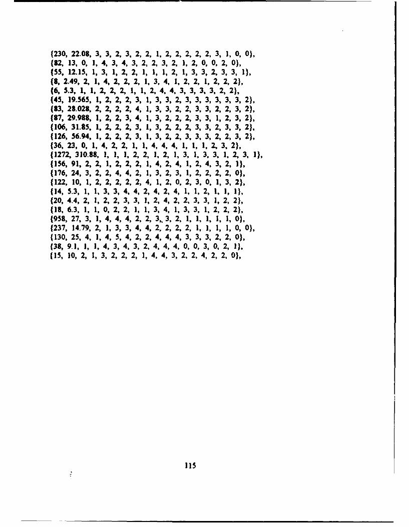
(230, 22.08, 3, 3, 2, 3, 2, 2, 1, 2, 2, 2, 2, 2, 3, 1, 0, 0),(82, 13, 0, 1, 4, 3, 4, 3, 2, 2, 3, 2, 1, 2, 0, 0, 2, 0),(55, 12.15, 1, 3, 1, 2, 2, 1, 1, 1, 2, 1, 3, 3, 2, 3, 3, 1),(8, 2.49, 2, 1, 4, 2, 2, 2, 1, 3, 4, 1, 2, 2, 1, 2, 2, 2),(6, 5.3, 1, 1, 2, 2, 2, 1, 1, 2, 4, 4, 3, 3, 3, 3, 2, 2),(45, 19.565, 1, 2, 2, 2, 3, 1, 3, 3, 2, 3, 3, 3, 3, 3, 3, 2),(83, 28.028, 2, 2, 2, 2, 4, 1, 3, 3, 2, 2, 3, 3, 2, 2, 3, 2),(87, 29.988, 1, 2, 2, 3, 4, 1, 3, 2, 2, 2, 3, 3, 1, 2, 3, 2),(106, 31.85, 1, 2, 2, 2, 3, 1, 3, 2, 2, 2, 3, 3, 2, 3, 3, 2),(126, 56.94, 1, 2, 2, 2, 3, 1, 3, 2, 2, 3, 3, 3, 2, 2, 3, 2),(36, 23, 0, 1, 4, 2, 2, 1, 1, 4, 4, 4, 1, 1, 1, 2, 3, 2),(1272, 310.88, 1, 1, 1, 2, 2, 1, 2, 1, 3, 1, 3, 3, 1, 2, 3, 1),(156, 91, 2, 2, 1,2,2,2, 1,4,2,4, 1,2,4,3,2, 1),(176, 24, 3, 2, 2, 4, 4, 2, 1, 3, 2, 3, 1, 2, 2, 2, 2, 0),(122, 10, 1, 2, 2, 2, 2, 2, 4, 1, 2, 0, 2, 3, 0, 1, 3, 2),(14, 5.3, 1, 1,3,3,4,4,2,4,2,4, 1, 1,2, 1, 1, 1),(20, 4.4, 2, 1, 2, 2, 3, 3, 1, 2, 4, 2, 2, 3, 3, 1, 2, 2),(18, 6.3, 1, 1,0,2,2, 1, 1,3,4, 1,3,3, 1, 2, 2, 2),(958, 27, 3, 1, 4, 4, 4, 2, 2, 3,.3, 2, 1, 1, 1, 1, 1, 0),(237, 14.79, 2, 1, 3, 3, 4, 4, 2, 2, 2, 2, 1, 1, 1, 1, 0, 0),(130, 25, 4, 1, 4, 5, 4, 2, 2, 4, 4, 4, 3, 3, 3, 2, 2, 0),(38,9.1, 1, 1,4, 3,4, 3,2,4,4,4, ,0, 3, 0,2, 1),(15, 10,2, 1,3,2,2,2, 1,4,4, 3,2,2,4, 2,2, 0),
115

APPENDIX G
Genetic Programming Fitness Function File"fitnes.C"
#include <math.h>1*
SGPC: Simple Genetic Programming in C(c) 1993 by Waker Alden Tackett and Aviram Carmi
This code and documentation is copyrighted and is not in the public domain.
All rights reserved.
- This notice may not be removed or altered.
- You may not try to make money by distributing the package or by using theprocess that the code creates.
- You may not distribute modified versions without clearly documenting yourchanges and noti'ng the principal author.
- The origin of this software must not be misrepresented, either byexplicit claim or by omission. Since few users ever read sources,credits must appear in the documentation.
- Altered versions must be plainly marked as such, and must not bemisrepresented as being the original software. Since few users ever readsources, credits must appear in the documentation.
- The authors are not responsible for the consequences of use of thissoftware, no matter how awful, even if they arise from flaws in it.
If you make changes to the code, or have suggestions for changes,let us Imow. ([email protected])0/
#ifadef lint
116
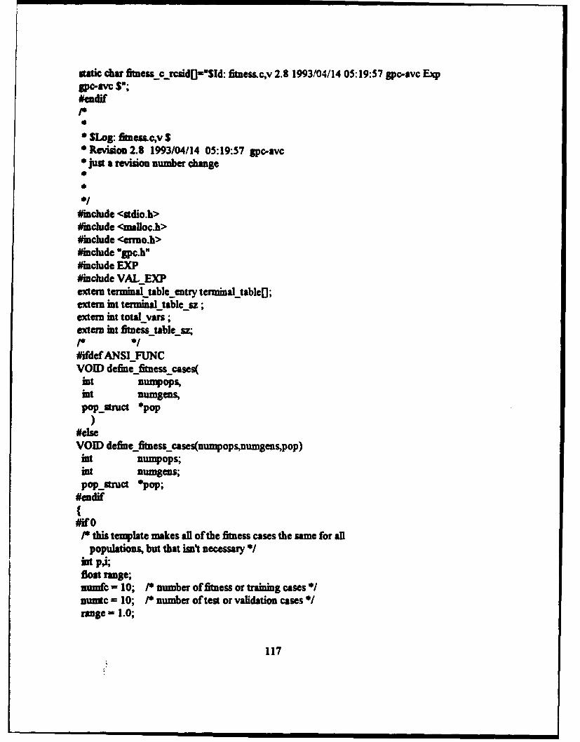
static char fitness•tcrcsid[-"Sld: fitness.cv 2.8 1993/04/14 05:19:57 gpc-avc ExpPC-anc S";
#endif
* SLog: finesLcv S* Revision 2.8 1993/04/14 05:19:57 gpc-avc* just a revision number change
#include <stdio.h>#include <malloc.h>#include <ermo.h>#include "gpc.h"#include EXP#include VAL EXPextern terminal tableentry terminal tableD;exten mt terminal-table sz;extern int total vars ;extern int fitnesstablesz;
#ifdef ANSIFUNCVOID define fitness_cases(ait numpops,int numgens,poputnruct *Pop
)#elseVOID definefitnesscases(numpopsnumgenspop)
int numpops;int numsens;popstruct *pop;
#endif
#if 0/* this template makes all of the fitness cases the same for all
populations, but that isn't necessary /hit pj;float range;numfc - 10; /0 number of fitness or training cases */numtc = 10; /* number of test or validation cases /range 1.0;
117

fltuess -cases table - (Bloat =) maCOc~UMPOPOSiZ0(ltest-cases table -(float **) malloc(Dwnpops sizeooffloat *));fitness casesý table out - (Boat **) malloc(numapops~simC~flost s)test-cases..table out - (float **) mAlloc~sunpops~siZmofflost))for (p-0o; p<numwcps; p4-4) (
fitness-cases tablelpJ - (Bloat 0) malioc(onumfc * sizeoIfloat));ttst -cases tablelp] (float *) malloc(nurntc * sizeof(lOat));hiwess...cases table out[p] - (float *) mslloc(numfc 0 sizeo1gflost));test cases tAb k-outlpJ (float *) malioc(nuwmc 0 sizeflifloat));for (I-mO; iznumfc; i++)(/0 evenly spaced zero..anwge: 0/fitnese. cases, tablelp~il range 0 (flostýi / (Bloat nmC;,* evenly spaced 'Tange' about zero:
fitness; cases tabletpJ[iJ - (2.0*ranges(float)i/(float)nIumfc)-angC,
fitness-cases table -out[pJ[i]regressionfiuntion(fitness...cases .. tblelp][i]);
for (i0-; i~numtc; i++)/* validation test cases same as the training settest cases tablelp][i] - fitness .. cases...tableLp)[i);I va-idation could be random wihi the range:test-cases-tabletpllij random float(range);or range centered about zero:test -cases -table[p][i] - random float(2.Orange)-range;
test -cases *table - ut[p)[iJ = regression flnction(test-cases...tble[PJ[iJ);
#endif10 no processing needed - we've got data!?
#ifdef AlSIFUNCVOiD evaluate ftessoL.fPopulations(
uat JIumpops,im "1n11gens,
popstrlct~pop.Mnt p
#elseVOID evahiate~finess of opulbtiofl5(flumlpopsluumge'poptp)
int NUMPOPS;mnt numgens;
118
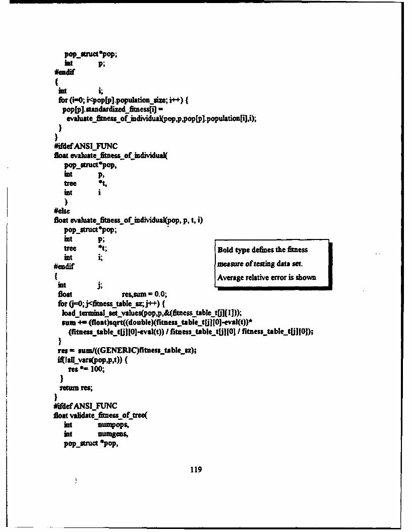
pop Mtruct opop;
#aadif
for (0-0; i<popIpI population size;i+Ipop[jp].standardized htnessfi -
auate-ftessofindividual4op~ppop[p].population[i],i);
#ifdef ANSI FUNCflam valuate-fitness of Mniiul
popatruct~'pop,
tree tint
#ekeBloat evaluate-fitness of individuop p, t, Q)
pop..struct*pop; - ulpp
tree *t;Bold type defines the fitnessint t
#endifmeamure of testing data set.
j; Average relative error is shown
float ressum = 0.0;for Q-=0; j<fitness tablce sz;j++) (load terminal-set values(pop~p,&(flbaessjtablejffl~lJD);sum += (float)sqrt((double)(fitness -table..tUJ 10ievhl(t))*
(rntness...table...tUjI [O-eval(t)) / fitness table-tUl 101/ fitness table tijI 10);
mms sum/((GENERIC)ritnesu..table 2z);
res *= 100;
return res;
#ifdefANSlFUNCfloat validate fitness of tree(
hat numpops,hat nunagens,pop-struct *'Pop,
119

hit ptree O
*elseBoat validate-fttnessý_ofyee(nuinpops, num5Sen, pop, p, t)
int numpops;iat nuagngs;pop-struct *pop;eat Ptree
#Cndzf
intBloat rs, sm - 0.0;float ev;extern mnt vaL fitness table -sz;for (0=0; j<val fitness-table-sz; j++)(
load termnial-set-values(jpop,p,&.(val-fitness..table...t][ 1]));ev - eval(t);sum' 4-m (float)sqrt((double)(valjfitness table tU[0I-ev)*
(vat fitness-table tUl 101-ev) I vai fitness t-able tUl 101Ivai fitness table tjjJ jO);
rums um/((GENERIC)valfitnessjtablejz);ifi~allvYars(Pop'p,t))
)res *= 100; Bold type defines the fitness measure of
retu= res; testing data set. Average relative error
is shown.
#ifdef ANSI FUNCint terminate~early(
int numpops,int nunignspop.struct *Pop
#elseint tcrmnateeacrly(numpops~numgens~pop)
iat nunipops;int numgcns;pop-;ruct *Pop;
#endif
120
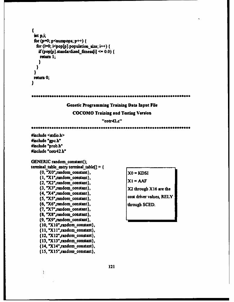
intp'i;for"(in; pcnuqpops; p4-4)(
for (lulO; i<pop[p].population size; i-'4)(if (pop[p].standardizadjhzness~i] <- 0.0)(reur 1;
return 0;
Genetic Programming Training Data Input File
COCOMO Training and Testing Version"tcotr42.c"
#include <stdio.h>#include gSpc.h"#include "prob.h"#include *cotr42.h*
GENERIC random constantO;terminal table-.entry terminal-tableO=(
(0, WX",random constant), XO = KCDSI(1, 'Xl ,random constant), X1- =(2, "X2",random constant),(3, *MX3"ndom-consant), X2 through X 16 are the(4, 'X"Wrsndomn constant), cs rvrvleRL(5, *X3",random constant), Cs rvrvleRL(6, -X6-,radom constant), through SCED.(7, "X7',rndom..constant),(8, "X8",andom constant),(9, "X9",radom constant),(10, OXIO",random constant),(11, "XIIlrandom constant),(12, "X12",random constant),(13, "X13",random constant),,( 14, "X 14",random-constant),(15, "X1S',random-constant),
121

(16, "X16",rdom Constant),(O,FORMATraudom consant),
iat tennkLtab1e..sz -z sioternanltabley)sizcotctrmimtablc..entry)- 1;iat total_van - FITNESS_.HEIGHT;GENERIC fitness tabl.tpFlTNESS.WIDTHJ[FITNESS.HEIGHT] ( (2040.0000,113.0000, 1.0000, 0.8800, 1.1600, 0.7000, 1.0000,
1.0600, 1.1500, 1.0700, 1.1900, 1.1300, 1.1700,1.1000, 1.0000, 1.2400, 1.1000, 1.0400,
(243.0000, 132.0000, 1.0000, 1.0000, 1.1600,0.8500, 1.0000, 1.0000, 0.8700, 0.9400, 0.8600,
0.8200, 0.8600, 0.9000, 0.9500, 0.9100, 0.9100,1.0000, ),
(240.0000, 60.0000, 0.7600, 0.7500, 1.1600,0.7000, 1.0000, 1.0000, 0.8700, 1.0000, 1.1900,
0.9100, 1.4200, 1.0000, 0.9500, 1.2400, 1.0000,1.0400, ),
(33.0000, 16.0000, 1.0000, 0.8800, 0.9400,1.0000, 1.0000, 1.0000, 0.8700, 1.0000, 1.0000,
1.0000, 0.8600, 0.9000, 0.9500, 1.2400, 1.0000,1.0000, ),
(423.0000, 30.0000, 1.0000, 1.1500, 0.9400,1.3000, 1.3000, 1.2100, 1.1500, 1.0000, 0.8600,
1.0000, 0.8600, 1.1000, 1.0700, 0.9100, 1.0000,1.0000, ),
(321.0000, 29.0000, 0.6300, 1.4000, 0.9400,1.3000, 1.1100, 1.5600, 1.0000, 1.0700, 0.8600,0.8200, 0.8600, 0.9000, 1.0000, 1.0000, 1.0000,1.0000, },
(218.0000, 32.0000, 0.6300, 1.4000, 0.9400,1.3000, 1.1100, 1.5600, 1.0000, 1.0700, 0.8600,0.8200, 0.8600, 0.9000, 1.0000, 1.0000, 1.0000,1.0000,),
(40.0000, 6.1000, 0.6000, 1.4000, 1.0000,1.3000, 1.3000, 1.5600, 1.0000, 0.8700, 0.8600,
1.0000, 0.8600, 1.0000, 1.0000, 1.0000, 1.0000,1.0000, ),
(6400.0000, 299.0000, 0.9600, 1.4000, 1.0800,1.3000, 1.1100, 1.2100, 1.1500, 1.0700, 0.7100,0.8200, 1.0800, 1.1000, 1.0700, 1.2400, 1.0000,1.0800, ,
122

(2453.0000, 232.0000, 1.0000, 1.0000, 1.1600,
1.1300, 1.0600, 1.1400, 0.8700, 0.8700, 0.8600,
1.0000, 1.0000, 1.0000, 1.0000, 0.9100, 0.9100,
1.0000, },(724.0000, 118.0000, 0.9200, 1.1500, 1.0000,
1.0000, 1.2700, 1.0600, 1.0000, 1.0000, 0.8600,
0.8200, 0.8600, 0.9000, 1.0000, 0.9100, 1.0000,1.2300, ),
(339.0000, 77.0000, 0.9800, 1.1300, 1.0000,
1.0000, 1.0800, 1.0600, 1.0000, 1.0000, 0.8600,
0.8200, 0.8600, 0.9000, 1.0000, 1.0000, 1.0000,
1.2300, },(433.0000, 90.0000, 1.0000, 0.8800, 1.0000,
0.18500, 1.0600, 1.0600, 1.0000, 0.8700, 1.0000,
1.2900, 1.0000, 1.1000, 0.9500, 0.8200, 0.8300,
!.0000, },(523.0000, 38.0000, 1.0000, 1.1500, 1.1600,
1.3000, 1.1300, 1.0600, 1.0000, 0.8700, 0.8600,
1.0000, 0.8600, 1.1000, 1.0000, 0.8200, 0.9100,1.0800, },
(387.0000, 48.0000, 1.0000, 0.9400, 1.0000,
0.8300, 1.0700, 1.0600, 1.1500, 1.0700, 0.8600,1.0000, 0.8600, 1.1000, 1.0000, 0.9100, 1.1000,
1.0800, },(98.0000, 13.0000, 1.0000, 1.1500, 1.0800,
1.3000, 1.1100, 1.2100, 1.1500, 1.0700, 0.8600,
1.0000, 0.8600, 1.1000, 1.0700, 1.1000, 1.1000,
1.0000, },(1063.0000, 62.0000, 0.8100, 1.4000, 1.0800,
1.0000, 1.4800, 1.5600, 1.1500, 1.0700, 0.8600,
0.8200, 0.8600, 1.1000, 1.0700, 1.0000, 1.0000,
1.0000, ),(702.0000, 390.0000, 0.6700, 0. 8800, 1.0800,
0.8500, 1.0000, 1.0000, 1.0000, 1.0000, 0.7100,0.8200, 1.0000, 1.0000, 1.0000, 1.1000, 1.1000,
1.0000, ),(603.0000, 42.0000, 0.9600, 1.4000, 1.0800,
1.3000, 1.4800, 1.5600, 1.1500, 0.9400, 0.8600,0.8200, 0.8600, 0.9000, 1.0000, 0.9100, 0.9100,
1.0000, ),(230.0000, 23.0000, 0.9600, 1.1500, 1.0800,
1.0000, 1.0600, 1.0000, 1.0000, 0.8700, 1.0000,
123

1.0000, 1.0000, 1.0000, 1.0000, 0.9100, 1.1000,1.2300, ,
(82.0000, 13.0000, 1.0000, 0.7500, 0.9400,1.3000, 1.0600, 1.2100, 1.1500, 1.0000, 1.0000,0.9100, 1.0000, 1.1000, 1.0000, 1.2400, 1.2400,1.0000, ),
(55.0000, 15.0000, 0.8100, 0.8800, 1.0800,0.8500, 1.0000, 1.0000, 0.8700, 0.8700, 1.1900,
1.0000, 1.1700, 0.9000, 0.9500, 1.0000, 0.9100,1.0400, ),
( 8.0000, 3.0000, 0.8300, 1.0000, 0.9400,1.3000, 1.0000, 1.0000, 1.0000, 0.8700, 0.8600,0.8200, 1.1700, 1.0000, 1.0000, 1.1000, 1.0000,1.0000, ),
( 6.0000, 5.3000, 1.0000, 0.8800, 0.9400,1.0000, 1.0000, 1.0000, 0.8700, 0.8700, 1.0000,
0.8200, 0.7000, 0.9000, 0.9500, 0.9100, 0.9100,1.0000, ),
(45.0000, 45.5000, 0.4300, 0.8800, 1.0400,1.0700, 1.0000, 1.0600, 0.8700, 1.0700, 0.8600,
1.0000, 0.9300, 0.9000, 0.9500, 0.9500, 0.9500,1.0400, ),
(83.0000, 28.6000, 0.9800, 1.0000, 1.0400,1.0700, 1.0000, 1.2100, 0.o700, 1.0700, 0.8600,
1.0000, 1.0000, 0.9000, 0.9500, 1.0000, 1.0000,1.0400, ),
(87.0000, 30.6000, 0.9800, 0.8800, 1.0400,1.0700, 1.0600, 1.2100, 0.8700, 1.0700, 1.0000,
1.0000, 1.0000, 0.9000, 0.9500, 1.1000, 1.0000,1.0400, ),
(106.0000, 35.0000, 0.9100, 0.8800, 1.0400,1.0700, 1.0000, 1.0600, 0.8700, 1.0700, 1.0000,
1.0000, 1.0000, 0.9000, 0.9500, 1.0000, 0.9500,1.0400, ),
(126.0000, 73.0000, 0.7800, 0.8800, 1.0400,1.0700, 1.0000, 1.0600, 0.8700, 1.0700, 1.0000,
1.0000, 0.8600, 0.9000, 0.9500, 1.0000, 1.0000,1.0400, ),
( 36.0000, 23.0000, 1.0000, 0.7500, 0.9400,1.3000, 1.0000, 1.0000, 0.8700, 0.8700, 0.7100,0.8200, 0.7000, 1.1000, 1.0700, 1.1000, 1.0000,1.0400, ),
124

(1272.0000, 464.0000, 0.6700, 0.8800, 0.9400,0.8500, 1.0000, 1.0000, 0.8700, 1.0000, 1.1900,
0.9100, 1.1700, 0.9000, 0.9500, 1.1000, 1.0000,1.0400, V ,
(156.0000, 91.0000, 1.0000, 1.0000, 1.0000,0.8500, 1.0000, 1.0000, 1.0000, 0.8700, 0.7100,
1.0000, 0.7000, 1.1000, 1.0000, 0.8200, 0.9100,1.0000, ),
(176.0000, 24.0000, 1.0000, 1.1500, 1.0000,1.0000, 1.3000, 1.2100, 1.0000, 0.8700, 0.8600,
1.0000, 0.8600, 1.1000, 1.0000, 1.0000, 1.0000,1.0000, )
(122.0000, 10.0000, 1.0000, 0.8800, 1.0000,1.0000, 1.0000, 1.0000, 1.0000, 1. 1 500, 1.1900,
1.0000, 1.4200, 1.0000, 0.9500, 1.2400, 1.1000,1.0400, ),
{ 14.0000, 5.3000, 1.0000, 0.8800, 0.9400,1.1500, 1.1100, 1.2100, 1.3000, 1.0000, 0.7100,
1.0000, 0.7000, 1.1000, 1.0700, 1.0000, 1.1000,1.0800, ),
(20.0000, 4.4000, 1.0000, 1.0000, 0.9400,1.0000, 1.0000, 1.0600, 1.1500, 0.8700, 1.0000,0.8200, 1.0000, 1.0000, 0.9500, 0.9100, 1.1000,1.0000, },
(18.0000, 6.3000, 1.0000, 0.8800, 0.9400,0.7000, 1.0000, 1.0000, 0.8700, 0.8700, 0.8600,
0.8200, 1.1700, 0.9000, 0.9500, 1.1000, 1.0000,1.0000, ),
(958.0000, 27.0000, 1.0000, 1.1500, 0.9400,1.3000, 1.3000, 1.2100, 1.0000, 1.0000, 0.8600,0.9100, 1.0000, 1.1000, 1.0700, 1.1000, 1.1000,1.0800, },
(237.0000, 17.0000, 0.8700, 1.0000, 0.9400,1.1500, 1.1100, 1.2100, 1.3000, 1.0000, 1.0000,
1.0000, 1.0000, 1.1000, 1.0700, 1.1000, 1.1000,1.2300, },
(130.0000, 25.0000, 1.0000, 1.4000, 0.9400,1.3000, 1.6600, 1.2100, 1.0000, 1.0000, 0.7100,0.8200, 0.7000, 0.9000, 0.9500, 0.9100, 1.0000,1.0000, ),
(38.0000, 9.1000, 1.0000, 0.8800, 0.9400,1.3000, 1.1100, 1.2100, 1.1500, 1.0000, 0.7800,
125

0.8200, 0.7000, 1.2100, 1.1400, 0.9100, 1.2400,1.0000, },
(15.0000, 30.0000, 1.0000, 1.0000, 0.9400,1.1500, 1.0000, 1.0000, 1.000, 0.8700, 0.7100,0.8200, 0.8600, 1.0000, 1.0000, 0.8200, 1.0000,1.0000, },
Jnt fitness table sz FITNESS WIDTH;GENERIC fitnesstablefFITNESSHEIGHTM[FITNESS WIDTH];
Per Script for Creating Genetic Programming Input Training Data File"derme.pl"
(Author: Ranjan Bagchi)
#!/public/gnu/bin/perl -
# define - generates static data instantiating aU necessary# terminals.
Sfirst - 0;Soutf= SARGV[0];open(OUT,'">Soutf c");open(OUTh,">Soutfh");while(o)
il•/~w*$/){next;
)@1 = upli(, ');
KUSfMr = 0)(print OUT
"#include <stdio.h>\n","#include \*gpc.h\"1zn,"#include \"prob.h\\n"',sprinti"#include \"%s.h\e1n",Soutf),"\nGENERIC random constanto;\n"
print OUT"terminal tablemtry terminal table[ = {\n";
for(0..S#1-1) (
126

prWtOUT %t(%d, \OXO/d\",random-constant),\n",S-,SJ;
puint OUT -vt(O,FORMATrsndom-coMat),n-;print OUT *P;\\
ait terminal table zz - sizeo~terimial table)/uzeo~terminal _table cantty) - 1\*
printf (OUT 'lit total-vars -FITNESSIHEIGHT;\u");Irt (OUT"GENER1C fitness tablect[FITNESS WIDTH[FITNESSYHEIGH1
Sforntat
Si ++;printOUT Stbrnat,@l);
print OUT "int fitness-table-sz = FITNESSWIDTH;\n";print OUT "GENERIC fitness_table[FITNESSHEIGHT][FITNESSWIDTH];";close(OUT);
printf(OUT h "#define FITNESS-HEIGHT %d\n", $#1+l1);printirOUThb "#define FITNESS WIDTH "/odfn", Shirst);printf(OUTj h\nWnextern GENERICfitness table(fITNESS HEIGHT][FITNESS _WID7TH]\n)print1(ZOUT) h \n\nexern GENERICfitness table tjlTrNESS WIDTH][FITNESSHEIGHTj;\n");
close (OUTý h);
Genetic Programming Input Testing Data File
COCOMO Training and Testing Version
"icote2l.c"
#include <stdio.h>#include "gpr..h"#include *prob.h"#include, "valdcoe2lI.h"
127
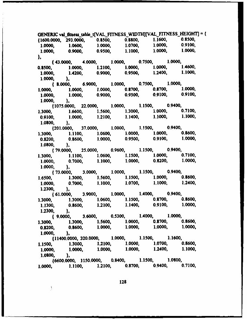
GENERIC valfi-ess table t[VAL_FNESS WIDTMH](VAL FrrNESSHEIGMHT](1600.0000, 293.0000, 0.8500, 0.8800, 1.1600, 0.8500,
1.0000, 1.0600, 1.0000, 1.0700, 1.0000, 0.9100,1.0000, 0.9000, 0.9500, 1.1000, 1.0000, 1.0000,
},(43.0000, 4.0000, 1.0000, 0.7500, 1.0000,
0.8500, 1.0000, 1.2100, 1.0000, 1.0000, 1.4600,1.0000, 1.4200, 0.9000, 0.9500, 1.2400, 1.1000,1.0000,
( 8.0000, 6.9000, 1.0000, 0.7500, 1.0000,1.0000, 1.0000, 1.0000, 0.8700, 0.8700, 1.0000,
1.0000, 1.0000, 0.9000, 0.9500, 0.9100, 0.9100,1.0000,
(1075.0000, 22.0000, 1.0000, 1.1500, 0.9400,1.3000, 1.6600, 1.5600, 1.3000, 1.0000, 0.7100,0.9100, 1.0000, 1.2100, 1.1400, 1.1000, 1.1000,1.0800,
(201.0000, 37.0000, 1.0000, 1.1500, 0.9400,1.3000, 1.1100, 1.0600, 1.0000, 1.0000, 0.8600,0.8200, 0.8600, 1.0000, 0.9500, 0.9100, 1.0000,1.0800,
(79.0000, 25.0000, 0.9600, 1.1500, 0.9400,1.3000, 1.1100, 1.0600, 1.1500, 1.0000, 0.7100,
1.0000, 0.7000, 1.1000, 1.0000, 0.8200, 1.0000,1.0000,
(73.0000, 3.0000, 1.0000, 1.1500, 0.9400,1.6500, 1.3000, 1.5600, 1.1500, 1.0000, 0.8600,
1.0000, 0.7000, 1.1000, 1.0700, 1.1000, 1.2400,1.2300,
(61.0000, 3.9000, 1.0000, 1.4000, 0.9400,1.3000, 1.3000, 1.0600, 1.1500, 0.8700, 0.8600,
1.1300, 0.8600, 1.2100, 1.1400, 0.9100, 1.0000,1.2300,
( 9.0000, 3.6000, 0.5300, 1.4000, 1.0000,1.3000, 1.3000, 1.5600, 1.0000, 0.8700, 0.8600,0.8200, 0.8600, 1.0000, 1.0000, 1.0000, 1.0000,1.0000,
(11400.0000, 320.0000, 1.0000, 1.1500, 1.1600,1.1500, 1.3000, 1.2100, 1.0000, 1.0700, 0.8600,
1.0000, 1.0000, 1.0000, 1.0000, 1.2400, 1.1000,1.0800,
(6600.0000, 1150.0000, 0.8400, 1.1500, 1.0800,1.0000, 1.1100, 1.2100, 0.8700, 0.9400, 0.7100,
128
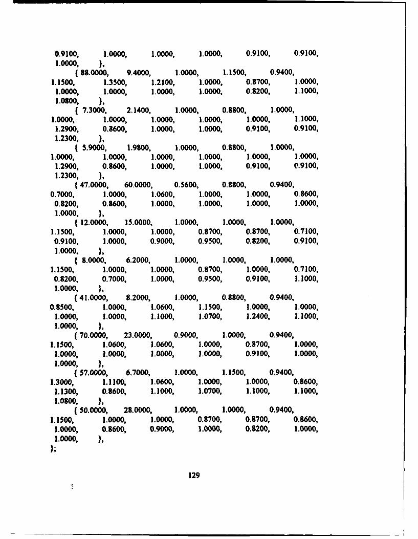
0.9100, 1.0000, 1.0000, 1.0000, 0.9100, 0.9100,1.0000,
(88.0000, 9.4000, 1.0000, 1.1500, 0.9400,1.1500, 1.3500, 1.2100, 1.0000, 0.8700, 1.0000,
1.0000, 1.0000, 1.0000, 1.0000, 0.8200, 1.1000,1.0800,
4 7.3000, 2.1400, 1.0000, 0.8800, 1.0000,1.0000, 1.0000, 1.0000, 1.0000, 1.0000, 1.1000,
1.2900, 0.9600, 1.0000, 1.0000, 0.9100, 0.9100,1.2300,
( 5.9000, 1.9800, 1.0000, 0.8800, 1.0000,1.0000, 1.0000, 1.0000, 1.0000, 1.0000, 1.0000,
1.2900, 0.8600, 1.0000, 1.0000, 0.9100, 0.9100,1.2300,
(47.0000, 60.0000, 0.5600, 0.8800, 0.9400,0.7000, 1.0000, 1.0600, 1.0000, 1.0000, 0.8600,
0.8200, 0.8600, 1.0000, 1.0000, 1.0000, 1.0000,1.0000,
(12.0000, 15.0000, 1.0000, 1.0000, 1.0000,1.1500, 1.0000, 1.0000, 0.8700, 0.8700, 0.7100,0.9100, 1.0000, 0.9000, 0.9500, 0.8200, 0.9100,1.0000,
( 8.0000, 6.2000, 1.0000, 1.0000, 1.0000,1.1500, 1.0000, 1.0000, 0.8700, 1.0000, 0.7100,0.8200, 0.7000, 1.0000, 0.9500, 0.9100, 1.1000,1.0000,
(41.0000, 8.2000, 1.0000, 0.8800, 0.9400,0.8500, 1.0000, 1.0600, 1.1500, 1.0000, 1.0000,
1.0000, 1.0000, 1.1000, 1.0700, 1.2400, 1.1000,1.0000, ),
(70.0000, 23.0000, 0.9000, 1.0000, 0.9400,1.1500, 1.0600, 1.0600, 1.0000, 0.8700, 1.0000,
1.0000, 1.0000, 1.0000, 1.0000, 0.9100, 1.0000,1.0000,
(57.0000, 6.7000, 1.0000, 1.1500, 0.9400,1.3000, 1.1100, 1.0600, 1.0000, 1.0000, 0.8600,
1.1300, 0.8600, 1.1000, 1.0700, 1.1000, 1.1000,1.0800, ),
(50.0000, 28.0000, 1.0000, 1.0000, 0.9400,1.1500, 1.0000, 1.0000, 0.8700, 0.8700, 0.8600,
1.0000, 0.8600, 0.9000, 1.0000, 0.8200, 1.0000,1.0000,
129

int val fitness, table az - VAL FITNESS WIDTH;
GENERIJC val fitness table[VALITNESS ]HEIGHTJ[VALFITNESS WID)TH;
Perl Script for Creating Genetic Programming Input Testing Data File
"val-define.pi"
(Author: Rmnjan Bagchi)
#!/public/gnu/iainperl -
# define - geneantes static data instantiating all necessary# terminals,
Sfirst M0;Soutf = vaI SARGV[0]";open(OUT,ŽSoutf c");open(OUTý_h,*>Soutf h");whll(O>) I
next;
@1 qlk(');dftSfirst -O)
print OUT"#include <stdio.h>\n',"#include \"gpc.h\"\n","#include \"prob.h\*\n",sprintif"#include, \"%s.b\w\n",Soutf),"GENERIC
val fitness table t[VAL _FITNSSWID7hI[VAL _FITNSS HEIGHT]
Sformat=
S OUr T 44; maO
printf(OUT Sfo\nnt@l)
print OUT lint val fitness table-sz - VALFUNESS. WIDTH,~n";print OUT "GENEFRICval fitness, tble[VALIT,_FNESSHEIGHTI[VALFITNESS.WIDTH;w;
130

dose(OUT);
prmt(OUT h "#define VALFITNESS HEIGHT O/d\n, S#W+ );priatf(OUTh "#define VALFTNESS WIDTH %/d\n", Shrst);printOUT h "\n\nextern GENERICval fitness tableVAL-_FITNESS HEIGHT][VALFITNESS._WITH] ;%n);prindrOUTfh "-n\nextern GENEfUCval fitness_tablet[VALFTNESSWIDTH][VALFTNESSHEIGHTj;\n");
close (OUTh);
SGPC Makef'de
COCOMO Training and Testing Phase
## SGPC: Simple Genetic Programming in C## (c) 1993 by Walter Alden Tackett and Aviram Carmi
## This code and documentation is copyrighted and is not in the public domain.
# All rights reserved.
- This notice may not be removed or altered.##
- You may not try to make money by distributing the package or by using the# process that the code creates.
## - You may not distribute modified versions without clearly documenting your## changes and notifying the principal author.
## - The origin of this software must not be misrepresented, either by## explicit claim or by omission. Since few users ever read sources,## credits must appear in the documentation.##
## - Altered versions must be plainly marked as such, and must not be## misrepresented as being the original software. Since few users ever read## sources, credits must appear in the documentation.
## - The authors are not responsible for the consequences of use of this##software, no matter how awflzl, even if they arise from flaws in it.
131

## If you make changes to the code, or have suggestions for changes,0 let us know! ([email protected])
# SId: Makeflleyv 1.1 1993/04/30 05:01:48 gpc-ave Exp gpc-avc S#
# invoke this Makefle with the command: make [ TYPE-type
# where you have the problem-specific fitness and setup files named# fitnessc and setup.c
# TYPE should usually equal int or float, but in principle can be anything.## SLog: Makefile,v S#Revision 1.1 1993/04/30 05:01:48 gpc-avc# Initial revision
# Revisio, 1 7 1993/04/23 01:56:25 gpc-avc
TYPE = floatDEBUG = 0EXP w co'42VALEX - val cote21FLAGS - -0 -DTYPE=S(TYPE) -DDEBUG=S(DEBUG)-DVALEXP"'S(VALrEXP).hV' -DEXP-"$S(EXP).b\"
SRCS = setup.c fitness.c S(EXP).c main.c S(VALEXP).cINCS prob.hOBJS - S(SRCS:%.c=%.o)EXE - Spc- I S(PROBLEM) Bold type indicates problem specific
## NOTE: last definition wins ## declarations that include the COCOMOCC = ace training and testing files created by
CFLAGS - -g -L./lib define.pl and valdefine.pl#CFLAGS = -O -l./hJb
CPPFLAGS = S(FLAGS)LIBS -L../hb -IgpcS(TYPE) -hn
132
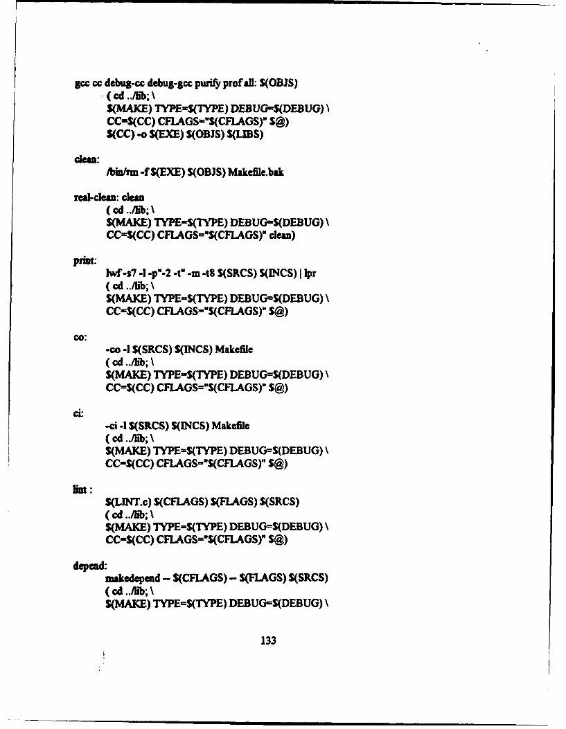
Scc cc debug-cc debug-goc purify, prof all: S(OBJS)
S(MAKE) TYPE=S(TYPE) DEBUGmS(DEBUG)~CC-S(CC) CFIAGS="S(CFIAGS~w S@)S(CC) -o S(EXE) S(OBJS) S(LJBS)
clean:/bin/rm -f S(EXE) S(OBJS) Makefile~bak
real-dlean: clean
S(MAKE) TYPE=-S(TV'PE) DEBUG'=S(DEBUG)\CC=S(CC) CFLAGS="S(CFJ.AGS)" clean)
puint:lW-17 -1 -p"-2 -t" -m -tS S(SRCS) S(INCS) I lpr( cd../hb; \$(MAKE) TYPE=S(TYPE) DEBUG=S(DEBUG)\CC=S(CC) CFLAGS=-S(CFIAGS)" S@)
co:-co -1 S(SRCS) SQINCS) Makefile
S(MAKE) TYPE=$(TYPE) DEBUG=S(DEBUG)\CC=S(CC) CFLAGS="S(CFLAGS)" S@
i -ci -4 S(SRCS) S(INCS) Makefile( cd../Jib; \S(MAKE) TYPE-S(TYPE) DEBUG--S(DEBUG)\CC=S(CC) CFLAGS="S(CFLAGS)" S@)
fiat:S(LINT.c) S(CFLAGS) S(FLAGS) S(SRCS)( cd..Ab; \S(MAKE) TYPE=S(TYPE) DEBUG=S(DEBUG)\CC-$(CC) CFLAGS="S(CFLAGS)" S@)
depend:makedepend - S(CFLAGS) - S(FLAGS) S(SRCS)( cd./hib; \S(MAKE) TYPE=S(TYPE) DEBUG=S(DEBUG)\
133
CC-S(CC) CFLAGS-uS(CFLAGS) S@)
WDO NOT DELETE THIS LINE - make depend depends on it.
"seu.o: /Iw/nclude/stdio.h .Jlib/gPc.h ..Jlb/proto.h..JIhblradolmh"aeu.o: prob.h&utnsso: Aasr/Anchadc/stdio.h /usrfmclude/mafloc.h /usrrmchzde/ernao-hfitness.o: /usrmclude/s~rrNao.h .Jlib/g~pc.h ../hb/protoIifdoess.o: .J.i'b/ran~dom~h
134
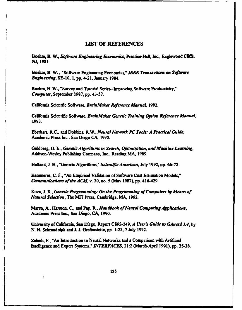
LIST OF REFERENCES
Boehm% B. W., Sofftware Engineering Economics, Prentice-HAl Inc., Englewood Cliffs,NJ, 1981.
Boehm, B. W. , "Software Engineering Economics,' IEEE Transactions on SoftwreEngieering, SE-1O, 1, pp. 4-21, January 1984.
Boehm,6 B. W.11"Survey and Tutorial Series-Improving Software Productivity,'Computer, September 1987, pp. 43-57.
California Scientfic Software, BrainMaker Reference Manual, 1992.
California Scientific Software, BrainMaker Genetic Training Option Reference Manual,1993.
Eberhart, R. C., and Dobbins, R.W., Neu ral Netwok PC Tools: A Practical Guide,Academic Press Inc., San Diego CA, 1990.
Goldberg, D. E., Genetic Algorithms in Search, Optimization, and Machine Learning,Addison-Wesley Publishing Comapany, Inc., Reading MA, 1989.
Holland, J. H., 'Genetic Algorithms," Scientific American, July 1992, pp. 66-72.
Kemmerer, C. F., "An Empirical Validation of Software Cost Estimnation Models,Communications of the ACM, v. 30, no. 5 (May 1987), pp. 416-429.
Koza, J. R., Genetic Programming:- On the Programming of Computers by Means ofNatural Selection, The MIT Press, Cambridge, MA, 1992.
Maren, A., Hurston, C., and Pap, R., Handbook of Neural Computing Applications,Academic Press Inc., San Diego, CA, 1990.
University of California, San Diego, Report CS92-249, A User's Guide to GAucsd 1.4, byN. N. Schraudolph and J. J. Grefenstette, pp. 1-23, 7 July 1992.
Zahedi F., "An Introduction to Neural Networks and a Comparison with ArtificialIntelligence and Expert Systems,* INTERFACES, 21:2 (March-April 1991), pp. 25-38.
135
INITIAL DISTRIBUTION LIST
1. Defense Technical Information Center 2Cameron StationAlexandria, VA 22304-6145
2. Lbrary, Code 52 2Naval Postgraduate SchoolMonterey, CA 93943-5002
3. Dr. Balasubramanium Ramesh, Code AS/RA 5Department of Administrative SciencesNaval Postgraduate SchoolMonterey, CA 93943-5000
4. Dr. Tarek K Abdel-Hamid, Code AS/AH 2Department of Administrative SciencesNaval Postgraduate SchoolMonterey, CA 93943-5000
5. LT Michael A. Kelly 31216 Sylvan Rd.Roanoke, VA 24014
136