DS-15-1379: Virtual Vehicle Control Concept forHydrostatic Dynamometer Control ⇤†

Zhekang Du, Tan Cheng, Perry Y. Li, Kai Loon Cheong and Thomas R. ChaseCenter of Compact and Efficient Fluid Power

Department of Mechanical EngineeringUniversity of MinnesotaMinneapolis, MN 55455.

Email: {duxxx139,cheng164, lixxx099, cheo0013, trchase}@umn.edu.Please send all correspondence to Perry Y. Li.

ABSTRACTAn approach for controlling a hydrostatic dynamometer for the Hardware-In-the-Loop (HIL) testing of hybrid

vehicles is proposed and experimentally evaluated. The hydrostatic dynamometer, which is capable of absorbingand regenerating power, was specifically designed and built in-house to evaluate the fuel economy and controlstrategy of a hydraulic hybrid vehicle being developed. Unlike a chassis dynamometer whose inertia is similarto the inertia of the vehicle being tested, the inertia of this hydro-static dynamometer is only 3% of the actualvehicle. While this makes the system low cost, compact and flexible for testing vehicles with different weightsand drag characteristics, control challenges result. In particular, the dynamometer must apply, in addition to thetorques to mimic the wind and road drag, also the torques to mimic the acceleration and deceleration of the missinginertia. To avoid estimating the acceleration and deceleration, which would be a non-causal operation, a virtualvehicle concept is introduced. The virtual vehicle model generates, in response to the applied vehicle torque, areference speed profile which represents the behavior of the actual vehicle if driven on the road. This reformulatesthe dynamometer control problem into one of enabling the actual vehicle-dynamometer shaft to track the speed ofthe virtual vehicle, instead of directly applying a desired torque. To track the virtual vehicle speed, a controllerwith feedforward and feedback components is designed using an experimentally validated dynamic model of thedynamometer. The approach has been successfully tested on a power-split hydraulic hybrid vehicle with acceptablevirtual vehicle speed and dynamometer torque tracking performance.

1 Introduction

Hardware-In-the-Loop (HIL) simulation is an efficient technique to develop and test complex real-time embedded sys-tems. A HIL system reduces testing complexity by using only part of the hardware which needs to be tested, while theremaining hardware is simulated on the computer. HIL is widely used in the automotive industry to verify the performanceof production powertrain controller modules (PCM) [1].

A prototype hydraulic hybrid passenger vehicle test-bed is being developed within the Center for Compact and EfficientFluid Power (CCEFP) to advance hydraulic hybrid technologies. While simulations can predict fuel economy and perfor-mance of the vehicle, experimental validation is still necessary. Outdoor road tests require a test track and results may not berepeatable due to variable environmental conditions such as wind, rain, snow, and road and traffic conditions. A reliable HILsystem, such as a dynamometer (or dyno in short), can enable reliable and consistent measurements in the laboratory and notbe influenced by environmental factors. Furthermore, a dynamometer allows the comparison, development, and tuning ofvarious control strategies for different vehicle characteristics and driving conditions. To this end, a hydrostatic dynamometercapable of both absorbing and regenerating energy (a necessity for testing hybrid vehicles) has recently been developed inour group [2].

⇤To appear in the ASME Journal of Dynamic Systems Measurement and Control. Original submission: August 16, 2015. Revised: May 23, 2016 andJuly 20, 2016

†A preliminary version of this paper was presented at the 2014 ASME Dynamic Systems and Control Conference, San Antonio, TX.

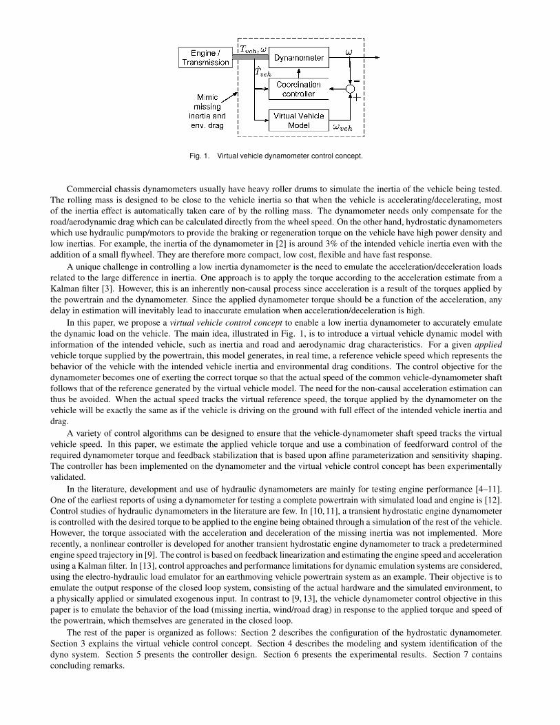
Fig. 1. Virtual vehicle dynamometer control concept.

Commercial chassis dynamometers usually have heavy roller drums to simulate the inertia of the vehicle being tested.The rolling mass is designed to be close to the vehicle inertia so that when the vehicle is accelerating/decelerating, mostof the inertia effect is automatically taken care of by the rolling mass. The dynamometer needs only compensate for theroad/aerodynamic drag which can be calculated directly from the wheel speed. On the other hand, hydrostatic dynamometerswhich use hydraulic pump/motors to provide the braking or regeneration torque on the vehicle have high power density andlow inertias. For example, the inertia of the dynamometer in [2] is around 3% of the intended vehicle inertia even with theaddition of a small flywheel. They are therefore more compact, low cost, flexible and have fast response.

A unique challenge in controlling a low inertia dynamometer is the need to emulate the acceleration/deceleration loadsrelated to the large difference in inertia. One approach is to apply the torque according to the acceleration estimate from aKalman filter [3]. However, this is an inherently non-causal process since acceleration is a result of the torques applied bythe powertrain and the dynamometer. Since the applied dynamometer torque should be a function of the acceleration, anydelay in estimation will inevitably lead to inaccurate emulation when acceleration/deceleration is high.

In this paper, we propose a virtual vehicle control concept to enable a low inertia dynamometer to accurately emulatethe dynamic load on the vehicle. The main idea, illustrated in Fig. 1, is to introduce a virtual vehicle dynamic model withinformation of the intended vehicle, such as inertia and road and aerodynamic drag characteristics. For a given appliedvehicle torque supplied by the powertrain, this model generates, in real time, a reference vehicle speed which represents thebehavior of the vehicle with the intended vehicle inertia and environmental drag conditions. The control objective for thedynamometer becomes one of exerting the correct torque so that the actual speed of the common vehicle-dynamometer shaftfollows that of the reference generated by the virtual vehicle model. The need for the non-causal acceleration estimation canthus be avoided. When the actual speed tracks the virtual reference speed, the torque applied by the dynamometer on thevehicle will be exactly the same as if the vehicle is driving on the ground with full effect of the intended vehicle inertia anddrag.

A variety of control algorithms can be designed to ensure that the vehicle-dynamometer shaft speed tracks the virtualvehicle speed. In this paper, we estimate the applied vehicle torque and use a combination of feedforward control of therequired dynamometer torque and feedback stabilization that is based upon affine parameterization and sensitivity shaping.The controller has been implemented on the dynamometer and the virtual vehicle control concept has been experimentallyvalidated.

In the literature, development and use of hydraulic dynamometers are mainly for testing engine performance [4–11].One of the earliest reports of using a dynamometer for testing a complete powertrain with simulated load and engine is [12].Control studies of hydraulic dynamometers in the literature are few. In [10, 11], a transient hydrostatic engine dynamometeris controlled with the desired torque to be applied to the engine being obtained through a simulation of the rest of the vehicle.However, the torque associated with the acceleration and deceleration of the missing inertia was not implemented. Morerecently, a nonlinear controller is developed for another transient hydrostatic engine dynamometer to track a predeterminedengine speed trajectory in [9]. The control is based on feedback linearization and estimating the engine speed and accelerationusing a Kalman filter. In [13], control approaches and performance limitations for dynamic emulation systems are considered,using the electro-hydraulic load emulator for an earthmoving vehicle powertrain system as an example. Their objective is toemulate the output response of the closed loop system, consisting of the actual hardware and the simulated environment, toa physically applied or simulated exogenous input. In contrast to [9, 13], the vehicle dynamometer control objective in thispaper is to emulate the behavior of the load (missing inertia, wind/road drag) in response to the applied torque and speed ofthe powertrain, which themselves are generated in the closed loop.

The rest of the paper is organized as follows: Section 2 describes the configuration of the hydrostatic dynamometer.Section 3 explains the virtual vehicle control concept. Section 4 describes the modeling and system identification of thedyno system. Section 5 presents the controller design. Section 6 presents the experimental results. Section 7 containsconcluding remarks.

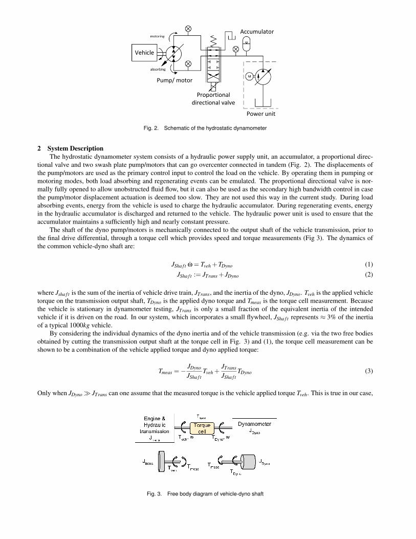
Fig. 2. Schematic of the hydrostatic dynamometer

2 System Description

The hydrostatic dynamometer system consists of a hydraulic power supply unit, an accumulator, a proportional direc-tional valve and two swash plate pump/motors that can go overcenter connected in tandem (Fig. 2). The displacements ofthe pump/motors are used as the primary control input to control the load on the vehicle. By operating them in pumping ormotoring modes, both load absorbing and regenerating events can be emulated. The proportional directional valve is nor-mally fully opened to allow unobstructed fluid flow, but it can also be used as the secondary high bandwidth control in casethe pump/motor displacement actuation is deemed too slow. They are not used this way in the current study. During loadabsorbing events, energy from the vehicle is used to charge the hydraulic accumulator. During regenerating events, energyin the hydraulic accumulator is discharged and returned to the vehicle. The hydraulic power unit is used to ensure that theaccumulator maintains a sufficiently high and nearly constant pressure.

The shaft of the dyno pump/motors is mechanically connected to the output shaft of the vehicle transmission, prior tothe final drive differential, through a torque cell which provides speed and torque measurements (Fig 3). The dynamics ofthe common vehicle-dyno shaft are:

JSha f t w = Tveh +TDyno (1)JSha f t := JTrans + JDyno (2)

where Jsha f t is the sum of the inertia of vehicle drive train, JTrans, and the inertia of the dyno, JDyno. Tveh is the applied vehicletorque on the transmission output shaft, TDyno is the applied dyno torque and Tmeas is the torque cell measurement. Becausethe vehicle is stationary in dynamometer testing, JTrans is only a small fraction of the equivalent inertia of the intendedvehicle if it is driven on the road. In our system, which incorporates a small flywheel, JSha f t represents ⇡ 3% of the inertiaof a typical 1000kg vehicle.

By considering the individual dynamics of the dyno inertia and of the vehicle transmission (e.g. via the two free bodiesobtained by cutting the transmission output shaft at the torque cell in Fig. 3) and (1), the torque cell measurement can beshown to be a combination of the vehicle applied torque and dyno applied torque:

Tmeas =�JDyno

JSha f tTveh +

JTrans

JSha f tTDyno (3)

Only when JDyno � JTrans can one assume that the measured torque is the vehicle applied torque Tveh. This is true in our case,

Fig. 3. Free body diagram of vehicle-dyno shaft

since the dynamometer has been augmented with a small flywheel so that JDyno = 0.2436 kg-m2, JTrans = 0.0064 kg-m2 andJsha f t = 0.25 kg-m2.

3 “Virtual Vehicle” dynamometer control concept

To introduce the “virtual vehicle” control concept, the dynamics of the virtual vehicle are first defined in Section 3.1,and the error attributed to the non-causal acceleration effects is illustrated. The method for modifying the control scheme toavoid the non-causal error is described in Section 3.2.

3.1 Virtual Vehicle dynamics

The virtual vehicle dynamics mimic the behavior of the intended vehicle to be tested given the applied vehicle torque.This includes the inertial dynamics as well as any aerodynamic and road drag. In terms of translational vehicle speed v, theyare:

Mveh v = Fveh �Fdrag(v) (4)

where Mveh is the mass of the vehicle, Fdrag(v) is the road and wind drag, and Fveh is the applied traction force. Note thatMveh and Fdrag(v) need not correspond to the actual vehicle but can be defined arbitrarily for testing vehicles with differentweights, aerodynamic and tire/road characteristics.

Eq.(4) is converted to the rotational domain in terms of the rotation speed of the transmission output shaft

wveh = (rd/Rw) · v

where rd and Rw are the ratio of the output differential gear and the wheel radius, so that:

Jveh wveh = Tveh �Tdrag(wveh) (5)

where Jveh, Tveh and Tdrag are the equivalent vehicle inertia, vehicle torque, and vehicle drag with respect to the transmissionoutput port:

Jveh := MvehR2

w

r2d

Tveh :=Rw

rdFveh

Tdrag(wveh) :=Rw

rdFdrag(v)

In order for the dynamometer to emulate on-the-road driving, from Eqs. (1) and (5), the dynamometer should apply, on thevehicle output shaft, the load of:

TDyno =�(Jveh � JSha f t)wveh �Tdrag(wveh) (6)

where the first term corresponds to the difference in inertia, and the second term corresponds to aerodynamic and road drag.Note that direct implementation of (6) is not strictly possible since the measurement or estimation of the acceleration wveh isnon-causal. Specifically, the acceleration is dependent on the control TDyno applied to it in (1).

Example: To estimate wveh causally, a delay or a causal “dirty differentiator” such as staccs+1 , where tacc is the filter time

constant, is often needed. To see its effect, we assume linear dynamics for simplicity and suppose that the virtual (target)vehicle dynamics are:

Mvehv+bvehv = Fveh (7)

Time - [s]0 2 4 6 8 10

Sp

eed

[m

/s]

0

10

20

30

40

50

60

Test stand speedTarget vehicle speed

Time - [s]0 2 4 6 8 10

Forc

e [N

]

×104

-5

-4

-3

-2

-1

0

1

2

3

4

5

Dyno forceIdeal dyno forceVehicle force

Fig. 4. Speeds (top) and torques (bottom) if the acceleration estimation approach is used for the example.

while the actual test vehicle-dynamometer dynamics are:

Mtest vtest = Fveh +Fdyno (8)

Let the dyno force be defined by:

Fdyno := (Mveh �Mtest) ˆvtest �bvehvtest

where ˆvtest is obtained using the “dirty differentiator” on vtest with some measurement noise. In this example, suppose thatMveh = 20Mtest = 1000kg, bveh = 20N/(m/s), tacc = 1s (to emphasize the effect) and that the vehicle force Fveh is commandedby a driver simulated to be a P-I controller tracking a 3 rad/s sinusoidal drive cycle. Figure 4 shows that the virtual (target)vehicle speed v(t) differs from the test vehicle-dyno speed vtest(t). The applied dyno force also differs significantly from theideal dyno force (i.e. that with vtest obtained (perfectly) from post-processing). This dynamometer control will (most likely)lead to overly optimistic fuel economy results. ⇧

3.2 Control Concept

Given a measurement or estimate of the applied vehicle torque Tveh, the expected transmission output shaft speed profilewveh(t) can be computed in real time by integrating:

Jveh wveh = Tveh �Tdrag(wveh) (9)

Eq.(9) is referred to as the “virtual vehicle” model, and wveh as the “virtual vehicle” (shaft) speed.To avoid the non-causal operation of estimating the acceleration as in [3] or the “dirty differentiator” in the example,

instead of implementing Eq.(6) directly, the dynamometer will control the actual combined dyno-vehicle shaft dynamics (win Eq.(1)) according to the virtual vehicle speed (wveh) (computed in real time based on the measurement or an estimate ofthe applied vehicle torque Tveh and the virtual vehicle dynamics in Eq.(9)).

Suppose that the estimate of the vehicle torque Tveh is accurate, and indeed we are successful in making w(t)! wveh(t),then comparing Eqs.(1) and (5), the dynamometer torque would be:

TDyno =�Jsha f t

JvehTdrag(w)�

Jveh � JSha f t

JvehTveh (10)

Time - [s]0 2 4 6 8 10

Sp

eed

[m

/s]

0

10

20

30

40

50

60

Test stand speedTarget vehicle speed

Time - [s]0 2 4 6 8 10

Forc

e [N

]

×104

-5

-4

-3

-2

-1

0

1

2

3

4

5

Dyno forceIdeal dyno forceVehicle force

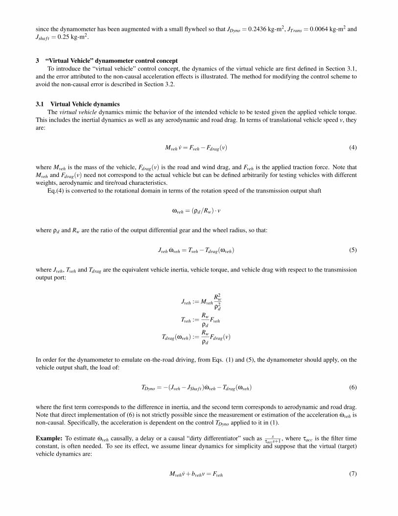
Fig. 5. Speeds (top) and torques (bottom) if the virtual vehicle approach is used

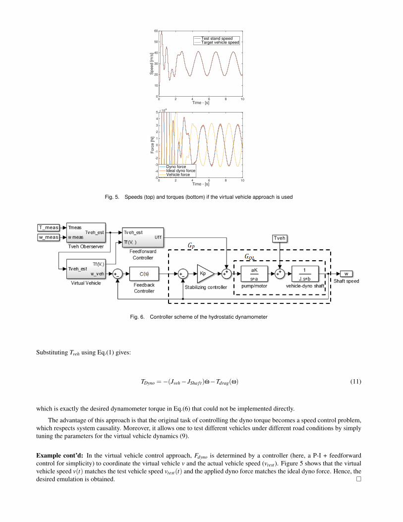
Fig. 6. Controller scheme of the hydrostatic dynamometer

Substituting Tveh using Eq.(1) gives:

TDyno =�(Jveh � JSha f t)w�Tdrag(w) (11)

which is exactly the desired dynamometer torque in Eq.(6) that could not be implemented directly.

The advantage of this approach is that the original task of controlling the dyno torque becomes a speed control problem,which respects system causality. Moreover, it allows one to test different vehicles under different road conditions by simplytuning the parameters for the virtual vehicle dynamics (9).

Example cont’d: In the virtual vehicle control approach, Fdyno is determined by a controller (here, a P-I + feedforwardcontrol for simplicity) to coordinate the virtual vehicle v and the actual vehicle speed (vtest ). Figure 5 shows that the virtualvehicle speed v(t) matches the test vehicle speed vtest(t) and the applied dyno force matches the ideal dyno force. Hence, thedesired emulation is obtained. ⇤

4 Modeling and Identification of the Dynamometer Dynamics

The dyno torque consists of the viscous damping and the pump/motor torque. The pump/motor displacement dynamicsare assumed to be first order. Thus,

TDyno =�b w+Tpm

Tpm(t) = hDP2p

D(t) =

hDP2p

Dmax

�

| {z }K

as+a

[U(·)] (12)

where DP is the system pressure which is regulated to be constant at 19.3 MPa (2800 psi), D(t) is the actual displacementof the pump/motor, Dmax = 56 cc is the maximum displacement of the pump/motor, a is the bandwidth of the swashplatedynamics, b is the damping coefficient, U 2 [0,1] is the normalized displacement command input, and h is the pump/motor’smean mechanical efficiency.

Thus, the dynamics of the common vehicle-dyno shaft in (1) becomes:

Jsha f t w =�b w+Tveh +K ·U(t) (13)

where K = hDPDmax/(2p). The combined inertia of the vehicle drive train and dyno was estimated from CAD models andengine specifications to be Jsha f t = 0.25 kg-m2.

Combining Eqs.(1) and (12), the open loop transfer function from the pump/motor command U(s) to the shaft speedw(s) (see Fig.6) is:

GOL(s) =w(s)U(s)

=a ·K/Jsha f t

(s+a)(s+b/Jsha f t)(14)

In order to validate the structure of GOL(s) in (14) and to identify the unknown parameters a, b and K, system identifi-cation experiments have been performed. Because of the small physical damping b, an inner closed loop is formed with asmall proportional feedback gain of Kp = 0.01 and with Tveh = 0 to form a closed loop system (Fig. 6):

Gp(s) =KpGOL(s)

1+KpGOL(s)(15)

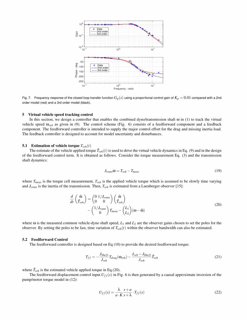
System identification is then performed on Gp(s) by applying a series of sinusoidal reference speeds and measuring its gainsand phases. The model parameters in (14) are optimized to match the measured gains and phases. This way, a second orderclosed loop transfer function was identified to be (Fig. 7):

Gp,2nd(s) =8.28

s2 +2.9s+9.2(16)

The unwrapped open loop system from Gp(s) is:

GOL(s) =828

(s+2.539)(s+0.3574)(17)

This corresponds to a swash-plate bandwidth of a = 2.539 rad/s, damping coefficient of b = 0.3574rad/s⇥Jsha f t = 0.0893Nm/(rad/s), K = 81.5 Nm and mean pump/motor efficiency of h = 0.47, which are reasonable values.

The second order model (16) shows a slight mismatch in phase as shown in Fig. 7. For control design, a 3rd order closedloop model is also obtained:

Gp,3rd(s) =169.2

(s3 +23.2s2 +72.3s+180)(18)

Note that the 2nd order model and the 3rd order model have nearly identical magnitudes but differ slightly in phase.

10-1 100 101

Gain

10-2

10-1

100

Data2nd order3rd order

Frequency - rad/s10-1 100 101

Phase

- d

eg

-250

-200

-150

-100

-50

Data2nd order3rd order

Fig. 7. Frequency response of the closed loop transfer function Gp(s) using a proportional control gain of Kp = 0.01 compared with a 2ndorder model (red) and a 3rd order model (black).

5 Virtual vehicle speed tracking control

In this section, we design a controller that enables the combined dyno/transmission shaft w in (1) to track the virtualvehicle speed wveh as given in (9). The control scheme (Fig. 6) consists of a feedforward component and a feedbackcomponent. The feedforward controller is intended to supply the major control effort for the drag and missing inertia load.The feedback controller is designed to account for model uncertainty and disturbances.

5.1 Estimation of vehicle torque Tveh(t)The estimate of the vehicle applied torque Tveh(t) is used to drive the virtual vehicle dynamics in Eq. (9) and in the design

of the feedforward control term. It is obtained as follows. Consider the torque measurement Eq. (3) and the transmissionshaft dynamics:

Jtransw = Tveh �Tmeas (19)

where Tmeas is the torque cell measurement, Tveh is the applied vehicle torque which is assumed to be slowly time varyingand Jtrans is the inertia of the transmission. Then, Tveh is estimated from a Luenberger observer [15]:

ddt

✓w

Tveh

◆=

✓0 1/Jtrans0 0

◆✓w

Tveh

◆

�✓

1/Jtrans0

◆Tmeas �

✓L1L2

◆(w� w)

(20)

where w is the measured common vehicle-dyno shaft speed, L1 and L2 are the observer gains chosen to set the poles for theobserver. By setting the poles to be fast, time variation of Tveh(t) within the observer bandwidth can also be estimated.

5.2 Feedforward Control

The feedforward controller is designed based on Eq (10) to provide the desired feedforward torque:

Tf f =�JSha f t

JvehTdrag(wveh)�

Jveh � JSha f t

JvehTveh (21)

where Tveh is the estimated vehicle applied torque in Eq.(20).The feedforward displacement control input Uf f (s) in Fig. 6 is then generated by a causal approximate inversion of the

pump/motor torque model in (12):

Uf f (s) =l

a ·Ks+as+l

·Tf f (s) (22)

10−1

100

101

102

100

Frequency[rad/s]

Magnitu

de

gain

[d

B]

ExperimentalTarget

10−1

100

101

102

−200

−150

−100

−50

0

Frequency[rad/s]

Phase

[deg

ree]

ExperimentalTarget

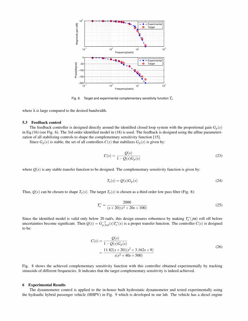
Fig. 8. Target and experimental complementary sensitivity function To

where l is large compared to the desired bandwidth.

5.3 Feedback control

The feedback controller is designed directly around the identified closed loop system with the proportional gain Gp(s)in Eq.(16) (see Fig. 6). The 3rd order identified model in (18) is used. The feedback is designed using the affine parameteri-zation of all stabilizing controls to shape the complementary sensitivity function [15].

Since Gp(s) is stable, the set of all controllers C(s) that stabilizes Gp(s) is given by:

C(s) =Q(s)

1�Q(s)Gp(s)(23)

where Q(s) is any stable transfer function to be designed. The complementary sensitivity function is given by:

To(s) = Q(s)Gp(s) (24)

Thus, Q(s) can be chosen to shape To(s). The target To(s) is chosen as a third order low pass filter (Fig. 8):

T ⇤o =

2000(s+20)(s2 +20s+100)

(25)

Since the identified model is valid only below 20 rad/s, this design ensures robustness by making T ⇤o ( jw) roll off before

uncertainties become significant. Then Q(s) = G�1p,3rd(s)T

⇤o (s) is a proper transfer function. The controller C(s) is designed

to be:

C(s) =Q(s)

1�Q(s)Gp(s)

=11.82(s+20)(s2 +3.162s+9)

s(s2 +40s+500)

(26)

Fig. 8 shows the achieved complementary sensitivity function with this controller obtained experimentally by trackingsinusoids of different frequencies. It indicates that the target complementary sensitivity is indeed achieved.

6 Experimental Results

The dynamometer control is applied to the in-house built hydrostatic dynamometer and tested experimentally usingthe hydraulic hybrid passenger vehicle (HHPV) in Fig. 9 which is developed in our lab. The vehicle has a diesel engine

Polaris Ranger outfitted

Dynamometer

hydraulic hybrid transmission

with custom power−split

Tandem pump/motors

Torque sensor

Flywheel

Charge pump

Hydraulic power supply

Drive shaft

Vehicle

Accumulator

Directional valve

Fig. 9. Top: Hydrostatic dynamometer (rear) connected to an experimental hydraulic hybrid vehicle (front). Bottom: Components of thehydrostatic dynamometer.

and a hydraulic input-coupled power-split transmission, hybridized by a pair of hydraulic accumulators for energy storage.The hydraulic hybrid vehicle is controlled by a 3-level control scheme described in [16, 17] that aims to achieve the driverdemanded vehicle torque in an energy efficient manner. In order to have repeatable testing results, the driver is simulated by avirtual driver controller which is a proportional-integral speed controller. The virtual driver controller, the hybrid powertraincontroller, and the dynamometer controller operate independently of each other (Fig. 10).

The mass of the intended vehicle tested is Mveh = 500 kg and the road/aerodynamic drag in (4) is [18]:

Fdrag =12

CDA f rv2

+Mvehg

fo +3.24 fs

⇣ v44.7

⌘2.5� (27)

where CD = 0.5 is the drag coefficient, A f = 1.784m2 is the frontal area, r = 1.29kg/m3 is the air density, g = 9.31m/s2 isthe acceleration due to gravity, fo = 0.0095 and fs = 0.0035 are the coefficients for rolling resistance. The drag coefficientscorrespond to the vehicle in Fig. 9. The final drive ratio is rd = 3.45 and wheel radius is Rw = 0.3095m. Note that the targetvehicle parameters do not need to correspond to a vehicle that has been built.

The Environmental Protection Agency’s (EPA) Urban Dynamometer Driving Schedule (UDDS) and Highway FuelEconomy Driving Schedule (HWFET) with some modifications1 are used as reference speed profiles to test the efficacy ofthe dynamometer control scheme. For verifying the performance of the dynamometer control, the HHPV is operated incontinuously variable transmission (CVT) mode in which the accumulator pressure is kept at a nearly constant pressure.

Figures 11-12 show the actual vehicle-dyno shaft speed w and the virtual vehicle speed wveh for the modified UDDSand HWFET drive cycles respectively. The errors in tracking the virtual vehicle speed are shown in Fig. 13. Despite theerrors being larger during high acceleration/decceleration, the actual speed tracks the virtual vehicle speed reasonably withRMS errors of 17 rpm (UDDS) and 11 rpm (HWFET) which are 1.25% and 0.8% of the mean speeds of the cycles. Thisdemonstrates the effectiveness of the dyno-speed controller design in section 5.

1The drive cycle are modified so that speed does not violate the low speed limit of the dynamometer hardware configuration.

Fig. 10. Dynamometer testing of hydraulic hybrid vehicle involves three independent controllers: dynamometer controller, hydraulic hybridpowertrain controller and virtual driver controller.

400 600 800 1000 1200 1400 1600

400

600

800

1000

1200

1400

1600

1800

time

Ou

tpu

t S

pe

ed

(rp

m)

Virtual Vehicle SpeedActual Shaft Speed

Fig. 11. Actual speed and virtual vehicle speed of the vehicle-dyno shaft while driving the modified UDDS.

200 300 400 500 600 700 800 900 1000

400

600

800

1000

1200

1400

1600

1800

time

Ou

tpu

t S

pe

ed

(rp

m)

Virtual Vehicle Speed

Actual Shaft Speed

Fig. 12. Actual speed and virtual vehicle speed of the vehicle-dyno shaft while driving the modified HWFET.

200 400 600 800 1000 1200 1400 1600−100

−50

0

50

100

Time [sec]

Sp

ee

d T

rack

ing

Err

or

[rp

m]

Speed Tracking Error

RMS = 16.6 rpm

200 300 400 500 600 700 800 900 1000−80

−60

−40

−20

0

20

40

60

Time [sec]

Sp

ee

d T

rack

ing

Err

or

[rp

m]

Speed Tracking Error

RMS = 11.2 rpm

Fig. 13. Error between actual speed and the desired virtual vehicle vehicle-dyno shaft speed while driving the UDDS (top) and HWFET(bottom) cycles.

582 584 586 588 590 592 594 596 598 600−20

−10

0

10

20

30

Time [s]

Torq

ue

Real−time Tveh

Post−processed Tveh

Fig. 14. Vehicle torque obtained using real-time observer Eq.(20) and using off-line calculation in portion of the modified UDDS test.

Time[sec]

200 400 600 800 1000 1200 1400 1600

Torq

ue[N

m]

-50

-40

-30

-20

-10

0

10

20

30

40

Applied torque

Des. torque-output spd

Des torque-vir. veh

Time[sec]

550 600 650 700 750 800

Torq

ue[N

m]

-50

-40

-30

-20

-10

0

10

20

30

Applied torque

Des. torque-output spd

Des torque-vir. veh

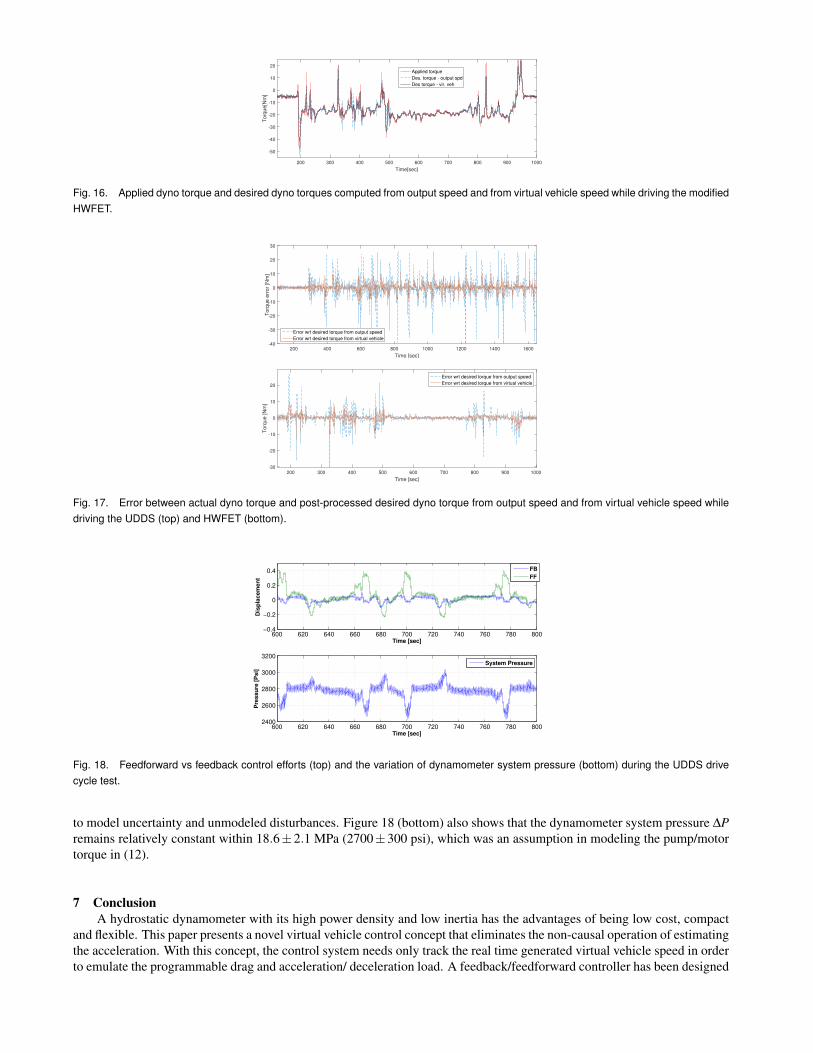
Fig. 15. Applied dyno torque and desired dyno torques computed from output speed and from virtual vehicle speed while driving the modifiedUDDS. Top: full cycle; Bottom: zoomed in view.

The real-time vehicle torque estimate Tveh obtained using the observer (20) is verified by comparing it with Tveh computedoff-line from (19) using the measured shaft speed w(t) and the torque cell measurement Tmeas(t), where w(t) is obtained inconjunction with a 2.5Hz 2nd order zero-phase low pass filter. A portion of this comparison is shown in Fig. 14 which showsthat they are virtually identical.

In order to verify that the dynamometer is applying the correct load, the actual dyno torque and the desired dyno torqueare calculated in post-processing and compared. The actual dyno torque TDyno is estimated based on the torque measurementTmeas and the dynamics of JDyno :

TDyno = JDynow�Tmeas

The desired dyno torque is computed based on Eq. (6). There are two options for the speed profile wveh in (6): i) the actualmeasured speed w, or ii) the virtual vehicle speed wveh. Since the entire profile is known, either profile can be differentiatedoff-line, in conjunction with a zero-phase low pass filter (5th order Butterworth filter with 5 rad/s cutoff) to obtain theacceleration. Figures 15-16 show the torque tracking performance for the UDDS and HWFET respectively with respect tothe desired torque profiles. Figure 17 shows the torque tracking errors. When the desired torque is computed using the outputspeed w, the RMS torque errors are 6.1 Nm (UDDS) and 3.9 Nm (HWFET). However, when they are computed using thevirtual vehicle speed wveh, the RMS torque errors are only 2.6 Nm (UDDS) and 1.6 Nm (HWFET). From Fig. 15-bottom,it is seen that the larger error when w is used to compute the desired torque can be attributed to the oscillatory nature of wrather than TDyno itself. This highlights the inherent difficulty in estimating w even in post-processing (and more so in realtime for feedback) and the advantage of the virtual vehicle control concept.

Figure 18 (top) shows the feedforward and feedback control efforts in terms of the pump/motor displacements. Asintended from the controller design, the feedforward component is more dominant in providing the necessary actuation totrack the desired virtual vehicle speed. However, the feedback component is also necessary to eliminate tracking error due

Time[sec]

200 300 400 500 600 700 800 900 1000

To

rqu

e[N

m]

-50

-40

-30

-20

-10

0

10

20Applied torque

Des. torque - output spd

Des torque - vir. veh

Fig. 16. Applied dyno torque and desired dyno torques computed from output speed and from virtual vehicle speed while driving the modifiedHWFET.

Time [sec]

200 400 600 800 1000 1200 1400 1600

To

rqu

e e

rro

r [N

m]

-40

-30

-20

-10

0

10

20

30

Error wrt desired torque from output speed

Error wrt desired torque from virtual vehicle

Time [sec]

200 300 400 500 600 700 800 900 1000

To

rqu

e [

Nm

]

-30

-20

-10

0

10

20

Error wrt desired torque from output speed

Error wrt desired torque from virtual vehicle

Fig. 17. Error between actual dyno torque and post-processed desired dyno torque from output speed and from virtual vehicle speed whiledriving the UDDS (top) and HWFET (bottom).

600 620 640 660 680 700 720 740 760 780 800−0.4

−0.2

0

0.2

0.4

Time [sec]

Dis

pla

cem

en

t

600 620 640 660 680 700 720 740 760 780 8002400

2600

2800

3000

3200

Time [sec]

Pre

ssu

re [

Psi]

FB

FF

System Pressure

Fig. 18. Feedforward vs feedback control efforts (top) and the variation of dynamometer system pressure (bottom) during the UDDS drivecycle test.

to model uncertainty and unmodeled disturbances. Figure 18 (bottom) also shows that the dynamometer system pressure DPremains relatively constant within 18.6±2.1 MPa (2700±300 psi), which was an assumption in modeling the pump/motortorque in (12).

7 Conclusion

A hydrostatic dynamometer with its high power density and low inertia has the advantages of being low cost, compactand flexible. This paper presents a novel virtual vehicle control concept that eliminates the non-causal operation of estimatingthe acceleration. With this concept, the control system needs only track the real time generated virtual vehicle speed in orderto emulate the programmable drag and acceleration/ deceleration load. A feedback/feedforward controller has been designed

for this purpose. The control concept has been experimentally validated. The dynamometer is now being actively utilized inthe laboratory for testing and evaluating different hydraulic hybrid vehicle designs and control schemes.

The control performance is acceptable for assessing vehicle fuel economy by controlling the pump/motor displace-ment alone. System identification results indicate that the bandwidth of the pump/motor is indeed somewhat limited (2.5rad/s). Future work will consider using the proportional directional control valve in Fig. 2 as an active control elements forimproving the control.

Acknowledgements

This material is based upon work performed within the Center for Compact and Efficient Fluid Power (CCEFP) whichis supported by the National Science Foundation under grant number EEC-0540834.

References

[1] S. Raman, N. Sivashankar, W. Milam, W. Stuart, and S. Nabi, “Design and Implementation of HIL Simulators forPowertrain Control System Software Development,” Proceedings of the American Control Conference, San Diego, CA,1999

[2] H. J. Kohring, “Design and Construction of a Hydrostatic Dynamometer for Testing a Hydraulic Hybrid Vehicle,” M.S.-A Thesis, Department of Mechanical Engineering, University of Minnesota, Twin Cities, 2012.

[3] J.-S. Chen, “Speed and Acceleration Filters/Estimators for Powertrain and Vehicle Controls,” SAE Technical paper,2007-1-1599, April 2007

[4] J. Longstreth, F. Sanders, S. Seaney, J. Moskwa et. al. “Design and Construction of a High-Bandwidth HydrostaticDynamometer”, SAE Technical Paper 930259, 1993, DOI: 10.4271/930259.

[5] J. Lahti and J. Moskwa, “A Transient Test System for Single Cylinder Research Engines with Real Time Simula-tion of Multi-Cylinder Crankshaft and Intake Manifold Dynamics,” SAE Technical Paper, 2004-01-305, 2004, DOI:10.4271/2004-01-0305.

[6] A. S. Heisler, J. Moskwa and F. Fronczak, “The Design of Low-Inertia, High-Speed External Gear Pump/motors forHydrostatic Dynamometer Systems,” SAE Technical Paper 2009-01-1117, 2009.

[7] M. Holland, K. Harmeyer and J. Lumkes Jr., “Design of a High-Bandwidth, Low-cost Hydrostatic Dynamometer withElectronic Load Control,” SAE Technical Paper: 2009-01-2846.

[8] F. Tavaresm, R. Johri, and A. Salvi, “Hydraulic Hybrid Powertrain-in-the-loop integration for analyzing real-world fueleconomy and emissions improvements,” SAE Technical Paper 2011-01-2275, 2011. DOI:10.4271/2011-01-2275.

[9] Y. Wang, Z. Sun, and K. A. Stelson, “Modeling, Control, and Experimental Validation of a Transient Hydrostatic Dy-namometer,” IEEE Transactions on Control Systems Technology, volume 19, number 6, Nov. 2011

[10] G. R. Babbitt, R. L. Bonomo and J. J. Moskwa, “Design of an integrated control and data acquisition system for ahigh-bandwidth, hydro- static, transient engine dynamometer,” Proceedings of the 1997 American Control Conference,pp. 11571161, Albuquerque, New Mexico, 1997.

[11] G. R. Babbitt and J. J. Moskwa, “Implementation details and test results for a transient engine dynamometer andhardware in the loop vehicle model,” Proceeding of the 1999 IEEE International Symposium on Computer Aided ControlSystem Design, Hawaii, pp. 569574, 1999.

[12] I. Stringer and K. Bullock, ”A Regenerative Road Load Simulator,” SAE Technical Paper 845115, 1984,doi:10.4271/845115.

[13] R. Zhang and A. G. Alleyne, “Dynamic Emulation Using an Indirect Control Input,” ASME Journal of Dynamic Sys-tems, Measurement, and Control, 127:1, pp.114-124, 2005

[14] J.D. Van de Ven, M.W. Olson and P.Y. Li, “Development of a hydro-mechanical hydraulic hybrid drive train withindependent wheel torque control for an urban passenger vehicle,” in Proceedings of the 2008 International Fluid PowerExposition (IFPE), Las Vegas, NV, 2008.

[15] G. C. Goodwin, S. F. Graebe and M. E. Salgado Control System Design. Prentice Hall, 2000.[16] P. Y. Li and F. Mensing, “Optimization and Control of a Hydro-Mechanical Transmission Based Hydraulic Hybrid

Passenger Vehicle,” 7th International Fluid Power Conference (IFK), Aachen, Germany, March, 2010.[17] K. L. Cheong, Z. Du, P. Y. Li and T. R. Chase, “Hierarchical Control Strategy for a Hybrid Hydro-mechanical trans-

mission (HMT) power-train,” Proceedings of the 2014 American Control Conference, Portland, OR, June 2014.[18] T. D. Gillespie, Fundamentals of Vehicle Dynamics, Society of Automotive Engineers, Inc., Warrendale, PA, 1992.