Purdue UniversityPurdue e-Pubs

Open Access Theses Theses and Dissertations

Spring 2015

Drop volume modulation via modulated contactangle in inkject systemsAaron FultonPurdue University

Follow this and additional works at: https://docs.lib.purdue.edu/open_access_theses

Part of the Mechanical Engineering Commons

This document has been made available through Purdue e-Pubs, a service of the Purdue University Libraries. Please contact epubs@purdue.edu foradditional information.

Recommended CitationFulton, Aaron, "Drop volume modulation via modulated contact angle in inkject systems" (2015). Open Access Theses. 522.https://docs.lib.purdue.edu/open_access_theses/522

Graduate School Form 30 Updated 1/15/2015

PURDUE UNIVERSITY GRADUATE SCHOOL

Thesis/Dissertation Acceptance

This is to certify that the thesis/dissertation prepared

By

Entitled

For the degree of

Is approved by the final examining committee:

To the best of my knowledge and as understood by the student in the Thesis/Dissertation Agreement, Publication Delay, and Certification Disclaimer (Graduate School Form 32), this thesis/dissertation adheres to the provisions of Purdue University’s “Policy of Integrity in Research” and the use of copyright material.

Approved by Major Professor(s):

Approved by:

Head of the Departmental Graduate Program Date

Aaron Fulton

Drop Volume Modulation via Modulated Contact Angle in Inkject Systems

Master of Science in Mechanical Engineering

George ChiuChair

Peter Meckl

Jeffrey Rhoads

Oman Basaran

George Chiu

Ganesh Subbarayan 4/30/2015

DROP VOLUME MODULATION VIA MODULATED CONTACT ANGLE IN

INKJECT SYSTEMS

A Thesis

Submitted to the Faculty

of

Purdue University

by

Aaron Fulton

In Partial Fulfillment of the

Requirements for the Degree

of

Master of Science in Mechanical Engineering

May 2015

Purdue University

West Lafayette, Indiana

ii

TABLE OF CONTENTS

Page

LIST OF v

.

LIST OF VARIABLES. vii

i

1. IN ..1

2. BACKGROUND ......4

2.1 Natural Jetting Phenomena. ....4

2.2 Meniscus ....8

2.3 ...12

2.4 .15

3. ..........17

3 17

3 17

3.3 Analytical Model ...19

3.3 ...20

3.3.2 Jet Breakup and . 23

3.3 26

3.4 Fluid Properties 30

3.5 Model Assumptions, Selections, and Justifications .31

iii

Page

4 .35

4 35

4 .36

4 36

5. RES 40

5.1 Experimental Methods 40

.44

5.3 Frequency Stability . 48

5.4 Parameter Sweep Based Studies 48

5.5 Jettability Regions 49

64

LIST OF REFEREN ................ .65

APPENDICES

Appendix A. Fluid 69

0

iv

LIST OF TABLES

Table Page

1. Experimental fluid properties of SU-8 2002 and Palladium hexadecane thiolate in toluene............................................................................................................................30

2. Computational fluid properties of SU-8 2002 and Palladium hexadecane thiolate in toluene 69

v

LIST OF FIGURES

Figure Page

1. Comparison of prior works to work presented, inkjet geo .6

2. Nozzle meniscus features and dimensions . ....11

3. The evolution of meniscus shapes ..12

4. Nozzle meniscus features and dimensions .....23

5. Oscillatory phases of a moving droplet in free space 26

6. Experimental Setup and generic nozzle profile of TIPS nozzle Experimental results compared to prior 36

7. CFD geometry, nozzle, meshing, and waveform ...38

8. Experimental results compared and contrasted with work by Basaran and analytical and

computational methods .....42

9. Experimental results compared 44

10. Simulation of effects of manipulated c 6

51

ty . 2

13. Castrejón- overlaid .. 3

14. Application of a 90 degree con .. 4

15. Application of a 70 degree con .. 5

16. Application of a 35 degree con . 6

17. Application of a 7 d ......57

18. Stability diagram of a 40 de 58

vi

Figure . Page

19. Stability mapping of 0 Pa back pressure 61

20. Stability mapping of 30 Pa back pressure ....60

21. Stability mapping of 60 Pa back pressure ... 61

22. Stability mapping of 90 Pa back pressure .. 62

23. Contact angle 90 and experimental data, and data fro .....70

24. Contact angle 61.66 and experimental data, and data fro ....71

25. Contact angle 33.33 and experimental data, and data . 72

26. Contact angle 5 and experimental data, and data from [8], [10], and .....73

vii

LIST OF VARIABLES

Froude number

c Concentration of species

Time delay between deposited drops

d Distance between firings

Print-head scanning speed used for determining drop flight speed

Bo Bond number

g Acceleration of gravity

Density of working liquid

Density of gas (usually air, with the notable exception of boiling)

D Diameter

Ambient pressure

Pressure relative to ambient pressure

Dimensionless pressure

Radius of nozzle

We Weber number

Re Reynolds number

Oh Ohnesorge number

Ca Capillary number

Surface tension

viii

Capillary time

Viscosity

Electric potential

Volume fraction

Phase variable

Fluid velocity

Interface thickness

Species mobility

Force of surface tension

Mixing energy density

G chemical potential

p Pressure

Pressure of saturated vapor

Ambient pressure

Latent heat of vaporization

T Temperature

Saturated temperature

Temperature of vapor

Boltzmann constant

R Universal gas constant

Enthalpy of vaporization

Molecular weight

Thermal conductivity of vapor

Thermal conductivity of liquid

Mass flux

H Mean curvature

ix

Radius of curvature

Radius of tubes

Receding contact angle

Advancing contact angle

Contact angle

Back pressure

Capillary pressure

d Diameter of tapered nozzle

Taper angle

z Axial coordinate

r Radial coordinate

l Distance away from the free surface from the pressure impulse

Pressure waveform, Clausius-Clapeyron for thermal inkjet

Time change during pressure impulse

t Time

Jet velocity upon leaving the ballistic region

The duration time of flow focusing through the curved surface

Effective distance, or height

The distance between the meniscus and the horizontal plane

n Number of mols

A fluid particle being ejected from the axial acceleration region into the ballistic region at this time

Rayleigh instability wavelength

Radius of jet

Approximate capillary time

Radius droplet

x

Viscous dissipation function

t* Non-dimensional time

Deformation directions of droplet

y Mass coordinate of droplet

z Mass coordinate of droplet

Solution viscosity

Particulate contribution to viscosity

Solute viscosity

Diffusion coefficient

xi

ABSTRACT

Fulton, Aaron. M.S.M.E, Purdue University, May 2015. Drop Volume Modulation via Modulated Contact Angle in Inkjet Systems. Major Professor: George T.-C. Chiu, School of Mechanical Engineering.

To date, there are limited options in the ability to adjust feature sizes when inkjet

printing. The reduction of nozzle size has been the primary method by which smaller features are

created. Prior attempts to reduce feature sizes have all come with some restriction or another, as

they are only accessible on certain systems, are difficult to manufacture, tune, cause clogging, etc.

Few attempts to create droplets of smaller radii than that of the nozzle from which they are

produced have been successful. Additionally, many fluids cannot be jetted whatsoever. Existing

methods pertain largely to piezoelectric inkjet printing and time scale manipulation of negative

pressure pulse versus fluid properties, rendering them inapplicable to thermal inkjet technologies

as these are unable to apply a negative pressure pulse. In this work, a simple method for drop

volume control in inkjet systems is proposed in which the stable drop volume can be reduced by

an order of magnitude with a constant nozzle radius by adjusting the back pressure (pressure

applied in the opposite direction of the ejection in a nozzle) in the reservoir that supplies the print

head. However, this technique carries with it a surprising benefit, the increase in printability in

regions previously unavailable. To evaluate this effect across many printing platforms,

simulations of the effects of back pressure were performed. Computational fluid dynamics in its

many forms (phase field, level set, etc.) has been historically found to be extremely accurate for

predicting inkjet phenomena [1-16]. Using only the two most prominent forms of inkjet, thermal

xii

and piezo, to represent all inkjet phenomena is justified as most inkjets simply are the application

of a brief pressure pulse at the back of a nozzle. These two inkjet varieties are no different, the

only difference is its point of origin. In these, the back pressure is regulated and the fluid

meniscus is allowed to come to rest and then a positive pressure impulse is applied creating a

droplet. From this, droplet sizes, stability, and velocities are recorded. These results are then

corroborated by rigorous analytical modeling. The results of this modelling can be used to

generate mappings of printability in regards to contact angle; this allows for the design of both

dynamic printing waveforms and static application techniques. The general contribution of this

work, is not in the novelty of its results or the methods by which they are understood, as they

have all been developed in some fashion previously, but rather the new combinations and

resulting conclusions. Prior works in this area have all explored some facet of the implicit

manipulation of meniscus shapes prior to fluid ejection, but by viewing this phenomenon from a

more explicit viewpoint the result is more broadly applicable and understandable.

1

CHAPTER 1. INTRODUCTION

At its simplest level, inkjet printing is simply the deposition of a pattern. The inkjet

printing of a fluid is the deposition of the fluid to create the pattern. It has long been understood

that the diameter of the pattern s smallest feature is created by the spread droplet driven out of a

printhead nozzle. Previous works have largely determined that the size of the droplet preceding

the impact cannot be smaller than the nozzle diameter. This presents a difficulty in printing as for

different feature sizes you must either use a small nozzle and print several droplets or swap

between large and small nozzles throughout the printing process. Additionally, small nozzles clog

and present many further complications. This issue gains importance from the fact that in inkjet

printing it is often desirable to print ever smaller features while still being able to quickly fill

large area patterns as well. As a result, it is useful to be able to attain both small droplet sizes and

large droplet sizes from the same nozzle, while dynamically changing some parameter. Basaran

et al. [1] demonstrated that by careful control of the driving waveform of a piezo-inkjet

(changing the shape of the air-fluid interface, the meniscus) and then pushing the fluid back down

then pulling the fluid once again, he could achieve far smaller droplets. The explanation given

indicated that this needed to be done dynamically and that the event is too complex to break down

much further than the timings of the impulses. Similar approaches were seen [1, 7]. These all

suggested that there needs to be more investigation into drop volume modulation for inkjet

nozzles. Additionally, these methods of creating small droplets from large nozzles were exclusive

to piezoelectric inkjets with no apparent counterpart for thermal inkjets. By coupling all of the

research pieces found in tandem with a greater understanding of the underlying phenomena, this

2

dynamic phenomena can be broken down into a static initial condition and a dynamic pulse

phase. This allows for these previous research efforts to be interpreted and applied to all types of

inkjets as opposed to strictly piezoelectric.

This work proposed a unifying approach to analyze droplet stability reported in prior

works [1, 7, 13]. Specifically, we will attempt to identify the commonality between the reduction

of droplet volume and the preconditioning applied by each respective research group [1, 7, 13].

By changing the time at which the initial conditions are applied, a relatively complex phenomena

is simplified. This allows for prior analysis techniques to be applied with modifications.

Accordingly, this allows the application of this approach to easily modify current printing

techniques by simply changing their initial conditions before each discrete jetting event. To

examine the phenomena from this perspective, natural corollaries are examined, numerical results

are generated, and analytical solutions are generated from the modifications of previous works.

This is then combined to give a complete perspective of the phenomena from multiple

complementary viewpoints.

Much like traditional fluid printing techniques, functional printing uses the same methods

to deposit functional materials. In functional inkjet printing applications, it may be desirable to

enable the tuning of the drop volume and speed. Accordingly, one can control the feature size

created by the impact of a droplet on a substrate, dot gain, to accommodate multiple size scales

within a device at a high throughput. This becomes an issue when printing large space filling

areas and small features within the same device, such as in a comb capacitor. The capacitive

elements require thin lines where a small drop volume is necessary, while the contact pads require

a larger area, where a large drop volume would optimize throughput. To date, there are limited

options in the ability to modulate drop volume with a single nozzle. Existing methods pertain to

piezoelectric inkjet printing, which control the waveform and time scale manipulation of the

3

capillary, viscous, and inertial flow behaviors, rendering them inapplicable to thermal inkjet

technologies [8-9]. Specifically, the waveform manipulation used to create smaller droplets is a

departure from the traditional square waveform, and cannot be replicated by thermal inkjets. It is

this difference that currently limits inkjet drop volume modulation. A method for drop volume

control in thermal inkjet systems is proposed in which stable drop volume can be reduced by an

order of magnitude with a constant nozzle radius. It is shown that adjusting the back pressure in

the reservoir that supplies the print head is a feasible method to form droplets with radii smaller

than that of the nozzle. Additionally, in functional inkjet printing many fluids have less than ideal

properties for stable droplet creation. To increase the printability of any given fluid is a desirable

attribute. By manipulating the nature of the velocity and profile of a fluid jet, one can also

increase the printability of many fluids that are otherwise unsuitable for inkjet printing.

To determine the extent and nature of the effect of high back pressure on the process of

jetting fluid from an inkjet, the back pressure is regulated through the use of a syringe, and

measured throughout the printing process and droplet masses and velocities are found for each

deposition. To form a complete model of this phenomena, the data for these tests are collected

through a range of heights, pressures, and fluids, and evaluated for droplet quality and satellite

formation. These results are justified through theoretical and numerical analysis [7-9, 16], leading

to a view that droplets of a smaller diameter than that of a nozzle is driven by meniscus shaping,

driving waveform, inkjet geometry, and fluid properties. Additionally, the results are subjected to

traditional non-dimensional analysis for prediction of droplet stability and droplet sizing through

numerical methods parameter sweep and compared to similar results [7-9]. Computational

mappings of droplet stability regions are found to corroborate the experimental and theoretical

findings.

4

CHAPTER 2. BACKGROUND

2.1 Natural Jetting Phenomena

Worthington jets are a common occurrence: a rock falls in a pool and out comes a thin

splash, this can be seen in Figure 1. A. This resulting splash emanates from a thin jet, a

Worthington jet [18]. A Worthington jet consists of three components core to its behavior, all

stemming from the collapse of a cavity in a body of fluid as created by an object impacting that

fluid [18]. The size and shape of a cavity correlates to the force of impact and the size and shape

of the impacting object. These factors are encapsulated by the Froude number. This is

demonstrated in Figure 1. A. The size of the Froude number directly correlates with the size of a

cavity created in any fluid impacted by any object and accordingly the magnitude of the force

with which it collapses as seen below,

. (1)

A cavity in a fluid collapses because of a discontinuity in pressure due to a dissimilarity in

surface tension. This causes the fluid walls to impact each other generating a vertical jet. Jet

break up is caused by the capillary deceleration due to capillary forces found in every fluid entity,

and this perturbs the liquid at the tip which produces a sinusoidal jet shape. This sinusoidal shape,

can be caused by capillary deceleration or any other deceleration additionally present. The first

part of a Worthington jet is the axial acceleration region which occurs during the collapse of the

jet, in which the radial momentum of the incoming liquid, due to the collapse of a cavity, is

5

converted to axial momentum. The fluid particles then leave the axial acceleration region and

enter the ballistic region. In this region, fluid particles experience no further acceleration and

move constantly with the velocity obtained at the end of the axial acceleration region. In this

region, the velocity can be assumed to be axial. In the jet tip region, the jet breaks into a droplet.

This droplet diameter is far smaller than the characteristic length of the impacting object and

accordingly the void created by it. This presents an opportunity to apply a similar approach to

inkjets, yielding a similar reduction in drop volume.

Jetting from a nozzle with an applied back pressure and an accommodating receding

contact angle is similar to the Worthington jet phenomena. The meniscus caused by the applied

back pressure simulates the cavitation associated with the impact of an object on a fluid body.

Normally, the discontinuity in pressure is caused by fluid trying to refill the cavity created by the

impact, the fluid collapses and this causes a jet. In an inkjet, the discontinuity in pressure is no

longer just a product of the difference in surface tension trying to refill a cavity. Instead, the

deceleration which causes the corollary to the natural push-pull, is a product of capillary

deceleration and oscillations of the fluid surface. In an inkjet, an additional push-pull force is

applied to create a droplet, recreating the forces that affect the natural jet by creating the same

sequence of positive and negative pressures in roughly the same time scales, with the only

difference being their amplitudes.

6

Figure 1. Comparison of prior works [3, 8] to work presented, inkjet geometries and input waveforms, all images shown are that of independently created work.

In nature, the phenomena can be seen with the impact of a droplet on a fluid reservoir. As

seen in Figure 1.A, a 0.74 cm droplet is seen falling into a glass of water, which causes a cavity to

form. Upon collapse of the cavity caused by the droplet, the fluid transitions through an axial

7

acceleration region (I) in Figure 1.A where the horizontal components are converted to vertical

acceleration causing velocity to grow in this direction, and the collapsing sides impede side

upward expansion allowing for the fluid to be channeled through the center. Additionally, the

pressure wave is focused behind the center of the jet, further driving flow in this region. It is at

this point it enters the ballistic region (II) where it is no longer accelerated but rather decelerated

via capillary action, causing perturbation, which causes a wavy profile along the fluid wall, which

grows due to dissimilar surface tension (Marangoni flows) leading to the jet tip region (III) where

the stream eventually breaks into any number of droplets as depending upon forcing function

(impacting object, characterized by the Froude number) and the fluid. In Figure 1.B, [3], a 35

micron nozzle was reproduced in simulation representing the first attempt to manipulate drop

volume via a dynamic pressure pulse waveform. This was characterized by a negative impulse

followed by a positive impulse, then another negative impulse. After this, to aid in refill, a final

positive impulse is applied. The nozzle was attached to an actuated capillary tube causing a

pressure pulse in proportion to voltage. The working fluid was a 50% by weight glycerol and

water mixture. The rising and falling edges of the voltage correspond to the spikes of pressure

seen in the tube. The waveform applied consisted of a succession of three square wave voltage

pulses with a negligible transition rise profile, the first negative, the second positive, and the third

negative. These pulses have peak amplitudes of V= -46 V, 56 V, and -46 V and last for t=36 s,

18 s, and 36 s respectively. The radius as found by experiment was 16 m and was predicted

by a simulation created in this work to be 16.73 m. This is a reduction from the droplet volume

produced by a single square wave impulse of 100 V which yields 45 m droplets. The

dimensionless pressure pulse magnitude is found in respect to voltage by . This is in

turn related to the capillary time, This is then measured against the ambient

relative pressure, . = = / . In Figure 1.C, [8] a notched nozzle design is presented in

8

which 80% by weight glass microspheres and water solution, was fired from the nozzle. The

method presented utilized a pull-push-pull method waveform. This waveform caused a collapse

axially aligned with the outlet driving an extremely small droplet to be created from a large

nozzle. This created a reduction in clogging and a considerable increase in the type of fluids

printable. The droplet size, as produced from a large scale 2 mm nozzle was roughly 110 m. It

should be noted that back-pressure-based meniscus manipulations fail to achieve such reductions

on the large scale (mm) but fared far more favorably on small scale ( m) that yielded a reduction

of droplet size from 100 m to 38 m. Back-pressure-based results are nearly identical to the

above. This leads to the assumption that smaller length and time scales suppress the Worthington

jet phenomena as collapse becomes less and less pronounced, and instead a similar phenomenon

begins to take its place as focusing becomes more prominent. Focusing is where the flow is

channeled toward the center of a nozzle by both the no-slip condition and additional mass held in

the meniscus and the curvature of the focusing of pressure on the center of the free surface

generating high pressure regions causing faster flow in the center of the nozzle. Collapse

dominates when the meniscus and/or nozzle are large. Focusing dominates when the nozzle or

meniscus is small. Both are always at play with any jetting with an initially curved free fluid

surface, however, the effects of focusing are always fully maintained while collapse singularity

dynamics are drastically reduced with increasingly lower menisci. In Figure 1.D, the effects of

back pressure are demonstrated on the same nozzle as designed by Castrejón-Pita in 2011 [6]. In

this example, the meniscus achieves a contact angle of 5 degrees prior to jetting, this

demonstrates the effect highlighted in this work [7]. The working fluid is acetone.

2.2 Meniscus

Throughout this entire work, a general nomenclature and geometric set of identities will

be used. In the case of generic laws, they may be presented in their traditional Cartesian (x,y,z)

9

set of coordinates and these are arbitrarily set. However, for all derivations presented in respect to

s nozzle. The point of

origin is set at the axis symmetric base of the inkjet nozzle from which the pressure pulse used to

drive the fluid flow appears. The coordinate direction r is that of the radial direction of the nozzle

as seen in Figure 2. In the

description of inkjet printing and the effects of backpressure the explicit parameter, backpressure

is obviously the most convenient parameter by which to examine relationships between its

modulation and the jetting observed. However, this yields an unclear relationship. Instead of back

pressure, a more appropriate parameter to observe is that of the meniscus, which is controlled by

the fluid properties and the back pressure. The meniscus shape is completely described in a small

tube by the contact angle. This makes the contact angle, fluid properties, and the back pressure

inextricably linked. Accordingly, the explicit parameter backpressure is applied but it is the

individual fluids reaction to that back pressure in the form of contact angle that best indicates the

underlying physics of the drop volume reduction phenomena. Governing the meniscus is the

Young Laplace equation, which is a nonlinear partial differential equation representative of the

change in capillary pressure over an interface between two dissimilar fluids in static contact. This

pressure change is due to surface tension,

, (2)

. (3)

the mean curvature, H, the average of the principal curvatures, , is the pressure change across

the infinitesimally thin interface,

. (4)

10

in a narrow tube of circular cross-section, this reduces to,

(5)

where is

, (6)

accordingly,

(7)

From that one can obtain the expression for the radius of curvature with respect to back pressure.

Assuming the contact angle does not exceed the receding contact angle for a given fluid-gas-

substrate triple point, this allows for the radius of curvature as represented by a circle to vary

smoothly from the radius of and infinite diameter circle and accordingly flat interface to that of a

perfect hemisphere of radius at which point all fluids begin to slip, and recede into the ink

reservoir. Accordingly back pressure relates to contact angle,

. (8)

However, not all nozzles are perfect cylinders but rather they consist of angled axis symmetric

walls, as a result, the equation must be adapted accordingly with a change in constant and the

. (9)

11

Figure 2. Nozzle meniscus features and dimensions.

Accordingly, as many fluids were tested in the course of research, acetone and e-gain

(Galistan) as examples, the parameter varied was contact angle. This was due to the fact that

certain fluids did recede very early on with respect to back pressure. Whereas, those with a larger

surface tension did recede later. Accordingly, all maps will be presented in terms of achieved

contact angle, if contact angle is less than that of the receding contact angle for a given fluid-gas-

substrate combination. All focusing phenomena is due to contact angle and is largely unaffected

by the change in pressure across the interface as the driving forces seen in an inkjet are several

orders of magnitude larger than any seen at the fluid-gas interface. An example of this is the

receding pressure of acetone, assuming a receding contact angle of 5 degrees, is 25 Pa for this

respective fluid as for all fluids the contact angle achieve for a given back pressure is different see

eq. 23-27. Whereas, for e-gain it is closer to 710 Pa. Before receding, they both obtain the exact

same meniscus shape. This is the key factor in jetting and will be mapped later as it affects jetting

phenomena. A contact angle of 90 degrees results in a perfectly flat fluid-gas interface, and that

of 0 degrees is a perfect hemispherical silhouette of the same radius of the tube, so with no

gravity or other body forces at zero pressure the surface is flat, and at 24.81 Pa the meniscus has a

radius of curvature of 67.5 m.

12

Figure 3. The evolution of meniscus shapes in a 67 micrometer nozzle with an estimated zero degree taper as back pressures are applied assuming Toluene as reported in Appendix: A, (A) back pressure of 0, (B) back pressure of 8.33 Pa, (C) back pressure of 16.66 Pa (D) back

pressure of 24.8 Pa.

When comparing the methods by which droplet volume is reduced by explicit or implicit

meniscus pre-conditioning, it must be emphasized that with Basaran [1], and the simulations

presented in this work, the primary mechanism seen is flow focusing through a curved meniscus

[7]. Whereas, with Castrejón-Pita [6] the primary mechanism of jetting is collapse based, and the

conversion of horizontal momentum to axial momentum. However, this is only for the large-scale

system as the small-scale system seems to have a greatly reduced efficacy in creating small

droplets as the change in drop volume changes from two orders of magnitude to one which is the

same as the work as produced by Basaran and in this study [1]. This is likely due to viscous terms

becoming more dominant on a smaller scale, allowing for flow focusing to function as before, but

greatly reducing the effects of collapse dynamics.

2.3 Piezoelectric Inkjets

To fully understand the phenomena seen in the thermal inkjet system, we examined the

same phenomena in a well-defined piezoelectric inkjet system and characteristically similar

13

thermal inkjet system. The reason for this choice is twofold, thermal inkjet details of our

simulated nozzle are intellectual property of Hewlett Packard, and they are computationally

intensive as they take weeks as opposed to hours. Comparable results were obtained when using

level set and phase field numerical methods when sufficiently tight meshing was applied; the

results for phase field are presented. When using a fixed mesh approach for modelling fluids, a

number of approximations must be made, forcing the defining of boundary conditions above as

volumetric sources or sinks. In the phase field method, the interface dynamics of the two-phase

flow is governed by a Cahn-Hilliard equation [17], which tracks the diffuse interface separating

the two distinct phases via spinodal decomposition (see Section 3.5). We ignore phase changes

across the interface as the droplets are large enough that, through the analysis outlined by Boley

in 2009 [3], we can determine that the evaporation is less than 1% of the total volume within the

flight time shown. Accordingly, for the shown simulation the volume fraction is defined to be

, (10)

where is the dimensionless phase variable; varying between -1 and 1, where -1 and 1 are

assigned to be one of the two pure fluids respectively . The density, , and the

viscosity, , of the fluid are smoothly varied across the interface via,

, (11)

. (12)

Relating the surface tension to interface thickness yields,

(13)

( ) -Hilliard [17]

equation tracks the diffuse interface separating immiscible phases. The diffuse interface is

14

This

describes the process of phase separation, by which the two components of an immiscible binary

fluid spontaneously separate. The Cahn-Hilliard equation is a fourth-order partial differential

equation, so posing it in its respective weak form results in the presence of second-order spatial

derivatives, and the problem could not be solved using a Lagrangian element formulation. A

popular method to solve this is to rephrase the problem as two coupled second-order equations. In

COMSOL, the Cahn-Hilliard equation is dealt with by the implementation of these two

coefficient form PDEs in time discrete form,

, (14)

(15)

where is the species mobility , , is the fluid velocity , is the mixing

energy density

interface thicknesses was determined to be sufficient at the traditional initial guess for the

following simulations as it is found to govern the equilibrium solution,

. (16)

The liquid velocity field in the reservoir and the droplet velocity field are described by the

incompressible Navier-Stokes equation, as the velocity of both fluids is assumed to be well below

both of their respective speeds of sound, ie.

, (17)

. (18)

The phase field method uses the diffuse interface to compute surface tension as,

15

. (19)

The chemical potential, G , can be seen as,

= . (20)

Accordingly, the surface tension for this particular simulation is an interfacial force distribution

with respect to the gradient and dimensionless phase field variable, as determined

thermodynamically through composition.

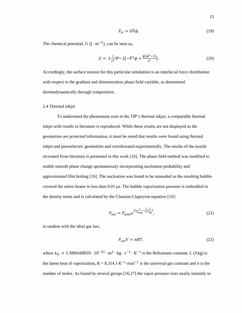
2.4 Thermal inkjet

inkjet with results in literature is reproduced. While these results are not displayed as the

geometries are protected information, it must be noted that results were found using thermal

inkjet and piezoelectric geometries and corroborated experimentally. The results of the nozzle

recreated from literature is presented in this work [16]. The phase field method was modified to

enable smooth phase change spontaneously incorporating nucleation probability and

approximated film boiling [16]. The nucleation was found to be unneeded as the resulting bubble

covered the entire heater in less than 0.01 s. The bubble vaporization pressure is embedded in

the density terms and is calculated by the Clausius-Clapeyron equation [16]:

, (21)

in tandem with the ideal gas law,

, (22)

where is the Boltzmann constant, L (J/kg) is

the latent heat of vaporization, R = 8.314 J· · is the universal gas constant and n is the

number of moles. As found by several groups [16,17] the vapor pressure rises nearly instantly to

16

roughly 10-13 MPa. This was corroborated by simulation as we achieved 12.1 MPa. To allow for

change of phase, the mass flux ( is evaluated from conductive heat flux,

. (23)

Here, is the molecular weight of the vapor (kg/mol) and is the enthalpy of vaporization

(J/mol). In making this approximation, one is neglecting the kinetic energies and work due to

viscous forces which slightly under predicts the mass flux. The problem remains to incorporate

this equation in a CFD format, accordingly one must define an expression for the rate of phase

change. The equation as seen above cannot be put into use as the peak temperature gradient

from the surface in question. Instead, the mass flux is approximated by,

. (24)

Mass flux found in bubble growth must be accounted for in the energy equation as well.

Accordingly, the energy equation becomes,

). (25)

Additionally, the equation for the phase field variable is modified to allow for the smooth change

of phase in respect to boiling or phase change,

. (26)

A known value for resistance is applied to the heater pad and a step input of voltage generates the

heating profile. Note: the results of this simulation cannot be displayed pictorially as it is an

experimental thermal inkjet and it is protected intellectual property.

17

CHAPTER 3. ANALYTICAL APPROACH

Three approaches were used in the understanding and modelling of the effects of the back

pressure initial condition on the jetting phenomena. The first two of these were based in

computational fluid dynamics and the third presents an analytical solution for droplet creation,

diameter, and velocity.

3.1 Simulation Details

Understanding the reasoning for the method by which the simulation techniques were

chosen lends itself to the understanding of the validity of the results for a given simulation. By

outlining the choices and reasons for these choices, the results are more readily understood. To

understand the phenomena seen in the thermal inkjet system, we examined the same phenomena

in a well-defined piezoelectric inkjet system. The primary method of demonstrating the effects of

modulated static contact angle is through the simulation of the piezoelectric inkjet, this was

chosen to be an acceptable method as the pressure pulses are of similar amplitude, length, and

originate from a similar location in the inkjet nozzle, in the following sections all other

assumptions used in the numerical simulations are explained and justified, this includes

physically accurate diffusion, phase change, mass conservation, and phase separation.

3.2 Simulation Method Selection

When utilizing computational fluid dynamics to gain insight into a phenomena, besides

benchmarking results against experiments, and previous simulations, there still remains the

18

choice between numerous computational schemes, each with several advantages and

disadvantages. There are three primary types of simulation used in CFD, moving mesh based,

level set, and phase field. The first to be considered is modified level set. It has several

advantages, such as capturing topological changes; easily finding intrinsic geometries. It is also

relatively easy to implement, has an accurate high-order computational model, and boasts

improved mass conservation, even slightly better than phase field. However, to contrast these,

there are several disadvantages. It is mildly non-conservative leading to loss or gain of mass

(area) due to numerical diffusion. Additionally, it is computationally expensive, and re-

initialization is needed to maintain the signed distance function. This is a function to determine

the distance of the center of a given element to a respective boundary, and the sign determining if

the point is within a given set. Another possible method for simulation that was considered was

the moving mesh based ALE (Arbitrary Lagrangian Eulerian). This method boasts many

excellent features and only a few extremely notable disadvantages. Some of its excellent

advantages are its ability to conserve mass and track the exact position of the fluid interface. The

method is usually preferred when maintaining an exact boundary for separating the phases is

paramount to the physics being modeled. However, it should be noted that as a result, auxiliary

physics can be modeled in either of the phases individually but not interacting.

There is an ease of introduction of auxiliary physics for independent phases (gaseous,

solid, and liquid). This is counteracted by the relatively severe disadvantages exhibited by the

method. An example of this is the phenomena found in a thermal inkjet. In this system, the

moving mesh method is inadequate to model interacting physics and diffusion across boundaries.

It is more computationally intensive, and is unable to compute topological changes, sharp corners,

and it has poor performance when applying surface tension as it must reconstruct the interface

from a discontinuous fun

19

step. Furthermore, the curvature of the interface is difficult to compute accurately using VOF

(Volume of Fluid) techniques. The method that was chosen was sharp interface phase field, which

has its own set of advantages and disadvantages. Its advantages suited themselves well to the

modelling of inkjet based phenomena as it can be coupled to various turbulence models, for

example the impingement of high speed liquid jets. The phase field model easily lends itself to

coupling with other computational physics, for example complex events such as film boiling. It is

computationally quick: 6 to 8 times faster than a modified level set computation of the same

numerical setup, with more intense meshing. It easily handles sharp interfacing, has better phase

change, physics coupling and structural interaction, and it is comparably accurate with more

intense meshing. It does have its disadvantages, as it is the least conservative modelling method

as a result of how the phase is smoothly varied. This causes it to be mildly less mass conservative

for similarly sized meshing when compared to modified level set due to an additional transport

equation. However, with sufficiently intense meshing, physically-validated results were achieved

faster than less accurate level set models with coarser meshing. It was chosen because it could

adequately model the selected physics and could create accurate mappings of jettability with

moderate computation speeds. Lastly, phase field allows for ease of transition of modelling

methods across simulated platforms, allowing for a similar approach to be used in piezoelectric,

induction coil based, and thermoelectric jetting

3.3 Analytical Model

To help predict the drop volume and speed within stable regions, we use an analytical

model to find velocity and accordingly, height, break off, and radius of the jet; this provides

approximate droplet volume. Approximating the droplet as a long cylinder, we can then

approximate the energy loss during flight as a result of transitions between oblate and prolate

phases.

20

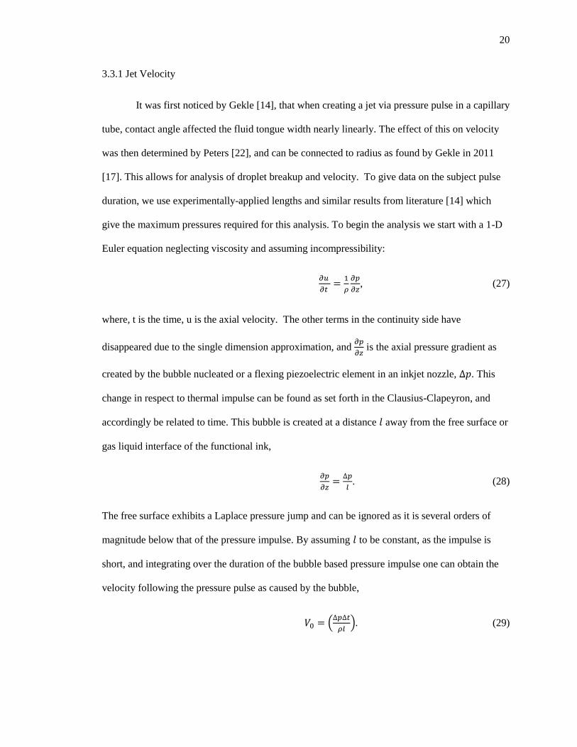
3.3.1 Jet Velocity

It was first noticed by Gekle [14], that when creating a jet via pressure pulse in a capillary

tube, contact angle affected the fluid tongue width nearly linearly. The effect of this on velocity

was then determined by Peters [22], and can be connected to radius as found by Gekle in 2011

[17]. This allows for analysis of droplet breakup and velocity. To give data on the subject pulse

duration, we use experimentally-applied lengths and similar results from literature [14] which

give the maximum pressures required for this analysis. To begin the analysis we start with a 1-D

Euler equation neglecting viscosity and assuming incompressibility:

, (27)

where, t is the time, u is the axial velocity. The other terms in the continuity side have

disappeared due to the single dimension approximation, and is the axial pressure gradient as

created by the bubble nucleated or a flexing piezoelectric element in an inkjet nozzle, . This

change in respect to thermal impulse can be found as set forth in the Clausius-Clapeyron, and

accordingly be related to time. This bubble is created at a distance away from the free surface or

gas liquid interface of the functional ink,

. (28)

The free surface exhibits a Laplace pressure jump and can be ignored as it is several orders of

magnitude below that of the pressure impulse. By assuming to be constant, as the impulse is

short, and integrating over the duration of the bubble based pressure impulse one can obtain the

velocity following the pressure pulse as caused by the bubble,

(29)

21

After there is a driving impulse, there is no more acceleration generated from a forcing

function. However, acceleration still takes place in the form of flow focusing due to the shape of

the free surface. As with the initial steps, the analysis follows the work of Peters [22].

Acceleration as created by the pressure impulse is based on the continuity of the fluid, so as a

result we start by assuming a free surface with a radius of curvature, , and the previously

mentioned one dimensional velocity. With flow rate constant, and dV defined as a small velocity

increase and dR as a small reduction in radius, one finds,

(30)

reduced to,

. (31)

The radius of curvature is expressed using the nozzle radius, , the contact angle, and applied

back pressure as shown by the Young Laplace equation. The equations above derive the radius of

curvature as illustrated earlier, allowing for one to generate the expression for acceleration,

(32)

Where the contact angle held was initially unforced outside of capillary action and gravitational

body forces, an additional pressure loading has been applied forcing the meniscus to bend until it

exceeds its receding contact angle, at which point the fluid retreats. From this it is easy to see that

smaller nozzles have stronger focusing as illustrated in the differing nature of experiment and

thermal inkjet CFD where the drop volume was easily reduced by a factor of 100 in a 67 micron

nozzle and simulation where it was only reduced by 10. It is at this point one has to determine

how long the fluid is additionally accelerated from this flow focusing,

. (33)

22

As a result the effects of focusing can be seen as,

. (34)

However, unlike acceleration, the velocity increase is not dependent on nozzle radii. As a result,

the velocity achieved by the fluid jet, in respect to a proportionality factor assumed

experimentally to be 2 as found by Isshiki is,

. (35)

It is at this point that as with Peters one can apply the needed corrections for the fact that the

pressure pulse is applied to a curved gas-liquid interface, approximate velocity distribution and

volume conservation to account for the curved interface when calculating the velocity of the fluid

tongue [22]. It is assumed that the tangential velocity components are negligible, thus only

normal velocities are used. With this assumption, one is allowed to consider the surface as an

isopotential region. Assuming the one-dimensional approximation, there is a uniform axial

velocity, with isopotential interfaces facing perpendicular to the walls of the nozzle. The gas-fluid

interface is defined as the curved meniscus, which is an isopotential surface that requires it be

matched to the planar isopotential region beneath it in the general fluid source in the nozzle. By

adding the distance, , the smallest length away from the interface where the assumed

isopotential regions are not affected by the curvature of the meniscus, Peters allows one to correct

for this, using it as a fitting parameter [22]. One can then find the distance between the meniscus

and the horizontal plane, normal to the fluids surface. This is based around the angle between

the normal and effective distance

(36)

23

Velocity is inversely related to this as the relation between the plane and free surface is constant.

To evaluate the mass flux through the region of the nozzle in the bulk fluid, one can use the fact

that the velocity is uniform and as mass is conserved it equals that through the fluid-gas interface.

Figure 4. Nozzle meniscus features and dimensions.

. (37)

Where , is a correction factor as found by Peters to be roughly unity at 0.94, the other correction

factor was found to be [22]. This yields (

. (38)

3.3.2 Jet Breakup and Radius

Integrating the velocity of the jet over time yields the height achieved by the jet. The

acceleration and velocity profiles in respect to the input of a pressure profile have also been

solved for. Accordingly, there remains the task of finding the jet radius and time to pinch off.

From this, one can obtain the total amount of fluid released from the fluid tongue. Jets break up

due to the growth of capillary perturbations in a cylindrical jet as shown by Gekle [18]. Surface

24

tension drives the growth of instabilities leading to eventual pinch off. In the unperturbed flow of

a jet, if , the time evolution of a jet radius is prescribed by the velocities in the ballistic

region, and can be found if one neglects surface tension and uses the thin film approximation.

Due to the thin nature of Worthington jets, thin film approximations give very physical results.

Using the velocity and acceleration values, the height and radius of the jet can be determined at

any given time step [18]. The momentum equation of Navier-Stokes along the axial path of the

fluid jet can be written as,

(39)

and the continuity as,

. (40)

The jet radius is found at a given height, if there is a complete set of knowledge pertaining to the

ballistic region, which has been derived in the previous section. A fluid particle being ejected

from the axial acceleration region into the ballistic region, at time will at any time, t, have

reached the height:

. (41)

These fluid particles are pushed from the axial acceleration region at unique times, accordingly, ,

is able to represent each fluid particle respectively. Integrating one can obtain,

. (42)

The strain rate for the ballistic transition is,

. (43)

25

This yields,

. (44)

The breakup of a jet is simply a response to the fact that fluid jets are inherently unstable, and in

order to minimize its energy state, a fluid column seeks the lowest possible surface area, which is

a droplet. The capillary perturbations create a wavy profile which grows until eventual pinch off,

this is known as Rayleigh break up and is demonstrated by Gekle [14] for jetting phenomena. The

perturbation that grows the quickest is responsible for the eventual pinch off and has a

wavelength of,

. (45)

The characteristic time describing the time till break up is the time scale as described by the

balance of the inertia,

, and capillary forces, , generates the capillary time scale,

. (46)

The jet breakup into droplets breaks up on a time order roughly equal to that of the capillary time.

The resulting droplet volume should be,

, (47)

=1.88 . (48)

26

3.3.3 Droplet Velocity

Figure 5. Left: prolate spheroid, Right: oblate, Mass coordinate diagrams: describe oscillatory phases of a moving droplet in free space.

The nature of Worthington and focused jets, generates an additional acceleration to the

fluid tongue. One might expect that this will generate a faster droplet. However, analytically and

experimentally this is not the case. Instead, a more complex relationship is found in which energy

is dissipated following breakup through viscous effects of oblate and prolate transitions. The

velocity of the focused jet generally exceeds that of the general fluid flow from an inkjet nozzle

sans focusing. While the extra acceleration is related to final velocity, it is not a simple relation.

Long

cylindrical columns of fluid to spheres, the longer and thinner the more they distribute energy per

unit mass. This is because the tip is of roughly equal mass to the non-moving tail, and in oblate

and prolate transitions it dissipates energy. This works in tandem with the momentum balance of

the droplet tip and tail. As the tail of a droplet is pulled up to join with the primary body of the

droplet, it further decelerates the thinner focused jets. The deceleration based on oblate-prolate

transitions and the pulling of the droplet tail can be lessened as the profile gets thin enough that it

pinches higher up, however the general effect follows the simple mathematics of a mass-spring-

dashpot system as stated by Einstein [15]. The droplets effectively shake themselves slower. To

analyze the effect, this may have on droplet flight, we start with the assumption of small

27

deviations from the spherical shape. We assume this only results in pressure loading on the

interior and surface potential flows. This formulation results in a polynomial expansion in regards

to the displacement field. This can be used in a series solution of the Navier-Stokes equations.

Accordingly, second-order differential equations describe the deformations in respect to the

modal displacement functions. This analysis was found and validated by Isshiki [20] as the

equations found are simply the logical expansion of the Rayleigh-Lamb theory in which is found

a non-dimensional representation of deflections on the time scale T = t/t*, where non-dimensional

time t* is

t* . (49)

With this non-dimensionalization, we can then find the equation with one additional assumption,

that the mode of deformation is that of a simple oblate-prolate form, this is heavily supported by

experimental results for an inkjet system as for them to have higher order forms the droplet must

have a Bond number far greater than 1, and all droplets recorded by all means of experiment,

simulation, and analytical result do not fit this criteria. The displacement of the relative stagnation

(m,) is assumed to be of order two accordingly. The Reynolds number for the following

calculations is assumed to be for internal flows,

. (50)

However, unlike the assumptions, the deformations found in inkjet droplets is relatively large so

we must further follow the modified theory for nonlinear deformation as seen in the analysis

performed by Schmehl [23]. The forces throughout and around any respective droplet are now

related to any given point of deformation. Additionally, minor nonlinear effects are brought about

with greater viscous stress in the droplets interior flow. The type of deviation that can be seen

from the linear behavior in the case of the inkjet droplets is a shifting oscillation frequency. In

28

this instance, shifting oscillation frequency is a dominant factor. Accordingly, to set up to solve

for this, we use an energy balance for the droplets with the reduced assumption , and

(N/( s)) is a dissipation function in respect to viscosity as previously derived [14]. For

spheroids (oblate, prolate, and spherical), the rate of surface area change can be calculated from

the implicit analytical expressions relating the change rate of surface area, S ( to the viscous

internal losses.

, (51)

(52)

Assuming that the droplet is in the shape of a cylinder initially, one can accordingly

assess the axial and radial motion on the surface of the droplet. To quantify deformation and

kinetic energy, the coordinates of mass as seen in the diagram, are used to show the

radial and axial translations of a droplets boundaries,

. (53)

. (54)

To find the term for dissipation in a drop, a function for dissipation is found in [14],

, (55)

. (56)

To find the energy dissipated one must evaluate:

29

(57)

Symmetry and general continuum assumptions allow for an assumed radial velocity gradient at

the axis, , and at the equator: , this gives the ability to evaluate the energy

dissipated. This yields the energy dissipated,

(58)

Recombining equations (59-66) yields the equation for the behavior of a falling droplet. Using the

initial conditions as previously solved for: jet velocity, pinch off, radii, and initial velocity, and

length, allows for numerically solving the above equation.

, (59)

yielding an approximate solution assuming stable droplet creation, and accordingly in the jettable

regions seen in the figures in Appendix B. Isshiki linearizes at this point in respect to the

dependent variable and set which results in,

. (60)

This yields,

. (61)

Applying the data as found in the earlier portions of analysis gives the kinematic response of the

travelling and distorted droplet, assuming drag to be negligible. This allows for ease of

calculation, and a reasonably accurate approximation of oscillation, dissipation and momentum

balance.

31

, u is its velocity ( ), L is the characteristic

). The parameters that

control the effects of back pressure are viscosity, surface tension, driving waveform, density,

refill dynamics, geometry, and nozzle size. The Bond number (Bo) is used to justify the accuracy

of these non-dimensional spaces as a Bond number greater than one indicates that the droplet is

too large for this form of analysis.

3.5 Model Assumptions, Selections, and Justifications

The selection method for a computational fluids methods aside, when applying a given

method many factors must be taken into account to ensure that the results of a given simulation

are physically accurate allowing for accurate predictions of physical phenomena. The method

used throughout this work is that of the phase field method. The phase field method uses a fixed

mesh and computationally is configured as a single fluid of differing properties spatially. The

interface in the phase field method is considered to be of a small but finite thickness in which the

two immiscible phases are miscible as seen in their diagram, giving a smooth variation of fluid

properties in the computational space. This type of phase transitional phase is referred to as

spinodal decomposition, and is due to the miscibility gap in the phase diagram. Accordingly, the

start of phase separation occurs when a given fluid transitions into its unstable portion of the

phase diagram with respect to the free energy balance of the two chemicals as found using the

particle concentration and the free energy of the respective homogenous solution. The boundary

of the unstable region is sometimes referred to as the binodal region. When transitioning through

the spinodal and binodal regions, the phases are seen to separate via a generalized diffusion. This

via diffusion, there often is a negative diffus

unphysical approximation of this phenomena. To separate the two immiscible phases it is

32

-

Hilliard equation. The Cahn-Hilliard equation governs the separation of two species in the

spinodal region and can be derived using kinetic theory. The pseudo stable phase region is found

at the local minima, and not the global minima of free energy as proposed by Gibbs, and is

resistant to fluctuations of inverse proportions in magnitude and scale. It is this method that tracks

the interface of the two fluids in the multiphase flow. Comparing a portion of the Cahn-Hilliard

equation yields the similarity one might expect,

, (67)

. (68)

Surface tension is also found in respect to Gibbs free surface energy. Accordingly, surface

tension is derived thermodynamically as seen in the balance of entropy and enthalpy of the fluid-

gas interface. This is physically well accounted for in the phase field method as the mixing

energy density over the interface thickness is the driving factor of surface tension. The

assumption for interface thickness is based upon the equilibrium solution of the Cahn-Hilliard

equation. To justify this assumption, Boley in 2013 [5] demonstrated the equil

second law, this can be extended to the Cahn-Hilliard equation as well. Additionally, all methods

were examined against a physical system and the results compared yielded similar results.

Validating the assumption of equilibrium conditions is the evaporation rate of the first drop being

governed by the diffusion of the liquid vapor in a gaseous medium. This is completed in two

distinct ways. The first step is to find the vapor transport induced by natural convection, and

show the result of this to be effectively negligible. Boley [5] examined the effects of natural

convection on evaporating sessile drops. An empirical model for combined diffusive and

33

naturally convective vapor transport can be used. From the model presented, the convective vapor

transport contribution can be neglected if,

. (69)

Substituting values used experimentally and computationally, results in values ranging

from 0.02-0.16 for the left hand side of the above equation. This falls primarily within the

reported uncertainty range (±0.08) found in [5]. This result when coupled with the fact that in [5]

the effect of natural convection on small evaporating sessile drops is negligible. This allows for

one to propose neglecting mass transfer by natural convection terms. The second step in this

[5]. This condens

for the vapor concentration as shown by Boley, using previous arguments found in literature.

Specifically, by compared time scale of mass transfer of the vapor through the interface and the

time scale of diffusive relaxation of the layer saturated vapor interface. Boley reported that the

ratio of the time required for the vapor concentration to adapt to changes in fluid interface

shaping to the time required for the drop to fully evaporate by diffusion is on the order of

1. Using this approximation is a conservative approach lending further

accuracy to the assumption of a metastable equilibrium condition on diffusivity as the mole

fraction of the ink solvent approaches 0 during the evaporation process while the specific volume

of the ink has a non-zero lower bound, the specific volume of the solute. Accordingly, one can

safely make the assumption of evaporation being primarily based in diffusion mechanics in the

vapor region surrounding the fluid-gas interface. This allows for one to easily use the assumed

interface thickness in the Cahn-Hilliard equation. Throughout this work, there are several

instances where nozzles and droplets of differing sizes by orders of magnitude are compared. For

this to be valid one must take into account spreading differences, evaporation rates, Bond

numbers, etc. To allow for these comparisons, the assumptions for these must be justified. The

34

Bond number for all works presented ranged from 0.001-0.09 , this allows for one to neglect

the overall effects of body forces on droplet creation and sessile droplet formation. The

assumption that the fluids created as a solution of particulate are ideal solutions and Newtonian

fluids was utilized to express the specific volume and the properties of the ink linearly, according

to the proportions of the solute in the solvent. Additionally, this can be used to scale, , by

the mole fraction. This assumption is not fully substantiated. Thorough analysis was not

conducted to validate the assumption that the inks of this nature can be approximated as an ideal

solutions. However, it has been shown that no solutes have been visible whilst holding the ink to

light throughout a period of up to 2.5 years.

35

CHAPTER 4. EXPERIMENTAL DETAILS

4.1 System

All physical experiments were performed with a HP TIPS system with a nozzle diameter

of 67 , with a voltage input of 29 V with a pulse width of 3.1 . The back pressure for all

data points was recorded via an internal pressure sensor in the TIPS controller at the instance of

each firing, and the control of pressure was achieved through the use of a syringe. The nozzle is

primed before the printing of any pattern by forcing a small amount of fluid out of the nozzle

using the syringe then pulling back any excess then wiping the print head clean of any remnants.

The Pd ink and SU-8 underwent the same waveforms and procedures for all tests. A minimum

temperature and maximum temperature of 22 and 26 degrees Celsius was held throughout all

printings.

36

Figure 6. A) Experimental setup, B) and generic nozzle profile of TIPS nozzle image (Not able to disclose HP intellectual property, all thermal inkjet results are additionally not released),

scale withheld and image distorted.

4.2 Drop Volume Experiments

To find the average mass of the droplet, 432,000 droplets were deposited on a pre-

weighed piece of aluminum foil and allowed to dry for 24 hrs in 60 layers of a 60 by 120 dot

matrix. A single nozzle with a slow firing frequency of 1000 Hz was used to avoid cross talk;

however, slower than this could promote clogging, and as such the long period of printing could

be prone to failure-to-fire events. Additionally, this process was watched continuously for trends

or clogging. The results of these experiments were then measured. Using the fluid properties and

concentrations one can then obtain data on the droplet volume.

4.3 Drop Speed Experiments

To find the droplet velocity, we utilized the method of bidirectional printing with varied

heights [5]. This test consisted of multiple single column target print patterns, printed bi-

directionally at high scanning speeds, , with known stando distances between the print

droplet impacted on the substrate, as there is a understood time delay as the droplet must travel

37

between the nozzle and the substrate. The result of this is the actual deposition position of every

droplet had either some translation correlating to the lead or lag and the true trigger position

depending on the print scan direction as seen in Figure 9.D. The distance, d, between the two

columns of dots was found by subtracting the centroid positions of the drops in each column

through image processing algorithms in MATLAB using a circular Hough transform. The time

combination using these

images,

, (70)

where was the highest stage speed of 225 mm/s and the stand-off distances ranged between

0.3 mm and 2.1 mm. Assuming drop speed changes minimally throughout the flight time, the

impact velocity is the slope of delay against standoff distance. This also served as a method for

satellite detection, as the high stand-off distance and speeds would exacerbate satellite trajectory

differences and increase offset on the substrate. To examine the possibility of a frequency of fire

limiting phenomena, we simply attempted to print patterns on parafilm with as tight a pixel pitch

as possible while using the maximum speed of the stage, . This gave the ability to check for

fire while refilling or failure to fire visually via qualitative checks between speeds, at a set back

pressure. Visual recognition code recognizes satellites and reports their size, number, and their

respective centroids using similar methods.

38

Figure 7. This figure depicts a recreation of Castrejón-Pita in 2011 [6] and adaptations of his simulations as performed in COMSOL. In Figure 7.A, an automesher was utilized to create the initial mesh and the setting extremely fine physics based meshing was

applied. In this setting, lagrangian-based meshing with an initially even distribution of elements is created. The initial number of elements was 432,000. However, an adaptive meshing scheme was applied so this changed the number of elements to increase accuracy based upon the movement of

the fluid-fluid interface, In Figure 7.B, Velocity input waveform [7], In Figure 7.C, Diagram of simulation properties.

39

The results of the original experiment and simulation were first found through fine tuning

of the system while using phase field methods, this result was then used to verify the accuracy of

the simulation. DOD (Droplet on Demand) droplet formation for a glycerol-water mixture was

simulated and compared with the results obtained by Castrejón-Pita in 2011 [6], where the

density, viscosity, and surface tension of the glycerol-water mixture are ,

, and 0.064 N , respectively. Back pressure was then applied to two levels with an

assumed receding contact angle of 5 degrees to obtain a clear trend. The droplet is examined for

speed, volume, and satellites, then lands on a piece of glass and is examined. There was use of up

to 40% adjustment in the driving forms amplitude and this was tuned to achieve the closest results

possible. All meshing was automatically done using the tightest physics based meshing.

The back pressure is applied for 40 milliseconds for pseudo-equilibrium, the meniscus is

nearly static, at which point the waveform is applied to the inlet at which point the droplet is

ejected traditionally. This numerical experiment is performed for a variety of fluid properties. In

Figure 2, boundary conditions and applied meshing, piezoelectric waveform as found

experimentally [7].

40

CHAPTER 5. RESULTS

To experimentally investigate the phenomena connecting back pressure modulation and

droplet volume and velocity, two relatively differing fluids were jetted and observed, as seen in

Figure 8. The fluids were SU-8 2002 and Palladium hexadecane thiolate ink (Pd ink) with a

concentration of 47400 in toluene. In the case of the Pd ink, by using the average drop

mass measurement one can obtain a maximum average droplet diameter of 65.18 and an

average minimum of 25 at average pressures of 287 Pa and 9247 Pa respectively. Additional

tests for SU-8 2002 yielded similar results as the diameter decreased in a nearly linear fashion

with higher back pressure creating satellites. Nonlinear effects of velocity and drop volume are

seen in the results of SU-8 2002 and are described by the change in pinch off time being affected

by the growth profile of the jet changing the aspect ratio of the resulting droplet. The pinch off

point changes the drop volume directly, and the change in droplet speed is a result of manipulated

contact angle creating longer more cylindrical droplets.

5.1 Experimental Methods

To compare these to the apparent diameter of the droplets deposited optically, we assume

the droplet formed with no back pressure to have a diameter comparable to that of the nozzle

preceding impact. We then determined the diameter based upon wetting dynamics and capillary

spreading being of a longer time scales than the initial spreading and contractions and shorter

than evaporation [5]. A droplet of Pd ink with a back pressure of 750 Pa has a diameter of

roughly 28 [11]. Similar results were found with all other inks and using several nozzles of

41

the same type, this is shown in Figure 8. Back pressures for SU-8 are only shown from 8.3 Pa to

583.33 Pa. This is because satellites are formed from 583.33 Pa through 708.33 Pa for the same

driving waveform as used for the Pd ink. By reducing the input waveform amplitude from 29 V to

28.92 V stable droplets could be created. This is because a larger voltage created a larger pressure

spike which ejects too much fluid in a long thin cylinder allowing for a higher Rayleigh

waveform number causing for multiple breakup points. In experiments using Pd ink, a back

pressure of 875 Pa would yield satellite droplets similarly to SU-8. A reduction in voltage from

29 V to 28.92 V yielded fully stable droplets when printing patterns at 1 kHz. Further reduction

of voltage input lead to a situation where unstable droplets were not creatable but rather a no fire

event was reached. This stands to support simulation results, and demonstrates a considerable

range increase from that of a square wave input. When evaluating results, it must be noted [21]

that there is a relatively dissimilar Bond number; however, both are found to be less than one. To

compare two dissimilar methods static initial condition manipulation and dynamic manipulation

through applied waveform, we assume the contact angle to be that found right before a forward

impulse. This means that the shape of the fluid-air interface is the same exact shape for both

systems regardless of how it was achieved.

42

Figure 8. The data points compare all previous literature with the data from this work. The experimental results are compared and contrasted with work by Basaran [9],

analytical results, and computational methods. In these figures all experimental data points are color. They are depicted in relation to receding contact angle and back

pressure. In these figures cyan represents SU-8 2002 experimental results, whereas, black, represents toluene based inks experimental results. In regards to other works

Triangles represent analytical solutions for toluene based inks, diamonds represent CFD results for toluene based inks, and additionally for reference data,

presented as red diamonds.

43

Drop volume decreases nearly linearly with increased back pressure. (Note: in Figure 8 of

droplet deposited show what appears to be splash marks in photos of palladium ink, while

possibly splashing, these have previously been found to be a result of the drop morphology of

larger droplets due to Marangoni flows being stronger in the larger volume of fluid, these

accordingly get smaller as the droplet gets smaller reducing the effect [4]). Droplets shown in

figure 8 were found to be close to the statistical average diameter as deposited on polished

silicon, SU-8 2002 tends to polymerize during flight at increasing rates and times as the drop

volume decreases and length increases, respectively this rendered comparison between deposited

droplets and droplets in flight difficult as the spreading dynamics are subject to change in respect

to height of deposition and size and as such are all shown from the lowest height of 0.3 mm.

Additionally, droplet deposition was unsustainable as there was leaking and clogging at back

pressures below 1000 Pa and are accordingly not represented. Lastly, a trend in droplet

production was that upon incurring satellites the fluid volume ejected is reduced, including

satellites, again as the upswing is reversed this is reflected in dot gain of the primary droplet.

44

Figure 9. (A) Toluene: blue: SU-8: green: Comparison to printable region diagram [8], (B) Reynolds vs. Ohnesorge Reynolds numbers, comparison to printable region diagram[10], (C)

comparison to printable region diagram [21], (D) I. Frequency to fire at back pressure 750 Pa, standoff distance of 0.6 mm, firing waveform 29 V with duration of 3.1 : I. 100 Hz firing

frequency with Pd in with a back pressure of 750 Pa, II. 100 Hz firing frequency with SU-8 2002 with a back pressure of 500 Pa, III. 2000 Hz firing frequency with Pd ink with a back pressure of

750 Pa, IV. 1500 Hz firing frequency with SU-8 2002 with a back pressure of 500 Pa.

5.2 Simulation

Simulations gave a qualitative and quantitative approach towards determining the effects

of back pressure. The primary effect can be seen as three distinct effects working in conjunction

to reduce drop volume. The first effect is that the energy to eject the droplet increases as the size

of the meniscus increases, a reduction in input energy decreases droplet volume linearly to a point

[16]. In practice, this marginally narrows the profile and suppresses the expansion of the droplet.

However, the nature of the effect of back pressure on drop volume is based on the suppression of

droplet growth along the sides due to inertia of the fluid in the meniscus and the collapse of the

meniscus. As such, the other effect that further exacerbates this reduction in volume is the

horizontal collapse of the meniscus due to channeling of the fluid along the angled sides causing

the formation of a Worthington jet [8]. This causes a sharp profiled jet to protrude from the

45

already narrowed column of fluid. A sharper angle would incur a more aggressive collapse. As

the meniscus acts to narrow the jet, we achieve an almost sharp and pointed profile, and this

profile then continues to expand. This jet then becomes unstable and breaks up leaving a droplet

far smaller in diameter than the nozzle. Lastly, the fluid must move through additional space to

exit the nozzle and accordingly is not given the same amount of time to grow and lengthen before

the refill oscillations begin. This reduces aspect ratio of the column ejected and showed attributes

similar in nature to those previously expressed [2, 8].

46

Figure 10. Simulation confirmation, applied waveforms, applied back pressures, geometry, 1st row results compared [7], 2nd and 3rd row illustrate effects of back pressure using the same waveform as found by Castrejón-Pita [7] and as seen in the 0 Pa row above, 4th row illustrates

modified waveform, waveform 1 as seen in experimental setup. Numerically it was determined that the drop diameter for the simulation of this waveform with no back pressure was 2.158 mm. However, with a back pressure of 70 Pa the diameter was reduced by 4% to 1.38 mm accordingly the drop volume was reduced by 74.9%. Additionally, when the modified waveform was applied the droplet diameter was further reduced by 52.5% to 1.05 mm and droplet volume decreased by

86.6%.

47

The results when comparing analytical, experiment and simulation are generally good as

they align themselves with experimental results as well as expected correlation with previous

works and natural phenomena, however there are some dissimilarities that must be accounted for

when examining their differences. The first difference that must be confronted is regarding the

method that one might safely assume to be the most accurate, computational fluid dynamics. In

this method, the reasons for the differences between computational and experimental results are

noise, mild material property differences, and geometry dissimilarities. Furthermore, the

simulation model of boiling is a known approximation with predictable and known shortcomings.

There are approximations made that under predict mass change and accordingly the pressure

pulse, accordingly the droplet speed and size is slightly smaller. More specifically, the

approximate expression for the rate of vapor generation is widely understood to result in a rate of

simulated vaporization that is lower than expected experimentally. Additionally, the isotropic

artificial heat diffusion, as found in the heat transfer equation, causes a higher than is physical

transport of energy from the boundaries to the vapor surface. This results in an unphysical rate of

bubble growth and vaporization. The solution becomes mesh dependent. Lastly, the model fails

to acknowledge radiation transfer from the hot surface to the liquid interface. The analytical

model is excellent for well-behaved, thinner fluids, with very slow pressure drop, as it over

refill

oscillations. It relies on capillary deceleration as its only means of slowing the jet. When

attempting to apply these mathematics to the refill period they fall short as the negative

accelerations no longer can apply to the same set of equations as derived for velocity. However, if

one imposes the refill oscillation parametrically as a mass-spring-damper, understanding that the

equations for pressure s effects on velocity are not nearly as accurate and this develops a

reasonable facsimile to the experimental data.

5.3 Frequency Stability

48

Throughput is always a primary concern when evaluating functional inkjet printing. For

the TIPS 23, the maximum firing frequency for de-ionized water is 4 kHz, however, the

suggested frequency for all fluids is less than 2 kHz as this prevents fire during refill as well as

the coincidental heating of the die which can degrade functional inks and change fluid properties

considerably. Accordingly, we tested the system at a maximum frequency with Pd ink in toluene

achieving a maximum firing frequency, as restricted by spacing and stage velocity, of 1184.21 Hz

and 2045 Hz at 100 Pa and 750 Pa respectively with minimal degradation of quality, no satellites,

and no observed failure to fire events, when compared to lower frequencies. This method

produces a similar range in stable droplets to that seen in Castrejón- 012 [7] within

2 kHz firing frequency. While there is an intuitive reduction in refill speed with increased back

pressure, this data shows that the effect of high back pressure does not significantly reduce the

maximum firing frequency as other factors such as, die heating or droplet morphologies that may

restrict it first. Additionally, all alternative piezoelectric pressure waveforms used to reduce

droplet size involve a preconditioning negative impulse that is then either removed allowing for

collapse [8] or a positive impulse is sent forcibly collapsing the meniscus [9]. This type of

waveform also decreases maximum frequency of fire in all inkjet systems.

5.4 Parameter Sweep Based Studies

To allow for comparison of all acquired data points both simulations, experimental, and

analytical, as they are not all of the same length scale, simulation reproduces both previous work

on a large, piezoelectric 2 mm, nozzle and the experimental 67 micron thermoelectric nozzle with

which experiments and simulations were performed. As a result, it is essential that it be presented

in respect to contact angle and back pressure. This emphasizes the importance of contact angle in

the jetting phenomena. All fluids were assumed to have a receding contact angle of 5 degrees as

that was assumed attainable with most fluids with proper surface conditioning. A parameter

49

ids as created to

facilitate a thorough mapping of the jetting phenomena in respect to several back pressures

(Appendix: A). The parameters involved in the sweep were that of density, surface tension,

viscosity, and applied back pressure. All remaining information involving droplet speed, mass,

and fluid contact angle was obtained through simulation results and the Young-Laplace equation

accordingly. These results were plotted in several ways until a cohesive region became obvious

to a skilled practitioner. It must be emphasized that the influence of nozzle geometry has not been

accounted for in this study and appears to play a large part in flow focusing and Worthington jet

based phenomena. As a result, some discrepancies between jettability should not come as a

surprise, as the formation of droplets is influenced by this as well, and geometry differs between

all respective nozzles. However, with that addressed, the phenomena presented in this paper

should be similar as long as the taper of the nozzle remains less than 45 degrees. As the taper

begins to exceed this, the phenomena becomes more and more collapse based and becomes better

understood in consideration of Worthington jet based mechanics [8].

5.5 Jettability Regions

To understand the evolution of jettability in respect to the change of a given parameter,

the number of pertinent factors must be reduced to three. Several previous authors have reduced

the number of fluid based variables in their own respective ways [8, 10, 21], and utilizing

different non-dimensionalization variables from the Capillary number to the Reynolds and Weber

number. The particular method used in this document is Reynolds vs. Ohnesorge on a log-log

scaling. This was chosen because of its obvious adherence to stability based guidelines as

described by Derby [13]. All jettability maps will be superimposed over all previous works to

give reference to previous guidelines for stability. The stability diagram used is similar to that

seen in Figure 5.B and is a recreation of the figure of the proposed jettability range by Castrejón-

50

Pita in 2012 [7] overlaid on the guidelines set by Derby in 2003. This indicates that meniscus

focused jetting primarily shifts the stability through the satellite droplets region. When using back

pressure there are many pitfalls. An excellent example of this is satellites can be created

preceding the bulk of the fluid. Satellites can also be found more traditionally following the bulk

of the fluid. This technique can also cause satellites in generally stable fluid and nozzle

configurations. However, despite these potential failure modes, the initial reduction in droplet

volume is almost always linear and stable. Some fluids seem to exhibit a completely linear

correlation in drop volume and velocity reduction in response to back pressure. Traditionally,

unstable fluids for a given nozzle can be made more stable through this technique. The

Worthington jet has a narrowed profile in contrast to normal droplet formations this drives fast

pinch off of small portions of narrowed jets, and accordingly less fluid, and smaller droplets.

In contrast to the general geometry of the Worthington jet, the jet tip region is increased

due to change in the push-pull dynamics and gravity assist. A thin column yields less fluid and

smaller droplets, but this can create satellites. Balance must be struck for each individual system

and fluid. Additional balancing is needed in light of the method of jetting being observed in

respect to the geometry of a given nozzle, as this will determine stability regions and transitions

between them. The first region for stable droplet was proposed by Derby in 2003 and has since

been primarily validated by many following works.

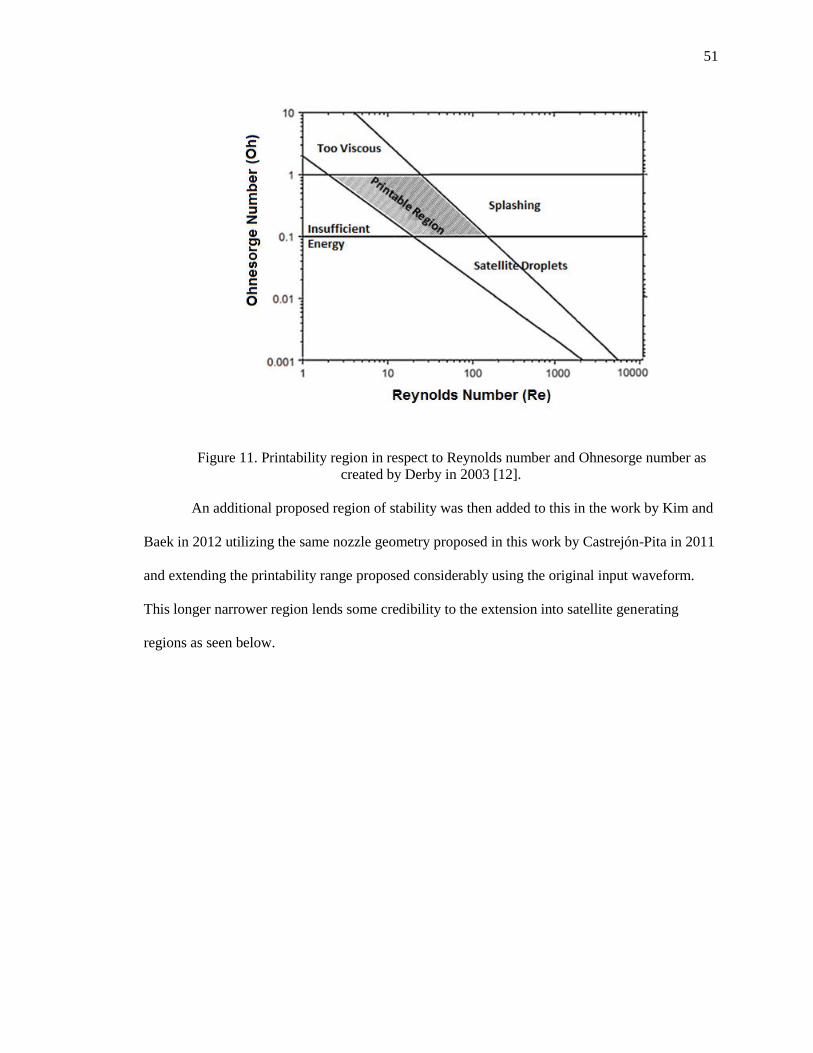
51

Figure 11. Printability region in respect to Reynolds number and Ohnesorge number as created by Derby in 2003 [12].

An additional proposed region of stability was then added to this in the work by Kim and

Baek in 2012 utilizing the same nozzle geometry proposed in this work by Castrejón-Pita in 2011

and extending the printability range proposed considerably using the original input waveform.

This longer narrower region lends some credibility to the extension into satellite generating

regions as seen below.

52

.

Figure 12. Printability region in respect to Reynolds number and Ohnesorge number as created by Kim and Baek [21] [12].

While Basaran was the first to notice the focusing behavior in respect to a negative pulse

followed by a positive in an applied waveform, Castrejón-Pita was the first to explore effects of

this kind and develop a parameter region was developed through the use of several nozzles of

extreme taper angles ranging from 45 to 90 degrees. This difference in nozzle geometry may be

the cause of the differences between the regions of stability seen in [7] and explored in this work,

as the primary factor in droplet is meniscus collapse in [7]. Whereas, shallower taper angles, as

seen in this work and Basaran s [1] demonstrate that flow focusing through the meniscus

dominates collapse dynamics in the formation of a jet and eventual droplet formation

53

Figure 13. Printability region in respect to Reynolds number and Ohnesorge number as created Castrejón-Pita in 2013 overlaid on the work found in [8, 12,17, 21].

Overlaying them all and generating a key allows for the evaluation of the evolution of the

printability regime.

The region found using the same nozzle geometry as Castrejón-Pita in 2011 with a

contact angle of 90 degrees generally corroborates previous works, although suggesting some

mild inaccuracies or discrepancies in the models, either modelling techniques applied such as

conservative phase field vs. moving mesh, etc. or geometry based differences. Regardless, the

model presented in this work seems to be slightly more generous in regions of stability as seen

below, at 90 degrees contact angle.

54

Figure 14. Printability region as found in literature with key for additional regions as seen below in respect Reynolds number and Ohnesorge number as overlaid on the work found in [8,

10, 21].

Applying a higher back pressure, we create a smaller contact angle and as we move the

static meniscus we see a change in the focusing phenomena as illustrated experimentally,

analytically, and computationally. This moves the stability region predicted down into the region

indicated by Derby to have satellite formation.

55

Figure 15. Printability region as found in literature with key for additional regions as seen below in respect to Reynolds number and Ohnesorge number as overlaid on the work found in [8,

10, 21].

Applying an even higher back pressure, we create a smaller contact angle and as we

move the static meniscus we see a progressive change in the focusing phenomena.

56

Figure 16. Printability region as found in literature with key for additional regions as seen below in respect to Reynolds number and Ohnesorge number as overlaid on the work found in [8,

10, 21].

Further application of back pressure yields the maximum deflection possible with the

given receding contact angle.

57

Figure 17. Printability region as found in literature with key for additional regions as seen below in respect to Reynolds number and Ohnesorge number as overlaid on the work found in [8,

10, 21].

Observing the possible implications of a contact angle over 90 degrees a 130 degree

- , which allows for a mild extension of the

printability region.

58

Figure 18. Printability region as found in literature with key for additional regions as seen below in respect to Reynolds number and Ohnesorge number as overlaid on the work found in [8,

10, 21].

The importance of contact angle as opposed to pressure can easily be seen in the

evolution of stability. Inertial terms and differing surface tension make certain fluids retreat either

too slowly in the case of dynamic manipulation, or retreat in the case of static application. This

causes certain data points to remain stable misleading one in the understanding of the phenomena

controlling jetting, or being lost as the fluid retreats back into the reservoir.

59

Figure 19. Printability region as found in literature with key for additional regions as seen below in respect to Reynolds number and Ohnesorge number as overlaid on the work found in [8,

10, 21].

Initially the results are strikingly similar between contact angle based regions and back

pressure.

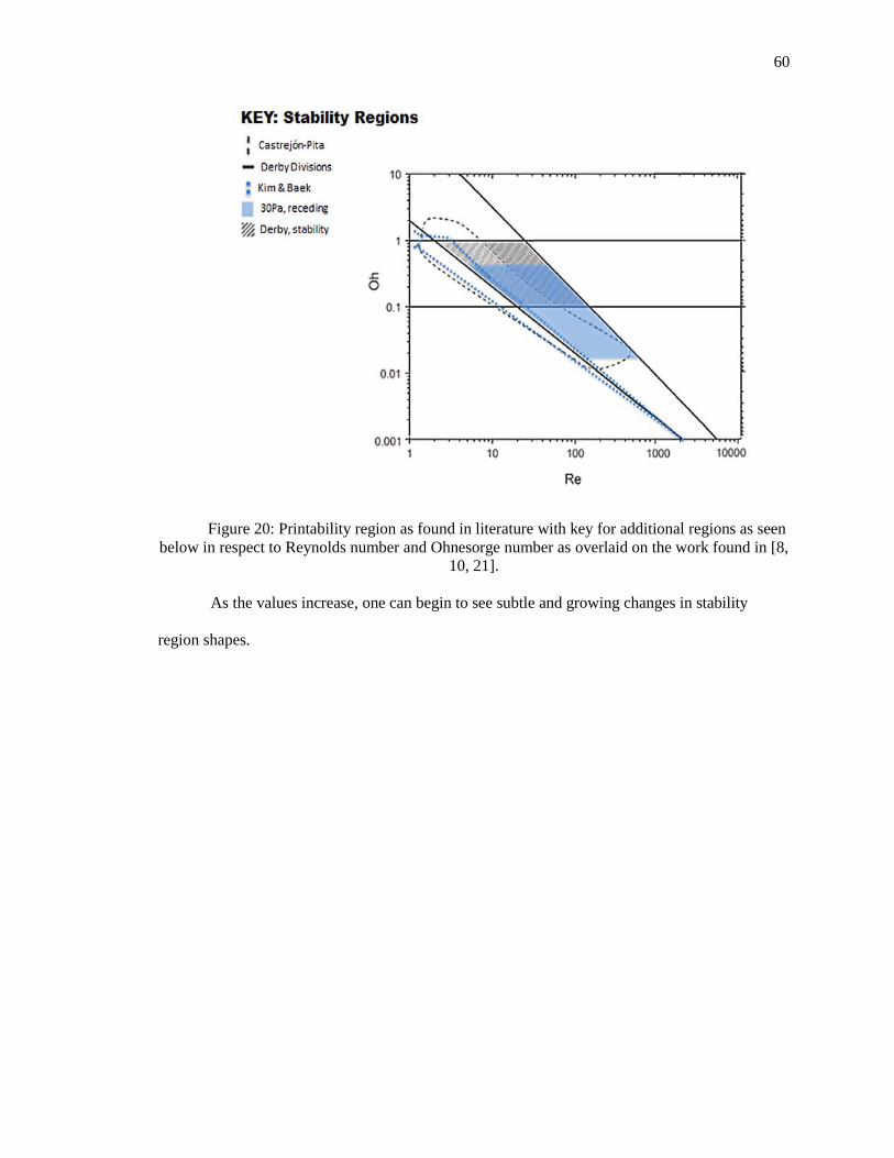
60

Figure 20: Printability region as found in literature with key for additional regions as seen below in respect to Reynolds number and Ohnesorge number as overlaid on the work found in [8,

10, 21].

As the values increase, one can begin to see subtle and growing changes in stability

region shapes.

61

Figure 21. Printability region as found in literature with key for additional regions as seen below in respect to Reynolds number and Ohnesorge number as overlaid on the work found in [8,

10, 21].

62

Figure 22. Printability region as found in literature with key for additional regions as seen below in respect to Reynolds number and Ohnesorge number as overlaid on the work found in [8,

10, 21]. Throughout much of literature there are several mappings of jettability and single droplet

stability. The mapping as used by Castrejón-Pita was selected as the Ohnesorge number and

Reynolds number on a log-log scale provides a clean region and large region that is relatively

linear in nature and can fit all behavioral models [8, 10, 21]. The importance of the contact angle

can be seen by comparing the evolution of the mapping as many fluids have begun to recede into

the reservoir well before reaching the maximum back pressure reducing the mapping. The

mapping in respect to back pressure, taking into account changing fluid properties and contact

angle hysteresis largely matches with prior work, however, when evaluating the results in respect

to contact angle the results become far clearer in respect to both theory and the evolution of

printability. This is due to the fact that receding contact angle, and inertial terms may also

contribute to the unclear evolution of the focusing trend. Additionally, all methods utilizing jet

63

focusing by manipulating the meniscus are heavily tied to the receding contact angle of any given

fluid and nozzle combination. However, unlike static back pressure methods, dynamic waveforms

merely begin to fail to show any results as the level of all fluid merely rises rather than creating

the meniscus curvature needed for flow focusing or collapse based jetting. This yields the likely

reason for why the results of this study yield a larger printability region than previous

experimental studies. Additionally, as with the receding contact angle all contact angle hysteresis

must play a larger part in the modelling of inkjet based phenomena as the advancing contact angle

plays a part in all positive back-pressure-based jetting and likely far more.

64

CHAPTER 6. CONCLUSION

Throughput, small feature size, and increased printing range are paramount in the world

of functional printing. Back pressure-based meniscus manipulation allows for potential increase

in performance in all three of these factors. While there exists several methods in literature that

can accomplish these improvements, they are not implementable across several types of printing,

specifically thermal inkjet. The effect is primarily driven by three factors: meniscus size,

geometry, and waveform. While other factors play into droplet modulation, such as fluid

properties and rheology, it is these three factors that can, in certain fluid systems, reduce drop size

and increase the printing ranges with regards to fluid properties, size, and velocity. Through

appropriate control of these factors, it is possible to tune the back pressure, passively or actively

to achieve smaller sizes from larger nozzles. As a result, one might be able to change print mask

designs for increased efficiency, and deposit fluids at speeds and in sizes potentially unreachable

by traditional methods of printing. Additionally, through proper contact angle hysteresis for a

given nozzle and geometry, the method of back pressure control is potentially usable across

platforms. This allows for ease of incorporation of this technique. Active back pressure control is

a practical, effective, and inclusive method by which one can modulate drop size and velocity and

increase printability range in a variety of fluids when using inkjet system.

LIST OF REFERENCES

65

LIST OF REFERENCES

[1] Alvin, U. and Basaran, O.

without reducing nozzle radius in drop-on- ., Physics of Fluids,

2002

[2] Bhuvana, T., Boley, W., Radha, B., Hines, B., Chiu, G., Fisher, T.S. "Inkjet Printing of

Palladium Alkanethiolates for Facile Fabrication of Metal Interconnects and SERS

Substrates." Micro & Nano Letters, Vol. 5, Iss. 5, pp. 296-299, 2010.

[3] Boley, W., Bhuvana, T., Hines B., Sayer. R.A., Chiu, G., Fisher, T.S., Bergstrom, D.,

Reifenberger, R., and Kulkarni, G.U. "Inkjet Printing Involving Palladium

Alkanethiolates and Carbon Nanotubes Functionalized with Single-Strand DNA," in the

Proceedings of the DF2009: Digital Fabrication Processes Conference, September 20-24,

2009

[4] Boley, J. W., Shou, C., McCarthy, P., Fisher, T., and. Chiu, G. T.-C, "The Role of

Coalescence in Inkjet Printing Functional Films: An Experimental Study" in the

Proceedings of the DF/NIP29 the International Conference on Digital Printing

Technologies, 2013.

[5] Boley, J. W. (2013). , Purdue University.

[6] Castrejón-Pita, J. R., Morrison, N. F., Harlen, O. G., Martin, G. D., and Hutchings, I. M.

angian simulations on the formation of droplets in drop-on-

demand , Phys. Rev. E 83, 2011

66

[7] Castrejón-Pita, A. A. and Castrejón-

[8] Chen, A. U. and Basaran, O. ius

without reducing nozzle radius in drop-on-

14, 2002

[9] Chen, P., Chen, W., Ding, P., Chang, S.H.

No. 1, Sec. 4, Roosevelt Rd., Taipei, Taiwan, International Journal of Heat and Fluid

Flow, 1998

[10] -2550. In Journal of the

European Ceramic Society 31, (2011)

[11] Derby, B.

Requirements, Fe

Vol. 40: 395 -414 (Volume publication date June 2010)

[12] Derby, B. and Reis, N. Inkjet Printing of Highly Loaded Particulate Suspensions. MRS

Bulletin, 28, 2003

[13] Derby, B., "Inkjet printing of functional and structural materials - fluid property

-414.

[14] Deserno, M. -Planck-Institut

FurÄ Polymerforschung, Ackermannweg 10, 55128 Mainz, Germany, 2004

[15] Einstein, A. (1906). "Eine neue Bestimmung der Moleküldimensionen". Annalen der

Physik 19 (2): 289.

[16] Fakhfouri V., N. Cantale, G. Mermoud, J. Y. Kim, D. Boiko, E. Charbon, A. Martinoli,

and J. -8 for polymer-based mems a case study for

67

[17] Gekle, S. and Gordillo, J. M. 2011 Compressible air flow through a collapsing liquid

cavity. Intl J. Numer. Meth. Fluids 67, 1456 1469.

[18] Gekle, S., and Gordillo, J. M., VAN DER MEER, D. & LOHSE, D. 2009 High-speed jet

formation after solid object impact. Phys. Rev. Lett. 102, 034502.

[19] Gordillo, J. M. and Gekle, S. 2010 Generation and breakup of Worthington jets after

cavity collapse. Part 2. Tip breakup of stretched jets. J. Fluid Mech. 663, 331 346.

[20] Isshiki. N., Theoretical and Experimental Study on Atomization of Liquid Drop in High

Speed Gas Stream. Technical Report 35, Transportation Technical Research Institute,

1959.

[21] Kim, E. and Baek, J. study on the effects of non-dimensional parameters on

drop-on-demand droplet formation dynamics and printability range in the up-scaled

4-present), 24, (2012)

[22] Peters, I., Tagawa, Y., Oudalov, N., Sun, C., Prosperetti, A., Lohse, D and van Der Meer,

719, pp. 587-605, 2013

[23] Schmehl, R.. Tropfendeformation und Nachzerfall bei der Gemischaufbeitung in

Verbrennungskraftmaschinen.. Dissertation, Institut für Thermische

Strömungsmaschinen, Universität Karlsruhe (2003)

[24] Sen, A. K.,

[25] Thomas, D. G. "Transport characteristics of suspension: VIII. A note on the viscosity of

Newtonian suspensions of uniform spherical particles". J. Colloid Sci. 1965

[26] Xu, Q and Basaran, O. -on-

Physics of Fluids (1994-present), 19, 102111 (2007)

68

[27] Yaw, C. L., William, A.N.

NY, 2008

[28] -bubble

CNRS), Université de Toulouse, 7 Avenue du Colonel Roche, 31077 Toulouse Cedex,

France, Sensors and Actuators B: Chemical, 2013

APPENDICES

69

Appendix A. Fluid Properties

Table 2: All values reported [20], with notable exceptions of SU-8 2002 and Palladium hexadecane thiolate in toluene, equations 13-14, [22].

Fluid Properties: Surface

)

Viscosity,

Density , ,

Propylene Glycol 0.036 0.0486 1040

Perfluropentane 0.00989 0.000652 1630

Perflurohexane 0.01191 0.00067 1680

Aniline 0.0434 0.00371 1021.7

Benzene (Benzol) C6H6 0.0282 0.0006076 876.5

Nitrobenzene 0.0439 0.00203 1200

Sulphuric acid 95% aqueous 0.0551 0.022 1830

Sodium chloride 25% aqueous

0.08255 0.0024 1193

Kerosene 0.0275 0.00164 805

Diethyl ether 0.017 0.000224 713.4

Hydrochloric acid 17.7M aqueous solution

0.06595 0.00245 1201

Galinstan(egain) 0.718 0.0024 6440

Glycerol 0.0634 1.069 1260

Acetaldehyde 0.02118 0.00285 768

Glycerine 50% water@30C by weight

0.005105 0.005022 1128.9

Chloroform 0.0275 0.000542 1480

Diethylene glycol 0.0448 0.0357 1118

SU-8 2002, cyclopentanone 0.048 0.0084225 1123

Palladium Hexadecane Thiolate in Toluene

0.0243 0.0006027 873.3

Toluene 0.0284 0.00059 866.9

Ethanol 0.02239 0.00104 789

Acetone 0.0211 0.00395 802.5

Water 0.07199 0.00089 997.04

Carbon Disulfide 0.024 0.0003311 791

Isobutanol 0.0211 0.00395 802.5

Glycerol water 10% wt. 25C 0.06978 0.0011551 1128.7

Glycerol water 20% wt. 25C 0.07093 0.0015333 1050.1

Glycerol water 30% wt. 25C 0.06841 0.0020977 1075.1

Glycerol water 40% wt. 25C 0.06986 0.003051 1100.6

Glycerol water 60% wt. 25C 0.06764 0.013347 1171.1

Glycerol water 70% wt. 25C 0.066435 0.018169 1181.7

Glycerol water 80% wt. 25C 0.06526 0.066903 1217.1

Appendix B. Experimental and Computational Data Points for this and Prior Works

70

Figure 23: Contact angle 90 degrees, the points seen in this figure contain back pressure data points as found in the parameters sweep, previous authors data [8, 10, 21], and experimental results. The diameter is found by mass of all droplets assumed as a sphere, Fire: Curvature based drop radii, Velocity based on average peak tip velocity between time zero and time of maximum length, Black: Basarans , Brown . Slight over prediction

of stability region as opposed to prior data.

71

Figure 24: Contact angle 61.66 degrees, the points seen in this figure contain back pressure data points as found in the parameters sweep, previous authors data [8, 10, 21], and

experimental results. The diameter is found by mass of all droplets assumed as a sphere, Fire: Curvature based drop radii, Velocity based on average peak tip velocity between time zero and

.

72

Figure 25: Contact angle 33.33 degrees, the points seen in this figure contain back pressure data points as found in the parameters sweep, previous authors data [8, 10, 21]. The

diameter is found by mass of all droplets assumed as a sphere, Fire: Curvature based drop radii, Velocity based on average peak tip velocity between time zero and time of maximum length

73

Figure 26: Contact angle 5 degrees, the points seen in this figure contain back pressure data points as found in the parameters sweep, previous authors data [8, 10, 21]. For all data points

the diameter by mass of all droplets assumed as a sphere, Fire: Curvature based drop radii, Velocity based on average peak tip velocity between time zero and time of maximum length.