Embed Size (px)
DESCRIPTION
This is a report prepared as part of an external research program study conducted at the University of Waterloo. It provides a statistical analysis of rain, wind, and driving rain in 25 cities across Canada, and provides a detailed methodology to allow for the prediction of driving rain on buildings.
Citation preview
BEG B u i l d i n g E n g i n e e r i n g G r o u p
Civil Engineering Department, University of Waterloo, Waterloo, Ontario, Canada N2L 3G1
Driving Rain Loads for Canadian Building Design
For: Silvio Plescia
Canada Mortgage & Housing Corporation External Research Program
By:
John Straube & Chris Schumacher
Building Engineering Group
University of Waterloo Waterloo, Ontario
Canada 519 888 4015
October 2005
BEG University of Waterloo Page 1 of 15
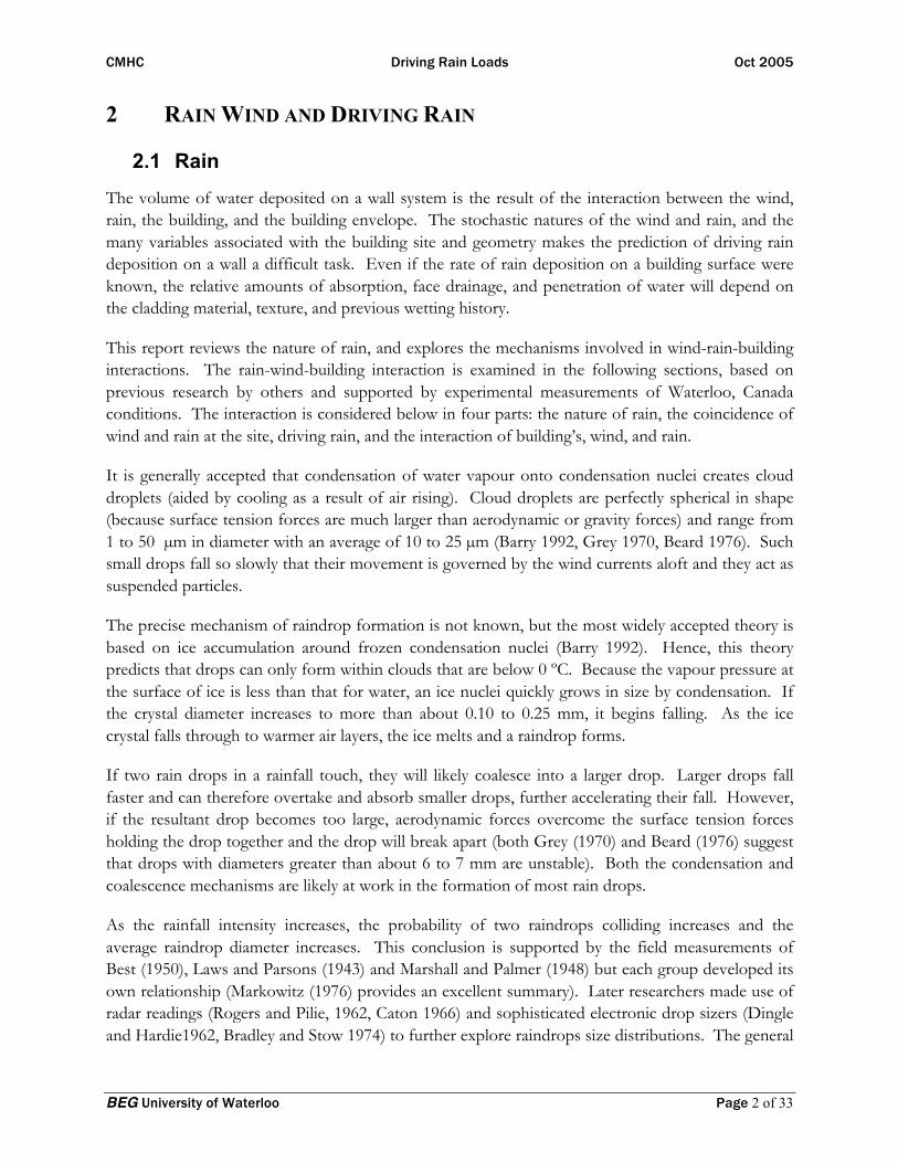
1 INTRODUCTION The University of Waterloo was awarded a grant under the Canada Mortgage and Housing Corporation’s External Research Program to develop driving rain loads on Canadian buildings. Using detailed hourly wind and rain data, driving rain is calculated.
This report summarizes the methods used, the type of data generated, and presents summarized results for use by building designers. A practical design method, partially validated with field data is presented for use.
1.1 The Importance of Driving Rain Loads The amount of water deposited on the above-grade building envelope by driving rain is larger than any other source of moisture in almost all building types and climates. Both the deposited rain absorbed by the cladding and water penetration of the cladding can be a significant source of moisture for many deterioration mechanisms. Despite the importance of driving rain to building performance, relatively little is known about the magnitude, duration, and frequency of driving rain and driving rain deposition on buildings.
Information about the magnitude and nature of the moisture load imposed by driving rain would be very useful and of practical value to many groups, such as:
• builders and designers of high-rise buildings, by assisting in the selection process for materials and systems, and assessing climate, orientation, height, and other performance related considerations
• manufacturers of bricks, siding, cladding and windows. The real knowledge of driving rain and its control should be of great value to designers and manufacturers of cladding systems, especially for export to markets in the United States, Asia, and Europe
• the restoration and repair industry, including product manufacturers, which will be able to make better decisions pertaining to renovation and repair of the huge stock of high-rise residential buildings,
• researchers and building science practitioners who require an in-depth understanding of driving rain in the natural environment as inputs for computer models so that they can predict wall behavior with more accuracy and confidence.
Codes and standards also may benefit from an improved knowledge of driving rain. Both new and prototype cladding and window systems are increasingly being tested for the control of driving rain before they are mass produced and installed. The standards used to define the test protocols were developed at least 30 years ago and embody the understanding of that time. Even with the current understanding of driving rain, it is clear that these standard test methods are not always appropriate for assessing the driving rain control provided by most modern cladding assemblies.
CMHC Driving Rain Loads Oct 2005
BEG University of Waterloo Page 2 of 33
2 RAIN WIND AND DRIVING RAIN
2.1 Rain The volume of water deposited on a wall system is the result of the interaction between the wind, rain, the building, and the building envelope. The stochastic natures of the wind and rain, and the many variables associated with the building site and geometry makes the prediction of driving rain deposition on a wall a difficult task. Even if the rate of rain deposition on a building surface were known, the relative amounts of absorption, face drainage, and penetration of water will depend on the cladding material, texture, and previous wetting history.
This report reviews the nature of rain, and explores the mechanisms involved in wind-rain-building interactions. The rain-wind-building interaction is examined in the following sections, based on previous research by others and supported by experimental measurements of Waterloo, Canada conditions. The interaction is considered below in four parts: the nature of rain, the coincidence of wind and rain at the site, driving rain, and the interaction of building’s, wind, and rain.
It is generally accepted that condensation of water vapour onto condensation nuclei creates cloud droplets (aided by cooling as a result of air rising). Cloud droplets are perfectly spherical in shape (because surface tension forces are much larger than aerodynamic or gravity forces) and range from 1 to 50 µm in diameter with an average of 10 to 25 µm (Barry 1992, Grey 1970, Beard 1976). Such small drops fall so slowly that their movement is governed by the wind currents aloft and they act as suspended particles.
The precise mechanism of raindrop formation is not known, but the most widely accepted theory is based on ice accumulation around frozen condensation nuclei (Barry 1992). Hence, this theory predicts that drops can only form within clouds that are below 0 ºC. Because the vapour pressure at the surface of ice is less than that for water, an ice nuclei quickly grows in size by condensation. If the crystal diameter increases to more than about 0.10 to 0.25 mm, it begins falling. As the ice crystal falls through to warmer air layers, the ice melts and a raindrop forms.
If two rain drops in a rainfall touch, they will likely coalesce into a larger drop. Larger drops fall faster and can therefore overtake and absorb smaller drops, further accelerating their fall. However, if the resultant drop becomes too large, aerodynamic forces overcome the surface tension forces holding the drop together and the drop will break apart (both Grey (1970) and Beard (1976) suggest that drops with diameters greater than about 6 to 7 mm are unstable). Both the condensation and coalescence mechanisms are likely at work in the formation of most rain drops.
As the rainfall intensity increases, the probability of two raindrops colliding increases and the average raindrop diameter increases. This conclusion is supported by the field measurements of Best (1950), Laws and Parsons (1943) and Marshall and Palmer (1948) but each group developed its own relationship (Markowitz (1976) provides an excellent summary). Later researchers made use of radar readings (Rogers and Pilie, 1962, Caton 1966) and sophisticated electronic drop sizers (Dingle and Hardie1962, Bradley and Stow 1974) to further explore raindrops size distributions. The general
CMHC Driving Rain Loads Oct 2005
BEG University of Waterloo Page 3 of 33
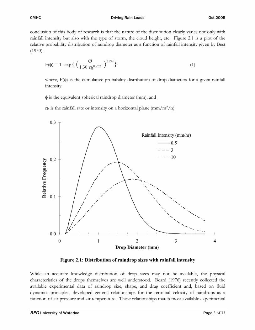
conclusion of this body of research is that the nature of the distribution clearly varies not only with rainfall intensity but also with the type of storm, the cloud height, etc. Figure 2.1 is a plot of the relative probability distribution of raindrop diameter as a function of rainfall intensity given by Best (1950):
F(φ) = 1- exp{-( Ø 1.30·rh0.232 )
2.245} (1)
where, F(φ) is the cumulative probability distribution of drop diameters for a given rainfall intensity
φ is the equivalent spherical raindrop diameter (mm), and
rh is the rainfall rate or intensity on a horizontal plane (mm/m2/h).
0.0
0.1
0.2
0.3
0 1 2 3 4Drop Diameter (mm)
Rel
ativ
e Fr
eque
ncy
0.5310
Rainfall Intensity (mm/hr)
Figure 2.1: Distribution of raindrop sizes with rainfall intensity
While an accurate knowledge distribution of drop sizes may not be available, the physical characteristics of the drops themselves are well understood. Beard (1976) recently collected the available experimental data of raindrop size, shape, and drag coefficient and, based on fluid dynamics principles, developed general relationships for the terminal velocity of raindrops as a function of air pressure and air temperature. These relationships match most available experimental
CMHC Driving Rain Loads Oct 2005
BEG University of Waterloo Page 4 of 33
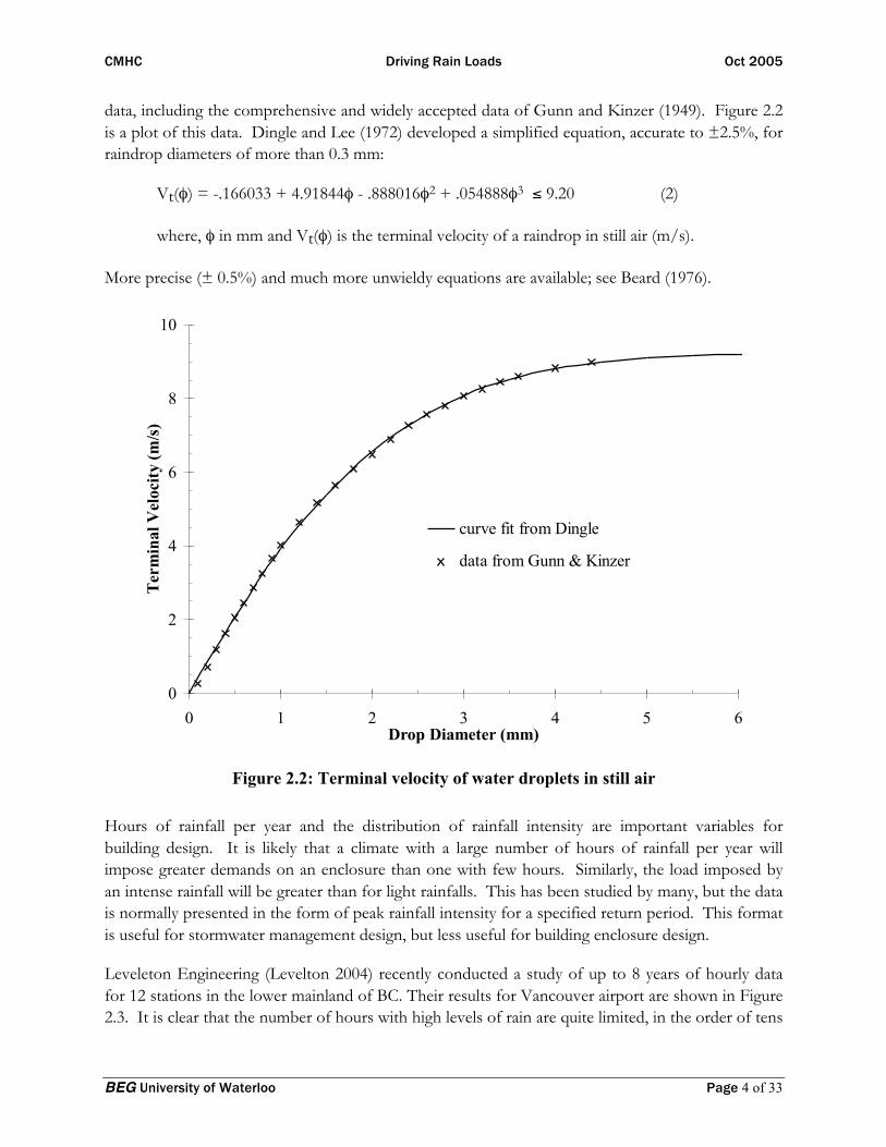
data, including the comprehensive and widely accepted data of Gunn and Kinzer (1949). Figure 2.2 is a plot of this data. Dingle and Lee (1972) developed a simplified equation, accurate to ±2.5%, for raindrop diameters of more than 0.3 mm:
Vt(φ) = -.166033 + 4.91844φ - .888016φ2 + .054888φ3 ≤ 9.20 (2)
where, φ in mm and Vt(φ) is the terminal velocity of a raindrop in still air (m/s).
More precise (± 0.5%) and much more unwieldy equations are available; see Beard (1976).
0
2
4
6
8
10
0 1 2 3 4 5 6Drop Diameter (mm)
Term
inal
Vel
ocity
(m/s)
curve fit from Dingle
data from Gunn & Kinzer
Figure 2.2: Terminal velocity of water droplets in still air
Hours of rainfall per year and the distribution of rainfall intensity are important variables for building design. It is likely that a climate with a large number of hours of rainfall per year will impose greater demands on an enclosure than one with few hours. Similarly, the load imposed by an intense rainfall will be greater than for light rainfalls. This has been studied by many, but the data is normally presented in the form of peak rainfall intensity for a specified return period. This format is useful for stormwater management design, but less useful for building enclosure design.
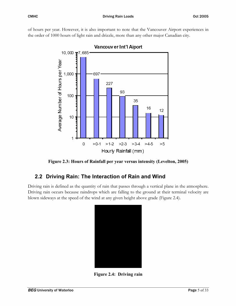
Leveleton Engineering (Levelton 2004) recently conducted a study of up to 8 years of hourly data for 12 stations in the lower mainland of BC. Their results for Vancouver airport are shown in Figure 2.3. It is clear that the number of hours with high levels of rain are quite limited, in the order of tens
CMHC Driving Rain Loads Oct 2005
BEG University of Waterloo Page 5 of 33
of hours per year. However, it is also important to note that the Vancouver Airport experiences in the order of 1000 hours of light rain and drizzle, more than any other major Canadian city.
Figure 2.3: Hours of Rainfall per year versus intensity (Levelton, 2005)
2.2 Driving Rain: The Interaction of Rain and Wind Driving rain is defined as the quantity of rain that passes through a vertical plane in the atmosphere. Driving rain occurs because raindrops which are falling to the ground at their terminal velocity are blown sideways at the speed of the wind at any given height above grade (Figure 2.4).
Figure 2.4: Driving rain
CMHC Driving Rain Loads Oct 2005
BEG University of Waterloo Page 6 of 33
The amount of driving rain in unobstructed wind flow can be calculated with reasonable accuracy. The speed at which raindrops fall is a function of the size of the drop. Essentially, as the drop size increases the rain drop terminal speed increases at a decreasing rate. The wind carries the drops along horizontally due to drag. The combination of gravity and wind forces determines the trajectory of the drop, and simple geometry can then be used to assess the amount of rain passing through a vertical plane. Complicating this assessment is the fact that there is a range of raindrop sizes in any rainstorm. Research by various meteorologists can be used to correlate the distribution of drop sizes in a rainstorm with the intensity of the rainfall.
Based on this type of approach Lacy [1965] proposed a simple equation relating wind speed and rainfall intensity to driving rain:
rv = 0.208 · V· rh (3)
where, rv is the rate of rain passing through a vertical plane (l/m2/h),
V is the average wind velocity (m/s), and
rh is the average rainfall rate on a horizontal plane such as the ground (mm/m2/h).
This equation was based on a mix of his field measurements and some theoretical considerations. Subsequent theoretical work and a considerable amount of field measurement [Straube 1998] has allowed us to extend and generalize Equation 3 to
rv = DRF · V(z) · rh (4)
where V(z) is the wind speed at, z, the height of interest (m/s),
The proportionality constant in Equation (4), is the ratio of rain on a vertical plane (driving rain) to rain on a horizontal plane (falling rain) and has been defined [Straube & Burnett 1997] as the driving rain factor (DRF). From simple geometry, it can be seen that the Driving Rain Factor is equal to the inverse of the terminal drop velocity:
DRF =1/Vt (5)
Field studies at the University of Waterloo [Straube & Burnett 1997], in Germany [Kuenzel 1994] and computer models [Choi 1994] have found that the value for the DRF ranges between 0.20 to 0.25 for average conditions. This is the reason that the simple semi-empirical Lacy equation was so successful. However, DRF does vary considerably for different rainfall intensities and rain storm types. For example, it can range from more than 0.5 for drizzle to as little as 0.15 for intense cloudbursts.
The cosine of the angle between the plane of interest and the direction of the wind can be used to account for wind direction on a plane oriented in a specific direction.
rv = DRF · V(z) · rh· cos θ (6)
CMHC Driving Rain Loads Oct 2005
BEG University of Waterloo Page 7 of 33
where θ is the angle between a line drawn perpendicular to the wall of interest and the wind direction.
Experimental work [Straube 1998] has shown that the quantity of driving rain in an unobstructed wind flow can be calculated with an accuracy of better than 10% using Equations 2, 5 and 6, provided the median raindrop diameter predicted by Equation 1 is used.
2.3 The Coincidence of Rain and Wind As shown, windspeed has a direct effect on the amount of driving rain It cannot, however, be assumed that the wind and falling rain can be modelled as statistically independent events. In fact, there is strong evidence to suggest that the wind-speed probability distribution is somewhat different during rain events. It is also well documented that the wind direction distribution is different during rain events (e.g., Skerlj 1999). Although all climates are not the same, the Surry study (Surry et al 1995) did find many climates in which the predominant wind direction was quite different than the wind direction during rain (for example, see Figure 2.5).
The importance of wind speed to the intensity of driving rain can be calculated using the methods outlined above. However, high wind speeds also may generate high stagnation pressures that can drive rain into the cracks and openings of some types of enclosures. Wind speed can be converted to a stagnation air pressure (assuming a temperature of 15° C) using Equation 7.
Pstag = 0.6 · V2 (7)
Where V is the windspeed [m/s] and
Pstag is the stagnation pressure [Pa]
Small flaws in non-absorptive face-sealed claddings for example, may leak significantly more when exposed to pressure differences [Lacasse et al 2003]. However, brickwork does not leak significantly more under pressures of 50 Pa than 0 Pa [Straube and Burnett 2000]. In most cases the increase in air pressure is less important than the increase in water deposition, and lab testing provides some support for this contention [Lacasse et al 2003]. Hence, although practitioners often observe an increase in rain-penetration control problems in high exposure conditions much of the evidence suggests that these problems are usually due not to an increase in air pressure difference but to an increase in rain deposition.
CMHC Driving Rain Loads Oct 2005
BEG University of Waterloo Page 8 of 33
Figure 2.5: Wind Direction during Rain and During all hours for St John’s NFLD [Surry et al 1995]
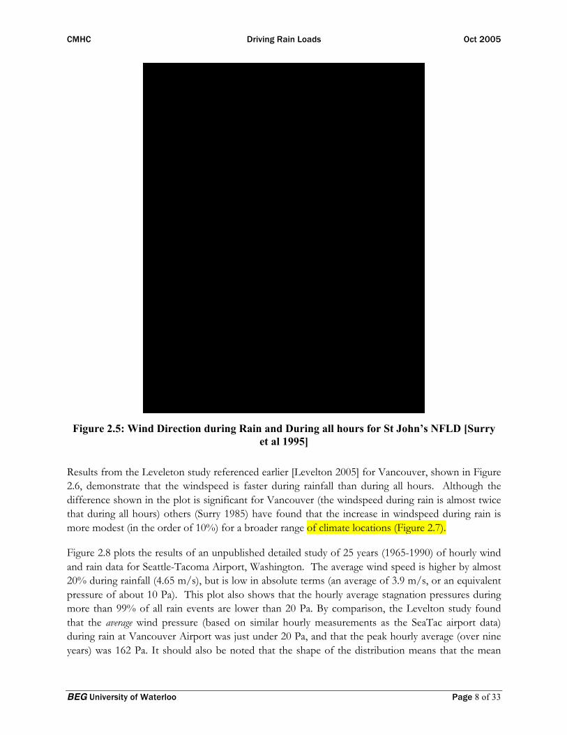
Results from the Leveleton study referenced earlier [Levelton 2005] for Vancouver, shown in Figure 2.6, demonstrate that the windspeed is faster during rainfall than during all hours. Although the difference shown in the plot is significant for Vancouver (the windspeed during rain is almost twice that during all hours) others (Surry 1985) have found that the increase in windspeed during rain is more modest (in the order of 10%) for a broader range of climate locations (Figure 2.7).
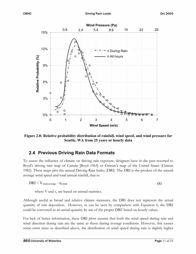
Figure 2.8 plots the results of an unpublished detailed study of 25 years (1965-1990) of hourly wind and rain data for Seattle-Tacoma Airport, Washington. The average wind speed is higher by almost 20% during rainfall (4.65 m/s), but is low in absolute terms (an average of 3.9 m/s, or an equivalent pressure of about 10 Pa). This plot also shows that the hourly average stagnation pressures during more than 99% of all rain events are lower than 20 Pa. By comparison, the Levelton study found that the average wind pressure (based on similar hourly measurements as the SeaTac airport data) during rain at Vancouver Airport was just under 20 Pa, and that the peak hourly average (over nine years) was 162 Pa. It should also be noted that the shape of the distribution means that the mean
CMHC Driving Rain Loads Oct 2005
BEG University of Waterloo Page 9 of 33
(average) and median (the value which is more than half of all samples) windspeed are quite different – a few hours per year experience high speeds, and this increases the average.
Figure 2.6: Rainfall Intensity versus Windspeed for Vancouver (Levelton 2004) Light bars are during rain. Dark bars are all hours
CMHC Driving Rain Loads Oct 2005
BEG University of Waterloo Page 10 of 33
Figure 2.7: Rainfall Hours for various Canadian locations (Surry 1995)
CMHC Driving Rain Loads Oct 2005
BEG University of Waterloo Page 11 of 33
0%
3%
6%
9%
12%
15%
0 1 2 3 4 5 6 7
Wind Speed (m/s)
Rel
ativ
e Pr
obab
ility
(%)
During RainAll hours
Wind Pressure (Pa)2.4 5.4 9.6 15 22 290.6
Figure 2.8: Relative probability distribution of rainfall, wind speed, and wind pressure for Seattle, WA from 25 years or hourly data
2.4 Previous Driving Rain Data Formats To assess the influence of climate on driving rain exposure, designers have in the past resorted to Boyd's driving rain map of Canada [Boyd 1963] or Grimm’s map of the United States (Grimm 1982). These maps plot the annual Driving Rain Index (DRI). The DRI is the product of the annual average wind speed and total annual rainfall, that is:
DRI = Vwind,average · rh,total (8)
where V and rh are based on annual statistics.
Although useful as broad and relative climate measures, the DRI does not represent the actual quantity of rain deposition. However, as can be seen by comparison with Equation 6, the DRI could be converted to an actual quantity by use of the proper DRF based on hourly values.
For lack of better information, these DRI plots assume that both the wind speed during rain and wind direction during rain are the same as those during average conditions. However, this causes some error since as described above, the distribution of wind speed during rain is slightly higher
CMHC Driving Rain Loads Oct 2005
BEG University of Waterloo Page 12 of 33
(typically 10 to 20% higher) than during all hours and the wind direction during rainfall is often quite different than during non-rainy hours [Surrey et al 1995, Skerlj 1999]. Both of these conclusions are climate dependent.
A further limitation of the application of DRI plots to building design is that they do not reflect the impact of orientation and exposure. It is clear to practitioners that different localities have different building faces with significantly higher rain deposition and that a bungalow is exposed differently than a high rise building on a hilltop.
It is this need for more accurate plots of driving rain that reflect the different climates of Canada, account for the actual distribution of wind speed and rain fall intensity, and account for wind direction during rain, that prompted this research project.
2.5 Previous Driving Rain Research
2.5.1 Field Measurements
Driving rain has been investigated by building scientists and meteorologists in the field for many years. Driving rain has been measured under real conditions in Europe for at least 75 years (continuously for more than 50 years at one location we know of) although not usually on building systems. Lacy conducted the seminal English language study in the early 1960’s, but his study was mostly aimed at driving rain in the free wind and during average rain events (Lacy 1965). Boyd (1963) generated a Canadian driving rain map in 1963 based mostly on Lacy’s work, but this dealt only with driving rain in open fields away from buildings. Baker and Robinson of IRC/NRCC produced an excellent and still valid qualitative study of driving rain wetting patterns and staining.
Driving rain has been measured on an increasing number of buildings. Early studies (in the early 90’s) were focused at IRC/NRCC, who mounted several gauges on a three story building. An array of 15 driving rain gauges were installed on a test hut at the University of Waterloo in 1994, with the express intent of improving our understanding of the distribution of rain. As part of the MEWS study, this author installed arrays of gauges on a 4 storey apartment in Kitchener and a large high-bay industrial building in Vancouver in 1999. Five of the same UW gauges were installed by RDH Building Engineering on building retrofits in Vancouver as part of another research project (funded by CMHC, the Homeowner Protection Office and the BC Housing Management Commission). Finally, higher resolution commercial driving rain gauges have been installed on numerous test buildings around North America (North Carolina, Georgia, Washington, Minnesota, Alaska). All of this research, supported by results from the UW testhut facility and MEWS monitoring, suggest that driving rain can be rationally predicted (Straube 1997, 1998).
2.5.2 Modeling
Initial research, in Singapore by Choi (1993), and at IRC/NRCC by Karagiozis and Hadjisophocieous (1995, 1997), has attempted to develop predictive computer models of rain wetting with mixed results. Work by others, such as Wisse (1994), and Van Mook (1999)
CMHC Driving Rain Loads Oct 2005
BEG University of Waterloo Page 13 of 33
developed the modelling of driving rain further. Both wind tunnel and computer models however, require validation and calibration with real data. Recent work in Europe (Blocken and Carmeliet 2000) has provided some comparison between field studies and models and hence more confidence that computer models may provide useful data. CMHC also provided support to study driving rain in the Boundary Layer Wind Tunnel at the University of Western Ontario (Inculet and Surry 1995). This provided indications as to the distribution of rain deposition on tall buildings and the impact of overhangs.
2.6 Testing and Standards related to Driving Rain One of the uses of driving rain data is to develop and interpret building enclosure component or assembly test results. A brief review of the rain deposition rates and standard tests is therefore useful.
The ASTM Standard E331 "Standard Test Method for Water Penetration of Exterior Windows, Curtain Walls, and Doors by Uniform Static Air Pressure Difference" is widely used. This standard employs a uniform static air pressure difference of at least 137 Pa (equivalent to a windspeed of about 15 m/s or over 50 km/h) during the application of a water spray with a minimum rate of 203 mm/hr. The test lasts 15 minutes and any points of water leakage are recorded and described. For masonry walls, ASTM Standard E514 “Standard Test Method for Water Penetration and Leakage Through Masonry” is used. This method imposes loads of 138 l/m2/hr and a pressure of 500 Pa (equal to a wind speed 28 m/s or 100 km/h) for at least 4 hours.
The CSA A-440 Window standard incorporates Driving Rain Wind Pressures (DRWP) as a method of selecting windows to resist driving rain. These pressures were developed by Welsh, Skinner, and Morris (1989) using an hourly rainfall threshold of 1.8 mm/h and five and ten year return periods. Although no driving rain intensities were predicted, air pressures for many Canadian locations were provided. These pressures are the highest hourly average pressures that would be experienced in 5 or in 10 years. The worst hour may be of interest to an enclosure component such as a window, which has no moisture storage capacity. Even so, a leak every 5 to 10 years may not be a problem, since the typically small amount of leakage would quickly evaporate. It is more likely that repeated leaks, many per year, over several years, will result in more serious enclosure deterioration than a single leak of somewhat larger magnitude. Hence, information regarding more common wind pressures and driving rain would be useful.
In brief, test standards apply rates of water of about 100 to 200 l/m2/hr, at pressures equivalent to a stagnation pressure generated by a windspeed of 15 to 28 m/s. These test values can be compared to the results generated later in this report.
3 DRIVING RAIN DATA Hourly weather files were purchased from the Meteorological Service of Canada, Environment Canada. Of the thousands of monitoring locations, we selected those that provided:
CMHC Driving Rain Loads Oct 2005
BEG University of Waterloo Page 14 of 33
1. hourly observations
2. more than ten years of data (to provide a reasonable basis for annual average statistics)
3. wind speed, wind direction, and rainfall weather elements
4. data collection after 1965 (since this is when the anemometers of many stations were moved to provide consistent open wind measurements without the sheltering effect of obstructions), and
5. a range of major population centres and a broad geographic distribution.
These restrictions reduced the available number of stations to less than 100, well distributed across Canada. However, it was found that there is no set of data available that combine hourly rain and wind. Hence, it was necessary to combine the CWEEDS (Canadian Weather Energy and Engineering Data Sets) files (which contain wind speed and direction) and the Environment Canada HLY03 data set (which contain hourly rainfall data).
In some cases the hourly rainfall data was not available but an hourly weather flag (which indicates weather conditions, not quantitative rainfall) was. In many cases, data beyond 1989 was not available. To account for hours in which no rain was reported (in the HLY03 files) but hourly observations were (in the CWEEDS files), the Atmospheric Environment Service (AES 1984) equivalent rain rates were used: 1.8 mm/hr for light, 5.1 for moderate and 13.0 for heavy rain.
Driving rain data were calculated using equations 1, 2, and 5 and the hourly weather data files created. Each of the cities data from 1965 to 1989 (25 years) was stored in a data file which occupied approximately 9 MB.
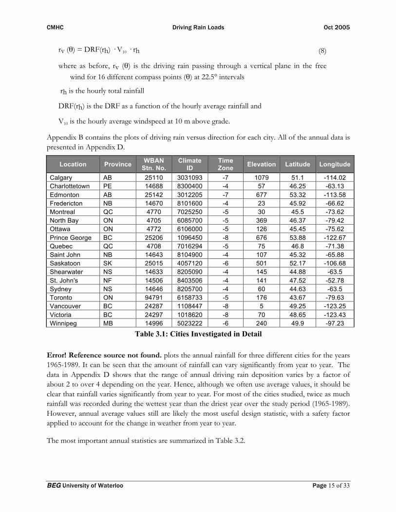
Eighteen major Canadian cities were investigated in detail. These are listed and described in the Table 3.1.
The data calculated for each year 1965-1989 included:
1. Annual rainfall and number of hours of rainfall
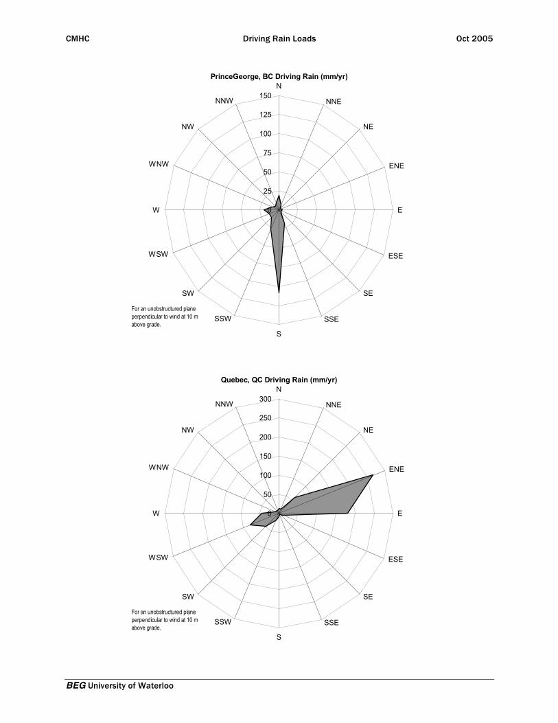
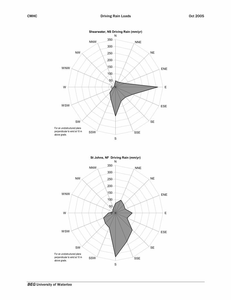
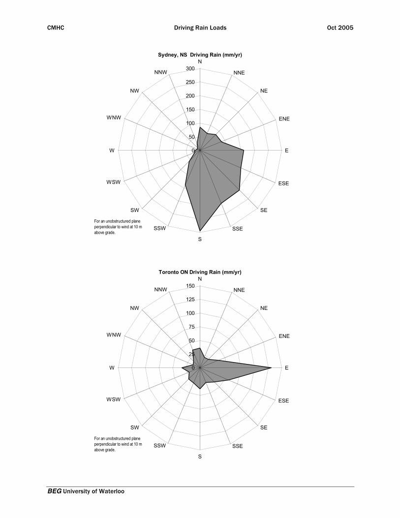
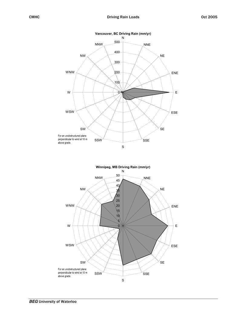
2. Annual driving rain from each direction of a 16 point compass
3. Total Annual Driving Rain
4. Annual driving rain on a wall facing each direction of a 16 point compass
5. Peak annual driving Rain and Direction
6. Windspeed vs direction during all hours and during rainy hours
Driving rain data was calculated from the data files using
CMHC Driving Rain Loads Oct 2005
BEG University of Waterloo Page 15 of 33
rv (θ) = DRF(rh) · V10 · rh (8)
where as before, rv (θ) is the driving rain passing through a vertical plane in the free wind for 16 different compass points (θ) at 22.5° intervals
rh is the hourly total rainfall
DRF(rh) is the DRF as a function of the hourly average rainfall and
V10 is the hourly average windspeed at 10 m above grade.
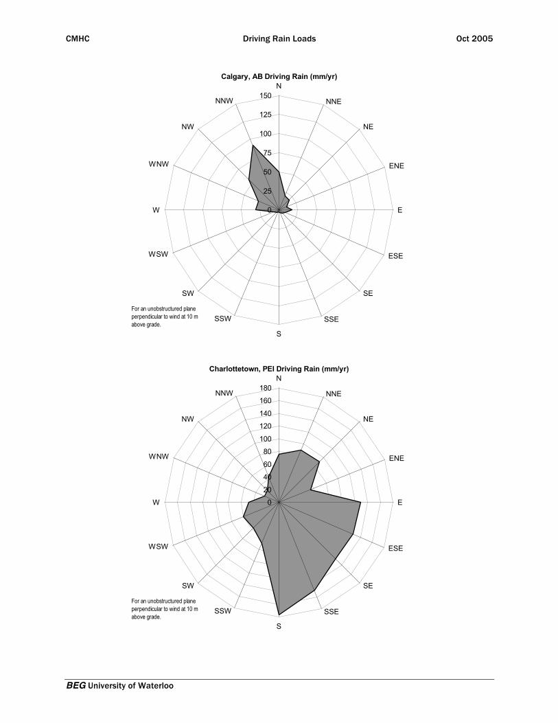
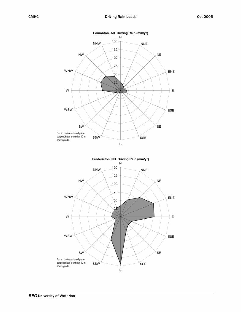
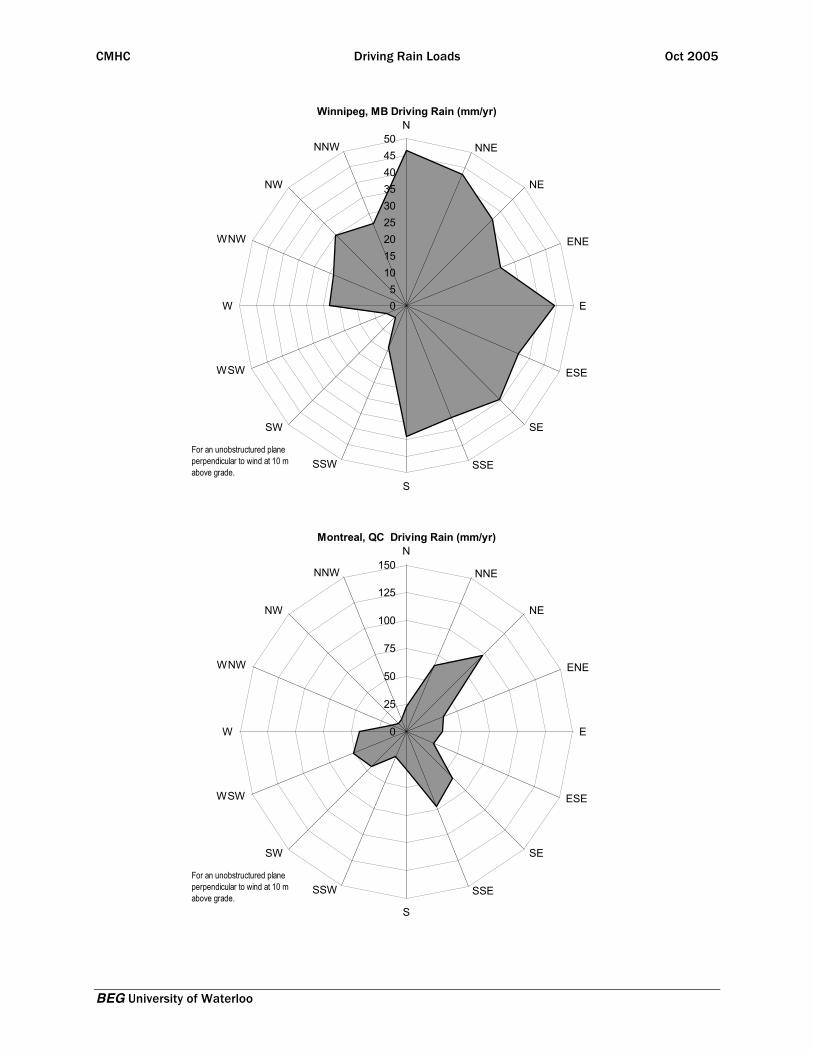
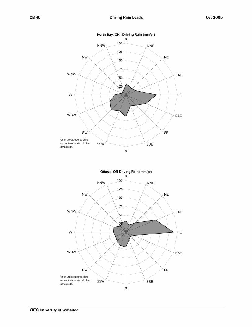
Appendix B contains the plots of driving rain versus direction for each city. All of the annual data is presented in Appendix D.
Location Province WBAN Stn. No.
Climate ID
Time Zone Elevation Latitude Longitude
Calgary AB 25110 3031093 -7 1079 51.1 -114.02 Charlottetown PE 14688 8300400 -4 57 46.25 -63.13 Edmonton AB 25142 3012205 -7 677 53.32 -113.58 Fredericton NB 14670 8101600 -4 23 45.92 -66.62 Montreal QC 4770 7025250 -5 30 45.5 -73.62 North Bay ON 4705 6085700 -5 369 46.37 -79.42 Ottawa ON 4772 6106000 -5 126 45.45 -75.62 Prince George BC 25206 1096450 -8 676 53.88 -122.67 Quebec QC 4708 7016294 -5 75 46.8 -71.38 Saint John NB 14643 8104900 -4 107 45.32 -65.88 Saskatoon SK 25015 4057120 -6 501 52.17 -106.68 Shearwater NS 14633 8205090 -4 145 44.88 -63.5 St. John's NF 14506 8403506 -4 141 47.52 -52.78 Sydney NS 14646 8205700 -4 60 44.63 -63.5 Toronto ON 94791 6158733 -5 176 43.67 -79.63 Vancouver BC 24287 1108447 -8 5 49.25 -123.25 Victoria BC 24297 1018620 -8 70 48.65 -123.43 Winnipeg MB 14996 5023222 -6 240 49.9 -97.23
Table 3.1: Cities Investigated in Detail
Error! Reference source not found. plots the annual rainfall for three different cities for the years 1965-1989. It can be seen that the amount of rainfall can vary significantly from year to year. The data in Appendix D shows that the range of annual driving rain deposition varies by a factor of about 2 to over 4 depending on the year. Hence, although we often use average values, it should be clear that rainfall varies significantly from year to year. For most of the cities studied, twice as much rainfall was recorded during the wettest year than the driest year over the study period (1965-1989). However, annual average values still are likely the most useful design statistic, with a safety factor applied to account for the change in weather from year to year.
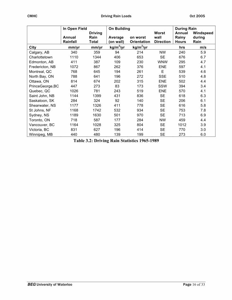
The most important annual statistics are summarized in Table 3.2.
CMHC Driving Rain Loads Oct 2005
BEG University of Waterloo Page 16 of 33
In Open Field On Building During Rain
Annual Rainfall
Driving Rain Total
Average (on wall)
on worst Orientation
Worst wall Direction
Annual Rainy Hours
Windspeed during Rain
City mm/yr mm/yr kg/m2/yr kg/m2/yr hrs m/s Calgary, AB 340 359 94 214 NW 240 5.9 Charlottetown 1110 1344 406 653 SE 676 6.7 Edmonton, AB 411 387 109 230 WNW 295 4.7 Fredericton, NB 1072 867 262 376 ENE 597 4.1 Montreal, QC 768 645 194 261 E 539 4.6 North Bay, ON 788 641 196 272 SSE 510 4.8 Ottawa, ON 814 674 202 315 ENE 502 4.4 PrinceGeorge,BC 447 273 83 173 SSW 394 3.4 Quebec, QC 1026 781 243 519 ENE 570 4.1 Saint John, NB 1144 1399 431 836 SE 618 6.3 Saskatoon, SK 284 324 92 140 SE 206 6.1 Shearwater, NS 1177 1326 411 778 SE 616 5.8 St Johns, NF 1168 1742 532 934 SE 753 7.8 Sydney, NS 1189 1630 501 970 SE 713 6.9 Toronto, ON 718 587 177 284 NW 459 4.4 Vancouver, BC 1164 1028 325 804 SE 1012 3.9 Victoria, BC 831 627 196 414 SE 770 3.0 Winnipeg, MB 440 480 139 199 SE 273 6.0
Table 3.2: Driving Rain Statistics 1965-1989

CMHC Driving Rain Loads Oct 2005
BEG University of Waterloo Page 17 of 33
0
200
400
600
800
1000
1200
1400
1600
1965
1967
1969
1971
1973
1975
1977
1979
1981
1983
1985
1987
1989
Ann
ual R
ainf
all [
mm
]Edmonton
Toronto
Vancouver
Figure 3.1: Annual Rainfall versus year for selected Cities
CMHC Driving Rain Loads Oct 2005
BEG University of Waterloo Page 18 of 33
0
100
200
300
400
500
600
700
800
900
1000
1100
Saska
toon
Calgary
Winnipe
g
Edmon
ton
Prince
Geo
rge
Toronto
North B
ay
Ottawa
Montre
al
Quebe
c
Shearw
ater
Saint J
ohn
Frederi
cton
Charlo
ttetow
n
Sydne
y
St Joh
ns
Victori
a
Vanco
uver
Ann
ual A
vera
ge R
ainy
Hou
rs (b
ased
on
1965
-198
9)
.
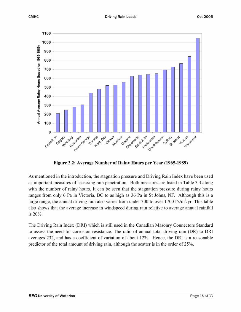
Figure 3.2: Average Number of Rainy Hours per Year (1965-1989)
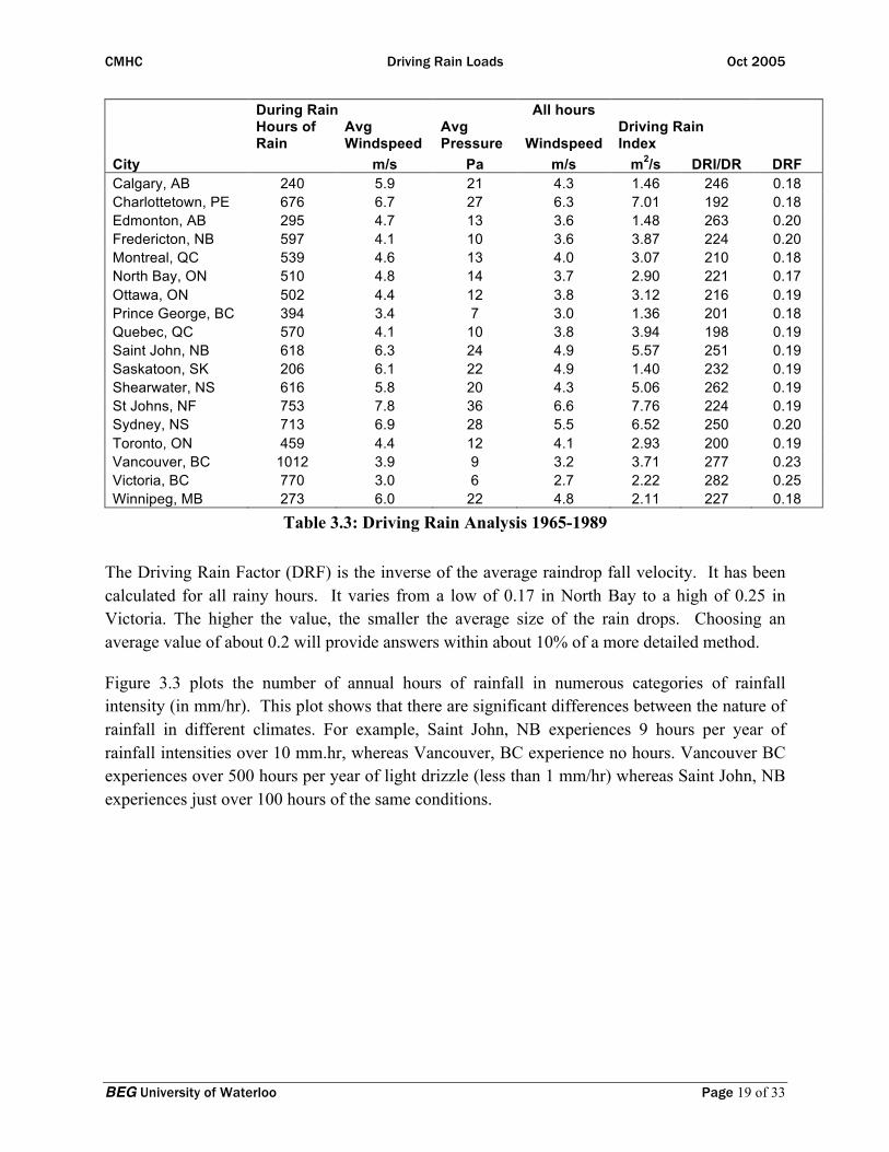
As mentioned in the introduction, the stagnation pressure and Driving Rain Index have been used as important measures of assessing rain penetration. Both measures are listed in Table 3.3 along with the number of rainy hours. It can be seen that the stagnation pressure during rainy hours ranges from only 6 Pa in Victoria, BC to as high as 36 Pa in St Johns, NF. Although this is a large range, the annual driving rain also varies from under 300 to over 1700 l/s/m2/yr. This table also shows that the average increase in windspeed during rain relative to average annual rainfall is 20%.
The Driving Rain Index (DRI) which is still used in the Canadian Masonry Connectors Standard to assess the need for corrosion resistance. The ratio of annual total driving rain (DR) to DRI averages 232, and has a coefficient of variation of about 12%. Hence, the DRI is a reasonable predictor of the total amount of driving rain, although the scatter is in the order of 25%.
CMHC Driving Rain Loads Oct 2005
BEG University of Waterloo Page 19 of 33
During Rain All hours
Hours of Rain
Avg Windspeed
Avg Pressure Windspeed
Driving Rain Index
City m/s Pa m/s m2/s DRI/DR DRF Calgary, AB 240 5.9 21 4.3 1.46 246 0.18 Charlottetown, PE 676 6.7 27 6.3 7.01 192 0.18 Edmonton, AB 295 4.7 13 3.6 1.48 263 0.20 Fredericton, NB 597 4.1 10 3.6 3.87 224 0.20 Montreal, QC 539 4.6 13 4.0 3.07 210 0.18 North Bay, ON 510 4.8 14 3.7 2.90 221 0.17 Ottawa, ON 502 4.4 12 3.8 3.12 216 0.19 Prince George, BC 394 3.4 7 3.0 1.36 201 0.18 Quebec, QC 570 4.1 10 3.8 3.94 198 0.19 Saint John, NB 618 6.3 24 4.9 5.57 251 0.19 Saskatoon, SK 206 6.1 22 4.9 1.40 232 0.19 Shearwater, NS 616 5.8 20 4.3 5.06 262 0.19 St Johns, NF 753 7.8 36 6.6 7.76 224 0.19 Sydney, NS 713 6.9 28 5.5 6.52 250 0.20 Toronto, ON 459 4.4 12 4.1 2.93 200 0.19 Vancouver, BC 1012 3.9 9 3.2 3.71 277 0.23 Victoria, BC 770 3.0 6 2.7 2.22 282 0.25 Winnipeg, MB 273 6.0 22 4.8 2.11 227 0.18
Table 3.3: Driving Rain Analysis 1965-1989
The Driving Rain Factor (DRF) is the inverse of the average raindrop fall velocity. It has been calculated for all rainy hours. It varies from a low of 0.17 in North Bay to a high of 0.25 in Victoria. The higher the value, the smaller the average size of the rain drops. Choosing an average value of about 0.2 will provide answers within about 10% of a more detailed method.
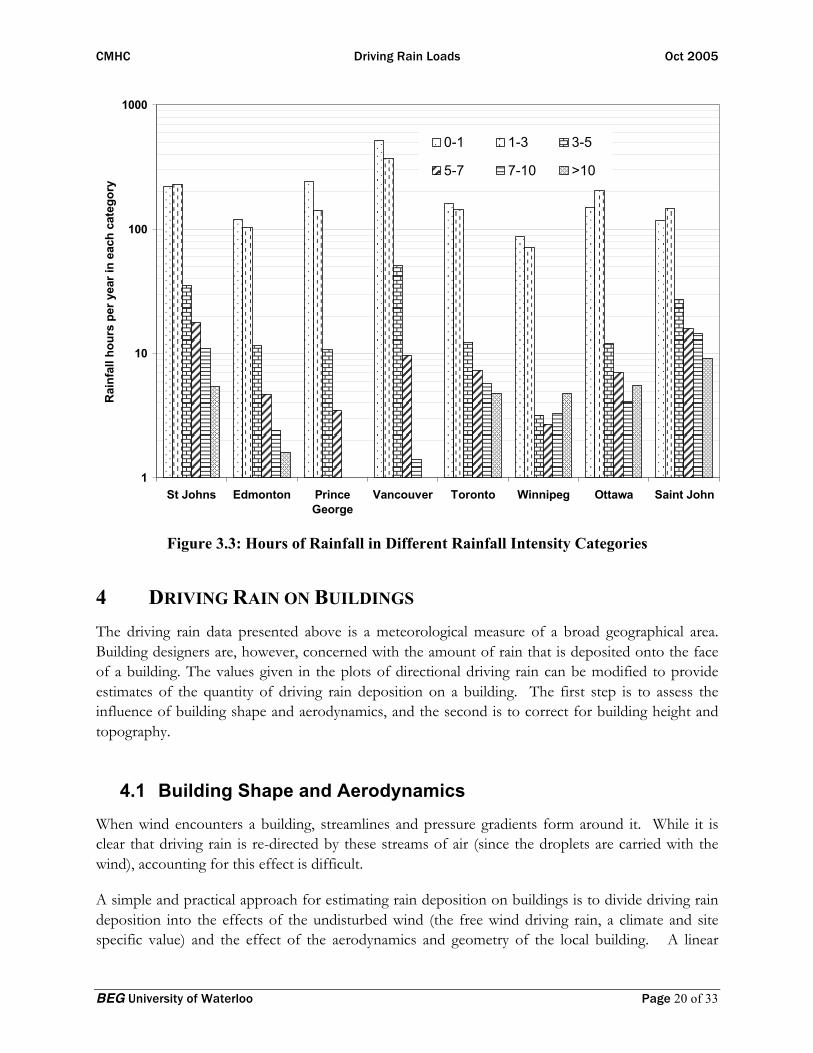
Figure 3.3 plots the number of annual hours of rainfall in numerous categories of rainfall intensity (in mm/hr). This plot shows that there are significant differences between the nature of rainfall in different climates. For example, Saint John, NB experiences 9 hours per year of rainfall intensities over 10 mm.hr, whereas Vancouver, BC experience no hours. Vancouver BC experiences over 500 hours per year of light drizzle (less than 1 mm/hr) whereas Saint John, NB experiences just over 100 hours of the same conditions.
CMHC Driving Rain Loads Oct 2005
BEG University of Waterloo Page 20 of 33
1
10
100
1000
St Johns Edmonton PrinceGeorge
Vancouver Toronto Winnipeg Ottawa Saint John
Rai
nfal
l hou
rs p
er y
ear i
n ea
ch c
ateg
ory
0-1 1-3 3-5
5-7 7-10 >10
Figure 3.3: Hours of Rainfall in Different Rainfall Intensity Categories
4 DRIVING RAIN ON BUILDINGS The driving rain data presented above is a meteorological measure of a broad geographical area. Building designers are, however, concerned with the amount of rain that is deposited onto the face of a building. The values given in the plots of directional driving rain can be modified to provide estimates of the quantity of driving rain deposition on a building. The first step is to assess the influence of building shape and aerodynamics, and the second is to correct for building height and topography.
4.1 Building Shape and Aerodynamics When wind encounters a building, streamlines and pressure gradients form around it. While it is clear that driving rain is re-directed by these streams of air (since the droplets are carried with the wind), accounting for this effect is difficult.
A simple and practical approach for estimating rain deposition on buildings is to divide driving rain deposition into the effects of the undisturbed wind (the free wind driving rain, a climate and site specific value) and the effect of the aerodynamics and geometry of the local building. A linear

CMHC Driving Rain Loads Oct 2005
BEG University of Waterloo Page 21 of 33
factor, the rain deposition factor (RDF), can be used to transforms the rate of driving rain in the free wind (i.e. outside of the region disturbed by a building) to the rate of rain deposition on a particular building (Straube 1998). Section 3 presented driving rain data for the free wind. For a particular orientation and spot on the building face, the free wind driving rain values can be modified as:
rvb = RDF · DRF · V(z) · cos (θ ) · rh (9)
where rvb is the rain deposition rate on a vertical building surface(l/m2/h),
RDF is the Rain Deposition Factor, the ratio of rain in the free wind to rain deposition on a building, which accounts for the effect of building shape and size on rain deposition.
DRF is the Driving Rain Factor, which accounts for interaction of the wind and rain in the undisturbed wind,
θ is the angle between the normal to the wall and the wind direction, and
V(z) is the windspeed in m/s at z meters above grade.
Driving rain data on a standard building face was calculated from the data files using:
rbv (θ) = DRF(rh) · RDF· V10 · rh · cos (θ ) for all +/-90°. (10)
where all variables are as before.
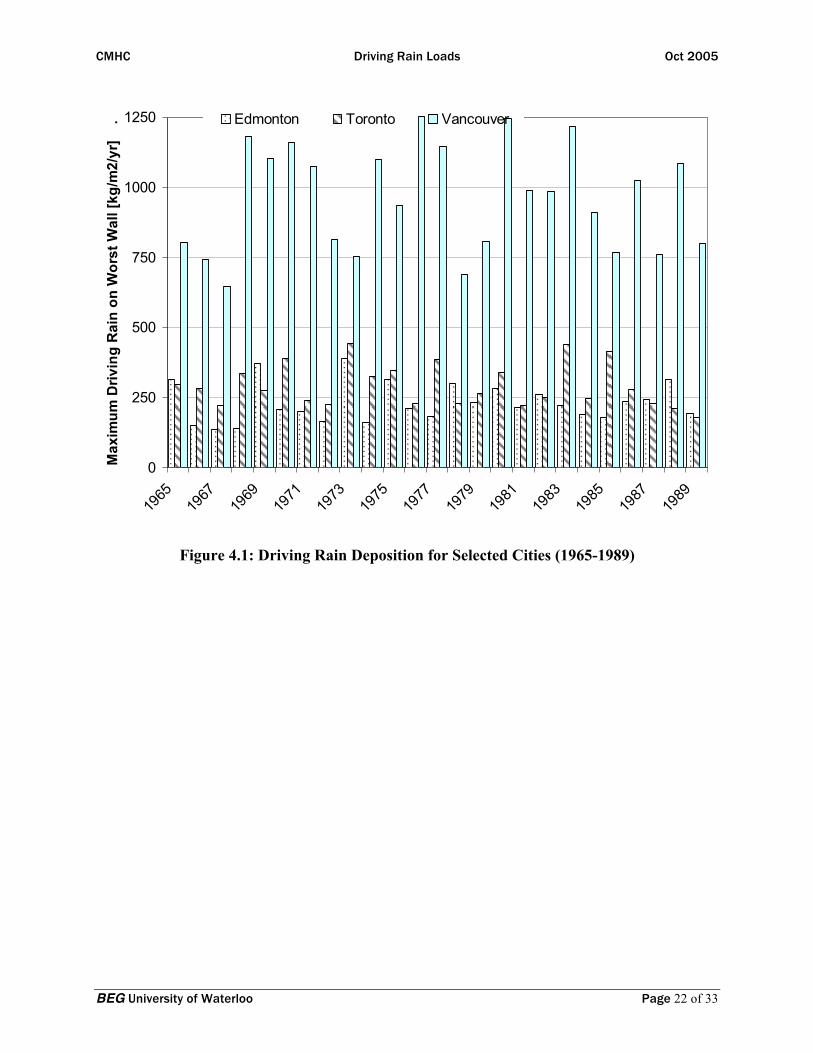
This equation was used to calculate the driving rain on a nominal building at 10 m above grade, in flat, open terrain, with an RDF =1. The data for 18 Canadian cities is presented in Appendix C and the numerical data for each year (1965-1989) is tabulated in Appendix D.
As expected, the variation in driving rain is similar year-to-year as rainfall.
CMHC Driving Rain Loads Oct 2005
BEG University of Waterloo Page 22 of 33
0
250
500
750
1000
1250
1965
1967
1969
1971
1973
1975
1977
1979
1981
1983
1985
1987
1989
Max
imum
Driv
ing
Rai
n on
Wor
st W
all [
kg/m
2/yr
] .
Edmonton Toronto Vancouver
Figure 4.1: Driving Rain Deposition for Selected Cities (1965-1989)
CMHC Driving Rain Loads Oct 2005
BEG University of Waterloo Page 23 of 33
0
200
400
600
800
1000
Calgary
, AB
Edmon
ton, A
B
Prince
Geo
rge, B
C
Vanco
uver,
BC
Victori
a, BC
Winnipe
g, MB
Frederi
cton,
NB
Saint J
ohn,
NB
St Joh
ns, N
F
Shearw
ater, N
S
Sydne
y, NS
North B
ay, O
N
Ottawa,
ON
Toronto
, ON
Charlo
ttetow
n, PE
Montre
al, Q
C
Quebe
c, QC
Saska
toon,
SK
Max
imum
Driv
ing
Rai
n on
Wor
st W
all [
kg/m
2 /yr]
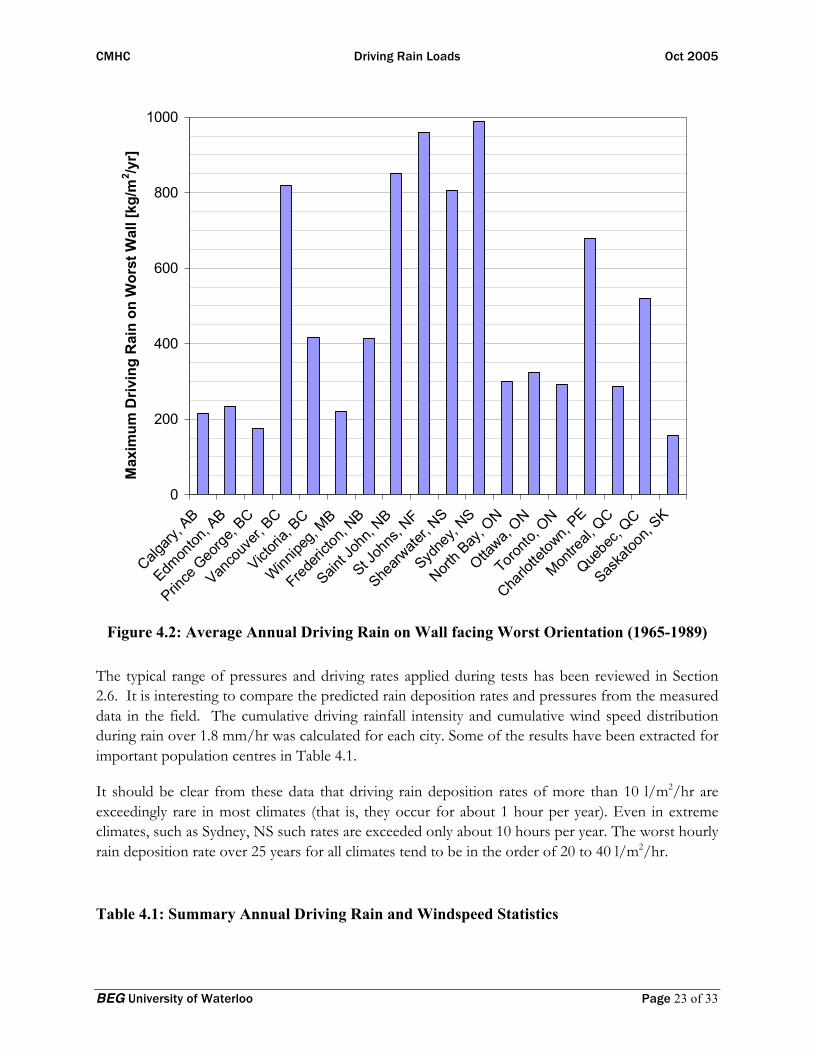
Figure 4.2: Average Annual Driving Rain on Wall facing Worst Orientation (1965-1989)
The typical range of pressures and driving rates applied during tests has been reviewed in Section 2.6. It is interesting to compare the predicted rain deposition rates and pressures from the measured data in the field. The cumulative driving rainfall intensity and cumulative wind speed distribution during rain over 1.8 mm/hr was calculated for each city. Some of the results have been extracted for important population centres in Table 4.1.
It should be clear from these data that driving rain deposition rates of more than 10 l/m2/hr are exceedingly rare in most climates (that is, they occur for about 1 hour per year). Even in extreme climates, such as Sydney, NS such rates are exceeded only about 10 hours per year. The worst hourly rain deposition rate over 25 years for all climates tend to be in the order of 20 to 40 l/m2/hr.
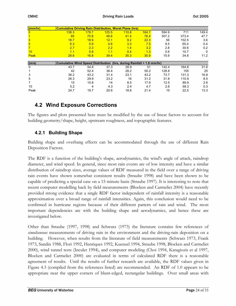
Table 4.1: Summary Annual Driving Rain and Windspeed Statistics
CMHC Driving Rain Loads Oct 2005
BEG University of Waterloo Page 24 of 33
(mm/hr) Cumulative Driving Rain Distribution, Worst Plane (hrs)0 138.3 178.7 125.5 110.8 164.7 594.9 711 149.41 65 70.8 48.6 41.4 76.4 307.2 373.4 47.73 18.7 18.9 12.1 9.2 22.3 56 152.5 3.65 6.3 5.9 4.6 3.3 7.5 9.5 65.4 0.47 2.7 2.3 2.2 1.4 3.2 2.8 30.6 0.210 1.1 0.9 1.1 0.4 1.3 0.6 10.7 0Peak 28.6 16.8 39.4 35.3 30.9 15.9 34.8 11.2 (m/s) Cumulative Wind Speed Distribution (hrs, during Rainfall > 1.8 mm/hr)0 43.7 54.6 37.3 28.9 51 142.4 164.8 31.61 42 52.4 36.4 28.2 50.2 128.8 155 253 36.2 43.2 31.4 23.1 43.2 73.7 131.3 16.85 26.3 29.9 23.2 16 31.2 31.8 110.9 8.57 15 15.8 14 8.5 17.9 12.5 89.9 2.610 5.2 4 4.3 2.4 4.7 2.6 58.3 0.3Peak 24.7 19.7 20.6 18.6 21.4 15 22.5 13.3
4.2 Wind Exposure Corrections The figures and plots presented here must be modified by the use of linear factors to account for building geometry/shape, height, upstream roughness, and topographic features.
4.2.1 Building Shape
Building shape and overhang effects can be accommodated through the use of different Rain Deposition Factors.
The RDF is a function of the building's shape, aerodynamics, the wind's angle of attack, raindrop diameter, and wind speed. In general, since most rain events are of low intensity and have a similar distribution of raindrop sizes, average values of RDF measured in the field over a range of driving rain events have shown somewhat consistent results (Straube 1998) and have been shown to be capable of predicting a special case on a 15 minute basis (Straube 1997). It is interesting to note that recent computer modelling back by field measurements (Blocken and Carmeliet 2004) have recently provided strong evidence that a single RDF factor independent of rainfall intensity is a reasonable approximation over a broad range of rainfall intensities. Again, this conclusion would need to be confirmed in hurricane regions because of their different pattern of rain and wind. The most important dependencies are with the building shape and aerodynamics, and hence these are investigated below.
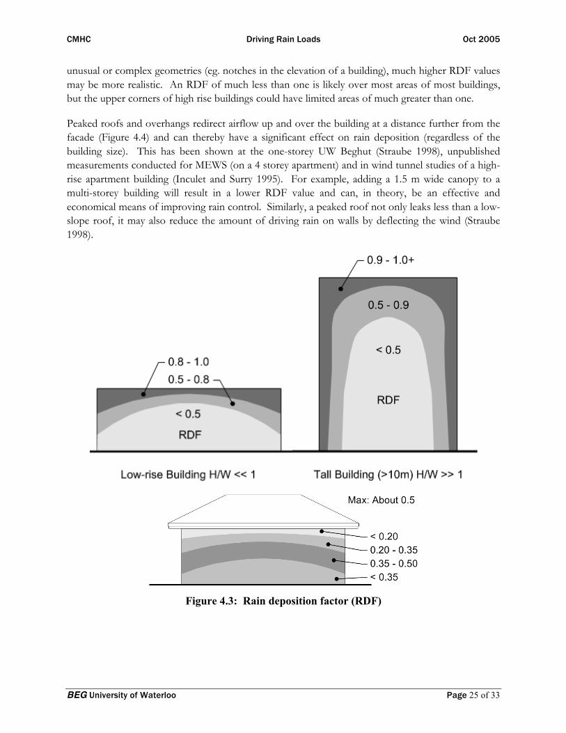
Other than Straube (1997, 1998) and Schwarz (1973) the literature contains few references of simultaneous measurements of driving rain in the environment and the driving-rain deposition on a building. However, when results from the literature of field measurements (Schwarz 1973, Frank 1973, Sandin 1988, Flori 1992, Henriques 1992, Kuenzel 1994, Straube 1998, Blocken and Carmeliet 2000), wind tunnel tests (Inculet 1994), and computer modeling (Choi 1994, Karagiozis et al 1997, Blocken and Carmeliet 2000) are evaluated in terms of calculated RDF there is a reasonable agreement of results. Until the results of further research are available, the RDF values given in Figure 4.3 (compiled from the references listed) are recommended. An RDF of 1.0 appears to be appropriate near the upper corners of blunt-edged, rectangular buildings. Over small areas with
CMHC Driving Rain Loads Oct 2005
BEG University of Waterloo Page 25 of 33
unusual or complex geometries (eg. notches in the elevation of a building), much higher RDF values may be more realistic. An RDF of much less than one is likely over most areas of most buildings, but the upper corners of high rise buildings could have limited areas of much greater than one.
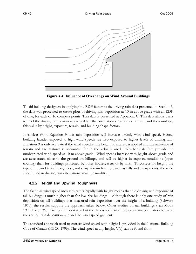
Peaked roofs and overhangs redirect airflow up and over the building at a distance further from the facade (Figure 4.4) and can thereby have a significant effect on rain deposition (regardless of the building size). This has been shown at the one-storey UW Beghut (Straube 1998), unpublished measurements conducted for MEWS (on a 4 storey apartment) and in wind tunnel studies of a high-rise apartment building (Inculet and Surry 1995). For example, adding a 1.5 m wide canopy to a multi-storey building will result in a lower RDF value and can, in theory, be an effective and economical means of improving rain control. Similarly, a peaked roof not only leaks less than a low-slope roof, it may also reduce the amount of driving rain on walls by deflecting the wind (Straube 1998).
Figure 4.3: Rain deposition factor (RDF)
CMHC Driving Rain Loads Oct 2005
BEG University of Waterloo Page 26 of 33
Figure 4.4: Influence of Overhangs on Wind Around Buildings
To aid building designers in applying the RDF factor to the driving rain data presented in Section 3, the data was processed to create plots of driving rain deposition at 10 m above grade with an RDF of one, for each of 16 compass points. This data is presented in Appendix C. This data allows users to read the driving rain, cosine-corrected for the orientation of any specific wall, and then multiply this value by height, exposure, terrain, and building shape factors.
It is clear from Equation 9 that rain deposition will increase directly with wind speed. Hence, building facades exposed to high wind speeds are also exposed to higher levels of driving rain. Equation 9 is only accurate if the wind speed at the height of interest is applied and the influence of terrain and site features is accounted for in the velocity used. Weather data files provide the unobstructed wind speed at 10 m above grade. Wind speeds increase with height above grade and are accelerated close to the ground on hilltops, and will be higher in exposed conditions (open country) than for buildings protected by other houses, trees or by hills. To correct for height, the type of upwind terrain roughness, and sharp terrain features, such as hills and escarpments, the wind speed, used in driving rain calculations, must be modified.
4.2.2 Height and Upwind Roughness
The fact that wind speed increases rather rapidly with height means that the driving rain exposure of tall buildings is much higher than for low-rise buildings. Although there is only one study of rain deposition on tall buildings that measured rain deposition over the height of a building (Schwarz 1973), the results support the approach taken below. Other studies on tall buildings (van Mook 1999, Lacy 1965) have been undertaken but the data is too sparse to capture any correlation between the vertical rain deposition rate and the wind speed gradient.
The standard approach used to correct wind speed with height is provided in the National Building Code of Canada (NBCC 1996). The wind speed at any height, V(z) can be found from:
CMHC Driving Rain Loads Oct 2005
BEG University of Waterloo Page 27 of 33
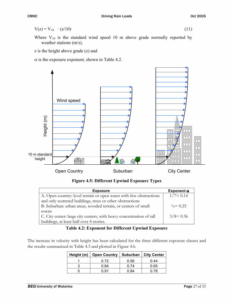
V(z) = V10 · (z/10)α (11)
Where V10 is the standard wind speed 10 m above grade normally reported by weather stations (m/s),
z is the height above grade (z) and
α is the exposure exponent, shown in Table 4.2.
Hei
ght (
m)
Open Country Suburban City Center
Wind speed
10 m standard height
Figure 4.5: Different Upwind Exposure Types
Exposure Exponent α A. Open country: level terrain or open water with few obstructions and only scattered buildings, trees or other obstructions
1/7= 0.14
B. Suburban: urban areas, wooded terrain, or centers of small towns
¼= 0.25
C. City center: large city centers, with heavy concentration of tall buildings, at least half over 4 stories.
3/8= 0.36
Table 4.2: Exponent for Different Upwind Exposure
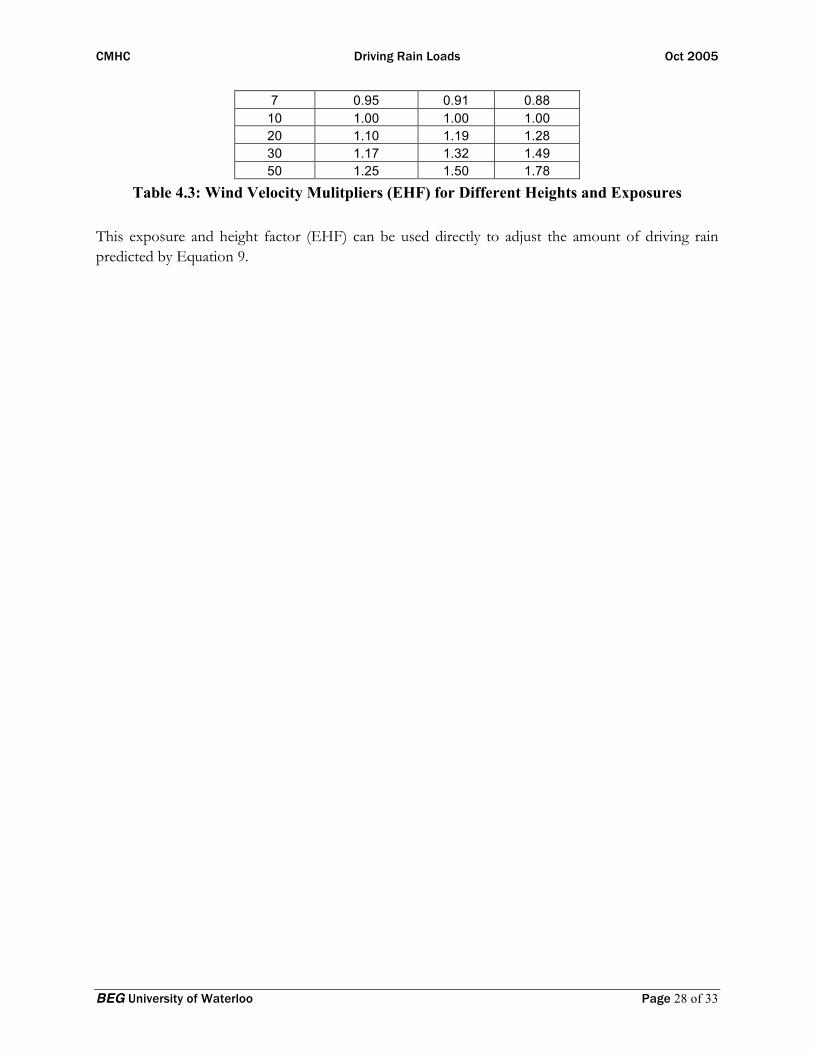
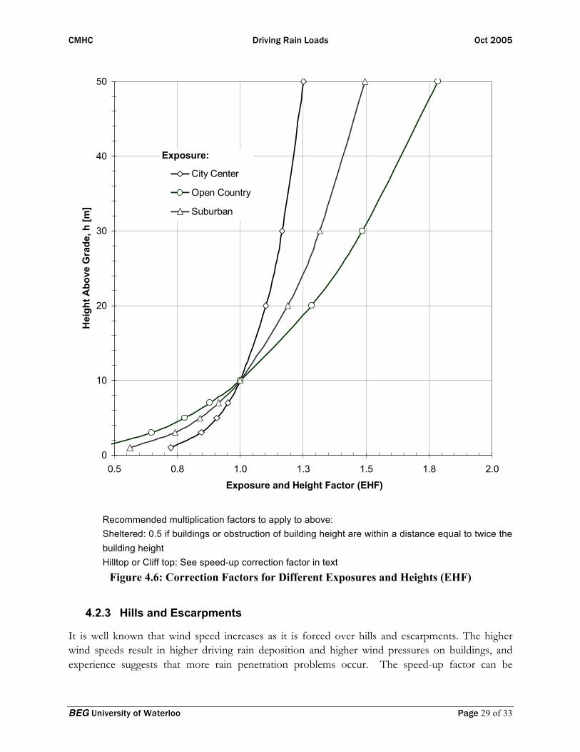
The increase in velocity with height has been calculated for the three different exposure classes and the results summarized in Table 4.3 and plotted in Figure 4.6.
Height (m) Open Country Suburban City Center 1 0.72 0.56 0.44 3 0.84 0.74 0.65 5 0.91 0.84 0.78
CMHC Driving Rain Loads Oct 2005
BEG University of Waterloo Page 28 of 33
7 0.95 0.91 0.88 10 1.00 1.00 1.00 20 1.10 1.19 1.28 30 1.17 1.32 1.49 50 1.25 1.50 1.78
Table 4.3: Wind Velocity Mulitpliers (EHF) for Different Heights and Exposures
This exposure and height factor (EHF) can be used directly to adjust the amount of driving rain predicted by Equation 9.
CMHC Driving Rain Loads Oct 2005
BEG University of Waterloo Page 29 of 33
0
10
20
30
40
50
0.5 0.8 1.0 1.3 1.5 1.8 2.0
Exposure and Height Factor (EHF)
Hei
ght A
bove
Gra
de, h
[m]
City Center
Open Country
Suburban
Exposure:
Recommended multiplication factors to apply to above: Sheltered: 0.5 if buildings or obstruction of building height are within a distance equal to twice the building height Hilltop or Cliff top: See speed-up correction factor in text
Figure 4.6: Correction Factors for Different Exposures and Heights (EHF)
4.2.3 Hills and Escarpments
It is well known that wind speed increases as it is forced over hills and escarpments. The higher wind speeds result in higher driving rain deposition and higher wind pressures on buildings, and experience suggests that more rain penetration problems occur. The speed-up factor can be
CMHC Driving Rain Loads Oct 2005
BEG University of Waterloo Page 30 of 33
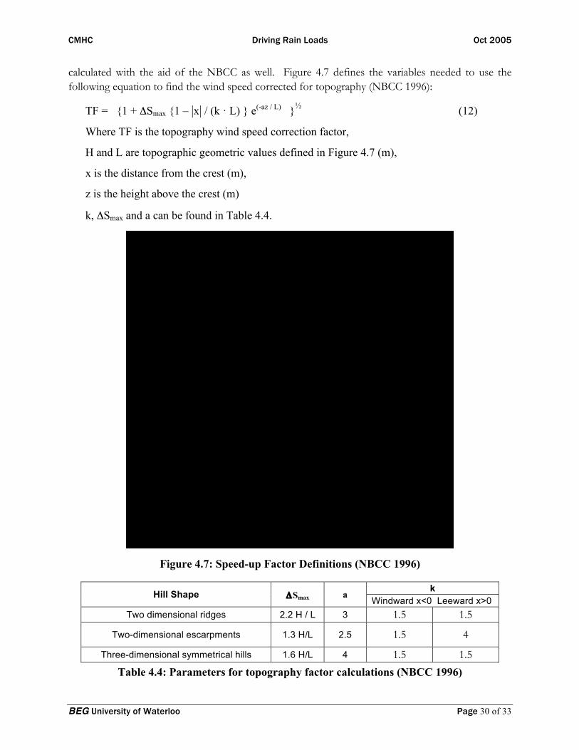
calculated with the aid of the NBCC as well. Figure 4.7 defines the variables needed to use the following equation to find the wind speed corrected for topography (NBCC 1996):
TF = {1 + ΔSmax {1 – |x| / (k · L) } e(-az / L) }½ (12)
Where TF is the topography wind speed correction factor,
H and L are topographic geometric values defined in Figure 4.7 (m),
x is the distance from the crest (m),
z is the height above the crest (m)
k, ΔSmax and a can be found in Table 4.4.
Figure 4.7: Speed-up Factor Definitions (NBCC 1996)
Hill Shape ΔSmax a k Windward x<0 Leeward x>0
Two dimensional ridges 2.2 H / L 3 1.5 1.5
Two-dimensional escarpments 1.3 H/L 2.5 1.5 4
Three-dimensional symmetrical hills 1.6 H/L 4 1.5 1.5
Table 4.4: Parameters for topography factor calculations (NBCC 1996)
CMHC Driving Rain Loads Oct 2005
BEG University of Waterloo Page 31 of 33
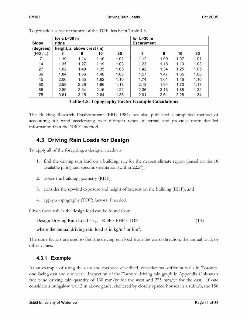
To provide a sense of the size of the TOF has been Table 4.5.
Slope for a L=30 m ridge
for L=30 m Escarpment
(degrees) height, z, above crest (m) (H/2 / L) 3 6 10 30 3 6 10 30
7 1.19 1.14 1.10 1.01 1.12 1.09 1.07 1.01 14 1.35 1.27 1.19 1.03 1.23 1.18 1.13 1.03 27 1.62 1.49 1.35 1.05 1.42 1.34 1.25 1.05 36 1.84 1.66 1.48 1.08 1.57 1.47 1.35 1.08 45 2.06 1.85 1.62 1.10 1.74 1.61 1.46 1.10 60 2.59 2.29 1.96 1.18 2.13 1.94 1.73 1.17 66 2.89 2.54 2.15 1.22 2.36 2.13 1.88 1.22 75 3.61 3.15 2.64 1.35 2.91 2.61 2.28 1.34
Table 4.5: Topography Factor Example Calculations
The Building Research Establishment (BRE 1984) has also published a simplified method of accounting for wind accelerating over different types of terrain and provides more detailed information than the NBCC method.
4.3 Driving Rain Loads for Design To apply all of the foregoing, a designer needs to
1. find the driving rain load on a building, rbv, for the nearest climate region (based on the 18 available plots) and specific orientation (within 22.5°).
2. assess the building geometry (RDF)
3. consider the upwind exposure and height of interest on the building (EHF), and
4. apply a topography (TOF) factors if needed.
Given these values the design load can be found from:
Design Driving Rain Load = rbv · RDF · EHF · TOF (13)
where the annual driving rain load is in kg/m2 or l/m2.
The same factors are used to find the driving rain load from the worst direction, the annual total, or other values.
4.3.1 Example
As an example of using the data and methods described, consider two different walls in Toronto, one facing east and one west. Inspection of the Toronto driving rain graph in Appendix C shows a free wind driving rain quantity of 130 mm/yr for the west and 275 mm/yr for the east. If one considers a bungalow wall 2 m above grade, sheltered by closely spaced houses in a suburb, the 150
CMHC Driving Rain Loads Oct 2005
BEG University of Waterloo Page 32 of 33
mm/yr would be modifying by a factor of 0.7 (from Figure 4.6) and a further reduction factor of 0.5 (from the note on sheltering). If the bungalow had a peaked roof with a 300 mm overhang, an RDF of 0.5 would capture the highest rain values. The result would be a driving rain total of 130*0.7*0.5*0.5= 23 mm per year, which is equivalent to 23 liters per m2 per year.
For an east facing wall on the top floor of a 50 m tall blunt edged (RDF=1.0) condominium in a suburban exposure, Figure provides a correction factor of 1.5. Using and RDF of 1 for the top corners, the driving rain deposition would be predicted to be 275 * 1.5 * 1.0 * 1.0 = 412 mm per year or 412 l/m2/year – almost 20 times as much rain as the sheltered low-rise bungalow wall facing west.
This example demonstrates the very significant influence of exposure and orientation in a climate. It should also be noted that the combination of high exposure and choice of building shape (high RDF) in a low driving rain climate (such as Edmonton) can result in much more rain deposition than a sheltered low rise building in a high driving rain climate (such as Vancouver).
5 CONCLUSIONS Hourly weather data from several sources has been combined to create weather files of hourly wind, wind speed, and rainfall for 18 cities for the period of 1965 to 1989 inclusive. This data was used to calculate climate statistics and driving rain. A methodology for calculating the driving rain load on buildings has been presented and explained.
It is clear that the many complexities of real buildings and sites will render the methodology suggested here inaccurate. However, the method should allow one to generate a reasonable estimate, and to compare one site and building to another on a relative scale. Also, as has been shown, rainfall and wind vary considerably from year to year. Hence, the practical need for a high level of accuracy is questionable.
These data and methodology, although partially validated through field measurements, should be used with care and professional judgment. Many more field measurements of tall and complex building shapes are needed, as are measurements in a range of exposure conditions.
Sincerely,
Dr John Straube Assistant Professor Dept of Civil Engineering and School of Architecture University of Waterloo
CMHC Driving Rain Loads Oct 2005
BEG University of Waterloo Page 33 of 33
6 REFERENCES AES. Software Implementation for Climatological Ice Accretion Modeling Project, Internal Report to Energy and Industrial Applications Section, Atmospheric Environment Service, Canadian Climate Center, Toronto, Canada, 1984.
Barry, R.G., and Chorley, R.J., Atmosphere Weather and Climate, 6 ed., Routledge, New York, 1992.
Beard, K.V., "Terminal Velocity and Shape of Cloud and Precipitation Drops Aloft", J. of the Atmospheric Sciences, Vol. 33, 1976, pp. 851-864.
Best, A.C., "The Size Distribution of Raindrops", Quart. J. Royal Meteor. Soc., Vol. 76, 1950, pp. 16-36.
Blocken, B., Carmeliet, J. “A Simplified Approach for Quantifying Driving Rain on Buildings”, Proc. Of Performance of Exterior Envelopes of Whole Buildings IX, Clearwater, Dec. 2004.
Blocken, B., Carmeliet, J., “Driving Rain on Building Envelopes I: Numerical estimation and Full-scale Experimental Verification”, J. of Thermal Envelope and Building Science Vol 24, No. 1, 2000, pp. 61-85.
Boyd, D.W., “Driving-Rain Map of Canada”, DBR/National Research Council, TN 398, Ottawa, 1963.
Bradley, S.G., and Stow, C.D., "The Measurement of Charge and Size of Raindrops: Part II. Results and Analysis at Ground Level", J. of Appl. Meteor., Vol 13, Feb 1974, pp. 131 - 147.
BRE, The Assessment of Wind Speed over Topography. Digest 283, Building Research Establishment, Garston, U.K, March 1984.
Caton, P.G., "A study of the raindrop-size distributions in the free atmosphere", Quart. J. Royal Meteor. Soc., Vol 92, 1966, pp. 15-30.
Choi, E.C.C., “Simulation of Wind-Driven Rain Around a Building”, Journal of Wind Engineering and Industrial Aerodynamics, Vol 46-47, 1993, pp. 721-729.
Choi, E.C.C.. Determination of the wind-driven-rain intensity on building faces. Journal of Wind Engineering and Industrial Aerodynamics, Vol 51, 1994, pp. 55-69.
Dingle, A.N. and Hardy, K.R., "The description of rain by means of sequential rainddrop-size distributions", Quart. J. Royal Meteor. Soc., Vol. 88, 1962, pp. 301-314.
Dingle, A.N., and Lee, Y., "Terminal Fall Speeds of Raindrops", J. of Appl. Meteor., Vol 11, August 1972, pp. 877 - 879.
Flori, J-P., Influence des Conditions Climatiques sur le Mouillage et le sechalge d'une Facade Vertical. Cahiers du CTSB 2606, September, 1992.
Frank, W., Entwicklung von Regen and Wind auf Gebaeudefassaden, Verlag Ernst & Sohn, Berichte aus der Bauforschung, Vol 86, 1973 pp. 17-40.
Grimm, C.T., "A Driving Rain Index for Masonry Walls", Masonry: Materials, Properties, and Performance, ASTM STP 778, J.G. Borchelt, Ed., American Society of Testing and Materials, 1982, pp. 171-177.
Gunn, R, and Kinzer, G.D., "The terminal velocity of fall for water drops in stagnant air", J. Meteor., Vol 6, 1949 pp. 243-248.
CMHC Driving Rain Loads Oct 2005
BEG University of Waterloo Page 34 of 33
Handbook on the Principles of Hydrology, ed. Donald M. Grey, National Research Council of Canada, Ottawa, 1970, pp. 2.2-2.3.
Henriques, F.M.A.. "Quantification of wind-driven rain - an experimental approach", Building Research and Information, Vol. 20, No. 5, 1992, pp. 295-297.
Inculet, D. and Surry, D.. Simulation of Wind Driven Rain and Wetting Patterns on Buildings. A report published by the CMHC, February 1995.
Karagiozis, A., and Hadjisophocieous, G.,”Wind-Driven Rain on High-Rise Buildings”, Proc. of the BETEC/DOE/ASHRAE Thermal Performance of Building Envelopes VI, Dec. 1995, pp. 399-406.
Karagiozis, A., Hadjisophocieous, G., and Cao, S., "Wind-Driven Rain Distributions on Two Buildings", J. of Wind Engineering and Industrial Aerodynamics, Vol 67 and 68, 1997, pp. 559-572.
Künzel, H.M.. Regendaten für Berechnung des Feuchtetransports, Fraunhofer Institut für Bauphysik, Mitteilung 265, 1994.
Lacasse, M. A., O’Connor, T.J., Nunes, S., Beaulieu, P. 2003. Experimental Assessment of Water Penetration and Entry into Wood-Frame Wall Specimens - Final Report. MEWS Consortium, IRC/NRCC,Ottawa, February, 2003.
Lacy, R.E., “Driving-Rain Maps and the Onslaught of Rain on Buildings”, Proc. of RILEM/CIB Symposium on Moisture Problems in Buildings, Helsinki, (Building Research Station Current Paper 54, HMSO Garston, U.K) 1965.
Laws, J.O., and Parsons, D.A., "Relation of raindrop size to intensity", American Geophys. Union Trans., No. 24, pt. 2, 1943, pp. 453-460.
Levelton Engineering, Wind-Rain Relationships in Southwestern British Columbia – Final Report. Research report for CMHC, Ottawa, August 2004.
Markowitz, A.M., "Raindrop Size Distribution Expressions", J. of Applied Meteorology, Vol. 15, 1976, pp. 1029-1031.
Marshall, J. S., and Palmer, W. M., "The distribution of raindrops with size", J of Meteor., Vol. 5, Aug. 1948, pp.165-166.
NBCC, Users Guide -to National Building Code of Canada 1995 Structural Commentaries (Part 4). Canadian Commission on Building and Fire Codes, National Research Council, Canada,1996.
Rain Penetration Control Guide. CMHC Report, Ottawa, 2000.
Rogers, R.R., and Pilie, R.J.,"Radar Measurements of Drop-Size Distribution", J. of the Atmospheric Sciences, Vol 10, Nov. 1962, pp. 503-506.
Sandin, K., “The Moisture Conditions in Aerated Lightweight Concrete Walls”. Proc. of Symposium and Day of Building Physics, Lund University, Swedish Council for Building Research 1988, pp. 216-220..
Schwarz, B., Witterungsbeansphruchung von Hochhausfassaden. HLH Bd. 24, Nr. 12, 1973, pp. 376-384.
Skerlj, P.F., A Critical Assessment of the Driving Rain Wind Pressures Used in CSA Standard CAN/CSA-A44-M90. M.A.Sc. Thesis, Faculty of Engineering Science, University of Western Ontario, London, Canada, 1999.
Straube, J.F. Burnett, E.F.P., "Rain Control and Design Strategies". J. of Thermal Insulation and Building Envelopes, July, 1999, pp. 41-56.
CMHC Driving Rain Loads Oct 2005
BEG University of Waterloo Page 35 of 33
Straube, J.F. Moisture Control and Enclosure Wall Systems. Ph.D. Thesis, Civil Engineering Department, University of Waterloo, Waterloo, Canada, 1998.
Straube, J.F., Burnett, E.F.P. "Driving Rain and Masonry Veneer", Water Leakage Through Building Facades, ASTM STP 1314, R.J. Kudder and J.L. Erdly, Eds., American Society for Testing and Materials, Philadelphia, 1997, pp. 73-87.
Straube, J.F., Burnett, E.F.P., “Rain Control and Screened Walls”, Proc. of the 7th CSCE Building Science and Technology Conference, Toronto, March, 1997, pp. 17-38.
Straube, J.F., Burnett, E.F.P.. "Pressure Moderation and Rain Control for Multi-Wythe Masonry Walls". Proc of International Building Physics Conference , Eindhoven, September 18-21, 2000, pp. 179-186.
Surry, D., Skerlj, P. , Mikitiuk, M.J., An Exploratory Study of the Climatic Relationships between Rain and Wind, (Final Report BLWT-SS22-1994, Faculty of Engineering Science, University of Western Ontario), CMHC Research Report, Ottawa, February 1995.
Van Mook, F.J.. “Measurements and simulations of driving rain on the main building of the TUE” Proc. Of 5th Symposium on Building Physics in the Nordic Countries, Goteborg, Sweden, August, 1999, pp. 377-384.
Welsh, L.E., Skinner,, W.R., and Morris, R.J., A Climatology of Driving Rain Wind Pressures for Canada. Climate and Atmospheric Research Directorate, Draft Report, Environment Canada, Canada, 1989.
Wisse, J.A., “Driving Rain a numerical study”, Proc. Of 9th Symp. On Building Physics and Building Climatology, Dresden, Germany, Sept. 1994.
BEG University of Waterloo Page A1
Appendix A: Weather Data sources
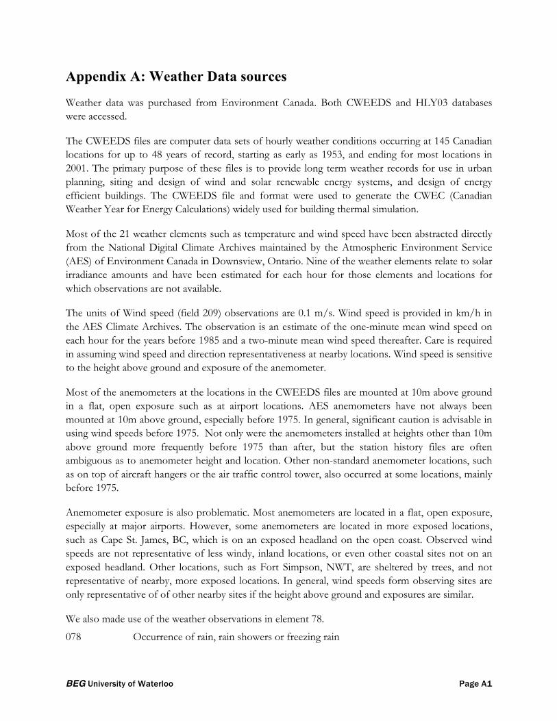
Weather data was purchased from Environment Canada. Both CWEEDS and HLY03 databases were accessed.
The CWEEDS files are computer data sets of hourly weather conditions occurring at 145 Canadian locations for up to 48 years of record, starting as early as 1953, and ending for most locations in 2001. The primary purpose of these files is to provide long term weather records for use in urban planning, siting and design of wind and solar renewable energy systems, and design of energy efficient buildings. The CWEEDS file and format were used to generate the CWEC (Canadian Weather Year for Energy Calculations) widely used for building thermal simulation.
Most of the 21 weather elements such as temperature and wind speed have been abstracted directly from the National Digital Climate Archives maintained by the Atmospheric Environment Service (AES) of Environment Canada in Downsview, Ontario. Nine of the weather elements relate to solar irradiance amounts and have been estimated for each hour for those elements and locations for which observations are not available.
The units of Wind speed (field 209) observations are 0.1 m/s. Wind speed is provided in km/h in the AES Climate Archives. The observation is an estimate of the one-minute mean wind speed on each hour for the years before 1985 and a two-minute mean wind speed thereafter. Care is required in assuming wind speed and direction representativeness at nearby locations. Wind speed is sensitive to the height above ground and exposure of the anemometer.
Most of the anemometers at the locations in the CWEEDS files are mounted at 10m above ground in a flat, open exposure such as at airport locations. AES anemometers have not always been mounted at 10m above ground, especially before 1975. In general, significant caution is advisable in using wind speeds before 1975. Not only were the anemometers installed at heights other than 10m above ground more frequently before 1975 than after, but the station history files are often ambiguous as to anemometer height and location. Other non-standard anemometer locations, such as on top of aircraft hangers or the air traffic control tower, also occurred at some locations, mainly before 1975.
Anemometer exposure is also problematic. Most anemometers are located in a flat, open exposure, especially at major airports. However, some anemometers are located in more exposed locations, such as Cape St. James, BC, which is on an exposed headland on the open coast. Observed wind speeds are not representative of less windy, inland locations, or even other coastal sites not on an exposed headland. Other locations, such as Fort Simpson, NWT, are sheltered by trees, and not representative of nearby, more exposed locations. In general, wind speeds form observing sites are only representative of of other nearby sites if the height above ground and exposures are similar.
We also made use of the weather observations in element 78.
078 Occurrence of rain, rain showers or freezing rain

CMHC Driving Rain Loads Oct 2005
BEG University of Waterloo Page A2
0 = None 1 = Light rain 2 = Moderate rain 3 = Heavy rain 4 = Light rain showers 5 = Moderate rain showers 6 = Heavy rain showers 7 = Light freezing rain 8 = Moderate or heavy freezing rain
We also wish to acknowledge the help provided by Maria Petrou, Data Specialist, National Archives Data Management, Atmospheric Monitoring & Water Survey Directorate, Meteorological Service of Canada, Environment Canada

BEG University of Waterloo Page B1
Appendix B: Climate Statistics including Driving Rain
CMHC Driving Rain Loads Oct 2005
BEG University of Waterloo Page D2
Calgary, AB Driving Rain (mm/yr)
0
25
50
75
100
125
150N
NNE
NE
ENE
E
ESE
SE
SSE
S
SSW
SW
WSW
W
WNW
NW
NNW
For an unobstructured plane perpendicular to wind at 10 m above grade.
Charlottetown, PEI Driving Rain (mm/yr)
0
20
40
60
80
100
120
140
160
180N
NNE
NE
ENE
E
ESE
SE
SSE
S
SSW
SW
WSW
W
WNW
NW
NNW
For an unobstructured plane perpendicular to wind at 10 m above grade.
CMHC Driving Rain Loads Oct 2005
BEG University of Waterloo Page D3
Edmonton, AB Driving Rain (mm/yr)
0
25
50
75
100
125
150N
NNE
NE
ENE
E
ESE
SE
SSE
S
SSW
SW
WSW
W
WNW
NW
NNW
For an unobstructured plane perpendicular to wind at 10 m above grade.
Fredericton, NB Driving Rain (mm/yr)
0
25
50
75
100
125
150N
NNE
NE
ENE
E
ESE
SE
SSE
S
SSW
SW
WSW
W
WNW
NW
NNW
For an unobstructured plane perpendicular to wind at 10 m above grade.
CMHC Driving Rain Loads Oct 2005
BEG University of Waterloo Page D4
Winnipeg, MB Driving Rain (mm/yr)
05101520253035404550
N
NNE
NE
ENE
E
ESE
SE
SSE
S
SSW
SW
WSW
W
WNW
NW
NNW
For an unobstructured plane perpendicular to wind at 10 m above grade.
Montreal, QC Driving Rain (mm/yr)
0
25
50
75
100
125
150N
NNE
NE
ENE
E
ESE
SE
SSE
S
SSW
SW
WSW
W
WNW
NW
NNW
For an unobstructured plane perpendicular to wind at 10 m above grade.
CMHC Driving Rain Loads Oct 2005
BEG University of Waterloo Page D5
North Bay, ON Driving Rain (mm/yr)
0
25
50
75
100
125
150N
NNE
NE
ENE
E
ESE
SE
SSE
S
SSW
SW
WSW
W
WNW
NW
NNW
For an unobstructured plane perpendicular to wind at 10 m above grade.
Ottawa, ON Driving Rain (mm/yr)
0
25
50
75
100
125
150N
NNE
NE
ENE
E
ESE
SE
SSE
S
SSW
SW
WSW
W
WNW
NW
NNW
For an unobstructured plane perpendicular to wind at 10 m above grade.
CMHC Driving Rain Loads Oct 2005
BEG University of Waterloo Page D6
PrinceGeorge, BC Driving Rain (mm/yr)
0
25
50
75
100
125
150N
NNE
NE
ENE
E
ESE
SE
SSE
S
SSW
SW
WSW
W
WNW
NW
NNW
For an unobstructured plane perpendicular to wind at 10 m above grade.
Quebec, QC Driving Rain (mm/yr)
0
50
100
150
200
250
300N
NNE
NE
ENE
E
ESE
SE
SSE
S
SSW
SW
WSW
W
WNW
NW
NNW
For an unobstructured plane perpendicular to wind at 10 m above grade.

CMHC Driving Rain Loads Oct 2005
BEG University of Waterloo Page D7
SaintJohn, NB Driving Rain (mm/yr)
0
50
100
150
200
250N
NNE
NE
ENE
E
ESE
SE
SSE
S
SSW
SW
WSW
W
WNW
NW
NNW
For an unobstructured plane perpendicular to wind at 10 m above grade.
Saskatoon, SK Driving Rain (mm/yr)
0
10
20
30
40
50N
NNE
NE
ENE
E
ESE
SE
SSE
S
SSW
SW
WSW
W
WNW
NW
NNW
For an unobstructured plane perpendicular to wind at 10 m above grade.
CMHC Driving Rain Loads Oct 2005
BEG University of Waterloo Page D8
Shearwater, NS Driving Rain (mm/yr)
0
50
100
150
200
250
300
350N
NNE
NE
ENE
E
ESE
SE
SSE
S
SSW
SW
WSW
W
WNW
NW
NNW
For an unobstructured plane perpendicular to wind at 10 m above grade.
St Johns, NF Driving Rain (mm/yr)
0
50
100
150
200
250
300
350N
NNE
NE
ENE
E
ESE
SE
SSE
S
SSW
SW
WSW
W
WNW
NW
NNW
For an unobstructured plane perpendicular to wind at 10 m above grade.
CMHC Driving Rain Loads Oct 2005
BEG University of Waterloo Page D9
Sydney, NS Driving Rain (mm/yr)
0
50
100
150
200
250
300N
NNE
NE
ENE
E
ESE
SE
SSE
S
SSW
SW
WSW
W
WNW
NW
NNW
For an unobstructured plane perpendicular to wind at 10 m above grade.
Toronto ON Driving Rain (mm/yr)
0
25
50
75
100
125
150N
NNE
NE
ENE
E
ESE
SE
SSE
S
SSW
SW
WSW
W
WNW
NW
NNW
For an unobstructured plane perpendicular to wind at 10 m above grade.
CMHC Driving Rain Loads Oct 2005
BEG University of Waterloo Page D10
Vancouver, BC Driving Rain (mm/yr)
0
100
200
300
400
500N
NNE
NE
ENE
E
ESE
SE
SSE
S
SSW
SW
WSW
W
WNW
NW
NNW
For an unobstructured plane perpendicular to wind at 10 m above grade.
Winnipeg, MB Driving Rain (mm/yr)
05101520253035404550
N
NNE
NE
ENE
E
ESE
SE
SSE
S
SSW
SW
WSW
W
WNW
NW
NNW
For an unobstructured plane perpendicular to wind at 10 m above grade.
BEG University of Waterloo Page C1
Appendix C: Driving Rain on Vertical Building Surfaces
CMHC Driving Rain Loads Oct 2005
BEG University of Waterloo Page D2
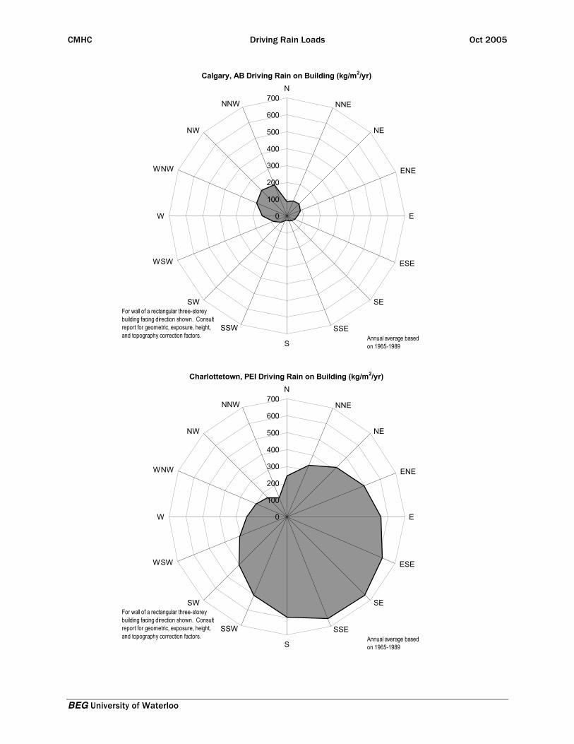
Calgary, AB Driving Rain on Building (kg/m2/yr)
0
100
200
300
400
500
600
700N
NNE
NE
ENE
E
ESE
SE
SSE
S
SSW
SW
WSW
W
WNW
NW
NNW
For wall of a rectangular three-storey building facing direction shown. Consult report for geometric, exposure, height, and topography correction factors. Annual average based
on 1965-1989
Charlottetown, PEI Driving Rain on Building (kg/m2/yr)
0
100
200
300
400
500
600
700N
NNE
NE
ENE
E
ESE
SE
SSE
S
SSW
SW
WSW
W
WNW
NW
NNW
For wall of a rectangular three-storey building facing direction shown. Consult report for geometric, exposure, height, and topography correction factors. Annual average based
on 1965-1989
CMHC Driving Rain Loads Oct 2005
BEG University of Waterloo Page D3
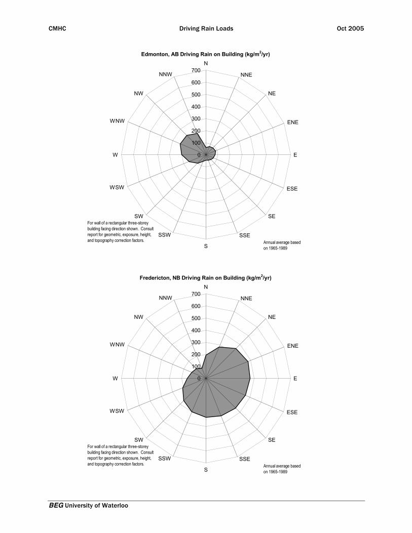
Edmonton, AB Driving Rain on Building (kg/m2/yr)
0
100
200
300
400
500
600
700N
NNE
NE
ENE
E
ESE
SE
SSE
S
SSW
SW
WSW
W
WNW
NW
NNW
For wall of a rectangular three-storey building facing direction shown. Consult report for geometric, exposure, height, and topography correction factors. Annual average based
on 1965-1989
Fredericton, NB Driving Rain on Building (kg/m2/yr)
0
100
200
300
400
500
600
700N
NNE
NE
ENE
E
ESE
SE
SSE
S
SSW
SW
WSW
W
WNW
NW
NNW
For wall of a rectangular three-storey building facing direction shown. Consult report for geometric, exposure, height, and topography correction factors. Annual average based
on 1965-1989
CMHC Driving Rain Loads Oct 2005
BEG University of Waterloo Page D4
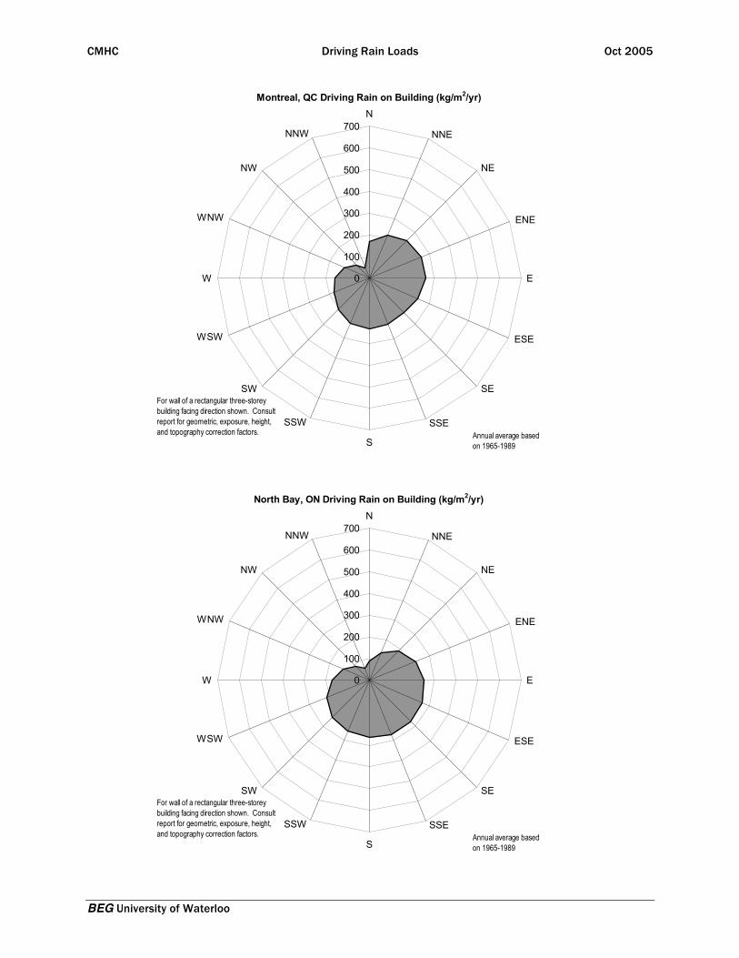
Montreal, QC Driving Rain on Building (kg/m2/yr)
0
100
200
300
400
500
600
700N
NNE
NE
ENE
E
ESE
SE
SSE
S
SSW
SW
WSW
W
WNW
NW
NNW
For wall of a rectangular three-storey building facing direction shown. Consult report for geometric, exposure, height, and topography correction factors. Annual average based
on 1965-1989
North Bay, ON Driving Rain on Building (kg/m2/yr)
0
100
200
300
400
500
600
700N
NNE
NE
ENE
E
ESE
SE
SSE
S
SSW
SW
WSW
W
WNW
NW
NNW
For wall of a rectangular three-storey building facing direction shown. Consult report for geometric, exposure, height, and topography correction factors. Annual average based
on 1965-1989
CMHC Driving Rain Loads Oct 2005
BEG University of Waterloo Page D5
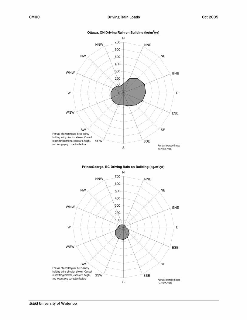
Ottawa, ON Driving Rain on Building (kg/m2/yr)
0
100
200
300
400
500
600
700N
NNE
NE
ENE
E
ESE
SE
SSE
S
SSW
SW
WSW
W
WNW
NW
NNW
For wall of a rectangular three-storey building facing direction shown. Consult report for geometric, exposure, height, and topography correction factors. Annual average based
on 1965-1989
PrinceGeorge, BC Driving Rain on Building (kg/m2/yr)
0
100
200
300
400
500
600
700N
NNE
NE
ENE
E
ESE
SE
SSE
S
SSW
SW
WSW
W
WNW
NW
NNW
For wall of a rectangular three-storey building facing direction shown. Consult report for geometric, exposure, height, and topography correction factors. Annual average based
on 1965-1989
CMHC Driving Rain Loads Oct 2005
BEG University of Waterloo Page D6
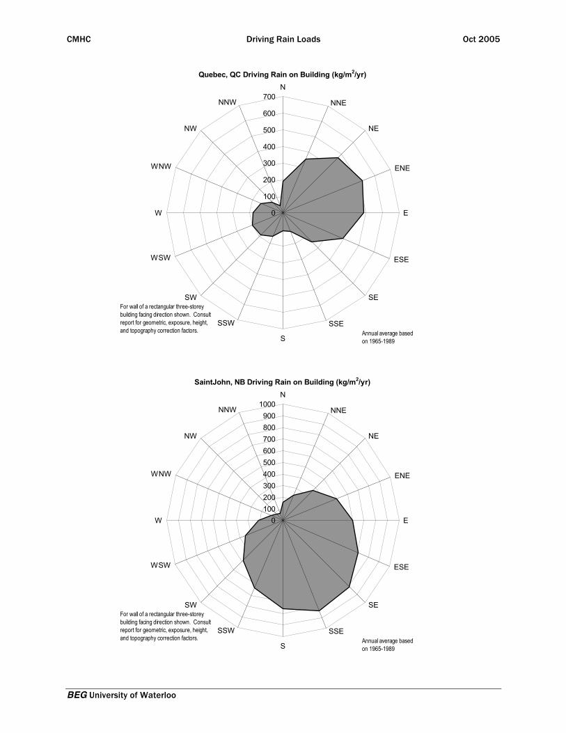
Quebec, QC Driving Rain on Building (kg/m2/yr)
0
100
200
300
400
500
600
700N
NNE
NE
ENE
E
ESE
SE
SSE
S
SSW
SW
WSW
W
WNW
NW
NNW
For wall of a rectangular three-storey building facing direction shown. Consult report for geometric, exposure, height, and topography correction factors. Annual average based
on 1965-1989
SaintJohn, NB Driving Rain on Building (kg/m2/yr)
01002003004005006007008009001000
N
NNE
NE
ENE
E
ESE
SE
SSE
S
SSW
SW
WSW
W
WNW
NW
NNW
For wall of a rectangular three-storey building facing direction shown. Consult report for geometric, exposure, height, and topography correction factors. Annual average based
on 1965-1989
CMHC Driving Rain Loads Oct 2005
BEG University of Waterloo Page D7
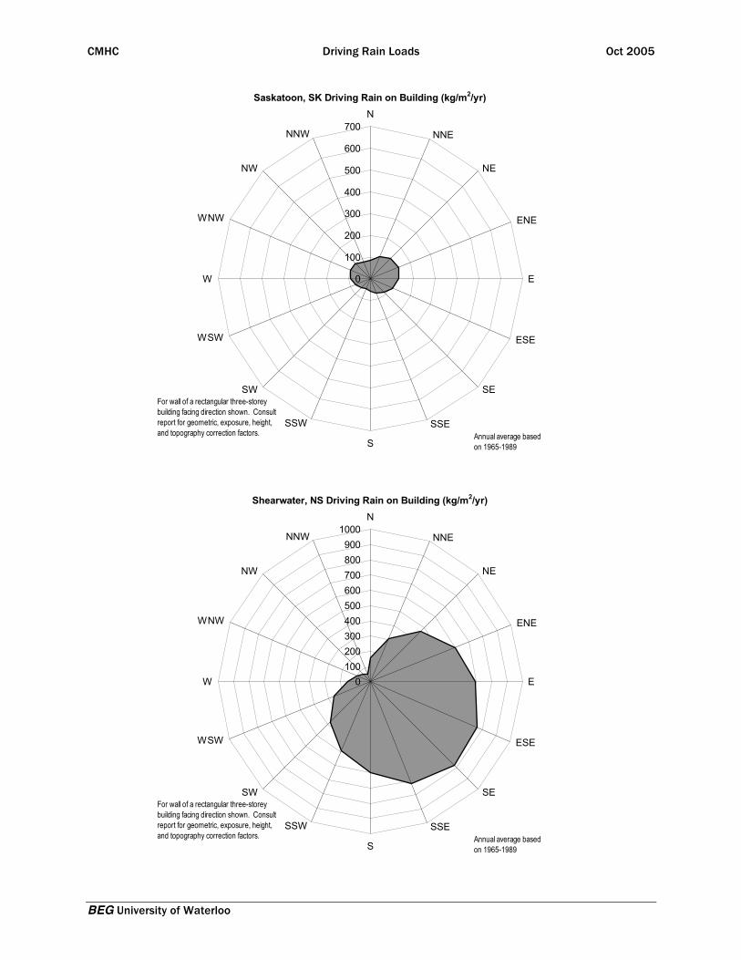
Saskatoon, SK Driving Rain on Building (kg/m2/yr)
0
100
200
300
400
500
600
700N
NNE
NE
ENE
E
ESE
SE
SSE
S
SSW
SW
WSW
W
WNW
NW
NNW
For wall of a rectangular three-storey building facing direction shown. Consult report for geometric, exposure, height, and topography correction factors. Annual average based
on 1965-1989
Shearwater, NS Driving Rain on Building (kg/m2/yr)
01002003004005006007008009001000
N
NNE
NE
ENE
E
ESE
SE
SSE
S
SSW
SW
WSW
W
WNW
NW
NNW
For wall of a rectangular three-storey building facing direction shown. Consult report for geometric, exposure, height, and topography correction factors. Annual average based
on 1965-1989
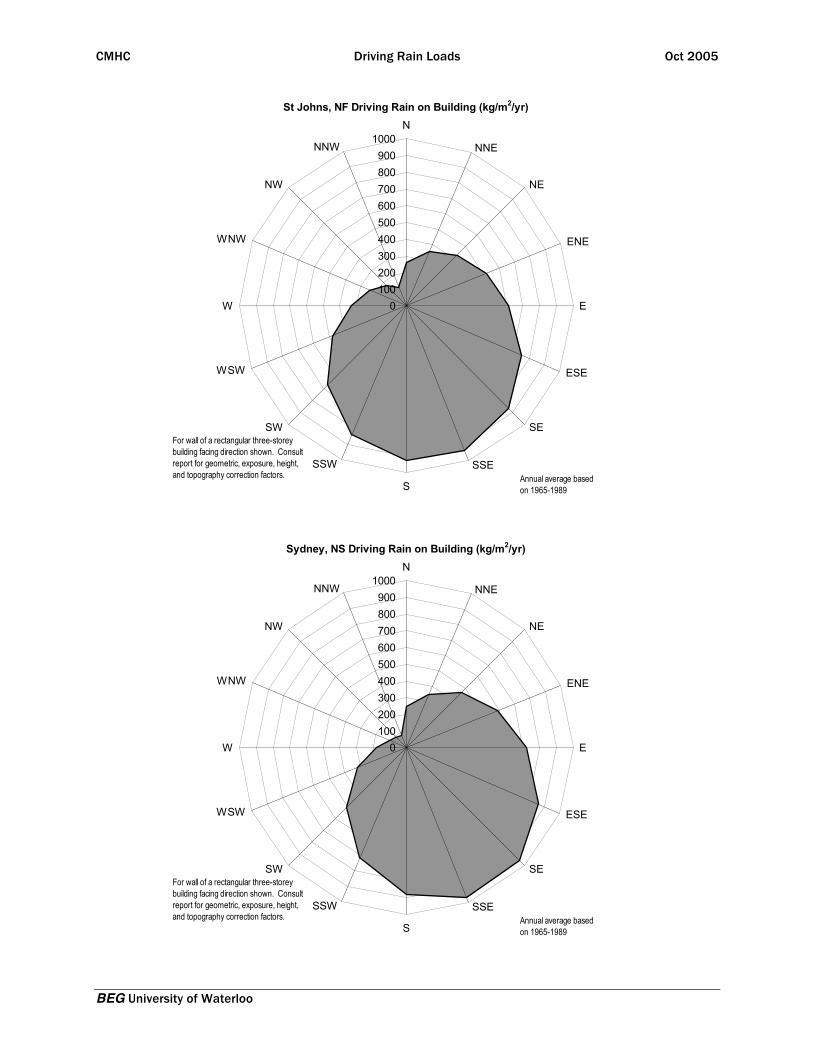
CMHC Driving Rain Loads Oct 2005
BEG University of Waterloo Page D8
St Johns, NF Driving Rain on Building (kg/m2/yr)
01002003004005006007008009001000
N
NNE
NE
ENE
E
ESE
SE
SSE
S
SSW
SW
WSW
W
WNW
NW
NNW
For wall of a rectangular three-storey building facing direction shown. Consult report for geometric, exposure, height, and topography correction factors. Annual average based
on 1965-1989
Sydney, NS Driving Rain on Building (kg/m2/yr)
01002003004005006007008009001000
N
NNE
NE
ENE
E
ESE
SE
SSE
S
SSW
SW
WSW
W
WNW
NW
NNW
For wall of a rectangular three-storey building facing direction shown. Consult report for geometric, exposure, height, and topography correction factors. Annual average based
on 1965-1989
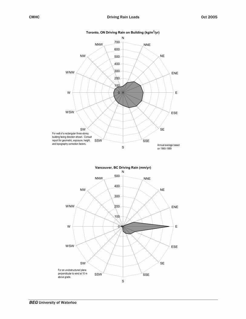
CMHC Driving Rain Loads Oct 2005
BEG University of Waterloo Page D9
Toronto, ON Driving Rain on Building (kg/m2/yr)
0
100
200
300
400
500
600
700N
NNE
NE
ENE
E
ESE
SE
SSE
S
SSW
SW
WSW
W
WNW
NW
NNW
For wall of a rectangular three-storey building facing direction shown. Consult report for geometric, exposure, height, and topography correction factors. Annual average based
on 1965-1989
Vancouver, BC Driving Rain (mm/yr)
0
100
200
300
400
500N
NNE
NE
ENE
E
ESE
SE
SSE
S
SSW
SW
WSW
W
WNW
NW
NNW
For an unobstructured plane perpendicular to wind at 10 m above grade.
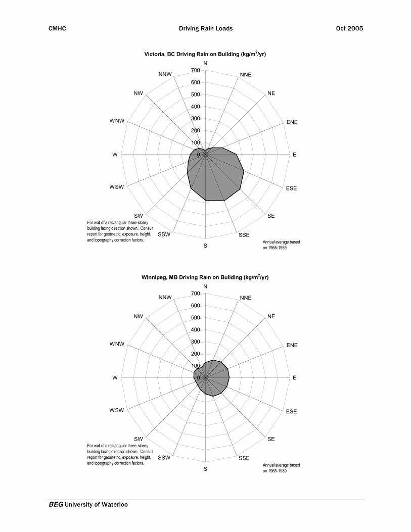
CMHC Driving Rain Loads Oct 2005
BEG University of Waterloo Page D10
Victoria, BC Driving Rain on Building (kg/m2/yr)
0
100
200
300
400
500
600
700N
NNE
NE
ENE
E
ESE
SE
SSE
S
SSW
SW
WSW
W
WNW
NW
NNW
For wall of a rectangular three-storey building facing direction shown. Consult report for geometric, exposure, height, and topography correction factors. Annual average based
on 1965-1989
Winnipeg, MB Driving Rain on Building (kg/m2/yr)
0
100
200
300
400
500
600
700N
NNE
NE
ENE
E
ESE
SE
SSE
S
SSW
SW
WSW
W
WNW
NW
NNW
For wall of a rectangular three-storey building facing direction shown. Consult report for geometric, exposure, height, and topography correction factors. Annual average based
on 1965-1989