Embed Size (px)
Citation preview

DRIVERS OF THE MARKET
1

About us
.
2
Incorporated in 1982, Raine & Horne International Zaki + Partners Sdn.
Bhd. is a firm of Chartered Surveyors and Registered Valuers. Our practice
covers a wide range of services including property valuation, investment and
project management, property management, real estate agency and
property consultancy.
The firm currently operates twelve (12) offices in Malaysia: Kuala Lumpur,
Petaling Jaya, Subang Jaya, Kelang, Johor Bahru, Melaka, Ipoh, Seremban,
Kuantan, Penang, Kota Kinabalu and Kuching.
Since its inception and establishment, Raine & Horne International Zaki +
Partners Sdn. Bhd. has enjoyed an outstanding and enviable reputation and
success. The firm has received wide recognition from all quarters, nationally
and internationally.
Founded in 1883, Raine & Horne is one of the world’s largest real estate
organisations with offices and affiliates all over the world, including in the
major cities of South East Asia, Europe, Canada, USA, Fiji, Australia, New
Zealand, Japan and Africa.
Raine & Horne International Zaki + Partners Sdn. Bhd. aims to provide our
clients with quality professional service. Raine & Horne International Zaki +
Partners Sdn. Bhd. is committed to the Quality Management System required by
ISO 9001:2008 Standards.
Our team comprises of highly qualified partners in various expertise which
authorize us to offer broad ranges of services in:
Professional Valuation Services
Corporate Advisory Services
Project Management
Property Management & Maintenance
Real Estate Agency
Auctioning
Market Research & Feasibility Studies
Property Investment Consultancy
Building Auditing
Bio Asset Valuation
Forensic Valuation
CYF.A5/07.14

Contents
3
Summary………………..........…...........4
Drivers of the Market…………………6
Mortgage Rates………………………...7
Housing costs relative to Income........15
Speculative Activity..............................16
Demographic Factors………………...19
Micro Factors.......................................26
References………………………….....27
Contact us…………………………….29
International Affiliations…………….30
CYF.A5/07.14

Summary
.
4
Classified under the broad category of alternative investments; the real estate
market is inevitably tied to the performance of various economic factors. Such
factors are further refined into macro and micro drivers, which serve as the
determinants of the level of activity in the property market.
Macro Drivers
Some of the more important determinants of the housing sector include:
Mortgage rates
In general, mortgage rates have an inverse relationship with housing activities.
As one rises, the other is expected to fall. Historically, mortgage rate is widely
anticipated to rise in the near future due to various reasons. Such reasons
include the upswing in leading indicators such as US mortgage rates, yield of
10-year MGS, and ticking up of inflation rate.
Contrary, there were arguments against a hike in local interest rates such as the
existence of high level of household debts, elevated debt service ratios, ever
increasing bankruptcy cases, and weakening GDP growth rate. Recent
improvement of the GDP in Q1 2014 backed by strong exports has provided the
perfect opportunity for Bank Negara to raise interest rates.
The degree of the hike will be closely monitored, should the central bank
decides to do so. Since, an increase in interest rates will translate into a stronger
Ringgit and thus putting pressure on exports which currently supports the better
performance of the GDP.
Housing costs relative to Income
Housing price was increasing faster than income for most of the time. This was
more pronounced in recent years. This does not bode well for the property
market in the long run, since affordability of the housing market will be out of
reach for most of the population. Recent cooling policies were necessary to
avoid such radical incident.
Speculative Activity
During the 10-year period being examined, the property market was noticed to
be constantly under speculative influence whether it was positive or negative.
An exception was witnessed in 2013 due to various cooling measures applied.
CYF.A5/07.14
Summary
.
5
A quick view on the KLSE Property Index has provided the affirmation in
which the property market was and still is on an uptrend; with higher support
and higher resistance levels. Trading volumes were strong and supportive of any
surge. Thus, developers were still speculated to perform well over the short and
long-term.
Demographic Factors
Malaysia’s population is aging slowly but still in its early stages. Median age
has increased from 23.6 (2000) to 26.2 (2010); which is still a relatively young
population. Annualized average growth rate has declined slowly throughout the
years. The highest percentage of working adults are in the 20 – 29 age group,
followed by 30 – 39. These 2 groups are ages of greatest household formations.
Malaysia has a low population density ratio coming in at just 86 person/km2.
The nation’s population is not evenly distributed with concentrations in a few
selective states. The degree of density usually dictates the type of houses offered
by developers.
On the other hand, the nation recorded a fairly moderate urbanization rate of
71.0% in 2010. The household size of 4.31 person/household is considered
fairly large on an international standard. It is anticipated that there could be a
high possibility of smaller household size in the future. Such a reduction in the
number of person per household would directly increase the demand for new
living quarters and strain the existing housing stock in the market. In addition,
smaller household size would translate into demand for smaller residential units
as well.
Micro Drivers
As revealed earlier, macro drivers affect the property market at a national scale,
while micro drivers emphasize on local conditions of the subject property.
The price of house is a function of several local variables such as location
characteristics, house characteristics, plot size, surrounding view and
neighbourhood characteristics. These factors usually adhere to a general
guideline but in some instances, may subject to personal preference.
Buyers would be more willing to pay a higher price for the house if these related
characteristics matched their individual expectations and preferencesCYF.A5/07.14

Drivers of the Market
Classified under the broad category of alternative investments; the real estate
market is inevitably tied to the performance of various economic factors. Such
factors are further refined into macro and micro drivers, which serve as the
determinants of the level of activity in the property market.
Macro Drivers
According to Kaplan University (2013), some of the more important
determinants of the housing sector include:
1. Mortgage rates
2. Housing costs relative to income
3. Speculative activity
4. Demographic factors
They are quite similar and do overlap with some of the factors listed under the
expanded equation of hedonic regression by Wheatley (2012):
Ps = W (S, Y, Z)
Ps: price of house
W: willingness to pay
S: size of house
Y: household income
Z: vector (individual preferences; based on age, race, social background, family
size etc.)
In this equation, the price of house is determined by the factors of S, Y, and Z
as stated above.
Micro Drivers
Besides addressing the macro drivers which affect the property market at a
national scale, micro drivers emphasize on local conditions of the subject
property. The main equation of hedonic regression by Wheatley (2012) are as
follow:
P = f (L, T, S, V, N)
P: price of house
f: function of
L: location characteristics
T: house characteristics
S: plot size
V: surrounding view
N: neighbourhood characteristics6CYF.A5/07.14

Mortgage Rates
7
ALR = Malaysia Average Lending Rate
US MR = United States 30-years Mortgage Rate
0.00
1.00
2.00
3.00
4.00
5.00
6.00
7.00
2005 2006 2007 2008 2009 2010 2011 2012 2013 2014
INTE
RST
RA
TE (
%)
10 YRS MEAN (ALR) 10 YRS MEAN (US MR)
Poly. (MALAYSIA ALR) Poly. (US 30-YR MORTGAGE RATE)
The ALR (average lending rate) of Malaysian banks were decreasingthroughout the 10-year period being studied and currently at an all-time low.Low mortgage rate has fuelled the boom of the property market and at the sametime encouraged households to rack in more debts.
When compared to the US 30-year mortgage rate, interest rates were almostcomparable between 2005 to 2009. Divergence begun in the aftermath of thesubprime mortgage crisis. In order to stimulate growth, interest rates in US wasartificially suppressed to historical low in order to promote growth.
Recent improvements in the US labour and housing market have promptedspeculation that interest rates will be raise sooner than expected. This wasreflected in rising mortgage rates and 10-year treasury bonds back in 2013 andcontinuing into 2014. Thus the spread between the Malaysia ALR and US 30-year mortgage rate has narrowed to a small margin. If the long-term trend holds,interest rates in Malaysia will be under pressure to rise.
Figure 1: Mortgage rates in Malaysia and US (BNM, 2014; Freddie Mac, 2014).
CYF.A5/07.14

Mortgage Rates
8
OPR = Overnight policy rate, IBR = Interbank rate
BLR = Base lending rate, ALR = Average lending rate
MGS = Malaysian government securities, FDR = Fixed-deposit rate
The OPR was quite stable in last 10 years, with the exception in 2009 due to the
subprime mortgage crisis. The 3-month IBR and 1-month FDR generally tracks the
OPR set by Bank Negara. Savings rate is currently at an all-time low at 0.25%. This
has boosted the margin of banks and the incentive to lend.
Due to lower payout for savings, banks could lend at a lower rate, this was reflected in
the decreasing ALR compared to the proposed BLR. However, the spread between
ALR and FDR are narrowing, thus squeezing the margin of banks, and their
willingness to lend. If OPR is to rise, FDR will follow suit hence putting pressure on
banks to raise mortgage rates.
Based on the chart above, 10-year MGS is usually a leading indicator of OPR. This
was displayed in 2007, where the 10-year MGS dipped before the drop of OPR in
2009. The 10-year MGS is seen rising again in 2014, pricing in a hike in OPR.
Back in the old days before the subprime mortgage crisis, it makes sense that the
general public withdraw money from the pension fund to pay for mortgage down
payments; due to the reason that the yield of EPF is lower than the ALR. However,
this is no longer true after 2009, where rise in asset prices has caused EPF yields to
overtake mortgage rates. A substantial rise in mortgage rates might just reverse the
current condition.
Figure 2: Interest rates in Malaysia
(BNM, 2014, EPF, 2014; Trading Economics, 2014).
0.00
1.00
2.00
3.00
4.00
5.00
6.00
7.00
8.00
2005 2006 2007 2008 2009 2010 2011 2012 2013 2014
INTE
RES
T R
ATE
(%
)
OPR 3-MONTH IBR BLR ALR
10-YR MGS 1-M FDR SAVINGS RATE EPF YIELD
CYF.A5/07.14

Mortgage Rates
9
Inflation rate
Another reason for the central bank to raise OPR is the ticking up of inflation
rate due to subsidy reduction by government. Anticipation of further subsidy
removal and the implementation of GST in 2015 has fuelled expectations that
the local inflation rate may build up to the 4% level thus causing a negative rate
of return at the current interest level.
However, there are some important considerations before deciding for a hike in
OPR. Under current circumstance, inflation is caused mainly by the removal of
subsidies and not by high growth rate. As such, an excessive hike in OPR might
put downward pressure on the already weakening domestic economy.
Argument against an excessive hike in interest rate will be delivered in the
subsequent pages.
Figure 3: Inflation rate in Malaysia (Trading Economics, 2014).
0.00
1.00
2.00
3.00
4.00
5.00
6.00
2005 2006 2007 2008 2009 2010 2011 2012 2013 2014
INFL
ATI
ON
RA
TE (
%)
INFLATION RATE 10 YRS AVERAGE 3 YRS AVERAGE
CYF.A5/07.14

Mortgage Rates
10
Household debt & Savings rate
The easy monetary policy back in 2009 has seen its effect on interest rates
where ALR and savings rate dropped to record low. This in turn affect the
household debt and savings rate in Malaysia directly.
Due to historical low interest rates, households were tempted to borrow more
and save less. A boom in household debt was witnessed since 2009 and
increasing steadily throughout the years. While gross domestic savings were
below the 40% mark since 2009. This translates into a debt/savings ratio from
around 1.5 (pre-crisis) to 2.0 (after 2009).
An excessive hike in interest rates will therefore weigh on the high level of
existing debts, causing more defaults if the situation runs out of hand.
Figure 4: Household debt and Gross domestic savings in Malaysia (BNM, 2014).
2003.5 2004.5 2005.5 2006.5 2007.5 2008.5 2009.5 2010.5 2011.5 2012.5
0.00
0.50
1.00
1.50
2.00
2.50
0.00
10.00
20.00
30.00
40.00
50.00
60.00
70.00
80.00
90.00
2004 2005 2006 2007 2008 2009 2010 2011 2012
% O
F G
DP
HOUSEHOLD DEBT/GDPGROSS DOMESTIC SAVINGS/GDPHOUSEHOLD DEBT/GROSS DOMESTIC SAVINGS
CYF.A5/07.14

Mortgage Rates
11
Debt servicing
Figure 5 depicts that a lion’s share of the household debts were dedicated
towards the repayment of property loans. Thus, an excessive hike in interest
rates will affect the property market negatively.
Whereas the debt to service ratio was above the 30% proposed guideline; which
is not really healthy. A raise in interest rates will definitely increase the debt to
service ratio above the current level.
Figure 5: Composition of household debt in Malaysia (The Star Online, 2014).
2007 2008 2009 2010 2011 2012
-2.00
-1.00
0.00
1.00
2.00
3.00
4.00
36.00
37.00
38.00
39.00
40.00
41.00
42.00
43.00
44.00
45.00
46.00
2007 2008 2009 2010 2011 2012
YO
Y %
CH
AN
GE
DEB
T SE
RV
ICE
RA
TIO
(%
)
DEBT SERVICE RATIO YOY % CHANGE
Figure 6: Debt to service ratio in Malaysia (BNM, 2014).
CYF.A5/07.14
Mortgage Rates
12
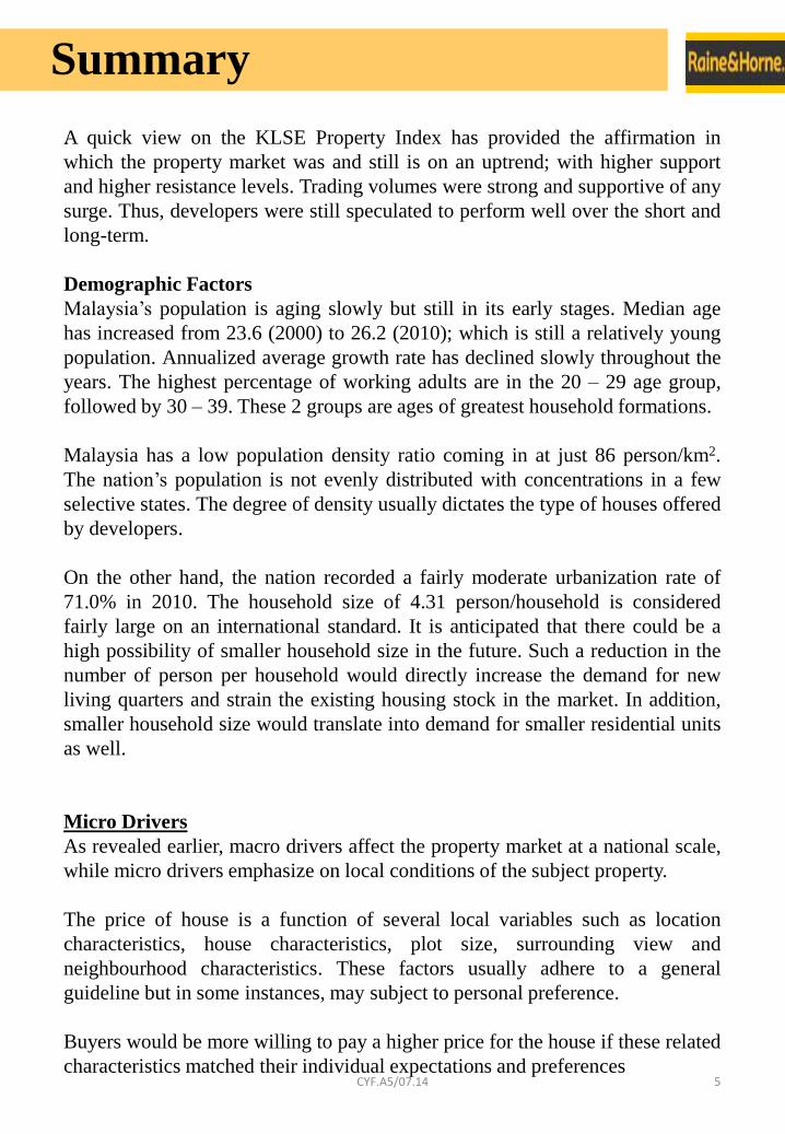
Debt servicing (Cont’d)
Nonetheless, not all situation seemed to be doom and gloom. With the level of
debts pilling up, the quality of loans has equally improved. NPL has been
improving in the last 10 years and is now comparable to those of developed
nations.
On the other hand, bankruptcy rate is at an all-time high and 13% of the cases
were related to housing loans; which is quite a moderate share.
Figure 7: Percentage of Non-performing loans (NPL) to total loans
(Trading Economics, 2014).
Figure 8 & 9: Bankruptcy rate and its components
(The Star Online, 2012; Trading Economics, 2014).
2004 2005 2006 2007 2008 2009 2010 2011 2012 2013
-2.50
-2.00
-1.50
-1.00
-0.50
0.00
0.00
2.00
4.00
6.00
8.00
10.00
12.00
14.00
2004 2005 2006 2007 2008 2009 2010 2011 2012 2013
YO
Y %
CH
AN
GE
NP
L (%
)
NPL YOY % CHANGE 10 YRS AVERAGE 3 YRS AVERAGE
-20.00
0.00
20.00
40.00
2005 2007 2009 2011 2013YO
Y C
HA
NG
E (%
)
BANKRUPTCY RATE (YOY % CHANGE)10 YRS AVERAGE3 YRS AVERAGE
CAR LOANS
25%
OTHER LOANS
21%
PERSONAL LOANS
13%
HOUSING LOANS
13%
BUSINESS LOANS
12%
OTHERS16%
CYF.A5/07.14

Mortgage Rates
13
GDP & Property valueBased on Figure 10, it is noticed that the GDP growth rate of Malaysianeconomy was slowing down. Whereas the growth rate for the construction sub-sector (residential and non-residential) is becoming an important factor tosupport the economy of the country as a whole. Even though the portion of thisconstruction sub-sector is small compared to overall GDP; nonetheless theimmense spillover and multiplication effect of it is important to boost othersectors of the economy.
Whereas the growth rate for total value of property transactions hasoverextended in 2010 and 2011, causing it to revert closer to the nominal GDPgrowth rate. An excessive hike in interest rates will inevitably dent the growthrate of the local economy and definitely is an issue to be concerned over by thecentral bank. Recent improvement of the GDP in Q1 2014 backed by strongexports has provided the perfect opportunity for Bank Negara to raise interestrates.
The degree of the hike will be closely monitored, should the central bankdecides to do so. Since, an increase in interest rates will translate into a strongerRinggit and thus putting pressure on exports which currently supports the betterperformance of the GDP.
Figure 10: YOY changes for GDP, construction sub-sector (residential & non-
residential), and total value of property transactions
(Department of Statistics Malaysia, 2014; JPPH, 2014).
-20.00
-10.00
0.00
10.00
20.00
30.00
40.00
2006 2007 2008 2009 2010 2011 2012 2013
YO
Y %
CH
AN
GE
GDP AT CURRENT PRICES
GDP FOR SUB-SECTOR OF CONSTRUCTION (R & NR)
VALUE OF PROPERTY TRANSACTION
CYF.A5/07.14

Mortgage Rates
14
Construction sector
As mentioned in the previous section, the growth rate of construction sector was
faster than the pace of the overall economy. Further analysis of this sector has
provided the evidence that the growth rate of residential sector has overtaken
non-residential since 2011. Nevertheless, their direct contribution towards the
GDP was insignificant (slightly over 2% of the overall GDP).
An excessive hike in interest rates will most certain hold back this sector due to
the increment in financing cost and reduction in demand appetite for properties.
The current strength witnessed in the construction sector implied that
developers were confident in the outlook of the property market.
Figure 11: GDP of construction sub-sector (residential & non-residential).
(Department of Statistics Malaysia, 2014).2006 2007 2008 2009 2010 2011 2012 2013
-10.00
0.00
10.00
20.00
30.00
40.00
50.00
0.00
0.50
1.00
1.50
2.00
2.50
2006 2007 2008 2009 2010 2011 2012 2013
YOY %
CH
AN
GE
% O
F G
DP
% OF TOTAL GDP (RESIDENTIAL) % OF TOTAL GDP (NON-RESIDENTIAL)
YOY % CHANGE (RESIDENTIAL) YOY % CHANGE (NON-RESIDENTIAL)
CYF.A5/07.14

Housing costs relative to Income
15
GDP per capita versus Housing price
Housing costs were tracked using 2 different methods; which include the house
price index and average price per transaction. Basically, they moved in the same
direction but the latter is more volatile than the former.
A ratio was devised using the rate of change for GDP per capita to the rate of
change for housing price. A threshold line of 1.00 was drawn on the chart to
illustrate this relationship. Any value above 1.00 suggests that income is
growing faster than housing price and vice versa.
A quick view at Figure 11 implied that both ratios spent most of their time
below the threshold line. Hence, housing price was increasing faster than
income for most of the time. This was more pronounced in recent years. This
does not bode well for the property market in the long run if the ratio is
persistently below 1.00, since affordability of the housing market will be out of
reach for most of the population. Recent cooling policies were necessary to
avoid such radical incident.
Figure 12: Ratio of changes in GDP per capita to changes in housing price
(Trading Economics, 2014).
2004 2005 2006 2007 2008 2009 2010 2011 2012 2013
-1.00
-0.50
0.00
0.50
1.00
1.50
2.00
2.50
-1.00
-0.50
0.00
0.50
1.00
1.50
2.00
2.50
2004 2005 2006 2007 2008 2009 2010 2011 2012 2013RA
TIO
OF
YOY
% C
HA
NG
E
GDP PER CAPITA/HOUSE PRICE INDEXGDP PER CAPITA/AVERAGE PRICE PER TRANSACTIONTHRESHOLD LINE (RATIO = 1)
CYF.A5/07.14

Speculative Activity
16
Figure 13: Volume and Average price
per transaction of the
Malaysian property market
(JPPH, 2014, NAPIC, 2014).
CYF.A5/07.14

Speculative Activity
17
There was a high correlation between volume and average price per transaction
as proposed in the previous article of ‘Significance of volume & value’.
According to the law of demand, this inferred that the property market was
constantly under speculative influence whether it was positive or negative. An
exception was witnessed in 2013.
D1: 2005
Consumer sentiment was negative in 2005, thus the demand curve shifted to the
left, resulting in a new equilibrium of lower quantity and price.
D2: 2011
Buyer outlook was positive in 2011, hence the demand curve shifted to the right,
ensuing in a new equilibrium of higher volume and price.
D3: 2013
A great divergence was seen in 2013, where volume and price moved in
opposite directions; suggesting that the once influential speculative activity was
departing from the market due to various cooling measures employed by the
regulators.
Therefore it was proposed that the demand curve did not shift but move along it.
As prices of houses increased, volume decreased; which was the case in 2013.
However, the movement along the curve can be both ways, in which the fall in
prices will result in higher volume.
Looking forward, developers (which are the supply providers) could easily sway
the supply curve to the left or right depending on the type, price and quantity of
houses they will be providing. Developers could act as a speculative force in the
market.
CYF.A5/07.14
Speculative Activity
18
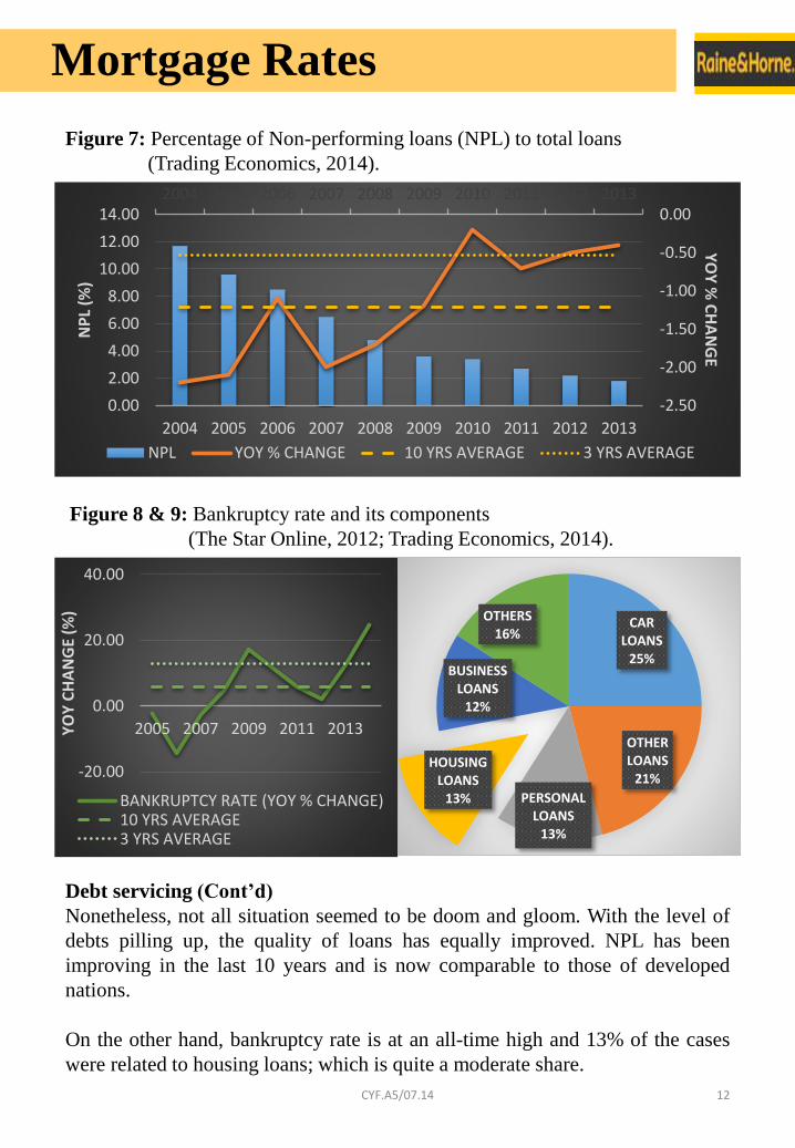
Figure 14: KLSE Property Index (CNBC, 2014).
10 years 5 years
1 year YTD
Another way of gauging the health of the property market is through
performance of the equities market. In this instance, the KLSE property index
which comprised of all builders and developers listed on the local bourse; were
analyzed to determine the health of the property market. Four different
timeframes were used, which consist of 10 years (long-term), 5 years (mid-
term), 1 year (short-term), and year-to-date (YTD: near-term).
It was noticed in all instances that the property market was and still is on an
uptrend; with higher support and higher resistance levels. Trading volumes were
strong and supportive of any surge. Thus, developers were still speculated to
perform well over the short and long-term.CYF.A5/07.14
Demographic Factors
19
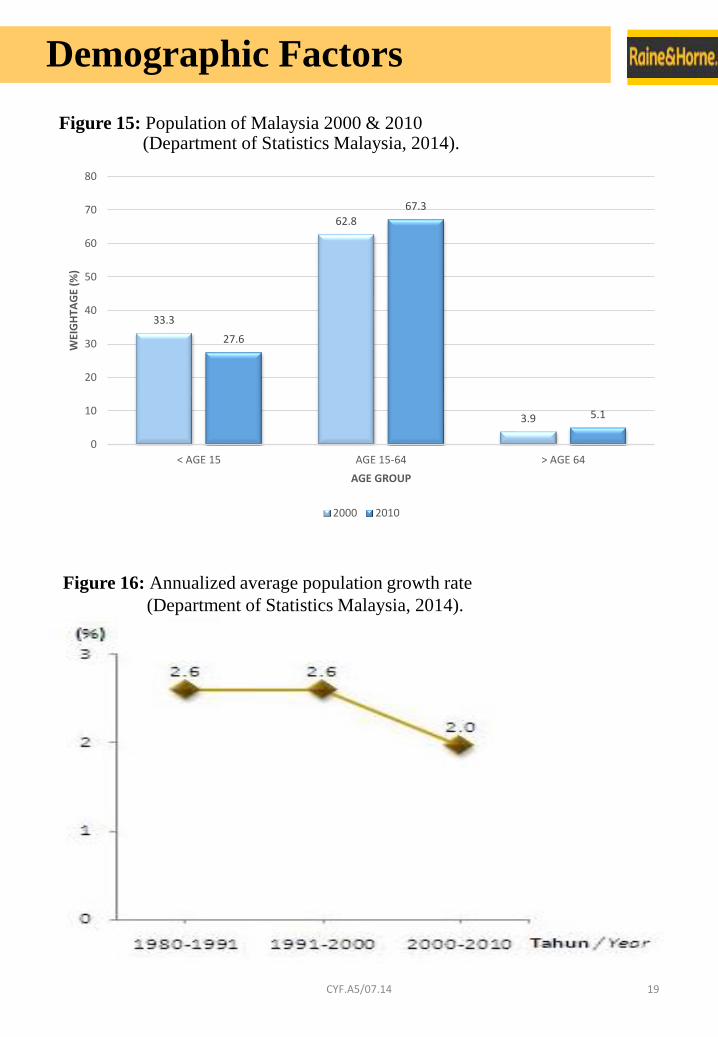
Figure 15: Population of Malaysia 2000 & 2010 (Department of Statistics Malaysia, 2014).
33.3
62.8
3.9
27.6
67.3
5.1
0
10
20
30
40
50
60
70
80
< AGE 15 AGE 15-64 > AGE 64
WEI
GH
TAG
E (%
)
AGE GROUP
2000 2010
Figure 16: Annualized average population growth rate
(Department of Statistics Malaysia, 2014).
CYF.A5/07.14

Demographic Factors
20
Population Growth Rate
Malaysia’s population is aging slowly (early stages); with lower portion of
children age group (< age 15) in 2010 compared to 2000. Working age adults
and retirement segments have increased by 4.5% and 1.2% respectively. Median
age has increased from 23.6 (2000) to 26.2 (2010); which is still a relatively
young population. Annualized average growth rate was stable at 2.6% from
1980 to 2000. A decline was observed from the subsequent period (2000 to
2010); to 2.0%.
The country’s dependency ratio has dropped from 0.59 (2000) to 0.49 (2010),
reinforcing the fact that:
1. population growth is slowing
2. children age group is diminishing (entering the age of workforce)
3. working age group is increasing
4. more working adults are supporting the non-working classes (children and
elders).
Refined grouping
Classification of the population in Malaysia was further refined to selective age
groups; to provide a better appraisal of the domestic workforce.
37.53
54.61
7.86
< AGE 20 AGE 20-59 > AGE 59
WEI
GH
TAG
E (%
)
AGE GROUP
2010
Figure 17: Refined population grouping 2010
(Department of Statistics Malaysia, 2014).
CYF.A5/07.14

Demographic Factors
21
Figure 18: Demographics by age group 2010
(Department of Statistics Malaysia, 2014).
0
2,000,000
4,000,000
6,000,000
8,000,000
10,000,000
12,000,000
0-19 20-29 30-39 40-49 50-59 60-75+
PO
PU
LATI
ON
AGE GROUP
POPULATION COUNT
KELANTAN, 1.16
TERENGGANU, 1.07
PERLIS, 1.01
KEDAH, 0.96
PAHANG, 0.96
SABAH, 0.93
PERAK, 0.93
SARAWAK, 0.91
MELAKA, 0.90
NEGERI SEMBILAN, 0.84
MALAYSIA, 0.83
JOHOR, 0.78
LABUAN, 0.74
PULAU PINANG, 0.73
SELANGOR, 0.65
KUALA LUMPUR, 0.62
PUTRAJAYA, 0.59
0.00 0.20 0.40 0.60 0.80 1.00 1.20 1.40
Figure 19: Dependency ratio by state 2010 (using refined grouping)
(Department of Statistics Malaysia, 2014).
CYF.A5/07.14

Demographic Factors
22
Refined grouping (Cont’d)
The refined grouping has increased the interval range for both children
(< 20 age) and retirees (> 59 age) by 5 years each. Hence, the number and range
of working adults (20 – 59 age) decreased by 10 years in total. As depicted in
Figure 17, the share of working adults was reduced to 54.6% of the total
population from the previous unrefined reading of 67.3%.
Further dissection of the working age group has reinforced the point that the
Malaysian workforce is indeed very young; with the highest percentage in the
20 – 29 age group, followed by 30 – 39. These 2 groups are ages of greatest
household formations.
Such refined grouping has increased the country’s dependency ratio to 0.83
from the initial calculation of 0.49. According to Figure 19, it was noted that a
total of 6 states in the country had better dependency ratio compared to the
national average. As expected, they include the more developed states; led by
Putrajaya (0.59), Kuala Lumpur (0.62), Selangor (0.65), Pulau Pinang (0.73),
Labuan (0.74), and Johor (0.78). Almost all of these states had received the
deserving attention from developers and buyers alike.
Whereas those with dependency ratio slightly below the national reading such
as Negeri Sembilan (0.84) and Melaka (0.90); was starting to command interest
from developers due to overcrowding of the respective markets as stated above.
CYF.A5/07.14

Demographic Factors
23
Figure 20: Distribution of Malaysian population by state 2010.
Figure 21: Urbanization rate by state 2010
(Department of Statistics Malaysia, 2014).
SELANGOR21%
SABAH12%
JOHOR9%
SARAWAK9%
PERAK7%
KEDAH7%
KUALA LUMPUR6%
PULAU PINANG6%
PAHANG5%
KELANTAN5%
TERENGGANU4%
NEGERI SEMBILAN3%
MELAKA3%
PERLIS1%
LABUAN0%
PUTRAJAYA0%
KELANTAN, 42.4
PAHANG, 50.5
PERLIS, 51.4
SARAWAK, 53.8
SABAH, 54.0
TERENGGANU, 59.1
KEDAH, 64.6
NEGERI SEMBILAN, 66.5
PERAK, 69.7
MALAYSIA, 71.0
JOHOR, 71.9
LABUAN, 82.3
MELAKA, 86.5
PULAU PINANG, 90.8
SELANGOR, 91.4
KUALA LUMPUR, 100.0
PUTRAJAYA, 100.0
0.0 20.0 40.0 60.0 80.0 100.0 120.0
CYF.A5/07.14

Demographic Factors
24
Figure 22: Population density (person/km2) 2010
(Department of Statistics Malaysia, 2014).
Figure 23: Household size 2010 (Department of Statistics Malaysia, 2014).
SARAWAK, 19
PAHANG, 40
SABAH, 42
TERENGGANU, 78
MALAYSIA, 86
KELANTAN, 97
PERAK, 110
NEGERI SEMBILAN, 150
JOHOR, 174
KEDAH, 199
PERLIS, 280
MELAKA, 470
SELANGOR, 674
LABUAN, 950
PUTRAJAYA, 1,478
PULAU PINANG, 1,500
KUALA LUMPUR, 6,891
0 1,000 2,000 3,000 4,000 5,000 6,000 7,000 8,000
SABAH, 5.88
KELANTAN, 4.86
TERENGGANU, 4.78
LABUAN, 4.72
PAHANG, 4.59
SARAWAK, 4.47
MALAYSIA, 4.31
KEDAH, 4.29
PERLIS, 4.26
NEGERI SEMBILAN, 4.20
JOHOR, 4.17
MELAKA, 4.05
PERAK, 4.04
PULAU PINANG, 3.94
SELANGOR, 3.93
KUALA LUMPUR, 3.72
PUTRAJAYA, 3.45
0.00 1.00 2.00 3.00 4.00 5.00 6.00 7.00
CYF.A5/07.14
Demographic Factors
25
Distribution
The top 5 states in Malaysia in regards to number of inhabitants were Selangor
(21%), Sabah (12%), Johor (9%), Sarawak (9%), and Perak (7%). Some of the
reasons as to why Sabah, Sarawak, and Perak were less favored by developers
include the vast land size compared to the number of population; resulting in
low population density, relatively poor infrastructures, low rate of urbanization,
and unfavorable dependency ratio.
Urbanization
Malaysia recorded a fairly moderate urbanization rate of 71.0% in 2010.
Mimicking the chart of dependency ratio; with both the Federal Territories in
Peninsular Malaysia posted 100.0% urbanization rate. Other usual members
above the national average were Selangor (91.4%), Pulau Pinang (90.8%),
Labuan (82.3%) , and Johor (71.9%). The only surprise was Melaka which
came in 86.5%.
Density
Malaysia has a low population density ratio coming in at just 86 person/km2.
This suggests that the nation’s population is not evenly distributed with
concentrations in a few selective states. The most dense state is Kuala Lumpur
(6,891 person/km2: comparable to Singapore and Hong Kong), followed by
Pulau Pinang (1,500 person/km2), Putrajaya (1,478 person/km2), Labuan
(950 person/km2), Selangor (674 person/km2), and Melaka (470 person/km2).
The degree of density usually dictates the type of houses offered by developers.
Household Size
Malaysia has a fairly large household size of 4.31 person/household. It is
anticipated that there could be a high possibility of smaller household size in the
future. Such a reduction in the number of person per household would directly
increase the demand for new living quarters and strain the existing housing
stock in the market. In addition, smaller household size would translate into
demand for smaller residential units as well.
CYF.A5/07.14

Micro Factors
26
As revealed earlier, macro drivers affect the property market at a national scale,
while micro drivers emphasize on local conditions of the subject property. The
main equation of hedonic regression by Wheatley (2012) are as follow:
P = f (L, T, S, V, N)
P: price of house
f: function of
L: location characteristics
T: house characteristics
S: plot size
V: surrounding view
N: neighbourhood characteristics
The above equation proposed that the price of house is a function of several
local variables such as location characteristics, house characteristics, plot size,
surrounding view and neighbourhood characteristics. These factors usually
adhere to a general guideline but in some instances, may subject to personal
preference.
In common, a house could usually command a higher price by locating in close
proximity to commercial and recreational areas, possessing superior building
quality and design, built on a larger land size, surrounded by ideal view such as
lush sceneries or unobstructed view of the city, and enclosed in a clean and safe
neighbourhood.
Buyers would be more willing to pay a higher price for the house if these
related characteristics matched their individual expectations and preferences.
CYF.A5/07.14
References
Bank Negara Malaysia (BNM). (2014) Rates & Statistics, Kuala Lumpur: BNM
Publications, [Online], Available:
http://www.bnm.gov.my/index.php?ch=statistic&lang=en [18 Jun 2014].
CNBC. (2014) KLSE Property Index, [Online], Available:
http://data.cnbc.com/quotes/PROPERTIES/tab/2 [1 July 2014].
Department of Statistics Malaysia. (2014) Gross domestic product at current
prices, [Online], Available:
http://www.statistics.gov.my/portal/index.php?option=com_content&view=artic
le&id=2261 [18 Jun 2014].
Department of Statistics Malaysia. (2014) Statistical Releases, [Online],
Available: http://www.statistics.gov.my/portal/index.php?option=
com_content&view=article&id=472&Itemid=111&lang=en&negeri=Malaysia
[15 Jun 2014].
EPF. (2014) Dividend Rates, [Online], Available:
http://www.kwsp.gov.my/portal/about-epf/investment-highlights/dividend-
rates/dividend-rates [18 Jun 2014].
Freddie Mac. (2014) 30-Year Fixed-Rate Mortgages, [Online], Available:
http://www.freddiemac.com/pmms/pmms30.htm [18 Jun 2014].
JPPH. (2014) Property Market Report 2013, Putrajaya: Valuation and Property
Services Department.
Kaplan University. (2013) Schwesernotestm 2014 CFA Level I Book 2:
Economics, United States of America: Kaplan Inc.
NAPIC. (2014) Key Statistics, [Online], Available:
http://napic.jpph.gov.my/portal [15 Jun 2014].
The Star Online. (2012). ‘A second chance for bankrupts’, The Star Online, 9
December, [Online], Available:
http://www.thestar.com.my/story.aspx/?file=%2f2012%2f12%2f9%2fnation%2f
12434811&sec=nation [18 Jun 2014].
27CYF.A5/07.14

References
The Star Online. (2014). ‘Malaysia's rising household debt hits new record of
86.8% of GDP’, The Star Online, 20 March, [Online], Available:
http://www.thestar.com.my/business/business-news/2014/03/20/rising-
household-debt-it-hits-new-record-of-868-of-gdp-on-loans-for-properties-and-
motor-vehicles/ [18 Jun 2014].
Trading Economics. (2014) Malaysia Economic Indicators, [Online], Available:
http://www.tradingeconomics.com/malaysia/indicators [18 Jun 2014].
Wheatley D. (2012) Hedonic Pricing Method, [Online], Available:
http://www.cbabuilder.co.uk/Quant5.html [18 Jun 2014].
28CYF.A5/07.14

Contact us
29
OFFICE EMAIL TELEPHONE
HQ (KL) [email protected] 603 26980911
Petaling Jaya [email protected] 603 78806542
Subang Jaya [email protected] 603 56319668
Klang [email protected] 603 33420193603 33420182
Ipoh [email protected] 605 2532804605 2413888
Seremban [email protected] 606 6333211
Melaka [email protected] 606 2860017606 2840017
Penang [email protected] 604 2638093604 2612032
Johor Bahru [email protected] 607 3863791607 3863795
Kuantan [email protected] 609 5157100
Kuching [email protected] 6082 235236
Kota Kinabalu [email protected] 6088 266520
CYF.A5/07.14

International Affiliations
30
Country Affiliates
Australia
Corporate Office – SydneyNew South Wales – Sydney
Queensland –BrisbaneVictoria - Melbourne
South Australia – Kent TownTasmania – Hobart
Western Australia – South PerthNorthern Territory – Parap
Austria DMH Vienna
Belgium Activia Belgium SA
Czech Republic Huber Holdings Prag s.r.o
Fiji Raine & Horne Fiji
Hong Kong Raine & Horne Projects Hong Kong
Hungary Dr. Max Huber Kft.
India Arora & Associates Realty Ltd.
Italy GC International S.R.L.
JapanKiuchi Property Counselors & Valuers
Inc
United Kingdom Raine & Horne Crossgates
UAE Raine & Horne Dubai
Vanuatu Raine & Horne Vanuatu
CYF.A5/07.14

Raine & Horne International Zaki + Partnerswww.raineandhorne.com.my
Perpetual 99, Jalan Raja Muda Abdul Aziz, 50300 Kuala Lumpur
Tel: 03-2698 0911 Fax: 03-2691 1959 Email: [email protected]
Company No. 99440-T, VE (1) 0067
31