Drivers of Regional Efficiency Differentials in Italy: Technical Inefficiency or Allocative Distortions?

Drivers of Regional Efficiency Differentialsin Italy: Technical Inefficiency or

Allocative Distortions?

FABRIZIO ERBETTA AND CARMELO PETRAGLIA

ABSTRACT This paper estimates regional economic efficiency differentials at the firm level

for the Italian manufacturing sector in the period 1998–2003. We implement an input distance-

function approach providing measures of both technical inefficiency and allocative distortions in

the choice of input mixes. Our results confirm the substantial technical efficiency gap suffered by

firms located in Southern regions, thus providing empirical support for the “structural and tech-

nological gap” interpretation of Italian dualism. On the other hand, the allocative distortions in the

use of inputs show less-remarkable regional differences. In terms of policy, our results suggest the

need for a reallocation of public resources for development policies from business incentives to

public investment.

Introduction

T he dualistic structure of the Italian economy—the so-called “Mezzogiorno”1

and the rest of the country—is probably unique among the countries of theEuropean Union. Public intervention for the economic and social development ofSouthern Italian regions dates back to the 1950s, since when there has beenimplementation of both demand- and supply-oriented policies.2 However, theItalian Mezzogiorno still lags behind the rest of Italy.

It has been acknowledged that demand-linked regional policies since the 1980shave not produced positive results, and supply-side-based interpretations of Italy’s

Fabrizio Erbetta is an assistant professor in the Department of Management and Territorial

Studies, The University of Eastern Piedmont, Via Perrone 18, Novara, I-28100, Italy. He is a research

associate at the Ceris-CNR (Institute for Economic Research on Firms and Growth) and HERMES

(Higher Education and Research on Mobility Regulation and the Economics of local services), Via

Real Collegio 30, Moncalieri (TO), I-10024. His e-mail address is: [email protected].

Carmelo Petraglia (corresponding author) is an assistant professor in the Department of Economics,

The University of Naples “Federico II,” Complesso Universitario di Monte Sant’Angelo, Via Cinthia,

80126, Naples, Italy. His e-mail address is: [email protected]. We thank Graziano Abrate,

Ciro Avitabile, Matteo Ferraris, Giovanni Fraquelli, and Adriano Giannola for useful discussion. We

are indebted with three anonymous referees whose comments significantly helped to improve the paper.

Usual disclaimers apply.

Growth and ChangeVol. 42 No. 3 (September 2011), pp. 351–375

Submitted July 2010; revised February 2011; accepted March 2011.© 2011 Wiley Periodicals, Inc

dualism have gained credibility and promoted public policies in the shape of bothincentives to private capital accumulation and public investment. The emphasisput on either incentives to private investment or public investment policies crudelyreflects the two alternative supply-side explanations for Italy’s dual economicstructure, i.e., it reflects the “market-oriented” and the “structural and technologi-cal gap” views (Destefanis 2001).

According to the market-oriented view, market failures in the efficient alloca-tion of resources are more severe in the Mezzogiorno than in the Northern Italianregions. In this view, allocative inefficiency is regarded as the main source ofperformance differentials between Southern and Northern firms. Hence, firmsneed well-designed incentives in order for local resources to be employed mosteffectively and efficiently, in the presence of soft “external” public intervention.On the other hand, those scholars who adhere to the view of a structural andtechnological gap emphasise the role played by the structural poverty of theMezzogiorno economy producing a less-favourable environment (e.g., transportand communications, education, and public order), which considerably reducesthe technological possibilities of local firms. Indeed, given the uncertainty of theeconomic system, many Southern entrepreneurs may be reluctant to undertakeinvestment programmes aimed at improving technology and at enhancing theiroperating scale. At the same time, there are few incentives for workers to improvetheir skills or to benefit from learning opportunities (Cenci and Scarlato 2002).The combined effect of these factors is likely to hamper technical efficiency.Hence, public investment is crucial for improving environmental conditions andreducing uncertainty.

Because of the complexity of the problem in terms of both the number ofvariables involved in the analysis and its historical persistence, it would be mis-leading to lean toward one or other of the explanations referred to above. However,in terms of the implications for policy, it is clear that empirical support for theseviews would help in the design and implementation of effective policies thatwould enhance productivity in the Mezzogiorno economy.

With this in mind, we evaluate the productivity gap between Southern firms andthose located in the rest of the country by estimating sector-specific input distancefunctions. This approach will allow us to distinguish regional differentials relatedto technical inefficiency, from those due to allocative distortions in the choice ofinput mixes. We interpret the presence of the former as supporting the structuraland technological gap view and the latter as supporting the market-oriented view.

The paper is structured as follows: The second section briefly reviews thealternative supply-side views of Italian dualism and introduces the main featuresof recent development policies for the Italian Mezzogiorno. The third section

352 GROWTH AND CHANGE, SEPTEMBER 2011

discusses methodological aspects of the input distance function, and the fourthsection presents the data set and the model. The empirical specification is providedin the fifth section, and the sixth section summarises the results. The mainconclusions are presented in the last section of the paper.

Regional Development Policies and Supply-side Interpretations ofItalian Dualism

Development policies for the Italian Mezzogiorno. During the 1980s, Italianregional policies were based on measures aimed at stimulating the demand side ofthe economy by means of fiscal subsidies to firms and income support for house-holds and job creation measures in the public sector. These policies were based onthe idea of “endogenous” development: Supporting local demand was expected tocreate local supply and boost local industrial activities. This strategy failed,however, because of the strong economic dependence of the Mezzogiorno onNorthern regions. Supporting local demand, far from stimulating local supply, ledto increased imports from the North, which crowded out local industrial activities(Del Monte and Giannola 1997). Following this policy failure, supply-side inter-pretations of Italian dualism gained credibility in the late 1990s, promoting aswitch to policies based on both incentives for private investment and productivepublic expenditure.

Since the late 1990s, a new strategy of public intervention has been adopted inan attempt to reconcile policy-making confidence in the capabilities of less-developed areas to attain endogenous development, with calls for extensive“external” intervention aimed at improving the local, social, and economiccontext. The declared ultimate aim of this strategy was the creation of the condi-tions required for a self-sustaining development process through improvements tothe socio-economic and institutional context of the area. A distinguishing featureof this new policy of public intervention is a “bottom-up” strategy in which bothplanning and implementation processes are extensively decentralised to regionaladministrations.3

Development policies are designed to improve market competition for labour,goods, and financial capital; communications; training of human resources andinnovation opportunities; social infrastructures; internal relations; externalitiesfrom agglomerations of entrepreneurial activities; and accessibility to natural andcultural resources (Barca 2003, 2006). The main instruments employed to achievethese ambitious goals fall into two categories: incentives for private investmentand the provision of public goods via public investment. From a policy-makingpoint of view, support for business should be temporary and should foster capitalaccumulation (and thus local employment and income) in less-developed areas to

REGIONAL EFFICIENCY DIFFERENTIALS IN ITALY 353

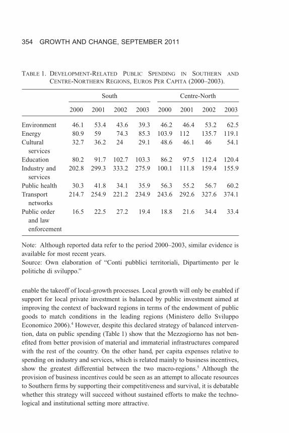
enable the takeoff of local-growth processes. Local growth will only be enabled ifsupport for local private investment is balanced by public investment aimed atimproving the context of backward regions in terms of the endowment of publicgoods to match conditions in the leading regions (Ministero dello SviluppoEconomico 2006).4 However, despite this declared strategy of balanced interven-tion, data on public spending (Table 1) show that the Mezzogiorno has not ben-efited from better provision of material and immaterial infrastructures comparedwith the rest of the country. On the other hand, per capita expenses relative tospending on industry and services, which is related mainly to business incentives,show the greatest differential between the two macro-regions.5 Although theprovision of business incentives could be seen as an attempt to allocate resourcesto Southern firms by supporting their competitiveness and survival, it is debatablewhether this strategy will succeed without sustained efforts to make the techno-logical and institutional setting more attractive.

TABLE 1. DEVELOPMENT-RELATED PUBLIC SPENDING IN SOUTHERN AND

CENTRE-NORTHERN REGIONS, EUROS PER CAPITA (2000–2003).

South Centre-North

2000 2001 2002 2003 2000 2001 2002 2003

Environment 46.1 53.4 43.6 39.3 46.2 46.4 53.2 62.5Energy 80.9 59 74.3 85.3 103.9 112 135.7 119.1Cultural

services32.7 36.2 24 29.1 48.6 46.1 46 54.1

Education 80.2 91.7 102.7 103.3 86.2 97.5 112.4 120.4Industry and

services202.8 299.3 333.2 275.9 100.1 111.8 159.4 155.9

Public health 30.3 41.8 34.1 35.9 56.3 55.2 56.7 60.2Transport

networks214.7 254.9 221.2 234.9 243.6 292.6 327.6 374.1

Public orderand lawenforcement

16.5 22.5 27.2 19.4 18.8 21.6 34.4 33.4

Note: Although reported data refer to the period 2000–2003, similar evidence isavailable for most recent years.Source: Own elaboration of “Conti pubblici territoriali, Dipartimento per lepolitiche di sviluppo.”


Supply-side interpretations of the Italian dualism. As already argued, pri-oritising either well-designed incentives or public-investment policies reflects thetwo different supply-side interpretations of Italian dualism: the market-orientedand the structural and technological gap views. The key point for market-orientedscholars is the higher extent to which Southern firms fail to allocate availableproductive resources efficiently. There are many examples of this. Asymmetricinformation between the two sides of the labour market due to uncertainty aboutthe workers’ real skills on the one hand, and the opportunities for career advance-ment offered by the firms on the other, results in a mismatch between the twogroups of agents in this market and leads to inefficient allocation of the workforce(Cenci and Scarlato 2002). In addition, credit market imperfections can lead toincorrect evaluation of investment projects, resulting either in under-investment orin firms being forced to use their own resources to finance investment. Hence,performance differences across Italian regions are mainly seen as stemming fromhigher input allocative inefficiency in the South and, in this view, well-designedincentives for firms should produce an efficient exploitation of resources.

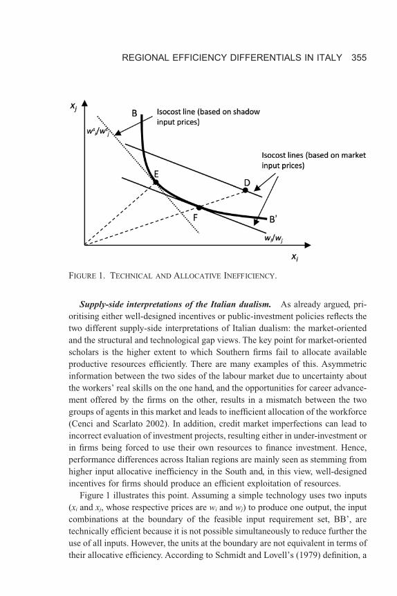
Figure 1 illustrates this point. Assuming a simple technology uses two inputs(xi and xj, whose respective prices are wi and wj) to produce one output, the inputcombinations at the boundary of the feasible input requirement set, BB’, aretechnically efficient because it is not possible simultaneously to reduce further theuse of all inputs. However, the units at the boundary are not equivalent in terms oftheir allocative efficiency. According to Schmidt and Lovell’s (1979) definition, a

FIGURE 1. TECHNICAL AND ALLOCATIVE INEFFICIENCY.


producer is allocatively efficient if it succeeds in allocating inputs in such a waythat the marginal rate of technical substitution equates the input price ratio. InFigure 1, while the input combination of unit F ensures cost minimisation, unit E,although technically efficient, does not, as it shows excessive use of input j withrespect to input i, given the market input prices. This distortion in input demandlevels disappears at the input shadow price ratio ws

i/wsj. This means that, for firm

managers deciding about input demand, the relevant relative prices diverge tosome extent from actual (market) prices. This divergence may be due to a numberof environmental factors that make the objective of cost minimisation unafford-able. The divergence between the shadow price ratio and the market price ratioprovides a direct measure of the allocative distortion embedded in a given inputmix.6 When the allocative distortion is such that some inputs are systematicallyfavoured over others, there is a need for proper business incentives aimed atstimulating adjustments to the input demand decisions that are consistent with themarket price set.

Adherents to the structural and technological gap view (e.g., Costabile 1996)emphasise the role played by the structural poverty of the Mezzogiorno economyin terms of its less-favourable environmental conditions. According to this view,technical efficiency can be regarded as the main source of regional differences inperformance. As Figure 1 shows, the input mix of unit D is allocatively efficient,but the input levels are technically inefficient. Therefore, public policies should beaddressed mainly to removing, or at least mitigating, those factors that system-atically foster the overuse of inputs. In this case, an integrated system of publicinterventions (including, e.g., improved communication and transportation infra-structures, establishment of high-quality education systems, and enforcement ofpublic order) may be regarded as more suited to creating the conditions for privateinvestment in less-developed areas to be more productive.

Modelling Technical Inefficiencies and Allocative DistortionsEconomic efficiency involves technical and allocative components (Farrell

1957). In general terms, technical efficiency reflects the manager’s capacity tominimise input utilisation and to reduce waste, while the concept of allocativeefficiency is based on the ability to define a cost-minimising input mix, givenmarket factor prices. The approach used to derive estimates of technical efficiencyand allocative distortions is the input distance function. Furthermore, becausetechnology can differ greatly among industries, we compute separate efficiencymeasures for the different industries.7

The input distance function has several advantages over the traditional costfunction model (see, among others, Coelli and Perelman 2000; Färe and


Grosskopf 1990; Färe and Primont 1995; Grosskopf et al. 2001).8 First, estimationof a cost function assumes that all firms are equally able to express input require-ments consistent with cost minimisation. Cost-frontier models allow the removalof this restrictive assumption, although still within a cost-minimising framework.In these models, the cost of inefficient units differs from the minimum attainablecost based on an inefficiency term that combines technical and allocative com-ponents, and pure random noise. Unfortunately, this approach makes the separa-tion of technical and allocative inefficiency terms problematic and subject toundesirable restrictions. In contrast to cost functions, input distance functions arerobust to deviations from the neoclassical cost-minimising paradigm. The dualitybetween the input distance function and the shadow cost function makes theformer free from cost-minimising assumptions because it is based on the assump-tion that input levels are selected according to shadow (implicit) rather than tomarket input prices, as is often the case for regulated or publicly owned firms,or when bureaucratic behaviour—based on principal-agent informationasymmetries—imposes private utility maximisation (Färe and Primont 1995).Similarly, this behaviour-free characteristic makes the input distance functionsuitable for any situation where exogenous market forces might fail to organiseavailable resources in an economically convenient way so that public interventionis needed to promote input adjustments. Indeed, the duality properties can be usedto identify the intrinsic shadow price ratio and, therefore, to infer evidence aboutinput misallocation. Finally, estimation of the input distance function does notrequire direct information about market input prices, information that often isdifficult to obtain in a truly exogenous way.

Formally, the input distance function (DI) is defined as follows:

D y x x L yI ( , ) max{ : / ( )}= ∈δ δ (1)

where x and y denote, respectively, a (N ¥ 1) input vector and a (M ¥ 1) outputvector, and L(y) is the production possibility set including all the feasible inputcombinations that can produce a given output level y. For x ∈ L(y) the distanceparameter d, which represents a natural measure of technical efficiency, is �1,being equal to 1 if and only if x is technically efficient.9 Therefore, the greaterDI(y, x), the lower the technical efficiency associated with each producer.

The distance function must satisfy some regularity conditions (Färe andPrimont 1995): It must be non-decreasing, linearly homogeneous, and concave inthe input vector x and non-increasing in the output vector y.

The duality relationship between the input distance function and the shadowcost function is defined by the following equations:


C y w w x D y xsx

sI( , ) min { : ( , ) }= ≥1 (2)

D y x W x C y WI Ws s

s( , ) min { : ( , ) }= ≥1 (3)

where C(y, w s) is the shadow cost of producing the output vector y, given the inputshadow price vector ws, and Ws = ws/C(y, ws) is a vector of the cost-deflated inputshadow prices. Because the cost function is homogeneous to degree 1 in inputprices, the resulting value of C(y, W s) will be greater than or equal to 1. Shadowprices, ws, represent the implicit (unobserved) input prices that support the man-ager’s optimal input demand, given the output level to be produced. If the relativeinput shadow prices differ from the relative input market prices, an allocativedistortion problem will arise, meaning that input demand will deviate from itscost-minimising level.

Following Färe and Grosskopf (1990), in a shadow price model, such as the onedefined in equations (2) and (3), where firms are assumed to minimise the shadowcost, the application of the dual Shephard’s (1953) lemma yields the followingexpression of the first partial derivative of the input distance function with respectto input quantity xi:

∂∂

= =D y x

xW y x

w

C y wI

iis i

s

s

( , )( , )

( , )(4)

for i = 1, . . . , N.Because the shadow cost function C(y, w s) is not observable, the input shadow

prices, wis, cannot be calculated directly. However, the ratio between the two first

partial derivatives of the input distance function with respect to inputs i and jyields the shadow price ratio (Grosskopf et al. 2001; Rodríguez-Álvarez,Fernández-Blanco, and Lovell 2004):

∂ ∂∂ ∂

=D y x x

D y x x

w

wI i

I j

is

js

( , )

( , )(5)

for i, j = 1, . . . , N and i � j.This ratio can be used to evaluate the existence of input misallocation. Indeed,

a measure of input allocative distortion can be obtained by comparing the shadowprice ratio with the market price ratio (or, in other words, by comparing the slopesof the two isocost lines depicted in Figure 1) as follows:

w w

w wki

sjs

i jij= (6)


If kij = 1 (i.e., wis/wi = wj

s/wj), the input mix is allocatively efficient; if kij > 1 (i.e.,wi

s/wi > wjs/wj), firms under-utilise input i relative to input j, and if kij < 1 (i.e.,

wis/wi < wj

s/wj), firms over-utilise input i relative to input j. In the latter two cases,the non-optimal input mix deviates from the cost-minimising one, as the pricesthat support the input demand differ from market prices.

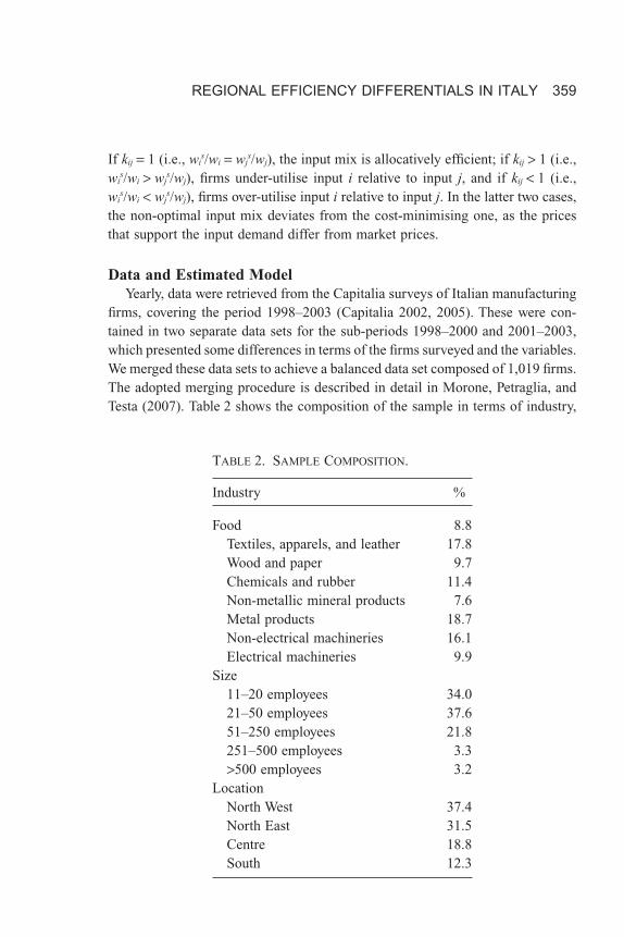
Data and Estimated ModelYearly, data were retrieved from the Capitalia surveys of Italian manufacturing

firms, covering the period 1998–2003 (Capitalia 2002, 2005). These were con-tained in two separate data sets for the sub-periods 1998–2000 and 2001–2003,which presented some differences in terms of the firms surveyed and the variables.We merged these data sets to achieve a balanced data set composed of 1,019 firms.The adopted merging procedure is described in detail in Morone, Petraglia, andTesta (2007). Table 2 shows the composition of the sample in terms of industry,

TABLE 2. SAMPLE COMPOSITION.

Industry %

Food 8.8Textiles, apparels, and leather 17.8Wood and paper 9.7Chemicals and rubber 11.4Non-metallic mineral products 7.6Metal products 18.7Non-electrical machineries 16.1Electrical machineries 9.9

Size11–20 employees 34.021–50 employees 37.651–250 employees 21.8251–500 employees 3.3>500 employees 3.2

LocationNorth West 37.4North East 31.5Centre 18.8South 12.3


size, and geographical location. Consistent with the features distinctive of theItalian economic system, which is characterised by a prevalence of small andmedium enterprises, more than 70 percent of the sample firms employ less than 50people, and more than two-thirds are located in the more developed Northernregions.

The stochastic input distance-function system assumes the following form:

ln( ) ln ( , )1 = +D y x vI (7)

w x

C

D y x

xvi i I

ii= ∂

∂+ln ( , )

ln( )(8)

for i = 1, . . . , N and where C is the actual cost and v and vi are the statistical noiseterms, assumed to have a normal distribution with zero mean and constant vari-ance. Equation (7) represents the input distance function in log form. Because thevalue of the input distance function is equal to 1 at the frontier, the log specifi-cation implies that a firm is technically inefficient if lnDI(y, x) is greater than zero.Equation (8) represents the cost share for input i derived using the dual Shep-hard’s lemma defined in equation (4).

To explain formally the derivation of the market price ratio correction index, kij,from the input distance-function model (7)–(8), we express the dual Shephard’slemma in log form as follows:

∂∂

=ln ( , )

ln( ) ( , ) ( , )

D y x

x

w

C y w

x

D y xI

i

is

s

i

I

(9)

Then, from equation (9) and given that for the actual input combination, theshadow cost is equal to the actual cost evaluated at the frontier(Rodríguez-Álvarez and Lovell 2004), i.e., C(y, ws) = C/DI(y, x), we obtain

∂∂

=ln ( , )

ln( )

D y x

x

w x

CI

i

is

i(10)

which represents the optimal input share equation with respect to the shadowprices. Deviation from this optimal share is attributable to allocative inefficiencyand noise, both encompassed by the unique disturbance term, vi.

The index of allocative distortion kij defined in equation (6) is computed foreach observation using the following expression:

∂∂

∂∂

= ⎛

⎝⎜

⎞

⎠⎟

ln ( , )

ln

ln ( , )

ln

D y x

x

D y x

xk

w x C

w x CI

i

I

jij

i i

j j

(11)


Given that the first partial derivative of the log-distance function with respect tothe log of input i represents the i-th input optimal cost share, the kij coefficient maybe seen as the ratio of the optimal input cost shares compared with the ratio of theactual input cost shares.

The estimated kij represent relative measures of distortion in the use of oneinput with respect to another. However, they do not provide direct information onthe excess cost due to input misallocation. To determine the overall cost ofallocative inefficiency, we follow the three-step procedure proposed byRodríguez-Álvarez, Fernández-Blanco, and Lovell (2004). In the first step, assum-ing input-specific allocative distortion parameters zi, such that zixi = xi* representsthe cost-minimising input level, we obtain from equation (11)

∂∂

∂∂

=ln ( , )

ln

ln ( , )

ln* *

D y x

x

D y x

x

w z x

w z xI

i

I

j

i i i

j j j(12)

from which we have that

∂∂

∂∂

=

ln ( , )

ln

ln ( , )

ln* *

D y x

x

D y x

x

w x w x

z

z

I

i

I

j

i i j j

i

j

(13)

This is a system of N-1 equations in N variables zi. However, because theshare equation is homogeneous of degree zero in inputs, it is possible tonormalise by some arbitrarily chosen cost-minimising input level. By lettingxN* be the chosen numeraire, we can reduce the system of equation (13) to asystem of N-1 non-linear equations in N-1 variables ziN (ziN = zi/zN) such thatxi* = ziNzNxi.

In the second step, from the calculated values ziN, it is possible to determine zN

by substituting the coefficients ziN into the estimated input distance function:

ln ( , ) ln( )D y z z xI iN N i = 1 (14)

which represents the transformation function at the technically efficient boundarylevel. Hence, the allocative distortion coefficients zi are simply derived aszi = ziNzN.

Finally, the cost of the allocative inefficiency index can be determined as10

1− ⎛⎝⎜

⎞⎠⎟∑w z x Ci i i

i(15)


Empirical SpecificationTo estimate the model, we used a translog input distance function defined as11

ln( ) ln ln ln

ln ln

11

21

2

2= + + ( ) +

+

∑

∑∑

y x y

x x

y ii

imt yy

ij imt jmtji

β β β

β ++

+ + + +

∑

∑ ∑

β

δ δ η

yi imti

tt

t tSOUTH t SOUTHt

m mt

y x

D D D v

ln ln (16)

The cost share equations are

w x

Cx y vimt imt

i ij jmtj

yi imt= + + +∑β β βln ln (17)

for i, j = 1, . . . , N inputs and where C represents total cost.The subscripts m and t denote firm and year, respectively; y refers to total

operating revenues; xi refers to inputs, including labour (number of employees, l),operating costs of the materials and services provided by other firms (cms) andcapital (tangible and intangible net fixed assets, k);12 Dt is a set of time dummies;DSOUTH is a geographical dummy that assumes the value 1 if the firm is located inSouthern Italy and 0 otherwise. Restrictions for homogeneity of degree 1 in inputs( β β βi

iyi

iij

i

j∑ ∑ ∑= = = ∀1 0 0; ; ) and symmetry (bij = bij "i � j) are

imposed in the estimation.13

We assume that the error term in equation (16) has the structure hm + vmt wherehm reflects firm-specific disturbances that capture all-time invariant componentsnot explicitly accounted for in the model and vmt ~ N(0, σ v

2) is a traditional randomnoise assumed to be uncorrelated with the hm term and regressors.

Because the amount of inputs may depend on criteria other than cost minimi-sation and the underlying incentives for choosing inputs might be linked tofirm-specific omitted characteristics, the hm error term cannot reasonably beassumed to be uncorrelated to the input regressors. One way to allow for corre-lation without incurring estimation bias is to treat the time-invariant individualcomponents as fixed effects and include a set of firm-specific dummy variables inthe input distance function equation, which traditionally are interpreted as tech-nical inefficiency indices at firm level.14

An important implication of the model specified above is that it is impossibleto control for any other time-invariant component such as geographical charac-teristics. To account for regional-level heterogeneity, we specify a set of timedummies that reflect the specific business cycle conditions to which firms are


exposed.15 In particular, the dt parameters capture the specific temporal effects ofCentre-North as the base case, while the dtSOUTH parameters allow us to test thedifference for the South against the benchmark. Thus, the inclusion of thesedummy variables allows us to control for time-varying regional differences.

Interpretation of the parameters associated with time and especially firm het-erogeneity deserves attention. Simplifying equation (16) in a convenient way, itfollows that the input distance-function equation can be written as

− ( ) = + + +∑ ∑ln ,D y x D D D vI t tt

tSOUTH t SOUTHt

m mtδ δ η (18)

where we can see that a negative sign of the parameters dt and dtSOUTH and anegative value of the estimated fixed effect hm entail an upward shift in thedistance function, indicating a worsening impact on efficiency of time, regionaland individual factors, respectively. The reverse is true in the case of positive signof the above parameters.

To clean the data set of potential outliers, we use the multivariate Hadi (1994)procedure with a 1 percent level of significance of outlier cut-off. All monetaryvariables are expressed in year 2000 Euros. For revenues, materials, and servicesby industry, we use the Istituto Nazionale di Statistica production price indices.16

Deflation of the capital variable proved more difficult because capital stock trendcan be affected by discontinuities due to monetary revaluation. To mitigate thiseffect, we adopt a perpetual inventory method. Starting from the more recent netfixed assets value (assumed to be the most accurate capital measure encompassingall past monetary adjustments), we reconstruct backwards the capital time seriesby subtracting yearly deflated net investments.

All input and output variables are divided by their respective geometric mean.This allows direct interpretation of the estimated coefficients of the first-orderterms as the elasticity of the distance function with respect to inputs and outputsat the sample mean. Also, according to Shephard’s lemma, the first-order inputcoefficients represent the optimal shares at the sample mean.

Finally, it is important to note that the input variables may be endogenous dueto the presence of omitted factors that affect the deviation of shadow from marketprices. Although the fixed effects specification may control partially for endoge-neity,17 we cannot exclude that further sources of endogeneity might remain due toomitted variables at group level not accounted for explicitly in the estimatedmodel. Therefore, as a robustness check, we estimate the equation system using theThree-stage least squares (3SLS) technique, instrumenting inputs variables andtheir interactions with their lagged values, output (first and second order terms),time dummies, and input prices (Atkinson, Cornwell, and Honerkamp 2003).


ResultsThe translog input distance function and the derived share equations are esti-

mated jointly by a seemingly unrelated regression estimation technique. Table 3shows the sector-by-sector results for the equation system (16)–(17).18 The esti-mated distance function appears to fit the observed data reasonably well. First-order terms represent the ideal input cost shares. They are always statisticallysignificant at the 1 percent level, have the expected sign, and are of plausiblemagnitude. The labour input cost share varies between 13 percent and 26 percent,the cost share of external supplies varies from 69 percent to 83 percent, and thecapital cost share varies between 4 percent and 7 percent (thus indicating anaverage recovery horizon of 15–25 years).

Second-order coefficients represent the (positive or negative) change in thedistance function elasticity with respect to input or output due to a 1 percentincrease in one technological variable. These parameters, in general, are statisti-cally significant and of reasonable magnitude.

In terms of temporal effects, the dt parameters are generally negative andstatistically significant, indicating that during the observed period, the businesscycle of Centre-North was predominantly declining. Also, the parameters dtSOUTH

show that in three industries, the South suffered from worse technical-changeconditions than the benchmark, and in only one case does it achieve a better result.The pattern for the other four sectors is more mixed. In almost all cases, however,the estimated coefficients indicate technical regress for the South.19

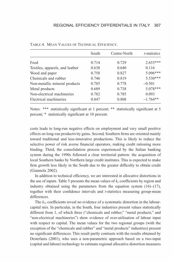
The technical efficiency score estimates, based on the time-invariant fixedeffects, are summarised in Table 4.20 With the notable exception of firms in the“electrical machineries” industry, the cross-regional comparison highlights a gen-erally lower efficiency of Southern firms of more than 7 percent. This result is inline with previous evidence (Destefanis 2001; Giannola and Petraglia 2006) basedon different frontier approaches and also seems to confirm the ex-ante assump-tions about the disadvantages suffered by Southern firms.21 Explanations for theseresults are various and range—as already noted—from poor infrastructuralendowment to a less-qualified workforce.

Also important is the role of credit market imperfections that have a heavyimpact on investment opportunities and growth (Sarno 2003). In terms of theirparticularities in the Mezzogiorno, several aspects are interesting. First, it hasbeen well documented that financial pressures are higher, ceteris paribus, forSouthern firms in terms of higher interest rates (ISAE 2003). This may hinderSouthern firms from growing and may prevent them from taking advantage ofoperational scale opportunities. For instance, Nickell and Nicolitsas (1999)analyse a sample of UK manufacturing firms and show that a rise in borrowing


TA

BL

E3.

ES

TIM

AT

ED

PA

RA

ME

TE

RS

OF

TH

EIN

PU

T-D

IST

AN

CE

FU

NC

TIO

NS

YS

TE

M.

Food

Text

iles

,ap

pare

ls,

and

leat

her

Woo

dan

dpa

per

Che

mic

als

and

rubb

erN

on-m

etal

lic

min

eral

prod

ucts

Met

alpr

oduc

tsN

on-e

lect

rica

lm

achi

neE

lect

rica

lm

achi

ne

lny

b y-0

.969

***

-0.8

63**

*-0

.919

***

-0.8

82**

*-0

.805

***

-0.8

25**

*-0

.867

***

-0.8

81**

*(0

.015

)(0

.011

)(0

.015

)(0

.014

)(0

.020

)(0

.010

)(0

.010

)(0

.014

)ln

x lb l

0.12

8***

0.21

0***

0.20

6***

0.20

1***

0.19

9***

0.25

8***

0.23

8***

0.23

3***

(0.0

01)

(0.0

01)

(0.0

01)

(0.0

01)

(0.0

02)

(0.0

01)

(0.0

01)

(0.0

01)

lnx c

ms

b cm

s0.

827*

**0.

750*

**0.

753*

**0.

747*

**0.

733*

**0.

690*

**0.

722*

**0.

724*

**(0

.002

)(0

.002

)(0

.001

)(0

.002

)(0

.002

)(0

.001

)(0

.001

)(0

.002

)ln

x kb k

0.04

5***

0.04

0***

0.04

1***

0.05

2***

0.06

8***

0.05

2***

0.03

9***

0.04

3***

(0.0

01)

(0.0

01)

(0.0

01)

(0.0

01)

(0.0

02)

(0.0

01)

(0.0

01)

(0.0

01)

(lny

)2b y

,y-0

.016

-0.0

32**

*0.

001

-0.0

14-0

.018

-0.0

31**

*-0

.049

***

-0.0

04(0

.017

)(0

.008

)(0

.014

)(0

.012

)(0

.016

)(0

.011

)(0

.008

)(0

.010

)(l

nxl)2

b l,l

0.10

7***

0.14

6***

0.15

8***

0.13

4***

0.15

1***

0.17

2***

0.15

1***

0.14

6***

(0.0

03)

(0.0

02)

(0.0

03)

(0.0

03)

(0.0

03)

(0.0

02)

(0.0

03)

(0.0

03)

(lnx

cms)

2b c

ms,

cms

0.13

1***

0.16

7***

0.17

0***

0.14

7***

0.17

9***

0.18

6***

0.17

5***

0.16

5***

(0.0

03)

(0.0

02)

(0.0

03)

(0.0

02)

(0.0

04)

(0.0

02)

(0.0

02)

(0.0

03)

(lnx

k)2

b k,k

0.02

1***

0.02

0***

0.01

7***

0.02

3***

0.03

5***

0.02

4***

0.01

8***

0.01

5***

(0.0

01)

(0.0

01)

(0.0

01)

(0.0

01)

(0.0

02)

(0.0

01)

(0.0

01)

(0.0

01)

Lny

lnx l

b y,l

0.00

7***

0.00

2**

0.00

9***

0.00

6***

0.01

0***

0.01

1***

0.00

5***

0.00

5***

(0.0

01)

(0.0

01)

(0.0

01)

(0.0

01)

(0.0

01)

(0.0

01)

(0.0

01)

(0.0

01)

Lny

lnx c

ms

b y,c

ms

-0.0

04**

-0.0

04**

*-0

.008

***

-0.0

09**

*-0

.009

***

-0.0

11**

*-0

.007

***

-0.0

08**

*(0

.002

)(0

.001

)(0

.001

)(0

.001

)(0

.002

)(0

.001

)(0

.001

)(0

.001

)L

nyln

x kb y

,k-0

.003

***

0.00

2**

-0.0

010.

002*

*-0

.001

0.00

10.

002*

**0.

003*

**(0

.001

)(0

.001

)(0

.001

)(0

.001

)(0

.001

)(0

.001

)(0

.001

)(0

.001

)ln

x lln

x cm

sb l

,cm

s-0

.109

***

-0.1

47**

*-0

.156

***

-0.1

29**

*-0

.147

***

-0.1

67**

*-0

.154

***

-0.1

48**

*(0

.003

)(0

.002

)(0

.002

)(0

.002

)(0

.003

)(0

.002

)(0

.002

)(0

.003

)ln

x lln

x kb l

,k0.

001

0.00

1-0

.002

**-0

.005

***

-0.0

04**

-0.0

05**

*0.

003*

*0.

002*

(0.0

01)

(0.0

01)

(0.0

01)

(0.0

01)

(0.0

02)

(0.0

01)

(0.0

01)

(0.0

01)


TA

BL

E3.

(CO

NT

INU

ED

)

Food

Text

iles

,ap

pare

ls,

and

leat

her

Woo

dan

dpa

per

Che

mic

als

and

rubb

erN

on-m

etal

lic

min

eral

prod

ucts

Met

alpr

oduc

tsN

on-e

lect

rica

lm

achi

neE

lect

rica

lm

achi

ne

lnx c

ms

lnx k

b cm

s,k

-0.0

22**

*-0

.021

***

-0.0

14**

*-0

.018

***

-0.0

32**

*-0

.019

***

-0.0

21**

*-0

.017

***

(0.0

01)

(0.0

01)

(0.0

01)

(0.0

01)

(0.0

02)

(0.0

01)

(0.0

01)

(0.0

01)

year

99d 9

9-0

.005

-0.0

02-0

.014

**-0

.010

0.00

1-0

.033

***

-0.0

02-0

.002

(0.0

09)

(0.0

06)

(0.0

07)

(0.0

06)

(0.0

10)

(0.0

06)

(0.0

05)

(0.0

08)

year

00d 0

0-0

.005

-0.0

020.

019*

**0.

004

0.00

8-0

.027

***

-0.0

11**

-0.0

11(0

.009

)(0

.007

)(0

.007

)(0

.007

)(0

.011

)(0

.006

)(0

.005

)(0

.008

)ye

ar01

d 01

-0.0

20**

-0.0

24**

*-0

.020

***

-0.0

40**

*-0

.014

-0.0

68**

*-0

.054

***

-0.0

61**

*(0

.009

)(0

.007

)(0

.007

)(0

.007

)(0

.011

)(0

.006

)(0

.005

)(0

.008

)ye

ar02

d 02

-0.0

31**

*-0

.031

***

-0.0

45**

*-0

.067

***

-0.0

09-0

.096

***

-0.0

77**

*-0

.094

***

(0.0

09)

(0.0

07)

(0.0

07)

(0.0

07)

(0.0

12)

(0.0

06)

(0.0

05)

(0.0

08)

year

03d 0

3-0

.016

*-0

.044

***

-0.0

43**

*-0

.072

***

-0.0

29**

-0.0

98**

*-0

.104

***

-0.1

03**

*(0

.009

)(0

.007

)(0

.007

)(0

.007

)(0

.012

)(0

.006

)(0

.005

)(0

.008

)ye

ar99

*Sou

thd 9

9,So

uth

-0.0

24*

-0.0

38**

0.01

00.

008

0.01

9-0

.014

-0.0

69**

-0.0

23(0

.014

)(0

.019

)(0

.026

)(0

.023

)(0

.022

)(0

.016

)(0

.031

)(0

.034

)ye

ar00

*Sou

thd 0

0,So

uth

-0.0

12-0

.025

-0.0

170.

037

-0.0

030.

021

-0.0

75**

-0.0

40(0

.014

)(0

.019

)(0

.026

)(0

.023

)(0

.022

)(0

.016

)(0

.031

)(0

.034

)ye

ar01

*Sou

thd 0

1,So

uth

-0.0

170.

003

0.00

50.

072*

**-0

.005

-0.0

050.

002

-0.0

11(0

.014

)(0

.019

)(0

.026

)(0

.023

)(0

.022

)(0

.016

)(0

.031

)(0

.034

)ye

ar02

*Sou

thd 0

2,So

uth

-0.0

150.

001

0.01

60.

061*

**0.

011

-0.0

05-0

.051

-0.0

24(0

.014

)(0

.019

)(0

.026

)(0

.023

)(0

.022

)(0

.016

)(0

.031

)(0

.034

)ye

ar03

*Sou

thd 0

3,So

uth

-0.0

26*

0.01

0-0

.003

0.06

8***

0.02

7-0

.002

-0.0

7**

-0.0

17(0

.014

)(0

.019

)(0

.026

)(0

.024

)(0

.022

)(0

.016

)(0

.031

)(0

.034

)

*S

tati

stic

ally

sign

ifica

ntat

10pe

rcen

t;**

stat

isti

cally

sign

ifica

ntat

5pe

rcen

t;**

*st

atis

tica

llysi

gnifi

cant

at1

perc

ent.

Not

es:

Sta

ndar

der

rors

inbr

acke

ts.


costs leads to long-run negative effects on employment and very small positiveeffects on long-run productivity gains. Second, Southern firms are oriented mainlytoward traditional and less-innovative productions. This is likely to reduce theselective power of risk averse financial operators, making credit rationing morebinding. Third, the consolidation process experienced by the Italian bankingsystem during the 1990s followed a clear territorial pattern: the acquisition oflocal Southern banks by Northern large credit institutes. This is expected to makefirm growth less likely in the South due to the greater difficulty to obtain credit(Giannola 2002).

In addition to technical efficiency, we are interested in allocative distortions inthe use of inputs. Table 5 presents the mean values of kij coefficients by region andindustry obtained using the parameters from the equation system (16)–(17),together with their confidence intervals and t-statistics measuring group-meandifferences.

The kl,k coefficients reveal no evidence of a systematic distortion in the labour-capital mix. In particular, in the South, four industries present values statisticallydifferent from 1, of which three (“chemicals and rubber,” “metal products,” and“non-electrical machineries”) show evidence of over-utilisation of labour inputwith respect to capital. The mean values for the two regional groups (with theexception of the “chemicals and rubber” and “metal products” industries) presentno significant differences. This result partly contrasts with the results obtained byDestefanis (2001), who uses a non-parametric approach based on a two-input(capital and labour) technology to estimate regional allocative distortion measures

TABLE 4. MEAN VALUES OF TECHNICAL EFFICIENCY.

South Centre-North t-statistics

Food 0.714 0.729 2.653***Textiles, apparels, and leather 0.638 0.640 0.116Wood and paper 0.758 0.827 5.096***Chemicals and rubber 0.746 0.819 5.530***Non-metallic mineral products 0.785 0.778 -0.501Metal products 0.689 0.738 5.078***Non-electrical machineries 0.782 0.785 0.093Electrical machineries 0.847 0.808 -1.764**

Notes: *** statistically significant at 1 percent; ** statistically significant at 5percent; * statistically significant at 10 percent.


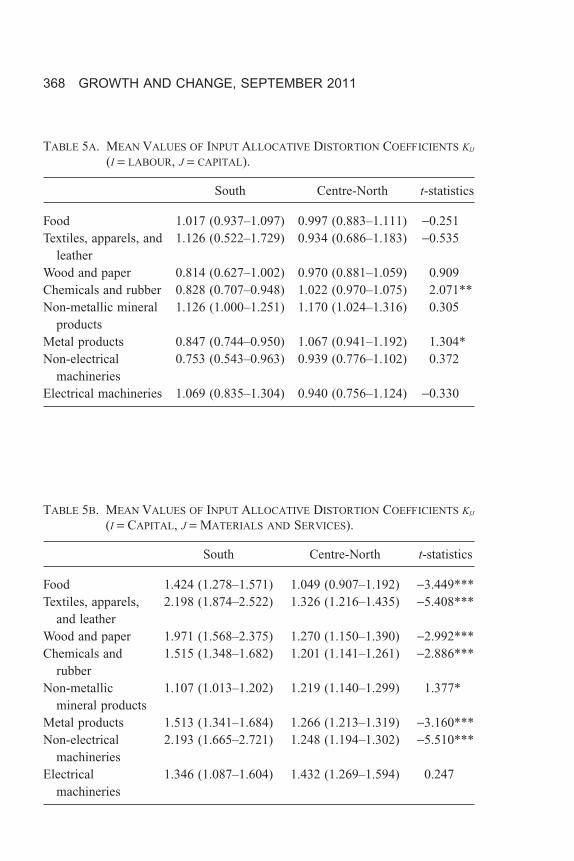
TABLE 5A. MEAN VALUES OF INPUT ALLOCATIVE DISTORTION COEFFICIENTS KIJ

(I = LABOUR, J = CAPITAL).


Food 1.017 (0.937–1.097) 0.997 (0.883–1.111) -0.251Textiles, apparels, and

leather1.126 (0.522–1.729) 0.934 (0.686–1.183) -0.535

Wood and paper 0.814 (0.627–1.002) 0.970 (0.881–1.059) 0.909Chemicals and rubber 0.828 (0.707–0.948) 1.022 (0.970–1.075) 2.071**Non-metallic mineral

products1.126 (1.000–1.251) 1.170 (1.024–1.316) 0.305

Metal products 0.847 (0.744–0.950) 1.067 (0.941–1.192) 1.304*Non-electrical

machineries0.753 (0.543–0.963) 0.939 (0.776–1.102) 0.372

Electrical machineries 1.069 (0.835–1.304) 0.940 (0.756–1.124) -0.330

TABLE 5B. MEAN VALUES OF INPUT ALLOCATIVE DISTORTION COEFFICIENTS KIJ

(I = CAPITAL, J = MATERIALS AND SERVICES).


Food 1.424 (1.278–1.571) 1.049 (0.907–1.192) -3.449***Textiles, apparels,

and leather2.198 (1.874–2.522) 1.326 (1.216–1.435) -5.408***

Wood and paper 1.971 (1.568–2.375) 1.270 (1.150–1.390) -2.992***Chemicals and

rubber1.515 (1.348–1.682) 1.201 (1.141–1.261) -2.886***

Non-metallicmineral products

1.107 (1.013–1.202) 1.219 (1.140–1.299) 1.377*

Metal products 1.513 (1.341–1.684) 1.266 (1.213–1.319) -3.160***Non-electrical

machineries2.193 (1.665–2.721) 1.248 (1.194–1.302) -5.510***

Electricalmachineries

1.346 (1.087–1.604) 1.432 (1.269–1.594) 0.247


and finds significant capital over-utilisation in Southern manufacturing firms in1989–1997. However, because of the different approaches adopted, the differenttime spans and the imposition of alternative assumptions on the technology, theseresults are not directly comparable with the results in this paper.

The kk,cms coefficients appear statistically greater than 1 for both the groups.This result is interesting and suggests that, with a few exceptions, capital issignificantly under-utilised with respect to variable inputs (typically, materials andservices). Considering the regional differences, in almost all industries, Southernfirms appear to be affected by a greater misallocation than their counterparts at the1 percent statistical level. There are two aspects that need to be considered.

First, this finding is consistent with the growing trend toward deverticalisationthat characterised manufacturing in the North of Italy from the 1970s (Traù 1999;Trento 2003) and more recently applied also to the Central and Southern regions(Giunta and Scalera 2006). Deverticalisation and contracting out processes,

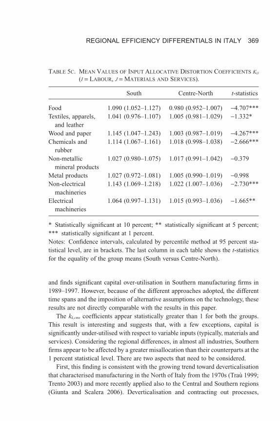
TABLE 5C. MEAN VALUES OF INPUT ALLOCATIVE DISTORTION COEFFICIENTS KIJ

(I = LABOUR, J = MATERIALS AND SERVICES).


Food 1.090 (1.052–1.127) 0.980 (0.952–1.007) -4.707***Textiles, apparels,

and leather1.041 (0.976–1.107) 1.005 (0.981–1.029) -1.332*

Wood and paper 1.145 (1.047–1.243) 1.003 (0.987–1.019) -4.267***Chemicals and

rubber1.114 (1.067–1.161) 1.018 (0.998–1.038) -2.666***

Non-metallicmineral products

1.027 (0.980–1.075) 1.017 (0.991–1.042) -0.379

Metal products 1.027 (0.972–1.081) 1.005 (0.990–1.019) -0.998Non-electrical

machineries1.143 (1.069–1.218) 1.022 (1.007–1.036) -2.730***

Electricalmachineries

1.064 (0.997–1.131) 1.015 (0.993–1.036) -1.665**

* Statistically significant at 10 percent; ** statistically significant at 5 percent;*** statistically significant at 1 percent.Notes: Confidence intervals, calculated by percentile method at 95 percent sta-tistical level, are in brackets. The last column in each table shows the t-statisticsfor the equality of the group means (South versus Centre-North).


fostering the creation of networks of vertical supply relationships, are generallyclaimed to allow Italian firms reduce their asset structures and to make savings onlabour and capital costs. However, few studies have investigated whether thesestrategies actually improve firm performance. Our findings show that deverticali-sation generally leads to excess external purchases, thus violating allocativeefficiency conditions.

Second, the evidence of higher capital under-utilisation for Southern firmsseems consistent with their specialisation in traditional productions based onlow-level technologies. One way to stimulate capital investments (and conse-quently capital cost sharing) might be to address major efforts to improvingcapital quality through multi-level investment programmes, which, in turn, wouldrequire strong commitment on the part of both firms and government. Obviously,this would also require a more efficient credit market and the removal of rigiditiesin the allocation of financial resources.

In relation to kl,cms coefficients, labour appears under-utilised with respect toexternal costs only in the South. The results of the distortion coefficients byindustry reveal a greater, and generally significant, potential for Southern firms toachieve higher cost savings through a reduction in the external supplies cost shareand a simultaneous increase in the labour cost share. In addition, six industriesshow statistically significant differences in group means, which reveal a greaterdistortion in the South. This may in part be attributed to the above-mentionedtendency for under-investment. Also, this finding is in line with the—in somecases dramatically—high unemployment rates experienced in the South and withthe persistent mismatch between the two sides of the local labour market.

Finally, we note that in only a few cases—specifically related to the labour-capital mix—does the allocative distortion assume opposite directions for the twogeographical groups being considered. This indicates a common tendency in therelative over- or under-utilisation indices.

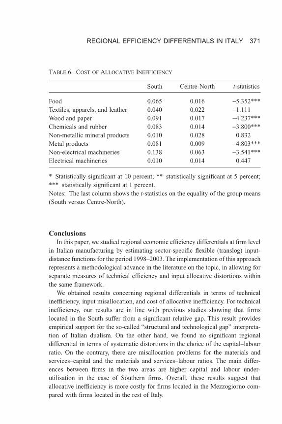
The above results indicate that the input mix is generally inefficient and thatfirms could achieve higher cost performance through a more efficient allocation ofinputs. The next step, therefore, is to determine the cost of allocative efficiency inboth geographical groups. Table 6 presents the estimates of allocative inefficiency.The last column in the table reports the mean comparison t-test between the twogroups. The results generally show that allocative inefficiency increases cost morefor Southern firms. The difference between the two geographic areas is statisti-cally significant at the 1 percent level in five cases, with a gap ranging from1.8 percent to 7.5 percent. This result would suggest that firms located in the Southsuffer from excess costs due to non-optimal input allocation in addition to tech-nical inefficiency.


ConclusionsIn this paper, we studied regional economic efficiency differentials at firm level

in Italian manufacturing by estimating sector-specific flexible (translog) input-distance functions for the period 1998–2003. The implementation of this approachrepresents a methodological advance in the literature on the topic, in allowing forseparate measures of technical efficiency and input allocative distortions withinthe same framework.

We obtained results concerning regional differentials in terms of technicalinefficiency, input misallocation, and cost of allocative inefficiency. For technicalinefficiency, our results are in line with previous studies showing that firmslocated in the South suffer from a significant relative gap. This result providesempirical support for the so-called “structural and technological gap” interpreta-tion of Italian dualism. On the other hand, we found no significant regionaldifferential in terms of systematic distortions in the choice of the capital–labourratio. On the contrary, there are misallocation problems for the materials andservices–capital and the materials and services–labour ratios. The main differ-ences between firms in the two areas are higher capital and labour under-utilisation in the case of Southern firms. Overall, these results suggest thatallocative inefficiency is more costly for firms located in the Mezzogiorno com-pared with firms located in the rest of Italy.

TABLE 6. COST OF ALLOCATIVE INEFFICIENCY


Food 0.065 0.016 -5.352***Textiles, apparels, and leather 0.040 0.022 -1.111Wood and paper 0.091 0.017 -4.237***Chemicals and rubber 0.083 0.014 -3.800***Non-metallic mineral products 0.010 0.028 0.832Metal products 0.081 0.009 -4.803***Non-electrical machineries 0.138 0.063 -3.541***Electrical machineries 0.010 0.014 0.447

* Statistically significant at 10 percent; ** statistically significant at 5 percent;*** statistically significant at 1 percent.Notes: The last column shows the t-statistics on the equality of the group means(South versus Centre-North).


In terms of policy recommendations, business incentives, contrasting declin-ing efficiency due to deverticalisation, would seem to be needed, especiallyaimed at the more depressed Southern regions, although the implementationof business incentives programmes alone will not be sufficient to close theregional gap. Our results highlight that the recently observed tendency to adoptpolicy instruments based mainly on business incentives is likely to be ineffec-tive in the absence of a stronger commitment to narrowing the structuralregional gap.

NOTES1. The Mezzogiorno area includes the Southern Italian regions of Sicilia, Sardegna, Puglia, Cam-

pania, Molise, Calabria, Abruzzo, and Basilicata. With the exception of Molise and Abruzzo, in

the 2000–2006 Community Support Framework, the Mezzogiorno regions belonged to the objec-

tive 1, as all have a per capita income of less than 75 percent of the European level. The objectives

of the programming period 2007–2013 include Calabria, Campania, Puglia, and Sicilia: “conver-

gence objective”; Basilicata: “statistical phasing-out”; Sardegna: “phasing-in”; Molise and

Abruzzo: “competitiveness and employment objective.”

2. For a survey of the different stages of public intervention in the Mezzogiorno, see Del Monte and

Giannola (1997).

3. In a former configuration of the supply-based policy (in roughly 1950–1992), development

strategies typically followed a “top-down” approach that required full centralisation at national

level of any public intervention. The National Agency for Mezzogiorno (Cassa per il Mezzo-

giorno) was responsible for both planning and funding processes until 1992. The main interven-

tion lines within industrialisation policies were 1) public investment in infrastructure, 2) public

investment in state-owned enterprises, and 3) the funding of private investment in the form of both

capital and interest contributions.

4. A great deal of confidence is placed in the so-called “productive” role of public spending, i.e.,

public spending oriented toward the provision of public goods that brings about an externality

effect and enhanced growth by raising private sector productivity. Because the seminal contribu-

tions of Aschauer (1989) and Barro (1990), the contribution of government expenditure in

infrastructures to the productivity of private factors of production and to economic growth has

been heavily investigated. For a comprehensive survey of the empirical evidence, see Romp and

De Haan (2007).

5. Business incentives are regulated by a number of different laws. They differ in terms of the

duration of incentives (from short term to permanent) and targeted variables (employment,

innovation, and investment). For the manufacturing sector, they can be grouped into interest rates

subsidies, and capital grants and tax credits (Destefanis and Storti 2005).

6. The allocative distortion may originate from socio-economic or regulatory constraints placed by

governments on producers as well as—as argued above—from particular environmental features,

or more simply from pure managerial allocative inefficiency.

7. The disaggregation of the sample was carried out bearing in mind the potential trade-off between

the need to have homogeneous groups and the risk associated with small-sample bias. More details

on the composition of the sample are provided in the later section.


8. A single-output technology might be modelled using a production frontier (see the study by Harris

2001 where a stochastic frontier production function is used to derive estimates of technical

efficiency for several UK manufacturing industries). Unfortunately, this approach does not allow

us to make inferences about the allocative distortion in the use of the inputs.

9. The input distance function, ranging from 1 to infinity, is the inverse of the input-oriented Farrell

(1957) technical efficiency measure, which ranges from 0 to 1.

10. For details of the calculation of this overall measure of cost of allocative inefficiency, see

Rodríguez-Álvarez, Fernández-Blanco, and Lovell (2004). Optimisation was performed in

MATLAB using values (1,1,1) as starting points. Inputs were normalised on the operating cost of

materials and services.

11. The translog is a flexible functional form which minimises the a priori restrictions on the

technology.

12. Because of the singularity of the covariance matrix, one of the cost share equations was dropped.

The results are not affected by the choice of which share equation to drop. As one of the aims of

this study is to analyse the coefficients of allocative distortion for each input pair, the model was

run twice, dropping one share equation at a time. This allowed us to obtain estimates of the

parameters of all three share equations and consequently of all the kij allocative inefficiency

indices.

13. We checked curvature conditions on the basis of estimated coefficients, and concavity of the

input distance function in the inputs was satisfied for all the industries at the sample mean

point.

14. See Rodríguez-Álvarez, Fernández-Blanco, and Lovell (2004) for a similar approach. The result-

ing technical efficiency scores may be underestimated because of the fact that all time-invariant

factors (with the exception of those explicitly included in the model) are picked up by the

fixed-effects terms. However, assuming that the persistent effects associated with pure time-

invariant heterogeneity are equally distributed between the two macro-regions, the regional com-

parison would be substantially unaffected.

15. Bottasso and Conti (2010) apply a similar approach to the case of the airport industry in the

UK.

16. We used two different value-added industry deflators for Southern and Centre-Northern areas.

17. Using a fixed-effects specification, we avoid the assumption of individual characteristics (which

capture most of the effects influencing inputs choice) being uncorrelated with the input regressors.

18. Estimates from the 3SLS are not presented here, but they largely confirm the results discussed.

Results are available upon request.

19. Technical change for the South may be calculated simply as the sum of dt and dtSOUTH (the standard

errors may also be recomputed using the delta method). Comparison of technical change in the

two macro-regions is not presented because it is redundant with respect to the estimates presented

in Table 3.

20. Following the approach proposed by Schmidt and Sickles (1984), the technical efficiency scores

were obtained as exp{-(max(hm) - hm)}.

21. According to the arguments in note 16, the magnitude of technical efficiency should be evaluated

with some caution. Bottasso and Sembenelli (2004) obtain higher efficiency scores (ranging

between 0.902 and 0.989) applying a stochastic production frontier approach with year- and

firm-specific inefficiency disturbance component.


REFERENCESAschauer, D.A. 1989. Is public expenditure productive? Journal of Monetary Economics 23(2):

177–200.

Atkinson, S.E., C. Cornwell, and O. Honerkamp. 2003. Measuring and decomposing productivity

change: Stochastic distance function estimation versus data envelopment analysis. Journal of

Business & Economic Statistics 21(2): 284–294.

Barca, F. 2003. Rethinking development policies in Italy. In The Italian economy at the dawn of the

21st century, ed. M. Di Matteo, and P. Piacentini, 129–149. Aldershot: Ashgate.

———. 2006. European Union evaluation between myth and reality: Reflections on the Italian

experience. Regional Studies 40(2): 273–276.

Barro, R.J. 1990. Government spending in a simple model of endogenous growth. Journal of Political

Economy 98(5): S103–S126.

Bottasso, A., and M. Conti. 2010. An assessment on the cost structure of the UK airport industry:

Ownership outcomes and long run cost economies. Department of Economics and Public Finance

“G. Prato” Working Paper Series No. 13. University of Turin.

Bottasso, A., and A. Sembenelli. 2004. Does ownership affect firms’ efficiency? Panel data evidence

on Italy. Empirical Economics 29(4): 769–786.

Capitalia. 2002. Indagine sulle imprese manifatturiere. Ottavo rapporto sull’industria italiana e sulla

politica industriale. Rome.

———. 2005. Indagine sulle imprese manifatturiere. Nono rapporto sull’industria italiana e sulla

politica industriale. Rome.

Cenci, M., and M. Scarlato. 2002. Istituzioni e mercato del lavoro nel Mezzogiorno d’Italia: un’analisi

dinamica. Rivista di Politica Economica 92(5/6): 281–320.

Coelli, T., and S. Perelman. 2000. Technical efficiency of European railways: A distance function

approach. Applied Economics 32(15): 1967–1976.

Costabile, L., ed. 1996. Istituzioni e sviluppo economico del Mezzogiorno. Bologna: il

Mulino.

Del Monte, A., and A. Giannola, eds. 1997. Istituzioni economiche e Mezzogiorno. Roma: Nuova Italia

Scientifica.

Destefanis, S. 2001. Differenziali territoriali di produttività ed efficienza negli anni 90: I livelli e

l’andamento. CELPE Discussion Paper 59, University of Salerno.

Destefanis, S., and G. Storti. 2005. Evaluating business incentives through DEA. An analysis of

Capitalia firm data. DISES Working Paper 3.173, University of Salerno.

Färe, R., and S. Grosskopf. 1990. A distance function approach to price efficiency. Journal of Public

Economics 43(1): 123–126.

Färe, R., and D. Primont. 1995. On inverse homotheticity. Bulletin of Economic Research 47(2):

161–166.

Farrell, M.J. 1957. The measurement of productive efficiency. Journal of the Royal Statistical Society

120(3): 253–290.

Giannola, A. 2002. Il credito difficile. Napoli: L’Ancora del Mediterraneo.

Giannola, A., and C. Petraglia. 2006. Efficienza tecnica e di costo dell’impresa meridionale: frontiere

deterministiche e stocastiche a confronto. In Riforme e mutamento strutturale in Italia, ed. A

Giannola, 133–166. Roma: Carocci editore.


Giunta, A., and D. Scalera. 2006. Le relazioni di subfornitura tra le imprese in Italia. Uno studio

sull’evoluzione degli anni novanta. In Riforme e mutamento strutturale in Italia, ed. A. Giannola,

167–190. Roma: Carocci editore.

Grosskopf, S., K.J. Hayes, L.L. Taylor, and W.L. Weber. 2001. On the determinants of school district

efficiency: Comparison and monitoring. Journal of Urban Economics 49(3): 453–478.

Hadi, A.S. 1994. A modification of a method for the detection of outliers in multivariate samples.

Journal of the Royal Statistical Society Series B 56(2): 393–396.

Harris, R.I.D. 2001. Comparing regional technical efficiency in UK manufacturing plants: The case of

Northern Ireland 1974–1995. Regional Studies 35(6): 519–534.

ISAE. 2003. I rapporti banca-impresa e I vincoli finanziari alla crescita delle piccolo e medie imprese.

Rapporto, and A 2003. Priorità nazionali: dimensioni aziendali, competitività, regolamentazione.

Rome.

Ministero dello Sviluppo Economico. 2006. Relazione sugli interventi di sostegno alle attività eco-

nomiche e produttive. Rome.

Morone, P., C. Petraglia, and G. Testa. 2007. Research, knowledge spillovers and innovation: Evidence

for the Italian manufacturing sector. Birkbeck Working Papers in Economics and Finance 0703,

Birkbeck, University of London.

Nickell, S., and D. Nicolitsas. 1999. How does financial pressure affect firms? European Economic

Review 43(8): 1435–1456.

Rodríguez-Álvarez, A., and C.A.K. Lovell. 2004. Excess capacity and expense preference behaviour

in national health systems: An application to the Spanish public hospitals. Health Economics

13(2): 157–169.

Rodríguez-Álvarez, A., V. Fernández-Blanco, and A.K. Lovell. 2004. Allocative inefficiency and its

cost: The case of Spanish public hospitals. International Journal of Production Economics 92(2):

99–111.

Romp, W., and J. De Haan. 2007. Public capital and economic growth: A critical survey. Perspektiven

der Wirtschaftspolitik 8(S1): 6–52.

Sarno, D. 2003. Un modello di razionamento del credito operativo alle imprese: Il caso delle piccole

e medie imprese del Mezzogiorno. Economia Politica 20(3): 371–390.

Schmidt, P., and C.A.K. Lovell. 1979. Estimating technical and allocative inefficiency relative to

stochastic production and cost frontiers. Journal of Econometrics 9(3): 343–366.

Schmidt, P., and R.C. Sickles. 1984. Production frontiers and panel data. Journal of Business and

Economic Statistics 2(4): 367–374.

Shephard, R.W. 1953. Cost and production functions. Princeton: Princeton University Press.

Traù, F. 1999. La discontinuità dei pattern di sviluppo dimensionale delle imprese nei paesi indistriali:

fattori endogeni ed esogeni di mutamento dell’ambiente competitivo. Working Paper Centro Studi

Confindustria 19. Roma: Confindustria.

Trento, S. 2003. Stagnazione e frammentazione produttiva. Il Mulino 6: 1093–1102.


Documents

Drivers of Regional Efficiency Differentials in Italy: Technical Inefficiency or Allocative Distortions?