Embed Size (px)
Citation preview

DEPARTMENT OF MECHANICS AND MARITIME SCIENCE
CHALMERS UNIVERSITY OF TECHNOLOGY
Gothenburg, Sweden 2021
www.chalmers.se
Driver Modelling for Virtual Safety Assessment of Automated Vehicle Functionality in Cut-in Scenarios Accumulation Model Development Using SHRP2 Data
Master’s thesis in Automotive Engineering
CHRISTOFFER CHAU QIANYU LIU


MASTER’S THESIS IN PROGRAMME NAME
Driver modelling for safety assessment of automated
vehicle functionality in cut-in scenarios
Christoffer Chau
Qianyu Liu
Department of Mechanics and Maritime Sciences
Division of vehicle safety
CHALMERS UNIVERSITY OF TECHNOLOGY
Göteborg, Sweden 2021

Driver modelling for virtual safety assessment of
automated vehicle functionality in cut-in scenarios
Christoffer Chau
Qianyu Liu
© Christoffer Chau & Qianyu Liu, 2021-07-08
Supervisor: Jonas Bärgman, Mechanics and Maritime Sciences
Examiner: Jonas Bärgman, Mechanics and Maritime Sciences
Master’s Thesis 2021:55
Department of Mechanics and Maritime Sciences
Division of vehicle safety
Chalmers University of Technology
SE-412 96 Göteborg
Sweden
Telephone: + 46 (0)31-772 1000
Cover:
Graphical representation of cut-in scenario: a vehicle (blue) from adjacent lane is
cutting in the front of the orange vehicle. The driver model developed in this thesis aims
to predict the braking response of the vehicle (orange) being cut-in. Detailed
descriptions of the cut-in scenario can be found in Section 1.2 and 2.1.
Department of Mechanics and Maritime Sciences
Göteborg, Sweden 2021-07-08

Driver modelling for virtual safety assessment of
automated vehicle functionality in cut-in scenarios
Christoffer Chau
Qianyu Liu
Department of Mechanics and Maritime Sciences
Division of Vehicle Safety
Unit of Crash Analysis and Prevention
Chalmers University of Technology
Abstract
The development of active safety systems and automated vehicles has increased
exponentially in recent years and can influence traffic safety in various ways.
Prospective assessments of their safety impacts are required during the development of
active safety systems and automated vehicle functionality. Virtual simulation is one of
the most common approaches of safety prospective assessments; a method that uses
models to represent drivers, vehicles and road environments, etc., and run simulations
in computers to estimate the risk and benefit of safety systems. This thesis aims to
extend and implement an existing rear-end accumulation driver model into a cut-in
driver model in the virtual simulation tool Esmini. The model is for predicting the
braking behaviour of the driver of a vehicle (going straight, denoted EGO vehicle) when
another vehicle (denoted Principle Other Vehicle; POV) from an adjacent lane is cutting
in in the front of the EGO vehicle. The model parameters were optimized to cut-in near-
crashes from a set of Naturalistic Driving Data from The Second Strategic Highway
Research Program (SHRP2) in the US. The stochastic machine learning method Particle
Swarm Optimization was used to fit the braking onset timing and jerk, which represent
the time when a driver starts to decelerate harshly and the ramp-up of the deceleration,
respectively, as defined by a piecewise linear model of the behaviour observed in the
SHRP2 data. Three different models were introduced and implemented in the virtual
simulation framework. The performance of the models were good for some events, but
could not capture the variability across all events sufficiently for direct use in safety
assessment. Future work could include fitting the model to more data, as well as fixing
some parameters to reduce the complexity of the current model and capturing more
information, which could affect the driver response in a cut-in scenario. With further
developments of the models, it may be used for safety assessment of active safety or
other vehicle automation functions.
Key words: Driver model, Cut-in scenario, SHRP2, Naturalistic Driving Data,
Automated vehicle, Particle swarm optimization, Virtual simulation, Active safety


Contents
Abstract ............................................................................................................................................ I
Contents ........................................................................................................................................ III
Preface ............................................................................................................................................. V
Acknowledgements .................................................................................................................... V
Notations ...................................................................................................................................... VI
1 Introduction.............................................................................................................................. 1
1.1 Accumulation driver model ........................................................................................ 4
1.2 Aim and objectives ......................................................................................................... 6
2 Methodology ............................................................................................................................. 8
2.1 Events selection and annotation .............................................................................. 8
2.2 Data processing .............................................................................................................12
2.3 Cut-in driver model .....................................................................................................16
2.3.1 Model 1 ....................................................................................................................17
2.3.2 Model 2 ....................................................................................................................17
2.3.3 Model 3: ...................................................................................................................19
2.3.4 Kalman Filter for predicting derivatives ....................................................20
2.4 Parameters Optimization ..........................................................................................21
2.4.1 Cost function ..........................................................................................................22
3 Result ........................................................................................................................................26
3.1 Training without noise ...............................................................................................26
3.1.1 Model 1 - without noise .....................................................................................26
3.1.2 Model 2 - without noise .....................................................................................27
3.1.3 Model 3 - without noise .....................................................................................28
3.1.4 Model comparison ...............................................................................................29
3.1.5 Results from the best model – Model 3 .......................................................31
3.2 Training with noise – Model 3 .................................................................................33
4 Discussions .............................................................................................................................35
4.1 Interpretation of results ............................................................................................35
4.1.1 Compare the models ...........................................................................................35
4.1.2 Likely reasons to why the driver model does not fully capture the driver's behaviour ................................................................................................................37
4.2 Methodological choices ..............................................................................................38
4.3 Limitations and Future work ...................................................................................39
5 Conclusion ...............................................................................................................................41

6 References ...............................................................................................................................42
Appendix ...........................................................................................................................................44

Preface
This research is a master thesis work carried out at the Department of Mechanics and
Maritime Sciences, Division of Vehicle Safety, Chalmers University of Technology,
Sweden. The work was developed from January to August 2021, and part of the work
was performed at the offices of the Vehicle and Traffic Safety Centre at Chalmers –
SAFER, Gothenburg.
Acknowledgements
First, we would like to thank our examiner and supervisor Jonas Bärgman for his
tremendous support throughout the thesis. Without your support, we don’t think we
would have made it this far. Not only did you support us with the research but also
giving us advice for the future and we are extremely grateful for that. A special thanks
to Giulio Bianchi Piccinini and Marco Dozza for your feedback during mid-
presentation. In addition, we would like thank Xiaomi and Pierluigi for your advices
and support on our research work. We would also like to thank SAFER for offering us
a nice work environment.
We want to thank VTTI for sharing SHRP2 data with us in this research and permission
for showing pictures in the report and presentation. We also want to thank esmini team
for providing a free and open source simulation tool. A special thanks to Emil Knabe
of his assistance in resolving Esmini-related issues. We would like to thank Riyam
Tayeh, Ahmed Shams El Din, and Vignesh Krishnan from Volvo Cars for providing us
the code to run Esmini.
We wish to thank all our friends, the ones we met in Sweden from all over the world
and also our old friends, who are always be supportive during hard times. A special
thanks to Kishore for all the discussions about related topics during coffee breaks. Last
but not least, we would like to thank all our families who have supported us throughout
our studies and been believing in us all the time.
This work has been performed under the VTTI SHRP2 Data License Agreement. The
findings and conclusions of this report are those of the author(s) and do not necessarily
represent the views of VTTI, the Transportation Research Board, or the National
Academies. The data used falls within the licence agreement SHRP2-DUL-A-16-204
and the data has the DOI:10.15787/VTT1K013.
Göteborg March 2021-07-08
Christoffer Chau & Qianyu Liu
Notations
AS Activity Safety
GUI Graphical User Interface
POV Principle Other Vehicle – the vehicle which the EGO vehicle
is in conflict
EGO The vehicle with the driver model, also known as the subject
vehicle
SHRP2 Second Strategic Highway Research Program
NDD Naturalistic Driving Data
VAT Video Annotation Tool
PSO Particle Swarm Optimization
GA Genetic Algorithm
ADAS Advance Driving Assistance System
AD Automated Driving
VTTI Virginia Tech Transportation Institute
FOT Field Operational Test
DAS Data Acquisition System
Euro NCAP European New Car Assessment Programme
TTC Time To Collision
Before POV-in-lane The condition that the POV is completely outside the EGO
vehicle’s lane (has not crossed the lane marking)
After POV-in-lane The condition that the POV is overlapping with the EGO
vehicle’s lane lane-marking, or the POV being inside the same
lane as EGO vehicle
AIC Akaike Information Criterion
𝑡𝐵 Break onset timing - time when the driver started to break
harshly
𝑗𝐵 Jerk - ramp up of the acceleration

CHALMERS, Mechanics and Maritime Sciences, Master’s Thesis 2021:55 1
1 Introduction
In 2019 there were approximately 1.35 million fatalities and between 20 and 50 million
people suffered non-fatal injuries (WHO 2020). As a result, road traffic accidents put a
huge strain on all nations, both from an economic and social perspective (Markkula,
2014). Humans are the main reason why accident occur in the first place, and much
research has been conducted to understand human behaviour in traffic and how to
improve safety or avoid accident (Markkula et al., 2012). New active safety systems,
advanced driving assistance systems (ADAS) and automated driving (AD)
functionality have been developed to reduce the number and severity of accidents, and
to help human drivers avoiding dangerous situation. These ADASs and ADs will help
drivers to avoid or mitigate crashes by partially taking over the vehicle when the driver
loses control, or they may send warning signals to alert the driver of imminent threats.
The development of safety-relevant functions necessitates a quantitative assessment of
their impact on traffic safety, taking into account both positive and negative aspects
(Helmer et al., 2015). There are two types of assessment approaches: prospective
assessment and retrospective assessment. The goal of retrospective assessment is to
quantify the benefits or risks introduced by an ADAS or AD function after it has been
in use in market for a period. Prospective assessment, on the other hand, is aimed to
predict the effectiveness and expected safety benefits of a new functions.
Field Operational Tests (FOT), test tracks, driving simulators, accident analysis, and
virtual simulations are the most commonly used prospective safety assessment
approaches (Page et al., 2015). In FOT, the ADAS or AD functions are installed on
vehicles and tested in real-world traffic. Because it involves normal drivers and real-
world traffic situations, the FOT approach can produce robust and comprehensive
results. However, it necessitates a significant amount of resources and comes at a high
cost. In the test track approach, the functions are installed in a vehicle and tested in a
test track with professional drivers under known conditions. In comparison to FOT, test
track can test the functions under critical but controlled situation, avoiding putting
drivers in danger. Because not all conditions can be tested on a test track and the drivers
are professionals, the evaluation results are less reliable than FOT. It is very difficult,
or, often, impossible, to extrapolate test track testing to actual safety benefits. Driving
simulators can capture real driver’s reactions in virtual simulations and enable repeated
testing of new functions. But the fidelity is even lower than test track tests because
drivers may react differently in virtual simulation and in real world. Virtual simulations,
on the other hand, use computers to mimic (simulate) driving, which enable safety
assessments in different scenarios at a reasonable cost, and depending on the data used
as a basis, allows for actual estimates of absolute benefits of the safety system under
assessment. However, using virtual simulation puts high requirements on driver models
to guarantee accuracy and precision in the simulation results (Page et al., 2015).

CHALMERS, Mechanics and Maritime Sciences, Master’s Thesis 2021:55 2
Figure 1 Virtual simulation
Scenario-based virtual assessment is one specific form of virtual simulations, used to
quantify the effectiveness of a function in a specific scenario using simulations. The
overall safety effectiveness is then calculated as the sum of effectiveness of all scenarios
weighted by the frequency of each scenario (Helmer et al., 2015). A simple framework
of virtual simulations is shown in Figure 1. Once the scenario is determined, the input
dataset, which includes a collection of events from critical situations within the context
of the specific scenario, is prepared for virtual simulations. The input dataset can either
be synthetic data generated from the distribution of pre-crash conditions, or
reconstructed from real-world driving data, such as Naturalistic driving data (NDD).
The second Strategic Highway Research (SHRP2) naturalistic driving study is the
largest naturalistic driving study program to date, having captured data about 3,400+
drivers and vehicles during their daily driving, including 36,000 crash and near-crash
events. The Virginia Tech Transportation Institute (VTTI) was the technical
coordination and study design contractor for the SHRP2 naturalistic driving study. The
SHRP2 NDD provides detailed pre-crash, driver behaviours and exposure information,
which can be used for research and develop different safety systems (Gordon &
Srinivasan, 2014). The Data Acquisition System (DAS) used to collect the SHRP2 data
contained a forward radar, four video cameras (including forward view, rear and right
view, driver and left side view and passenger snapshot view), accelerometers
(measuring the acceleration in the longitudinal, lateral and vertical direction),
Geographic Positioning System (GPS), as well as gyroscopes measures (yaw rate, roll
rate and pitch rate) (Virginia Tech Transportation Institute, 2020). To date there are
more than 300 publications that utilize SHRP2 data in one way or another.
The input data generation for use of, for example, SHRP2 data, requires processing of
raw NDD data. The Data Reduction Group from VTTI reduce the raw data into a format
that allows specific research and have developed software tools to analyse eyeglance
and other video-based data (Virginia Tech Transportation Institute, 2021). Further, an
annotation tool was developed in previous work at Chalmers (Din et al., 2020) – a tool
that can extract the distance to lane markings and other vehicles, by manually (semi-
automatically) annotating the forward view video from SHRP2 events. The goal of
developing the tool was to support manual annotation of NDD to extract the necessary
data, such as lane markings, position and movement of the Principe Other Vehicle
(POV; the vehicle with which the instrumented vehicle, called EGO vehicle, is
primarily in conflict), for research.

CHALMERS, Mechanics and Maritime Sciences, Master’s Thesis 2021:55 3
As mentioned earlier, FOTs can be expensive when testing safety systems. Virtual
simulation is a much more cost efficient and safe way of testing safety systems
(Benderius, 2012). However, in virtual simulation, models are needed to represent
drivers, vehicles, etc. Such models can be classified into two types: deterministic and
stochastic. The output of deterministic models is fixed given a specific input and
parameter set, whereas stochastic models produce randomness. There are many
uncertainties in real world, for example different drivers may react differently in a
critical situation and even the same driver may behave differently when exposed to the
same critical situation. Hence, stochastic simulation should preferably be performed on
large representative samples of virtual representations of crashes during the
development and assessment of AS or ADAS functions. Further, computational models
of drivers, vehicles, traffic flow, road environment and their interactions are required
in virtual simulations as the representations of real traffic situations.
There are different driver models, such as driver control behaviour models in near-crash
rear-end scenarios (Markkula, 2014) and models that keep a vehicle in the lane (Gordon
& Srinivasan, 2014). Lee’s (2012) research show how a driver might visually control
his/her braking and how driver may control his/her braking and vehicle-following
behaviour by monitoring the forward scene with the eyes (visually). Therefore,
understanding how drivers visually gather information is important for improvement
on road safety, as it is needed to develop accurate and realistic models of driver
behaviour. Based on theory about visual cues an evidence-accumulation based driver
model for car-to-car rear-end conflict was proposed by Svärd et al. (2017). The Svärd
et al. model used perceptual visual looming to determine how “hard” the driver should
brake to avoid collision. The model was further developed in Svärd et al. (2020). When
developing models and fitting their parameters there is typically a need to have a
framework to perform virtual simulations, so that some set of performance indicators
can be compared between the model and the data it should be fitted to. Examples of
such frameworks are Virtual Test Drive (Hexagon AB, 2021) and OpenPass
(Invisiblefarm s.r.l., 2014). But also the open source simulation software Esmini (Emil
Knabe, 2021) can be used as a basis for such a framework.
In this thesis, a driver model was developed for cut-in scenarios on highways, using
data from the SHRP2 NDD as a basis. According to the European New Car Assessment
Programme (Euro NCAP), a cut-in scenario is when a car from the adjacent lane merges
into the lane in front of another vehicle (e.g., the vehicle which system is being
assessed). Cut-ins happens in everyday driving, and a driver will usually anticipate the
manoeuvre ahead of time and reduce speed accordingly. Chovan et al. (1994) report
that there were approximately 244,000 lane change/merge crashes, that represented 4%
of all crashes in the US, in 1991. In addition, Chovan et al. estimate that 386,000 non-
police reported lane change/merge crashes happened in the US in the same year. As
ADAS and AD functions are developed to handle cut-in events, it is increasingly urgent
to develop models of driver behaviours in cut-in scenarios, for use in prospective virtual
simulations to assess the systems impact on safety. (Shams El Din, 2020a). We have
not found any scientific paper on driver modelling for cut-in scenario, however the rear-
end accumulation driver model introduced in (Svärd et al., 2017) is related and could
be used as the basis of developing driver model for cut-in scenario. The virtual
simulation components required for driver model development are similar to those for
safety assessment (as shown in Figure 1) but the AS and ADAS functions should be
deactivated to ensure that the simulation outputs are independent of AS and ADAS
functions interventions.

CHALMERS, Mechanics and Maritime Sciences, Master’s Thesis 2021:55 4
1.1 Accumulation driver model
An accumulation model of driver responses to critical situations in rear-end scenario
was introduced in Svärd et al. (2017, 2020). The following is a brief overview of the
Svärd et al. (2017) model (illustrated in Figure 2).
Figure 2 Accumulation driver model
In each timestep, the model collects perceptual evidence by noisy accumulation (as
Equation (1) of the discrepancy between actual perceptual input 𝑃(𝑡) and prediction of
it, denoted as 𝑃𝑝(𝑡).
𝑑𝐴(𝑡)
𝑑𝑡= 𝐾 ∗ ℇ(𝑡) − 𝑀 − 𝐶 ∙ 𝐴 + 𝑣(𝑡) (1)
Where ℇ(𝑡) is the total perceptual error, and it can be calculated as:
ℇ(𝑡) = 𝑃(𝑡) − 𝑃𝑝(𝑡) (2)
where 𝐴(𝑡) is the accumulated evidence, called the activity, 𝐾, 𝑀 and 𝐶 are free model
parameters (to be fitted to data). The details of each parameter can be found in (Svärd
et al., 2020). 𝑣(𝑡) is the zero-mean Gaussian white noise with a standard deviation
𝜎√Δ𝑡. Looming 𝜏−1 (as Equation (3)) is inverse of time to collision (TTC) as described
by variables that the human can perceive:
𝜏−1 =��
𝜃 (3)
where 𝜃 is the optical size (horizontal angle) of the POV. The 𝜃 calculation for rear-
end scenario can be seen Figure 3 and in Equation (4):
𝜃 = 2 ∙ tan−1𝑊𝑝𝑜𝑣 2⁄
𝑑𝑥 (4)

CHALMERS, Mechanics and Maritime Sciences, Master’s Thesis 2021:55 5
where 𝑊𝑝𝑜𝑣 is the width of the LV, dx is the longitudinal distance between the POV’s
rear bumper and EGO vehicle’s front bumper.𝜏−1 was used as the models perceptual
input in (Svärd et al., 2017).
Figure 3 Optical size of POV in read-end scenario
Once the activity, 𝐴, exceed a pre-defined threshold, the driver model will issue a brake
signal to the vehicle models brake actuation. The amplitude of the brake adjustment is
determined by a linear function 𝐺(𝑡), as shown in Figure 4, scaled by the brake gain
parameter 𝑘 and prediction error 𝜀(𝑡), which represents the braking increasing linearly
to the target level within the adjustment duration △ 𝑇. After each brake adjustment, the
activity 𝐴 will be reset to a lower value 𝐴𝑟 and prediction 𝑃𝑝(𝑡) will be updated to a
scaled of prediction error with time-varying scaling factor 𝐻(𝑡), as shown in Figure 5.
This is done for every timestep in the simulation.
Figure 4 Plot of G(t)
Figure 5 Plot of H(t)
There are eight free model parameters (𝐾, 𝑀, 𝐶, 𝜎, 𝐴𝑟, 𝑘, Δ𝑇𝑝0, Δ𝑇𝑝1 ) in total in the
Svärd et al. (2017) model. After the 2017 publication, Svärd further developed the
model. In (Svärd et al., 2020) some additional parameters were added (to also account
for glances off road), and the model parameters were fitted to the SHRP2 data using
Particle Swarm Optimization (PSO) – the break onset timing 𝑡𝐵 and jerk 𝑗𝐵 was the
variables which were predicted (which the model should predict). The value of noise
item (𝑣(𝑡) in Equation 1) changed over time, resulting in non-deterministic responses
from driver model. The simulation of each event in each PSO iteration was repeated
1000 times, and different acceleration output was obtained for each iteration. The driver
model acceleration output from each simulation was fitted to a piecewise linear function
to get the break onset timing 𝑡𝐵 and jerk 𝑗𝐵 . The 𝑡𝐵 and 𝑗𝐵 values obtained from
repeating simulations were used to generate a 2D probability distribution. The SHRP2
acceleration values of event 𝑖 were also fitted into the piecewise linear function to
obtain the reference value ( 𝑡𝐵,𝑖,𝑟𝑒𝑓 , 𝑗𝐵,𝑖,𝑟𝑒𝑓 ). The ℓ(𝑡𝐵,𝑖,𝑟𝑒𝑓 , 𝑗𝐵,𝑖,𝑟𝑒𝑓|ℙ𝑗,𝑘) , denotes
likelihood of the reference value with given parameter set ℙ𝑗,𝑘(parameter set of the 𝑗 th
0 T
1
0 Tp0
Tp
1

CHALMERS, Mechanics and Maritime Sciences, Master’s Thesis 2021:55 6
particle in the 𝑘 th iteration), was estimated to calculate the fitness of the model. The
cost function provided in Svärd et al., (2020) was then the total log likelihood of all
events in training set using parameter set ℙ𝑗.𝑘, with compensation of potential outlier
as:
log ℒ (ℙ𝑗.𝑘) =∑ log(𝜌 ∙ ℓ(𝑡𝐵,𝑖,𝑟𝑒𝑓 , 𝑗𝐵,𝑖,𝑟𝑒𝑓|ℙ𝑗.𝑘) + (1 − 𝜌) ∙ 𝑝𝑣)𝑁
𝑖=1 (5)
Where 𝑝𝑣 is the outlier compensation term, that was calculated as:
𝑝𝑣 =1
𝑡𝐵,𝑚𝑎𝑥 ∙ 𝑗𝐵,𝑚𝑎𝑥 (6)
With this method, the parameter set with the highest total log likelihood provides the
best fit of SHRP2 training events.
1.2 Aim and objectives
The aim of this thesis was to develop a computational driver model of driver brake
responses in critical situations where a vehicle (POV) in an adjacent lane cuts-in in
front of the vehicle (EGO) going straight (with the driver model). To make this possible,
understanding driver behaviour in traffic is necessary. To achieve that, a developed
annotation tool from Din et al., (2020) was utilized to extract the vehicle kinematics
from near-crashes from the SHRP2 NDD dataset. The extracted kinematics was used
to reconstruct a set of cut-in events, so that they could be simulated in a simulation
environment (Esmini). The driver braking model was applied to each reconstructed
event, but with the brake response in the original event removed. Results of the model
and the original events were then compared, and the parameters optimized to provide
best overall model fit to the data across all events. The driver model development was
based on previous work on accumulators as part of modelling human behaviour for
rear-end conflicts (Svärd et al., (2017). The parameter fitting/training and simulation
run was done in Python, with Esmini as simulation engine. The parameter optimization
for the driver model was similar to that of the research by Svärd et al. (2020), where
PSO was used. Specifically, the driver model developed in this thesis aims to predict
the braking response of the vehicle being cut-in (i.e., the vehicle going straight),
hereafter known as the EGO vehicle. Note that steering of the EGO vehicle was not
covered in this thesis and only passenger car drivers’ responses to cut-ins were included
in this research. Figure 6 visualizes the cut-in scenario, in which the lead vehicle,
referred to as POV, changes lanes and cuts in front of the following vehicle, referred to
as the EGO vehicle. Based on the original rear-end accumulation model new strategies
to calculate looming, additional functions to trigger/accumulate perceptual input related
to distances or angles, were developed in this thesis, for the model to handle cut-ins
(rather than only rear-ends).

CHALMERS, Mechanics and Maritime Sciences, Master’s Thesis 2021:55 7
Figure 6 Event start and end in a cut-in scenario
To achieve the aim, several objectives needed to be fulfilled along the way. The detailed
objectives were as follows:
• Extract and process the trajectory coordinate from SHRP2 data.
• Develop a cut-in driver model to predict the braking of EGO vehicle for the
scenarios where the POV is entering the EGO vehicle lane from an adjacent
lane, in front of EGO vehicle.
• Implement and further develop on current accumulation model for the cut-in
driver model in Esmini.
• Train the cut-in driver model using the machine learning method particle swarm
optimization (PSO) to fit the SHRP2 driver behaviour to the simulation output
in terms of brake onset timing and jerk.
• Evaluate the cut-in driver model with respect to goodness of fit.
• Compare model approaches/parameterizations.

CHALMERS, Mechanics and Maritime Sciences, Master’s Thesis 2021:55 8
2 Methodology
The method used in this thesis will be explained in detail in this chapter. Figure 7 shows
the work process of the implementation, parameterization, and parameter fitting of the
driver model through virtual simulations, using data from the SHRP2 Naturalistic
Driving Data (NDD) set. The evasive driver’s behaviours were removed from SHRP2
data before fed into simulations. The vehicle and driver models were embedded in the
virtual simulation tool Esmini (Emil Knabe, 2021). Volvo Cars provided a script in
Python code to run Esmini for this research, therefore Esmini was chosen for this thesis.
The accelerations from the driver model outputs were compared to the original SHRP2
acceleration in terms of break onset timing and jerk (a piecewise linear fit was done for
both the model output and the original data). Section 2.1 and 2.2 describe how the
trajectories of vehicles and coordinates of lane markings were extracted from the
SHRP2 NDD. Section 2.3 explains how the rear-end accumulation driver model was
modified to models for cut-in scenario in different ways. Section 2.4 shows the model
parameter optimisation process.
Figure 7 Driver model development
2.1 Events selection and annotation
To ensure that the driver model can represent real-world driver behaviour, it was tested
and optimized using SHRP2 NDD. The forward facing video recordings from SHRP2
were manually annotated with an annotation tool developed during previous student
work ( Shams El Din, 2020b, Shams El Din, 2020b). Figure 8 shows the Graphical User
Interface (GUI) of the annotation tool. The forward-facing video of the selected event
can be played, with the annotator having the option of playing it at normal speed, fast
speed, or frame by frame. By clicking points on a lane mark, the annotation tool can
calculate the relative lateral distance between the lane mark and the EGO vehicle. The
relative distances between POV and EGO vehicle in both longitudinal and lateral
directions can be obtained by drawing a box on POV that covers the POV's rear lamps.
SHRP2NDD
Break onset timing & jerk
from driver model output acceleration
Input Data
States of all traffic participants
Environment
Driver Model
Vehicle Model
Perception
Decision making
Remove evasive driver’s behaviour
Virtual Simulation
Parameterization and parameter fitting of
driver model
Break onset timing & jerk
from SHRP2 acceleration

CHALMERS, Mechanics and Maritime Sciences, Master’s Thesis 2021:55 9
Figure 8 Annotation Tool GUI
Not all the events are suitable for annotation. The lane markings should be clear and
the rear lamps of POV should be visible throughout the cutting-in process. Before
annotation, the forward-facing videos of 209 cut-in events from SHRP2 were manually
viewed to remove the events that were not suitable for annotation. Inclusion and
exclusion criteria for annotation of events can be found in Table 1. Inclusion criteria
represent all the necessary criteria that needed to be fulfilled (included in the event),
while exclusion criteria represent possible factors or characteristics of an event that
were excluded as they either were not needed in the modelling or made it difficult to
make the events consistent. That is, events that did not fit the scenario which the model
is sought to represent.
Table 1 Criteria for events selection
Inclusion criteria
• Fully visible rear-lamp of POV
before start of the event
• Clear lane markings throughout
the event
• POV clearly visible throughout
the event
Exclusion criteria
• Non cut-in events
• EGO steering
• EGO changing lane
• Lane merging or splitting
A visualization from a bird view perspective of non-cut-in events, EGO steering to
avoid collision and EGO changing lane, can be seen in Figure 9.

CHALMERS, Mechanics and Maritime Sciences, Master’s Thesis 2021:55 10
Figure 9 Demonstration of exclusion criteria
Lane marks have a very important role in the driver model in cut-in scenarios. The
driver will respond differently depending on the position of the POV. The timing of
when the POV is entering the EGO lane or touching the lane marking will impact the
way the driver responds. A more detailed explanation of POV-in-lane is presented in
the data-processing section. Since the lane marks have an important role, this can
generate some potential problems when the lane marks are missing or not the same as
real-world traffic (e.g., through issues in the annotation process) when generated in
simulation. There were a couple of occasions where lane merging or lane splitting
meant there were no lane marks, see Figure 10. In this event, the EGO lane is splitting
into two different and the POV is cutting in from the right. The user (annotator) has to
“assume” where the lane marks might be located and try to fill the missing gap and
could potentially cause some mismatch between front view video and annotation
output. Consequently, such events were removed.
Figure 10 Lane splitting

CHALMERS, Mechanics and Maritime Sciences, Master’s Thesis 2021:55 11
Missing data is inevitable and was bound to happened. There are events with no
RADAR data and events with RADAR data, see Figure 11 (left upper and lower) for
events with no RADAR data and Figure 11 (right upper and lower) events with RADAR
data. Annotated data is marked with red dotted line (Figure 11 left upper and lower),
while raw data (data from RADAR) is marked with normal lines with different colours
(Figure 11 right upper and lower). Each colour describes the radar range from the ego
vehicle to one (other) individual vehicle. Multiple colours indicate there are multiple
vehicles in front of the EGO vehicle (can be in the ego vehicles lane, or in the adjacent
lanes). This could be problematic if there are many vehicles in front and finding the
correct vehicle will be hard. Luckily, this can be solved by finding which line is closest
to the dotted line (annotated data) and then the user will know which is the correct
vehicle. Another potential problem is the differences in longitudinal distance
(longitudinal offset) between annotated data and RADAR data. This can cause a
mismatch between simulation and the real event from SHRP2.
To find the longitudinal offset, only the top left and the top right figure (Range on the
y axes) in Figure 11 are interesting. By not having any raw data, the annotators will
have a hard time to compare if the annotation (box of the vehicle) is correct or not, with
respect to the estimate of longitudinal distance to the POV. With RADAR data,
annotators can compare the RADAR range and the range estimated from the annotation,
and check if the result looks reasonable or not (see Figure 11, right picture). This
information can later be used to eliminate any large offset from the real data in data
processing (note that the RADAR typically only captured the vehicle late in the cut-in
process, and not actually the lateral motion towards the lane).
Figure 11 RADAR data example. The dashed line is the annotated data. Left X, right Y
Acceleration is another important piece needed for development of driver model. The
data is crucial for acceleration fitting to find the reference value 𝑡𝐵,𝑖,𝑟𝑒𝑓 and 𝑗𝐵,𝑖,𝑟𝑒𝑓 from
the model. A more detailed explanation can be found in section acceleration fitting
(Section 2.1.1.1). By following the criteria presented in Table 1, remaining events were
down to 51 and following the criteria presented in Table 1, only 18 events was selected
out of 51.

CHALMERS, Mechanics and Maritime Sciences, Master’s Thesis 2021:55 12
2.2 Data processing
After selection of the events from SHRP2, the output from the annotation tool needed
to be converted into another data format to be able to run the Esmini simulation. All
coordinates, extracted from the annotation tool, were after annotation in the EGO
vehicle coordinate system, denoted with superscript 𝑣. To enable usage of the data in
Esmini simulations, the coordinates needed to be converted from the local (EGO
vehicle) coordinate system into global coordinates, denoted with superscript 𝑔 , as
shown in Figure 12.
Figure 12 Coordinate conversion
In the longitudinal direction, the positions of the EGO vehicle were calculated by
integrating the CAN speed from SHRP2 data as:
𝑋𝐸𝐺𝑂𝑔
= ∫𝑣𝑥,𝐸𝐺𝑂 𝑑𝑡 (7)
The x coordinates of POV and lane markings were then calculated as:
𝑋𝑃𝑂𝑉𝑔
= 𝑋𝐸𝐺𝑂𝑔
+ 𝑋𝑃𝑂𝑉𝑣 + 𝑙𝑓,𝐸𝐺𝑂 + 𝑙𝑟,𝑃𝑂𝑉 (8)
𝑋𝑙𝑒𝑓𝑡 𝑙𝑎𝑛𝑒𝑔
= 𝑋𝑃𝑂𝑉𝑔
(9)
𝑋𝑟𝑖𝑔ℎ𝑡 𝑙𝑎𝑛𝑒𝑔
= 𝑋𝑃𝑂𝑉𝑔
(10)

CHALMERS, Mechanics and Maritime Sciences, Master’s Thesis 2021:55 13
In the lateral direction, the global coordinates can be obtained by assuming that the
centre of the lane is straight:
𝑌𝑙𝑎𝑛𝑒 𝑐𝑒𝑛𝑡𝑒𝑟𝑔
= 0 (11)
Hence, the y-coordinates of the left lane, right lane, EGO and POV, in global
coordinate system, can be calculated as:
𝑌𝑙𝑒𝑓𝑡 𝑙𝑎𝑛𝑒𝑔
= 𝑌𝑙𝑒𝑓𝑡 𝑙𝑎𝑛𝑒𝑣 − 𝑌𝑙𝑎𝑛𝑒 𝑐𝑒𝑛𝑡𝑒𝑟
𝑣 (12)
𝑌𝑟𝑖𝑔ℎ𝑡 𝑙𝑎𝑛𝑒𝑔
= 𝑌𝑟𝑖𝑔ℎ𝑡 𝑙𝑎𝑛𝑒𝑣 − 𝑌𝑙𝑎𝑛𝑒 𝑐𝑒𝑛𝑡𝑒𝑟
𝑣 (13)
𝑌𝐸𝐺𝑂𝑔
= 𝑌𝐸𝐺𝑂𝑣 − 𝑌𝑙𝑎𝑛𝑒 𝑐𝑒𝑛𝑡𝑒𝑟
𝑣 (14)
𝑌𝑃𝑂𝑉𝑔
= 𝑌𝑃𝑂𝑉𝑣 − 𝑌𝑙𝑎𝑛𝑒 𝑐𝑒𝑛𝑡𝑒𝑟
𝑣 (15)
where 𝑌𝑙𝑎𝑛𝑒 𝑐𝑒𝑛𝑡𝑒𝑟𝑣 was calculated as:
𝑌𝑙𝑎𝑛𝑒 𝑐𝑒𝑛𝑡𝑒𝑟𝑣 =
𝑌𝑙𝑒𝑓𝑡 𝑙𝑎𝑛𝑒𝑣 + 𝑌𝑟𝑖𝑔ℎ𝑡 𝑙𝑎𝑛𝑒
𝑣
2
(16)
when the annotator is annotating, the annotation tool's output ranges that are constantly
plotted together the RADAR range. If there is a large offset between the longitudinal
range from the annotation tool and the RADAR, the annotator could remove the error
it by changing the estimated hood length of EGO vehicle in the annotation tool, to
ensure a good range estimating quality of the longitudinal range from the annotation
tool (Shams El Din, 2020a). In this thesis, the lateral range is also critical. Because the
driver model response was divided into two conditions: before the POV-in-lane and
after POV-in-lane (details of the driver model response will be described in model part).
Before POV-in-lane, as shown in Figure 13 (a), is when the POV is completely outside
the EGO's lane, i.e., it is in other lanes and there is no overlap between the POV and
the lane markings. While after POV-in-lane is when the POV is overlapping with the
lane markings or the POV is inside the EGO’s lane. Figure 13 (c) shows an example of
after POV-in-lane. The time when the POV reached the lane marking, as shown in
Figure 13 (b), is denoted as POV-in-lane timing.

CHALMERS, Mechanics and Maritime Sciences, Master’s Thesis 2021:55 14
(a) Before POV-in-lane
(b) POV-in-lane timing
(c) After POV-in-lane
Figure 13 Before and after target-in-line
It is critical to ensure the data quality of the lateral range from POV to the lane marking
and the POV-in-lane timing, as they have a substantial impact on the driver model
response. There were clear differences between the annotation output and the front
video for these two items. The errors were discovered in the late phase of this thesis.
Consequently, manual modifications of the POV lateral positions were performed for
each event due to project time constrains. The manual modification consisted of two
steps, as shown in Figure 14 and Figure 15. Figure 14 is an exaggerated sketch while
Figure 15 shows a real event example.
The first step was for fitting the real POV-in-lane timing. The video frame from SHRP2
when the POV reached the lane marking was noted down from visually checking the
front view video, which is corresponding to the time step (denoted as 𝑡1) when the
actual lateral range between POV and lane marking was zero. The lateral distance
between the POV and lane marking from annotation tool output at 𝑡1 was calculated,
denoted as error 𝑒1, as shown in Figure 14. The POV lateral position was then shifted
in the lateral direction so that the POV, in the top-view global coordinate view, entered
the EGO vehicle lane at the same time. All the data points before 𝑡1were shifted along
the lateral direction with same amount of offset (𝑒1). The shifting amount decreased
linearly from 𝑒1 to zero from 𝑡1 to three seconds later. We chose 3 seconds after trial-
and-error as it provided a smooth trajectory across the datasets while not being a longer
duration than what we had data for. In Figure 14, the longitudinal distance between 𝑡1
and 𝑡1+3s is much shorter than it is in real cases (to emphasise the lateral errors). Figure
15 shows a real (typical) case, with the offset gradually decreasing to zero after the
POV enters into the same lane as the EGO vehicle.
POV
EGO
POV
EGO
POV
EGO

CHALMERS, Mechanics and Maritime Sciences, Master’s Thesis 2021:55 15
Figure 14 Much exaggerated manual modification process of POV trajectory
The 𝑒1 was calculated assuming a zero-heading angle and the value of 𝑒1 for each event
was manually tuned to compensate for changes in POV-in-lane timing introduced by
heading angles and trajectory smoothing in later data processing.
Figure 15 A real typical example of manual modification of lateral position of POV
In the second step, the lateral range between POV and the lane marking at first
annotation time step (from which the data was available, denoted as 𝑡0 in Figure 14)
was visually inspected. The lateral range error at 𝑡0 (denoted as 𝑒0 in Figure 14)
between the trajectory after the first step modification and visually inspection from
front view video was calculated. The lateral range errors were removed by shifting the
trajectory of POV laterally and the amount shifted decreased linearly from 𝑒0 at 𝑡0 to
zero at 𝑡1. That is, the top-view was compared to the video at the first frame of available
data for each event, and the lateral position of the POV was modified until the top-view
(in global coordinates) looked like what the position was in the forward video. After
the two points (POV-in-lane and first frame in data) was established, all data points
were shifted linearly across the entire dataset, so that the data passed through the two
identified points.
� � +3s
POV’s trajectory from annotation output
POV’s trajectory after manual modification – 1st step
POV’s trajectory after manual modification – 2st step
�
�
�
POV’s position from annotation output
POV’s position from front view video
�
750 800 850 900
X[m]
-4
-2
0
2
4
Y[m
]
raw POV trajectory
After first step modification
After second step modification
Lane marking

CHALMERS, Mechanics and Maritime Sciences, Master’s Thesis 2021:55 16
The trajectory and lane coordinates in global coordinate were then smoothed by B-
spline, converted into OpenDRIVE and openSCENARIO files, which are the data
format for virtual simulation tool ESmini. The front view video and bird view plot of
OpenDRIVE and OpenSCENARIO file for each event was played in the same window
for final visual inspection of data quality. Figure 16 shows an example of screenshots
of video of one event in three different time steps. The lateral range in bird view
(reconstructed data) visually matches that in front view video, to verify that the events
looked “the same”.
Figure 16 Example of a final visual inspection of data quality
2.3 Cut-in driver model
In the rear-end driver model by Svärt et al. (2017), the perceptual input 𝑃(𝑡), i.e.,
looming, can not be used directly in the cut-in scenario, as the lateral offset between
EGO vehicle and POV also must be considered for this specific scenario. In this thesis
work, the rear-end model was modified to be more “suitable” for cut-in scenarios, by
changing the perceptual input 𝑃(𝑡). A couple of parameters were added to the “new”
driver model for the cut-in scenario. Three proposals of modifications of the rear-end
(Svärt et al., 2017) driver model, to make it relevant for use in the cut-in scenario, was
proposed. All three related to how the 𝑃(𝑡) calculation is made. Δ𝑇𝑝0, Δ𝑇𝑝1 were fixed
to 1.5s for all models in this thesis, the values were from reduced-complexity models
in Svärd et al., (2020). Two model parameters were fixed to simplify the parameter
fitting, as it already was on the boarder that we would not be able to do the fitting (given
the time it took to run all the simulations in the PSO fitting).

CHALMERS, Mechanics and Maritime Sciences, Master’s Thesis 2021:55 17
2.3.1 Model 1
In model 1, 𝑃(𝑡) was set to zero before POV-in-lane, i.e., the accumulation of looming
error was only activated after POV-in-lane. However, it is unreasonable to have a zero
𝑃(𝑡) before POV-in-lane, because a human driver is unlikely to completely ignore all
other road participants outside the lane in real world. Hence, Model 1 is an incomplete
cut-in model, but it was used as a reference and as a basis for Model 2 and Model 3.
The calculation of the optimal angle 𝜃 was also different from the rear-end driver
model. Two different approaches on how to calculate 𝜃 was introduced in QUADRAE
(2021). The first option was to use the angle of the rear bumper (AORB), and the second
option was to use the angle of the full vehicle (AOFV). AORB was neglected because
of potential problems when the POV is cutting into the lane at the very last moment or
very close to the EGO vehicle. When the POV is cutting in very close to the EGO
vehicle, the angle becomes smaller as it cuts in, and the activity level might decrease,
see Figure 17. Therefore, the driver will, if only using looming, not be able to brake in
time or not braking at, which will result in crash. That is consequently not a likely
perceptual cue used by drivers to judge if a vehicle is about to cut-in. With AOFV, the
angle does not become very small and activity level will be high. The driver will
perform a braking manoeuvre (more) on time, compared to AORB, see Figure 17.
Hence in Model 1 the perceptual input was calculated as Equation (17).
𝑝(𝑡) = {
0, before POV − in − lane
��𝐹𝑉𝜃𝐹𝑉
, after POV − in − lane (17)
Figure 17 Rear bump angle and full vehicle angle
2.3.2 Model 2
In the real world, even if the POV does not yet reach the lane marking, the driver of the
EGO vehicle will most likely begin to react after noticing that the POV intends to enter
the lane, and thus often start braking already before it enters its lane (which Model 1
assumes). If the accumulation only begins after POV-in-lane, it is typically too late,
especially when the POV is close to the EGO vehicle. In model 2, the algorithm was
the same as Model 1 after POV-in-lane, which is accumulating looming error (of

CHALMERS, Mechanics and Maritime Sciences, Master’s Thesis 2021:55 18
AOFV). A new perceptual input was required to compute the evidence of braking
before POV-in-lane. A linear scaling of inverse of time to cross lane was introduced
and can be used as a “perceptual” input (not quite perceptual as in in terms of as it being
based on perceptual variables that it has been shown that humans use, but a variable
that eventually could be expressed as such – but that is out of scope of this thesis):
𝑝(𝑡) =
{
𝑘𝑝𝑟𝑒 ∙
��𝑦,𝑝𝑜𝑣2𝑙𝑎𝑛𝑒
𝑑𝑦,𝑝𝑜𝑣2𝑙𝑎𝑛𝑒, before POV − in − lane
��𝐹𝑉𝜃𝐹𝑉
, after POV − in − lane
(18)
where 𝑑𝑦,𝑝𝑜𝑣2𝑙𝑎𝑛𝑒 is the lateral distance between the lane marking and the closest POV
corner, as shown in Figure 18, and ��𝑦,𝑝𝑜𝑣2𝑙𝑎𝑛𝑒 is the time derivative of 𝑑𝑦,𝑝𝑜𝑣2𝑙𝑎𝑛𝑒.
However, it can only represent how critical the situation is in the lateral direction, and
it will go to infinity when the POV is approaching the lane, since 𝑑𝑦,𝑝𝑜𝑣2𝑙𝑎𝑛𝑒 is nearly
zero, causing the perceptual error to go to infinity and the activity to reach the threshold
quickly, even if the POV is very far away from EGO vehicle in the longitudinal
direction. Considering only the lateral component would cause a braking signal to be
issued, which often will not be in line with the data. Consequently, taking both the
lateral and the longitudinal distances into account, the perceptual input was modified
to:
𝑝(𝑡) =
{
𝑘𝑝𝑟𝑒 ∙
��𝑦,𝑝𝑜𝑣2𝑙𝑎𝑛𝑒
𝑑𝑦,𝑝𝑜𝑣2𝑙𝑎𝑛𝑒 + 𝑘𝑑𝑥 ∙ 𝑑𝑥, before POV − in − lane
��𝐹𝑉𝜃𝐹𝑉
, after POV − in − lane
(19)
where 𝑑𝑥 is the longitudinal distance between the middle point of EGO vehcle’s front
bumper and POV’s rear bumper, and 𝑘𝑝𝑟𝑒 and 𝑘𝑑𝑥 are two additional free model
parameters. The perceptual error will be large with the modified perceptual input when
POV is approaching lane marking and will not reach infinity. Moreover, a larger 𝑑𝑥,
indicating the situation is less critical, will result in a smaller perceptual error and more
slowly increasing activity.
Figure 18 Distances
Figure 19 𝜃𝐹𝑉 & 𝜃𝑚𝑖𝑛

CHALMERS, Mechanics and Maritime Sciences, Master’s Thesis 2021:55 19
2.3.3 Model 3:
The perceptual input after POV-in-lane for Model 3 is the same as Model 1 and Model
2. But before POV-in-lane, the perceptual input of model 3 is based on monitoring
angels rather than distances. Two angles 𝜃𝐹𝑉 and 𝜃𝑚𝑖𝑛, as shown in Figure 19, were
studied to determine perceptual input before POV reaching the lane marking. 𝜃𝑚𝑖𝑛 is
the smallest of the angles between the longitudinal direction and the connecting line
from the centre of EGO’s front bumper to the corners of POV.
(a)
(b)
(c)
Figure 20 Angles
Figure 20 (a) and (b) are showing the magnitude of 𝜃𝐹𝑉 and proportion of 𝜃𝐹𝑉 with
different (artificially “simulated”) POV positions (relative to the ego vehicle). The x
and y axes represent the distance between the POV's centre of gravity and the middle
of the EGO vehicle's front bumper in longitudinal and lateral direction respectively,
i.e., the origin is the middle point of EGO vehicle's front bumper. The magnitude of
𝜃𝐹𝑉 increases as the longitudinal range between POV and EGO vehicle decreases, and
the proportion of 𝜃𝐹𝑉 increases as the lateral range between POV and EGO vehicle
decreases. A combination factor of these two items, calculated using the following
equation, can represent how critical the situation is depending on the POV position.
𝐹 =𝜃𝐹𝑉
𝑘1
𝜃𝐹𝑉 + 𝜃𝑚𝑖𝑛 (20)
where 𝑘1 is a free model parameter and an example of the combination factor with 𝑘1 =1.5 is visualized in Figure 20 (c). The combination factor 𝐹 can not be used directly as
a perceptual input because it is a measurement solely depending on the position of the

CHALMERS, Mechanics and Maritime Sciences, Master’s Thesis 2021:55 20
POV while ignoring the effect of speed. Taking the derivative of 𝐹 into consideration,
the perceptual input was calculated as:
𝑃(𝑡) = 𝑘2 ∙ 𝐹 + 𝑘3 ∙ �� = 𝑘2 ∙𝜃𝐹𝑉
𝑘1
𝜃𝐹𝑉 + 𝜃𝑚𝑖𝑛+ 𝑘3 ∙ (
𝜃𝐹𝑉𝑘1
𝜃𝐹𝑉 + 𝜃𝑚𝑖𝑛)
(21)
Hence in Model 3, 𝑝(𝑡) can be expressed as:
𝑝(𝑡) =
{
𝑘2 ∙
𝜃𝐹𝑉𝑘1
𝜃𝐹𝑉 + 𝜃𝑚𝑖𝑛+ 𝑘3 ∙ (
𝜃𝐹𝑉𝑘1
𝜃𝐹𝑉 + 𝜃𝑚𝑖𝑛)
, before POV − in − lane
��𝐹𝑉𝜃𝐹𝑉
, after POV − in − lane
(22)
2.3.4 Kalman Filter for predicting derivatives
The value of derivatives, including ��𝐹𝑉 in Model 1, ��𝑦,𝑝𝑜𝑣2𝑙𝑎𝑛𝑒 in Model 2 and �� in
Model 3, were calculated using Kalman filters, because the results of differentiating
𝜃𝐹𝑉 , 𝑑𝑦,𝑝𝑜𝑣2𝑙𝑎𝑛𝑒 and 𝐹 can be quite noisy. Kalman filters can estimate the state of a
process given noisy observations. The states variables are 𝑥 and ��, where 𝑥 represents
𝜃𝐹𝑉 , 𝑑𝑦,𝑝𝑜𝑣2𝑙𝑎𝑛𝑒 or 𝐹 in Model 1, 2 or 3 respectively and �� represents the derivative of
𝑥, i.e. ��𝐹𝑉, ��𝑦,𝑝𝑜𝑣2𝑙𝑎𝑛𝑒 or ��. The process model can be expressed as:
[𝑥𝑛+1��𝑛+1
] = [10∆𝑇1] × [
𝑥𝑛��𝑛] + 𝜔(𝑛) (23)
where n is the time step and the 𝜔(𝑛) represents the state error, which is zero mean
gaussian noise. The measurement model can be expressed as:
𝑥𝑛,𝑚𝑒𝑎𝑠𝑢𝑟𝑒 = [1 0] × [𝑥𝑛��𝑛] + 𝑣(𝑛) (24)
where 𝑥𝑛,𝑚𝑒𝑎𝑠𝑢𝑟𝑒 is the noise observation of 𝑥𝑛 , i.e. measurement value of 𝜃𝐹𝑉 ,
𝑑𝑦,𝑝𝑜𝑣2𝑙𝑎𝑛𝑒 and 𝐹 from ESmini, and 𝑣(𝑛) represents the measurement error, which is
also zero mean gaussian noise. The covariance matrix of states error, denoted as 𝑄, was
set to:
𝑄 = [00 00.1] (25)
The covariance matrix of measurement error was denoted as 𝑅. Because there was only
one measurement variable in each filter, 𝑅 is a single value rather than a matrix. The 𝑅
values for filters with different measurements are shown in Table 2.
Table 2 R values
Measurement 𝑅 𝜃𝐹𝑉 0.25
𝑑𝑦,𝑝𝑜𝑣2𝑙𝑎𝑛𝑒 0.25
𝐹 0.5

CHALMERS, Mechanics and Maritime Sciences, Master’s Thesis 2021:55 21
Figure 21 depicts one example of each filter. The measurement values are shown in left
plots, and the derivatives from the Kalman filter and differentiating are shown in right
plots. As can be seen, there are some overshoots in the Kalman filter output, which
possibly could be improved (partially removed) by applying a median filter before the
Kalman filter.
Figure 21 Kalman filter
2.4 Parameters Optimization
There is multiple optimization method that can be used to optimize parameters in
models. PSO algorithm optimization technique, developed by Eberhart and Kennedy
was introduced 1995 based on behaviour of animal group (Almeida & Leite, 2019). In
this thesis, Particle Swarm Optimization, or PSO, was chosen as it also was used in
Svärd et al. (2020) and have previously been shown to provide relatively good
parameter fitting with relatively few simulations.

CHALMERS, Mechanics and Maritime Sciences, Master’s Thesis 2021:55 22
PSO will run the simulation multiple times and each time with different values for the
parameters to be fitted. This will lead to several different result and different responses
from the driver (model). This is done iteratively until the driver model have a response
as similar as possible to the real human driver, as captured by the data the model is
fitted to. There is one problem with this kind of training. Because of the complexity of
the driver model, large variety and number of free parameters that need to be optimized
(in our model), the training requires a lot of computing time and computer power.
Because this thesis was limited in time and computer resources, finding new solutions
was necessary to reduce training time. One quick solution was to decrease number of
training iterations, but this can lead to bad result due to lack of training. To avoid this
problem and maximize the available time, three solutions were tested and are present
below:
• Define proper boundaries (as narrow as possible, but not too narrow)
• Fix the values for some parameters, based on previous work or a pre-simulation
• Python multi-core processing (as we used Python)
Defining the “correct” range of boundaries will decrease the search area, which will
decrease the time to find the optimal value. This can be done in a couple of different
ways; one is to calculate the feasible and not feasible area. Second is to know the search
area from the beginning and define boundaries manually. In the end, the boundaries
was chosen from Svärd et al. (2020). Putting fixed values from some parameters will
decrease the computing time as fewer parameters needs to be fitted, and it will allow
for increasing the resolution and range on the other parameters, increasing the chances
to find optimal values for other important parameters. The last solution is to use multi-
core processing. We used Python as the simulation framework and consequently we
tried Python multiprocessing. This enables the training to be divided into smaller sub-
tasks, which will enhance the computing time greatly. The selected events were divided
into two separate datasets, see Figure 22. One was used for training and other for test.
The training set contains 70% of the events while test only 30% of the events.
Figure 22 Dataset for training and test
2.4.1 Cost function
The cost function introduced in Svärd et al. (2020) requires repeated simulations to
generate the distribution of 𝑡𝐵 and 𝑗𝐵. A fairly large number of particles and iterations
are necessary due to high complexity of the model. Hence, a large amount of repeating
simulations for calculating cost will lead to an extremely high computing time. In order
to save computing time, the optimization in this thesis was divided into three steps. In
step 1 and 2, PSO was performed without noise, i.e., 𝜎 = 0, using Least Mean Square
(LMS) method to produce a rough optimized parameter set. One is for minimizing the

CHALMERS, Mechanics and Maritime Sciences, Master’s Thesis 2021:55 23
LMS error of 𝑡𝐵, while the other one is for minimizing the LMS error of 𝑗𝐵. Finally,
the parameters were restricted to a very narrow boundary around the optimised result
from first two steps and then PSO was carried out with noise using maximum likelihood
estimation. The original plan was to fix some parameters before training with noise.
Due to limited time (due to late identification of the error/offset in the annotated data),
it was not possible to do that. Instead of reducing the complexity of the model, we
perform PSO with narrow boundaries. Because the boundaries are narrower, a smaller
particle size and fewer iterations are required, resulting in a substantial reduction in
computing time, but where the true value may lay outside the range. The cost function
calculations for each step are described in detail in the following part of this section.
2.4.1.1 Acceleration fitting
The reference value 𝑡𝐵,𝑖,𝑟𝑒𝑓 and 𝑗𝐵,𝑖,𝑟𝑒𝑓 were obtained from the estimate from the model
fitting to the SHRP2 near-crash data. An approach and MATLAB code of fitting the
acceleration into a piecewise linear function was introduced in Bärgman (2019). The
piecewise linear function contains 3 segments. The acceleration is kept constant at
beginning, and then drops linearly from time 𝑡𝐵 with jerk 𝑗𝐵 to a final level of
deceleration. The starting and end point of data for fitting is crucial. The model fitting
was performed two times to get the value of 𝑡𝐵 and 𝑗𝐵. In the first-time model fitting,
as shown in Figure 23(a), acceleration data from the start of event until the maximum
deceleration were chosen to ignore the effect of acceleration starting to increase again.
Figure 23 (b) shows the second model fitting. The start point was adjusted to 1.5 s
before the 𝑡𝐵, resulted from the first model fitting, to find the time when driver start to
decelerate sharply.
(a)1st fitting
(b)2nd fitting
Figure 23 Acceleration fitting
2.4.1.2 Training without noise
Instead of piecewise linear fitting, the driver model output 𝑡𝐵 was set to the time of first
intervention from the driver model. The acceleration reached the final level at 𝑡𝐸, as
shown in Figure 24. The jerk 𝑗𝐵 was calculated as:
𝑗𝐵 =𝑎0 − 𝑎1𝑡𝐸 − 𝑡𝐵
(26)

CHALMERS, Mechanics and Maritime Sciences, Master’s Thesis 2021:55 24
Figure 24 Acceleration output from driver model
The time of first intervention only depends on parameter 𝐾, 𝑀, 𝐶 for model 1, or 𝐾, 𝑀,
𝐶, 𝑘𝑝𝑟𝑒, 𝑘𝑑𝑥 for model 2, or 𝐾, 𝑀, 𝐶, 𝑘1, 𝑘2, 𝑘3 for model 3, which were the free model
parameter on optimization step 1. Repeating simulations are not required because 𝜎
was 0 and the result would be same for same event with same parameter set. The cost
function was the average mean normalised square error of brake onset timing.
𝑐𝑜𝑠𝑡 = 1
𝑁∑ (
𝑡𝐵,𝑖 − 𝑡𝐵,𝑖,𝑟𝑒𝑓
max 𝑡𝐵,𝑟𝑒𝑓 −min 𝑡𝐵,𝑟𝑒𝑓)
2𝑁
𝑖=1 (27)
All the optimised parameter from step 1 were fixed, then 𝑘 and 𝐴𝑟 were the free model
parameters on step2, and the cost function was the average mean normalised square
error of jerk.
𝑐𝑜𝑠𝑡 = 1
𝑁∑ (
𝑗𝐵,𝑖 − 𝑗𝐵,𝑖,𝑟𝑒𝑓
max 𝑗𝐵,𝑟𝑒𝑓 −min 𝑗𝐵,𝑟𝑒𝑓)
2𝑁
𝑖=1 (28)
When the driver model did not respond or a collision was not avoided, the cost was set
to a large value (100). Because the driver model will be used in Monte Carlo
simulations with zero-mean gaussian white noise, the values of 𝑡𝐵 and 𝑗𝐵 are likely to
centre around the value when the noise is zero. As a result, if there was no response
from the driver model or the collision was not avoided when noise is zero, it is highly
likely that similar results would be obtained from noise simulations. The parameters
from PSO training with LMS cost function were used to generate the boundaries for
final PSO training with maximum likelihood cost function.
2.4.1.3 Training with noise
The cost function in Svärd et al. (2017) was adopted for training with noise, which is
the total log likelihood of the parameter set ℙ𝑗.𝑘, with compensation of potential outlier,
which is shown in Equation 5:
For each event, with each parameter set, the simulation was repeated 200 times with
noise to get the driver model response output. The values of brake onset timing and jerk
0 tB
tE
t [s]
-6
-5
-4
-3
-2
-1
0
1
Acce
lera
tion
[m/s
2]
a0
a1

CHALMERS, Mechanics and Maritime Sciences, Master’s Thesis 2021:55 25
from driver model were used to generate a 2D probability distribution using gaussian
Kernel Density Estimation. The kernel size was chosen with Scott’s method initially
as Equation 29.
𝐵𝑊 = 𝜎 ∙ 𝑛−1
𝑑+4 (29)
where 𝑑 is the number of dimension and 𝑛 is number of samples (𝑑 = 2, 𝑛 = 200). In
Svärd et al. (2017), the kernel size of 𝑡𝐵 and 𝑗𝐵 were chosen to prioritize a good fit of
𝑡𝐵, since 𝑡𝐵 is less dependent on vehicle dynamics. In this thesis, the kernel size was
changed to make the ratio of the variance of generated distribution was that the twice
of the ratio of the variance of driver model’s output values, to generate a skewed
distribution.
𝜎𝑗𝐵,𝑘𝑑𝑒2
𝜎𝑡𝐵,𝑘𝑑𝑒2 = 2 ×
𝜎𝑗𝐵2
𝜎𝑡𝐵2 (30)
The final kernel sizes of 𝑡𝐵 and 𝑗𝐵 were:
𝐵𝑊𝑡𝐵 = 𝜎𝑡𝐵𝑛−
1𝑑+4 (31)
𝐵𝑊𝑗𝐵 = √2 × 𝜎𝑗𝐵𝑛−
1𝑑+4 (32)

CHALMERS, Mechanics and Maritime Sciences, Master’s Thesis 2021:55 26
3 Result
Each model's parameter set was optimized using the same training set. Steps 1 and 2 of
optimization, i.e., training without the noise item, were repeated three times for each
model to check if the PSO algorithm produced was a local minimum. Step 1 was
performed with 20 particles and 50 iterations, while Step 2 was performed with 20
particles and 30 iterations, due to fewer parameters in the model. Because the LMS
errors do not completely represent model fitness, the optimal parameters were used to
run Monte Carlo simulations to compute the total likelihood and AIC of optimal
parameters from each model. The total log likelihood and AIC were used to compare
performance of the different models. The model with highest total log likelihood and
lowest AIC was chosen and tested on the test set and it was used to perform PSO
training with noise.
3.1 Training without noise
3.1.1 Model 1 - without noise
Table 3 shows the optimal parameters of Model 1 from training without noise. In all
three repeated PSOs, the value of gain 𝐾 got saturated to the maximum of the chosen
range, and the value of sum of non-looming evidence for or against braking 𝑀 got
saturated to the minimum of the chosen range.
Table 3 Optimal parameters of Model 1 from PSO without noise
PSO
Run
No. of events in training
set 𝐾 𝑀 𝐶 𝑘 𝐴𝑟
1 12 40.000 0.000 0.549 4.165 1.000
2
3
12 40.000 0.000 0.000 4.138 0.960
12 40.000 0.000 0.295 4.274 1.000
Figure 25 shows an example event using Model 1. As can be seen, 𝑃(𝑡) and activity
remains zero before target-in-line, whereas after POV-in-lane, 𝑃(𝑡) begins to rise, the
activity quickly reaches the threshold 1 and the driver model applied harsh braking.
(a)
(b)
Figure 25 Model 1 response

CHALMERS, Mechanics and Maritime Sciences, Master’s Thesis 2021:55 27
3.1.2 Model 2 - without noise
Table 4 shows the optimal parameters of Model 2 from training without noise. In all
three repeated PSO, the value of gain 𝐾 got saturated to the maximum of the chosen
range, and the value of sum of non-looming evidence for or against braking 𝑀 got
saturated to the minimum of the chosen range.
Table 4 Optimal parameters of Model 2 from PSO without noise
Run No. of events in
training set 𝐾 𝑀 𝐶 𝑘𝑝𝑟𝑒 𝑘𝑑𝑥 𝑘 𝐴𝑟
1 12 40.000 0.000 0.977 5.000 2.296 3.217 0.911
2
3
12 40.000 0.000 0.200 5.000 3.084 4.184 0.910
12 40.000 0.000 0.086 6.151 4.015 4.420 0.924
Figure 26 shows the same example event using Model 2. As can be seen, the driver
model began to respond before POV-in-lane. 𝑃(𝑡) fell to zero at POV-in-lane timing,
and a negative ℇ(𝑡) value (𝑃(𝑡) < 𝑃𝑝(𝑡)) was accumulated, resulting in a substantial
drop-in activity.
(a)
(b)
Figure 26 Model 2 response
𝑃(𝑡) was calculated as ��𝐹𝑉
𝜃𝐹𝑉 after POV-in-lane, the full vehicle angle 𝜃𝐹𝑉 was only
monitored after POV-in-lane. The Kalman filter, used to calculate ��𝐹𝑉 , requires time to
converge to the real predicted value and initial guess value was set to zero (as shown in
Figure 27). Hence 𝑃(𝑡) dropped to zero at POV-in-lane timing.

CHALMERS, Mechanics and Maritime Sciences, Master’s Thesis 2021:55 28
Figure 27 Kalman filter
3.1.3 Model 3 - without noise
The optimal parameters of Model 3 are shown in
Table 5. The optimal values of 𝑘2 were zero in all three PSO runs. And 𝑘2 , the scaling
factor of magnitude of 𝐹, was then removed from Model 3. 𝑃(𝑡) can be computed as
the linear scaling of ��.
𝑃(𝑡) = 𝑘3 ∙ �� = 𝑘3 ∙ (𝜃𝐹𝑉
𝑘1
𝜃𝐹𝑉 + 𝜃𝑚𝑖𝑛)
(33)
Table 5 Optimal parameters of Model 3 from PSO without noise
Run No. of events in
training set 𝐾 𝑀 𝐶 𝑘1 𝑘2 𝑘3 𝑘 𝐴𝑟
1 12 12.000 2.225 0.000 1.804 0.000 4.265 1.046 0.954
2
3
12 22.954 6.847 0.076 2.000 0.000 5.839 0.860 0.902
12 29.878 8.000 0.002 1.995 0.000 5.065 1.081 0.931
Figure 28 depicts the same example event using Model 3. The driver model began to
respond before POV-in-lane. There was also a decrease in 𝑃(𝑡) at POV-in-lane timing
because the calculation of 𝑃(𝑡) changed from 𝐹 to full vehicle angle looming. The
decrease in 𝑃(𝑡) was not caused by a sudden change in situation, but rather by a change
in calculation approach. In the event shown in Figure 28 there was substantial
difference between the 𝑃(𝑡) value calculated with different approach at POV-in-lane
timing. After POV-in-lane, the value of 𝑃(𝑡) decreased below the predicted value
𝑃𝑝(𝑡) and perceptual error became negative resulting in decreasing in activity. Figure
29 shows an example event in which the value of 𝑃(𝑡) did not change much after POV-
in-lane, and activity continued to rise because 𝑃(𝑡) remained above the predicted
value 𝑃𝑝(𝑡).

CHALMERS, Mechanics and Maritime Sciences, Master’s Thesis 2021:55 29
(a)
(b)
Figure 28 Model 3 response-example 1
(a)
(b)
Figure 29 Model 3 response - example 2
3.1.4 Model comparison
All the 12 events were simulated without noise using the optimal parameters from each
model. The errors of 𝑡𝐵 and 𝑗𝐵 were calculated as the discrepancy between the driver
model output and the reference value from SHRP2. Figure 30 and Figure 31 are
showing the 𝑡𝐵 and 𝑗𝐵 errors of different models. Every box contains the errors from
all the 12 training events. The positive value of 𝑡𝐵 error represents the driver model
responding later than human driver, and the positive value of 𝑗𝐵 error represents the
driver model braking more gently than the human driver.
As can be seen, the performance of each model was relatively unchanged. Model 1
produced the most imprecise results, and it started to brake much later and more harshly
than the human drivers. The performance of Model 2 was better than Model 1. The 𝑡𝐵
error of Model 2 error was almost evenly distributed on both the positive and negative
sides but with a large error, i.e., it started braking later than human drivers in some
events and earlier in others. In Model 3, 𝑡𝐵 errors were centred around zero and had
substantially more narrow spread comparing to Model 1 and 2. For the jerk, the errors
were centred around zero but with a relatively large spread (±20 m/s3).

CHALMERS, Mechanics and Maritime Sciences, Master’s Thesis 2021:55 30
Figure 30 Break onset timing error
Figure 31 Jerk error
To compare the models' performance with noise, the optimal parameters from PSO
training without noise were used to calculate the total log likelihood. the noise standard
deviation (𝜎) was set to 0.97 (from optimal value of base model in Svärd et al. (2020)).
The Akaike information criterion (AIC) of the different models was calculated to
estimate the quality of each model, relative to each other. AIC rewards goodness of fit
and penalize high model complexity. In this thesis, the AIC was calculated as:
𝐴𝐼𝐶 = 2 ∙ 𝑘𝑝 −∑𝑙𝑜𝑔(ℒ) (34)
where 𝑘𝑝 is the number of parameters. Even if 𝜎 was fixed to 0.97, it was also included
in the free model parameters. Because 𝜎 will eventually be optimized in training with
noise. The purpose was to compare the performance of each model under the
assumption that the optimal value of 𝜎 was 0.97 to select the best model for training
with noise.

CHALMERS, Mechanics and Maritime Sciences, Master’s Thesis 2021:55 31
Table 6 Model compare
Model No. of
training set
No. of
Parameters
Run ∑𝑙𝑜𝑔(ℒ) AIC
1 -82.868 94.868
Model 1 12 6 2 -82.675 94.675
3 -82.899 94.899
1 -57.415 73.415
Model 2 12 8 2 -56.445 72.445
3 -57.065 73.065
1 -56.037 72.037
Model 3 12 8 2 -56.534 72.534
3 -62.342 78.342
As shown in Table 6, despite having the smallest parameter set size, Model 1 had the
highest AIC due to the low total log likelihood (as expected as Model 1 really was not
a proper cut-in model, as it did not consider driver activation before the POV entered
the EGO vehicle lane). Models 2 and 3 had comparable total log likelihood and AIC
values. However, when it came to driver model response of each event, the performance
of Model 3 was better than Model 2. Because the 𝑡𝐵,𝑚𝑎𝑥 and 𝑗𝐵,𝑚𝑎𝑥 in Model 2 were
small in some events, resulting in a high value in compensation part of the log
likelihood according to Equation 5. The parameters from Model 3's first PSO run
provided the best model performance, with the highest total log likelihood and lowest
AIC, making it the best model.
3.1.5 Results from the best model – Model 3
Figure 32 shows some good model response events from the training set, using
parameters from Model 3’s first PSO run. The acceleration from SHRP2, the piece-
wise linear fitting of SHRP 2 acceleration and the driver model response from 200
Monte Carlo simulations are plotted in the upper plot of each sub-figure. The lower plot
is corresponding 2D probability density of 𝑡𝐵 and 𝑗𝐵. The black dot markers represent
the scatter of 𝑡𝐵 and 𝑗𝐵 of driver model output from 200 Monte Carlo simulations used
to generate the 2D probability density distribution. The red cross marker is 𝑡𝐵,𝑟𝑒𝑓 and
𝑗𝐵,𝑟𝑒𝑓 from piecewise linear model fitting of SHRP2 acceleration. The driver model
response for all the events in training set are shown in Appendix.
Figure 33 shows an event with low log likelihood. As can be seen, the driver responded
later than a human driver. A collision had been avoided by driver model, but the
longitudinal range between POV and EGO vehicle was smaller than real-world
situation from SHRP2, as shown in Figure 34.

CHALMERS, Mechanics and Maritime Sciences, Master’s Thesis 2021:55 32
(a)
(b)
(c) (d)
Figure 32 Good training result with model 3
Figure 33 Event with low log likelihood

CHALMERS, Mechanics and Maritime Sciences, Master’s Thesis 2021:55 33
(a) Human driver response
(b) Driver model response
Figure 34 Compare driver model with human driver in event with low log likelihood
We tested the Model 3 performance by running 200 Monte Carlo simulations using the
test set with 𝜎 = 0.97 (from Svärd et al., 2021). The total log likelihood was -20.469.
There are six events in test set. The average log likelihood of test set was -3.412, while
the average log likelihood of training set was -4.670. The results of test set are shown
in Appendix.
3.2 Training with noise – Model 3
Model 3 was used to perform PSO training with noise, and the boundaries of parameter
were set around optimal parameter result from 1st run. Some main parameters were
limited to a narrow boundary (as shown in Table 7), while other parameters were fixed
to the optimal result from training without noise. The same 12 events were used as
training set with 10 particles and 25 iterations. The driver model response for each event
from training/test sets are shown in Appendix.
Table 7 Parameter boundaries for training with noise
Parameter 𝐾 𝜎 𝑘 𝑘1 𝑘3 Boundary 11.5 – 12.5 0.9 – 1.0 0.94 – 1.14 1.70 – 1.90 4.06 -4.46
The optimal parameters are shown in Table 8. The optimal parameters for training with
noise were slightly different from those for training without noise, resulting an increase
in the total log likelihood from -56.037 to -49.114 (as shown in Table 9). The total loglikelihood of the test set increased from -20.469 to -19.787.
Table 8 Optimal parameter of Model 3 from training with/without noise
Training 𝐾 𝑀 𝐶 𝑘1 𝑘3 𝑘 𝐴𝑟 𝜎
Without noise 12.000 2.225 0.000 1.804 4.265 1.046 0.954 0.970
With noise 12.002 2.225 0.000 1.867 4.134 0.981 0.954 0.946
Table 9 Performance of Model 3 after training with/without noise
Events ∑𝑙𝑜𝑔(ℒ) 𝑎𝑣𝑒 (∑𝑙𝑜𝑔(ℒ)) AIC
Without noise Training set -56.037 -4.670 72.037
Test set -20.469 -3.412 -
With noise Training set -49.114 -4.093 65.114
Test set -19.787 -3.29 -
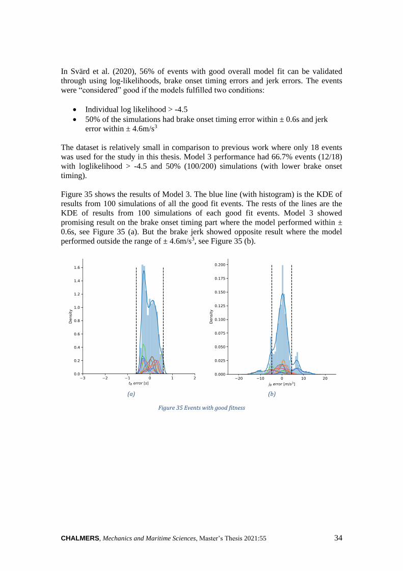
CHALMERS, Mechanics and Maritime Sciences, Master’s Thesis 2021:55 34
In Svärd et al. (2020), 56% of events with good overall model fit can be validated
through using log-likelihoods, brake onset timing errors and jerk errors. The events
were “considered” good if the models fulfilled two conditions:
• Individual log likelihood > -4.5
• 50% of the simulations had brake onset timing error within ± 0.6s and jerk
error within ± 4.6m/s3
The dataset is relatively small in comparison to previous work where only 18 events
was used for the study in this thesis. Model 3 performance had 66.7% events (12/18)
with loglikelihood > -4.5 and 50% (100/200) simulations (with lower brake onset
timing).
Figure 35 shows the results of Model 3. The blue line (with histogram) is the KDE of
results from 100 simulations of all the good fit events. The rests of the lines are the
KDE of results from 100 simulations of each good fit events. Model 3 showed
promising result on the brake onset timing part where the model performed within ±
0.6s, see Figure 35 (a). But the brake jerk showed opposite result where the model
performed outside the range of ± 4.6m/s3, see Figure 35 (b).
(a)
(b)
Figure 35 Events with good fitness

CHALMERS, Mechanics and Maritime Sciences, Master’s Thesis 2021:55 35
4 Discussions
This research aims to develop a driver model of driver brake responses in cut-in
scenario and to fit parameters to and compare the driver model response in computer
simulations with the human driver response from the original cut-in events,
reconstructed from videos of near-crashes in the SHRP2 naturalistic driving study. Four
different computational models were developed, based on an existing rear-end
accumulation driver model in Svärd et al. (2017, 2020). The differences between those
models and the original rear-end model was the calculation of the perceptual input 𝑃(𝑡). Models 1, 2 and 3 were implemented in the virtual simulation framework used (which
use the tool esmini and Python). The model parameters were optimized using Particle
Swarm Optimization (PSO) to fit the model to the driver break onset timing and break
jerk in a set of near-crashes extracted from the SHRP2 naturalistic driving study
(Virginia Tech Transportation Institute, 2020). Model 4 was proposed but never tested,
due to limited project time (therefore it was left for future investigation).
Models 1, 2 and 3 were using different perceptual input based on if the vehicle to cut
in had entered the ego vehicle lane or not (before/after POV-in-lane). Before POV-in-
lane denotes that the POV is completely outside the EGO vehicle's lane, whereas after
POV-in-lane denotes that the POV has reached the lane marking or is in the same lane
as the EGO vehicle, see Figure 13. In Model 1, 𝑃(𝑡) was set to zero before POV-in-
lane. It thus only started to accumulate looming error after POV-in-lane, and 𝑃(𝑡) after
POV-in-lane was calculated with looming using full vehicle angle. Model 2 and 3 used
the same 𝑃(𝑡) calculation as Model 1 for the after POV-in-lane condition, with
additional 𝑃(𝑡) calculations performed before POV-in-lane. Before POV-in-lane, 𝑃(𝑡) in Model 2 was calculated using inverse time to lane crossing (TLC) while also taking
longitudinal range into account. In Model 3, two angles were investigated, the full
vehicle angle and the angle between the POV's corner and the longitudinal direction.
According to the patterns of those two angles in the cut-in scenario, a mathematical
equation was created to calculate 𝑃(𝑡). The optimization process was divided into
training, one training with noise and one training without noise. Models with the best
performance were proceeded training with noise and Model 3 was selected for this part.
The training with noise was performed with 𝜎 = 0 to minimize the least mean square
error of break onset timing and jerk.
4.1 Interpretation of results
Given the method described above, we interpret the results as follows. In section 4.1.1,
the results of different models are interpreted and compared. Section 4.1.2 discuss
possible reasons why the driver model does not fully capture the driver's response
behaviour.
4.1.1 Compare the models
From the training without noise result, the values of accumulation gain K
were very high (got saturated to the maximum of the chosen range) due to P(t) being
set to zero before POV-in-lane and consequently causing very high activity level when
the POV enters the EGO lane at the last moment (when looming already is very high),
resulting in the driver having to brake harshly to avoid collision. The driver model
brake response was delayed 1-1.5 second compared to the real driver brake
responses. Model 1 consequently performance quite poorly, with the responses all

CHALMERS, Mechanics and Maritime Sciences, Master’s Thesis 2021:55 36
being very large. This was expected because in a real-case scenario, the driver will
typically (if he/she is attentive) already act before the POV enters the lane, depending
on the situation.
Model 2 had better performance compared to model 1. Adding the additional predictor
of inverse of time to lane crossing, the driver did have a better braking response and
more “smooth” braking. Model 2 accumulate the perceptual input related to the lateral
and longitudinal distance of the POV and EGO, which is a component that we
considered having potential to mimic driver’s judgement about if the situation is critical
or not. This additional predictor did improve Model 2 overall performance, compared
to Model 1, because the driver Model 2 can act before POV-in-lane, which resembles
a real driver response, which Model 1 did not. However, the results were still
substantially different from that of the original events (the real driver braking response),
with a 0.8-0.9 second delay. Due to the Kalman filter being initiated after POV-in-lane,
the value of 𝑃(𝑡) dropped to zero at POV-in-lane timing, which resulted in a
discontinuity in activity. The solution could be starting the Kalman filter earlier to
provide enough time for the filter to converge. Another reason for the poor model
performance could be that directly adding a linear scaling of longitudinal range on the
denominator with inverse time to lane crossing does not adequately capture how a
human driver response.
The performance of Model 3 was slightly better than Model 2 with only an average of
0.5 second delay in braking response, compared to the real drivers. The brake jerk error
between the driver model output and human driver response was large. In Model 3, the
value of 𝑃(𝑡) was not ‘smooth’ at POV-in-lane timing because the calculation
equations were different before and after the POV-in-lane, and it might result in a large
change in activity level. The sudden change in activity at POV-in-lane timing was
caused by using different calculation equations before and after POV-in-lane, rather
than a sudden change in situation (e.g., urgent braking/accelerating of POV). It is
difficult to smooth it by scaling the first part to fit the magnitude of the second part.
Assigning a scaling factor to each time step is difficult because it is impossible to
predict when the POV will reach the lane mark. One possible solution that could help
in this situation is to shift the 𝑃𝑝(𝑡) by the same amount as the change in 𝑃(𝑡), to ensure
that ℇ(𝑡) does not change when changing equations. ℇ(𝑡) is the error between 𝑃𝑝(𝑡)
and 𝑃(𝑡), which was accumulated in each timestep. As a result, there will still be a
discontinuity in 𝑃(𝑡), but it will have little effect on the activity.
To estimate the model’s performance with noise, the three models (with optimal
parameters from training without noise) were tested with noise 𝜎 = 0.97 (from optimal
value of base model in Svärd et al. (2020)). For each model, Monte Carlo simulations
were performed, and the total loglikelihood and AIC of each model were calculated to
assess the model performance with noise. Model 3 provided the highest total log
likelihood and lowest AIC. Hence Model 3 had the best performance after training
without noise and we chose to run optimization with noise for this model.
After training Model 3 with noise, the total log likelihood for both the training and the
test sets were slightly better than training without noise. The final average log
likelihood of the training set was -4.093 and the final average log likelihood of the test
set was -3.29. The brake onset timing from 200 Monte Carlo simulations were
approximately within ±1 second from human driver for 8/12 events in training set and
4/6 events in test set. All events in training set had brake onset timing errors within ±2

CHALMERS, Mechanics and Maritime Sciences, Master’s Thesis 2021:55 37
seconds and all events in test set had brake onset timing errors ± 1.5 seconds. The
model performance on jerk was even poorer. The jerk errors were within ± 20 m/s3 for
10/12 events in training set. The jerk errors of some Monte Carlo simulations from the
remaining two events in training set were slightly above 20 m/s3. The jerk errors of 5/6
events in test set were within ± 15 m/s3, and the jerk errors were slightly above 15 m/s3
for the remaining event in test set. In summary, even if Model 3 was the best model,
the overall performance of Model 3 was simply not good enough for its intended use.
Compared to the reduced-complexity rear-end model in Svärd et al. (2020), Model 3
had the similar performance on break onset timing, while the jerk errors in Model 3
were larger than the rear-end model in Svärd et al. (2020). As mentioned in result
section, we compare the model performance with Svärd et al. (2020) in terms of log
likelihood. However, it is really hard to tell if the model is good comparing to rear end
model in Svärd et al. (2020) , because it is not obvious which method should be used
to compare models.
4.1.2 Likely reasons to why the driver model does not fully capture
the driver's behaviour
There are many possible reasons why the driver models did not capture the behaviours
of the real-world (original event) drivers. Data quality, the parameter fitting, and/or the
predictors and components of the driver model are the most likely suspects. In the
following we discuss these potential issues in turn.
Data quality
There were events with low video resolution and annotators have to sometime assume
the POV current position, which can lead to an “incorrect” trajectory. When the
longitudinal range is large, the uncertainty of the lateral range result from the annotation
tool is high, resulting in poor data quality. Even if the data was manually modified,
good data quality cannot be guaranteed because the modified ranges were measured
from the front view video with eyes-only-based adjustments.
Parameter fitting (the optimization process)
In Model 1 and 2, the value of accumulation gain 𝐾 was saturated to the maximum of
the selected range, while the value of the sum of non-looming evidence for or against
braking 𝑀 was saturated to the minimum of the selected range. To reach the threshold
faster, both Model 1 and Model 2 tended to have a higher change rate of activity.
Because the driver model in Model 1 does not react before POV-in-lane, and activity
in Model 2 drops to zero at POV-in-lane timing, the break onset timing errors may
become smaller as the change rate of activity increases. If the boundaries were wider,
the value of 𝐾 would increase and the value of 𝑀 will decrease, resulting in a quicker
change in activity (as Equation (1)). However, it will not substantially improve model
performance. Regardless of how quickly activity changes, Model 1 will not react earlier
than POV-in-lane timing. To achieve a better and more ‘stable' performance in Model
2, it is preferable to fix the discontinuity problem in 𝑃(𝑡) rather than having a higher
activity change rate. The optimization process was divided into training without noise
using least mean square and training with noise using maximum log likelihood. To save
computing time, the parameter boundaries of training with noise were located around
optimal parameter from training without noise with a narrow spread. As a result, the
actual global optimal may be outside the boundary.
The predictors and components of the driver model

CHALMERS, Mechanics and Maritime Sciences, Master’s Thesis 2021:55 38
There are large variabilities both with respect to crash causation and driver responses
in real world. Also, the driver models did not capture all the important information from
the drivers (e.g., glance behaviour; however, we did remove the SHRP2 events where
distraction was stated as a contributing factor) and the environment (e.g. the POV turn
signal, the presence of other road users, etc.), which consequently could also be a reason
of poor performance. It may also be that we missed to include some perceptual cue(s),
or its derivative, that drivers use when deciding if a car warrants a braking or not.
4.2 Methodological choices
Virtual simulations are widely used in assessment of AS and ADAS functions, and there
are numerous virtual simulation tools available, including OpenPass, Virtual Test Drive
(VTD) and Esmini. OpenPass provides a free access framework for a reliable method
of completing function effectiveness analyses (Invisiblefarm s.r.l., 2014). In Rösener et
al. (2017), simulations of various scenarios were performed using OpenPass to access
the safety impacts of ADAS functions from European research project AdaptIVe. VTD
(Hexagon AB, 2021) is a powerful rail or road based simulation toolchain that can be
use in Software in the Loop (SiL), Driver in the Loop (DiL), Vehicle in the Loop (ViL)
Hardware in the Loop (HiL). Laschinsky et al. (2010) tested the influence of an Active
Safety Light on the reaction of the driver using Virtual Test Drive with ViL. We had
access to VTD for this thesis, but we chose not to use it because the VTD learning
process (step-in effort to run a complete simulations) was much more difficult/time-
consuming than Esmini's, and we also had our support (supervisor etc) only just started
using VTD. Esmini is a free and open source virtual simulator and was initially
developed from the Swedish collaborative research project Simulation Scenarios. It is
simple to integrate it into custom applications by linking the inclusive shared library to
whatever software you want to use (Emil Knabe, 2021). Volvo Cars provided scripts
for integrating Esmini with Python. Another reason for selecting Esmini was that there,
when we started the thesis, was an ongoing project (L3Pilot, 2021) that used Esmini
for cut-in safety benefit assessment – which was a perfect fit to our thesis topic. A
description of its use in L3Pilot can be found in the L3Pilot Deliverable D7.4 Impact
Evaluation Results, which is currently (at the time of writing this thesis) being drafted.
Estimating derivatives from noisy signals was required in the driver models in this
thesis. Kalman filter has excellent performance in dealing with signals that contains
Gaussian noise and was therefore chosen for this part. Shaowei & Shanming (2012)
used a Kalman filter with adaptive noise variance to estimate motor velocity, with
results that were very close to the actual values. Moving average filters are also
commonly used to estimate derivatives from noisy signals, and they are conceptually
and practically simple to understand and implement. Kalman Filter is a more accurate
and smoothing prediction algorithm comparing to the moving average filter, because it
is adaptive and it takes estimation errors from different sources (and processes) into
account, and tries to adjust the predicted values based on what it learned in the previous
stage (CQG Integrated Client, 2021). The estimation results from an average moving
filter will lag behind the true state. It will be more accurate if a larger time interval is
used, but the lagging will be more severe.
In terms of model parameter fitting, the models in this thesis are complex, with a large
number of parameters, which means using random search and grid search would be
inefficient (Liashchynskyi & Liashchynskyi, 2019). Furthermore, because it is not a
differentiable problem, any algorithm involving gradient descent was out of the

CHALMERS, Mechanics and Maritime Sciences, Master’s Thesis 2021:55 39
question. We used PSO as the optimization technique for fitting model parameters.
There are other Evolutionary Algorithms that are similar, such as Genetic Algorithm
(GA) and Differential Evolution (DE). DE and PSO are better suited to continuous
optimization, whereas GA is more suitable for discrete optimization
(Kachitvichyanukul, 2012). In parameter fitting of the accumulation driver model, DE
and PSO are preferable to GA because the parameters can be set to any value within
the boundary. It was also mentioned in Kachitvichyanukul (2012) that, comparing to
DE , the global optimal of PSO in each iteration has a dominant influence over the
whole swarm, which enables solution improvement with shorter time (than DE).
However, diversification of DE is better than PSO because the best solution in the
population has no influence on the other solutions in the population. In Zgonnikov et
al. (2020), an accumulation driver model was developed for predicting whether the
drivers will make a left turn across path of an oncoming car. The model was fitted into
data in terms of probability of turn decisions and the response time for the “turn”
decisions. DE was chosen using cost function of weighted least sum score. While in
Svärd et al. (2020) and this thesis, the calculation of cost (maximum log likelihood) of
each parameter set requires a large number of repeating simulations to generate a 2D
distribution of break onset timing and jerk, which means a high computing time. As a
result, PSO may be a better solution than DE.
4.3 Limitations and Future work
The SHRP2 dataset that were available to us contained 209 cut-in events with forward
facing video, but after we applied the inclusion and exclusion criteria only 18 events
remained (Section 2.1). Removing 191 (91.3%) events and only having 18 events “to
work with” was naturally a major limitation. However, we believe that our focus on the
methodological aspects of the modelling, and the design of relevant predictors still
provided a good thesis and learning opportunities, and results that can be a stepping
stone for future research. One solution to improve the data quality is either use a
different data extraction tool or improve video annotation tool, or a different dataset, if
available.
Initially, there was supposed to be four different driver models, but due to limited time,
one driver (Model 4) was excluded in this study. Model 4 (proposed, not implemented)
is more based on human peripheral vision and how driver utilize peripheral vision to
perform different driving task. This includes object movement, road signs, monitor
traffic, stay within the lane etc. (Edmund Hunter, n.d.). The POV will mostly be inside
the EGO peripheral vision during cut-ins but if the POV is outside “center of vision”,
the driver may react slower to cut-ins. First the EGO driver needs to identify the object
with his/her the peripheral vision, then move the eyes to it, then make a decision based
on the situation, and, finally initiate a brake response, if needed. All this together may
add to the brake respond “delay”. However, this is likely to not be an issue if the EGO
driver is already looking at the POV at the start of cut-in event. Consequently, glance
behavior data for each event is needed in the modelling to enable the consideration of
peripheral versus foveal vision in the model. Specifically, Model 4 utilize human
peripheral vision in traffic as a constraint. Studies show that peripheral vision will
change depending on speed, and that may have in impact on how peripheral vision
should be included in the model (Shbeeb, 2016). Model 4 could potentially have
increased the performance of the model, but was never implemented and fitted to the
data. The Wolfe et al. (2017) report demonstrated this peripheral vision in traffic with
live camera, to get a clearer picture how this looks in real traffic with center of vision

CHALMERS, Mechanics and Maritime Sciences, Master’s Thesis 2021:55 40
(Figure 3 on p. 321 in Wolfe et al. (2017)). When the driver is changing their focus area
(center of vision), everything outside the focus area becomes blurry. In the picture
(Figure 3 p. 321 in Wolfe et al. (2017) ), a red circle is where driver is currently looking.
When the driver is shifting their center of vision from b to c and c to d, everything
outside the red circle is blurry. This is an interesting phenomenon to investigate for
future cut-in driver models, as it may substantially affect the perception and response
in cut-in situations.
We started the work using an already existing dataset, that late in the thesis work was
found to have errors in the POV lateral position. Before we found this and addressed it
(through semi-manual correction) we conducted several analyses on the data that we
did not have time to redo on the new dataset. For example, on the original dataset we
performed random selection of event and K-Fold cross-validation to analyse the
sensitivity of event selection and data variability. K-Fold cross-validation is a popular
method in machine learning world to estimate the performance of models and selection
of models (Jung, 2018). Such analysis requires a lot of computing time and therefor
was left for future investigation for the new (corrected) dataset. The initial plan was
also to use this training process to reduce number of trained parameters. The remaining
18 events was divided into two different set, 12 events for training and 6 for
test. This training data is extremely small for such complex driver model with 8 free
parameters. The size of training data might not be large enough to optimize the
parameters using PSO. As for the future, increasing the training dataset, reducing
complexity of the model and reduce simulation time will allow more time for trial and
error, improve the driver model performance. Because optimisation with noise required
a high computing time, it was only done once with relatively low interactions and a
narrow parameter boundary. The true optimal value could lay outside of the boundary.
Finding a better way to define parameter boundaries could aid in the resolution of this
issue. Another option is to reduce the model's complexity. When the model has a small
number of parameters, fewer interactions and less computation time are required.
The complexity and limited time available for this thesis were major factors in how
what we pursued and what we could complete. For example, driver off-road glance
behaviour was not considered in this thesis, although it is an important part. Driver
distraction is a normal behaviour in traffic and can greatly deteriorates driving
performance (Donmez et al., 2010). Future studies should investigate the role of the
driver’s peripheral vison versus fovia vision on the cut-in vehicle. As mentioned before,
the discontinuity of 𝑃(𝑡) at POV-in-lane timing, caused by the changing of calculation
equations, should be studied in future work, with the aim to create a continues
accumulation function. Finally, this work is one step in the direction of driver response
models for cut-in scenarios. With further development we hope that it can be used as
part of virtual safety benefit assessment of active safety systems and possibly for
vehicles with higher levels of automation.

CHALMERS, Mechanics and Maritime Sciences, Master’s Thesis 2021:55 41
5 Conclusion
This thesis extended an existing rear-end accumulation driver model to a cut-in driver
model to predict the braking of the driver. This study showed it is possible to use the
video annotation tool to extract necessary information from naturalistic driving data
and later reconstruct near-crash events in virtual simulation. Three model proposals
with different perceptual input calculations were introduced and implemented in virtual
simulation. The model’s parameter was optimized with the stochastic optimization
method PSO, to fit the parameters to real-world naturalistic near-crash data. The
optimization process was divided into two separate parts, one without noise and second
one with noise to save more computing time. Model 1 was only activated after POV-
in-lane and it had the worst performance (late response), which indicated that in real
world, the driver usually response before the POV reached the lane mark. The best
performing model (Model 3) were selected for training with noise and had more
parameters (8 in total) compared to rear-end driver model from previous work. This
indicate that sometimes it is necessary to increase the model complexity in order to
capture more perceptual cues from drivers. The validation method of the models was
based on previous work on rear-end driver model.
The Model 3 had a better performance than Model 1 and 2 but it still not good enough.
The models did not capture all the necessary mechanisms, such as glance behaviour or
distraction was excluded in this study. The model needs further improvement, both by
reducing the complexity of the model (reduce computing time) and adding additional
relevant parameters that can capture more information about the driver (improve
accuracy). However, Model 3 did perform well on brake onset timing but showed
weaker jerk compared to real drivers in some of the simulations. With further
development, the driver model could be used in virtual simulations to do safety
assessment of active safety or other vehicle automation functions. A future validated
driver model could mimic the possible reactions from a driver in a cut-in situation, and,
consequently being used to generate baseline events and as part of warning strategies
in cut-in conflicts. Including some variability in the parameters (including noise) can
make the situation is a little bit different (but capturing within and between driver
variabilities), making the assessment results more robust.

CHALMERS, Mechanics and Maritime Sciences, Master’s Thesis 2021:55 42
6 References
Almeida, B. S. G. de, & Leite, V. C. (2021). Particle Swarm Optimization: A
Powerful Technique for Solving Engineering Problems. 2019-12-03.
https://www.intechopen.com/books/swarm-intelligence-recent-advances-new-
perspectives-and-applications/particle-swarm-optimization-a-powerful-
technique-for-solving-engineering-problems
Bärgman, J. (2019). Signal processing assignment from Vehicle and Traffic Safety.
Chalmers University of Technology.
Benderius, O. (2012). Driver modeling: data collection, model analysis, and
optimization. Thesis for Licentiate of Engineering, 2012:11, 58.
http://publications.lib.chalmers.se/records/fulltext/157634.pdf%0Ahttps://trid.trb.
org/view/1367670
Chovan, J. D., Tijerina, L., Alexander, G., & Hendricks, D. L. (1994). Examination of
Lane Change Crashes and Potential IVHS Countermeasures. Report No. DOT HS
808 071, U.S. Department of Transportation, March, 50.
CQG Integrated Client. (2021). Basic Studies - Kalman Filter. CQG Integrated Client.
Din, A. H. S. El, Takkoush, M., Pettersson, N., & ... (2020). Variables extraction and
trajectory reconstruction for modelling driver behaviour.
https://odr.chalmers.se/handle/20.500.12380/300751
Donmez, B., Boyle, L. N., & Lee, J. D. (2010). Differences in off-road glances:
Effects on young drivers’ performance. Journal of Transportation Engineering,
136(5), 403–409. https://doi.org/10.1061/(ASCE)TE.1943-5436.0000068
Edmund Hunter. (n.d.). Module 3: Topics 1-3 Vision and Driving. 2016 IEEE 19th
International Conference on Intelligent Transportation Systems (ITSC).
https://slideplayer.com/slide/10872053/
Emil Knabe. (2021). Environment Simulator Minimalistic (esmini). 2021.
https://github.com/esmini
Gordon, T., & Srinivasan, K. (2014). Modeling human lane keeping control in
highway driving with validation by naturalistic data. Conference Proceedings -
IEEE International Conference on Systems, Man and Cybernetics, 2014-
Janua(January), 2507–2512. https://doi.org/10.1109/smc.2014.6974303
Helmer, T., Wang, L., Kompass, K., & Kates, R. (2015). Safety Performance
Assessment of Assisted and Automated Driving by Virtual Experiments:
Stochastic Microscopic Traffic Simulation as Knowledge Synthesis. 2015 IEEE
18th International Conference on Intelligent Transportation Systems, 2019–
2023. https://doi.org/10.1109/ITSC.2015.327
Hexagon AB. (2021). Virtual Test Drive. 2021.
https://www.mscsoftware.com/product/virtual-test-drive
Invisiblefarm s.r.l. (2021). OpenPass for open system of controlled access. 2014.
http://www.openpass.it/
Jung, Y. (2018). Multiple predicting K-fold cross-validation for model selection.
Journal of Nonparametric Statistics, 30(1), 197–215.
https://doi.org/10.1080/10485252.2017.1404598
Kachitvichyanukul, V. (2012). Comparison of Three Evolutionary Algorithms: GA,
PSO, and DE. Industrial Engineering and Management Systems, 11, 215–223.
L3Pilot. (2021). L3Pilot. L3Pilot.
Laschinsky, Y., von Neumann-Cosel, K., Gonter, M., Wegwerth, C., Dubitzky, R., &
Knoll, A. (2010). Evaluation of an Active Safety Light using Virtual Test Drive
within Vehicle in the Loop. 2010 IEEE International Conference on Industrial
Technology, 1112–1119. https://doi.org/10.1109/ICIT.2010.5472583

CHALMERS, Mechanics and Maritime Sciences, Master’s Thesis 2021:55 43
Liashchynskyi, P., & Liashchynskyi, P. (2019). Grid Search, Random Search, Genetic
Algorithm: A Big Comparison for NAS.
Markkula, G. (2014). Modeling driver control behavior in both routine and near-
accident driving. Proceedings of the Human Factors and Ergonomics Society,
2014-Janua, 879–883. https://doi.org/10.1177/1541931214581185
Markkula, G., Benderius, O., Wolff, K., & Wahde, M. (2012). A review of near-
collision driver behavior models. Human Factors, 54(6), 1117–1143.
https://doi.org/10.1177/0018720812448474
Page, Y., Fahrenkrog, F., Fiorentino, A., Gwehenberger, J., Helmer, T., Lindman, M.,
Camp, O., Rooij, L. V, Puch, S., Fränzle, M., Sander, U., & Wimmer, P. (2015).
A comprehensive and harmonized method for assessing the effectiveness of
advanced driver assistance systems by virtual simulation: The P.E.A.R.S.
QUADRAE. (2021). QUADRAE. 2021-03-31.
https://www.saferresearch.com/projects/quadrae
Rösener, C., Sauerbier, J., Zlocki, A., Fahrenkrog, F., Wang, L., Varhelyi, A., Gelder,
E., Breunig, S., Tango, F., & Lanati, J. (2017). A Comprehensive Evaluation
Approach for Highly Automated Driving.
Shams El Din, A. H. (2020a). Statistical modelling of critical cut-ins for the
evaluation of autonomous vehicles and advanced driver assistance systems.
https://hdl.handle.net/20.500.12380/301054
Shams El Din, A. H. (2020b). Statistical modelling of critical cut-ins for the
evaluation of autonomous vehicles and advanced driver assistance systems.
Shaowei, W., & Shanming, W. (2012). Velocity and acceleration computations by
single-dimensional Kalman filter with adaptive noise variance. Przeglad
Elektrotechniczny, 88(2), 283–287.
Shbeeb, D. L. (2016). Human component and vehicle in transportation. 2016-01-30.
https://www.slideshare.net/hronaldo10/driver-vehicle-transportation-
engineering-drlina-
shbeeb?fbclid=IwAR3uQimT1K00a65CNugQtPEtTr9wDLHmiN3QUlOMQtp3
z4XQSrFaSLJchZc
Svärd, M., Markkula, G., Bärgman, J., & Victor, T. (2020). Computational modeling
of driver pre-crash brake response, with and without off-road glances:
Parameterization using real-world crashes and near-crashes.
https://doi.org/10.31234/osf.io/6nkgv
Svärd, M., Markkula, G., Engström, J., Granum, F., & Bärgman, J. (2017). A
quantitative driver model of pre-crash brake onset and control. Proceedings of
the Human Factors and Ergonomics Society Annual Meeting, 61(1), 339–343.
https://doi.org/10.1177/1541931213601565
Virginia Tech Transportation Institute. (n.d.). DATA REDUCTION. 2021.
https://www.vtti.vt.edu/facilities/data-reduction.html
Virginia Tech Transportation Institute. (2021). InSight Data Access Website SHRP2
Naturalistic Driving Study. 2020. https://insight.shrp2nds.us/
Wolfe, B., Dobres, J., Rosenholtz, R., & Reimer, B. (2017). More than the Useful
Field: Considering peripheral vision in driving. Applied Ergonomics, 65, 316–
325. https://doi.org/10.1016/j.apergo.2017.07.009
Zgonnikov, A., Abbink, D., & Markkula, G. (2020). Should I stay or should I go?
Evidence accumulation drives decision making in human drivers.
https://doi.org/10.31234/osf.io/p8dxn

CHALMERS, Mechanics and Maritime Sciences, Master’s Thesis 2021:55 44
Appendix
Result of Model 3 – training without noise 1st run – training set
Figure 36 Event1
Figure 37 Event2
Figure 38 Event3
Figure 39 Event4
Figure 40 Event5
Figure 41 Event6

CHALMERS, Mechanics and Maritime Sciences, Master’s Thesis 2021:55 45
Figure 42 Event7
Figure 43 Event8
Figure 44 Event9
Figure 45 Event10
Figure 46 Event11
Figure 47 Event12

CHALMERS, Mechanics and Maritime Sciences, Master’s Thesis 2021:55 46
Result of Model 3 – training without noise 1st run – test set
Figure 48 Event13 Figure 49 Event14
Figure 50 Event15
Figure 51 Event16
Figure 52 Event17
Figure 53 Event18

CHALMERS, Mechanics and Maritime Sciences, Master’s Thesis 2021:55 47
Result of Model 3 – training with noise – training set
Figure 54 Event1
Figure 55 Event2
Figure 56 Event3
Figure 57 Event4
Figure 58 Event5
Figure 59 Event6

CHALMERS, Mechanics and Maritime Sciences, Master’s Thesis 2021:55 48
Figure 60 Event7
Figure 61 Event8
Figure 62 Event9
Figure 63 Event10
Figure 64 Event11
Figure 65 Event12

Result of Model 3 – training with noise – test set
Figure 66 Event13
Figure 67 Event14
Figure 68 Event15
Figure 69 Event16
Figure 70 Event17
Figure 71 Event18

DEPARTMENT OF MECHANICS AND
MARITIME SCIENCE CHALMERS
UNIVERSITY OF TECHNOLOGY
Gothenburg, Sweden 2021
www.chalmers.se