Driver Drowsiness Detection based on Non-intrusive Metrics Considering 1

Individual Specifics 2

3

Xuesong Wang, PhD 4

Professor 5

School of Transportation Engineering, 6

Tongji University 7

4800 Cao’an Road, Jiading District 8

Shanghai, 201804, China 9

Phone: +86-21-69583946 10

Fax: +86-21-69582897 11

Email: wangxs@tongji.edu.cn 12 13

Chuan Xu* 14

PhD student 15

School of Transportation Engineering 16

Tongji University 17

Room 338, Building of School of Transportation Engineering 18

4800 Cao’an Road, Shanghai, 201804, P. R. of China 19

Tel: +86 15216706076 20

Email: xuchuan7@gmail.com 21

(Corresponding Author) 22

23

Xiaohong Chen, PhD 24

Professor 25

School of Transportation Engineering 26

Tongji University 27

4800 Cao’an Road, Shanghai, 201804, P. R. of China 28

Tel) +86-21-65989270 Fax) +86-21-65982897 29

Email: chenxh@tongji.edu.cn 30

31

Word Count: 4732 (Text) +6 Figures+3 Tables=6982words 32

33

July 2014 34

35

36

Submitted for Presentation at the TRB Annual Meeting, and Publication in the Journal of 37

the Transportation Research Board38

1

1

ABSTRACT 2

Drowsy driving is a serious highway safety problem. If drivers could be warned before 3

they became too drowsy to drive safely, some of these crashes could be prevented. 4

Being able to reliably detect drowsiness depends on the presentation of timely warnings 5

of drowsiness. To date, the effectiveness of drowsiness detection methods has been 6

limited by their failure to consider individual differences. The present study sought to 7

develop a drowsiness detection model that accommodates the varying effects of 8

drowsiness on individual driving performance. Nineteen driving behavior variables and 9

four eye feature variables were measured as participants drove a fixed road course in a 10

high fidelity motion-based driving simulator after having worked an 8-hour night shift. 11

During the test, participants were asked to report their drowsiness level using the 12

Karolinska Sleepiness Scale (KSS) at the midpoint of each of the six rounds through 13

the road course. A multilevel Ordered Logit model (MOL), an Ordered Logit model 14

(OL), and an Artificial Neural Network model (ANN) were used to determine 15

drowsiness. The MOL had the highest drowsiness detection accuracy, and this finding 16

shows that consideration of individual differences improves the models’ ability to 17

detect drowsiness. According to the results of the models, percentage of eyelid closure, 18

average pupil diameter, standard deviation of lateral position and steering wheel 19

reversals were most important in the 23 variables. 20

21 Keywords: Drowsiness Detection, Multilevel Ordered Logit Model, Non-Intrusive, 22

Driving Behavior, Eye Feature, Driving Simulator 23

24

2

1 INTRODUCTION 1

2

Drowsy driving is a serious threat to road safety. In 2009, over 800 fatalities and 30,000 3

injuries from car crashes were attributed to drowsy driving in the United States (1). In 4

Europe, an estimated 20% of traffic crashes are caused by drowsy driving (2). The 5

problem seems more serious in China where, in 2007, 1768 fatalities were attributed to 6

drowsy driving (3). Considering that as of 2012, China had over 85,000 kilometers of 7

expressways (4), and the annual growth in kilometers exceeded 14% during 2002-2011, 8

the problem requires immediate attention. A recent study using a naturalistic driving 9

method, estimated the increase in crash risk associated with drowsy driving to be four 10

to six times greater than when driving while alert (5). Besides increasing crash risk, 11

drowsy driving crashes are often more severe than other crashes because they 12

frequently occur on high speed expressways, and are frequently run-off-the-road 13

crashes with no braking prior to impact. 14

Unlike drinking and driving, drowsy driving does not provide an objective 15

measure of its occurrence, and therefore enforcement cannot be used to counter this 16

problem (6). An alternative would be to notify the driver if he becomes too drowsy to 17

drive safely. This requires the reliable detection of drowsy driving—a problem that has 18

been extensively researched. Based on the type of data used, drowsiness detection can 19

be conveniently separated into the two categories of intrusive and non-intrusive 20

methods. Intrusive methods, such electroencephalograms (EEGs) (7) or 21

electrocardiograms (EKGs) (8), show good detection accuracy, however, are limited to 22

the research laboratory. In contrast, methods based on non-intrusive measures detect 23

drowsiness by measuring driving behavior and sometimes eye features, and so are 24

useful for real world driving situations. 25

To date, non-intrusive methods have been less reliable than intrusive methods, 26

partly because individual differences in non-intrusive measures have prevented the 27

identification of the point at which drowsiness impairs driving (9; 10). In the previous 28

research, individual differences of non-intrusive methods were frequently mentioned, 29

for both driving behavior and eye features. For driving behavior, Ingre et al. (9) report 30

the individual difference of standard deviation of lateral position (SDLP), an important 31

driving behavior measure to drowsiness. In this research, for the same drowsiness level, 32

different drivers have different SDLPs. Another study finds the individual difference of 33

driver’s lane departure behavior (11). Thiffault and Bergeron (12) reported the 34

individual difference of the standard deviation of steering wheel movements. Regarding 35

eye features, individual differences of blink duration (9; 13), percentage of eyelid 36

closure (PERCLOS) (14) were also observed in many studies. However, most 37

drowsiness detection methods such as decision trees, logistic regression, Bayesian 38

networks (15), artificial neural networks (8), and support vector machines (16) have not 39

properly handled the problem of differences in the manifestation of drowsiness among 40

individuals. Ignoring such differences reduces the accuracy and reliability of these 41

models, especially for non-intrusive measures. 42

To address and increase the accuracy for drowsiness detection model based on 43

non-intrusive measures, a multilevel logit model was built based on both driving 44

3

behavior measures and eye features, which detect drowsiness by using individual-1

specific criterions. To compare the detection accuracy, two non-individual specific 2

models (i.e., ordered logit model and artificial neural network) were established. All 3

the data in this research is based on a high fidelity driving simulator experiment, in 4

which driving behavior, eye features, and subjective drowsiness were scaled and 5

collected. 6

7

2 METHOD 8

2.1 Participants 9

Sixteen male participants aged 24-40 (mean 32.8, SD, 5.0) with valid Chinese drivers 10

licenses were recruited from students and staff at Tongji University. They were required 11

to be in good health, have no sleep related disorders, and not to have taken any 12

pharmaceuticals within one month prior to entering the study. Subjects who had a 13

history of motion sickness were screened out. All subjects provided written consent and 14

were paid about 200 RMB Yuan, depending on the total time in the laboratory. During 15

the experiment, one subject’s eye movement data was lost because of a technical 16

problem. One subject fell asleep before completing the task, however, his data up to 17

that point was used. 18

19

2.2 Apparatus 20

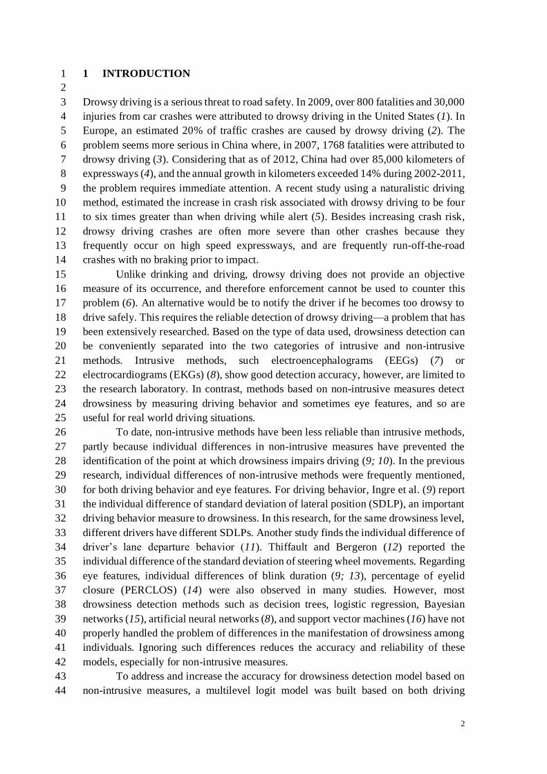
The Tongji University driving simulator is shown in FIGURE 1. This simulator, 21

currently the most advanced in China, incorporates a fully instrumented Renault 22

Megane III vehicle cab in a dome mounted on an 8 degree-of-freedom motion system 23

with an X-Y range of 20 × 5 meters. An immersive 5 projector system provides a front 24

image vi Tongji advanced driving simulator ew of 250° × 40° at 1000 × 1050 resolution 25

refreshed at 60 Hz. LCD monitors provide rear views at the central and side mirror 26

positions. SCANeRTM studio software presented the simulated roadway and controlled 27

a force feedback system that acquired data from the steering wheel, pedals and gear 28

shift lever. 29

30 FIGURE 1 Tongji advanced driving simulator 31

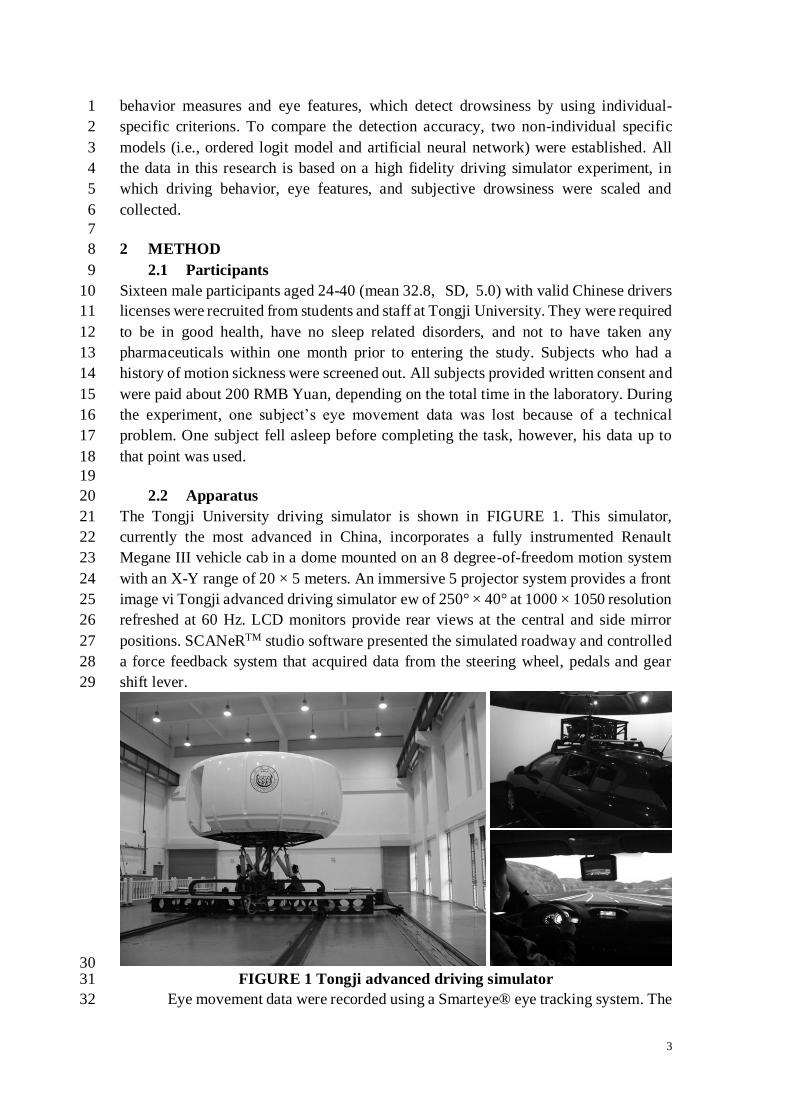
Eye movement data were recorded using a Smarteye® eye tracking system. The 32

4

cameras and interface of this system are shown in FIGURE 2. The system uses four 1

cameras located in the front of the vehicle to record the driver’s eye movements at 60 2

Hz sampling rate. 3

4

5 FIGURE 2 Smarteye® eye tracking system hardware and software interface 6

7

2.3 Procedure 8

2.3.1 Experiment design 9

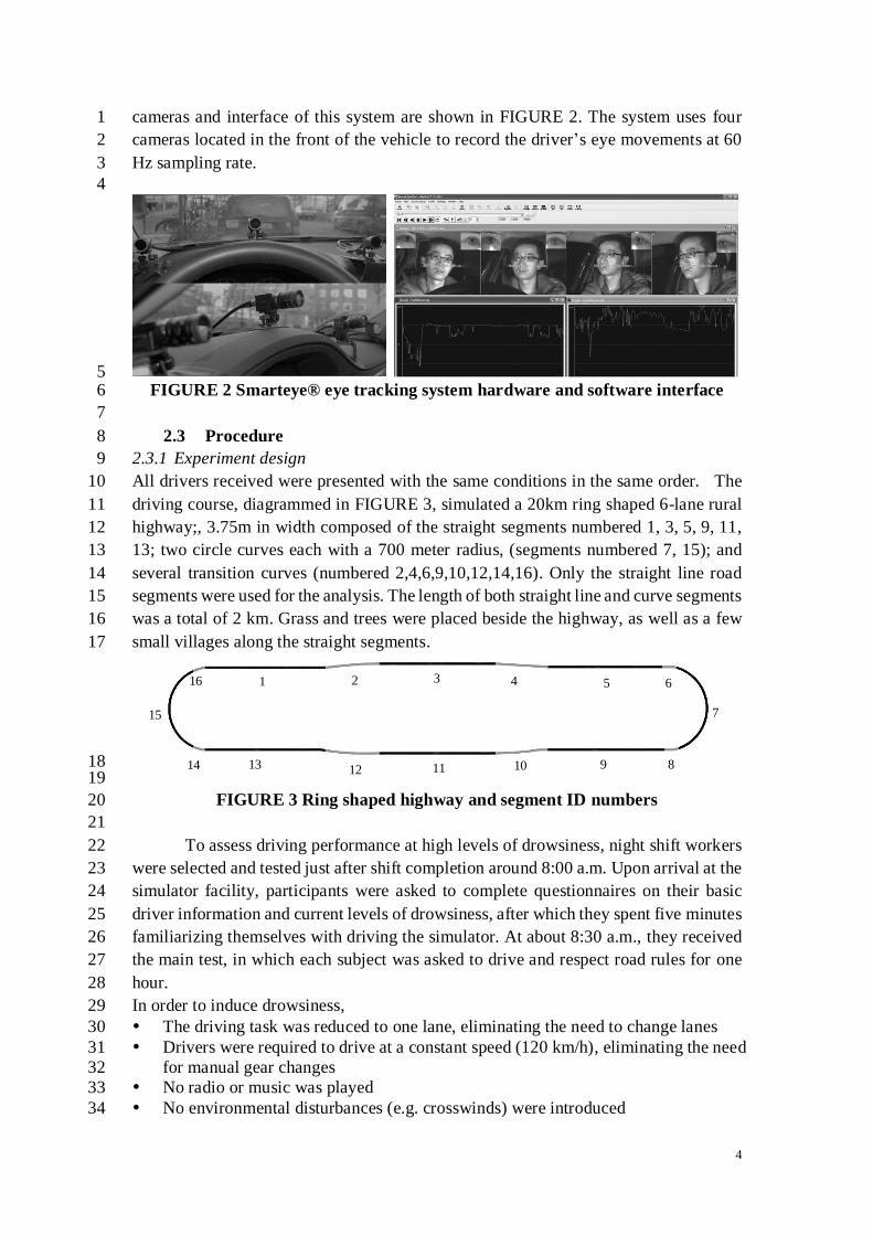
All drivers received were presented with the same conditions in the same order. The 10

driving course, diagrammed in FIGURE 3, simulated a 20km ring shaped 6-lane rural 11

highway;, 3.75m in width composed of the straight segments numbered 1, 3, 5, 9, 11, 12

13; two circle curves each with a 700 meter radius, (segments numbered 7, 15); and 13

several transition curves (numbered 2,4,6,9,10,12,14,16). Only the straight line road 14

segments were used for the analysis. The length of both straight line and curve segments 15

was a total of 2 km. Grass and trees were placed beside the highway, as well as a few 16

small villages along the straight segments. 17

18 19

FIGURE 3 Ring shaped highway and segment ID numbers 20

21

To assess driving performance at high levels of drowsiness, night shift workers 22

were selected and tested just after shift completion around 8:00 a.m. Upon arrival at the 23

simulator facility, participants were asked to complete questionnaires on their basic 24

driver information and current levels of drowsiness, after which they spent five minutes 25

familiarizing themselves with driving the simulator. At about 8:30 a.m., they received 26

the main test, in which each subject was asked to drive and respect road rules for one 27

hour. 28

In order to induce drowsiness, 29

The driving task was reduced to one lane, eliminating the need to change lanes 30

Drivers were required to drive at a constant speed (120 km/h), eliminating the need 31

for manual gear changes 32

No radio or music was played 33

No environmental disturbances (e.g. crosswinds) were introduced 34

16 1 2 3 4 5 6

7

8 9 10 11 12 13 14

15

5

All driving was during daytime periods and no tunnel or weather changes occurred 1

eliminating the need to adjust headlights 2

Only occasional and uneventful traffic was present. 3

After the main test, participants were asked to complete post experiment 4

questionnaires on their levels of drowsiness. 5

6

2.3.2 Measurement of drowsiness—participants’ assessments 7

To track drivers’ drowsiness changes during the one hour driving task, the participants 8

were asked to report their Karolinska Sleepiness Scale (KSS) level at the middle point 9

of pass through the driving course. KSS is on a 9 point ordinal scale, however, it’s not 10

necessary to distinguish all nine levels when using the KSS. It is, however necessary 11

to identify the drowsiness level with a high crash risk. Several studies (15; 17) 12

suggested that serious behavioral and physiological changes do not occur until KSS>=7. 13

In addition, the description of KSS 7 is “sleep, but no effort to keep alert,” but KSS 8, 14

9 are described as “need some or great effort to keep alert.” Therefore, drowsiness in 15

this study is categorized into three levels as follows : 16

Level 1 (DL=1): KSS range from 1 to 6, no drowsiness or low-level of drowsiness; 17

Level 2 (DL=2): KSS is 7, moderate-level of drowsiness; 18

Level 3 (DL=3): KSS range from 8 to 9, high-level of drowsiness. 19

20

2.3.3 Measurement of the effects of drowsiness 21

Vehicle-based signals measuring driving behavior, with 10Hz sample frequency, were 22

obtained from the system, including vehicle speed, lateral position and steering wheel 23

angle. Based on these signals, several drowsiness related behavior indicators were 24

extracted. Eye movement signals including eyelid opening and pupil diameter were also 25

recorded, with 60Hz sample frequency. Using the Smarteye Pro software, eye blink was 26

identified. Eye activity indicators including percentage of eye closure (PERCLOS), 27

average pupil diameter, blink frequency, and average blink duration were calculated. 28

The measures are summarized in TABLE 1 below. 29

30

6

TABLE 1 Driving Behavior and Eye Feature Metrics 1 Metrics Description of the Variables Mean S.D.

Driving Behavior

LP_stdev Standard deviation of lateral position (m) 0.306 0.134

LP_avg Average of lateral position (m) 0.214 0.269

LD_Area Sum of lane departure time-space area (m•s) 1.627 4.207

LD_TArea Sum of lane departure time-space area weighted by

lane crossing time (m•s)

6.129 35.383

LD_Frequency Lane departure frequency 0.660 1.118

LD_Speed Lane departure lateral speed (m/s) 0.046 0.099

LD_Tc Time percentage of lane crossing of the vehicle

center

0.002 0.017

LD_Te Time percentage of lane crossing of the vehicle edge 0.021 0.045

SW_Speed_stdev Standard deviation of steering angular speed

(degree/s)

0.012 0.008

SW_Area_MA Area surrounded by steering angle and its moving

average

0.440 0.257

SWM_Re Steering wheel reversals 190.485 29.522

SW_Range_1 Percentage of steering speed in 0-2.5 degree/s 0.876 0.085

SW_Range_2 Percentage of steering speed in 2.5-5 degree/s 0.077 0.037

SW_Range_3 Percentage of steering speed in 5-7.5 degree/s 0.024 0.020

SW_Range_4 Percentage of steering speed in 7.5-10 degree/s 0.010 0.012

SW_Range_5 Percentage of steering speed exceeding 10 degree/s 0.013 0.024

Speed Average speed (km/h) 117.424 6.650

Speed_stdev Standard deviation of speed (km/h) 2.866 2.860

Speeding_T Time percentage of speed exceeding the limit speed

120 km/h

0.311 0.372

Eye Features

Blink_Frequency Average blink frequency per second 0.504 0.318

Blink_duration Average blink duration (second) 0.402 0.054

PERCLOS Percentage of eyelid closure 0.132 0.099

Pupil Average pupil diameter (mm) 3.807 0.894

2.3.4 Data analysis 2

Using DL as the dependent variable, and the driving behavior and eye feature metrics 3

described in TABLE 1 as the independent variables, three models, individual-specific 4

model multilevel ordered logit model, and two non-individual-specific models, an 5

ordered logit model and neural network model. 6

The data set was divided into a training set and a validation set. The data in the 7

training set was used to build the models, and the data in the validation set was used to 8

test the models. To ensure each of the two data sets contained the data from every 9

subject at every drowsiness level, the training set was generated by randomly selecting 10

70% of the data for each subject at each drowsiness level, and the rest of the data was 11

assigned to the validation set. The individual specific multilevel ordered logit model 12

was established first, and then the non-individual specific ordered logit model and 13

neural network model were constructed using the same variables as the multilevel 14

ordered logit model. 15

Multilevel Ordered Logit Model 16

Multilevel ordered logit models are often presented as cumulative logit models. 17

Suppose an ordered DLij is the drowsiness level for ith subject on the jth road segment. 18

A latent continuous variable DLij* is established as the unobserved measure of DL ij. 19

DLij* is related to DLij by a series of latent thresholds. Differing from the ordered logit 20

7

model, the multilevel model accounts for each subject’s individual performance by 1

using a set of variable thresholds specific to each subject: 𝛾𝑘𝑖 (k=1, 2), see formula (2). 2

3

DL𝑖𝑗 = {

1 𝑖𝑓 𝐷𝐿𝑖𝑗∗ < 𝛾1𝑖

2 𝑖𝑓 𝛾1𝑖 < 𝐷𝐿𝑖𝑗∗ < 𝛾2𝑖

3 𝑖𝑓 𝛾2𝑖 < 𝐷𝐿𝑖𝑗∗

(1)

4

The 𝐷𝐿𝑖𝑗∗ can be written in the same form as the regular linear regression 5

model. 6

𝐷𝐿𝑖𝑗

∗ = 𝜃𝑖𝑗 + 𝜀𝑖𝑗 and 𝜃𝑖𝑗 = ∑ 𝛽𝑝𝑥𝑝𝑖𝑗𝑃𝑝=1 (2)

Where 𝑥𝑝𝑖𝑗 is the explanatory variable for ith subject on jth segment. 𝜀𝑖𝑗 is the 7

disturbance term, which is assumed as a logistic distribution as the cumulative density 8

function. Thus, the cumulative response probabilities of the ordinal DL may be denoted 9

as: 10

𝑃𝑖𝑗(𝑘) = Pr(𝐷𝐿𝑖𝑗∗ ≤ 𝑘) = 𝐹(𝛾𝑘𝑖 − 𝜃𝑖𝑗) =

exp (𝛾𝑘𝑖 − 𝜃𝑖𝑗)

1 + exp (𝛾𝑘𝑖 − 𝜃𝑖𝑗), 𝑘 = 1,2 (3)

11

Logit(𝑃𝑖𝑗(𝑘)) = log [𝑃𝑖𝑗(𝑘)

1 − 𝑃𝑖𝑗(𝑘)] = log [

Pr(𝐷𝐿𝑖𝑗∗ ≤ 𝑘)

Pr(𝐷𝐿𝑖𝑗∗ ≥ 𝑘)

] = 𝛾𝑘𝑖 − 𝜃𝑖𝑗, k = 1,2 (4)

In order to accommodate differences among subjects, the thresholds 𝛾𝑘𝑖 were 12

specified as random effects. 13

𝛾𝑘𝑖 = 𝛾𝑘 + 𝑏𝑖 , k = 1, 2 (5)

Where the intercept 𝛾𝑘 represents a constant component for thresholds for all subjects. 14

A random effect component 𝑏𝑖 is formulated to accommodate the between-subject 15

heterogeneities. 16

An Intra-class Correlation Coefficient (ICC) is normally defined to examine the 17

proportion of specific subject-level variance: 18

ICC =𝜎𝑏

2

𝜎𝑏2 + 𝜎𝑤

2 (6)

Where 𝜎𝑤2 is within group variance and 𝜎𝑏

2 is between group variance. A value of 19

ICC close to zero indicates there is a very small variation between the different subjects, 20

and a model without multilevel structure is adequate for the data. Otherwise, a 21

multilevel model would be preferred. 22

23

(2) Artificial Neural Network Model 24

Artificial Neural Networks (ANN), a popular class of computational intelligence 25

models, have been widely applied to drowsiness detection, partly because of their 26

ability to work with massive amounts of multi-dimensional data, their modeling 27

flexibility, and their generally good predictive ability. 28

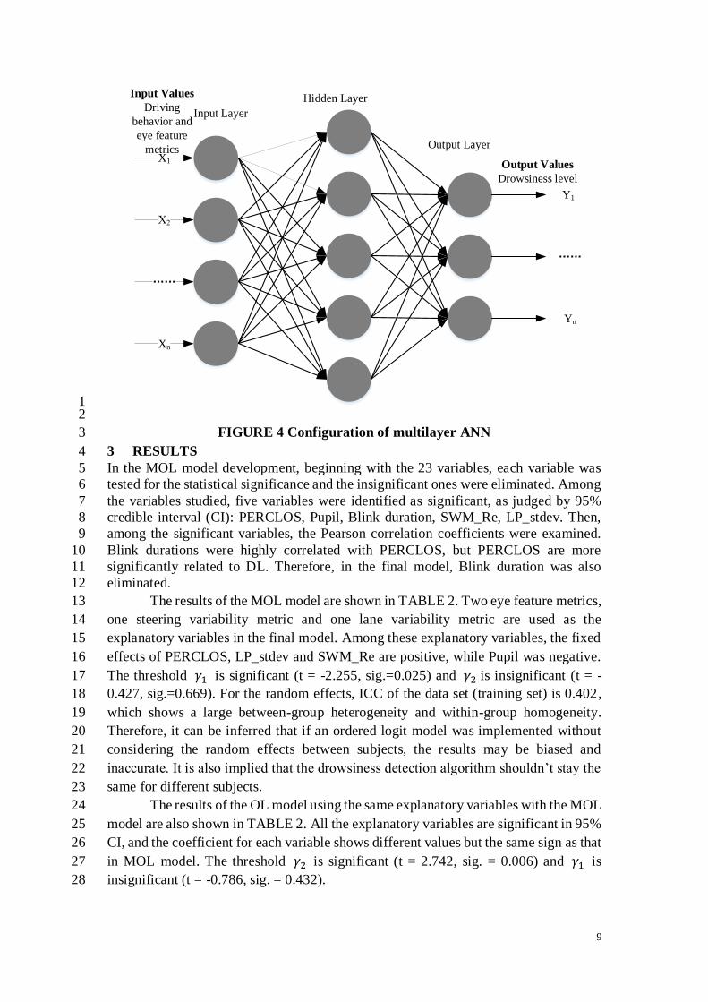
In this study, we built a feed-forward neural network with one hidden layer 29

8

consisting of the interconnection of neurons only between two adjacent layers. A back 1

propagation training method was used. Before modeling, the following standardization 2

procedure was carried out for each metric: 3

𝑥𝑖 =

𝑥𝑖 − 𝑥𝑚𝑖𝑛

𝑥𝑚𝑎𝑥 − 𝑥𝑚𝑖𝑛

(7)

A basic computational element is called a node. Each node receives input from 4

an external source or from other nodes. Each input has an associated weight (𝑤𝑖𝑗 ), 5

which can be modified to model synaptic learning by the process of training. The input 6

of the jth node in the hidden layer is calculated as follows: 7

𝑍𝑗 = ∑ 𝑤𝑖𝑗(𝑥𝑖 + 𝑏𝑗) 𝑖 = 1,2, … , 𝑁 𝑗 = 1,2, … , 𝑀

𝑖

(8)

Where 𝑍𝑗 is the input to jth node in the hidden layer, 𝑤𝑖𝑗 is the weight of ith node in 8

the input layer to jth node in the hidden layer, 𝑥𝑗 is the value of ith node in the input 9

layer, 𝑏𝑗 is bias value for the jth node in the hidden layer, N is the number of nodes in 10

the input layer, and M is the number of nodes in the hidden layer. 11

The output of a node is decided by its input as well as the activation function. 12

Different activation functions such as sigmoid functions, hyperbolic tangent functions, 13

and logistic functions can be used. A hyperbolic tangent function was used as the 14

activation function of the hidden layer in our study. It was calculated as follows: 15

𝐻𝑗 = 𝑓(𝑍𝑗) = tanh(𝑍𝑗) =

𝑒2𝑧𝑗 − 1

𝑒2𝑧𝑗 + 1 (9)

16

Where 𝐻𝑗 is the output of jth node in hidden layer. 17

In our study, we want the outputs of ANN to be interpretable as probabilities 18

for a categorical target variable (DL), for those outputs to lie between 0 and 1, and to 19

have a sum of 1. Therefore, a Softmax activation function is used for the output layer, 20

which is written as follows: 21

𝑂𝑘 =

exp(𝑍𝑘)

∑ exp(𝑍𝑚)𝑐𝑚=1

(10)

22

Where 𝑂𝑘 is the output of kth node in the output layer, c is the number of categories 23

for the target variable. 24

In the training process, the network output, in general, may not be equal to the 25

desired output. Therefore, the output error is calculated as the difference between the 26

network output and the desired output. If the output error does not satisfy the tolerance 27

level, the network modifies the connection weights (𝑤𝑖𝑗) according to the value of the 28

output error; then, training data is inputted again to the network and the network output 29

is calculated. The training cycle is continued until the network achieves the desired 30

tolerance level. 31

9

X1

……

Xn

Input Values

Driving

behavior and

eye feature

metrics

Input Layer

Hidden Layer

Output Layer

Y1

……

Yn

Output Values

Drowsiness level

1 2

FIGURE 4 Configuration of multilayer ANN 3

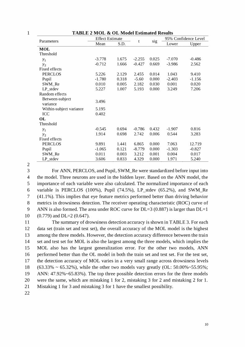
3 RESULTS 4

In the MOL model development, beginning with the 23 variables, each variable was 5

tested for the statistical significance and the insignificant ones were eliminated. Among 6

the variables studied, five variables were identified as significant, as judged by 95% 7

credible interval (CI): PERCLOS, Pupil, Blink duration, SWM_Re, LP_stdev. Then, 8

among the significant variables, the Pearson correlation coefficients were examined. 9

Blink durations were highly correlated with PERCLOS, but PERCLOS are more 10

significantly related to DL. Therefore, in the final model, Blink duration was also 11

eliminated. 12

The results of the MOL model are shown in TABLE 2. Two eye feature metrics, 13

one steering variability metric and one lane variability metric are used as the 14

explanatory variables in the final model. Among these explanatory variables, the fixed 15

effects of PERCLOS, LP_stdev and SWM_Re are positive, while Pupil was negative. 16

The threshold 𝛾1 is significant (t = -2.255, sig.=0.025) and 𝛾2 is insignificant (t = -17

0.427, sig.=0.669). For the random effects, ICC of the data set (training set) is 0.402, 18

which shows a large between-group heterogeneity and within-group homogeneity. 19

Therefore, it can be inferred that if an ordered logit model was implemented without 20

considering the random effects between subjects, the results may be biased and 21

inaccurate. It is also implied that the drowsiness detection algorithm shouldn’t stay the 22

same for different subjects. 23

The results of the OL model using the same explanatory variables with the MOL 24

model are also shown in TABLE 2. All the explanatory variables are significant in 95% 25

CI, and the coefficient for each variable shows different values but the same sign as that 26

in MOL model. The threshold 𝛾2 is significant (t = 2.742, sig. = 0.006) and 𝛾1 is 27

insignificant (t = -0.786, sig. = 0.432). 28

10

TABLE 2 MOL & OL Model Estimated Results 1

Parameters Effect Estimate

t sig 95% Confidence Level

Mean S.D. Lower Upper

MOL

Threshold

𝛾1 -3.778 1.675 -2.255 0.025 -7.070 -0.486

𝛾2 -0.712 1.666 -0.427 0.669 -3.986 2.562

Fixed effects

PERCLOS 5.226 2.129 2.455 0.014 1.043 9.410

Pupil -1.780 0.318 -5.60 0.000 -2.403 -1.156

SWM_Re 0.010 0.005 2.182 0.030 0.001 0.020

LP_stdev 5.227 1.007 5.193 0.000 3.249 7.206

Random effects

Between-subject

variance 3.496

Within-subject variance 5.195

ICC 0.402

OL

Threshold

𝛾1 -0.545 0.694 -0.786 0.432 -1.907 0.816

𝛾2 1.914 0.698 2.742 0.006 0.544 3.283

Fixed effects

PERCLOS 9.891 1.441 6.865 0.000 7.063 12.719

Pupil -1.065 0.121 -8.779 0.000 -1.303 -0.827

SWM_Re 0.011 0.003 3.212 0.001 0.004 0.017

LP_stdev 3.606 0.833 4.329 0.000 1.971 5.240

2

For ANN, PERCLOS, and Pupil, SWM_Re were standardized before input into 3

the model. Three neurons are used in the hidden layer. Based on the ANN model, the 4

importance of each variable were also calculated. The normalized importance of each 5

variable is PERCLOS (100%), Pupil (74.5%), LP_stdev (65.2%), and SWM_Re 6

(41.1%). This implies that eye feature metrics performed better than driving behavior 7

metrics in drowsiness detection. The receiver operating characteristic (ROC) curve of 8

ANN is also formed. The area under ROC curve for DL=3 (0.887) is larger than DL=1 9

(0.779) and DL=2 (0.647). 10

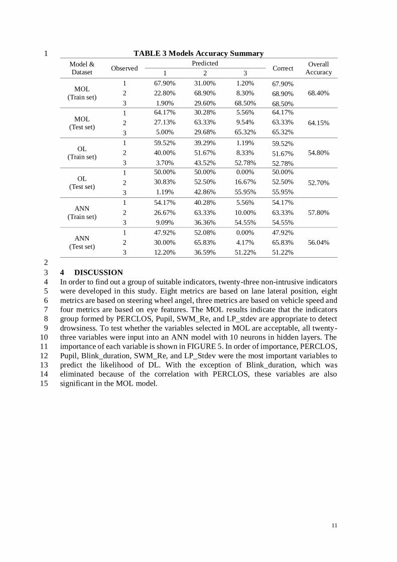
The summary of drowsiness detection accuracy is shown in TABLE 3. For each 11

data set (train set and test set), the overall accuracy of the MOL model is the highest 12

among the three models. However, the detection accuracy difference between the train 13

set and test set for MOL is also the largest among the three models, which implies the 14

MOL also has the largest generalization error. For the other two models, ANN 15

performed better than the OL model in both the train set and test set. For the test set, 16

the detection accuracy of MOL varies in a very small range across drowsiness levels 17

(63.33% ~ 65.32%), while the other two models vary greatly (OL: 50.00%~55.95%; 18

ANN: 47.92%~65.83%). The top three possible detection errors for the three models 19

were the same, which are mistaking 1 for 2, mistaking 3 for 2 and mistaking 2 for 1. 20

Mistaking 1 for 3 and mistaking 3 for 1 have the smallest possibility. 21

22

11

TABLE 3 Models Accuracy Summary 1

Model &

Dataset Observed

Predicted Correct

Overall

Accuracy 1 2 3

MOL

(Train set)

1 67.90% 31.00% 1.20% 67.90%

68.40% 2 22.80% 68.90% 8.30% 68.90%

3 1.90% 29.60% 68.50% 68.50%

MOL

(Test set)

1 64.17% 30.28% 5.56% 64.17%

64.15% 2 27.13% 63.33% 9.54% 63.33%

3 5.00% 29.68% 65.32% 65.32%

OL

(Train set)

1 59.52% 39.29% 1.19% 59.52%

54.80% 2 40.00% 51.67% 8.33% 51.67%

3 3.70% 43.52% 52.78% 52.78%

OL

(Test set)

1 50.00% 50.00% 0.00% 50.00%

52.70% 2 30.83% 52.50% 16.67% 52.50%

3 1.19% 42.86% 55.95% 55.95%

ANN

(Train set)

1 54.17% 40.28% 5.56% 54.17%

57.80% 2 26.67% 63.33% 10.00% 63.33%

3 9.09% 36.36% 54.55% 54.55%

ANN

(Test set)

1 47.92% 52.08% 0.00% 47.92%

56.04% 2 30.00% 65.83% 4.17% 65.83%

3 12.20% 36.59% 51.22% 51.22%

2

4 DISCUSSION 3

In order to find out a group of suitable indicators, twenty-three non-intrusive indicators 4

were developed in this study. Eight metrics are based on lane lateral position, eight 5

metrics are based on steering wheel angel, three metrics are based on vehicle speed and 6

four metrics are based on eye features. The MOL results indicate that the indicators 7

group formed by PERCLOS, Pupil, SWM_Re, and LP_stdev are appropriate to detect 8

drowsiness. To test whether the variables selected in MOL are acceptable, all twenty-9

three variables were input into an ANN model with 10 neurons in hidden layers. The 10

importance of each variable is shown in FIGURE 5. In order of importance, PERCLOS, 11

Pupil, Blink_duration, SWM_Re, and LP_Stdev were the most important variables to 12

predict the likelihood of DL. With the exception of Blink_duration, which was 13

eliminated because of the correlation with PERCLOS, these variables are also 14

significant in the MOL model. 15

12

1 FIGURE 5 Variables importance in ANN with all the metrics 2

3

According to FIGURE 5, the top three important variables are all eye feature 4

metrics. These results can be interpreted that eye feature metrics perform better than 5

driving behavior metrics in drowsiness detection. The following test also verified this 6

inference. After removing eye feature metrics, the detection accuracy of the ANN 7

model for the test set was reduced to 45.8%. Meanwhile, keeping only eye feature 8

metrics, the detection accuracy of the ANN model was reduced to 49.3%. Because of 9

this, some drowsiness detection studies have used only eye feature metrics to detect 10

drowsiness (10; 16). However, the detection accuracy of the ANN model using both 11

metrics has the highest detection accuracy. Use of driving behavior metrics is also 12

needed. Moreover, the eye features are often measured by cameral and image 13

processing, which may not be reliable. The driving behavior metrics can be a 14

supplement to increase the reliability of the detection system. 15

For driving behavior metrics, both lane related and steering related metrics are 16

important in the models. Among lane related metrics, the lane variability measure 17

(LP_stdev) performed better than other lane departure measures in drowsiness detection 18

models. The possible reason is the lane departure metrics only measure the features of 19

lane departure events and the lane variability information is missed for the non-20

departure parts. SWM_Re is the most important variable among steering related metrics, 21

which measures steering variability. Rapid steering wheel movement is suggested to be 22

a drowsiness measurement (18). In this study, it is measured by SWM_Rang_5 and is 23

not significant in the MOL model. Moreover, some studies (19) concluded the lane 24

variability is highly correlated with steering variability. We calculated the Pearson 25

correlation of SWM_Re and LP_stdev at 0.089 (sig. = 0.059), which indicates the 26

13

correlation between these variables is small. 1

In addition, previous research found there might be a curvilinear relationship 2

between KSS and drowsiness metrics (9), with a stronger change at high KSS levels 3

when compared with low KSS levels. In this study, among the four significant variables 4

in the MOL model, the mean change between DL 3 and DL 2 are larger than that 5

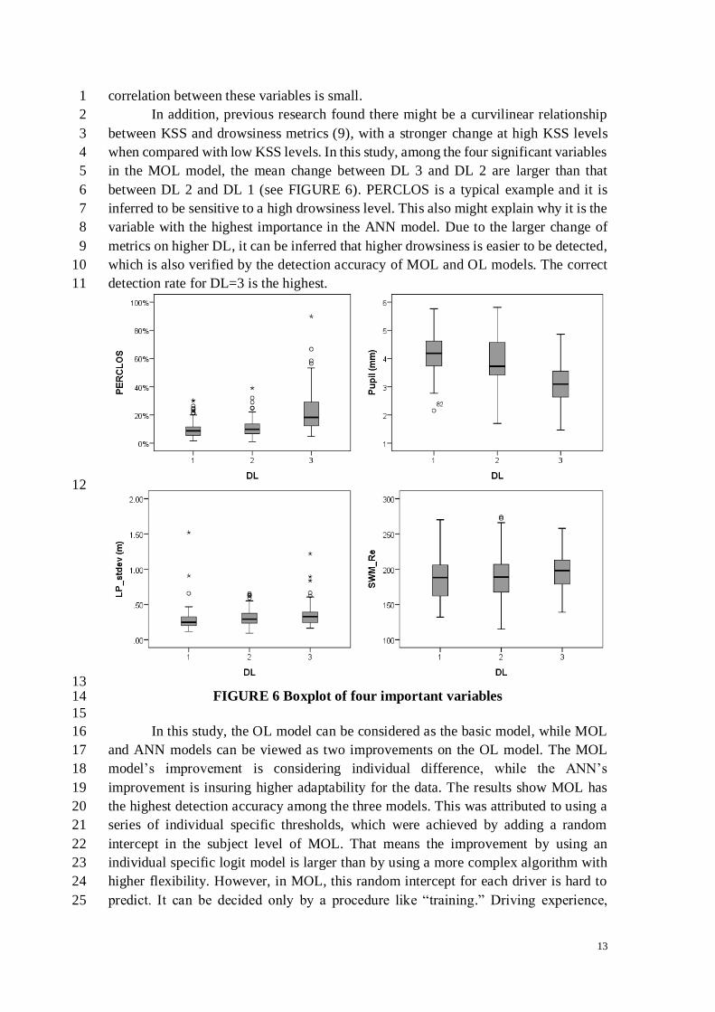
between DL 2 and DL 1 (see FIGURE 6). PERCLOS is a typical example and it is 6

inferred to be sensitive to a high drowsiness level. This also might explain why it is the 7

variable with the highest importance in the ANN model. Due to the larger change of 8

metrics on higher DL, it can be inferred that higher drowsiness is easier to be detected, 9

which is also verified by the detection accuracy of MOL and OL models. The correct 10

detection rate for DL=3 is the highest. 11

12

13 FIGURE 6 Boxplot of four important variables 14

15

In this study, the OL model can be considered as the basic model, while MOL 16

and ANN models can be viewed as two improvements on the OL model. The MOL 17

model’s improvement is considering individual difference, while the ANN’s 18

improvement is insuring higher adaptability for the data. The results show MOL has 19

the highest detection accuracy among the three models. This was attributed to using a 20

series of individual specific thresholds, which were achieved by adding a random 21

intercept in the subject level of MOL. That means the improvement by using an 22

individual specific logit model is larger than by using a more complex algorithm with 23

higher flexibility. However, in MOL, this random intercept for each driver is hard to 24

predict. It can be decided only by a procedure like “training.” Driving experience, 25

14

gender, age, and other characteristic variables of the driver were attempted as 1

explanations of individual differences, but no strong results were found. Yet the 2

individual difference is still the main obstacle to increasing the drowsiness detection 3

accuracy. 4

Some research that has classified drowsiness in only two levels (alert or drowsy) 5

has achieved high detection accuracy. But two levels of drowsiness aren’t enough to 6

support warning the driver before the crash risk becomes critical. Therefore, three levels 7

of drowsiness were used in this study. However, the detection accuracy is highly related 8

with lower numbers of drowsiness levels. If we used two levels of drowsiness (Level 1: 9

KSS 1~7; Level 2: 8~9), the detection accuracy increases from 64.15% to 88.6% for 10

the MOL model with the same variables, and the detection accuracy increases from 11

56.04 to 83.3% for ANN. It can be inferred that the more drowsiness levels to be 12

classified, the lower detection accuracy we would get in the models. Therefore, when 13

comparing the detection accuracy among detection models, the way to classify 14

drowsiness levels should also be considered. 15

16

5 CONCLUSION AND RECOMMENDATIONS 17

Twenty-three non-intrusive metrics including driving behavior and eye feature metrics 18

were evaluated in a simulated shift work study with a motion based high-fidelity driving 19

simulator in a controlled laboratory environment. Based on these metrics, MOL was 20

developed to detect three-level drowsiness. For comparison, two non-individual 21

specific models, OL and ANN, were also established. 22

MOL has the highest detection accuracy. This may be attributed to using a series 23

of individual specific criteria, which was achieved by adding a random intercept at the 24

subject level. Among the twenty-three variables, PERCLOS, Pupil, LP_stdev and 25

SWM_Re were significant in MOL and OL, and were also confirmed in ANN. Metrics 26

of eye features performed better (showed higher importance) in the drowsiness 27

detection models than other metrics, which was also verified using ANN by comparing 28

the detection accuracy between eye features only and driving behaviors only. We also 29

found higher DL is more easily detected because of higher heterogeneity between 30

adjacent DLs. 31

Based on the analysis, using a user-specific method to detect driver drowsiness 32

is recommended in order to address the inaccuracies caused by individual difference. 33

In this study, the group characteristics (like age, gender) of participants were controlled. 34

However, if group characteristics exist, we can build group-specific models that would 35

simplify the model training process by group determinants. Therefore group 36

characteristics are recommended for study. Also, because establishment of drowsiness 37

level in this research was subjective, more accurate measures should be applied, for 38

example, using EEG to determine drowsiness level. 39

40

ACKNOWLEDGEMENTS 41

Supported by Road and Traffic Engineering Key Laboratory of Tongji University, 42

Ministry of Education. 43

44

REFERENCES 45

1. NHTSA’s National Center for Statistics and Analysis. Traffic Safety Facts: A Brief 46

15

Statistical Summary. NHTSA, U.S. Department of Transportation. DOT HS 811 1

449, 2011. 2

2. Maycock, G. Sleepiness and Driving: the Experience of UK Car Drivers. Accident 3

Analysis & Prevention, Vol.29, No.4, 1997, No.453-462. 4

3. The Ministry of Public Security of the People’s Republic of China, Road and 5

Transport Authority. Road Traffic Crash Statistics 2001-2008, 2009. 6

4. Central Intelligence Agency, United States. The world factbook. 2010. Retrieved 7

2013. 8

5. Klauer, S. G., Dingus, T. A., Neale, V. L., Sudweeks, J. D., and Ramsey, D. J. The 9

Impact of Driver Inattention on Near-Crash/Crash Risk: An Analysis Using the 10

100-Car Naturalistic Driving Study Data. No. HS-810 594, 2006. 11

6. Radun, I., Ohisalo, J., Radun, J., Rajalin, S., 2012. Law Defining the Critical Level 12

of Driver Fatigue in Terms of Hours without Sleep: Criminal Justice Professionals' 13

Opinions and Fatal Accident Data. International Journal of Law, Crime and Justice, 14

Vol.40, No.3, 2012, pp.172-178. 15

7. Li, W., He, Q. C., Fan, X. M., and Fei, Z. M. Evaluation of Driver Fatigue on Two 16

Channels of EEG Data. Neuroscience Letters, Vol.506, No.2, 2012, pp.235-239. 17

8. Patel, M., Lal, S. K. L., Kavanagh, D., and Rossiter, P. Applying Neural Network 18

Analysis on Heart Rate Variability Data to Assess Driver Fatigue. Expert Systems 19

with Applications, Vol.38, No.6, 2011, pp.7235-7242. 20

9. Ingre, M., Åkerstedt, T., Peters, B., Anund, A., Kecklund, G. Subjective Sleepiness, 21

Simulated Driving Performance and Blink Duration: Examining Individual 22

Differences. Journal of Sleep Research, Vol.15, No.1, 2006, pp.47-53. 23

10. Jo, J., Lee, S. J., Park, K. R., Kim, I. J., and Kim, J. Detecting Driver Drowsiness 24

Using Feature-Level Fusion and User-Specific Classification. Expert Systems with 25

Applications, Vol.41, No.4, 2014, pp.1139-1152. 26

11. Ingre, M., ÅKerstedt, T., Peters, B., Anund, A., Kecklund, G., and Pickles, A. 27

Subjective Sleepiness and Accident Risk Avoiding the Ecological Fallacy. Journal 28

of sleep research, Vol.15, No.2, 2006, pp.142-148. 29

12. Thiffault P. and Bergeron J. Fatigue and Individual Differences in Monotonous 30

Simulated Driving. Personality and Individual Differences, Vol.34, No.1, 2003, 31

pp.159-176. 32

13. Hamada, T., Ito, T., Adachi, K., Nakano, T., and Yamamoto, S. Detecting Method 33

for Drivers' Drowsiness Applicable to Individual Features. In proceeding of 34

Intelligent Transportation Systems, Vol.2, 2003, pp.1405-1410. 35

14. Wierwille, W. W., Wreggit, S. S., Kirn, C. L., Ellsworth, L. A., and Fairbanks, R. 36

J. Research on Vehicle-Based Driver Status/Performance Monitoring; 37

Development, Validation, and Refinement of Algorithms for Detection of Driver 38

Drowsiness. DOT HS 808 247, 1994. 39

15. Yang, G., Lin, Y., and Bhattacharya, P. A Driver Fatigue Recognition Model Based 40

on Information Fusion and Dynamic Bayesian Network. Information Sciences, 41

Vol.180, No.10, 2010, pp.1942-1954. 42

16. Hu, S. and Zheng, G. Driver Drowsiness Detection with Eyelid Related Parameters 43

by Support Vector Machine. Expert Systems with Applications, Vol.36, No.4, 2009, 44

16

pp.7651-7658. 1

17. Åkerstedt, T., and Gillberg, M. Subjective and Objective Sleepiness in the Active 2

Individual. International Journal of Neuroscience, Vol.52, No.1-2, 1990, pp.29-37. 3

18. Sandberg, D. and Wahde, M. Particle Swarm Optimization of Feed Forward Neural 4

Networks for the Detection of Drowsy Driving. In Neural Networks. IEEE 5

International Joint Conference, 2008, pp.788-793. 6

19. Forsman, P. M., Vila, B. J., Short, R. A., Mott, C. G., and Van Dongen, H. Efficient 7

Driver Drowsiness Detection at Moderate Levels of Drowsiness. Accident Analysis 8

& Prevention, Vol.50, 2013, pp.341-350. 9