DRIVE TECHNOLOGY ENGINEERED FOR ROBOTICS

01

DRIVE TECHNOLOGY ENGINEERED FOR ROBOTICS

WE DRIVE YOUR COBOT

2

1. Company 32. Product Overview 5 2.1 Simplicity Box 6 2.2 Gearbox 7 2.3 Component Kit 8 2.4 Intelligent COBOT Module 93. Ordering Code 10 3.1 Strain Wave Gears 10 3.2 Ordering Code Intelligent COBOT Module 114. Technical Data 12 4.1 General Technical Data 12 4.2 Dimensions 13 4.3 Accuracy 20 4.4 Torsional Stiffness 20 4.5 Technical Data of the Output Bearing 215. Technical Data ICM 22 5.1 Structure of the ICM 22 5.2 Technical Data 23 5.3 Dimensions 256. Gear Selection Procedure 26 6.1 Basic Introduction 27 6.2 Pre-selection 27 6.3 Load Cycle-based Dimensioning 28 6.4 Stiffness-based Dimensioning 29 6.5 Efficiency Design Type C-MO, SB-MO, SB-HO and B-MC 30 6.6 Efficiency Design Type B-HO 30 6.7 Service Life Wave Generator Bearing 30 6.8 Service Life Output Bearing 31 6.9 Permissible Static Tilting Moment 32 6.10 Calculation of the Torsional Angle 33 6.11 No Load Starting Torque 34 6.12 No Load Running Torque 34 6.13 No Load Back Driving Torque 357. Notes and Explanations 368. Copyright and Disclaimer 39

CONTENTS

3

INNOWELLE GmbH is focused on the development, research, design, testing and the manufacturing process of precise strain wave gears as well as complete mechatronic systems such as our Intelligent COBOT Module ICM.

We are your competent premium partner in the development and production of gear technologies and drive technologies for the robotics industry and specialise in the production of small and medium production volumes at the highest quality level.

INNOWELLE IS THE SPECIALIST IN DRIVE TECHNOLOGY FOR ALL ROBOT MANUFACTURERS:

• Strain Wave Gear We focus on five sizes of precise strain wave gear types with a torque range between 18Nm and 372Nm. The gears are available as a component kit, gearbox type or simplicity gearbox type. The gears are also available with or without hollow shaft.

• Intelligent COBOT Module Our Intelligent COBOT Module ICM is available in five sizes. It is equipped with a precise strain wave gear, a tilting resistant cross roller bearing, an effective synchronous motor, a fail-safe brake, two position sensors and a controller with EtherCAT protocol or CANopen protocol.

1. COMPANY

STRENGTHS OF INNOWELLE GMBH AS YOUR PARTNER

• Extraordinary knowledge of strain wave gear technology• Engineering for Robotic Drive Technology

Mechanics, Mechatronic, Robot Joint Design, Strain wave gear integration, Motor, Brake, Sensors, Drivers ...• Flexibility in creation of customised solutions for robotics• Main focus on robotic application• Excellent market knowledge• Extensive network in robotics

4

INNOWELLE OFFERS ALL THE ESSENTIAL TECHNOLOGIES FOR MECHANICAL OR ELECTROMECHANICAL DRIVE SYSTEMS. OUR SERVICES COVER ALL AREAS OF MODERN DEVELOPMENT.

Research & development• New technologies for mechanical and

mechatronic drive technology• Optimisation of existing technologies

and expertise• Basic research and improvement

Engineering & design• Customer- and market-specific products • Modular systems and individually configurable

products • Fast pace of innovation • New product and business areas • Savings potential, reusable solutions

Prototype manufacturing• Manufacture and assembly of fully

functional drive systems • Models for planned series products• Optimisation for series production • Validation and verification of requirements

regarding technology and the final products • Rapid results concerning theoretically

developed solutions

Transfer of expertise to series production• Design and optimisation of the series production

and assembly process • Material flow and value flow analyses • Machine and process capabilities• Support in quality assurance and development of

Kaizen Continuous Improvement Process, and the achievement of quality management objectives

Planning, project management and pre-development• Scheduling and resource planning • Process orientation and structuring• Periodic controlling and support until

the successful completion of the project

Service life and durability tests• Testing materials, components and systems • Inspections to prevent component failure • Static and dynamic strength hypotheses • Failure criteria, damage assessments and

lifetime estimates• Increasing the operational and design strength

of the components

5

We offer you a wide range of products with strain wave technology designed in Germany. Through collaboration with our partners for components, manufacturing parts and assembly in the European Union, in the USA and in Asia we are able to provide fully integrated products and total drive solutions.

The product range of INNOWELLE GmbH is the ideal choice for solving any motion task.

The main features of all our products are:• Excellent positioning accuracy• Zero backlash• High torque capacity• Lifelong precision• High single stage gear ratio• Compact and lightweight

2. PRODUCT OVERVIEW

WE DRIVE YOUR COBOT

6

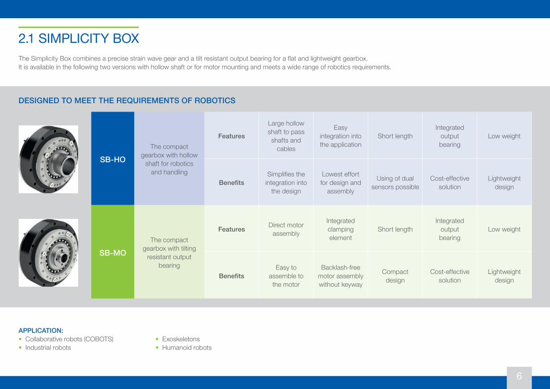
• Collaborative robots (COBOTS)• Industrial robots

• Exoskeletons• Humanoid robots

The Simplicity Box combines a precise strain wave gear and a tilt resistant output bearing for a flat and lightweight gearbox. It is available in the following two versions with hollow shaft or for motor mounting and meets a wide range of robotics requirements.

APPLICATION:

2.1 SIMPLICITY BOX

SB-HOThe compact

gearbox with hollow shaft for robotics

and handling

Features

Large hollow shaft to pass shafts and

cables

Easy integration into the application

Short lengthIntegrated

output bearing

Low weight

BenefitsSimplifies the

integration into the design

Lowest effort for design and

assembly

Using of dual sensors possible

Cost-effectivesolution

Lightweight design

SB-MOThe compact

gearbox with tilting resistant output

bearing

Features Direct motor assembly

Integrated clamping element

Short lengthIntegrated

output bearing

Low weight

BenefitsEasy to

assemble to the motor

Backlash-free motor assembly without keyway

Compact design

Cost-effective solution

Lightweight design

DESIGNED TO MEET THE REQUIREMENTS OF ROBOTICS

7

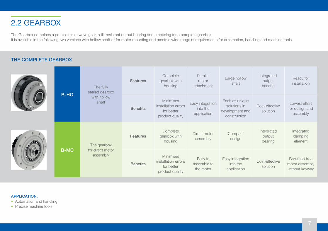
• Automation and handling• Precise machine tools

The Gearbox combines a precise strain wave gear, a tilt resistant output bearing and a housing for a complete gearbox. It is available in the following two versions with hollow shaft or for motor mounting and meets a wide range of requirements for automation, handling and machine tools.

APPLICATION:

2.2 GEARBOX

B-HOThe fully

sealed gearbox with hollow

shaft

FeaturesComplete

gearbox with housing

Parallel motor

attachment

Large hollow shaft

Integrated output bearing

Ready for installation

Benefits

Minimises installation errors

for better product quality

Easy integration into the

application

Enables unique solutions in

development and construction

Cost-effectivesolution

Lowest effort for design and

assembly

B-MCThe gearbox

for direct motor assembly

FeaturesComplete

gearbox with housing

Direct motor assembly

Compact design

Integrated output bearing


Benefits

Minimises installation errors

for better product quality

Easy to assemble to the motor

Easy integration into the

application

Cost-effective solution


THE COMPLETE GEARBOX

8

• Robotics• Automation and handling• Precise machine tools

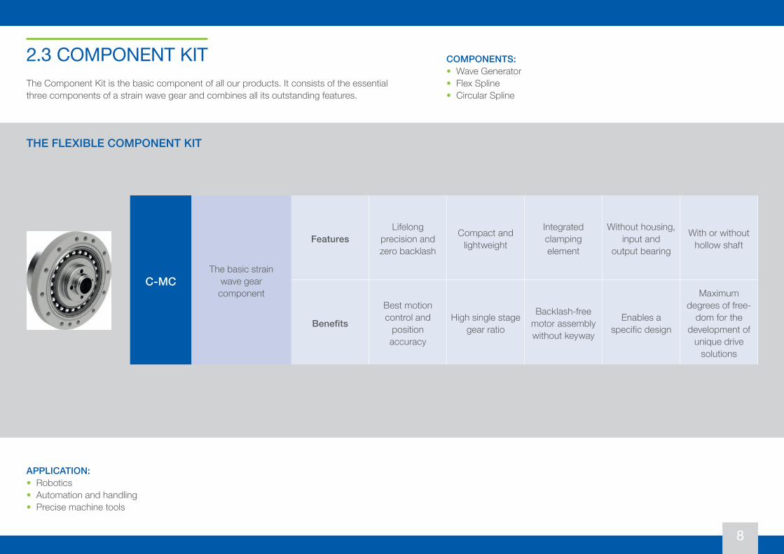
The Component Kit is the basic component of all our products. It consists of the essential three components of a strain wave gear and combines all its outstanding features.

APPLICATION:

2.3 COMPONENT KIT

C-MCThe basic strain

wave gear component

FeaturesLifelong

precision and zero backlash

Compact and lightweight


Without housing, input and

output bearing

With or without hollow shaft

Benefits

Best motion control and

position accuracy

High single stage gear ratio


Enables a specific design

Maximum degrees of free-

dom for the development of

unique drive solutions

THE FLEXIBLE COMPONENT KIT

• Wave Generator• Flex Spline• Circular Spline

COMPONENTS:

9

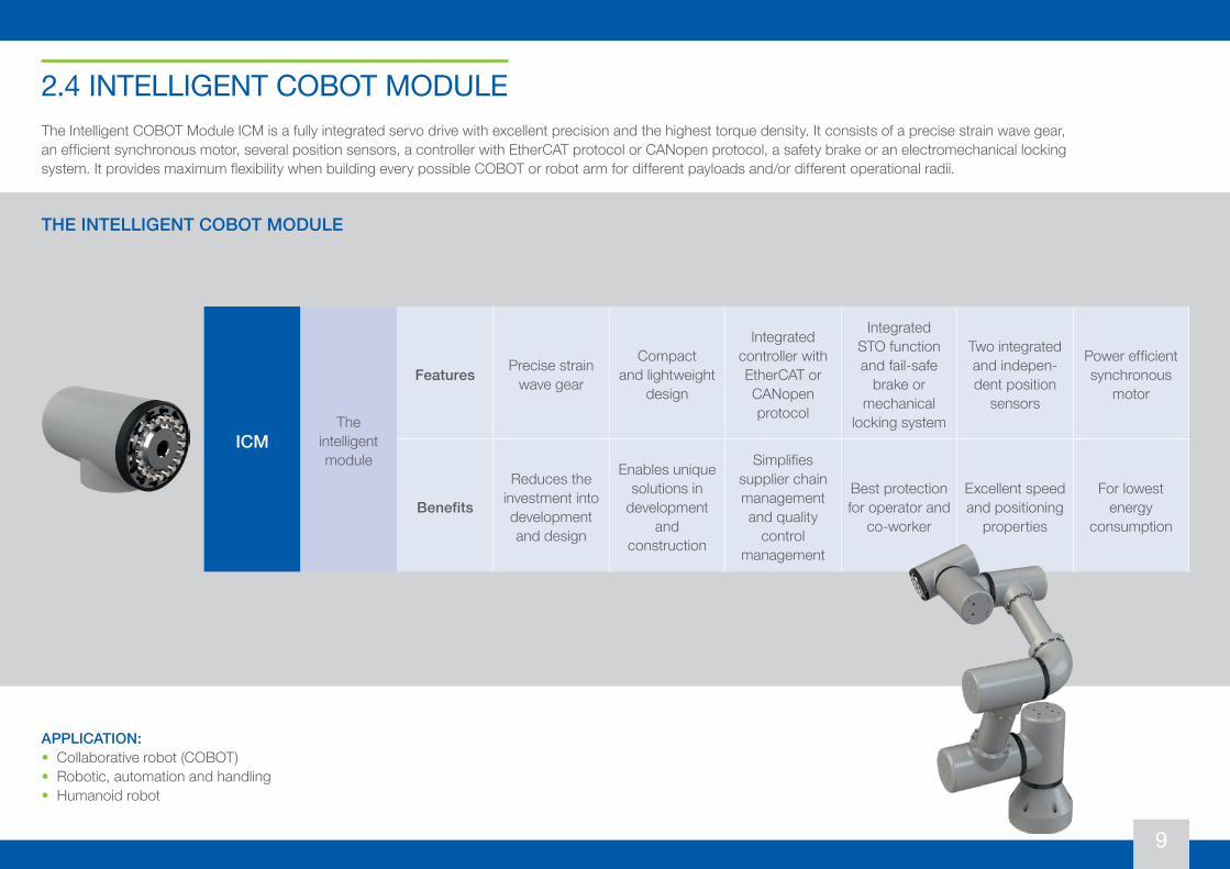
• Collaborative robot (COBOT)• Robotic, automation and handling• Humanoid robot

The Intelligent COBOT Module ICM is a fully integrated servo drive with excellent precision and the highest torque density. It consists of a precise strain wave gear, an efficient synchronous motor, several position sensors, a controller with EtherCAT protocol or CANopen protocol, a safety brake or an electromechanical locking system. It provides maximum flexibility when building every possible COBOT or robot arm for different payloads and/or different operational radii.

APPLICATION:

2.4 INTELLIGENT COBOT MODULE

ICMThe

intelligent module

Features Precise strain wave gear

Compact and lightweight

design

Integrated controller with EtherCAT or CANopen protocol

Integrated STO function and fail-safe

brake or mechanical

locking system

Two integrated and indepen-dent position

sensors

Power efficient synchronous

motor

Benefits

Reduces the investment into development and design

Enables unique solutions in

development and

construction

Simplifies supplier chain management and quality

control management

Best protection for operator and

co-worker

Excellent speed and positioning

properties

For lowest energy

consumption

THE INTELLIGENT COBOT MODULE

10

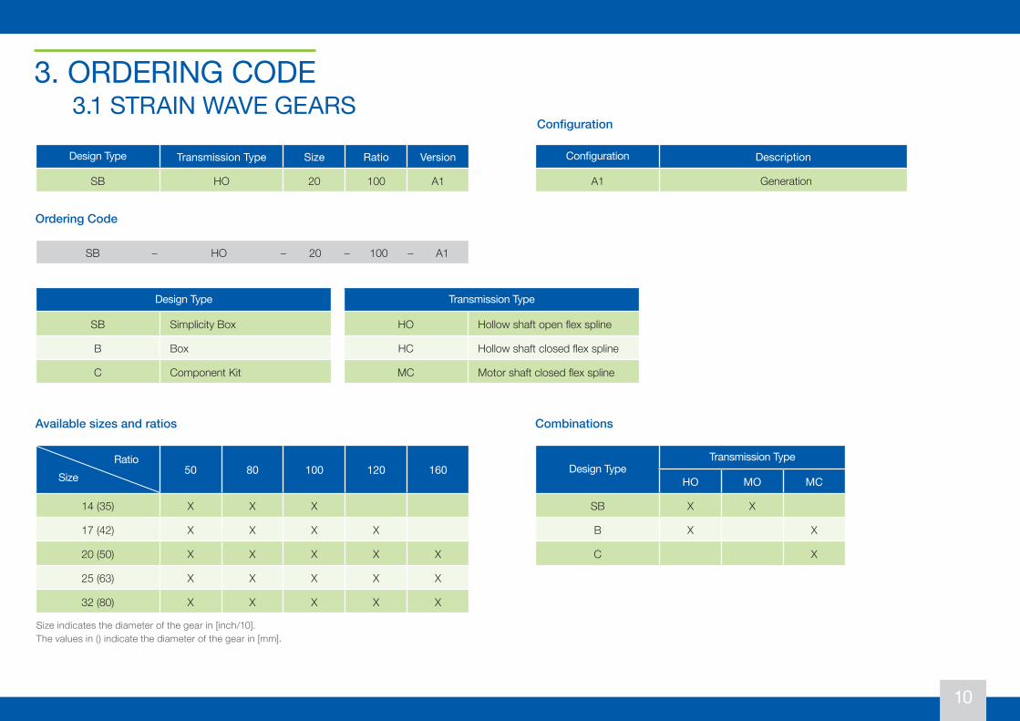
3. ORDERING CODE3.1 STRAIN WAVE GEARS

Design Type Transmission Type Size Ratio Version

SB HO 20 100 A1

SB – HO – 20 – 100 – A1

Ordering Code

Design Type

SB Simplicity Box

B Box

C Component Kit

Transmission Type

HO Hollow shaft open flex spline

HC Hollow shaft closed flex spline

MC Motor shaft closed flex spline

Available sizes and ratios

50 80 100 120 160

14 (35) X X X

17 (42) X X X X

20 (50) X X X X X

25 (63) X X X X X

32 (80) X X X X X

Combinations

Size indicates the diameter of the gear in [inch/10]. The values in () indicate the diameter of the gear in [mm].

Design TypeTransmission Type

HO MO MC

SB X X

B X X

C X

RatioSize

Configuration Description

A1 Generation

Configuration

11

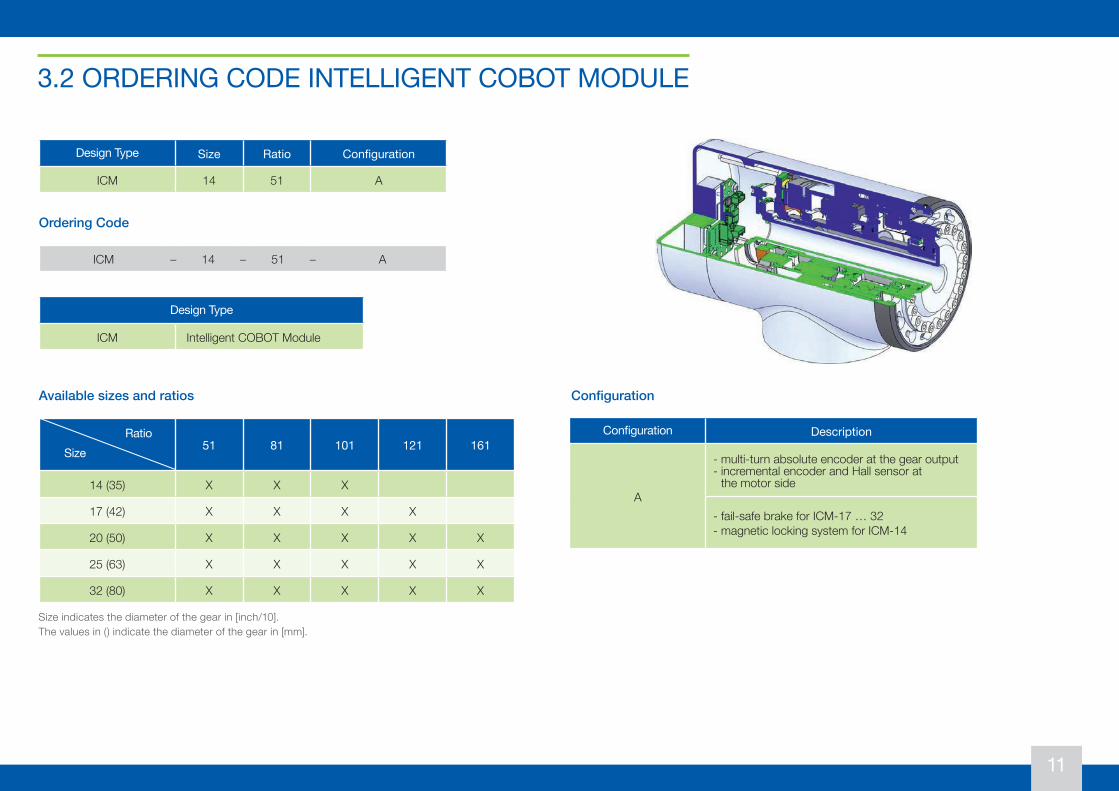
3.2 ORDERING CODE INTELLIGENT COBOT MODULE

Design Type Size Ratio Configuration

ICM 14 51 A

Configuration Description

A

- multi-turn absolute encoder at the gear output- incremental encoder and Hall sensor at

the motor side

- fail-safe brake for ICM-17 … 32- magnetic locking system for ICM-14

ICM – 14 – 51 – A

Ordering Code

Configuration

Design Type

ICM Intelligent COBOT Module

Available sizes and ratios

51 81 101 121 161

14 (35) X X X

17 (42) X X X X

20 (50) X X X X X

25 (63) X X X X X

32 (80) X X X X X


RatioSize

12

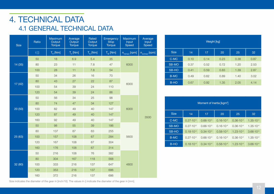
4. TECHNICAL DATA 4.1 GENERAL TECHNICAL DATA

SizeRatio

Maximum Output Torque

Average Output Torque

RatedOutput Torque

Emergency Stop

Torque

Maximum Input

Speed

Average Input

Speed

i [ ] TR [Nm] TA [Nm] TN [Nm] TM [Nm] nin(max) [rpm] nav(max) [rpm]

14 (35)

50 18 6.9 5.4 35

6000

3500

80 23 11 7.8 47

100 28 11 7.8 54

17 (42)

50 34 26 16 70

600080 43 27 22 87

100 54 39 24 110

120 54 39 24 86

20 (50)

50 56 34 25 98

6000

80 74 47 34 127

100 82 49 40 147

120 87 49 40 147

160 92 49 40 147

25 (63)

50 98 55 39 186

5600

80 137 87 63 255

100 157 108 67 284

120 167 108 67 304

160 176 108 67 314

32 (80)

50 216 108 76 382

4800

80 304 167 118 568

100 333 216 137 647

120 353 216 137 686

160 372 216 137 686


Weight [kg]

Size 14 17 20 25 32

C-MC 0.10 0.14 0.23 0.38 0.87

SB-MO 0.37 0.52 0.72 1.20 2.53

SB-HO 0.41 0.59 0.83 1.39 2.87

B-MC 0.49 0.62 0.89 1.40 3.02

B-HO 0.67 0.92 1.35 2.05 4.14

Moment of Inertia [kgm2]

Size 14 17 20 25 32

C-MC 0.27·10-5 0.66·10-5 0.16·10-4 0.36·10-4 1.35·10-4

SB-MO 0.27·10-5 0.66·10-5 0.16·10-4 0.36·10-4 1.35·10-4

SB-HO 0.18·10-4 0.34·10-4 0.58·10-4 1.23·10-4 3.66·10-4

B-MC 0.27·10-5 0.66·10-5 0.16·10-4 0.36·10-4 1.35·10-4

B-HO 0.18·10-4 0.34·10-4 0.58·10-4 1.23·10-4 3.66·10-4

13

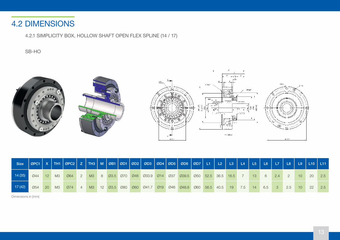
4.2 DIMENSIONS4.2.1 SIMPLICITY BOX, HOLLOW SHAFT OPEN FLEX SPLINE (14 / 17)

Size ØPC1 X TH1 ØPC2 Z TH3 M ØB1 ØD1 ØD2 ØD3 ØD4 ØD5 ØD6 ØD7 L1 L2 L3 L4 L5 L6 L7 L8 L9 L10 L11

14 (35) Ø44 12 M3 Ø64 2 M3 8 Ø3.5 Ø70 Ø48 Ø33.9 Ø14 Ø37 Ø39.5 Ø50 52.5 36.5 16.5 7 13 6 2.4 2 10 20 2.5

17 (42) Ø54 20 M3 Ø74 4 M3 12 Ø3.5 Ø80 Ø60 Ø41.7 Ø19 Ø46 Ø48.8 Ø60 56.5 40.5 19 7.5 14 6.5 3 2.5 10 22 2.5

Dimensions in [mm]

SB-HO

14

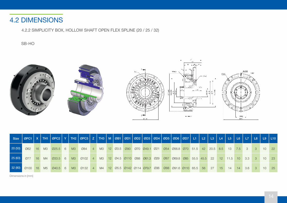
4.2 DIMENSIONS4.2.2 SIMPLICITY BOX, HOLLOW SHAFT OPEN FLEX SPLINE (20 / 25 / 32)

Size ØPC1 X TH1 ØPC2 Y TH2 ØPC3 Z TH3 M ØB1 ØD1 ØD2 ØD3 ØD4 ØD5 ØD6 ØD7 L1 L2 L3 L4 L5 L6 L7 L8 L9 L10

20 (50) Ø62 16 M3 Ø25.5 6 M3 Ø84 4 M3 12 Ø3.5 Ø90 Ø70 Ø49.1 Ø21 Ø54 Ø56.8 Ø70 51.5 42 20.5 8.5 13 7.5 3 3 10 22

25 (63) Ø77 16 M4 Ø33.5 6 M3 Ø102 4 M3 12 Ø4.5 Ø110 Ø88 Ø61.3 Ø29 Ø67 Ø69.8 Ø85 55.5 45.5 22 12 11.5 10 3.3 3 10 23

32 (80) Ø100 16 M5 Ø40.5 6 M3 Ø132 4 M4 12 Ø5.5 Ø142 Ø114 Ø79.7 Ø36 Ø88 Ø91.6 Ø110 65.5 56 27 15 14 14 3.6 3 10 25

Dimensions in [mm]

SB-HO

15

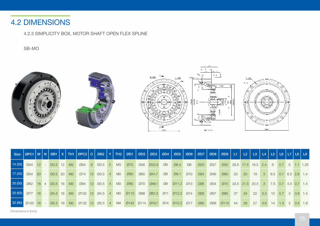
4.2.3 SIMPLICITY BOX, MOTOR SHAFT OPEN FLEX SPLINE

Size ØPC1 M N ØB1 X TH1 ØPC2 O ØB2 Y TH2 ØD1 ØD2 ØD3 ØD4 ØD5 ØD6 ØD7 ØD8 ØD9 L1 L2 L3 L4 L5 L6 L7 L8 L9

14 (35) Ø44 12 - Ø3.5 12 M3 Ø64 8 Ø3.5 2 M3 Ø70 Ø48 Ø33.9 Ø6 Ø6.4 Ø8 Ø20 Ø37 Ø50 28.5 17.5 16.5 2.4 6 0.7 5 1.1 1.25

17 (42) Ø54 20 - Ø3.5 20 M3 Ø74 12 Ø3.5 4 M3 Ø80 Ø60 Ø41.7 Ø8 Ø9.1 Ø10 Ø24 Ø46 Ø60 33 20 19 3 6.5 0.7 6.5 2.6 1.4

20 (50) Ø62 16 4 Ø3.5 16 M3 Ø84 12 Ø3.5 4 M3 Ø90 Ø70 Ø49.1 Ø9 Ø11.2 Ø13 Ø26 Ø54 Ø70 33.5 21.5 20.5 3 7.5 0.7 4.5 0.7 1.4

25 (63) Ø77 16 - Ø4.5 16 M4 Ø102 12 Ø4.5 4 M3 Ø110 Ø88 Ø61.3 Ø11 Ø12.2 Ø14 Ø28 Ø67 Ø85 37 24 22 3.3 10 0.7 3 0.8 1.4

32 (80) Ø100 16 - Ø5.5 16 M5 Ø132 12 Ø5.5 4 M4 Ø142 Ø114 Ø79.7 Ø14 Ø15.2 Ø17 Ø35 Ø88 Ø110 44 28 27 3.6 14 1.3 2 0.5 1.8

Dimensions in [mm]

4.2 DIMENSIONS

SB-MO

16

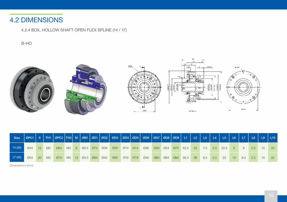
4.2.4 BOX, HOLLOW SHAFT OPEN FLEX SPLINE (14 / 17)

Size ØPC1 X TH1 ØPC2 TH2 M ØB1 ØD1 ØD2 ØD3 ØD4 ØD5 ØD6 ØD7 ØD8 ØD9 L1 L2 L3 L4 L5 L6 L7 L8 L9 L10

14 (35) Ø44 12 M3 Ø64 M3 8 Ø3.5 Ø74 Ø36 Ø20 Ø14 Ø14 Ø36 Ø50 Ø54 Ø70 52.5 33 7.5 5.5 20.5 9 8 2.5 10 20

17 (42) Ø54 20 M3 Ø74 M3 12 Ø3.5 Ø84 Ø45 Ø25 Ø19 Ø19 Ø45 Ø60 Ø64 Ø80 56.5 36 8.5 5.5 23 10 8.5 2.5 10 22

Dimensions in [mm]

4.2 DIMENSIONS

B-HO

17

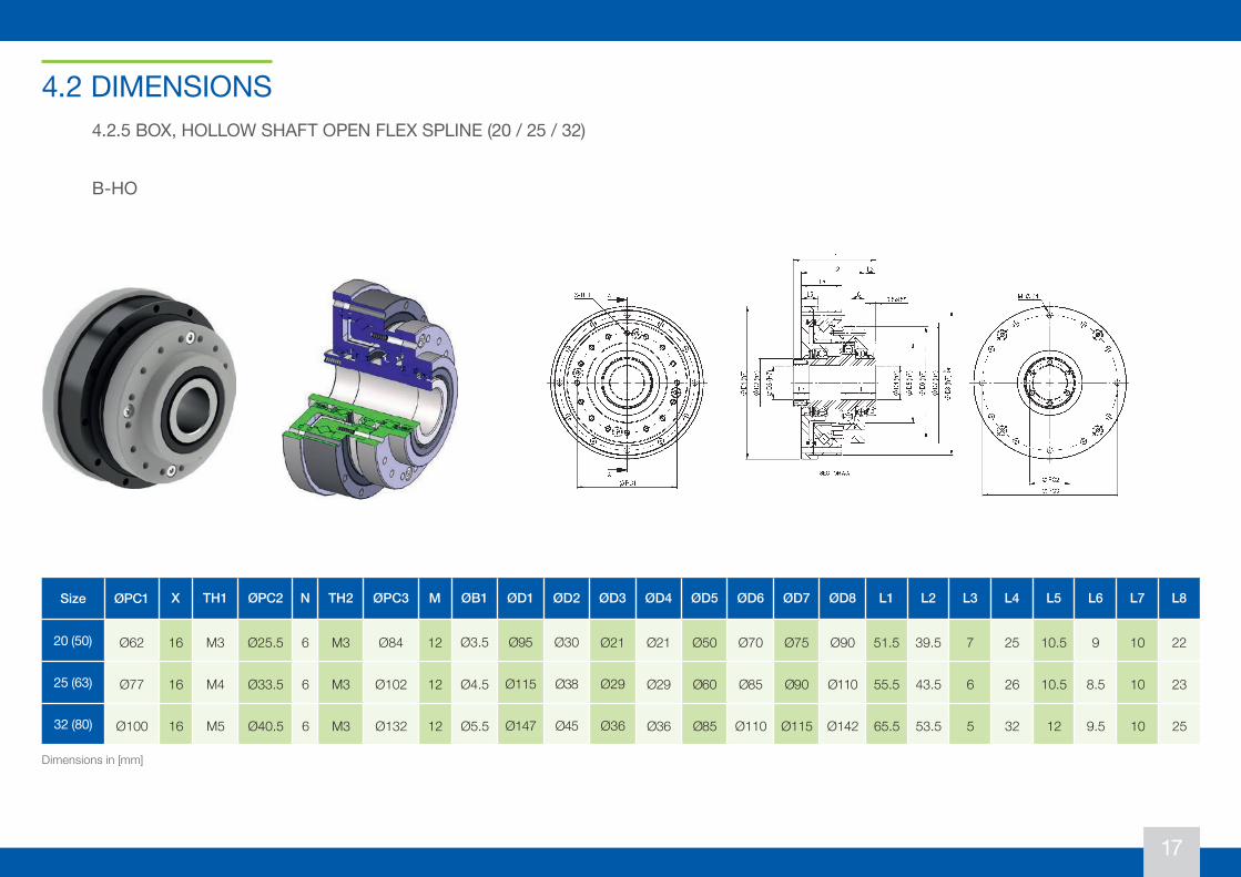
4.2.5 BOX, HOLLOW SHAFT OPEN FLEX SPLINE (20 / 25 / 32)

Size ØPC1 X TH1 ØPC2 N TH2 ØPC3 M ØB1 ØD1 ØD2 ØD3 ØD4 ØD5 ØD6 ØD7 ØD8 L1 L2 L3 L4 L5 L6 L7 L8

20 (50) Ø62 16 M3 Ø25.5 6 M3 Ø84 12 Ø3.5 Ø95 Ø30 Ø21 Ø21 Ø50 Ø70 Ø75 Ø90 51.5 39.5 7 25 10.5 9 10 22

25 (63) Ø77 16 M4 Ø33.5 6 M3 Ø102 12 Ø4.5 Ø115 Ø38 Ø29 Ø29 Ø60 Ø85 Ø90 Ø110 55.5 43.5 6 26 10.5 8.5 10 23

32 (80) Ø100 16 M5 Ø40.5 6 M3 Ø132 12 Ø5.5 Ø147 Ø45 Ø36 Ø36 Ø85 Ø110 Ø115 Ø142 65.5 53.5 5 32 12 9.5 10 25

Dimensions in [mm]

4.2 DIMENSIONS

B-HO

18

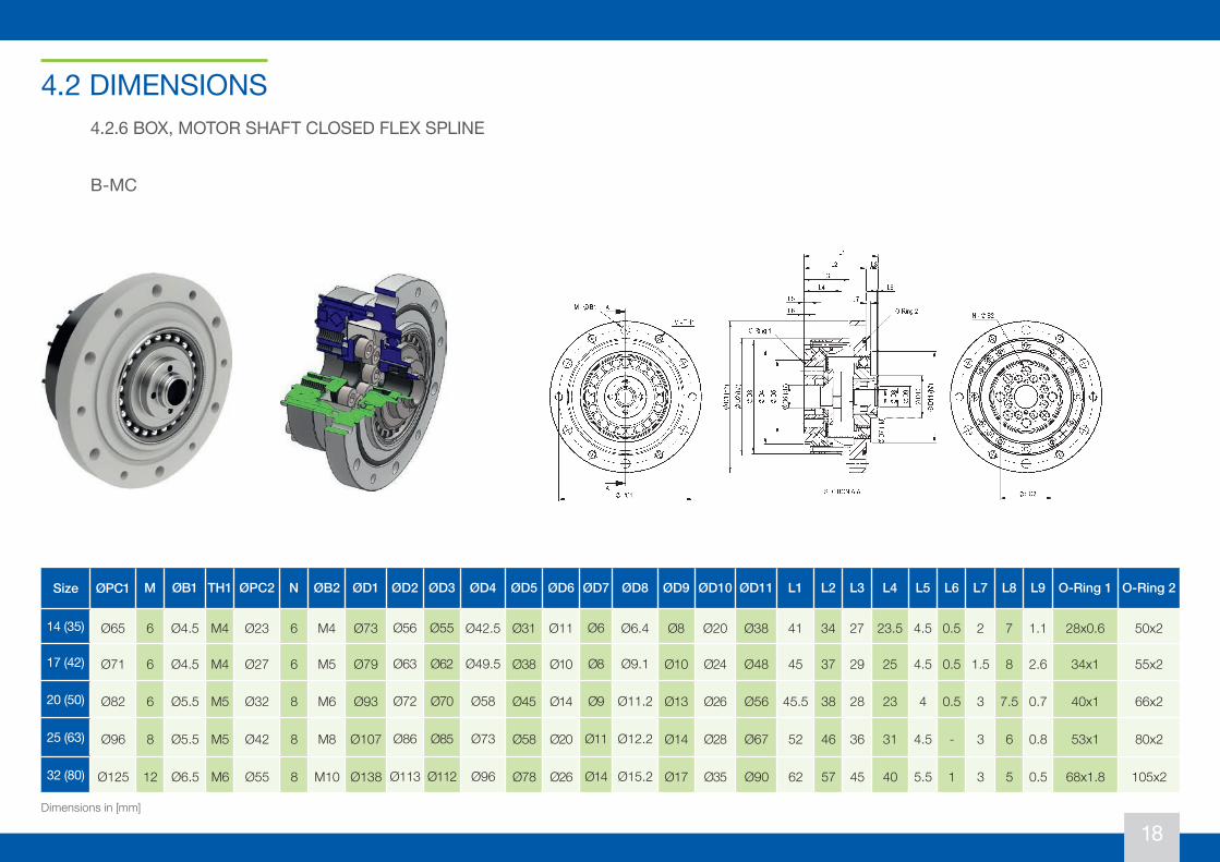
4.2.6 BOX, MOTOR SHAFT CLOSED FLEX SPLINE

Size ØPC1 M ØB1 TH1 ØPC2 N ØB2 ØD1 ØD2 ØD3 ØD4 ØD5 ØD6 ØD7 ØD8 ØD9 ØD10 ØD11 L1 L2 L3 L4 L5 L6 L7 L8 L9 O-Ring 1 O-Ring 2

14 (35) Ø65 6 Ø4.5 M4 Ø23 6 M4 Ø73 Ø56 Ø55 Ø42.5 Ø31 Ø11 Ø6 Ø6.4 Ø8 Ø20 Ø38 41 34 27 23.5 4.5 0.5 2 7 1.1 28x0.6 50x2

17 (42) Ø71 6 Ø4.5 M4 Ø27 6 M5 Ø79 Ø63 Ø62 Ø49.5 Ø38 Ø10 Ø8 Ø9.1 Ø10 Ø24 Ø48 45 37 29 25 4.5 0.5 1.5 8 2.6 34x1 55x2

20 (50) Ø82 6 Ø5.5 M5 Ø32 8 M6 Ø93 Ø72 Ø70 Ø58 Ø45 Ø14 Ø9 Ø11.2 Ø13 Ø26 Ø56 45.5 38 28 23 4 0.5 3 7.5 0.7 40x1 66x2

25 (63) Ø96 8 Ø5.5 M5 Ø42 8 M8 Ø107 Ø86 Ø85 Ø73 Ø58 Ø20 Ø11 Ø12.2 Ø14 Ø28 Ø67 52 46 36 31 4.5 - 3 6 0.8 53x1 80x2

32 (80) Ø125 12 Ø6.5 M6 Ø55 8 M10 Ø138 Ø113 Ø112 Ø96 Ø78 Ø26 Ø14 Ø15.2 Ø17 Ø35 Ø90 62 57 45 40 5.5 1 3 5 0.5 68x1.8 105x2

Dimensions in [mm]

4.2 DIMENSIONS

B-MC

19

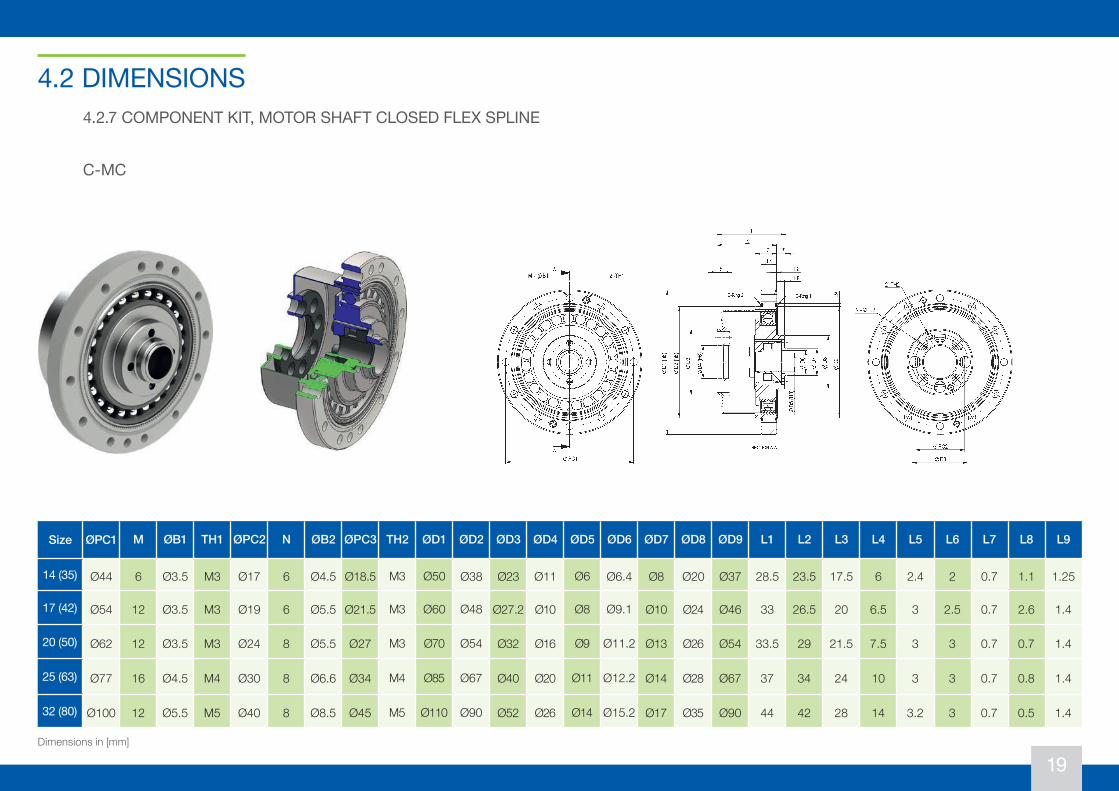
4.2.7 COMPONENT KIT, MOTOR SHAFT CLOSED FLEX SPLINE

Size ØPC1 M ØB1 TH1 ØPC2 N ØB2 ØPC3 TH2 ØD1 ØD2 ØD3 ØD4 ØD5 ØD6 ØD7 ØD8 ØD9 L1 L2 L3 L4 L5 L6 L7 L8 L9

14 (35) Ø44 6 Ø3.5 M3 Ø17 6 Ø4.5 Ø18.5 M3 Ø50 Ø38 Ø23 Ø11 Ø6 Ø6.4 Ø8 Ø20 Ø37 28.5 23.5 17.5 6 2.4 2 0.7 1.1 1.25

17 (42) Ø54 12 Ø3.5 M3 Ø19 6 Ø5.5 Ø21.5 M3 Ø60 Ø48 Ø27.2 Ø10 Ø8 Ø9.1 Ø10 Ø24 Ø46 33 26.5 20 6.5 3 2.5 0.7 2.6 1.4

20 (50) Ø62 12 Ø3.5 M3 Ø24 8 Ø5.5 Ø27 M3 Ø70 Ø54 Ø32 Ø16 Ø9 Ø11.2 Ø13 Ø26 Ø54 33.5 29 21.5 7.5 3 3 0.7 0.7 1.4

25 (63) Ø77 16 Ø4.5 M4 Ø30 8 Ø6.6 Ø34 M4 Ø85 Ø67 Ø40 Ø20 Ø11 Ø12.2 Ø14 Ø28 Ø67 37 34 24 10 3 3 0.7 0.8 1.4

32 (80) Ø100 12 Ø5.5 M5 Ø40 8 Ø8.5 Ø45 M5 Ø110 Ø90 Ø52 Ø26 Ø14 Ø15.2 Ø17 Ø35 Ø90 44 42 28 14 3.2 3 0.7 0.5 1.4

Dimensions in [mm]

4.2 DIMENSIONS

C-MC

20

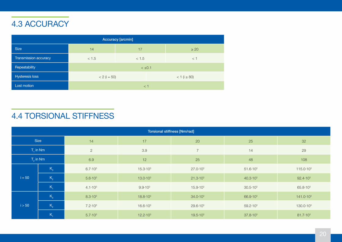
4.3 ACCURACY

4.4 TORSIONAL STIFFNESS

Accuracy [arcmin]

Size 14 17 ≥ 20

Transmission accuracy < 1.5 < 1.5 < 1

Repeatability < ±0.1

Hysteresis loss < 2 (i = 50) < 1 (i ≥ 80)

Lost motion < 1

Torsional stiffness [Nm/rad]

Size 14 17 20 25 32

T1 in Nm 2 3.9 7 14 29

T2 in Nm 6.9 12 25 48 108

i = 50

K3 6.7·103 15.3·103 27.0·103 51.6·103 115.0·103

K2 5.6·103 13.0·103 21.3·103 40.3·103 92.4·103

K1 4.1·103 9.9·103 15.9·103 30.5·103 65.8·103

i > 50

K3 8.3·103 18.8·103 34.0·103 66.9·103 141.0·103

K2 7.2·103 16.6·103 29.6·103 59.2·103 130.0·103

K1 5.7·103 12.2·103 19.5·103 37.8·103 81.7·103

21

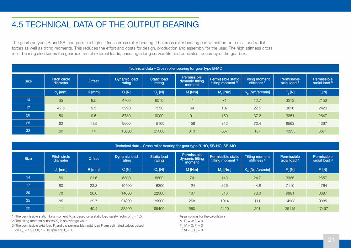
The gearbox types B and SB incorporate a high stiffness cross roller bearing. The cross roller bearing can withstand both axial and radial forces as well as tilting moments. This reduces the effort and costs for design, production and assembly for the user. The high stiffness cross roller bearing also keeps the gearbox free of external loads, ensuring a long service life and consistent accuracy of the gearbox.

4.5 TECHNICAL DATA OF THE OUTPUT BEARING

Technical data – Cross roller bearing for gear type B-HO, SB-HO, SB-MO

Size Pitch circle diameter Offset Dynamic load

ratingStatic load

ratingPermissible

dynamic tilting moment

Permissible static tilting moment 1)

Tilting moment stiffness 2)

Permissible axial load 3)

Permissible radial load 3)

dp [mm] R [mm] C [N] C0 [N] M [Nm] M0 [Nm] KB [Nm/arcmin] Fa [N] Fr [N]

14 50 21.6 5800 8600 74 143 24.7 3965 2657

17 60 22.3 10400 16300 124 326 44.8 7110 4764

20 70 26.6 14600 22000 187 513 73.3 9981 6687

25 85 29.7 21800 35800 258 1014 111 14903 9985

32 111 40.4 38200 65400 580 2420 291 26115 17497

Technical data – Cross roller bearing for gear type B-MC

Size Pitch circle diameter Offset Dynamic load

ratingStatic load

ratingPermissible

dynamic tilting moment

Permissible static tilting moment 1)

Tilting moment stiffness 2)

Permissible axial load 3)

Permissible radial load 3)

dp [mm] R [mm] C [N] C0 [N] M [Nm] M0 [Nm] KB [Nm/arcmin] Fa [N] Fr [N]

14 35 9.5 4700 6070 41 71 12.7 3213 2153

17 42.5 9.5 5290 7550 64 107 22.5 3616 2423

20 50 9.5 5780 9000 91 150 37.2 3951 2647

25 62 11.5 9600 15100 156 312 70.4 6563 4397

32 80 14 15000 25000 313 667 157 10255 6871

1) The permissible static tilting moment M0 is based on a static load safety factor of fs = 1.5.2) The tilting moment stiffness KB is an average value. 3) The permissible axial load Fa and the permissible radial load Fr are estimated values based

on L10 = 15000h, n = 15 rpm and fw = 1.

Assumptions for the calculation:M: Fa = 0; Fr = 0Fa: M = 0; Fr = 0Fr: M = 0; Fa = 0

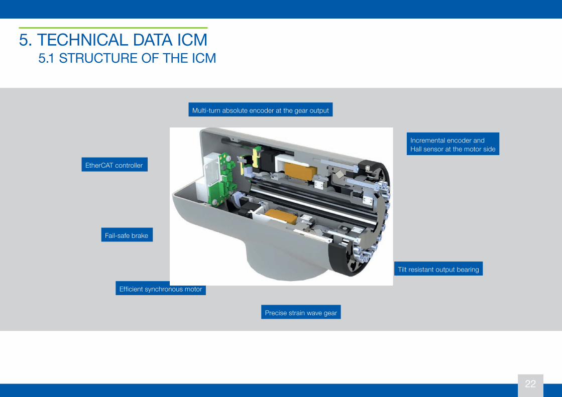
22

Multi-turn absolute encoder at the gear output

Incremental encoder and Hall sensor at the motor side

EtherCAT controller

Precise strain wave gear

Efficient synchronous motor

Fail-safe brake

Tilt resistant output bearing

5. TECHNICAL DATA ICM5.1 STRUCTURE OF THE ICM

23

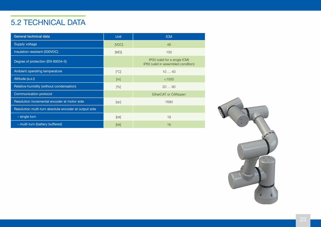
5.2 TECHNICAL DATAGeneral technical data Unit ICM

Supply voltage [VDC] 48

Insulation resistant (500VDC) [MΩ] 100

Degree of protection (EN 60034-5) IP00 (valid for a single ICM)IP65 (valid in assembled condition)

Ambient operating temperature [°C] 10 … 40

Altitude (a.s.l) [m] <1000

Relative humidity (without condensation) [%] 20 … 80

Communication protocol EtherCAT or CANopen

Resolution incremental encoder at motor side [qc] 7680

Resolution multi-turn absolute encoder at output side

– single turn [bit] 19

– multi-turn (battery buffered) [bit] 16

24

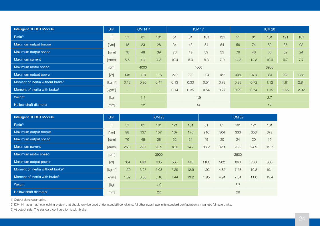
1) Output via circular spline 2) ICM-14 has a magnetic locking system that should only be used under standstill conditions. All other sizes have in its standard configuration a magnetic fail-safe brake.3) At output side. The standard configuration is with brake.

Intelligent COBOT Module Unit ICM 14 2) ICM 17 ICM 20

Ratio1) [ ] 51 81 101 51 81 101 121 51 81 101 121 161

Maximum output torque [Nm] 18 23 28 34 43 54 54 56 74 82 87 92

Maximum output speed [rpm] 78 49 39 78 49 39 33 76 48 38 32 24

Maximum current [Arms] 5.5 4.4 4.3 10.4 8.3 8.3 7.0 14.8 12.3 10.9 9.7 7.7

Maximum motor speed [rpm] 4000 4000 3900

Maximum output power [W] 148 119 116 279 222 224 187 448 373 331 293 233

Moment of inertia without brake3) [kgm²] 0.12 0.30 0.47 0.13 0.33 0.51 0.73 0.29 0.72 1.12 1.61 2.84

Moment of inertia with brake3) [kgm²] - - - 0.14 0.35 0.54 0.77 0.29 0.74 1.15 1.65 2.92

Weight [kg] 1.3 1.9 2.7

Hollow shaft diameter [mm] 12 14 17

Intelligent COBOT Module Unit ICM 25 ICM 32

Ratio1) [ ] 51 81 101 121 161 51 81 101 121 161

Maximum output torque [Nm] 98 137 157 167 176 216 304 333 353 372

Maximum output speed [rpm] 76 48 38 32 24 49 30 24 20 15

Maximum current [Arms] 25.8 22.7 20.9 18.6 14.7 36.2 32.1 28.2 24.9 19.7

Maximum motor speed [rpm] 3900 2500

Maximum output power [W] 784 690 635 563 446 1108 982 863 763 605

Moment of inertia without brake3) [kgm²] 1.30 3.27 5.08 7.29 12.9 1.92 4.85 7.53 10.8 19.1

Moment of inertia with brake3) [kgm²] 1.32 3.33 5.18 7.44 13.2 1.95 4.91 7.64 11.0 19.4

Weight [kg] 4.0 6.7

Hollow shaft diameter [mm] 22 26

25

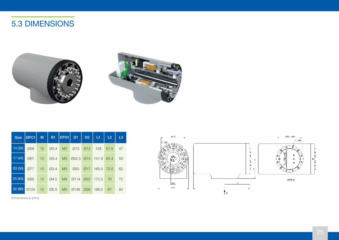
5.3 DIMENSIONS

Size ØPC1 M B1 ØTH1 D1 D2 L1 L2 L3

14 (35) Ø58 12 Ø3.4 M3 Ø73 Ø12 128 57.5 47

17 (42) Ø67 12 Ø3.4 M3 Ø82.5 Ø14 141.9 62.4 50

20 (50) Ø77 12 Ø3.4 M3 Ø93 Ø17 160.5 72.5 62

25 (63) Ø95 12 Ø4.5 M4 Ø114 Ø22 172.5 70 72

32 (80) Ø124 12 Ø5.5 M5 Ø146 Ø26 186.5 87 84

Dimensions in [mm]

26

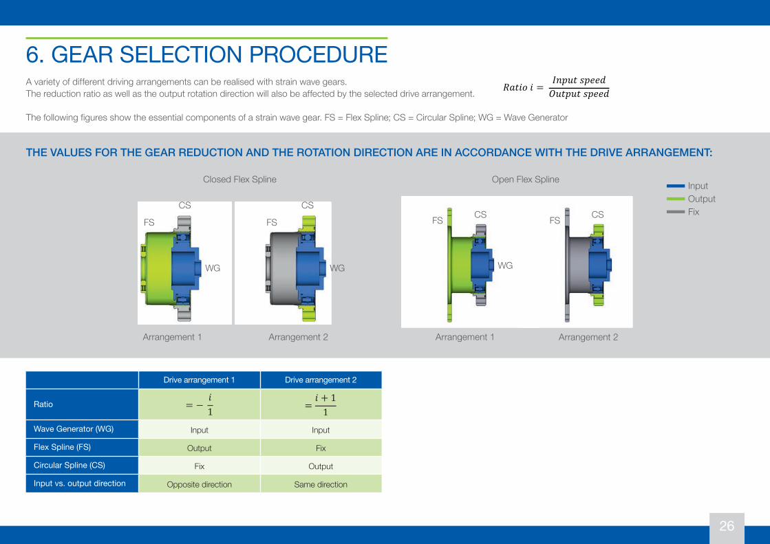
6. GEAR SELECTION PROCEDUREA variety of different driving arrangements can be realised with strain wave gears. The reduction ratio as well as the output rotation direction will also be affected by the selected drive arrangement. 𝑅𝑅𝑅𝑅𝑅𝑅𝑅𝑅𝑅𝑅𝑅𝑅 =

𝐼𝐼𝐼𝐼𝐼𝐼𝐼𝐼𝑅𝑅𝑠𝑠𝐼𝐼𝑠𝑠𝑠𝑠𝑠𝑠𝑂𝑂𝐼𝐼𝑅𝑅𝐼𝐼𝐼𝐼𝑅𝑅𝑠𝑠𝐼𝐼𝑠𝑠𝑠𝑠𝑠𝑠

The following figures show the essential components of a strain wave gear. FS = Flex Spline; CS = Circular Spline; WG = Wave Generator

WG

Closed Flex Spline

Arrangement 1Arrangement 1

CS CSCS CS

FS FS FS FS

Arrangement 2Arrangement 2

Open Flex Spline

WG WGWG

InputOutput Fix

Drive arrangement 1 Drive arrangement 2

Ratio

Wave Generator (WG) Input Input

Flex Spline (FS) Output Fix

Circular Spline (CS) Fix Output

Input vs. output direction Opposite direction Same direction

THE VALUES FOR THE GEAR REDUCTION AND THE ROTATION DIRECTION ARE IN ACCORDANCE WITH THE DRIVE ARRANGEMENT:

26

6. Gear Selection ProcedureA variety of different driving arrangements can be realized with strain wave gears. The reduction ratio as well as the output rotation direction will also be affected by the selected drive arrangement.

𝑅𝑅𝑅𝑅𝑅𝑅𝑅𝑅𝑅𝑅𝑅𝑅 = 𝐼𝐼𝐼𝐼𝐼𝐼𝐼𝐼𝑅𝑅𝑠𝑠𝐼𝐼𝑠𝑠𝑠𝑠𝑠𝑠𝑂𝑂𝐼𝐼𝑅𝑅𝐼𝐼𝐼𝐼𝑅𝑅𝑠𝑠𝐼𝐼𝑠𝑠𝑠𝑠𝑠𝑠

The following figures shows the essential components of a strain wave gear. FS = Flex Spline; CS = Circular Spline; WG = Wave Generator

The values for the gear reduction and the rotation direction are in accordance to the drive arrangement:

Version: Closed Flex Spline Open Flex Spline

Input Output

Fix


Ratio = −𝑖𝑖1 =

𝑖𝑖 + 11





FS CS CS

FS

WG WG WG WG

CS CS FS FS

Arrangement 1 Arrangement 2


26

6. Gear Selection ProcedureA variety of different driving arrangements can be realized with strain wave gears. The reduction ratio as well as the output rotation direction will also be affected by the selected drive arrangement.

𝑅𝑅𝑅𝑅𝑅𝑅𝑅𝑅𝑅𝑅𝑅𝑅 = 𝐼𝐼𝐼𝐼𝐼𝐼𝐼𝐼𝑅𝑅𝑠𝑠𝐼𝐼𝑠𝑠𝑠𝑠𝑠𝑠𝑂𝑂𝐼𝐼𝑅𝑅𝐼𝐼𝐼𝐼𝑅𝑅𝑠𝑠𝐼𝐼𝑠𝑠𝑠𝑠𝑠𝑠

The following figures shows the essential components of a strain wave gear. FS = Flex Spline; CS = Circular Spline; WG = Wave Generator

The values for the gear reduction and the rotation direction are in accordance to the drive arrangement:

Version: Closed Flex Spline Open Flex Spline

Input Output

Fix


Ratio = −𝑖𝑖1 =

𝑖𝑖 + 11





FS CS CS

FS

WG WG WG WG

CS CS FS FS



27

Depending on the application, the required torque or stiffness can be the decisive criterion when selecting the gearbox. Nevertheless, it is essential that both torque and stiffness are taken into account when designing the gearbox. Please follow the procedure outlined below to get the exact gearbox you need for your application.

You should consider these questions when pre-selecting the gear:

Are the core elements of the gearbox enough for me or do I want to use the output bearing recommended by INNOWELLE? Ideally, directly with seals and housing covers, so that I can install the gear directly without any problems. • C-Component kit (Core elements) • SB-Simplicity box (Component kit + output bearing) • B-Box (Simplicity box + shaft bearing + seals + housing cover)

Do I need a hollow shaft or a motor shaft at the drive side?• H-Version (Hollow shaft)• M-Version (Motor shaft)

What is the needed acceleration torque, deceleration torque and the needed continuous torque that occur in my application? The necessary torques of the application determine the gear size.• 14 / 17 / 20 / 25 / 32

What are the maximum speed and average speed that occur in my application? The necessary speed of the application determines the gearbox reduction ratio. • 50 / 80 / 100 / 120 /160

6.1 BASIC INTRODUCTION

6.2 PRE-SELECTION

28

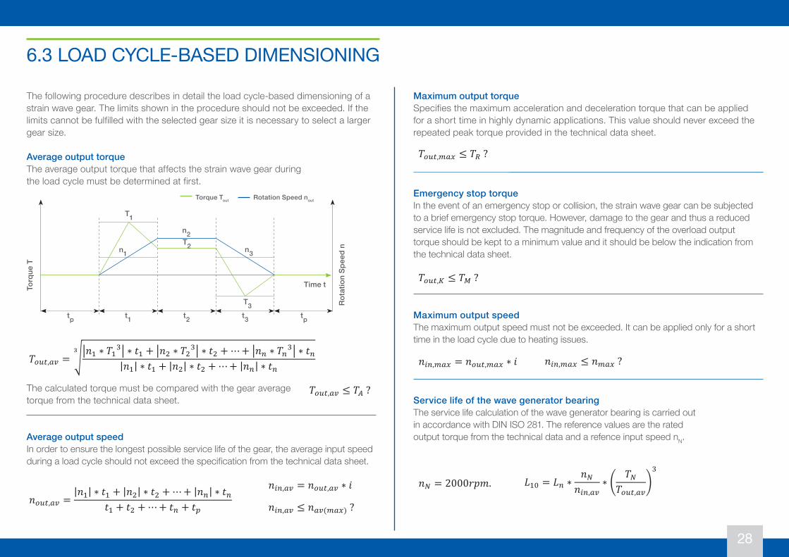
The following procedure describes in detail the load cycle-based dimensioning of a strain wave gear. The limits shown in the procedure should not be exceeded. If the limits cannot be fulfilled with the selected gear size it is necessary to select a larger gear size.

Average output torqueThe average output torque that affects the strain wave gear during the load cycle must be determined at first.

Maximum output torqueSpecifies the maximum acceleration and deceleration torque that can be applied for a short time in highly dynamic applications. This value should never exceed the repeated peak torque provided in the technical data sheet.

Emergency stop torque In the event of an emergency stop or collision, the strain wave gear can be subjected to a brief emergency stop torque. However, damage to the gear and thus a reduced service life is not excluded. The magnitude and frequency of the overload output torque should be kept to a minimum value and it should be below the indication from the technical data sheet.

Maximum output speed The maximum output speed must not be exceeded. It can be applied only for a short time in the load cycle due to heating issues.

Service life of the wave generator bearing The service life calculation of the wave generator bearing is carried out in accordance with DIN ISO 281. The reference values are the rated output torque from the technical data and a refence input speed nN.

6.3 LOAD CYCLE-BASED DIMENSIONING

The calculated torque must be compared with the gear average torque from the technical data sheet.

Average output speedIn order to ensure the longest possible service life of the gear, the average input speed during a load cycle should not exceed the specification from the technical data sheet.

T3tp t1

T1

n1

n2

n3

Time t

Rot

atio

n Sp

eed

n

Torq

ue T

t2 t3 tp

T2

Torque Tout Rotation Speed nout

28

6.3 Load Cycle Based Dimensioning

The following procedure describes in detail the load cycle-based dimensioning of a strain wave gear. The limits shown in the procedure should not be exceeded. If the limits can not be fulfilled with the selected gear size it is necessary to select a larger gear size. Average Output Torque The average output torque that affects the strain wave gear during the load cycle must be determined at first.

𝑇𝑇!"#,%& = 12𝑛𝑛' ∗ 𝑇𝑇'(2 ∗ 𝑡𝑡' + 2𝑛𝑛) ∗ 𝑇𝑇)(2 ∗ 𝑡𝑡) + ⋯+ 2𝑛𝑛* ∗ 𝑇𝑇*(2 ∗ 𝑡𝑡*|𝑛𝑛'| ∗ 𝑡𝑡' + |𝑛𝑛)| ∗ 𝑡𝑡) + ⋯+ |𝑛𝑛*| ∗ 𝑡𝑡*

!


𝑇𝑇!"#,%& ≤ 𝑇𝑇+?

Average output speed In order to ensure the longest possible service life of the gear, the average input speedduring a load cycle should not exceed the specification from the technical data sheet.

𝑛𝑛!"#,%& =|𝑛𝑛'| ∗ 𝑡𝑡' + |𝑛𝑛)| ∗ 𝑡𝑡) + ⋯+ |𝑛𝑛*| ∗ 𝑡𝑡*

𝑡𝑡' + 𝑡𝑡) + ⋯+ 𝑡𝑡* + 𝑡𝑡,

𝑛𝑛-*,%& = 𝑛𝑛!"#,%& ∗ 𝑖𝑖

𝑛𝑛-*,%& ≤ 𝑛𝑛%&(/%0)?

Maximum output torque Specifies the maximum acceleration and deceleration torque that can be applied for a short time in highly dynamic applications. This value should never exceed the repeated peak torque provided in the technical data sheet.

𝑇𝑇!"#,/%0 ≤ 𝑇𝑇2 ?

Torq

ue T

Time t

n1

n2

n3

Rot

atio

n S

peed

n

T1

T2

T3

Torque Tout

Rotation Speed nout

t1 t2 t3 tptp

29


𝑇𝑇!"#,3 ≤ 𝑇𝑇4?


𝑛𝑛-*,/%0 = 𝑛𝑛!"#,/%0 ∗ 𝑖𝑖

𝑛𝑛-*,/%0 ≤ 𝑛𝑛/%0?

Service life of the wave generator bearing The service life calculation of the wave generator bearing is carried out in accordance with DIN ISO 281. The reference values are the rated output torque from the technical data and a refence input speed of 𝑛𝑛5 = 2000𝑟𝑟𝑟𝑟𝑟𝑟.

𝐿𝐿'6 = 𝐿𝐿* ∗𝑛𝑛5

𝑛𝑛-*,%&∗ ?

𝑇𝑇5𝑇𝑇!"#,%&

@(

29


𝑇𝑇!"#,3 ≤ 𝑇𝑇4?


𝑛𝑛-*,/%0 = 𝑛𝑛!"#,/%0 ∗ 𝑖𝑖

𝑛𝑛-*,/%0 ≤ 𝑛𝑛/%0?



𝑛𝑛-*,%&∗ ?

𝑇𝑇5𝑇𝑇!"#,%&

@(

29


𝑇𝑇!"#,3 ≤ 𝑇𝑇4?


𝑛𝑛-*,/%0 = 𝑛𝑛!"#,/%0 ∗ 𝑖𝑖

𝑛𝑛-*,/%0 ≤ 𝑛𝑛/%0?



𝑛𝑛-*,%&∗ ?

𝑇𝑇5𝑇𝑇!"#,%&

@(

29


𝑇𝑇!"#,3 ≤ 𝑇𝑇4?


𝑛𝑛-*,/%0 = 𝑛𝑛!"#,/%0 ∗ 𝑖𝑖

𝑛𝑛-*,/%0 ≤ 𝑛𝑛/%0?



𝑛𝑛-*,%&∗ ?

𝑇𝑇5𝑇𝑇!"#,%&

@(

29


𝑇𝑇!"#,3 ≤ 𝑇𝑇4?


𝑛𝑛-*,/%0 = 𝑛𝑛!"#,/%0 ∗ 𝑖𝑖

𝑛𝑛-*,/%0 ≤ 𝑛𝑛/%0?



𝑛𝑛-*,%&∗ ?

𝑇𝑇5𝑇𝑇!"#,%&

@(

28




!


𝑇𝑇!"#,%& ≤ 𝑇𝑇+?


𝑛𝑛!"#,%& =|𝑛𝑛'| ∗ 𝑡𝑡' + |𝑛𝑛)| ∗ 𝑡𝑡) + ⋯+ |𝑛𝑛*| ∗ 𝑡𝑡*

𝑡𝑡' + 𝑡𝑡) + ⋯+ 𝑡𝑡* + 𝑡𝑡,

𝑛𝑛-*,%& = 𝑛𝑛!"#,%& ∗ 𝑖𝑖

𝑛𝑛-*,%& ≤ 𝑛𝑛%&(/%0)?


𝑇𝑇!"#,/%0 ≤ 𝑇𝑇2 ?

Torq

ue T

Time t

n1

n2

n3

Rot

atio

n S

peed

n

T1

T2

T3

Torque Tout

Rotation Speed nout

t1 t2 t3 tptp

28




!


𝑇𝑇!"#,%& ≤ 𝑇𝑇+?


𝑛𝑛!"#,%& =|𝑛𝑛'| ∗ 𝑡𝑡' + |𝑛𝑛)| ∗ 𝑡𝑡) + ⋯+ |𝑛𝑛*| ∗ 𝑡𝑡*

𝑡𝑡' + 𝑡𝑡) + ⋯+ 𝑡𝑡* + 𝑡𝑡,

𝑛𝑛-*,%& = 𝑛𝑛!"#,%& ∗ 𝑖𝑖

𝑛𝑛-*,%& ≤ 𝑛𝑛%&(/%0)?


𝑇𝑇!"#,/%0 ≤ 𝑇𝑇2 ?

Torq

ue T

Time t

n1

n2

n3

Rot

atio

n S

peed

n

T1

T2

T3

Torque Tout

Rotation Speed nout

t1 t2 t3 tptp

28




!


𝑇𝑇!"#,%& ≤ 𝑇𝑇+?


𝑛𝑛!"#,%& =|𝑛𝑛'| ∗ 𝑡𝑡' + |𝑛𝑛)| ∗ 𝑡𝑡) + ⋯+ |𝑛𝑛*| ∗ 𝑡𝑡*

𝑡𝑡' + 𝑡𝑡) + ⋯+ 𝑡𝑡* + 𝑡𝑡,

𝑛𝑛-*,%& = 𝑛𝑛!"#,%& ∗ 𝑖𝑖

𝑛𝑛-*,%& ≤ 𝑛𝑛%&(/%0)?


𝑇𝑇!"#,/%0 ≤ 𝑇𝑇2 ?

Torq

ue T

Time t

n1

n2

n3

Rot

atio

n S

peed

n

T1

T2

T3

Torque Tout

Rotation Speed nout

t1 t2 t3 tptp

28




!


𝑇𝑇!"#,%& ≤ 𝑇𝑇+?


𝑛𝑛!"#,%& =|𝑛𝑛'| ∗ 𝑡𝑡' + |𝑛𝑛)| ∗ 𝑡𝑡) + ⋯+ |𝑛𝑛*| ∗ 𝑡𝑡*

𝑡𝑡' + 𝑡𝑡) + ⋯+ 𝑡𝑡* + 𝑡𝑡,

𝑛𝑛-*,%& = 𝑛𝑛!"#,%& ∗ 𝑖𝑖

𝑛𝑛-*,%& ≤ 𝑛𝑛%&(/%0)?


𝑇𝑇!"#,/%0 ≤ 𝑇𝑇2 ?

Torq

ue T

Time t

n1

n2

n3

Rot

atio

n S

peed

n

T1

T2

T3

Torque Tout

Rotation Speed nout

t1 t2 t3 tptp

29

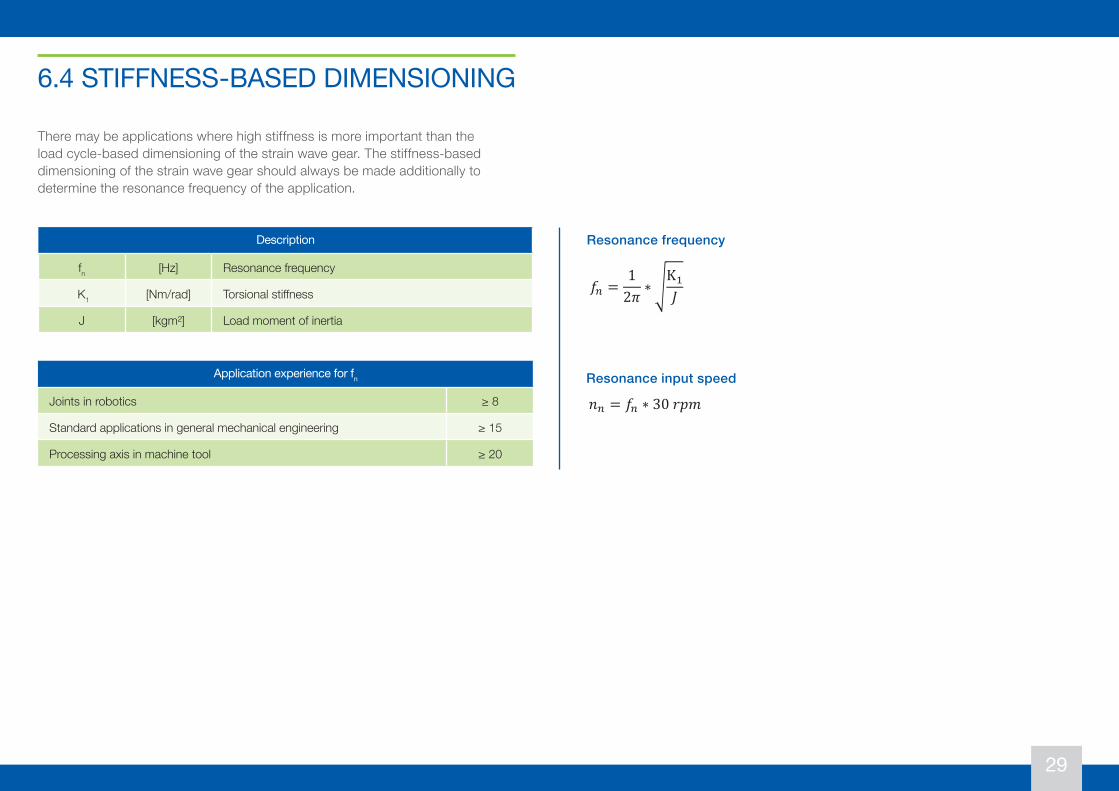
There may be applications where high stiffness is more important than the load cycle-based dimensioning of the strain wave gear. The stiffness-based dimensioning of the strain wave gear should always be made additionally to determine the resonance frequency of the application.

Resonance frequency

6.4 STIFFNESS-BASED DIMENSIONING

Description

fn [Hz] Resonance frequency

K1 [Nm/rad] Torsional stiffness

J [kgm²] Load moment of inertia

Resonance input speed Application experience for fn

Joints in robotics ≥ 8

Standard applications in general mechanical engineering ≥ 15

Processing axis in machine tool ≥ 20

30

6.4 Stiffness Based Dimensioning

There may be applications where high stiffness is more important than the load cycle based dimensioning of the strain wave gear. The stiffness based dimensioning of the strain wave gear should always be made additionally to determine the resonance frequency of the application.

Resonance frequency

𝑓𝑓* =12𝜋𝜋

∗ 1K'

𝐽𝐽

Resonance input speed 𝑛𝑛* = 𝑓𝑓* ∗ 30𝑟𝑟𝑟𝑟𝑟𝑟

Description fn [Hz] Resonance frequency K1 [Nm/rad] Torsional stiffness J [kgm²] Load moment of inertia

Application experience for fn Joints in robotics ≥ 8

Standard applications in general mechanical engineering ≥ 15 Processing axis in machine tool ≥ 20

30

6.4 Stiffness Based Dimensioning

There may be applications where high stiffness is more important than the load cycle based dimensioning of the strain wave gear. The stiffness based dimensioning of the strain wave gear should always be made additionally to determine the resonance frequency of the application.

Resonance frequency

𝑓𝑓* =12𝜋𝜋

∗ 1K'

𝐽𝐽

Resonance input speed 𝑛𝑛* = 𝑓𝑓* ∗ 30𝑟𝑟𝑟𝑟𝑟𝑟

Description fn [Hz] Resonance frequency K1 [Nm/rad] Torsional stiffness J [kgm²] Load moment of inertia

Application experience for fn Joints in robotics ≥ 8

Standard applications in general mechanical engineering ≥ 15 Processing axis in machine tool ≥ 20

30

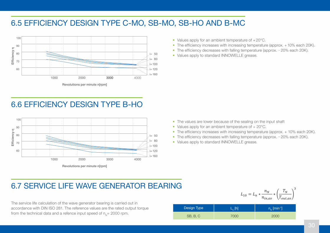
• Values apply for an ambient temperature of + 20°C.• The efficiency increases with increasing temperature (approx. + 10% each 20K).• The efficiency decreases with falling temperature (approx. − 20% each 20K).• Values apply to standard INNOWELLE grease.

6.5 EFFICIENCY DESIGN TYPE C-MO, SB-MO, SB-HO AND B-MC

6.6 EFFICIENCY DESIGN TYPE B-HO

• The values are lower because of the sealing on the input shaft • Values apply for an ambient temperature of + 20°C.• The efficiency increases with increasing temperature (approx. + 10% each 20K).• The efficiency decreases with falling temperature (approx. − 20% each 20K).• Values apply to standard INNOWELLE grease.

Revolutions per minute n[rpm]

100

90

80

70

60

1000 2000 3000 4000

Effic

ienc

y η

Revolutions per minute n[rpm]

100

90

80

70

60

1000 2000 3000 4000

Effic

ienc

y η

The service life calculation of the wave generator bearing is carried out in accordance with DIN ISO 281. The reference values are the rated output torque from the technical data and a refence input speed of nN= 2000 rpm.

6.7 SERVICE LIFE WAVE GENERATOR BEARING

Design Type Ln [h] nN [min-1]

SB, B, C 7000 2000

32

6.7 Service Life Wave Generator Bearing

The service life calculation of the wave generator bearing is carried out in accordance with DIN ISO 281. The reference values are the rated output torque from the technical data and a refence input speed of 𝑛𝑛5 = 2000𝑟𝑟𝑟𝑟𝑟𝑟.


𝑛𝑛-*,%&∗ ?

𝑇𝑇5𝑇𝑇!"#,%&

@(

6.8 Service Life Output Bearing

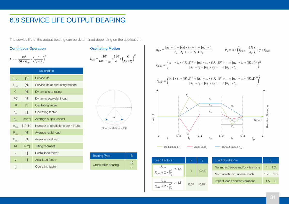
The service life of the output bearing can be determined depending on the application.

Continuous Operation Oscillating Motion

Description

L10 [h] Service life LOC [h] Service life at oscillating motion C [N] Dynamic load rating

PC [N] Dynamic equivalent load ϕ [°] Oscillating angle fw [ ] Operating factor nav [min-1] Average output speed nOC [1/min] Number of oscillations per minute

Fr,av [N] Average radial load

Fa,av [N] Average axial load

M [Nm] Tilting moment x [ ] Radial load factor y [ ] Axial load factor fW Operating factor

Design Type Ln [h] nN [min-1] SB, B, C 7500 2000

𝐿𝐿"# =10$

60 ∗ 𝑛𝑛%&∗ (

𝐶𝐶𝑓𝑓' ∗ 𝑃𝑃(

,)

𝐿𝐿*+ =10$

60 ∗ 𝑛𝑛*+∗180𝜑𝜑 ∗ (


,)

𝑛𝑛%& =|𝑛𝑛"| ∗ 𝑡𝑡" + |𝑛𝑛,| ∗ 𝑡𝑡, +⋯+ |𝑛𝑛-| ∗ 𝑡𝑡-

𝑡𝑡" + 𝑡𝑡, +⋯+ 𝑡𝑡- + 𝑡𝑡.

Bearing Type B

Cross roller bearing103

𝑃𝑃+ = 𝑥𝑥 ∗ 5𝐹𝐹/,%& +2𝑀𝑀𝑑𝑑.

: + 𝑦𝑦 ∗ 𝐹𝐹%,%&

One oscillation = 2 ϕ

i= 50i= 80i= 100i= 120i= 160

i= 50i= 80i= 100i= 120i= 160

31


6.8 SERVICE LIFE OUTPUT BEARING


One oscillation = 2φ

Bearing Type B


φ

Fr3

tp t1

n1

n2

n3

Time t

Rot

atio

n Sp

eed

n

Load

F

t2 t3 tp

Fr2

Fr1

Fa2

Fa2

Fa1

━━ Radial Load Fr ━━ Axial Loada ━━ Output Speed nout

32




𝑛𝑛-*,%&∗ ?

𝑇𝑇5𝑇𝑇!"#,%&

@(




Description







𝐿𝐿"# =10$

60 ∗ 𝑛𝑛%&∗ (


,)

𝐿𝐿*+ =10$

60 ∗ 𝑛𝑛*+∗180𝜑𝜑 ∗ (


,)

𝑛𝑛%& =|𝑛𝑛"| ∗ 𝑡𝑡" + |𝑛𝑛,| ∗ 𝑡𝑡, +⋯+ |𝑛𝑛-| ∗ 𝑡𝑡-

𝑡𝑡" + 𝑡𝑡, +⋯+ 𝑡𝑡- + 𝑡𝑡.

Bearing Type B


𝑃𝑃+ = 𝑥𝑥 ∗ 5𝐹𝐹/,%& +2𝑀𝑀𝑑𝑑.

: + 𝑦𝑦 ∗ 𝐹𝐹%,%&


32




𝑛𝑛-*,%&∗ ?

𝑇𝑇5𝑇𝑇!"#,%&

@(




Description







𝐿𝐿"# =10$

60 ∗ 𝑛𝑛%&∗ (


,)

𝐿𝐿*+ =10$

60 ∗ 𝑛𝑛*+∗180𝜑𝜑 ∗ (


,)

𝑛𝑛%& =|𝑛𝑛"| ∗ 𝑡𝑡" + |𝑛𝑛,| ∗ 𝑡𝑡, +⋯+ |𝑛𝑛-| ∗ 𝑡𝑡-

𝑡𝑡" + 𝑡𝑡, +⋯+ 𝑡𝑡- + 𝑡𝑡.

Bearing Type B


𝑃𝑃+ = 𝑥𝑥 ∗ 5𝐹𝐹/,%& +2𝑀𝑀𝑑𝑑.

: + 𝑦𝑦 ∗ 𝐹𝐹%,%&


32




𝑛𝑛-*,%&∗ ?

𝑇𝑇5𝑇𝑇!"#,%&

@(




Description







𝐿𝐿"# =10$

60 ∗ 𝑛𝑛%&∗ (


,)

𝐿𝐿*+ =10$

60 ∗ 𝑛𝑛*+∗180𝜑𝜑 ∗ (


,)

𝑛𝑛%& =|𝑛𝑛"| ∗ 𝑡𝑡" + |𝑛𝑛,| ∗ 𝑡𝑡, +⋯+ |𝑛𝑛-| ∗ 𝑡𝑡-

𝑡𝑡" + 𝑡𝑡, +⋯+ 𝑡𝑡- + 𝑡𝑡.

Bearing Type B


𝑃𝑃+ = 𝑥𝑥 ∗ 5𝐹𝐹/,%& +2𝑀𝑀𝑑𝑑.

: + 𝑦𝑦 ∗ 𝐹𝐹%,%&


33

6.9 Permissible Static Tilting Moment

In case of a static load, the bearing load capacity and the angle of inclination can be determined as follows.

Load factors x y

𝐹𝐹!,!#

𝐹𝐹$,!# + 2 ∗ 𝑀𝑀𝑑𝑑%

≤ 1,5 1 0,45

𝐹𝐹!,!#

𝐹𝐹$,!# + 2 ∗ 𝑀𝑀𝑑𝑑%

> 1,5 0,67 0,67

Load conditions fW No impact loads and/or vibrations 1 … 1,2

Normal rotation, normal loads 1,2 … 1,5 Impact loads and/or vibrations 1,5 … 3

Description fs [] Static load safety factor C0 [N] Static load rating Fr [N] Radial load Fa [N] Axial load x0 [] 1 y0 [] 0.45 P0 [1/min] Static equivalent load

dp [mm] Pitch circle diameter

𝛾𝛾 [arcmin] Angle of inclination at the output bearing

M [Nm] Tilting moment at the output bearing

M0 [Nm] Permissible static tilting moment

KB [Nm/arcmin] Radial load factor

Rotation condition for bearing fs

Normal 1 … 2 Impacts / Vibrations 2 … 3

High transmission accuracy ≥ 3

𝐹𝐹%,%& = 5|𝑛𝑛"| ∗ 𝑡𝑡" ∗ (|𝐹𝐹%"|)) + |𝑛𝑛,| ∗ 𝑡𝑡, ∗ (|𝐹𝐹%,|)) +⋯+ |𝑛𝑛-| ∗ 𝑡𝑡- ∗ (|𝐹𝐹%-|))

|𝑛𝑛"| ∗ 𝑡𝑡" + |𝑛𝑛,| ∗ 𝑡𝑡, +⋯+ |𝑛𝑛-| ∗ 𝑡𝑡-:

")

𝐹𝐹/,%& = 5|𝑛𝑛"| ∗ 𝑡𝑡" ∗ (|𝐹𝐹/"|)) + |𝑛𝑛,| ∗ 𝑡𝑡, ∗ (|𝐹𝐹/,|)) +⋯+ |𝑛𝑛-| ∗ 𝑡𝑡- ∗ (|𝐹𝐹/-|))

|𝑛𝑛"| ∗ 𝑡𝑡" + |𝑛𝑛,| ∗ 𝑡𝑡, +⋯+ |𝑛𝑛-| ∗ 𝑡𝑡-:

")

Load

F

Time t

n1

n2

n3

Rot

atio

n S

peed

n

Fr1

Fr2

Fr3

Fa1

Fa2

Fa3

Radial Load Fr

Axial Load Fa

Output Speed nout

t1 t2 t3 tptp

𝑀𝑀 = 𝐹𝐹/ ∗ (𝐿𝐿/ + 𝑅𝑅) + 𝐹𝐹% ∗ 𝐿𝐿%

𝑓𝑓1 =𝐶𝐶#𝑃𝑃# 𝑃𝑃# = 𝑥𝑥# ∗ 5𝐹𝐹/ +

2𝑀𝑀𝑑𝑑.

: + 𝑦𝑦# ∗ 𝐹𝐹%

𝑀𝑀# =𝑑𝑑. ∗ 𝐶𝐶#2 ∗ 𝑓𝑓1

𝛾𝛾 =𝑀𝑀𝐾𝐾)

32




𝑛𝑛-*,%&∗ ?

𝑇𝑇5𝑇𝑇!"#,%&

@(




Description







𝐿𝐿"# =10$

60 ∗ 𝑛𝑛%&∗ (


,)

𝐿𝐿*+ =10$

60 ∗ 𝑛𝑛*+∗180𝜑𝜑 ∗ (


,)

𝑛𝑛%& =|𝑛𝑛"| ∗ 𝑡𝑡" + |𝑛𝑛,| ∗ 𝑡𝑡, +⋯+ |𝑛𝑛-| ∗ 𝑡𝑡-

𝑡𝑡" + 𝑡𝑡, +⋯+ 𝑡𝑡- + 𝑡𝑡.

Bearing Type B


𝑃𝑃+ = 𝑥𝑥 ∗ 5𝐹𝐹/,%& +2𝑀𝑀𝑑𝑑.

: + 𝑦𝑦 ∗ 𝐹𝐹%,%&


φ

Description

L10 [h] Service life

LOC [N] Service life at oscillating motion

C [N] Dynamic load rating

PC [N] Dynamic equivalent load

φ [°] Oscillating angle

fw [ ] Operating factor

nav [min-1] Average output speed

nOC [1/min] Number of oscillations per minute



M [Nm] Tilting moment

x [ ] Radial load factor

y [ ] Axial load factor

fw Operating factor

Load Factors x y

1 0.45

0.67 0.67

Load Conditions fw

No impact loads and/or vibrations 1 …1.2

Normal rotation, normal loads 1.2 … 1.5

Impact loads and/or vibrations 1.5 … 3

33



Load factors x y

𝐹𝐹!,!#

𝐹𝐹$,!# + 2 ∗ 𝑀𝑀𝑑𝑑%

≤ 1,5 1 0,45

𝐹𝐹!,!#

𝐹𝐹$,!# + 2 ∗ 𝑀𝑀𝑑𝑑%

> 1,5 0,67 0,67













|𝑛𝑛"| ∗ 𝑡𝑡" + |𝑛𝑛,| ∗ 𝑡𝑡, +⋯+ |𝑛𝑛-| ∗ 𝑡𝑡-:

")


|𝑛𝑛"| ∗ 𝑡𝑡" + |𝑛𝑛,| ∗ 𝑡𝑡, +⋯+ |𝑛𝑛-| ∗ 𝑡𝑡-:

")

Load

F

Time t

n1

n2

n3

Rot

atio

n S

peed

n

Fr1

Fr2

Fr3

Fa1

Fa2

Fa3

Radial Load Fr

Axial Load Fa

Output Speed nout

t1 t2 t3 tptp

𝑀𝑀 = 𝐹𝐹/ ∗ (𝐿𝐿/ + 𝑅𝑅) + 𝐹𝐹% ∗ 𝐿𝐿%


2𝑀𝑀𝑑𝑑.

: + 𝑦𝑦# ∗ 𝐹𝐹%

𝑀𝑀# =𝑑𝑑. ∗ 𝐶𝐶#2 ∗ 𝑓𝑓1


33



Load factors x y

𝐹𝐹!,!#

𝐹𝐹$,!# + 2 ∗ 𝑀𝑀𝑑𝑑%

≤ 1,5 1 0,45

𝐹𝐹!,!#

𝐹𝐹$,!# + 2 ∗ 𝑀𝑀𝑑𝑑%

> 1,5 0,67 0,67













|𝑛𝑛"| ∗ 𝑡𝑡" + |𝑛𝑛,| ∗ 𝑡𝑡, +⋯+ |𝑛𝑛-| ∗ 𝑡𝑡-:

")


|𝑛𝑛"| ∗ 𝑡𝑡" + |𝑛𝑛,| ∗ 𝑡𝑡, +⋯+ |𝑛𝑛-| ∗ 𝑡𝑡-:

")

Load

F

Time t

n1

n2

n3

Rot

atio

n S

peed

n

Fr1

Fr2

Fr3

Fa1

Fa2

Fa3

Radial Load Fr

Axial Load Fa

Output Speed nout

t1 t2 t3 tptp

𝑀𝑀 = 𝐹𝐹/ ∗ (𝐿𝐿/ + 𝑅𝑅) + 𝐹𝐹% ∗ 𝐿𝐿%


2𝑀𝑀𝑑𝑑.

: + 𝑦𝑦# ∗ 𝐹𝐹%

𝑀𝑀# =𝑑𝑑. ∗ 𝐶𝐶#2 ∗ 𝑓𝑓1


32

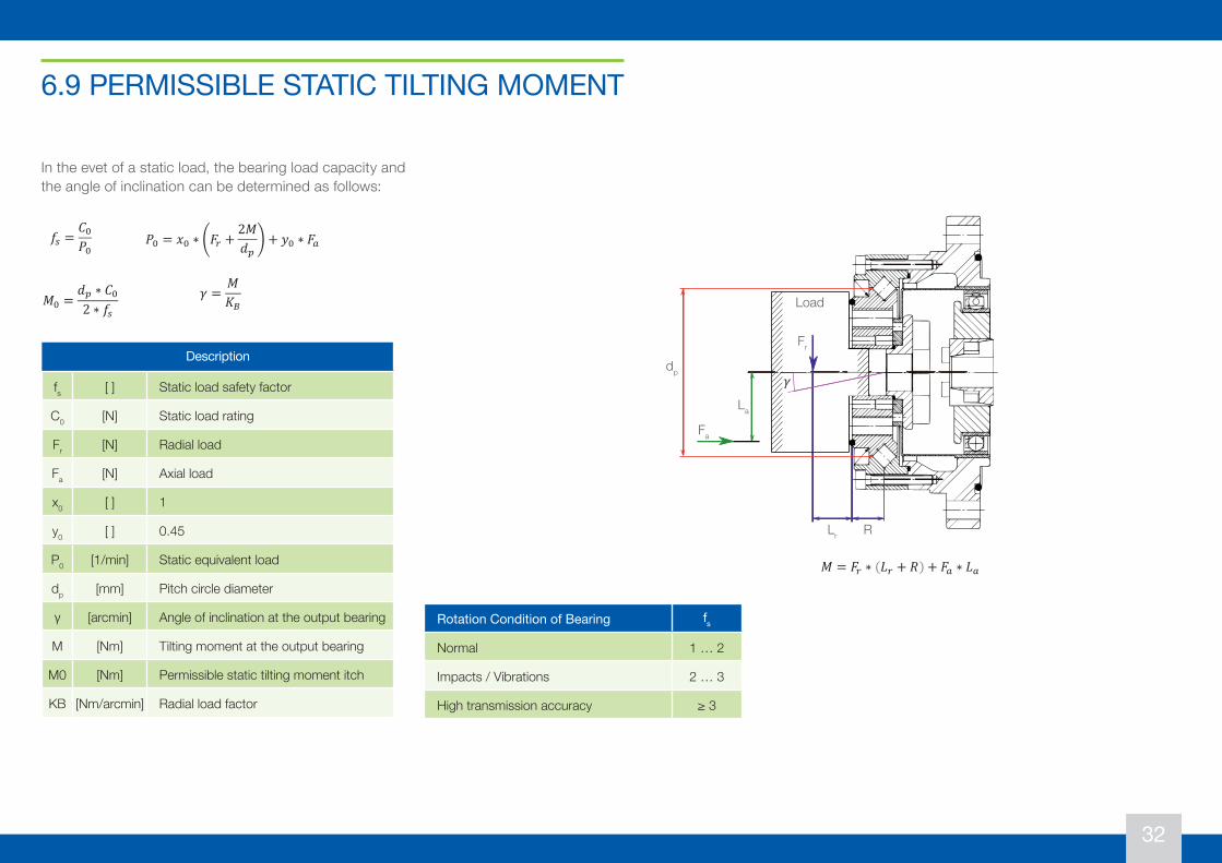
6.9 PERMISSIBLE STATIC TILTING MOMENT

In the evet of a static load, the bearing load capacity and the angle of inclination can be determined as follows:

Description

fs [ ] Static load safety factor

C0 [N] Static load rating

Fr [N] Radial load

Fa [N] Axial load

x0 [ ] 1

y0 [ ] 0.45

P0 [1/min] Static equivalent load


γ [arcmin] Angle of inclination at the output bearing


M0 [Nm] Permissible static tilting moment itch


Rotation Condition of Bearing fs

Normal 1 … 2

Impacts / Vibrations 2 … 3


33



Load factors x y

𝐹𝐹!,!#

𝐹𝐹$,!# + 2 ∗ 𝑀𝑀𝑑𝑑%

≤ 1,5 1 0,45

𝐹𝐹!,!#

𝐹𝐹$,!# + 2 ∗ 𝑀𝑀𝑑𝑑%

> 1,5 0,67 0,67













|𝑛𝑛"| ∗ 𝑡𝑡" + |𝑛𝑛,| ∗ 𝑡𝑡, +⋯+ |𝑛𝑛-| ∗ 𝑡𝑡-:

")


|𝑛𝑛"| ∗ 𝑡𝑡" + |𝑛𝑛,| ∗ 𝑡𝑡, +⋯+ |𝑛𝑛-| ∗ 𝑡𝑡-:

")

Load

F

Time t

n1

n2

n3

Rot

atio

n S

peed

n

Fr1

Fr2

Fr3

Fa1

Fa2

Fa3

Radial Load Fr

Axial Load Fa

Output Speed nout

t1 t2 t3 tptp

𝑀𝑀 = 𝐹𝐹/ ∗ (𝐿𝐿/ + 𝑅𝑅) + 𝐹𝐹% ∗ 𝐿𝐿%


2𝑀𝑀𝑑𝑑.

: + 𝑦𝑦# ∗ 𝐹𝐹%

𝑀𝑀# =𝑑𝑑. ∗ 𝐶𝐶#2 ∗ 𝑓𝑓1


33



Load factors x y

𝐹𝐹!,!#

𝐹𝐹$,!# + 2 ∗ 𝑀𝑀𝑑𝑑%

≤ 1,5 1 0,45

𝐹𝐹!,!#

𝐹𝐹$,!# + 2 ∗ 𝑀𝑀𝑑𝑑%

> 1,5 0,67 0,67













|𝑛𝑛"| ∗ 𝑡𝑡" + |𝑛𝑛,| ∗ 𝑡𝑡, +⋯+ |𝑛𝑛-| ∗ 𝑡𝑡-:

")


|𝑛𝑛"| ∗ 𝑡𝑡" + |𝑛𝑛,| ∗ 𝑡𝑡, +⋯+ |𝑛𝑛-| ∗ 𝑡𝑡-:

")

Load

F

Time t

n1

n2

n3

Rot

atio

n S

peed

n

Fr1

Fr2

Fr3

Fa1

Fa2

Fa3

Radial Load Fr

Axial Load Fa

Output Speed nout

t1 t2 t3 tptp

𝑀𝑀 = 𝐹𝐹/ ∗ (𝐿𝐿/ + 𝑅𝑅) + 𝐹𝐹% ∗ 𝐿𝐿%


2𝑀𝑀𝑑𝑑.

: + 𝑦𝑦# ∗ 𝐹𝐹%

𝑀𝑀# =𝑑𝑑. ∗ 𝐶𝐶#2 ∗ 𝑓𝑓1


33



Load factors x y

𝐹𝐹!,!#

𝐹𝐹$,!# + 2 ∗ 𝑀𝑀𝑑𝑑%

≤ 1,5 1 0,45

𝐹𝐹!,!#

𝐹𝐹$,!# + 2 ∗ 𝑀𝑀𝑑𝑑%

> 1,5 0,67 0,67













|𝑛𝑛"| ∗ 𝑡𝑡" + |𝑛𝑛,| ∗ 𝑡𝑡, +⋯+ |𝑛𝑛-| ∗ 𝑡𝑡-:

")


|𝑛𝑛"| ∗ 𝑡𝑡" + |𝑛𝑛,| ∗ 𝑡𝑡, +⋯+ |𝑛𝑛-| ∗ 𝑡𝑡-:

")

Load

F

Time t

n1

n2

n3

Rot

atio

n S

peed

n

Fr1

Fr2

Fr3

Fa1

Fa2

Fa3

Radial Load Fr

Axial Load Fa

Output Speed nout

t1 t2 t3 tptp

𝑀𝑀 = 𝐹𝐹/ ∗ (𝐿𝐿/ + 𝑅𝑅) + 𝐹𝐹% ∗ 𝐿𝐿%


2𝑀𝑀𝑑𝑑.

: + 𝑦𝑦# ∗ 𝐹𝐹%

𝑀𝑀# =𝑑𝑑. ∗ 𝐶𝐶#2 ∗ 𝑓𝑓1


33



Load factors x y

𝐹𝐹!,!#

𝐹𝐹$,!# + 2 ∗ 𝑀𝑀𝑑𝑑%

≤ 1,5 1 0,45

𝐹𝐹!,!#

𝐹𝐹$,!# + 2 ∗ 𝑀𝑀𝑑𝑑%

> 1,5 0,67 0,67













|𝑛𝑛"| ∗ 𝑡𝑡" + |𝑛𝑛,| ∗ 𝑡𝑡, +⋯+ |𝑛𝑛-| ∗ 𝑡𝑡-:

")


|𝑛𝑛"| ∗ 𝑡𝑡" + |𝑛𝑛,| ∗ 𝑡𝑡, +⋯+ |𝑛𝑛-| ∗ 𝑡𝑡-:

")

Load

F

Time t

n1

n2

n3

Rot

atio

n S

peed

n

Fr1

Fr2

Fr3

Fa1

Fa2

Fa3

Radial Load Fr

Axial Load Fa

Output Speed nout

t1 t2 t3 tptp

𝑀𝑀 = 𝐹𝐹/ ∗ (𝐿𝐿/ + 𝑅𝑅) + 𝐹𝐹% ∗ 𝐿𝐿%


2𝑀𝑀𝑑𝑑.

: + 𝑦𝑦# ∗ 𝐹𝐹%

𝑀𝑀# =𝑑𝑑. ∗ 𝐶𝐶#2 ∗ 𝑓𝑓1


Load

dp

Fa

La

Fr

Lr R

33

6.10 CALCULATION OF THE TORSIONAL ANGLE

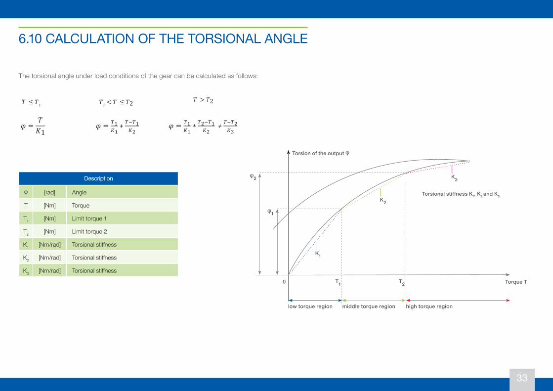
The torsional angle under load conditions of the gear can be calculated as follows:

Description

φ [rad] Angle

T [Nm] Torque

T1 [Nm] Limit torque 1

T2 [Nm] Limit torque 2




Torque TT2

Torsion of the output φ

Torsional stiffness K1, K2 and K3

low torque region middle torque region high torque region

K3

K2

K1

T10

φ1

φ2

34

6.10 Calculation of the Torsional Angle The torsional angle under load conditions of the gear can be calculated as follows.

Description

ϕ [rad] Angle T [Nm] Torque T1 [Nm] Limit torque 1 T2 [Nm] Limit torque 2 K1 [Nm/rad] Torsional stiffness K2 [Nm/rad] Torsional stiffness K3 [Nm/rad] Torsional stiffness

𝑇𝑇 ≤ 𝑇𝑇1 𝑇𝑇1 < 𝑇𝑇 ≤ 𝑇𝑇2 𝑇𝑇 > 𝑇𝑇2

𝜑𝜑 =𝑇𝑇𝐾𝐾1

𝜑𝜑 = B'3'

+ BCB'3)

𝜑𝜑 = B'3'

+ B)CB'3)

+ BCB)3(

Torsion of the output

Torque T

1

2

T1 T2

ϕ

ϕ

ϕ

K1

K2

K3


0


34

6.10 Calculation of the Torsional Angle The torsional angle under load conditions of the gear can be calculated as follows.

Description

ϕ [rad] Angle T [Nm] Torque T1 [Nm] Limit torque 1 T2 [Nm] Limit torque 2 K1 [Nm/rad] Torsional stiffness K2 [Nm/rad] Torsional stiffness K3 [Nm/rad] Torsional stiffness

𝑇𝑇 ≤ 𝑇𝑇1 𝑇𝑇1 < 𝑇𝑇 ≤ 𝑇𝑇2 𝑇𝑇 > 𝑇𝑇2

𝜑𝜑 =𝑇𝑇𝐾𝐾1

𝜑𝜑 = B'3'

+ BCB'3)

𝜑𝜑 = B'3'

+ B)CB'3)

+ BCB)3(

Torsion of the output

Torque T

1

2

T1 T2

ϕ

ϕ

ϕ

K1

K2

K3


0


34

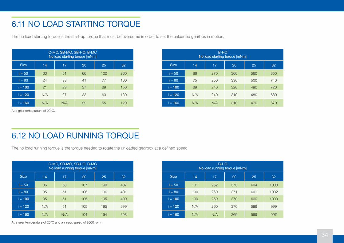
C-MC, SB-MO, SB-HO, B-MCNo load starting torque [mNm]

Size 14 17 20 25 32

i = 50 33 51 66 120 260

i = 80 24 33 41 77 160

i = 100 21 29 37 69 150

i = 120 N/A 27 33 63 130

i = 160 N/A N/A 29 55 120

C-MC, SB-MO, SB-HO, B-MCNo load running torque [mNm]

Size 14 17 20 25 32

i = 50 36 53 107 199 407

i = 80 35 51 106 196 401

i = 100 35 51 105 195 400

i = 120 N/A 51 105 195 399

i = 160 N/A N/A 104 194 398

B-HONo load starting torque [mNm]

Size 14 17 20 25 32

i = 50 88 270 360 560 850

i = 80 75 250 330 500 740

i = 100 69 240 320 490 720

i = 120 N/A 240 310 480 680

i = 160 N/A N/A 310 470 670

B-HONo load running torque [mNm]

Size 14 17 20 25 32

i = 50 101 262 373 604 1008

i = 80 100 260 371 601 1002

i = 100 100 260 370 600 1000

i = 120 N/A 260 370 599 999

i = 160 N/A N/A 369 599 997

6.11 NO LOAD STARTING TORQUE

6.12 NO LOAD RUNNING TORQUE

The no load starting torque is the start-up torque that must be overcome in order to set the unloaded gearbox in motion.

The no load running torque is the torque needed to rotate the unloaded gearbox at a defined speed.

At a gear temperature of 20°C.

At a gear temperature of 20°C and an input speed of 2000 rpm.

35

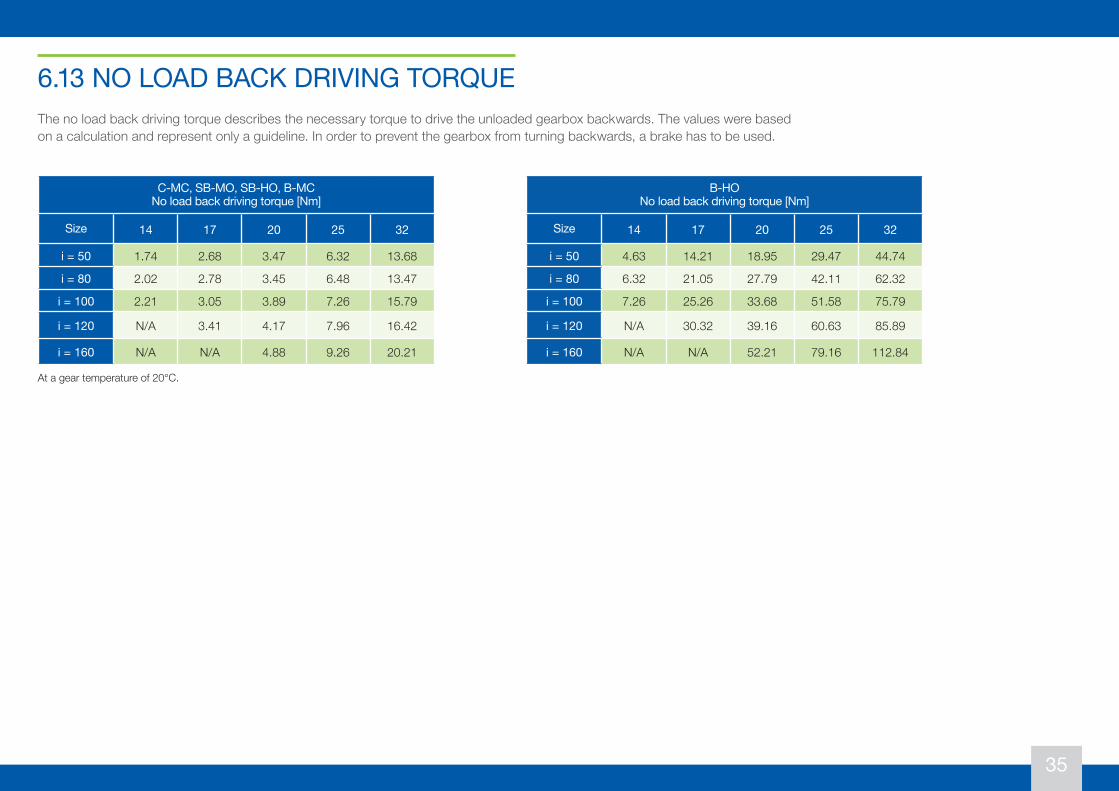
C-MC, SB-MO, SB-HO, B-MCNo load back driving torque [Nm]

Size 14 17 20 25 32

i = 50 1.74 2.68 3.47 6.32 13.68

i = 80 2.02 2.78 3.45 6.48 13.47

i = 100 2.21 3.05 3.89 7.26 15.79

i = 120 N/A 3.41 4.17 7.96 16.42

i = 160 N/A N/A 4.88 9.26 20.21

B-HONo load back driving torque [Nm]

Size 14 17 20 25 32

i = 50 4.63 14.21 18.95 29.47 44.74

i = 80 6.32 21.05 27.79 42.11 62.32

i = 100 7.26 25.26 33.68 51.58 75.79

i = 120 N/A 30.32 39.16 60.63 85.89

i = 160 N/A N/A 52.21 79.16 112.84

6.13 NO LOAD BACK DRIVING TORQUEThe no load back driving torque describes the necessary torque to drive the unloaded gearbox backwards. The values were based on a calculation and represent only a guideline. In order to prevent the gearbox from turning backwards, a brake has to be used.

At a gear temperature of 20°C.

36

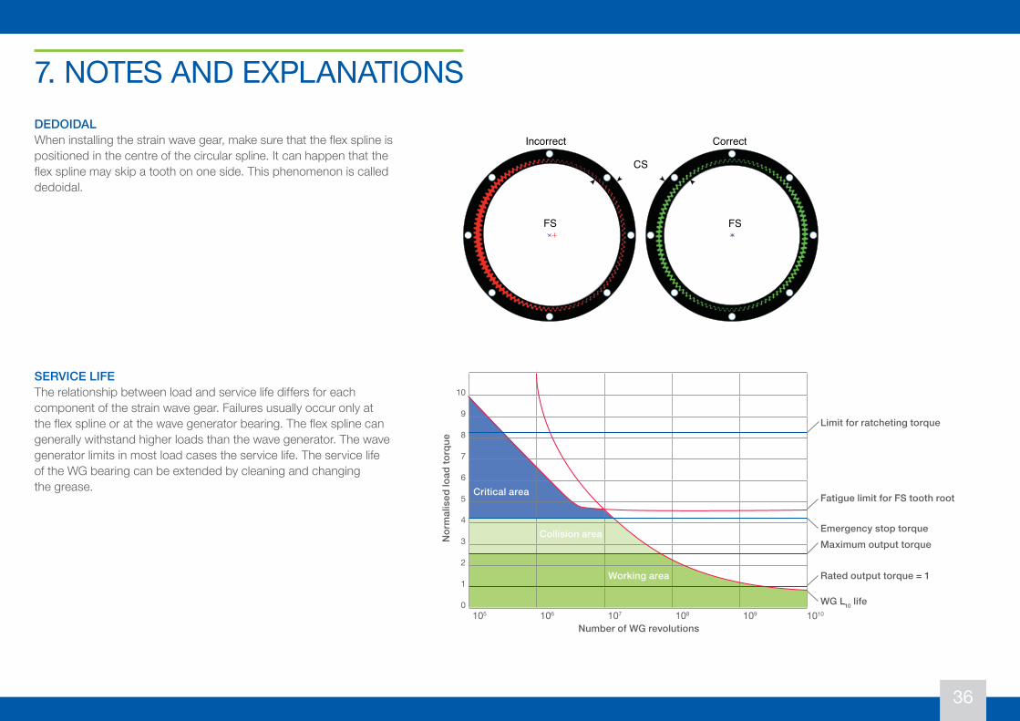
7. NOTES AND EXPLANATIONSDEDOIDALWhen installing the strain wave gear, make sure that the flex spline is positioned in the centre of the circular spline. It can happen that the flex spline may skip a tooth on one side. This phenomenon is called dedoidal.

SERVICE LIFEThe relationship between load and service life differs for each component of the strain wave gear. Failures usually occur only at the flex spline or at the wave generator bearing. The flex spline can generally withstand higher loads than the wave generator. The wave generator limits in most load cases the service life. The service life of the WG bearing can be extended by cleaning and changing the grease.

10

9

8

7

6

5

4

3

2

1

0105 106 107 108 109

Nor

mal

ised

load

torq

ue

1010

Fatigue limit for FS tooth root

Emergency stop torqueMaximum output torque

Rated output torque = 1

WG L10 life

Limit for ratcheting torque

Number of WG revolutions

Critical area

Collision area

Working area

CorrectIncorrect

CS

FS FS

37

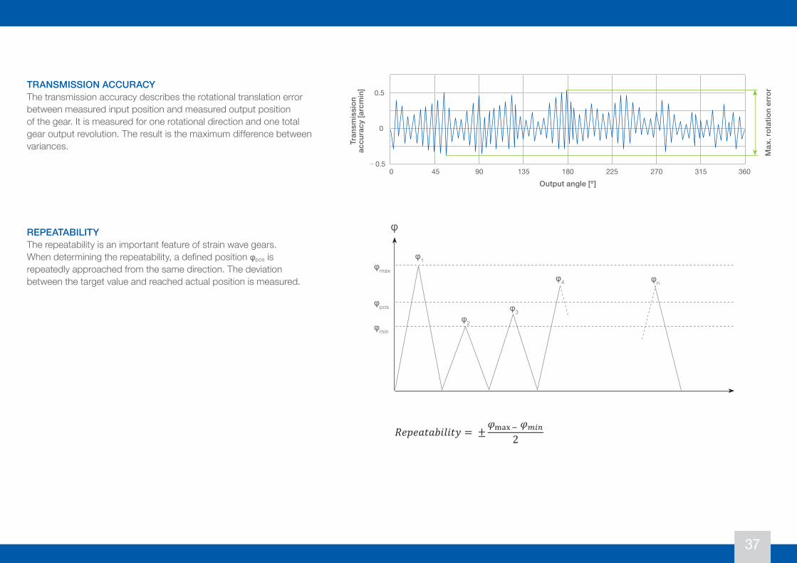
TRANSMISSION ACCURACYThe transmission accuracy describes the rotational translation error between measured input position and measured output position of the gear. It is measured for one rotational direction and one total gear output revolution. The result is the maximum difference between variances.

REPEATABILITYThe repeatability is an important feature of strain wave gears. When determining the repeatability, a defined position φpos is repeatedly approached from the same direction. The deviation between the target value and reached actual position is measured.

Tran

smis

sion

ac

cura

cy [a

rcm

in]

0 45 90 135 180 225 270 315 360

0.5

0

− 0.5

Output angle [º]

Max

. rot

atio

n er

ror

φ1

φ2

φ3

φ4 φn

φmax

φpos

φmin

φ

38

Transmission Accuracy The transmission accuracy describes the rotational translation error between measured input position and measured output position of the gear. It is measured for one rotational direction and one total gear output revolution. The result is the maximum difference between variances.

Repeatability The Repeatability is an important feature of strain wave gears. When determining the repeatability, a defined position jpos is repeatedly approached from the same direction. The deviation between the target value and reached actual position is measured.

𝑅𝑅𝑅𝑅𝑅𝑅𝑅𝑅𝑅𝑅𝑅𝑅𝑅𝑅𝑅𝑅𝑅𝑅𝑅𝑅𝑅𝑅𝑅𝑅𝑅𝑅 = ±𝜑𝜑DEFC𝜑𝜑/-*

2

Hysteresis Loss The torsional torque diagram of a strain wave gear has the typical characteristic of a hysteresis curve. The hysteresis curve typically does not pass through the coordinate origin. The angle deviation at zero torque is called hysteresis loss.

45 90

0

Output angle[°]

Tran

smiss

ion ac

cura

cy [a

rcmi

n]

0 135 180 225 270 315 360

Max

. rot

ation

erro

r

0,5

-0,5

𝜑𝜑

𝜑𝜑max

𝜑𝜑pos

𝜑𝜑min

𝜑𝜑1

𝜑𝜑2

𝜑𝜑3

𝜑𝜑4 𝜑𝜑n

Rotation angle

Torque T

Hysteresis Loss

38

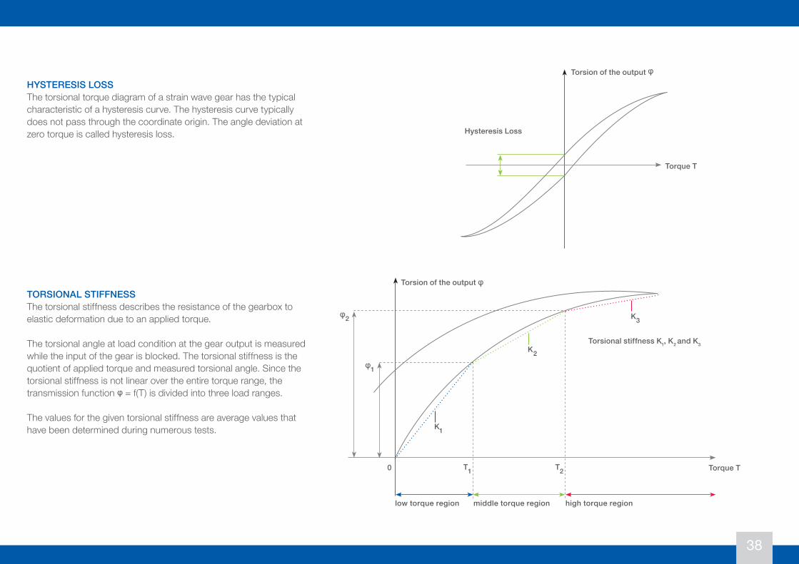
HYSTERESIS LOSSThe torsional torque diagram of a strain wave gear has the typical characteristic of a hysteresis curve. The hysteresis curve typically does not pass through the coordinate origin. The angle deviation at zero torque is called hysteresis loss.

TORSIONAL STIFFNESSThe torsional stiffness describes the resistance of the gearbox to elastic deformation due to an applied torque.

The torsional angle at load condition at the gear output is measured while the input of the gear is blocked. The torsional stiffness is the quotient of applied torque and measured torsional angle. Since the torsional stiffness is not linear over the entire torque range, the transmission function φ = f(T) is divided into three load ranges.

The values for the given torsional stiffness are average values that have been determined during numerous tests.

Torque TT2




K3

K2

K1

T10

φ1

φ2

Torque T


Hysteresis Loss

39

COPYRIGHT Pictures, graphics and texts, including other contents as well as the layout of this document, are protected by copyright. All rights are owned by the owner or, insofar as graphics, photos, texts and contributions from other sources are used, by the respective authors. Any duplication or use of information and data, particularly the use of texts or parts of texts is not permitted without agreement.

DISCLAIMERThe descriptions, technical data and explanations in this catalogue have been compiled by us with the greatest care and attention. We reserve the right not to be responsible for the topicality, correctness, completeness or quality of the provided information.

8. COPYRIGHT AND DISCLAIMER

INNOWELLE GmbHHeidestrasse 235625 HüttenbergTel.: +49 6441 78 591 0

[email protected] KAT_V01 Date: 05/2021

Documents

DRIVE TECHNOLOGY ENGINEERED FOR ROBOTICS