451451

A. Bahari1 and A. Baradaran Seyed2

1 Iranian Central Oil Fields Company (ICOFC), Esfandiari St., Valiasr Ave., Tehran, Iran2 Behinkav Zharfa Consulting Engineers, No. 45, Block 18, Phase 2, Ekbatan, Tehran, Iran

Abstract: In drilling operation, a large saving in time and money would be achieved by reducing the drilling time, since some of the costs are time-dependent. Drilling time could be minimized by raising the penetration rate. In the comparative optimization method, by using the records of the fi rst drilled wells and comparing the criteria like penetration rate, cost per foot and specifi c energy, the drilling parameters of the next wells being drilled can be optimized in each depth interval. In the mathematical optimization technique, some numerical equations to model the penetration rate, bit wear rate and hydraulics would be used to minimize the drilling cost and time as much as possible and improve the results of the primary comparative optimization.

In this research, as a case study the Iranian Khangiran gas fi eld has been evaluated to optimize the drilling costs. A combination of the mentioned optimization techniques resulted in an optimal well which reduced the drilling time and cost considerably in comparison with the wells already drilled.

Key words: Optimization, cost per foot, penetration rate, drilling performance

Drilling cost optimization in a hydrocarbon fi eld by combination of comparative and mathematical methods

*Corresponding author. email: aboozar.bahari@Gmail.comReceived March 8, 2009

DOI: 10.1007/s12182-009-0069-xPet.Sci.(2009)6:451-463

1 IntroductionCost optimization is a procedure, and its final goal is

to reduce the cost by setting the interfering parameters to the optimum level. Optimization drilling techniques, first applied in 1967, have considerably reduced the drilling costs and currently have become an important aspect of drilling technology. The philosophy of optimization in drilling operation is using the record of the first drilled wells as a basis and applying optimization techniques to reduce drilling costs for the next wells being drilled (Lummus, 1970; 1971). In other words, by comparing the records of the fi rst drilled wells, the drilling variables will be gradually changed to their most effective level to reduce time and cost of drilling operation. In addition, the optimum procedures can also be applied in rig selection, to improve equipment life and well-bore stability and to reduce the drilling problems. It should be addressed that a large number of controllable and uncontrollable variables affect penetration rate and drilling cost. Recognizing and understanding those factors is obviously of prime importance. Controlled field studies are often the best way to understand the relationships between drilling factors under a set of conditions that are tightly controlled (Kaiser, 2007).

Up to now, many researchers have studied drilling optimization techniques and their application in hydrocarbon

fi elds. Several mathematical models that combine the known relationships of affecting parameters on rotary drilling process have been set up. For example, Rabia (1985) introduced the method of specific energy to select the optimal bit and enhance rock-cutting performance. Njobuenwu and wobo (2007) analyzed the results of laboratory investigations on the effect of drilled solids on drilling performance. Among the penetration rate models, the model proposed by Bourgoyne and Young (1974) is perhaps the most complete and widely accepted one. Eight functions are used in their equation to model the effect of most important drilling variables. In addition, they also proposed models of bit wear rate, optimum bit weight, and rotary speed.

In the recent years, the enhanced mathematical techniques have shown their capabilities of modeling the complex relationships in rotary drilling process. Bilgesu et al (1997) have applied neural networks to predict the penetration rate in petroleum wells. Bahari et al (2008) have proved that genetic algorithm is the most efficient mathematical technique to compute the constants of Bourgoyne-Young penetration rate model.

In this study, comparative and mathematical drilling optimization techniques are first described in detail. Then, they are employed to minimize the drilling time and cost for the next wells being drilled in Iranian Khangiran gas fi eld.

2 Comparative drilling optimization method Drilling optimization through comparison technique is

based on criteria such as cost per foot (Cf), specifi c energy (ES)

452

and penetration rate (R) to optimize the drilling variables. The drilling cost per foot is defi ned by the following formula:

DtttCC

C tcbrbf

)( … (1)

whereCf = Drilling cost per foot, $/ft, Cb = Cost of bit, $,Cr = Fixed operating cost of the rig per unit time,$/hr,ΔD = Drilled footage, ft,tb = Rotating time during the bit run, hr, tc = Non-rotating time during the bit run, hr, tt = Trip time, hr.

If the controllable drilling parameters are at the optimum level, the lowest cost per foot will be achieved. The most important controllable variables, affecting cost per foot and penetration rate are bit type, bit weight, rotary speed, mud properties, and bit hydraulics. It has long been observed that the penetration rate generally increases with increasing bit weight (W), rotary speed (N), bit hydraulic horsepower (PHb), fluid loss (L) and fractional bit tooth height. On the other hand, it decreases with increasing drilling fl uid viscosity, mud density (ρ) and fl uid solid content (S). Some of these variables may have significant effects on drilling rate whereas others may have marginal effects.

Specifi c Energy (ES) is defi ned as the energy required to remove a unit volume of rock. ES is a performance indicator for rock cutting and provides a means for selection of appropriate bit type since it is highly dependent on the type and design of bits. The following equation is suggested to compute ES (Rabia, 1985).

(2)Rd

WNES 20

whereES = specifi c energy, in.lb/in3,W = weight on Bit, lbf,N = rotary speed, rpm,d = hole diameter, in,R = rate of penetration, ft/hr.

If in the same depths of different drilled wells, geological condition is similar (i.e. formations are approximately horizontal and they are not very complicated), plotting a chart of controllable variables, cost per foot, penetration rate and specifi c energy, versus depth for each well makes it possible to determine the optimum variables values through comparison of the plotted charts. In other words, if the cost per foot and specifi c energy of a drilled well are lowest and its penetration rate is highest in a particular interval, the parameters values of that well and the bit type used, will be attributed to that considered interval. After determination of optimum drilling parameters and bit type for each depth interval, an optimized well would be obtained.

Since the footage of the drilled depth (ΔD), bit rotating time (tb) and trip time (tc+tt) are known in daily drilling progress reports, counting the price of the bits (Cb), and at-tributing an approximate price to the rig (Cr), the cost per foot can be computed from Eq. 1 for each drilling day of the

selected wells. Then, the chart of the cost per foot can be produced for each well.

It is wise to mention the fact that, the fi rst step in putting together an optimized drilling program should be to plan a detailed mud program in which the effect of mud parameters on many items, such as cuttings lifting capacity, penetration rate, hole stability, formation damage, lost circulation, pipe sticking and also controlling formation pressure, are considered. The procedure introduced in this section enables detection of changeable mud properties to increase penetration rate and decrease cost per foot without causing hole trouble. Therefore, the other criteria for selection of appropriate mud properties are neglected here and will be studied in other research.

3 Mathematical drilling optimization methodDrilling cost optimization through mathematical

techniques is based on the proposed models of the penetration rate, bit hydraulics, bit wear, etc, to predict and eventually optimize the rate of penetration and drilling cost. It should be noted that, the analytic results that are derived under field studies are often based on engineering and scientific principles and thus, the ability to generalize the results for other fi elds and locations may be limited (Kaiser, 2007).

Fig. 1 summarizes the algorithmic steps, which should be followed consecutively to optimize drilling parameters of a hydrocarbon fi eld using mathematical solutions. As shown in this fi gure, some of the comparative optimization results like selection of optimal bit and mud properties will be employed in the numerical technique. Each step of this algorithm will be described in detail while the case study is analyzed below.

Modellingpenetration rate

Hydraulicoptimization

Determining maximum allowablemechanical horsepower

Modelling wearrate of selected bits

Specifying optimum bitweight/rotary speed tominimize cost per foot

Optimumbit selection

Comparativeoptimization method

Optimum drillingmud properties

Data preparation and validation

Fig. 1 Algorithm of the mathematical optimization procedure

Pet.Sci.(2009)6:451-463

453

4 Application of drilling optimization techniques in Iranian Khangiran gas fi eld

4.1 Khangiran gas fi eldThe Khangiran gas fi eld is located in the northeast of Iran.

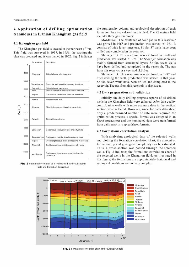
This field was surveyed in 1937. In 1956, the stratigraphy plan was prepared and it was named in 1962. Fig. 2 indicates

the stratigraphy column and geological description of each formation for a typical well in this fi eld. The Khangiran fi eld includes three gas reservoirs:

Mozdouran: The existence of sour gas in this reservoir was proved in 1968 and production was started in 1983. It consists of thick layer limestone. So far, 37 wells have been drilled and completed in the reservoir.

Shourijeh B: This reservoir was explored in 1968 and production was started in 1974. The Shourijeh formation was mainly formed from sandstone layers. So far, seven wells have been drilled and completed in the reservoir. The gas from this reservoir is sweet and H2S free.

Shourijeh D: This reservoir was explored in 1987 and after drilling the well, production was started in that year. So far, seven wells have been drilled and completed in the reservoir. The gas from this reservoir is also sweet.

4.2 Data preparation and validationInitially, the daily drilling progress reports of all drilled

wells in the Khangiran fi eld were gathered. After data quality control, nine wells with more accurate data in the vertical section were selected. However, since for each data sheet only a predetermined number of data were required for optimization process, a special format was designed in an Excel spreadsheet and the nominated data were transformed from daily reports to spreadsheet formats.

4.3 Formations correlation analysisWith analyzing geological data of the selected wells

and plotting the formation correlation chart, the amount of formation dip and geological complexity can be estimated. Thus, a cross section was passed through the selected wells. Fig. 3 indicates the formations correlation chart of the selected wells in the Khangiran field. As illustrated in this fi gure, the formations are approximately horizontal and geological conditions are not very complex.

Khangiran

Chehelkaman

PestehlighKalat

Neyzar

Abtalkh

Abderaz

Aytamir

Sanganeh

Sarcheshmeh

Tirgan

Shourijeh

Mozdouran

0

1000

2000

3000

4000

5000

6000

7000

8000

9000

10000

11000

Formations

Dep

th, f

t

Silty shale and silty claystone

Description

Dolomite and anhydrite to sandy limestone

M icritic to crystaline limestone and dolomiteSilty shale and sandstone

Calcareous sandstone, siltstone and shale

Silty shale and marl

M icritic limestone, silty calcareous shale

Glaconitic sandstone

Calcareous shale, claystone and silty shale

Argilaceous micritic limestone, some shale

Oolitic argilaceous micritic limestone, marl, shale

Oolitic sandstone and Calcareous silty shale

Argilaceous limestone and oolitic dolomite limestone

Fig. 2 Stratigraphy column of a typical well in the Khangiran fi eld and formation description

0 1 2 3 4 5 6 7 8 9 10x 104

-12000

-10000

-8000

-6000

-4000

-2000

0

2000

Distance, ft

Dep

th (m

ean

sea

leve

l), ft

Well 26Well 50 Well 42 Well 20 Well 28 Well 46 Well 29 Well 39

Well 47

Khangiran

PestehlighKalat Neyzar AbtalkhAbderazAytamirSanganehSarcheshmehTirgan

ShourijehMozdouran

Chehelkaman

Fig. 3 Formations correlation chart of the Khangiran fi eld

Pet.Sci.(2009)6:451-463

454

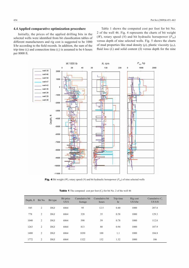
4.4 Applied comparative optimization procedure Initially, the prices of the applied drilling bits in the

selected wells were identifi ed from bit classifi cation tables of different manufacturers and rig cost is suggested to be 1000 $/hr according to the fi eld records. In addition, the sum of the trip time (tt) and connection time (tc) is assumed to be 6 hours per 8000 ft.

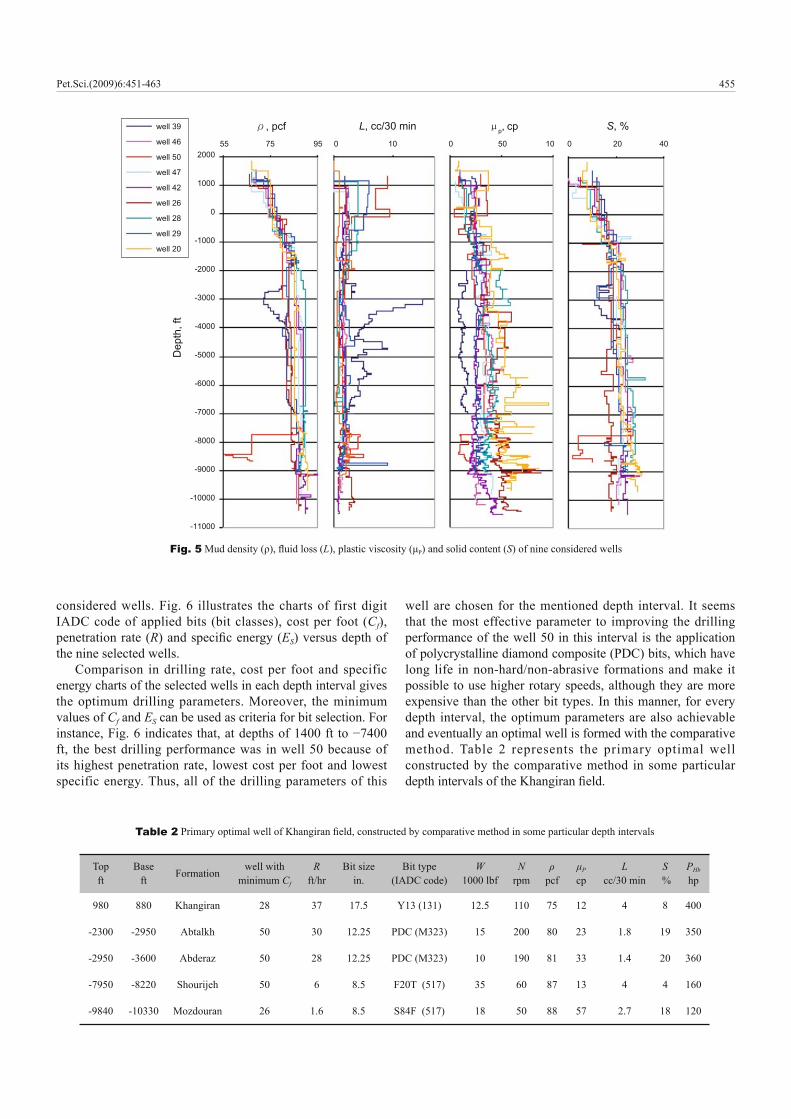
Table 1 shows the computed cost per foot for bit No. 2 of the well 46. Fig. 4 represents the charts of bit weight (W), rotary speed (N) and bit hydraulic horsepower (PHb) versus depth of nine selected wells. Fig. 5 shows the charts of mud properties like mud density (ρ), plastic viscosity (μP), fl uid loss (L) and solid content (S) versus depth for the nine

Fig. 4 Bit weight (W), rotary speed (N) and bit hydraulic horsepower (PHb) of nine selected wells

Depth, ft Bit No. Bit type Bit price US $

Cumulative bit footage

Cumulative bit hours

Trip time hr

Rig cost US $/hr

Cumulative Cf US $/ft

545 2 DGJ 6864 95 12.5 0.40 1000 207.8

778 2 DGJ 6864 328 35 0.58 1000 129.3

1040 2 DGJ 6864 590 59 0.78 1000 112.8

1263 2 DGJ 6864 813 80 0.94 1000 107.9

1480 2 DGJ 6864 1030 100 1.1 1000 104.8

1772 2 DGJ 6864 1322 132 1.32 1000 106

Table 1 The computed cost per foot (Cf) for bit No. 2 of the well 46

Pet.Sci.(2009)6:451-463

455

considered wells. Fig. 6 illustrates the charts of first digit IADC code of applied bits (bit classes), cost per foot (Cf), penetration rate (R) and specifi c energy (ES) versus depth of the nine selected wells.

Comparison in drilling rate, cost per foot and specific energy charts of the selected wells in each depth interval gives the optimum drilling parameters. Moreover, the minimum values of Cf and ES can be used as criteria for bit selection. For instance, Fig. 6 indicates that, at depths of 1400 ft to −7400 ft, the best drilling performance was in well 50 because of its highest penetration rate, lowest cost per foot and lowest specific energy. Thus, all of the drilling parameters of this

well are chosen for the mentioned depth interval. It seems that the most effective parameter to improving the drilling performance of the well 50 in this interval is the application of polycrystalline diamond composite (PDC) bits, which have long life in non-hard/non-abrasive formations and make it possible to use higher rotary speeds, although they are more expensive than the other bit types. In this manner, for every depth interval, the optimum parameters are also achievable and eventually an optimal well is formed with the comparative method. Table 2 represents the primary optimal well constructed by the comparative method in some particular depth intervals of the Khangiran fi eld.

well 39

well 46

well 50

well 47

well 42

well 26

well 28

well 29

well 20

2000

1000

0

-1000

-2000

-3000

-4000

-5000

-6000

-7000

-8000

-9000

-10000

-11000

Dep

th, f

t

ρ, pcf L, cc/30 min S, %55 75 95 0 10 50 10 0 20

p, cp0 40

Fig. 5 Mud density (ρ), fl uid loss (L), plastic viscosity (μP) and solid content (S) of nine considered wells

Topft

Base ft Formation well with

minimum Cf

R ft/hr

Bit size in.

Bit type(IADC code)

W 1000 lbf

N rpm

ρ pcf

μP cp

L cc/30 min

S %

PHb

hp

980 880 Khangiran 28 37 17.5 Y13 (131) 12.5 110 75 12 4 8 400

-2300 -2950 Abtalkh 50 30 12.25 PDC (M323) 15 200 80 23 1.8 19 350

-2950 -3600 Abderaz 50 28 12.25 PDC (M323) 10 190 81 33 1.4 20 360

-7950 -8220 Shourijeh 50 6 8.5 F20T (517) 35 60 87 13 4 4 160

-9840 -10330 Mozdouran 26 1.6 8.5 S84F (517) 18 50 88 57 2.7 18 120

Table 2 Primary optimal well of Khangiran fi eld, constructed by comparative method in some particular depth intervals

Pet.Sci.(2009)6:451-463

456

4.5 Applied mathematical optimization procedure To simplify the computation process in the mathematical

optimization procedure, the formations are regarded as homogeneous and their physical properties are considered constant throughout the entire depth interval to be drilled.4.5.1 Modeling the penetration rate

Up to now, several mathematical models that attempt to combine the relationships of drilling variables with penetration rate have been proposed. These models make it possible to apply mathematical optimization methods to the problem of selecting the best bit weight and rotary speed to achieve the minimum cost per foot.

Bourgoyne and Young (1974) have suggested the following equation to model the penetration rate when using roller cone bits:

(3a) 87654321 ffffffffR

The functional relations in this equation are:

Kef a1303.21 (3b)

(3c))10000(303.22

2 Daef

(3d) )9(303.23

69.03 pgDaef

(3e))(303.2

44 cpgDaef

(3f)

5

45

a

tb

tbb

dW

dW

dW

f

(3g)

6

606

aNf

haef 77 (3h)

8

10008

ajF

f (3i)

wherea1 to a8 = constants,D = true vertical depth, ft,db = bit diameter, in.,Fj = jet impact force, lbf ,gp = pore pressure gradient, lbm/gal, h = fractional bit tooth wear,ρc = equivalent circulating density, lbm/gal,N = rotary speed, rpm,R = rate of penetration, ft/hr, W = weight on bit, 1000 lbf

(W/db)t = threshold bit weight per inch of bit diameter at which the bit begins to drill, 1000 lbf/in.

well 46

well 47

well 39

well 50

well 42

well 29

well 28

well 26

well 20

Dep

th, (

sea

leve

l), ft

2000

1000

0

-1000

-2000

-3000

-4000

-5000

-6000

-7000

-8000

-9000

-10000

-11000

Bit class0 1 2 3 4 5 6 (PDC Bit)

D3well 50

well 28

well 47

well 46

well 42

well 39

well 29

well 26

well 20

2000

1000

0

-1000

-2000

-3000

-4000

-5000

-6000

-7000

-8000

-9000

-10000

-11000

Cf, $/ft200 4000

R, ft/hr500 20000

ES (1000 lb in/in3)

Fig. 6 First digit IADC code of applied bits (bit classes), cost per foot (Cf), penetration rate (R) and specifi c energy (ES) of the nine selected wells

Pet.Sci.(2009)6:451-463

457

The function f1 represents the effect of formation strength, bit type, mud type, and solid content, which are not included in the drilling model. This term is expressed in the same units as penetration rate and often is called the formation drillability. The functions f2 and f3 model the effect of compaction on penetration rate. The function f4 models the effect of overbalance on penetration rate. The functions f5 and f6 model the effect of bit weight and rotary speed on penetration rate. The function f7 models the effect of tooth wear and the function f8 models the effect of bit hydraulics on penetration rate.

The constants a1 to a8 are dependent on local drilling conditions and must be computed for each formation using the previous drilling data obtained in the area when detailed drilling data are available. In fact, the accuracy of this model is dependent to the coeffi cient values and therefore, applying a reliable mathematical technique to compute these constants

is of prime importance. Bourgoyne and Young (1974) suggested multiple regression method to compute unknown coeffi cients, but this method is limited to the number of data points and recommended ranges of drilling parameters and may cause unreasonable results. Our previous research have indicated that trust-region optimization and genetic algorithm are the best computation methods to estimate Bourgoyne-Young model coefficients (Bahari and Baradaran Seyed, 2007; Bahari et al, 2008).

To compute the unknown coefficients of the described model for the Khangiran field formations, the required drilling records with roller cone bits must be tabulated for each formation. Table 3 lists the data of various drilled wells for the Khangiran formation. Since, eight unknowns are existed in the model, at least eight data rows are required to compute the unknowns. And, with increasing the number of data rows, the accuracy of constants increases.

Well No. R ft/hr

Dft

W1000 lbf

db

in.N

rpmρc

lbm/galh%

gp

lbm/galFj

lbf

Well 50 50.6 354 17.5 26 130 8.82 0.25 7.48 960

Well 50 41.5 1411 15 17.5 130 9.96 0.25 8.62 1776

Well 47 24.3 359 15 26 130 8.95 0.25 7.62 1611

Well 47 14.9 1519 10 17.5 110 10.2 0.38 8.82 2123

Well 46 7.3 1772 7.5 17.5 110 10.3 0.25 8.95 1185

Well 42 9.5 1969 10 17.5 110 10.8 0.5 9.49 1324

Well 39 5.7 1900 9 17.5 100 10.5 0.5 9.15 1186

Well 29 25.9 1575 15 17.5 90 10.4 0.38 9.09 2196

Table 3 Tabulated data of various drilled wells in Khangiran formation to model the penetration rate

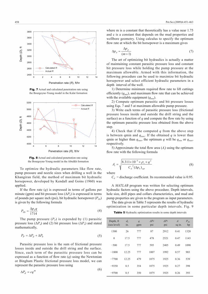
A MATLAB program was written to calculate coefficients with the genetic algorithm and eventually model the penetration rate of the Khangiran formations. Table 4 shows the computed constants of four formations of the Khangiran fi eld. Fig. 7 and Fig. 8 show the actual and calculated penetration rate using Bourgoyne-Young model in Kalat and Abtalkh formations, respectively. As obviously seen in these figures, the Bourgoyne-Young model estimates the penetration rate with reasonable accuracy.

4.5.2 Hydraulic optimizationMud and hydraulics are two of the most important factors

affecting the optimization of drilling operations. Without the optimum mud and hydraulics, the weight-rotational speed program cannot be fully implemented (Lummus, 1970).

As mentioned previously, many issues must be taken into account when optimizing drilling fl uids. Therefore, to simplify the optimization process, optimized drilling fl uid parameters achieved in comparative optimization process are applied.

Formation a1 a2 a3 a4 a5 a6 a7 a8

Khangiran 1.7 0.00002 0.0000008 0.000011 0.800 1 1 0.15

Kalat 1.30 0.000018 0.000002 0.00001 1.725 0.43 0.42 0.22

Abtalkh 1.22 0.000008 0.0000008 0.00001 0.863 0.68 0.58 0.15

Mozdouran 0.66 0.000008 0.0000008 0.00001 0.8 0.4 1.35 0.15

Table 4 Computed constants for four formations of the Khangiran fi eld

Pet.Sci.(2009)6:451-463

458

To optimize the hydraulic parameters like flow rate, pump pressure and nozzle sizes when drilling a well in the Khangiran field, the method of maximum bit hydraulic horsepower, developed by Kendall and Goins (1960) was applied.

If the flow rate (q) is expressed in terms of gallons per minute (gpm) and bit pressure loss (ΔPb) is expressed in terms of pounds per square inch (psi), bit hydraulic horsepower (PHb) is given by the following formula

(4)1714

qpP b

Hb

The pump pressure (PP) is expended by (1) parasitic pressure loss (ΔPd) and (2) bit pressure loss (ΔPb) and stated mathematically,

(5)bdP PPP

Parasitic pressure loss is the sum of frictional pressure losses inside and outside the drill string and the surface. Since, each term of the parasitic pressure loss can be expressed as a function of fl ow rate (q) using the Newtonian or Bingham Plastic frictional pressure loss model, we can represent the parasitic pressure loss using

(6)md cqP

where m is a constant that theoretically has a value near 1.75 and c is a constant that depends on the mud properties and wellbore geometry. Using calculus to specify the optimum fl ow rate at which the bit horsepower is a maximum gives

(7))1(m

pp p

d

The art of optimizing bit hydraulics is actually a matter of maintaining constant parasitic pressure loss and constant bit pressure loss while holding the pump pressure at the maximum allowable. Armed with this information, the following procedure can be used to maximize bit hydraulic horsepower and select efficient hydraulic parameters in a depth interval of the well.

1) Determine minimum required fl ow rate to lift cuttings effi ciently (qmin), and maximum fl ow rate that can be achieved with the available equipment (qmin).

2) Compute optimum parasitic and bit pressure losses using Eqs. 7 and 5 at maximum allowable pump pressure.

3) Write each terms of parasitic pressure loss (frictional pressure losses inside and outside the drill string and the surface) as a function of q and compute the fl ow rate by using the optimum parasitic pressure loss obtained from the above step.

4) Check that if the computed q from the above step is between qmin and qmax. If the obtained q is lower than qmin or higher than qmax, the optimum q will be qmin or qmax, respectively.

5) Approximate the total fl ow area (At) using the optimum fl ow rate with the following formula

(8)optbd

ct pC

qA

)(10311.82

25

whereCd = discharge coeffi cient. Its recommended value is 0.95.

A MATLAB program was written for selecting optimum hydraulic factors using the above procedure. Depth intervals, hole size, drill pipes and collars characteristics, and mud and pump properties are given to the program as input parameters.

The data given in Table 5 represents the results of hydraulic optimization in some particular depth intervals. Fig. 9

Fig. 7 Actual and calculated penetration rate usingthe Bourgoyne-Young model in the Kalat formation

0 2 4 6 8 10 12 142400

2600

2800

3000

3200

3400

3600

3800

Penetration rate (R), ft/hr

Dep

th (D

), ft

Calculated RActual R

Fig. 8 Actual and calculated penetration rate usingthe Bourgoyne-Young model in the Abtalkh formation

4 6 8 10 12 144000

4200

4400

4600

4800

5000

5200

Penetration rate (R), ft/hr

Dept

h (D

), ft

Calculated RActual R

Depth, ft(sea level)

db in.

q gpm

ΔPd

psiΔPb psi

A sq in.

PHb

hp

1300 26 777 87 2912 0.41 1320

0 17.5 777 478 2521 0.47 1143

−500 17.5 777 595 2405 0.49 1090

−1800 12.25 777 1007 1992 0.57 903

−7700 12.25 479 1075 1925 0.36 539

−9350 8.5 354 1075 1925 0.27 398

−9700 8.5 350 1075 1925 0.26 393

Table 5 Hydraulic optimization results in some depth intervals

Pet.Sci.(2009)6:451-463

459

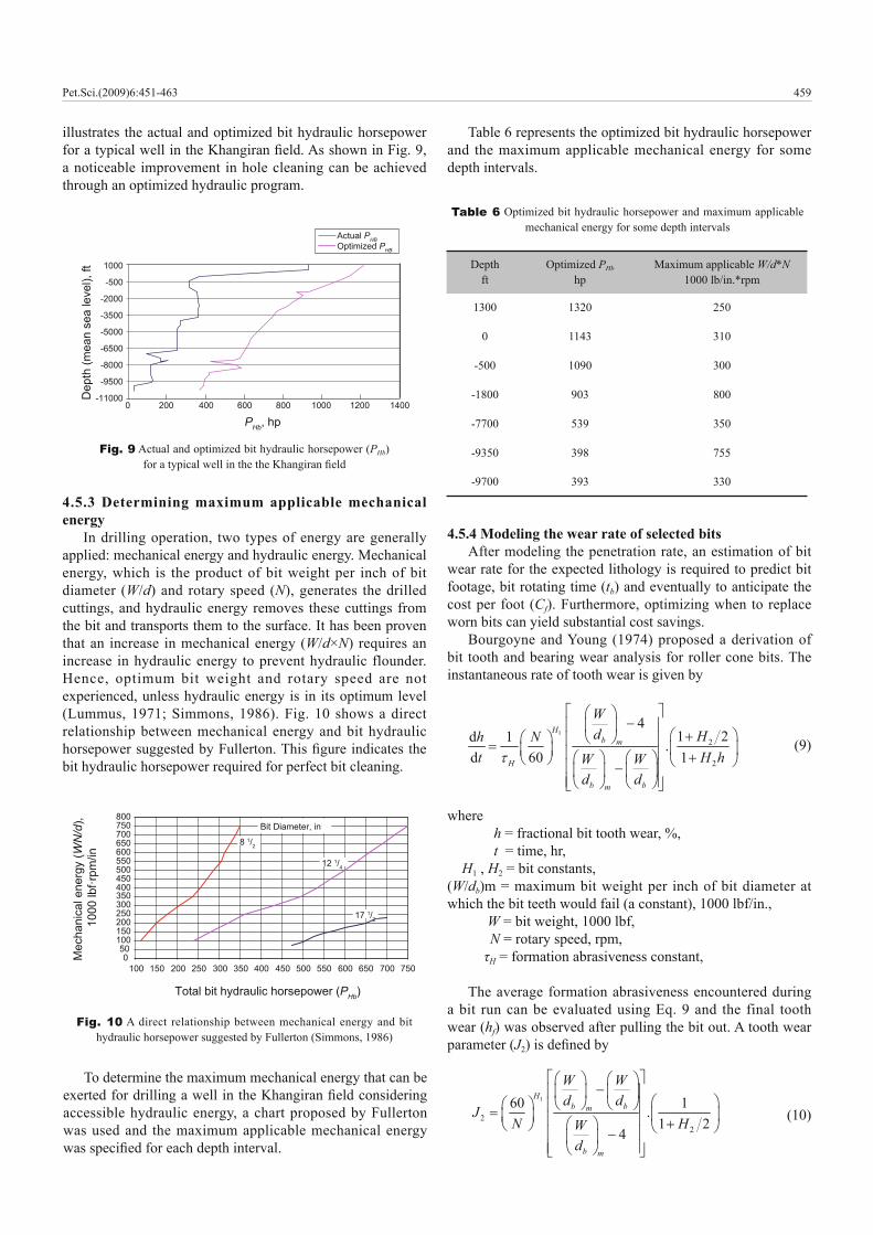
illustrates the actual and optimized bit hydraulic horsepower for a typical well in the Khangiran fi eld. As shown in Fig. 9, a noticeable improvement in hole cleaning can be achieved through an optimized hydraulic program.

Table 6 represents the optimized bit hydraulic horsepower and the maximum applicable mechanical energy for some depth intervals.

Fig. 9 Actual and optimized bit hydraulic horsepower (PHb) for a typical well in the the Khangiran fi eld

Actual PHBOptimized PHB

-11000

-9500

-8000

-6500

-5000

-3500

-2000

-500

1000

Dep

th (m

ean

sea

leve

l), ft

0 200 400 600 800 1000 1200 1400

PHb, hp

4.5.3 Determining maximum applicable mechanical energy

In drilling operation, two types of energy are generally applied: mechanical energy and hydraulic energy. Mechanical energy, which is the product of bit weight per inch of bit diameter (W/d) and rotary speed (N), generates the drilled cuttings, and hydraulic energy removes these cuttings from the bit and transports them to the surface. It has been proven that an increase in mechanical energy (W/d×N) requires an increase in hydraulic energy to prevent hydraulic flounder. Hence, optimum bit weight and rotary speed are not experienced, unless hydraulic energy is in its optimum level (Lummus, 1971; Simmons, 1986). Fig. 10 shows a direct relationship between mechanical energy and bit hydraulic horsepower suggested by Fullerton. This fi gure indicates the bit hydraulic horsepower required for perfect bit cleaning.

050

100150200250300350400450500550600650700750800

100 150 200 250 300 350 400 450 500 550 600 650 700 750

Total bit hydraulic horsepower (PHb)

Mec

hani

cal e

nerg

y (W

N/d

), 1

000

lbf·r

pm/in

Bit Diameter, in

8 1/2

12 1/4

17 1/2

Fig. 10 A direct relationship between mechanical energy and bit hydraulic horsepower suggested by Fullerton (Simmons, 1986)

To determine the maximum mechanical energy that can be exerted for drilling a well in the Khangiran fi eld considering accessible hydraulic energy, a chart proposed by Fullerton was used and the maximum applicable mechanical energy was specifi ed for each depth interval.

Depth ft

Optimized PHb hp

Maximum applicable W/d*N1000 lb/in.*rpm

1300 1320 250

0 1143 310

-500 1090 300

-1800 903 800

-7700 539 350

-9350 398 755

-9700 393 330

Table 6 Optimized bit hydraulic horsepower and maximum applicable mechanical energy for some depth intervals

4.5.4 Modeling the wear rate of selected bitsAfter modeling the penetration rate, an estimation of bit

wear rate for the expected lithology is required to predict bit footage, bit rotating time (tb) and eventually to anticipate the cost per foot (Cf). Furthermore, optimizing when to replace worn bits can yield substantial cost savings.

Bourgoyne and Young (1974) proposed a derivation of bit tooth and bearing wear analysis for roller cone bits. The instantaneous rate of tooth wear is given by

(9)1

2

2

41 2d 1 .

d 60 1

Hb m

H

b bm

Wd Hh N

t H hW Wd d

where h = fractional bit tooth wear, %, t = time, hr,

H1 , H2 = bit constants,(W/db)m = maximum bit weight per inch of bit diameter at which the bit teeth would fail (a constant), 1000 lbf/in.,

W = bit weight, 1000 lbf, N = rotary speed, rpm, τH = formation abrasiveness constant,

The average formation abrasiveness encountered during a bit run can be evaluated using Eq. 9 and the final tooth wear (hf) was observed after pulling the bit out. A tooth wear parameter (J2) is defi ned by

(10)1

22

60 1.1 2

4

Hb bm

b m

W Wd d

JN HW

d

Pet.Sci.(2009)6:451-463

460

Using calculus to solve for bit rotating time (tb) yields

(11)22 2( 2)b H f ft J h H h

Solving for the abrasiveness constant gives

(12)22 2( 2)

bH

f f

tJ h H h

A bearing wear formula frequently used to estimate bearing life is given by

(13)1 2d 1 ( ) ( )d 60 4

B B

B b

b N Wt d

where

b = fractional bearing life that has been consumed, %,B1, B2= bearing wear exponents,

db = bit diameter, in.,h = fractional bit tooth wear, %,τB = bearing constant,

If the bearing wear parameter is defi ned by

(14)1 23

460( ) ( )B BbdJN W

Solving Eq. 14 to fi nd tb gives

(15)3b B ft J b

where bf is the fi nal bearing wear observed after pulling the bit out. Solving Eq. 13 for the bearing constant gives

(16)3

bB

f

tJ b

To compute the average abrasiveness constant (τH) for each formations of Khangiran field and bearing constant (τB) for each selected bit using Eqs. 12 and 16, a MATLAB program was written. Required drilling records at final bit dullness are the input parameters of this program.

It is worth noting that Eqs. 9 and 13 were developed for use in modelling the wear rate of roller cone bits. Unfortunately, widely used numerical models for estimating the wear rate of PDC bits have not yet been developed. Hence, to apply the wear rate models in depth intervals in which PDC bits were selected previously, the best examined roller cone bits must be substituted.

Table 7 shows the computed formation abrasiveness constants of the Khangiran field. Table 8 presents the computed bearing constants of some chosen bits in optimal wells. As seen in Table 7, Shourijeh (a reservoir) and Abderaz are the highest and lowest abrasive formations in the Khangiran fi eld, respectively.4.5.5 Selecting optimum bit weight and rotary speed

As discussed in the above sections, bit weight and rotational speed of the drill string have a major effect on both the penetration rate and the bit life. In determining the best bit weight and rotary speed for a given formation, the following

items must be taken into consideration: (1) the effect of the selected operating conditions on the cost per foot for the bit run, (2) the effect of the selected bit weight/rotary speed on crooked hole problems, (3) the maximum mechanical energy (W/d×N) that can be applied based on the maximum achievable bit hydraulic horsepower, and (4) equipment limitations on the available bit weight/rotary speed.

In many instances, a wide range of bit weights and rotary speed can be selected without creating crooked hole problems and besides, such kind of problems can be reduced noticeably with proper design of the bottom hole assembly (BHA). Under these conditions, selecting the best bit weight/rotary speed that will result in minimum cost per foot is limited to maximum applicable mechanical energy (W/d×N) and bit operating ranges recommended by manufacturing companies.

Several methods are available for computing both the best variable bit weight/rotary speed schedule and the best constant bit weight/rotary speed schedule to achieve minimum drilling cost per foot. Some authors have reported that there is a slightly difference between cost per foot results

Formation Abrasiveness constant (τH)

Khangiran 378

Chehelkaman 392

Kalat 137

Neyzar 141

Abtalkh 373

Abderaz 479

Aytamir 441

Sanganeh 390

Sarcheshmeh 317

Shourijeh 64

Mozdouran 79

Table 7 Computed formations abrasiveness constants of Khangiran fi eld

Bit type IADC code Bearing constant (τB)

Y13 131 28

S4T 133 38

SDJH 135 71

M44L 234 67

S84F 517 150

Table 8 Computed bearing constants of some chosen bits in optimal well

Pet.Sci.(2009)6:451-463

461

of variable and constant bit weight/rotary speed schedule for the cases studied (Bourgoyne et al, 2003).

One straightforward technique used for determining the best combination of constant bit weight/rotary speed is to generate a cost per foot table, using the assumed bit weights and rotary speeds considering the operational constraints, but in advance, the following mathematical constrained optimization problem must be solved:

(17)Min ( , )fC f W d N

Constraints: 1 1

2 2

/

lb W d ublb N ubW d N M

where W/d = bit weight per inch of bit diameter, lb1 = lower bound of bit weight per inch of bit diameter, lb2 = lower bound of rotary speed, ub1 = upper bound of bit weight per inch of bit diameter, ub2 = upper bound of rotary speed, M = maximum applicable mechanical energy (W/d×N), N = rotary speed.

In this problem, the upper and lower bounds of bit weight and rotary speed are provided by bit operating ranges, which are recommended by manufacturing companies.

In order to compute the cost per foot with the assumed bit weight and rotary speed, Bourgoyne et al (2003) suggested a formula to predict the footage that would be drilled (ΔD) in a given time interval. If a composite drilling variable (J1) is defi ned by

(18) 86543211 fffffffJ

Eq. 3a can be expressed by

(19) 71 7 1

dd

a hDR J f J et

Using bit wear equations to solve the bit footage (ΔD) in terms of the fi nal tooth wear (hf) yields

27

77

72

7

7

21

1(1a

ehaeHaeJJD

fhaf

fhafha

H

(20)

When Bourgoyne-Young penetration rate and bit wear models are applied, the following procedure could be used to predict the cost per foot associated with complete bit wear for each bit weight/rotary speed set (Bourgoyne et al, 2003).

1) Assume a bit weight and rotary speed, considering the operational constraints.

2) Compute the times required to wear out the bit teeth using Eq. 11.

3) Compute the times required to wear out the bearings using Eq. 15.

4) Using the smaller time of the two computed times, estimate the footage (ΔD) that would be drilled using Eq. 20.

5) Compute the cost per foot using Eq. 1.To apply the above procedure for selection of optimum bit

weight/rotary speed in various depths of the Khangiran fi eld, a MATLAB program was written. This program is equipped with a constrained optimization algorithm called trust region (Coleman, 1996). In each iteration step, a set of bit weight/rotary speed considering the operational bonds is assumed and then the cost per foot is computed using the described procedure. Iterations are continued until the cost per foot is minimized. Required data for simultaneous modeling of penetration rate and bit wear rate are given to the program as input parameters. Note that, input parameters have been optimized in the previous steps and, after the selection of appropriate bit weight and rotational speed for each depth of the Khangiran fi eld, the mathematical optimization process is completed and the secondary optimal well is achieved.

Fig. 11 shows a three-dimensional view of cost per foot surface versus bit weight and rotary speed for the depth of 1800 ft. As can be seen, the minimum cost per foot in this depth is obtained when W=55000 lb and N=140 rpm.

Fig. 11 A 3-D view of cost per foot surface versus bit weight and rotary speed for the depth 1800 ft

6080

100120

140160

202530354045505560 W, 1000 lbN, rpm

Cf,

$/ft

25

31

28

43

40

37

34

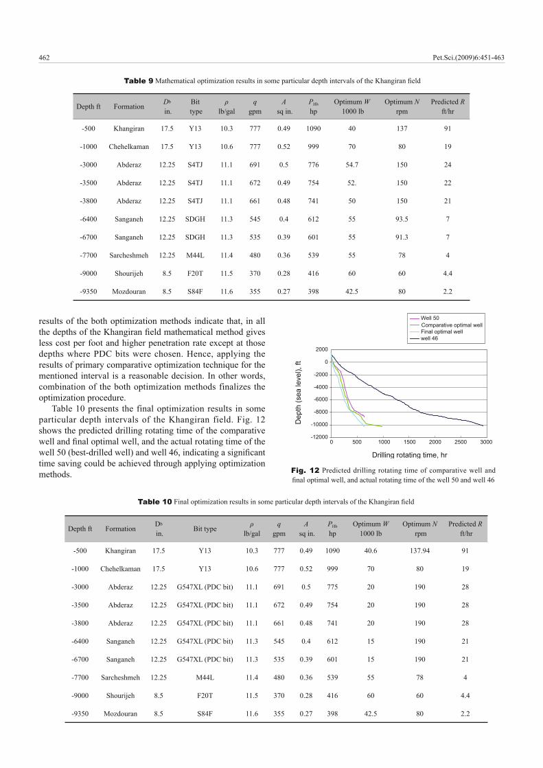
Table 9 summarizes the mathematical optimization results in some particular depth intervals of Khangiran fi eld.

4.6 Combination of comparative and mathematical optimization techniques

In the fi nal step of the optimization procedure, combining the results of comparative and mathematical optimization methods in some depth intervals seems to be essential.

As discussed above, when the comparative technique was applied in the Khangiran fi eld, PDC bits were selected in the interval of -1400 ft to -7400 ft since they exhibited very high performance in one drilled well. However, because popular numerical models for estimating the wear rate of PDC bits have not yet been developed, to apply mathematical techniques in these intervals, we were forced to model the wear rate of the best-examined roller cone bits, instead. The

Pet.Sci.(2009)6:451-463

462

results of the both optimization methods indicate that, in all the depths of the Khangiran fi eld mathematical method gives less cost per foot and higher penetration rate except at those depths where PDC bits were chosen. Hence, applying the results of primary comparative optimization technique for the mentioned interval is a reasonable decision. In other words, combination of the both optimization methods finalizes the optimization procedure.

Table 10 presents the final optimization results in some particular depth intervals of the Khangiran field. Fig. 12 shows the predicted drilling rotating time of the comparative well and fi nal optimal well, and the actual rotating time of the well 50 (best-drilled well) and well 46, indicating a signifi cant time saving could be achieved through applying optimization methods.

Depth ft Formation Db

in.Bit

typeρ

lb/galq

gpmA

sq in.PHb

hpOptimum W

1000 lbOptimum N

rpmPredicted R

ft/hr

-500 Khangiran 17.5 Y13 10.3 777 0.49 1090 40 137 91

-1000 Chehelkaman 17.5 Y13 10.6 777 0.52 999 70 80 19

-3000 Abderaz 12.25 S4TJ 11.1 691 0.5 776 54.7 150 24

-3500 Abderaz 12.25 S4TJ 11.1 672 0.49 754 52. 150 22

-3800 Abderaz 12.25 S4TJ 11.1 661 0.48 741 50 150 21

-6400 Sanganeh 12.25 SDGH 11.3 545 0.4 612 55 93.5 7

-6700 Sanganeh 12.25 SDGH 11.3 535 0.39 601 55 91.3 7

-7700 Sarcheshmeh 12.25 M44L 11.4 480 0.36 539 55 78 4

-9000 Shourijeh 8.5 F20T 11.5 370 0.28 416 60 60 4.4

-9350 Mozdouran 8.5 S84F 11.6 355 0.27 398 42.5 80 2.2

Table 9 Mathematical optimization results in some particular depth intervals of the Khangiran fi eld

Fig. 12 Predicted drilling rotating time of comparative well and fi nal optimal well, and actual rotating time of the well 50 and well 46

-12000

-10000

-8000

-6000

-4000

-2000

0

2000

0 500 1000 1500 2000 2500 3000

Drilling rotating time, hr

Dep

th (s

ea le

vel),

ft

Well 50Comparative optimal wellFinal optimal wellwell 46

Depth ft Formation Db

in. Bit type ρlb/gal

qgpm

A sq in.

PHb

hpOptimum W

1000 lbOptimum N

rpmPredicted R

ft/hr

-500 Khangiran 17.5 Y13 10.3 777 0.49 1090 40.6 137.94 91

-1000 Chehelkaman 17.5 Y13 10.6 777 0.52 999 70 80 19

-3000 Abderaz 12.25 G547XL (PDC bit) 11.1 691 0.5 775 20 190 28

-3500 Abderaz 12.25 G547XL (PDC bit) 11.1 672 0.49 754 20 190 28

-3800 Abderaz 12.25 G547XL (PDC bit) 11.1 661 0.48 741 20 190 28

-6400 Sanganeh 12.25 G547XL (PDC bit) 11.3 545 0.4 612 15 190 21

-6700 Sanganeh 12.25 G547XL (PDC bit) 11.3 535 0.39 601 15 190 21

-7700 Sarcheshmeh 12.25 M44L 11.4 480 0.36 539 55 78 4

-9000 Shourijeh 8.5 F20T 11.5 370 0.28 416 60 60 4.4

-9350 Mozdouran 8.5 S84F 11.6 355 0.27 398 42.5 80 2.2

Table 10 Final optimization results in some particular depth intervals of the Khangiran fi eld

Pet.Sci.(2009)6:451-463

463

5 Conclusion Systematic combination of theory and application in this

study for optimizing drilling parameters of Iranian Khangiran gas fi eld provides a dramatic saving of time and money for further drilling operation in this fi eld. Whenever the records of more drilled wells are analyzed in the optimization process, the accuracy of the drilling optimization would be improved.

Although, optimizing drilling variables for the phase of bit rotating time is the most important matter when a well is being drilled, other optimization techniques should also be employed to reduce the drilling problems and achieve a short non-rotating time of the drill string and as a result, lower the drilling time and cost. This issue needs considerable work in the future for the fi eld studied.

AcknowledgementsThe authors would like to thank the drilling engineering

manager and staffs of Iranian Central Oil Fields Company (I.C.O.F.C) for their contribution and cooperation in this research.

Conversion Factors ft × 3.048 E − 01 = m hp × 7.46043 E − 01 = kW cp × 1.0 E − 03 = Pa.s lbf × 4.44822 E + 00 = Nlbm × 4.535 92 E − 01 = kg ft3 × 2.831 68 E − 02 = m3

ReferencesBah ari A and Baradaran Seyed A. Trust-region approach to fi nd constants

of Bourgoyne and Young penetration rate model in Khangiran Iranian Gas Field. Paper SPE 107520 accepted for presentation in 2007 SPE Latin American and Caribbean Petroleum Engineering

Conference, Buenos Aires, Argentina, 15-18 April, 2007Bah ari A and Baradaran Seyed A. Drilling cost optimization in Iranian

Khangiran Gas Field. Paper SPE 108246 accepted for presentation in 2007 International Oil Conference and Exhibition in Mexico, Veracruz, Mexico, 27-30 June, 2007

Bah ari M H, Bahari A, Nejati Moharrami F and Naghibi Sistani M B. Determining Bourgoyne and Young model coeffi cients using genetic algorithm to predict drilling rate. Journal of Applied Sciences. 2008. 8 (17): 3050-3054

Bil gesu H I, Tetrick L T, Altmis U, Mohaghegh S and Ameri S. A new approach for the prediction of rate of penetration values. Paper presented at SPE Eastern Regional Meeting, Lexington, USA, 1997

Bou rgoyne A T, Millheim K K, Chenevert M E and Young F S. Applied Drilling Engineering. Richardson, TX., SPE textbook series, 2003. Vol. 2: 237-240

Bou rgoyne A T and Young F S. A multiple regression approach to optimal drilling and abnormal pressure detection. SPE 4238, SPEJ; Trans. 1974. 257: 371-384

Col eman T F and Li Y. An Interior, Trust region approach for nonlinear minimization subject to bounds. SIAM J. Opt. 1996. 6: 418

Kai ser M J. A Survey of drilling cost and complexity estimation models. Int. J. Pet. Sci. Technol. 2007. 1: 1-22

Ken dall H A and Goins W C. Design and operation of jet-bit programs for maximum hydraulic horsepower, impact force or jet velocity. Petroleum Transactions, AIME. 1960. 219: 238-250

Lum mus J L. Drilling Optimization. AIME/SPE 2744, JPT. 1970. 1379-1388

Lum mus J L. Acquisition and analysis of data for optimized drilling. AIME/SPE 3716, JPT. 1971. 1285-1293

Njo buenwu D O and Wobo C A. Effect of drilled solids on drilling rate and performance. Journal of Petroleum Science and Engineering. 2007. 55 (3-4): 271-276

Rab ia H. Specifi c energy as a criterion for bit selection. JPT. July, 1985. 1225-1229

Sim mons E L. A Technique for accurate bit programming and drilling performance optimization. Paper IADC/SPE 14784 presented at the 1986 IADC/SPE Drilling Conference, Dallas, TX, Feb. 1986. 10–12

(Edited by Zhu Xiuqin)

Pet.Sci.(2009)6:451-463