Embed Size (px)
Citation preview
DrakeDRAKE UNIVERSITY
Fin 288
Interest Rates and price determination
Fin 288Futures Options and Swaps
DrakeDrake University
Fin 288
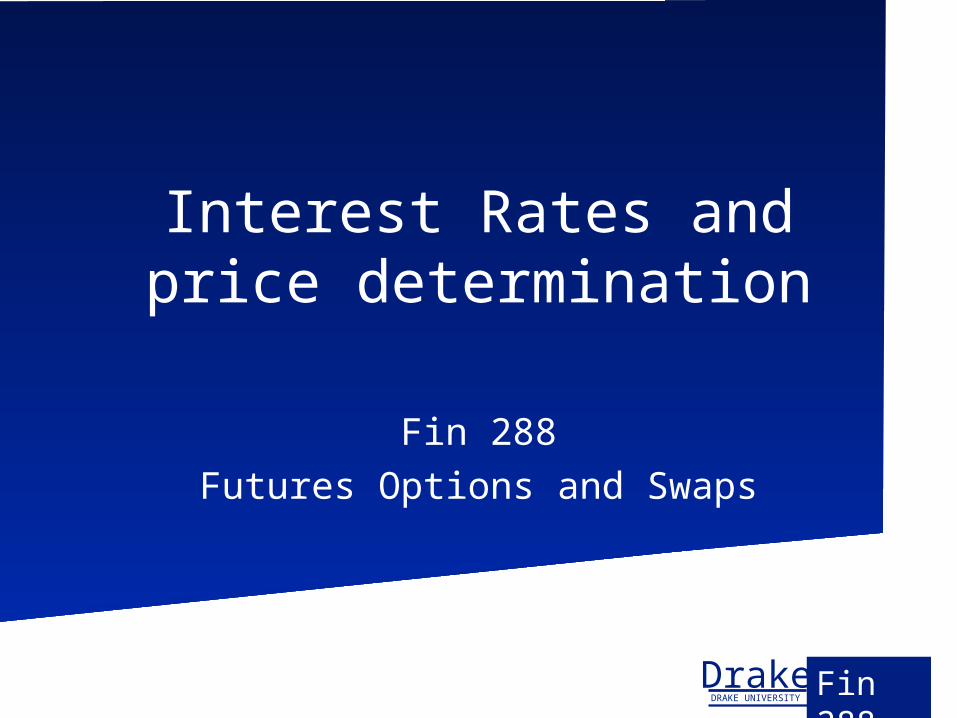
PV and FV in continuous time
e = 2.71828 y = lnx x = ey
FV = PV (1+k)n for yearly compoundingFV = PV(1+k/m)nm for m compounding
periods per yearAs m increases this becomesFV = PVern =PVert let t =n rearranging for PV PV = FVe-rt
DrakeDrake University
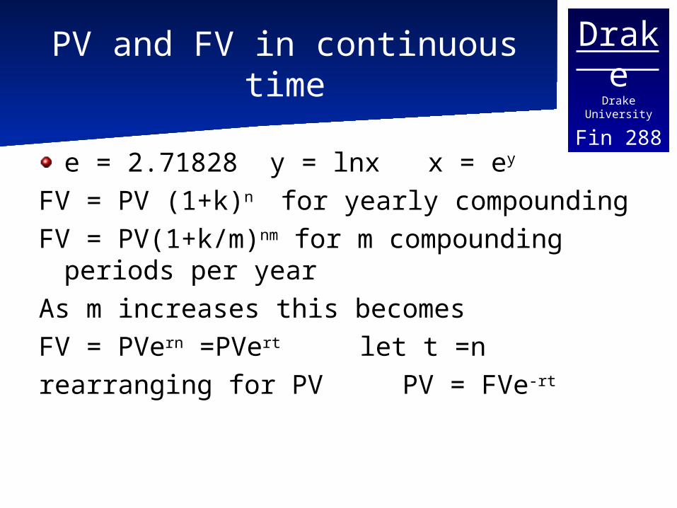
Fin 288Compounding periods
The PV of $100 assuming 8% per year a various compounding periods for 5 years.
# of periods per year
PV
2 44.63
4 45.29
12 45.05
52 44.96
continuous 44.93
DrakeDrake University
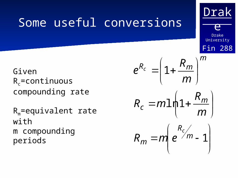
Fin 288Some useful conversions
1
1ln
1
mR
m
mc
mmR
c
c
emR
m
RmR
m
ReGiven
Rc=continuous compounding rate
Rm=equivalent rate with m compounding periods
DrakeDrake University
Fin 288A General Valuation Model
The basic components of valuing any asset are:
An estimate of the future cash flow stream from owning the assetThe required rate of return for each period based upon the riskiness of the asset
The value is then found by discounting each cash flow by its respective discount rate and then summing the PV’s (Basically the PV of an Uneven Cash Flow Stream)
DrakeDrake University
Fin 288
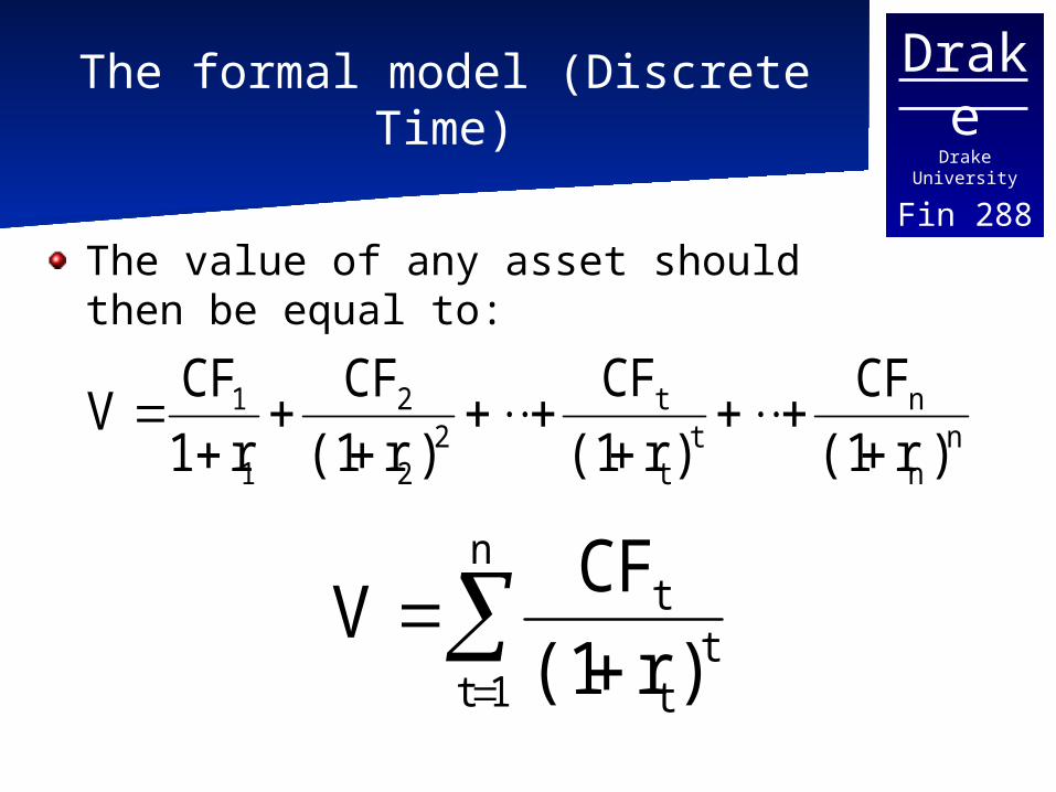
The formal model (Discrete Time)
The value of any asset should then be equal to:
nn
nt
t
t2
2
2
1
1
)r(1
CF
)r(1
CF
)r(1
CF
r1
CFV
n
1tt
t
t
)r(1
CFV
DrakeDrake University
Fin 288
Components of the General Model
Cash Flow at time t (CFt): the expected future cash flow that the owner of the asset expects to receive at time t.
The future cash flow may not be known with certainty.
The Discount Rate: The return that investors in the market are requiring for owning the asset.
The discount rate should reflect the risks faced by the investor. What risks are faced???
DrakeDrake University
Fin 288The Discount Rate
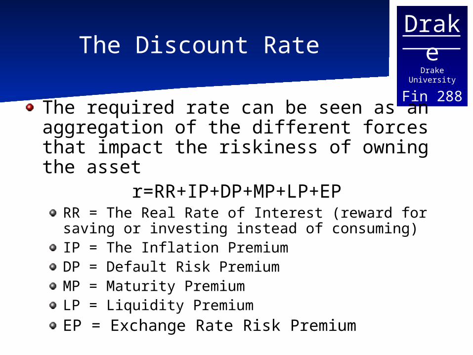
The required rate can be seen as an aggregation of the different forces that impact the riskiness of owning the asset
r=RR+IP+DP+MP+LP+EPRR = The Real Rate of Interest (reward for saving or investing instead of consuming)IP = The Inflation PremiumDP = Default Risk PremiumMP = Maturity PremiumLP = Liquidity PremiumEP = Exchange Rate Risk Premium
DrakeDrake University
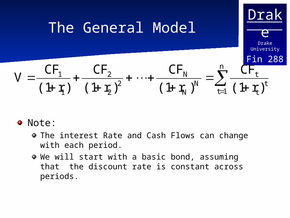
Fin 288The General Model
Note:The interest Rate and Cash Flows can change with each period.We will start with a basic bond, assuming that the discount rate is constant across periods.
n
1tt
t
tN
N
N2
2
2
1
1
)r(1
CF
)r(1
CF
)r(1
CF
)r(1
CFV
DrakeDrake University
Fin 288
Applying the general valuation formula to a bond
What component of a bond represents the future cash flows?
Coupon Payment: The amount the holder of the bond receives in interest at the end of each specified period.The Par Value: The amount that will be repaid to the purchaser at the end of the debt agreement.
DrakeDrake University
Fin 288Basic Bond Mathematics
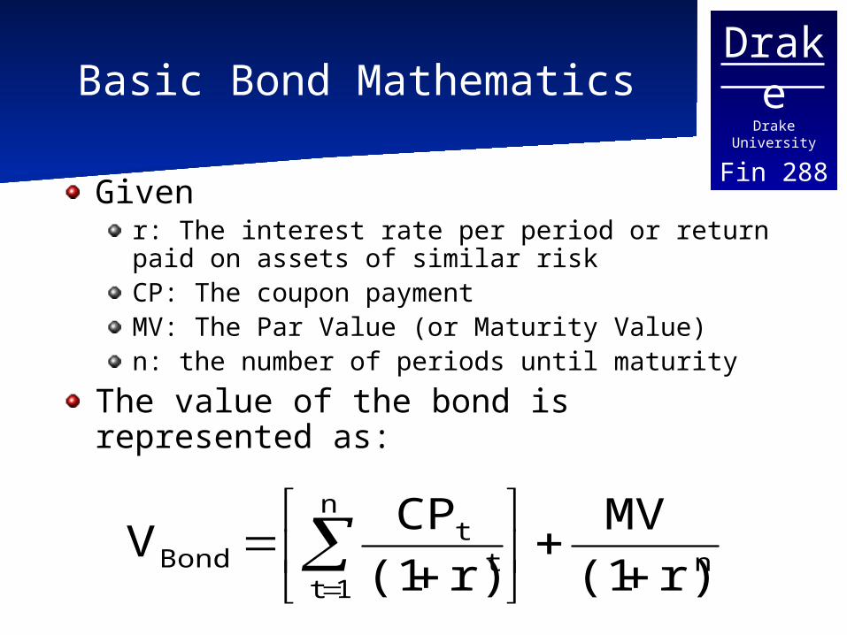
Givenr: The interest rate per period or return paid on assets of similar riskCP: The coupon paymentMV: The Par Value (or Maturity Value)n: the number of periods until maturity
The value of the bond is represented as:
n
n
1tt
tBond r)(1
MV
r)(1
CPV
DrakeDrake University
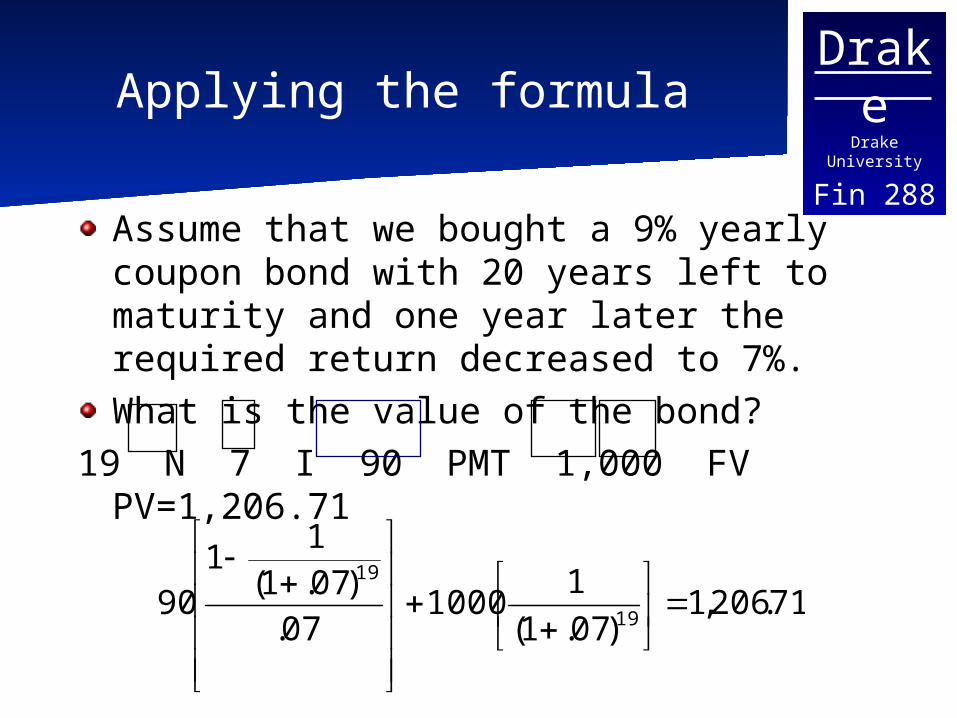
Fin 288Applying the formula
Assume that we bought a 9% yearly coupon bond with 20 years left to maturity and one year later the required return decreased to 7%.What is the value of the bond?
19 N 7 I 90 PMT 1,000 FV PV=1,206.71
71.206,1)07.1(
11000
07.)07.1(
11
9019
19
DrakeDrake University
Fin 288Why 1,206.71?
New bonds of similar risk are only paying a 7% return. This implies a coupon rate of 7% and a coupon payment of $70.The old bond has a coupon payment of $90, everyone will want to buy the old bond, (the increased demand increases the price)Why does it stop at $1,206.71?
If you bought the bond for $1,206.71 and received $90 coupon payments for the next 19 years you receive a 7% return.

DrakeDrake University
Fin 288Quick Facts for Review
If the level of interest rates in the economy increases the bond price decreases and vice versa.
If r>Coupon rate the price of the bond is below the par value - it sells at a discount.
If r<Coupon rate the price of the bond is above the par value - it sells at a premium.
Keeping everything constant the value of the bond will move toward par value as it gets closer to maturity.
DrakeDrake University
Fin 288
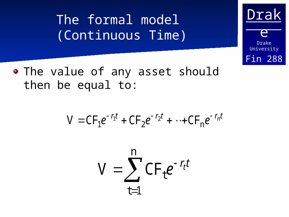
The formal model (Continuous Time)
The value of any asset should then be equal to:
trtrtr neee n21 CFCFCFV 21
n
1ttCFV trte
DrakeDrake University
Fin 288
A Package of Zero Coupon Bonds
You can think of a bond as a package of zero coupon bonds. Each payment received represents a zero coupon bond.Since yields differ with maturity, this implies that it does not make sense to use only one rate (the YTM) to value the bond.The value of the bond should be the same regardless of which way it is valued.
DrakeDrake University
Fin 288Stripped Coupons
If the value of the individual coupons is different from the entire bond it would be possible to buy the bond and sell the coupons as a security making a risk free profit.To value the stripped coupons each would be valued at a rate that matches its maturity, the rate should also represent a zero coupon bond.We can use the information in the market to create a zero coupon yield curve.
DrakeDrake University
Fin 288Zero Coupon (spot) Rates
The “n year spot interest rate” is the rate that would be earned today on an investment lasting n yearsAssumes that no interest or coupon payments are made. The Forward Rate will be the rate between two points in time in the future implied by the zero coupon yield curve
DrakeDrake University
Fin 288Spot Rate Yield Curve
The spot rate yield curve will be the value of the pot rate at different maturities. Often this is calculated for treasury securities – based on the assumption that treasuries are “risk free”
DrakeDrake University
Fin 288
Theoretical Spot Rate Curves
Two main issues1. Given a series of Treasury securities, how do
you construct the curve?a. Linear Extrapolationb. Bootstrappingc. Other
2. What Treasuries should be used to construct it?a. On the run Treasuriesb. On the run Treasuries and selected off the
run Treasuriesc. All Treasury Coupon Securities and Billsd. Treasury Coupon Strips
DrakeDrake University
Fin 288Observed Yields
For on-the-run treasury securities you can observe the current yield. For the coupon bearing bonds the yield used reflects the yield that would make it trade at par. The resulting on the run curve is the par coupon curve.However, you may have missing maturities for the on the run issues. Then you will need to estimate the missing maturities.
DrakeDrake University
Fin 288Example
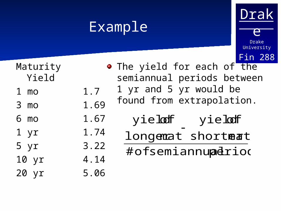
MaturityYield
1 mo 1.73 mo 1.696 mo 1.671 yr 1.745 yr 3.2210 yr 4.1420 yr 5.06
The yield for each of the semiannual periods between 1 yr and 5 yr would be found from extrapolation.
periods semiannual of #
matshorter
of yield
matlonger
of yield
DrakeDrake University
Fin 288
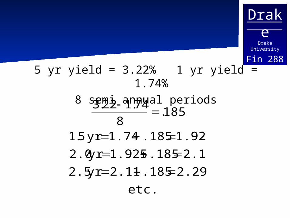
5 yr yield = 3.22% 1 yr yield = 1.74%8 semi annual periods
etc.
2.295.1852.11 yr 2.5
2.11 .1851.925 yr 2.0
1.925.185 1.74 yr 5.1
185.8
74.122.3
DrakeDrake University
Fin 288Bootstrapping
To avoid the missing maturities it is possible to estimate the zero spot rate from the current yields, and prices using bootstrapping. Bootstrapping successively calculates the next zero coupon from those already calculated.
DrakeDrake University
Fin 288
Treasury Bills vs. Notes and Bonds
Treasury bills are issued for maturities of one year or less. They are pure discount instruments (there is no coupon payment).Everything over two years is issued as a coupon bond.

DrakeDrake University
Fin 288Bootstrapping example
Assume we have the following on the run treasury bills and bonds:Assume that all coupon bearing bonds (greater than 1 year) are selling at par (constructing a par value yield curve)Maturity YTM Maturity YTM0.5 4% 2.5 5.0%1.0 4.2% 3.0 5.2%1.5 4.45% 3.5 5.4%2.0 4.75% 4.0 5.55%
DrakeDrake University
Fin 288Bootstrapping continued
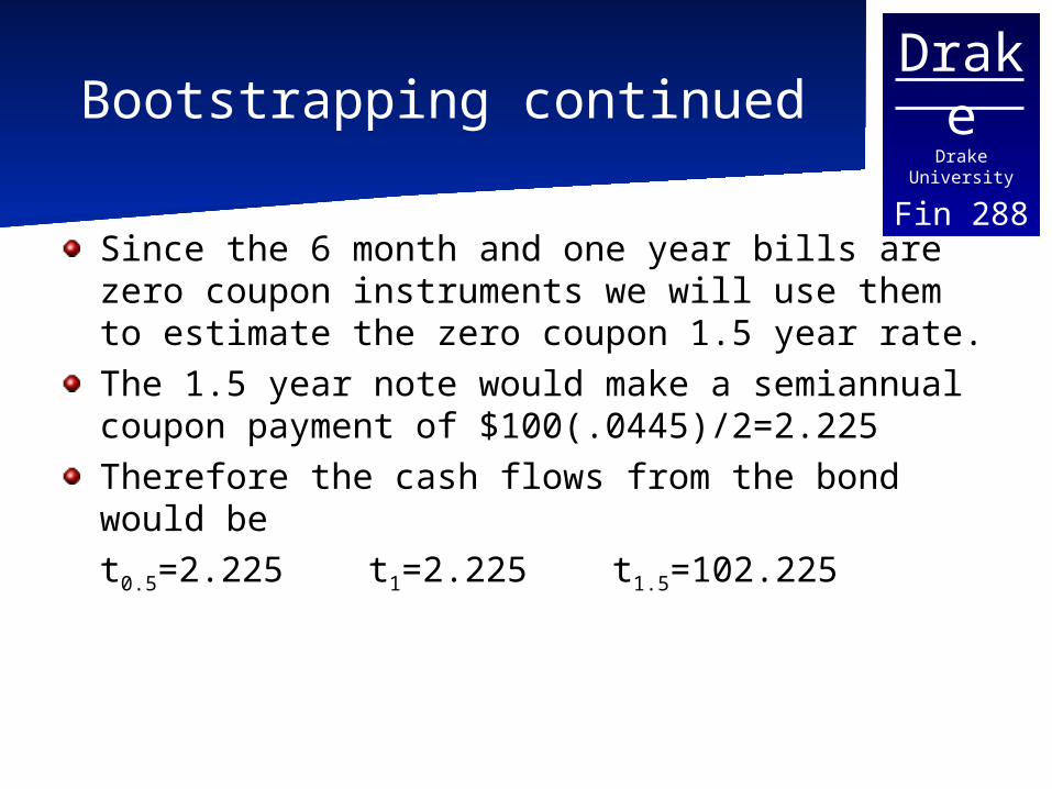
Since the 6 month and one year bills are zero coupon instruments we will use them to estimate the zero coupon 1.5 year rate.The 1.5 year note would make a semiannual coupon payment of $100(.0445)/2=2.225Therefore the cash flows from the bond would bet0.5=2.225 t1=2.225 t1.5=102.225
DrakeDrake University
Fin 288Bootstrapping continued
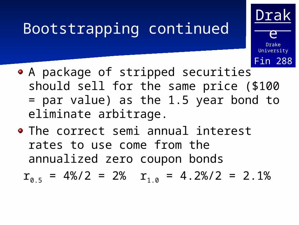
A package of stripped securities should sell for the same price ($100 = par value) as the 1.5 year bond to eliminate arbitrage.The correct semi annual interest rates to use come from the annualized zero coupon bonds
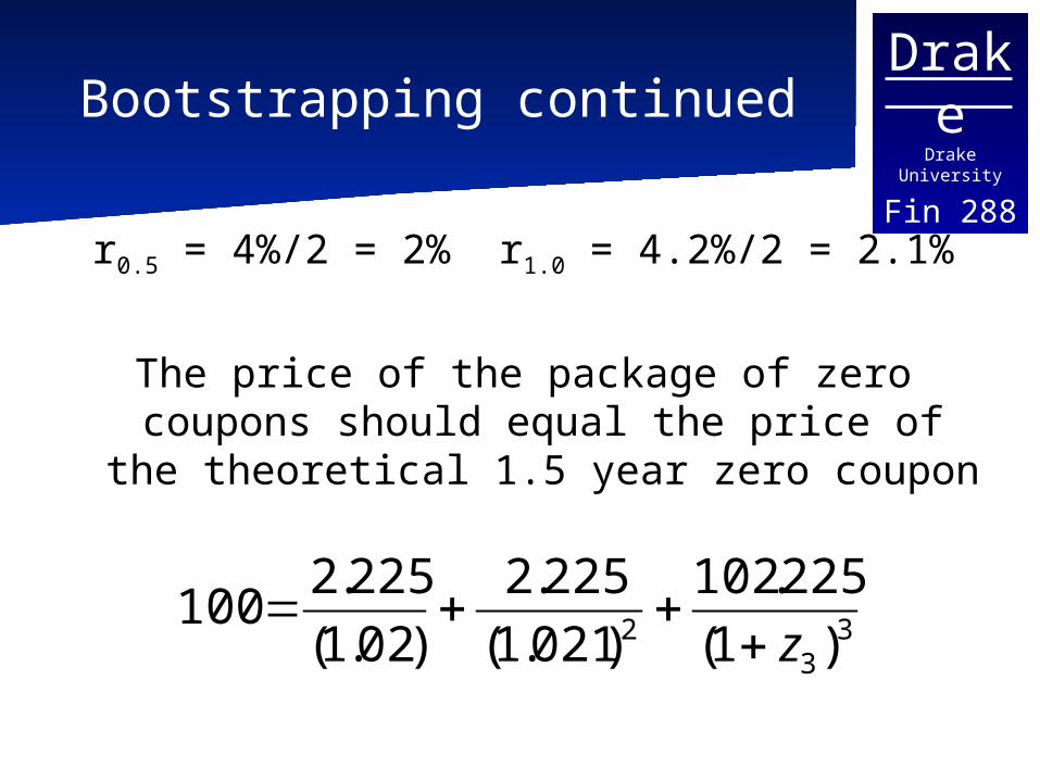
r0.5 = 4%/2 = 2% r1.0 = 4.2%/2 = 2.1%
DrakeDrake University
Fin 288Bootstrapping continued
r0.5 = 4%/2 = 2% r1.0 = 4.2%/2 = 2.1%
The price of the package of zero coupons should equal the price of the theoretical
1.5 year zero coupon
3
32 )1(
225.102
)021.1(
225.2
)02.1(
225.2100
z
DrakeDrake University
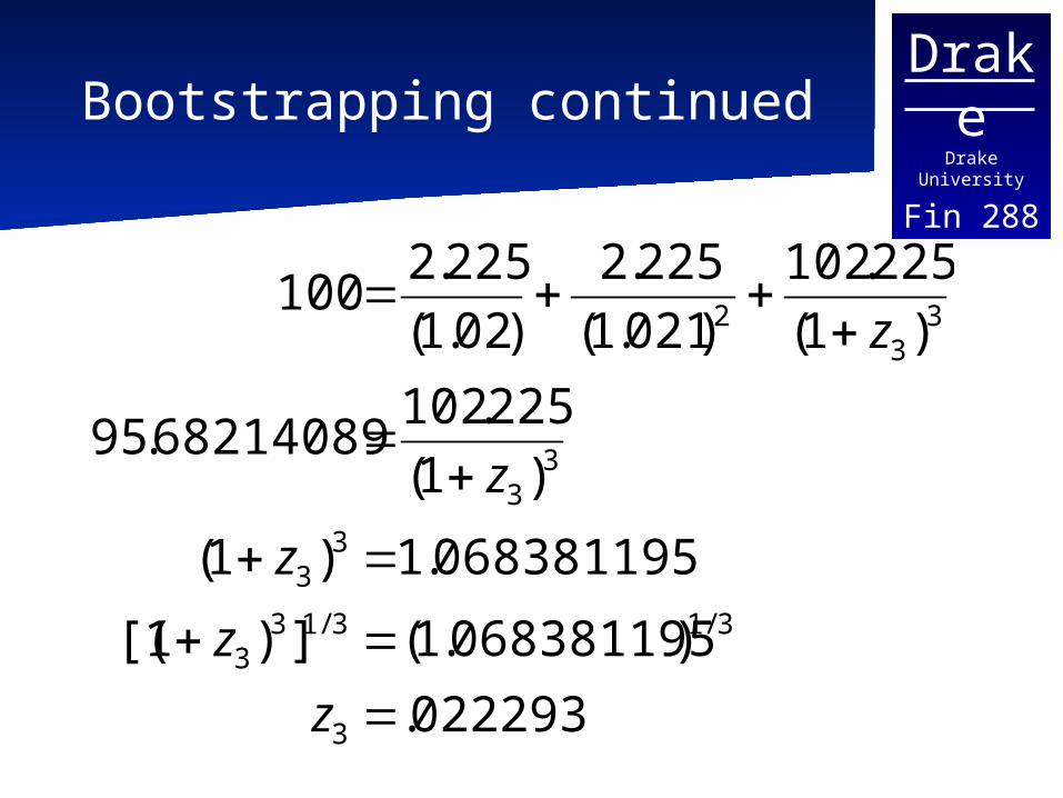
Fin 288Bootstrapping continued
022293.
)068381195.1(])1[(
068381195.1)1(
)1(
225.10268214089.95
)1(
225.102
)021.1(
225.2
)02.1(
225.2100
3
3/13/133
33
33
33
2
z
z
z
z
z
DrakeDrake University
Fin 288Bootstrapping continued
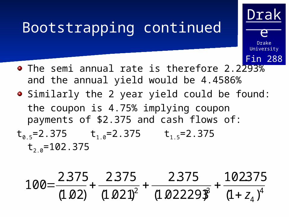
The semi annual rate is therefore 2.2293% and the annual yield would be 4.4586%Similarly the 2 year yield could be found:the coupon is 4.75% implying coupon payments of $2.375 and cash flows of:
t0.5=2.375 t1.0=2.375 t1.5=2.375 t2.0=102.375
44
32 )1(
375.102
)022293.1(
375.2
)021.1(
375.2
)02.1(
375.2100
z
DrakeDrake University
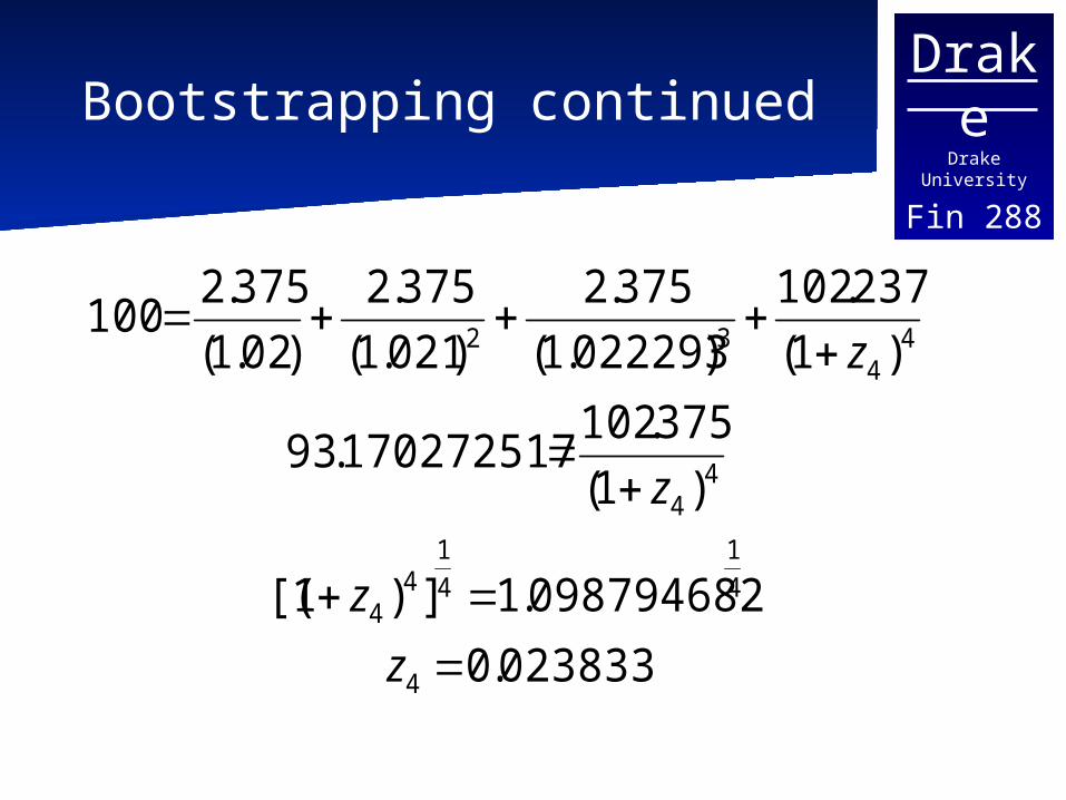
Fin 288Bootstrapping continued
023833.0
098794682.1])1[(
)1(
375.102170272517.93
)1(
237.102
)022293.1(
375.2
)021.1(
375.2
)02.1(
375.2100
4
4
1
4
14
4
44
44
32
z
z
z
z
DrakeDrake University
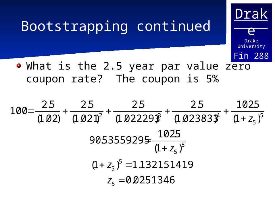
Fin 288Bootstrapping continued
What is the 2.5 year par value zero coupon rate? The coupon is 5%
0251346.0
132151419.1)1(
)1(
5.10253559295.90
)1(
5.102
)023833.1(
5.2
)022293.1(
5.2
)021.1(
5.2
)02.1(
5.2100
5
55
55
55
432
z
z
z
z
DrakeDrake University
Fin 288
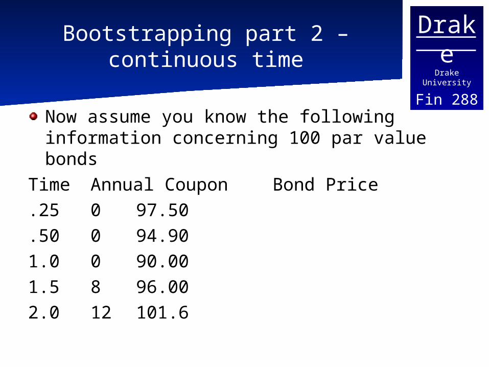
Bootstrapping part 2 – continuous time
Now assume you know the following information concerning 100 par value bonds
Time Annual CouponBond Price.25 0 97.50.50 0 94.901.0 0 90.001.5 8 96.002.0 12 101.6
DrakeDrake University
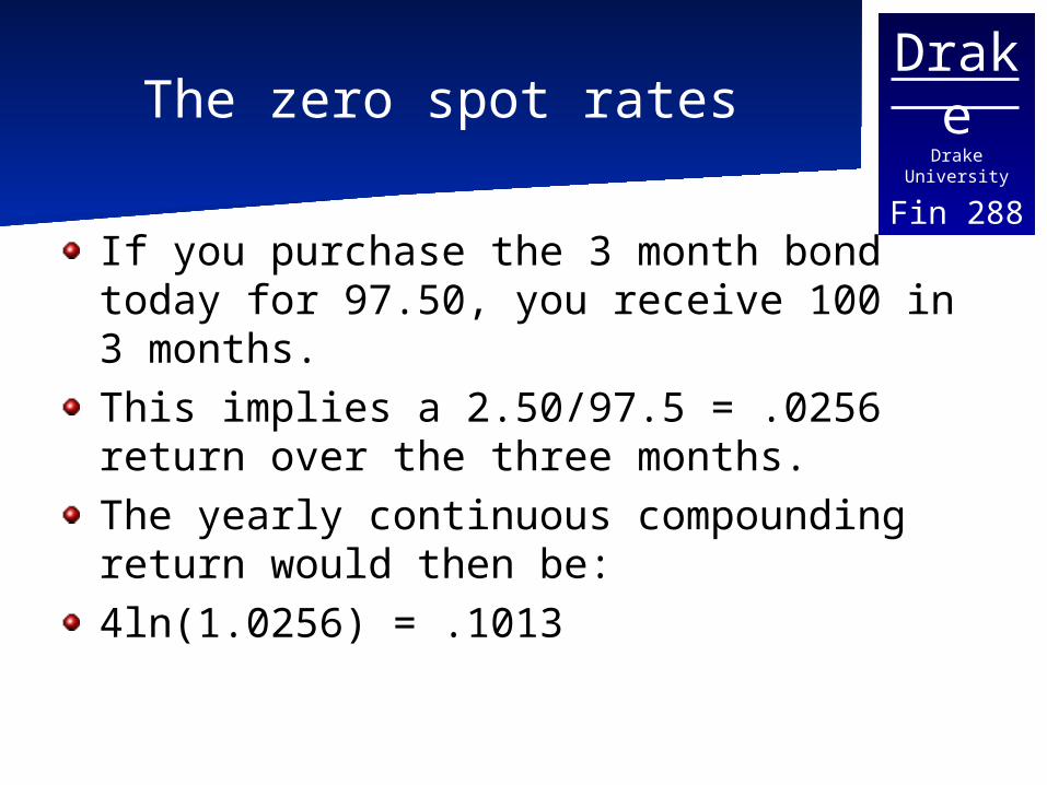
Fin 288The zero spot rates
If you purchase the 3 month bond today for 97.50, you receive 100 in 3 months.This implies a 2.50/97.5 = .0256 return over the three months. The yearly continuous compounding return would then be:4ln(1.0256) = .1013
DrakeDrake University
Fin 288Zero Coupon Rates
Similarly the 6 month rate would be .1047 and the one year rate would be .1054
DrakeDrake University
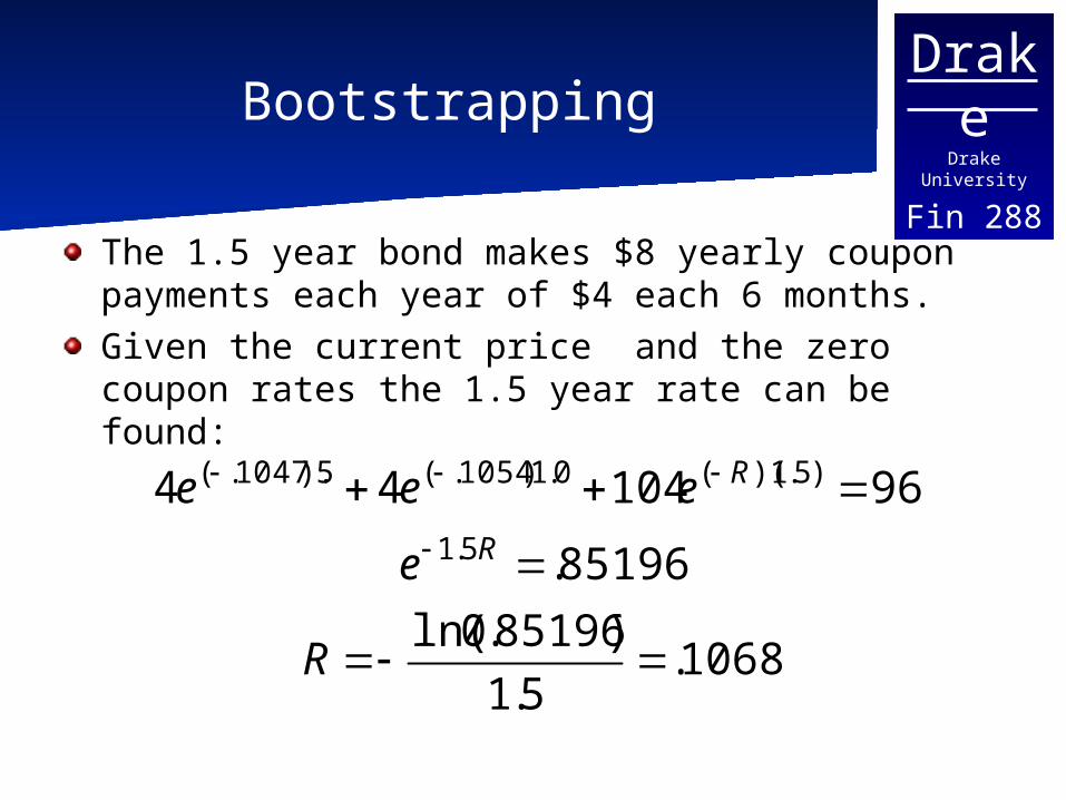
Fin 288Bootstrapping
The 1.5 year bond makes $8 yearly coupon payments each year of $4 each 6 months.Given the current price and the zero coupon rates the 1.5 year rate can be found:
1068.5.1
)85196.0ln(
85196.
96104445.1
)5.1)((0.1)1054.(5).1047.(
R
e
eeeR
R
DrakeDrake University
Fin 288Bootstrapping
You can then solve for the 2 year rate using the 1.5 year rate and the information from the 2 year bond.

DrakeDrake University
Fin 288Forward Rates
Using the theoretical spot curve it is possible to determine a measure of the markets expected future short term rate.Assume you are choosing between buying a 6month zero coupon bond and then reinvesting the money in another 6 month zero coupon bond OR buying a one year zero coupon bond.Today you know the rates on the 6 month and 1 year bonds, but you are uncertain about the future six month rate.
DrakeDrake University
Fin 288Forward Rates
The forward rate is the rate on the future six month bond that would make you indifferent between the two options.
Let z1 = the 6 month zero coupon rate
z22 = the 1 year zero coupon rate (semiannual)f = the rate forward rate from 6 mos to 1 year.
DrakeDrake University
Fin 288Returns
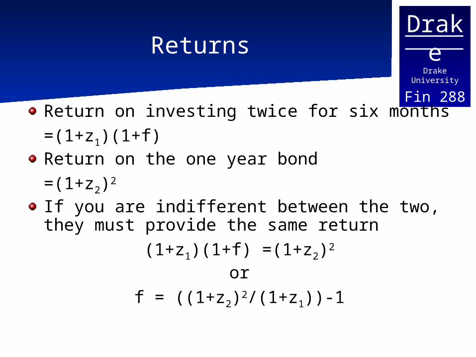
Return on investing twice for six months =(1+z1)(1+f)Return on the one year bond=(1+z2)2
If you are indifferent between the two, they must provide the same return
(1+z1)(1+f) =(1+z2)2
orf = ((1+z2)2/(1+z1))-1
DrakeDrake University
Fin 288Forward Rates
Forward rates do not generally do a good job of actually predicting the future rate, but they do allow the investor to hedgeIf their expectation of the future rate is less than the forward rate they are better off investing for the entire year and lock in the 6 month forward rate over the last 6 months now.
DrakeDrake University
Fin 288
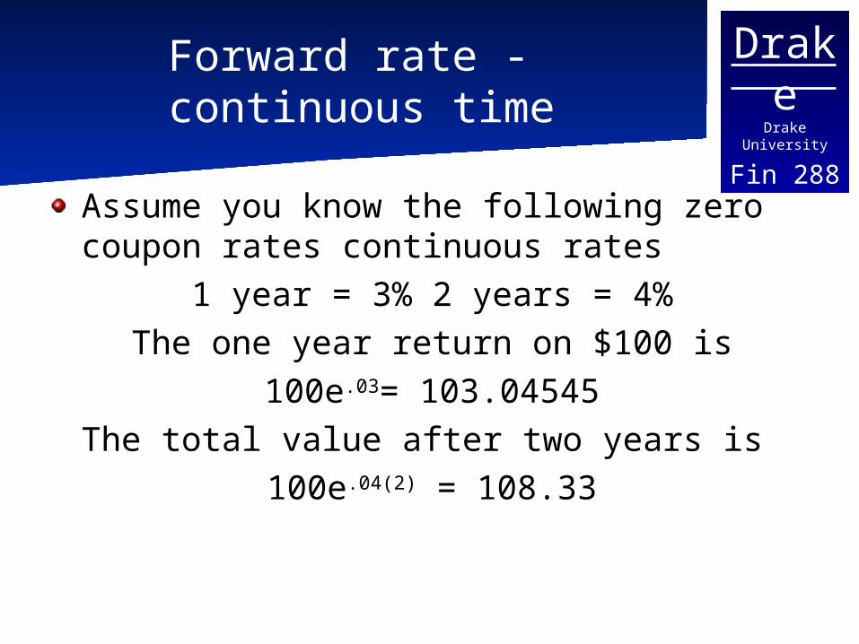
Forward rate - continuous time
Assume you know the following zero coupon rates continuous rates
1 year = 3% 2 years = 4%The one year return on $100 is
100e.03= 103.04545The total value after two years is
100e.04(2) = 108.33
DrakeDrake University
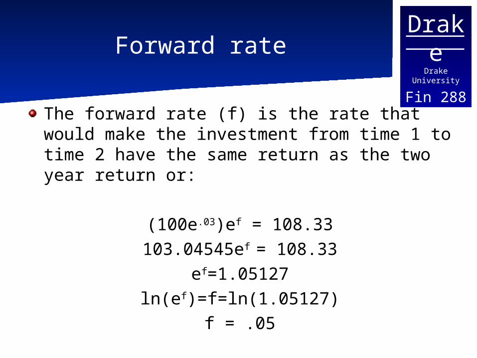
Fin 288Forward rate
The forward rate (f) is the rate that would make the investment from time 1 to time 2 have the same return as the two year return or:
(100e.03)ef = 108.33103.04545ef = 108.33
ef=1.05127ln(ef)=f=ln(1.05127)
f = .05
DrakeDrake University
Fin 288Continuous compounding
Notice that in the previous example the two year rate was the average of the one year rate and the forward rate. This occurs because we are looking at time 1 to time 2 and continuous compounding allows for a nice generalization.
DrakeDrake University
Fin 288
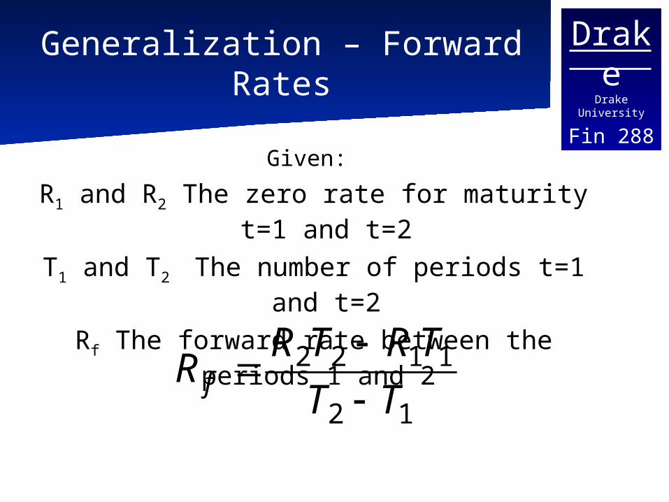
Generalization – Forward Rates
Given:
R1 and R2 The zero rate for maturity t=1 and t=2
T1 and T2 The number of periods t=1 and t=2
Rf The forward rate between the periods 1 and 2
12
1122
TT
TRTRR f
DrakeDrake University
Fin 288Treasury Yield Curve
The most commonly investigated and used term structure is the treasury yield curve. (will want to look at zero rates)Treasuries are used since they are:
Considered free of default, and therefore differ only in maturityThe benchmark used to set base ratesExtremely liquid

0
0.01
0.02
0.03
0.04
0.05
0.06
0.00 5.00 10.00 15.00 20.00
Maturity (Years)
Yie
ld
1/30/2004 3/31/2004 7/30/2004 9/30/2005 12/31/2004 1/31/2005
Yield Curves Over the Last Year
DrakeDrake University
Fin 288
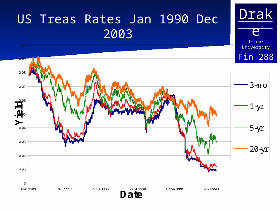
US Treas Rates Jan 1990 Dec 2003
0
0.01
0.02
0.03
0.04
0.05
0.06
0.07
0.08
0.09
0.1
12/8/1989 9/3/1992 5/31/1995 2/24/1998 11/20/2000 8/17/2003
Date
Yie
ld
3-mo
1-yr
5-yr
20-yr

DrakeDrake University
Fin 288
Three Explanations of the Yield Curve
The Expectations TheoriesSegmented Markets TheoryPreferred Habitat Theory

DrakeDrake University
Fin 288Pure Expectations Theory
Long term rates are a representation of the short term interest rates investors expect to receive in the future. In other words the forward rates reflect the future expected rate.Assumes that bonds of different maturities are perfect substitutesIn other words, the expected return from holding a one year bond today and a one year bond next year is the same as buying a two year bond today. (the same process that was used to calculate our forward rates)
DrakeDrake University
Fin 288Pure Expectations
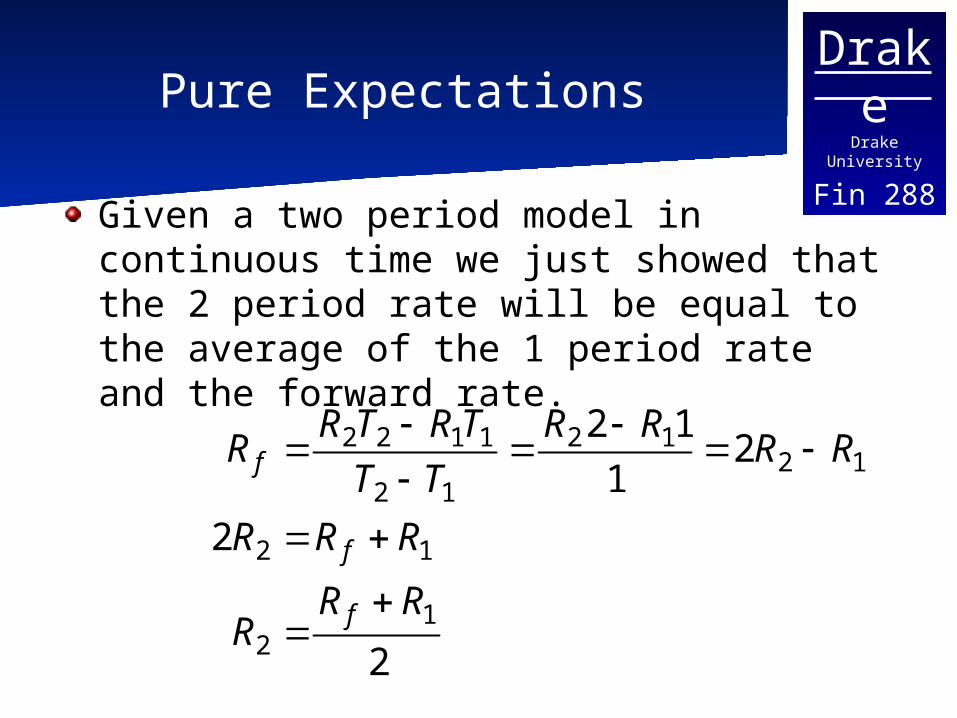
Given a two period model in continuous time we just showed that the 2 period rate will be equal to the average of the 1 period rate and the forward rate.
2
2
21
12
12
12
1212
12
1122
RRR
RRR
RRRR
TT
TRTRR
f
f
f
DrakeDrake University
Fin 288
Expectations Hypothesis R2 = (Rf+R1)/2
When the yield curve is upward sloping (R2>R1) it is expected that short term rates will be increasing (the average future short term rate is above the current short term rate). Likewise when the yield curve is downward sloping the average of the future short term rates is below the current rate. (Fact 2)As short term rates increase the long term rate will also increase and a decrease in short term rates will decrease long term rates. (Fact 1)This however does not explain Fact 3 that the yield curve usually slopes up.
DrakeDrake University
Fin 288
Problems with Pure Expectations
The pure expectations theory ignores the fact that there is reinvestment rate risk and different price risk for the two maturities.Consider an investor considering a 5 year horizon with three alternatives:
buying a bond with a 5 year maturitybuying a bond with a 10 year maturity and holding it 5 yearsbuying a bond with a 20 year maturity and holding it 5 years.
DrakeDrake University
Fin 288Price Risk
The return on the bond with a 5 year maturity is known with certainty the other two are not.
The longer the maturity the greater the price risk
DrakeDrake University
Fin 288Reinvestment rate risk
Now assume the investor is considering a short term investment then reinvesting for the remainder of the five years or investing for five years.
Again the 5 year return is known with certainty, but the others are not.
DrakeDrake University
Fin 288Local expectations
Local expectations theory says that returns of different maturities will be the same over a very short term horizon, for example three months.

DrakeDrake University
Fin 288
Return to maturity expectations hypothesis
This theory claims that the return achieved by buying short term and rolling over to a longer horizon will match the zero coupon return on the longer horizon bond. This eliminates the reinvestment risk.
DrakeDrake University
Fin 288Liquidity Theory
This explanation claims that the since there is a price risk associated with the long term bonds, investor must be offered a premium. Therefore the long term rate reflects both an expectations component and a liquidity premium.This tends to imply that the yield curve will be upward sloping as long as the premium is large enough to outweigh an possible expected decrease.
DrakeDrake University
Fin 288Segmented Markets Theory
Interest Rates for each maturity are determined by the supply and demand for bonds at each maturity.Different maturity bonds are not perfect substitutes for each other.Implies that investors are not willing to accept a premium to switch from their market to a different maturity.Therefore the shape of the yield curve depends upon the asset liability constraints and goals of the market participants.
DrakeDrake University
Fin 288Preferred Habitat Theory
Like the liquidity theory this idea assumes that there is an expectations component and a risk premium.In other words the bonds are substitutes, but savers might have a preference for one maturity over another (they are not perfect substitutes).If there are demand and supply imbalances then investors might be willing to switch to a different maturity.
DrakeDrake University
Fin 288Preferred Habitat Theory
The long term rate should include a premium associated with them. To attract savers who prefer a shorter maturity, the long term bond will need to pay an additional amount or term (liquidity) premium.Thus according to the theory a rise in short term rates still causes a rise in the average of the future short term rates. Therefore the long and short rates move together (Fact 1).
DrakeDrake University
Fin 288Preferred Habitat Theory
The explanation of Fact 2 from the expectations hypothesis still works. In the case of a downward sloping yield curve, the term premium (interest rate risk) must not be large enough to compensate for the currently high short term rates (Current high inflation with an expectation of a decrease in inflation). Since the demand for the short term bonds will increase, the yield on them should fall in the future.
DrakeDrake University
Fin 288Preferred Habitat Theory
Fact three is explained since it will be unusual for the term premium to be so small that the yield curve slopes down.
DrakeDRAKE UNIVERSITY
Fin 288
Price Determination in Forward and Futures
Markets
Fin 288Futures Options and Swaps
DrakeDrake University
Fin 288
Determining the delivery price
The delivery price will be determined by the participants expectations about the future price and their willingness to enter into the contract. (Today’s spot price most likely does not equal the delivery price). What else should be considered?
They should both also consider the time value of money
DrakeDrake University
Fin 288
Theoretical Pricing of Futures Contracts
The theoretical price Is based upon the elimination of arbitrage opportunities.Start with a simple example:
Assume transaction costs are zeroAssume that storage costs are zero
You have a choice today of purchasing or selling a given asset or entering into a contract to buy or sell it in the future.
DrakeDrake University
Fin 288Theoretical Price
Assume you want to own the asset at a given point in time in the future, You can enter into a long futures position or buy the asset today and hold on to it. If you enter into the futures contract you can invest your cash today and earn interest ( r)
DrakeDrake University
Fin 288Basic Relationship
The Forward Price (F) should equal the spot price (S) plus any interest that could be received on an amount of cash equal to the spot price or:
Note: The book uses continuous compounding to illustrate the same result
Tr)S(1F
DrakeDrake University
Fin 288Eliminating Arbitrage
If the forward price is greater than the spot plus interest an arbitrage opportunity exists.
Borrow to buy the underlying asset in the spot market and take a short position in the futures contract. (for now we will use forward and futures price as if they are the same thing)
Tr)S(1F
DrakeDrake University
Fin 288Numerical Example
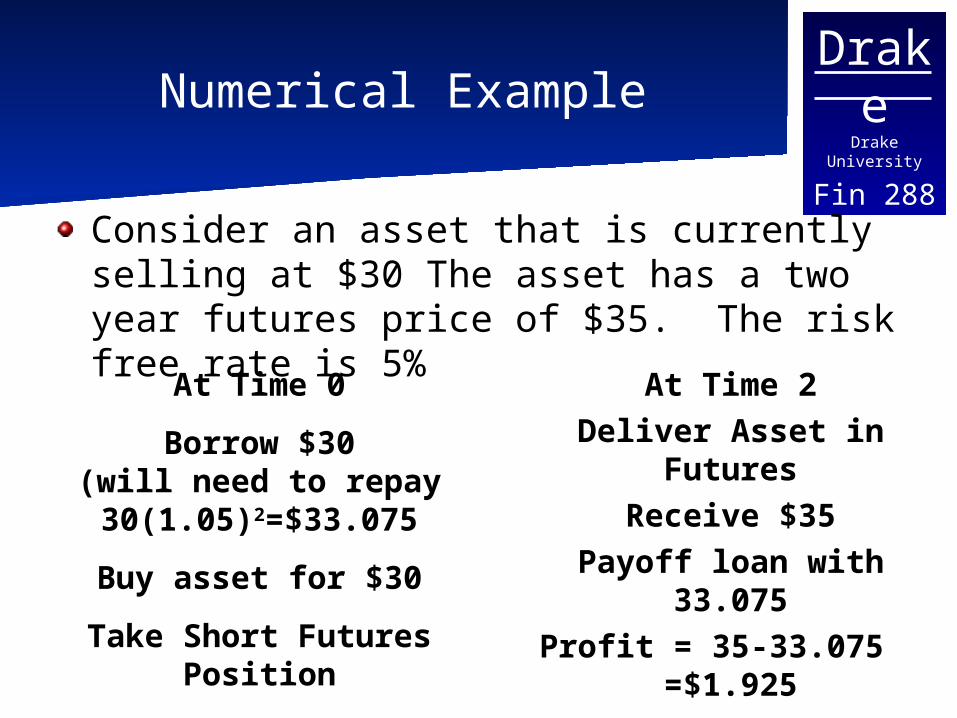
Consider an asset that is currently selling at $30 The asset has a two year futures price of $35. The risk free rate is 5%
At Time 0
Borrow $30(will need to repay 30(1.05)2=$33.075
Buy asset for $30
Take Short Futures Position
At Time 2Deliver Asset in Futures
Receive $35Payoff loan with 33.075
Profit = 35-33.075 =$1.925
DrakeDrake University
Fin 288Example con’t
Increased demand for short contracts, the # of participants willing to sell in two years will be greater than the number willing to buy. Those willing to sell will compete by lowering their price therefore the futures price declines...
DrakeDrake University
Fin 288Eliminating Arbitrage Part 2
What if the futures price is less than the spot price plus interest?Short Sell the underlying asset and take a long position in the futures market
Tr)S(1F
DrakeDrake University
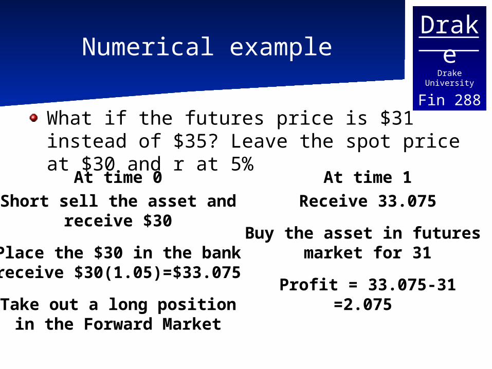
Fin 288Numerical example
What if the futures price is $31 instead of $35? Leave the spot price at $30 and r at 5%
At time 0Short sell the asset and
receive $30
Place the $30 in the bankreceive $30(1.05)=$33.075
Take out a long positionin the Forward Market
At time 1Receive 33.075
Buy the asset in futures market for 31
Profit = 33.075-31=2.075

DrakeDrake University
Fin 288Eliminating Arbitrage
Now there is an excess of participants willing to take a long position but few willing to take a short position. To facilitate trading the futures price will increase. As the price increases it is more attractive to participants willing to take a short position.
DrakeDrake University
Fin 288Eliminating Arbitrage
In both cases the futures price moves toward a point where arbitrage does not exist
When the futures price is 33.075 neither strategy is possible and arbitrage is
eliminated
DrakeDrake University
Fin 288Short Sales
What if it is not possible to short sell the asset?That is not a problem as long as there are enough people that hold the asset that are willing to sell in the futures market.
DrakeDrake University
Fin 288
Paying a known cash income
The above analysis can be extended to the case where the underlying asset pays a known cash income (a treasury bond for example)We are going to assume that the cash payment is due at the same time as the expiration of the forward contract.
DrakeDrake University
Fin 288Cash Income Example
Suppose that you can purchase a treasury bond that makes its coupon payments yearly. If you purchase the bond it will pay a coupon payment of $35 in one year. The bond has a forward price of $950. The risk free rate is 5%.
DrakeDrake University
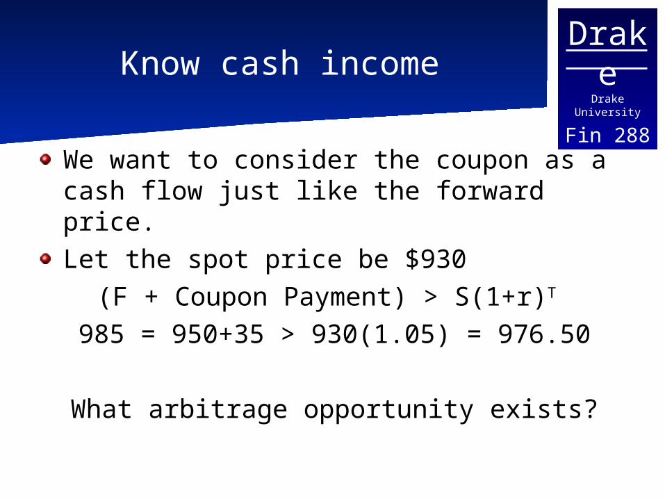
Fin 288Know cash income
We want to consider the coupon as a cash flow just like the forward price.Let the spot price be $930
(F + Coupon Payment) > S(1+r)T 985 = 950+35 > 930(1.05) = 976.50
What arbitrage opportunity exists?
DrakeDrake University
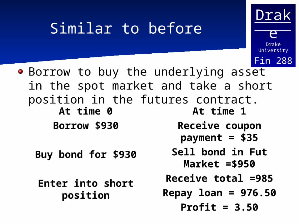
Fin 288Similar to before
Borrow to buy the underlying asset in the spot market and take a short position in the futures contract.
At time 0Borrow $930
Buy bond for $930
Enter into short position
At time 1Receive coupon payment = $35Sell bond in Fut Market =$950
Receive total =985Repay loan = 976.50
Profit = 3.50
DrakeDrake University
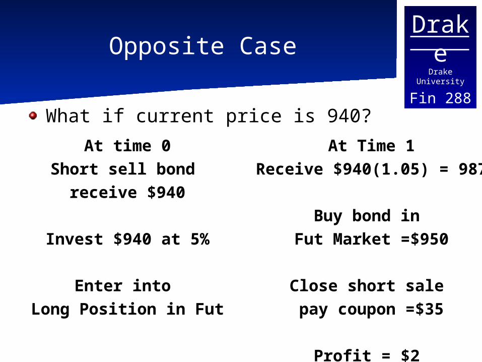
Fin 288Opposite Case
What if current price is 940?
At time 0Short sell bond
receive $940
Invest $940 at 5%
Enter into Long Position in Fut
At Time 1Receive $940(1.05) = 987
Buy bond in Fut Market =$950
Close short sale pay coupon =$35
Profit = $2
DrakeDrake University
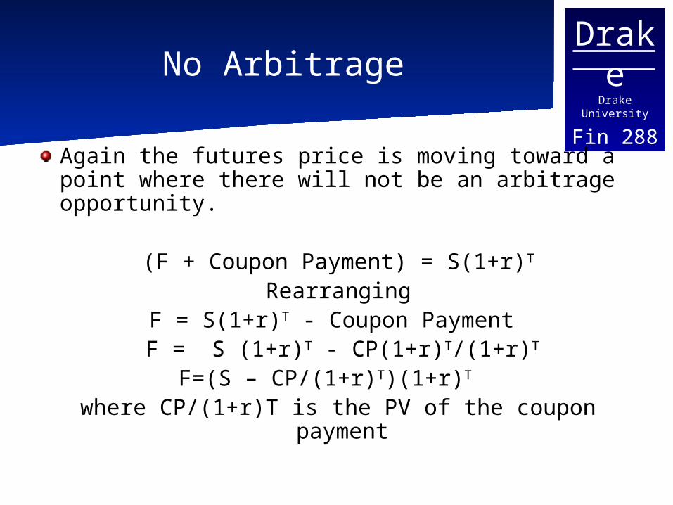
Fin 288No Arbitrage
Again the futures price is moving toward a point where there will not be an arbitrage opportunity.
(F + Coupon Payment) = S(1+r)T
RearrangingF = S(1+r)T - Coupon Payment F = S (1+r)T - CP(1+r)T/(1+r)T
F=(S – CP/(1+r)T)(1+r)T where CP/(1+r)T is the PV of the coupon payment
DrakeDrake University
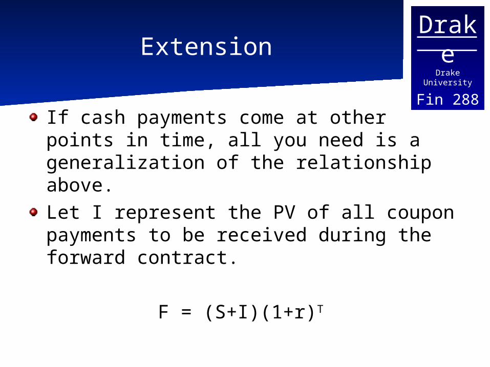
Fin 288Extension
If cash payments come at other points in time, all you need is a generalization of the relationship above.Let I represent the PV of all coupon payments to be received during the forward contract.
F = (S+I)(1+r)T
DrakeDrake University
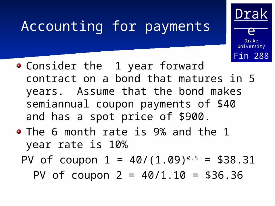
Fin 288Accounting for payments
Consider the 1 year forward contract on a bond that matures in 5 years. Assume that the bond makes semiannual coupon payments of $40 and has a spot price of $900.The 6 month rate is 9% and the 1 year rate is 10%
PV of coupon 1 = 40/(1.09)0.5 = $38.31PV of coupon 2 = 40/1.10 = $36.36
DrakeDrake University
Fin 288
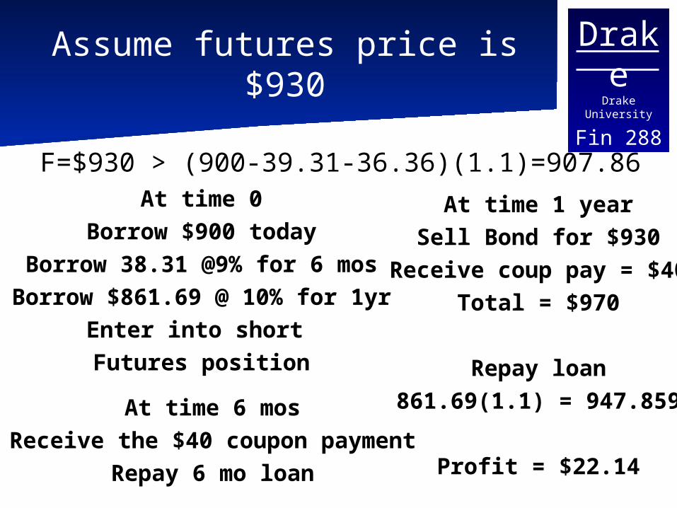
Assume futures price is $930
F=$930 > (900-39.31-36.36)(1.1)=907.86At time 0
Borrow $900 todayBorrow 38.31 @9% for 6 mos
Borrow $861.69 @ 10% for 1yrEnter into short Futures position
At time 6 mosReceive the $40 coupon payment
Repay 6 mo loan
At time 1 yearSell Bond for $930
Receive coup pay = $40Total = $970
Repay loan861.69(1.1) = 947.859
Profit = $22.14
DrakeDrake University
Fin 288Extensions
If the futures price was less than the spot minus the PV of the coupons carried forward an argument similar to the earlier ones could have also been madeA final case is if the income stream pays a known dividend income.
DrakeDrake University
Fin 288Dividend income
Assume that the asset pays a return of q in the future based on the current price of the asset. The equilibrium is then
F = S(1+r)T/(1+q)T
DrakeDrake University
Fin 288Storage Costs?
If the asset has a storage cost (more important for commodities than financial assets), it can be viewed as a negative cash income, the no arbitrage condition would be:
F = (S+U)(1+r)T
Where U represents the present value of all costs.
DrakeDrake University
Fin 288Generalization
Thank of the net amount of any of the possible costs, income received, and interest as the cost of carrying the spot position to the future. It is the cost of holding the spot position instead of the future position.The equilibrium condition is then simply
F = (S+C)(1+rc)T
C is any cash income / costs and rc is net interest expense