Embed Size (px)
Citation preview

DrakeDRAKE UNIVERSITY
Fin 284
DrakeDrake University
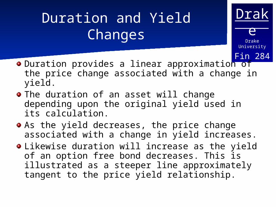
Fin 284Duration and Yield Changes
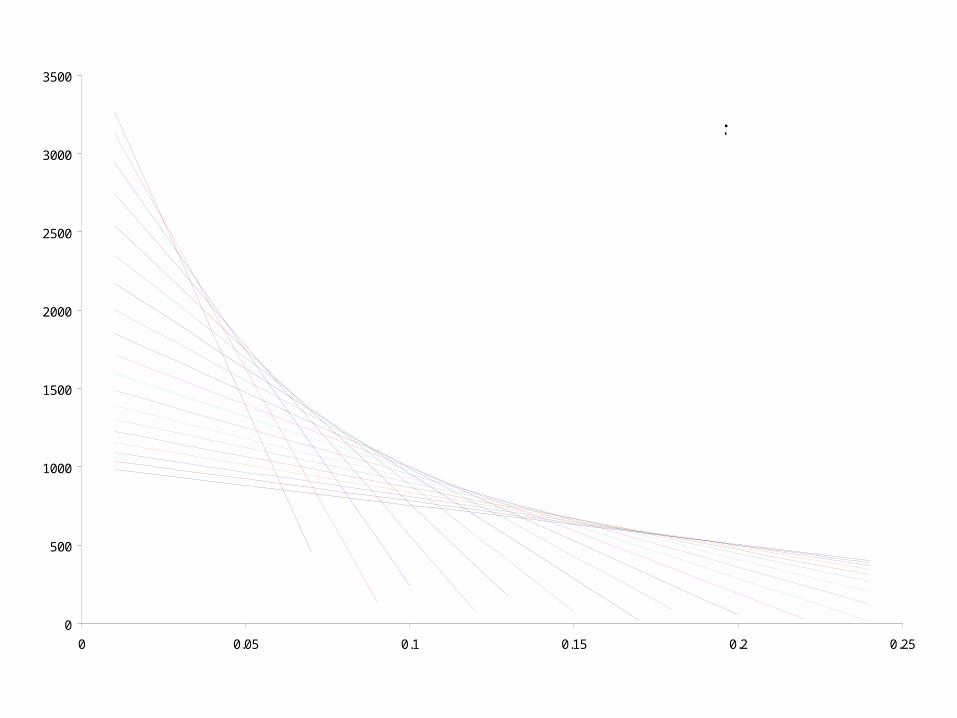
Duration provides a linear approximation of the price change associated with a change in yield. The duration of an asset will change depending upon the original yield used in its calculation. As the yield decreases, the price change associated with a change in yield increases.Likewise duration will increase as the yield of an option free bond decreases. This is illustrated as a steeper line approximately tangent to the price yield relationship.

0
500
1000
1500
2000
2500
3000
3500
0 0.02 0.04 0.06 0.08 0.1 0.12 0.14
Impact of yield on Duration Estimate of Price change

0
500
1000
1500
2000
2500
3000
3500
0 0.05 0.1 0.15 0.2 0.25 0.3
Change in duration outlines the price yield relationship
0
500
1000
1500
2000
2500
3000
3500
0 0.05 0.1 0.15 0.2 0.25
Duration and the Convexity of the Price - Yield Relationship

0
500
1000
1500
2000
2500
3000
3500
0 0.05 0.1 0.15 0.2 0.25
Duration and the Convexity of the Price - Yield Relationship
DrakeDrake University
Fin 284Convexity
The approximation was further from the actual price change the larger the yield change due to the shape of the price yield relationship.It is useful to attempt to measure the error present in the linear duration approximation of the convex price yield relationship.
DrakeDrake University
Fin 284
Approximating the price change
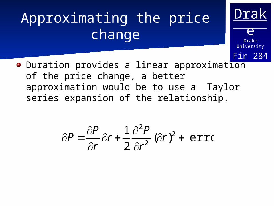
Duration provides a linear approximation of the price change, a better approximation would be to use a Taylor series expansion of the relationship.
error )(2
1 22
2
rr
Pr
r
PP

DrakeDrake University
Fin 284Modified Duration
Previously we showed that modified duration can be estimated by:
Modified duration can be interpreted as the approximate percentage change in price for a 100 basis point change in yield
MODD
rP
P

DrakeDrake University
Fin 284Dollar Duration
The dollar duration represents the dollar change in price for a change in yield, it can be found by multiplying modified duration (which is an approximation for the % change in price) by the original price.
durationdollar D
D
D
MOD
MOD
MOD
Pr
P
PPrP
PrP
P
DrakeDrake University
Fin 284Measuring Convexity
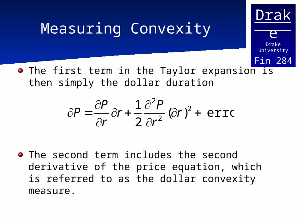
The first term in the Taylor expansion is then simply the dollar duration
The second term includes the second derivative of the price equation, which is referred to as the dollar convexity measure.
error )(2
1 22
2
rr
Pr
r
PP

DrakeDrake University
Fin 284Convexity Mathematics
1n1n432 r)(1
(-n)MV
r)(1
(-n)CP
r)(1
(-3)CP
r)(1
(-2)CP
r)(1
(-1)CP
r
P
nn32 r)(1
MV
r)(1
CP
r)(1
CP
r)(1
CP
r)(1
CPP
2n2n5432
2
r)(1
1)MV(-n)(-(n
r)(1
1)CP(-n)(-(n
r)(1
(-3)(-4)CP
r)(1
(-2)(-3)CP
r)(1
(-1)(-2)CP
r
P
2n2t2
2
r)(1
1)MV(n)(n
r)(1
1)CP(t)(t
r
P

DrakeDrake University
Fin 284Dollar Convexity Measure
The second derivative of the price equation is referred to as the dollar convexity measure
The Convexity Measure and is simply the dollar convexity measure divided by price
2
2
r
P
Pr
P 1
2
12
2
DrakeDrake University
Fin 284
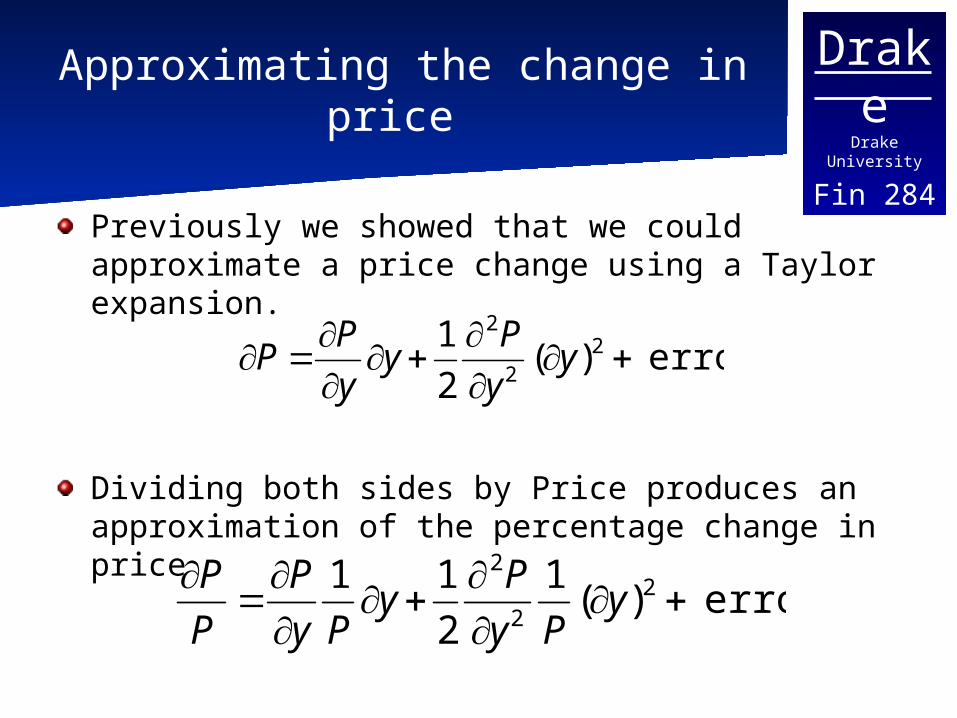
Approximating the change in price
Previously we showed that we could approximate a price change using a Taylor expansion.
Dividing both sides by Price produces an approximation of the percentage change in price
error )(2
1 22
2
yy
Py
y
PP
error )(1
2
11 22
2
yPy
Py
Py
P
P
P

DrakeDrake University
Fin 284
The percentage change in price
Starting with the Taylor expansion divided by price And substituting from our previous results
We can approximate the price change as
error )(1
2
11 22
2
rPr
Pr
Pr
P
P
P
Measure
Convexity12
2
Py
PMODD
1
Pr
P
error )(Measure
Convexity
2
1D 2
MOD
rr
P
P
DrakeDrake University
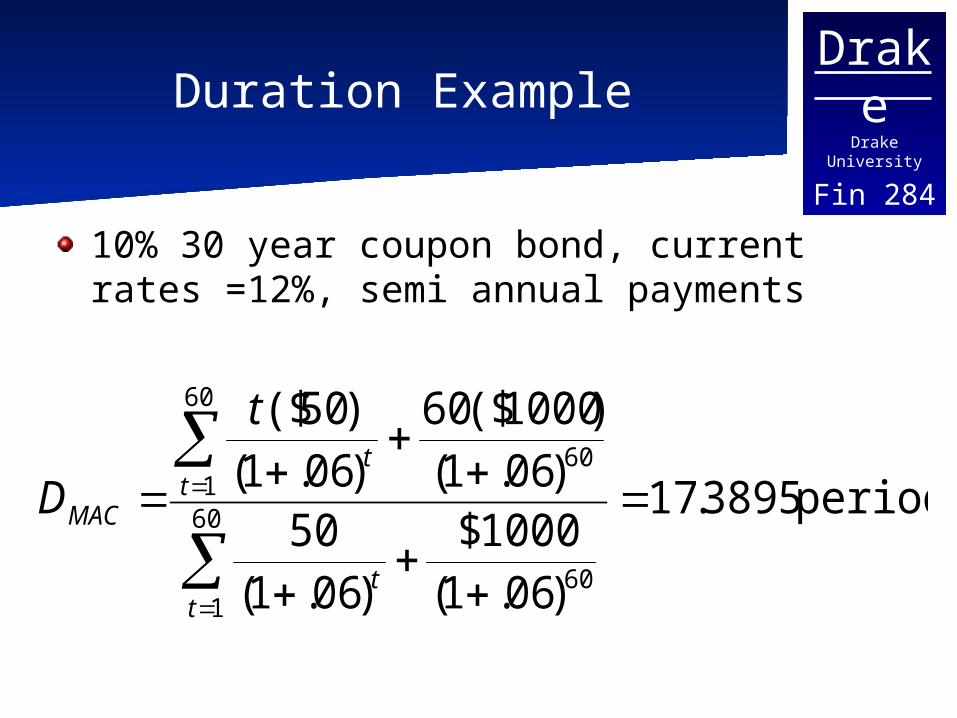
Fin 284Duration Example
10% 30 year coupon bond, current rates =12%, semi annual payments
periods 3895.17
)06.1(1000$
)06.1(50
)06.1()1000($60
)06.1()50($
60
160
60
160
tt
tt
MAC
t
D
DrakeDrake University
Fin 284Example continued
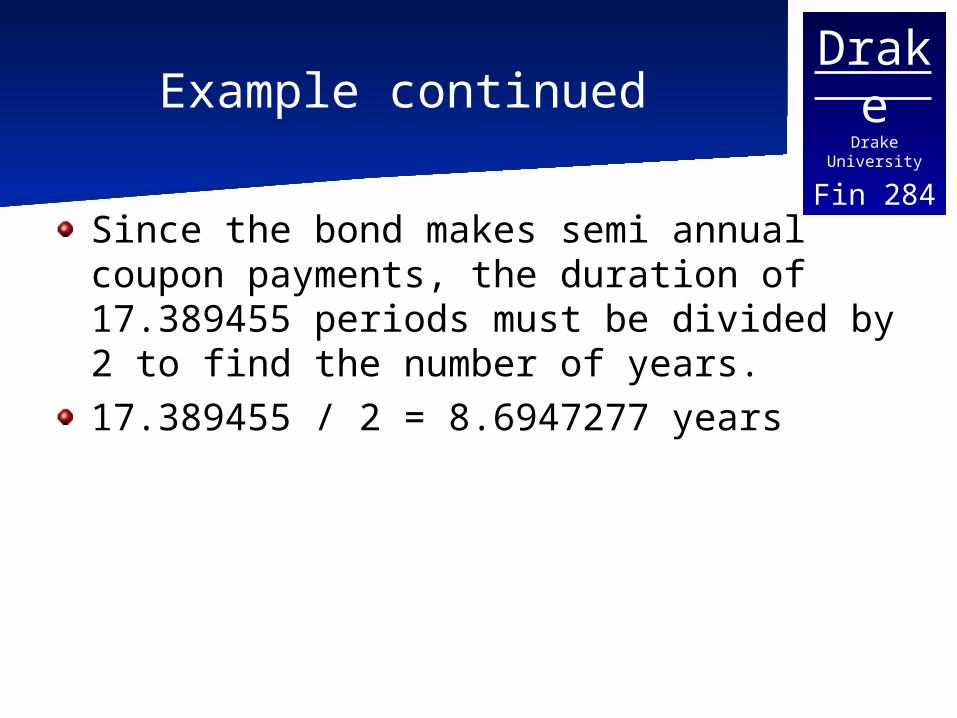
Since the bond makes semi annual coupon payments, the duration of 17.389455 periods must be divided by 2 to find the number of years.17.389455 / 2 = 8.6947277 years
DrakeDrake University
Fin 284
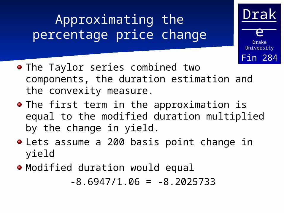
Approximating the percentage price change
The Taylor series combined two components, the duration estimation and the convexity measure.The first term in the approximation is equal to the modified duration multiplied by the change in yield.Lets assume a 200 basis point change in yieldModified duration would equal
-8.6947/1.06 = -8.2025733
DrakeDrake University
Fin 284
Approximating the change in yield continued
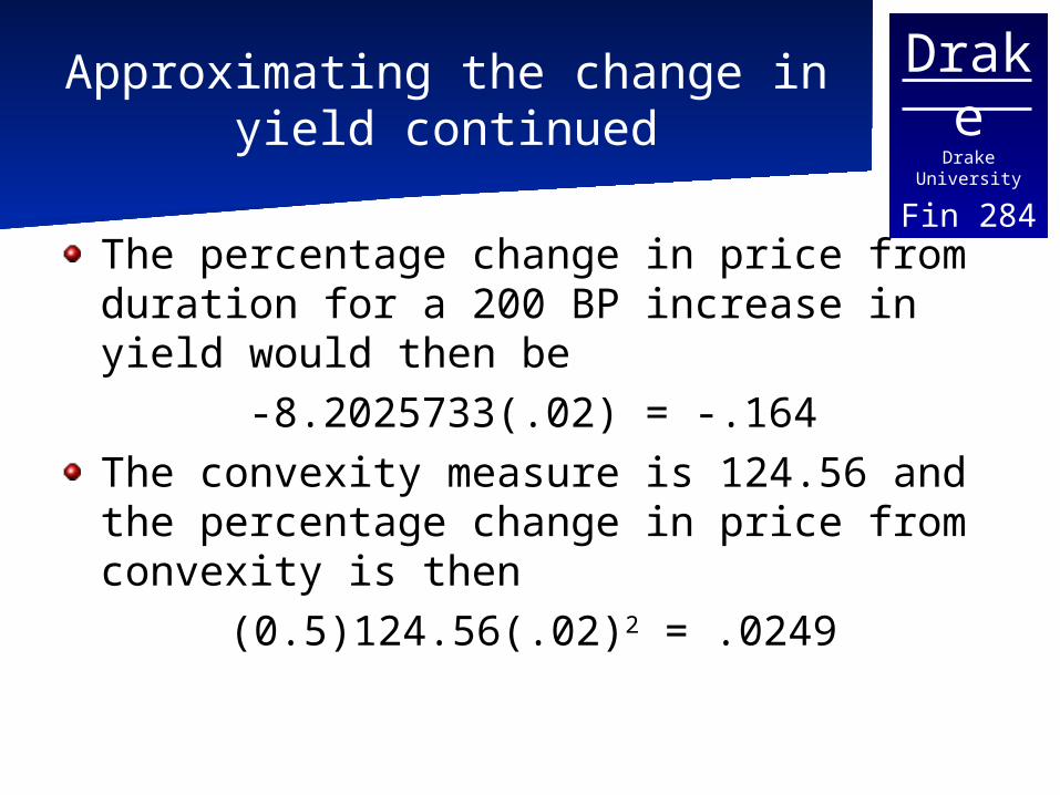
The percentage change in price from duration for a 200 BP increase in yield would then be
-8.2025733(.02) = -.164The convexity measure is 124.56 and the percentage change in price from convexity is then
(0.5)124.56(.02)2 = .0249

DrakeDrake University
Fin 284
Approximating % change in Price continued
The approximate percentage change in price associated with a 200 Bp increase in yield is then the sum of the duration and convexity approximations
Approximate % change = -.164 +.0249 =-.13914
The actual price would be $719.2164 which would be a percentage change of (719.2164-838.3857)/838.3857 = -.14214

DrakeDrake University
Fin 284
Approximating the change in yield continued
The percentage change in price from duration for a 200 BP increase in yield would then be
-8.2025733(-.02) = .164The convexity measure is 124.56 and the percentage change in price from convexity is then
(0.5)124.56(.02)2 = .0249
DrakeDrake University
Fin 284
Approximating % change in Price continued
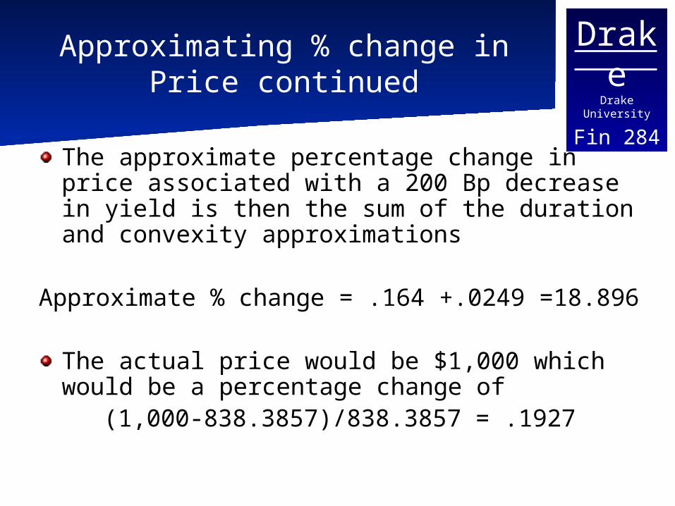
The approximate percentage change in price associated with a 200 Bp decrease in yield is then the sum of the duration and convexity approximations
Approximate % change = .164 +.0249 =18.896
The actual price would be $1,000 which would be a percentage change of
(1,000-838.3857)/838.3857 = .1927

DrakeDrake University
Fin 284Convexity Adjustment
In both cases the approximation using convexity is much closer to the actual price change than the approximation using only duration.
DrakeDrake University
Fin 284Convexity Intuition
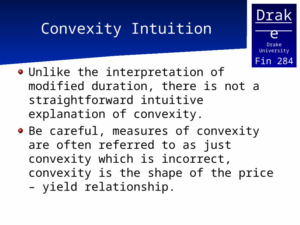
Unlike the interpretation of modified duration, there is not a straightforward intuitive explanation of convexity.Be careful, measures of convexity are often referred to as just convexity which is incorrect, convexity is the shape of the price – yield relationship.

DrakeDrake University
Fin 284Value of Convexity
In comparing two bonds with the same duration, the same yield, and selling a the same price the one that is more convex will have a higher price if yield changes.This implies that the capital loss associated with an increasing yield will be less for the more convex bond and the capital gain associated with a decrease in yield will be greater. Generally the greater convexity, the lower the yield since the price risk is less.
DrakeDrake University
Fin 284
Properties of Convexity on option free bonds
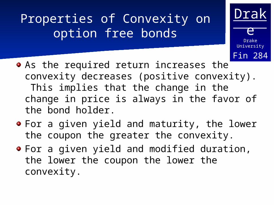
As the required return increases the convexity decreases (positive convexity). This implies that the change in the change in price is always in the favor of the bond holder.For a given yield and maturity, the lower the coupon the greater the convexity.For a given yield and modified duration, the lower the coupon the lower the convexity.

DrakeDrake University
Fin 284Approximating Convexity
The procedure used so far is lengthy and can be approximated similar to the approximation of duration.
DrakeDrake University
Fin 284
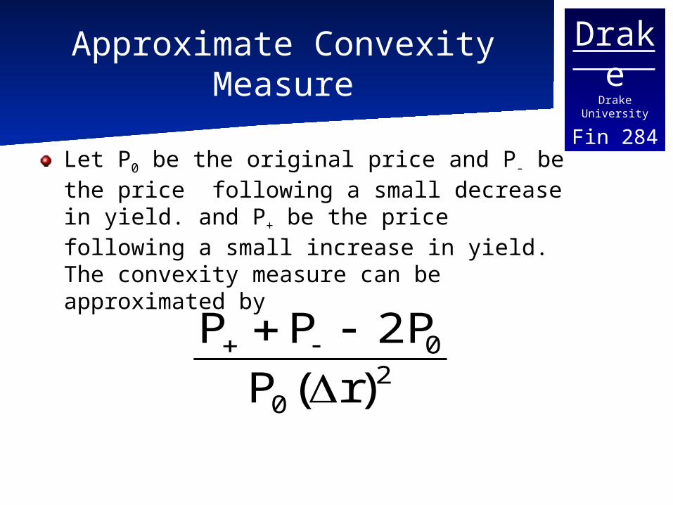
Approximate Convexity Measure
Let P0 be the original price and P- be the price following a small decrease in yield. and P+ be the price following a small increase in yield. The convexity measure can be approximated by
20
0
)r(P
2PPP
DrakeDrake University
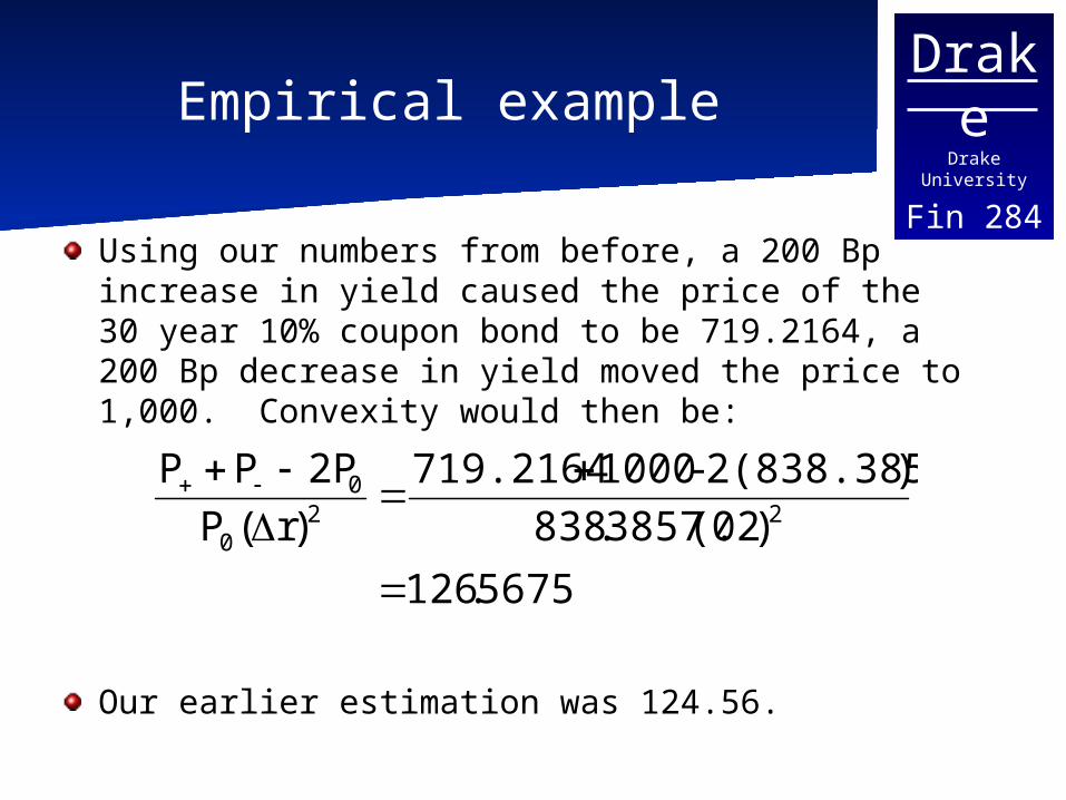
Fin 284Empirical example
Using our numbers from before, a 200 Bp increase in yield caused the price of the 30 year 10% coupon bond to be 719.2164, a 200 Bp decrease in yield moved the price to 1,000. Convexity would then be:
Our earlier estimation was 124.56.
5675.126
)02(.3857.838
)2(838.3857-1000719.2164
)r(P
2PPP22
0
0

DrakeDrake University
Fin 284Convexity and software
The calculation of convexity varies when using software. Often the convexity measure is already divided by 2. In our example before we divided it by 2 when calculating the % price change. Other times it is scaled to account for the par value. The key is knowing how it is calculated when making the adjustment to the duration estimation.
DrakeDrake University
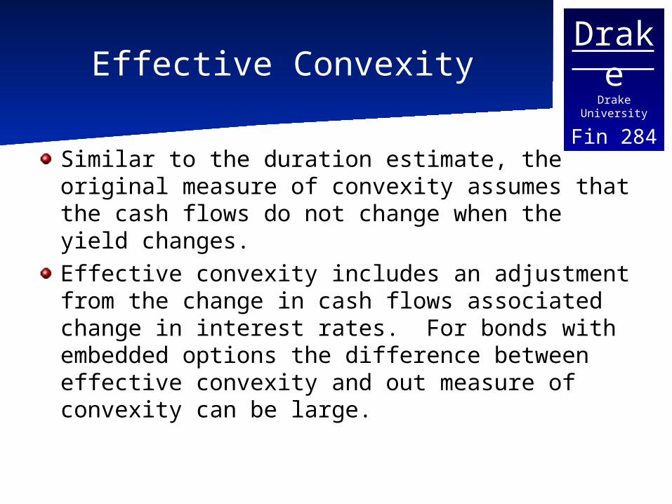
Fin 284Effective Convexity
Similar to the duration estimate, the original measure of convexity assumes that the cash flows do not change when the yield changes. Effective convexity includes an adjustment from the change in cash flows associated change in interest rates. For bonds with embedded options the difference between effective convexity and out measure of convexity can be large.

DrakeDrake University
Fin 284
Bonds with call and put options
So far we have assumed that the bond is option free. If the bond has embedded options it can change the shape of the price-yield relationship.

DrakeDrake University
Fin 284Call Options
With a call option, as yield declines it is more likely that the bond will be called. The value of the bond if called is less than than if it isn’t.As the yield declines the bond may exhibit negative convexity – the increase in price associated with successive decreases in yield will be less (not greater as in the case of positive convexity).

DrakeDrake University
Fin 284Put options
With a put option, as the yield increases the likelihood of the option being exercised increases.Since this adds value to the bond, the price yield relationship will become more convex as yield increases compared to an option free bond with the same characteristics.

DrakeDrake University
Fin 284Interest Rates
So far we have assumed that interest rates behave the same in relation to all bonds. However because of the term structure of interest rates, and other factors impacting the risk premium, the interest rate volatility of bonds differsTo understand how this impacts the bond valuation process and price – yield relationship we need to expand our understanding of interest rates.
DrakeDrake University
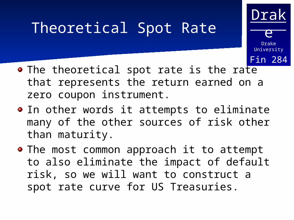
Fin 284Theoretical Spot Rate
The theoretical spot rate is the rate that represents the return earned on a zero coupon instrument. In other words it attempts to eliminate many of the other sources of risk other than maturity.The most common approach it to attempt to also eliminate the impact of default risk, so we will want to construct a spot rate curve for US Treasuries.

DrakeDrake University
Fin 284
Theoretical Spot Rate Curves
Two main issues1. Given a series of Treasury securities, how do
you construct the yield curve?a. Linear Extrapolationb. Bootstrappingc. Other
2. What Treasuries should be used to construct it?a. On the run Treasuriesb. On the run Treasuries and selected off the
run Treasuriesc. All Treasury Coupon Securities and Billsd. Treasury Coupon Strips

DrakeDrake University
Fin 284Observed Yields
For on-the-run treasury securities you can observe the current yield. For the coupon bearing bonds the yield used reflects the yield that would make it trade at par. The resulting on the run curve is the par coupon curve.However, you may have missing maturities for the on the run issues. Then you will need to estimate the missing maturities.
DrakeDrake University
Fin 284Example
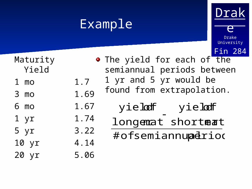
MaturityYield
1 mo 1.73 mo 1.696 mo 1.671 yr 1.745 yr 3.2210 yr 4.1420 yr 5.06
The yield for each of the semiannual periods between 1 yr and 5 yr would be found from extrapolation.
periods semiannual of #
matshorter
of yield
matlonger
of yield
DrakeDrake University
Fin 284
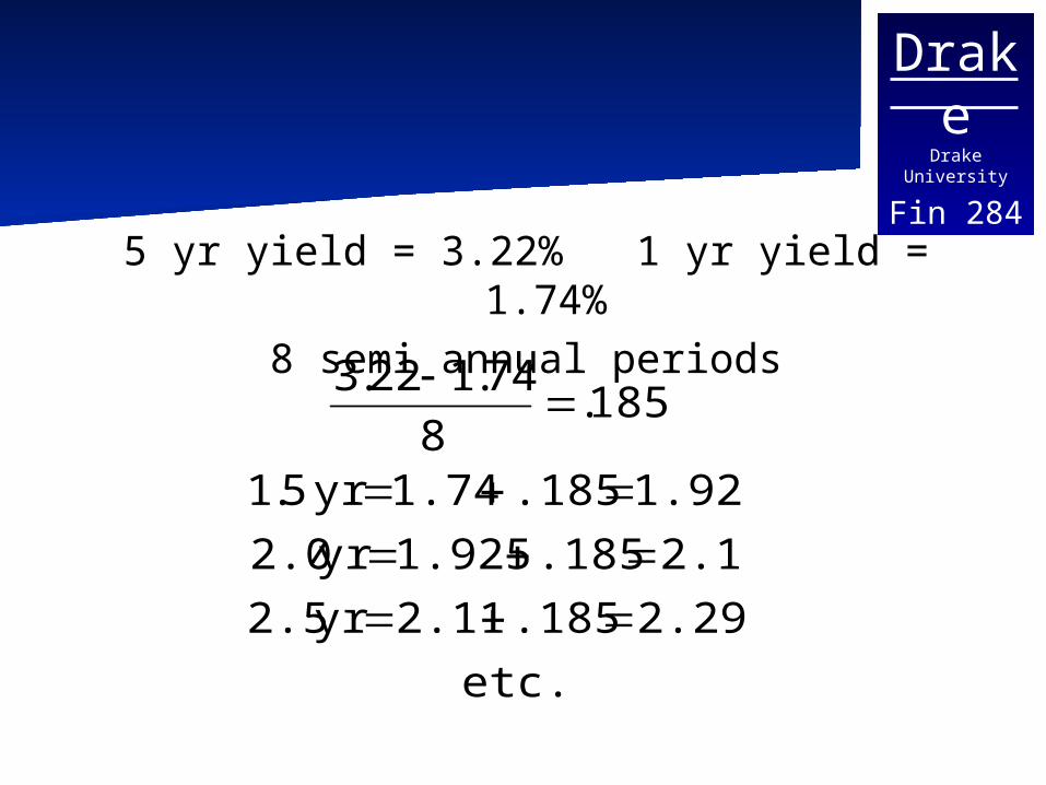
5 yr yield = 3.22% 1 yr yield = 1.74%8 semi annual periods
etc.
2.295.1852.11 yr 2.5
2.11 .1851.925 yr 2.0
1.925.185 1.74 yr 5.1
185.8
74.122.3
DrakeDrake University
Fin 284Bootstrapping
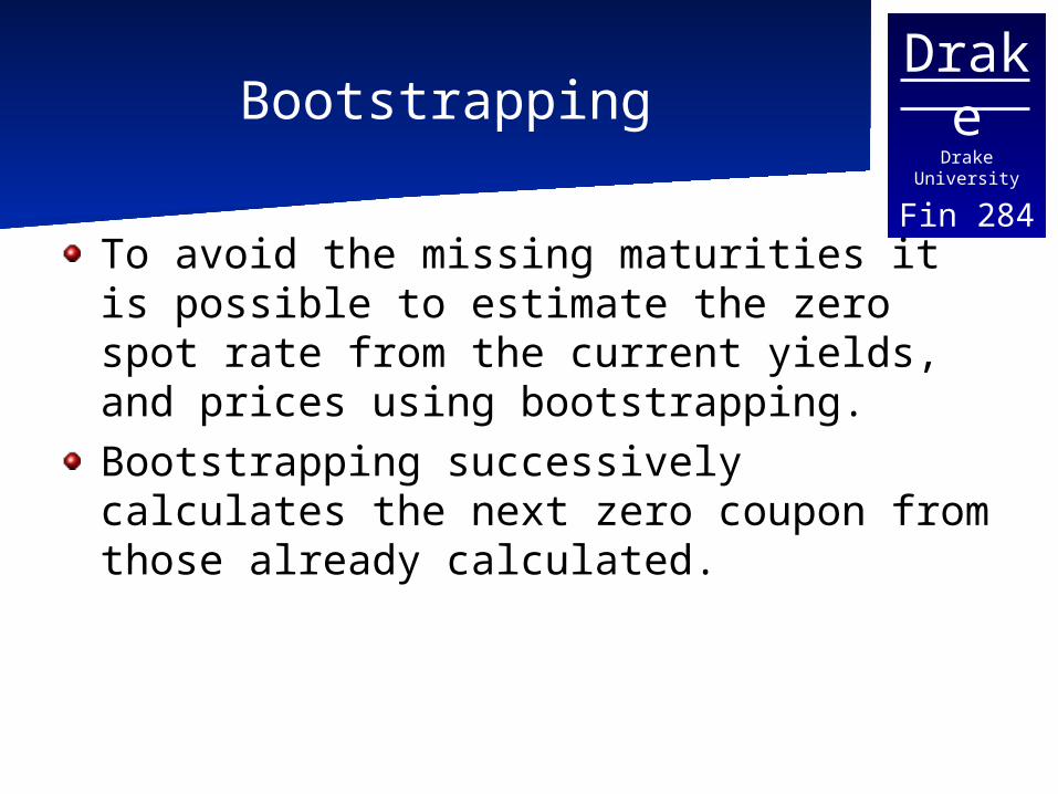
To avoid the missing maturities it is possible to estimate the zero spot rate from the current yields, and prices using bootstrapping. Bootstrapping successively calculates the next zero coupon from those already calculated.
DrakeDrake University
Fin 284
Treasury Bills vs. Notes and Bonds
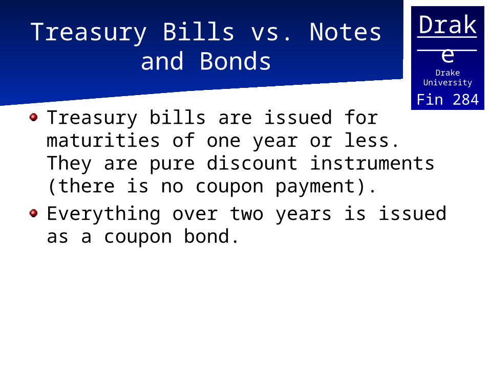
Treasury bills are issued for maturities of one year or less. They are pure discount instruments (there is no coupon payment).Everything over two years is issued as a coupon bond.
DrakeDrake University
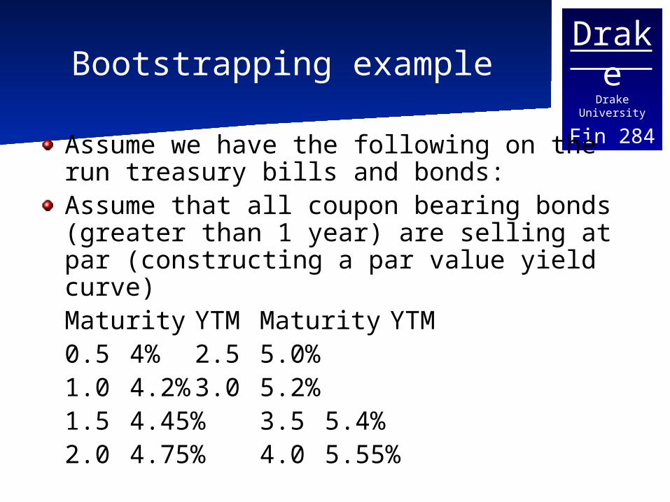
Fin 284Bootstrapping example
Assume we have the following on the run treasury bills and bonds:Assume that all coupon bearing bonds (greater than 1 year) are selling at par (constructing a par value yield curve)Maturity YTM Maturity YTM0.5 4% 2.5 5.0%1.0 4.2% 3.0 5.2%1.5 4.45% 3.5 5.4%2.0 4.75% 4.0 5.55%

DrakeDrake University
Fin 284Bootstrapping continued
Since the 6 month and one year bills are zero coupon instruments we will use them to estimate the zero coupon 1.5 year rate.The 1.5 year note would make a semiannual coupon payment of $100(.0445)/2=2.225Therefore the cash flows from the bond would bet0.5=2.225 t1=2.225 t1.5=102.225
DrakeDrake University
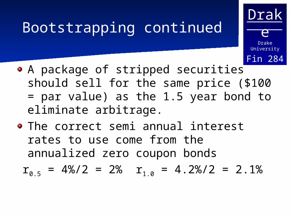
Fin 284Bootstrapping continued
A package of stripped securities should sell for the same price ($100 = par value) as the 1.5 year bond to eliminate arbitrage.The correct semi annual interest rates to use come from the annualized zero coupon bonds
r0.5 = 4%/2 = 2% r1.0 = 4.2%/2 = 2.1%

DrakeDrake University
Fin 284Bootstrapping continued
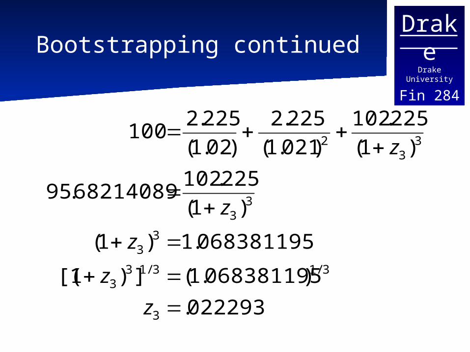
r0.5 = 4%/2 = 2% r1.0 = 4.2%/2 = 2.1%
The price of the package of zero coupons should equal the price of the theoretical
1.5 year zero coupon
3
32 )1(
225.102
)021.1(
225.2
)02.1(
225.2100
z
DrakeDrake University
Fin 284Bootstrapping continued
022293.
)068381195.1(])1[(
068381195.1)1(
)1(
225.10268214089.95
)1(
225.102
)021.1(
225.2
)02.1(
225.2100
3
3/13/133
33
33
33
2
z
z
z
z
z

DrakeDrake University
Fin 284Bootstrapping continued
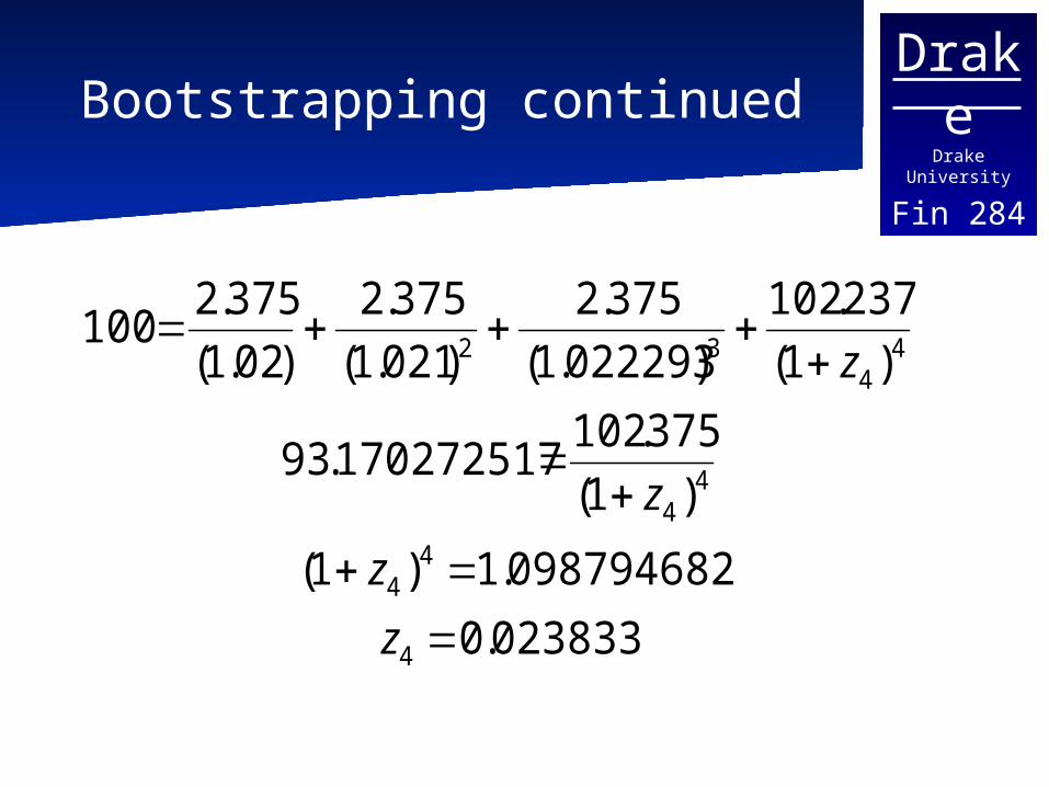
The semi annual rate is therefore 2.2293% and the annual yield would be 4.4586%Similarly the 2 year yield could be found:the coupon is 4.75% implying coupon payments of $2.375 and cash flows of:
t0.5=2.375 t1.0=2.375 t1.5=2.375 t2.0=102.375
44
32 )1(
375.102
)022293.1(
375.2
)021.1(
375.2
)02.1(
375.2100
z
DrakeDrake University
Fin 284Bootstrapping continued
023833.0
098794682.1)1(
)1(
375.102170272517.93
)1(
237.102
)022293.1(
375.2
)021.1(
375.2
)02.1(
375.2100
4
44
44
44
32
z
z
z
z
DrakeDrake University
Fin 284Bootstrapping continued
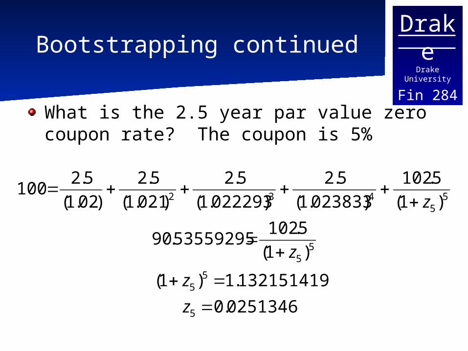
What is the 2.5 year par value zero coupon rate? The coupon is 5%
0251346.0
132151419.1)1(
)1(
5.10253559295.90
)1(
5.102
)023833.1(
5.2
)022293.1(
5.2
)021.1(
5.2
)02.1(
5.2100
5
55
55
55
432
z
z
z
z

DrakeDrake University
Fin 284Adding off the run securities
You can fill in the larger gaps in maturity by adding selected off the run securities especially at the higher end of the maturity range.After extrapolating the missing maturities use the bootstrapping method to calculate the hypothetical zero coupon spot curve.You can also include all securities and use an exponential spline methodology
DrakeDrake University
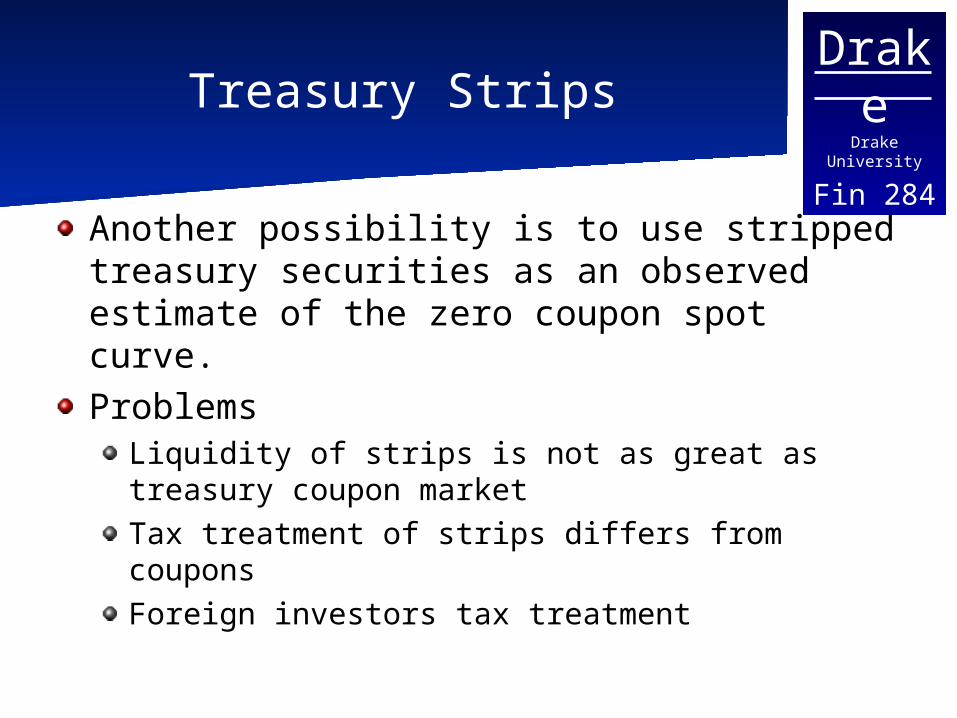
Fin 284Treasury Strips
Another possibility is to use stripped treasury securities as an observed estimate of the zero coupon spot curve.Problems
Liquidity of strips is not as great as treasury coupon marketTax treatment of strips differs from couponsForeign investors tax treatment

DrakeDrake University
Fin 284Using the spot yield curve
Arbitrage should force the price of the treasury to be equal to the total of the cash flows discounted at the zero spot curve.If it does not there is an opportunity for a risk free profit.

DrakeDrake University
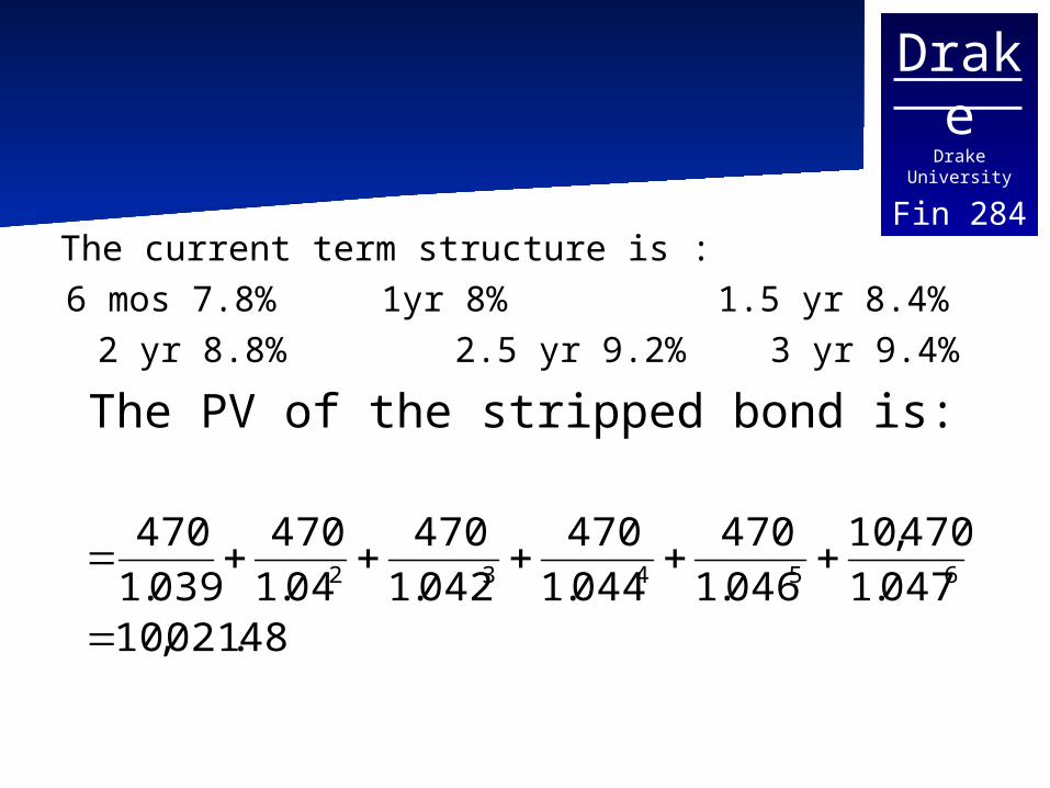
Fin 284Arbitrage Example
Assume you have a 9.4% coupon 3 year treasury notes selling at par. You have purchased a total of $10,000 par value of the note. Current Value$10,000 (since it sells at par)Coupon Payments10,000(.094)/2 = $470 each 6 months
DrakeDrake University
Fin 284
The current term structure is :6 mos 7.8% 1yr 8% 1.5 yr 8.4%
2 yr 8.8% 2.5 yr 9.2% 3 yr 9.4%
The PV of the stripped bond is:
48.021,10047.1
470,10
046.1
470
044.1
470
042.1
470
04.1
470
039.1
47065432

DrakeDrake University
Fin 284Arbitrage continued
You could buy the treasury in the market then sell the stripped coupons for a greater amount.The arbitrage transaction could make $21.48 per 10,000 if exploited.Because of this if the price is not equal to the price of the stripped security using the zero coupon curve, the price should move toward the theoretical price.The theoretical price is termed the Arbitrage free valuation or arbitrage free price.

DrakeDrake University
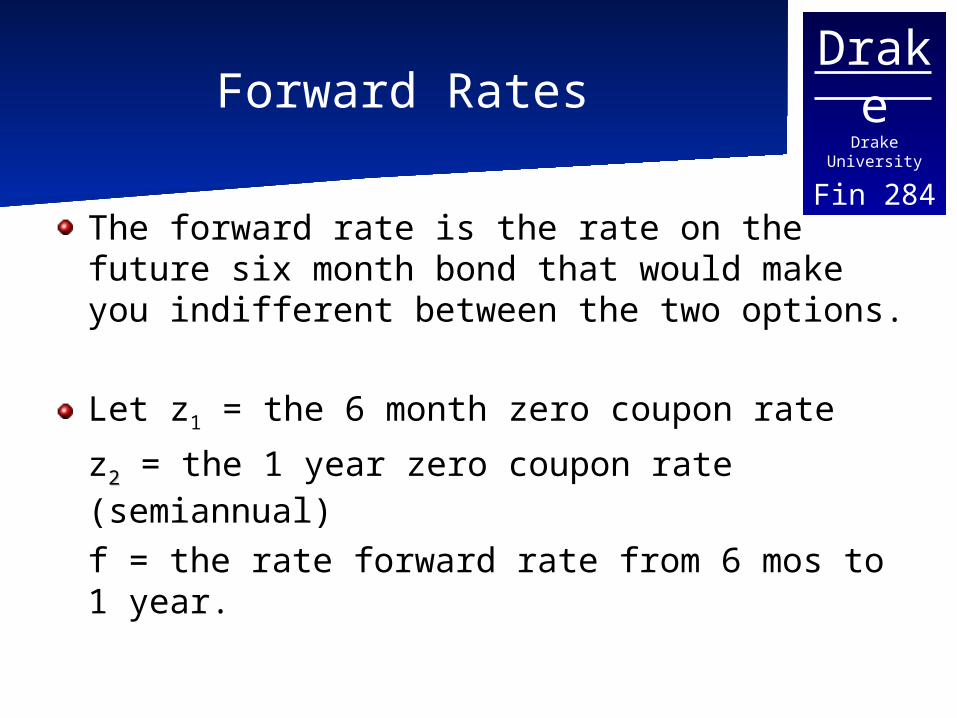
Fin 284Forward Rates
Using the theoretical spot curve it is possible to determine a measure of the markets expected future short term rate.Assume you are choosing between buying a 6month zero coupon bond and then reinvesting the money in another 6 month zero coupon bond OR buying a one year zero coupon bond.Today you know the rates on the 6 month and 1 year bonds, but you are uncertain about the future six month rate.
DrakeDrake University
Fin 284Forward Rates
The forward rate is the rate on the future six month bond that would make you indifferent between the two options.
Let z1 = the 6 month zero coupon rate
z22 = the 1 year zero coupon rate (semiannual)f = the rate forward rate from 6 mos to 1 year.
DrakeDrake University
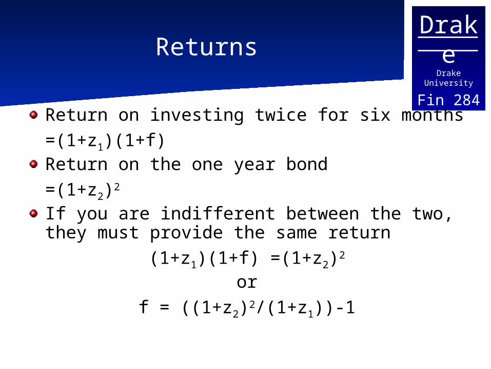
Fin 284Returns
Return on investing twice for six months =(1+z1)(1+f)Return on the one year bond=(1+z2)2
If you are indifferent between the two, they must provide the same return
(1+z1)(1+f) =(1+z2)2
orf = ((1+z2)2/(1+z1))-1
DrakeDrake University
Fin 284Forward Rates
Forward rates do not generally do a good job of actually predicting the future rate, but they do allow the investor to hedgeIf their expectation of the future rate is less than the forward rate they are better off investing for the entire year and lock in the 6 month forward rate over the last 6 months now.