DR2005038 Data Repository Item: Tim Stern pg. 1 Additional information on methods: The original data are contours of subglacial topography. Contours were digitized then rasterized onto a uniform grid using Generic Mapping Tools (GMT) (Smith and Wessel, 1990). Co-ordinates of grid are : x = 0, y = 0: 85 oS, 120 oW; x = 0, y = 300 km: 87.57 oS, 113 oW; x = 1180 km, y = 300 km: 80.17 oS, 147.5 oE; x = 1180 km, y = 0: 79.24 oS, 162 oE The surface fitted to the summits in fig. 3B is done with the surface program within Generic Mapping Tools (GMT) (Smith and Wessel, 1990). Isostatic response function The elastic flexure equation (Watts, 2001) is solved for a 3D elastic sheet using finite difference methods (Stern et al., 1992) . We use the most general partial differential equation describing deformation of a thin elastic plate (Timoshenko & Woinowsky-Krieger , 1959):

∇2(D∇2W ) − (1−ν)(∂2D∂x 2

∂ 2W∂y 2 −

2∂ 2D∂x∂y

∂ 2W∂x∂y

+∂2D∂y 2

∂ 2W∂x 2 ) − Fx

∂ 2W∂x 2 − Fy

∂ 2W∂y 2 − Fxy

∂2W∂x∂y

+ γW = P(x,y)

where : (x,y) = Cartesian coordinates ∇2 = Laplace operator D (x,y) = flexural rigidity = E Te

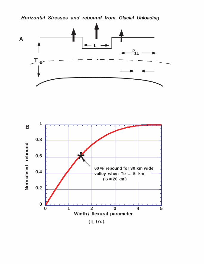
3/ (12(1-ν2)) E = Young’s modulus ν = Poisson’s ratio Te = plate thickness W (x,y) = vertical displacement γ = buoyancy induced stress per unit of vertical displacement ( or restoring force) P(x,y) – vertically acting load Fx = in-plane force in x-direction Fy = in-plane force in y-direction Fxy = in-plane shear force A uniform 5 x 5 km grid is superimposed on the sheet and values of Te, load (in MPa) and restoring force (in g* density contrast(kg/m3 ) is allocated to each grid location. One of the four edges of the elastic plate can be specified as being a free-edge in the sense that no shear stresses can be transmitted over it and the displacements are not required to be zero at the edge. In this study the missing rock due to incision is the load (assumed density of rock = 2700 kg/m3) and the restoring force is then g ∆ρ, where ∆ρ = ρmantle -ρair = ρmantle = 3300 kg/m3, as in isostatic rebound mantle is effectively displacing air. Geological applications of this equation generally make one or more of the simplifying assumptions: that the flexural rigidity D is spatially uniform, that in-plane stresses are negligible and the driving load and deformation vary in one direction only. In this study we make all theses assumptions apart from allowing D (flexural rigidity), restoring force (γ) and load (P) to vary in both x and y directions. Our 3D code was bench-marked for simple shaped loads for which standard analytical solutions exist. These benchmark tests are described in Stern et al. (1992). Relationship between width of valley, flexural parameter and rebound: The wavelength of flexure is controlled by the flexural parameter (α)= 4 D/[(∆ρ)g], where D is the flexural rigidity and ∆ρ is the density contrast between the mantle and infilling material above the plate ( air in the case of rebound) that is displaced by the flexure. If L is the wavelength of erosion, then the dimensionless parameter L/α is what controls the degree of isostatic compensation (Walcott, 1970). For example, with a low Te = 5 km, α = 20 km and for a 30 km wide glacier L/α = 1.5 . At this value rebound is 60 % of the maximum isostatic compensation (Airy compensation). For Te = 20 km, α = 50 km, L/α = 0.5 and only 25 % of Airy compensation is achieved. Fig. 1(supp) shows the calculation for normalized rebound as a function of L/α based on the formula for rebound at the centre of a 2D rectangular mass anomaly(Hetenyi, 1946).

Effect of ice filled valleys The calculations in this study are for rebound due to incision for ice-free conditions. For the free-edge models we calculate the effect of the present ice-fill within the valleys is to reduce the rebound at the

Tim Stern pg. 2 mountain front by a maximum of 200 m. This calculation was done by subtracting a digital representation of the ice sheet elevation (www.ngdc.noaa.gov/) from our DEM for subglacial topography (Fig. 3A), and inserting this into the 3D flexure code described above. Figure Caption: Fig. DR1 a. Cartoon showing upward bending response of lithosphere to the removal of 2D – rectangular mass of width L. P11 represents horizontal stress and is extensional and compressional above and below a neutral plane respectively. Te is the effective elastic thickness. DR1 b. A plot showing the relationship between the dimensionless ratio (L/α) to the normalized rebound (after Walcott, 1970). Hetenyi, M., 1946, Beams on an elastic foundation: Ann Arbour, University of Michigan, 255 p. Smith, W., and Wessel, P., 1990, Gridding with continuous curvature splines in tension: Geophysics, v. 55,

p. 293-305. Stern, T. A., Quinlan, G. M., and Holt, W. E., 1992, Basin formation behind an active subduction zone:

three-dimensional flexural modelling of Wanganui Basin, New Zealand.: Basin Research, v. 4, no. 197 - 214.

Timoshenko, S., and Woinowsky-Krieger, S., 1959, Theory of plates and shells: New York, McGraw-Hill, 462 p.

Walcott, R. I., 1970, An isostatic origin for basement uplifts: Canadian J. of Earth Sciences., v. 7, p. 931 - 937.

Watts, A. B., 2001, Isostasy and flexure of the lithosphere: Cambridge University Press, 458 p.

P

Horizontal Stresses from Glacial Unloading

T e

w L

Horizontal Stresses and rebound from Glacial Unloading

0

0.2

0.4

0.6

0.8

1

0 1 2 3 4 5

No

rmal

ised

re

bo

un

d

Width / flexural parameter

A

B

*60 % rebound for 30 km wide valley when Te = 5 km ( α = 20 km )

L / α )(

11

?

?

extension

Vardar Ocean

Late Triassic

Early-Late Cretaceous

Africa

East Mediterranean ocean

Apulian unit (only western Greece)

Ionian unit & Plattenkalk

Mantle

Gavrovo-Tripolitza unit & Phyllite Quartzite

Pindos unit

Western Vardar ocean

Eastern Vardar ocean (Pindos - Othris ophiolite)

Eastern Vardar ocean (Vardar-Axios zone)

Drama nappe / Getic nappe

Pelagonian unit

Rodope oceanic rift

Moesia nappes

Oceanic lithosphere

Continental lithosphere

Jurassic - Cretaceous turn

Eocene

Neogene

0 km 1000

rollback

?

Middle to Late Jurassic

Pindos & Othris ophiolites

S N

S N

S N

S N

S N

S N